Embed Size (px)
Citation preview
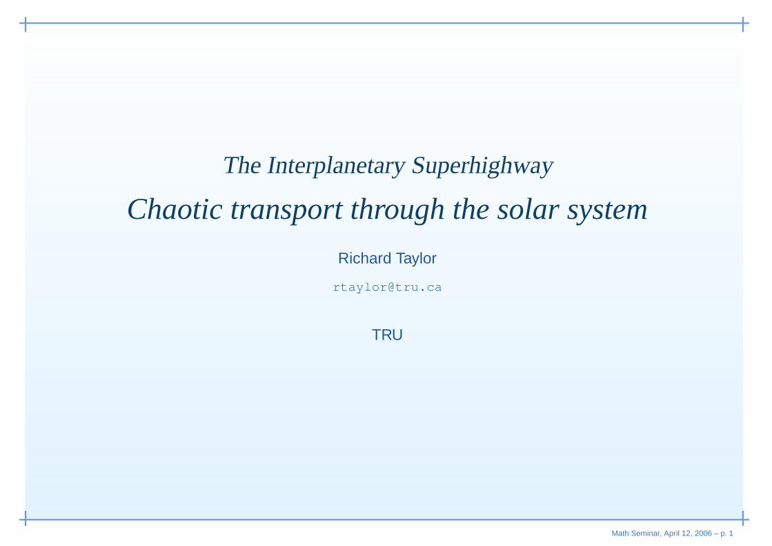
The Interplanetary Superhighway
Chaotic transport through the solar system
Richard Taylor
TRU
Math Seminar, April 12, 2006 – p. 1

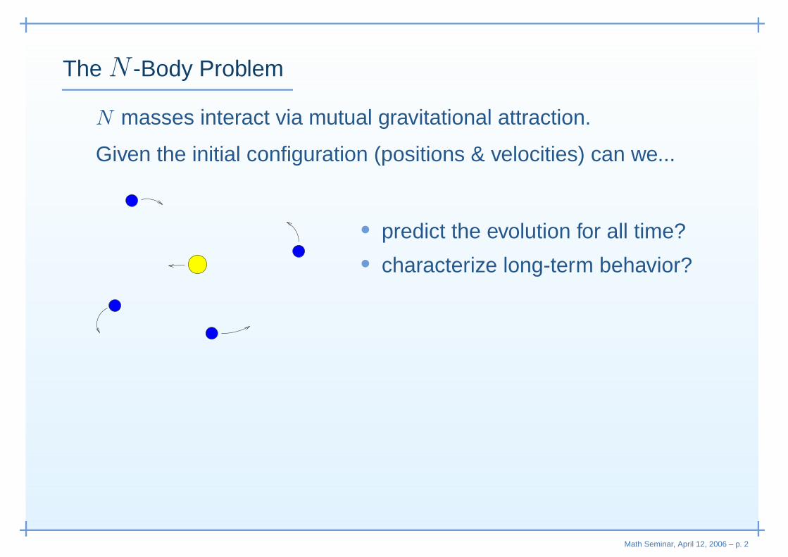
The N -Body Problem
N masses interact via mutual gravitational attraction.
Given the initial configuration (positions & velocities) can we...
• predict the evolution for all time?• characterize long-term behavior?• determine stability?
Math Seminar, April 12, 2006 – p. 2

The N -Body Problem
N masses interact via mutual gravitational attraction.
Given the initial configuration (positions & velocities) can we...
• predict the evolution for all time?
• characterize long-term behavior?• determine stability?
Math Seminar, April 12, 2006 – p. 2
The N -Body Problem
N masses interact via mutual gravitational attraction.
Given the initial configuration (positions & velocities) can we...
• predict the evolution for all time?• characterize long-term behavior?
• determine stability?
Math Seminar, April 12, 2006 – p. 2

The N -Body Problem
N masses interact via mutual gravitational attraction.
Given the initial configuration (positions & velocities) can we...
• predict the evolution for all time?• characterize long-term behavior?• determine stability?
Math Seminar, April 12, 2006 – p. 2

Some History...
• Kepler (∼ 1600) – empirical “laws” of planetary motion
• Newton (∼1700) – solved 2-body problem analytically;planets move on conic sections
• Poincaré (∼ 1900) – 3-body problem is non-integrable• ca. 2000 – basic problems (e.g. stability) are still open
Math Seminar, April 12, 2006 – p. 3

Some History...
• Kepler (∼ 1600) – empirical “laws” of planetary motion• Newton (∼1700) – solved 2-body problem analytically;
planets move on conic sections
• Poincaré (∼ 1900) – 3-body problem is non-integrable• ca. 2000 – basic problems (e.g. stability) are still open
Math Seminar, April 12, 2006 – p. 3

Some History...
• Kepler (∼ 1600) – empirical “laws” of planetary motion• Newton (∼1700) – solved 2-body problem analytically;
planets move on conic sections• Poincaré (∼ 1900) – 3-body problem is non-integrable
• ca. 2000 – basic problems (e.g. stability) are still open
Math Seminar, April 12, 2006 – p. 3

Some History...
• Kepler (∼ 1600) – empirical “laws” of planetary motion• Newton (∼1700) – solved 2-body problem analytically;
planets move on conic sections• Poincaré (∼ 1900) – 3-body problem is non-integrable• ca. 2000 – basic problems (e.g. stability) are still open
Math Seminar, April 12, 2006 – p. 3

So. You want to go to Mars...
How do you get there?
Conventional transport is based on the Hohmann transfer :
• 2-body solutions (conic sections) are pieced together• Most efficient of all possible 2-body trajectories• Still... basically a “brute force” approach• Expensive: $1 million to take 1 lb to the moon• Doesn’t take advantage of N -body dynamics
Math Seminar, April 12, 2006 – p. 4

So. You want to go to Mars...
How do you get there?
Conventional transport is based on the Hohmann transfer :
• 2-body solutions (conic sections) are pieced together
• Most efficient of all possible 2-body trajectories• Still... basically a “brute force” approach• Expensive: $1 million to take 1 lb to the moon• Doesn’t take advantage of N -body dynamics
Math Seminar, April 12, 2006 – p. 4

So. You want to go to Mars...
How do you get there?
Conventional transport is based on the Hohmann transfer :
• 2-body solutions (conic sections) are pieced together• Most efficient of all possible 2-body trajectories
• Still... basically a “brute force” approach• Expensive: $1 million to take 1 lb to the moon• Doesn’t take advantage of N -body dynamics
Math Seminar, April 12, 2006 – p. 4

So. You want to go to Mars...
How do you get there?
Conventional transport is based on the Hohmann transfer :
• 2-body solutions (conic sections) are pieced together• Most efficient of all possible 2-body trajectories• Still... basically a “brute force” approach
• Expensive: $1 million to take 1 lb to the moon• Doesn’t take advantage of N -body dynamics
Math Seminar, April 12, 2006 – p. 4

So. You want to go to Mars...
How do you get there?
Conventional transport is based on the Hohmann transfer :
• 2-body solutions (conic sections) are pieced together• Most efficient of all possible 2-body trajectories• Still... basically a “brute force” approach• Expensive: $1 million to take 1 lb to the moon
• Doesn’t take advantage of N -body dynamics
Math Seminar, April 12, 2006 – p. 4

So. You want to go to Mars...
How do you get there?
Conventional transport is based on the Hohmann transfer :
• 2-body solutions (conic sections) are pieced together• Most efficient of all possible 2-body trajectories• Still... basically a “brute force” approach• Expensive: $1 million to take 1 lb to the moon• Doesn’t take advantage of N -body dynamics
Math Seminar, April 12, 2006 – p. 4

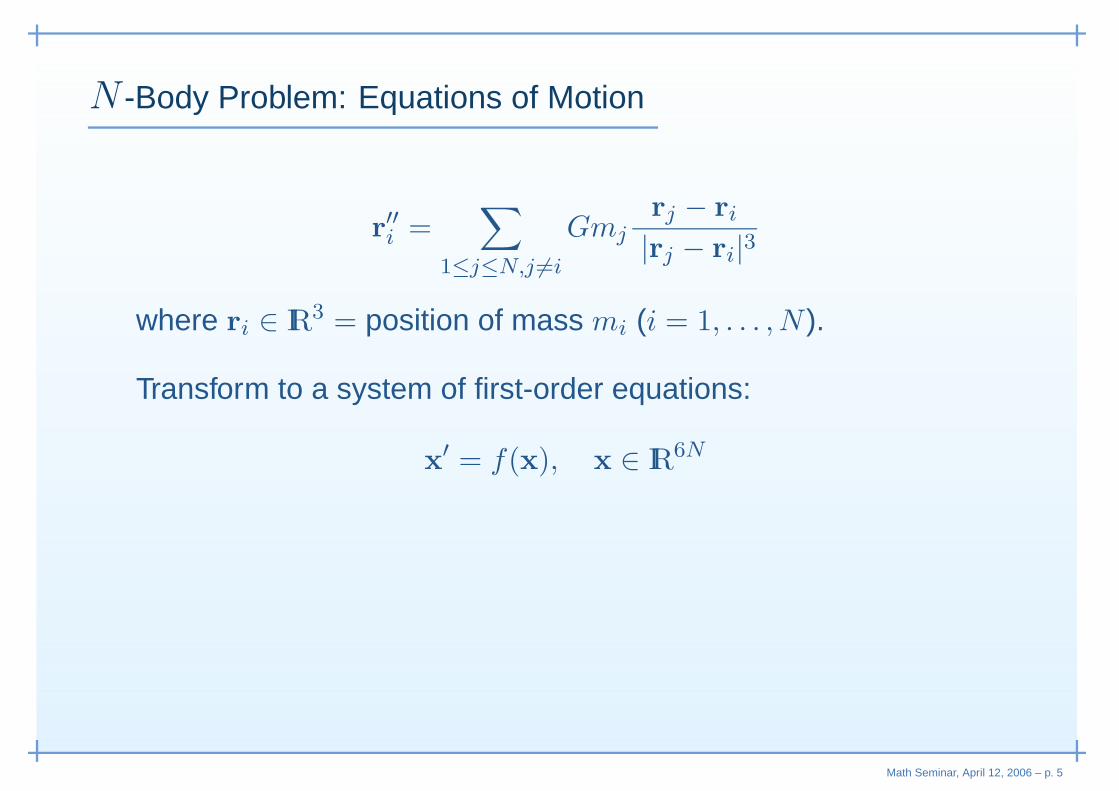
N -Body Problem: Equations of Motion
r′′i =
∑
1≤j≤N,j 6=i
Gmj
rj − ri
|rj − ri|3
where ri ∈ IR3 = position of mass mi (i = 1, . . . , N ).
Transform to a system of first-order equations:
x′ = f(x), x ∈ IR6N
Phase space is 6N -dimensional: 3 position + 3 velocitycoordinates for each of N objects.
Lots of dimensions. Lots of parameters. hrrmmm....
Math Seminar, April 12, 2006 – p. 5

Restricted 3-Body Problem
Planar Circular Restricted 3-Body Problem = PCR3BP
Simplifying assumptions:• all objects move in a single plane
• one object (•) has negligible mass• the other two have circular orbits
<animation>
Math Seminar, April 12, 2006 – p. 6

Restricted 3-Body Problem
Planar Circular Restricted 3-Body Problem = PCR3BP
Simplifying assumptions:• all objects move in a single plane• one object (•) has negligible mass
• the other two have circular orbits
<animation>
Math Seminar, April 12, 2006 – p. 6

Restricted 3-Body Problem
Planar Circular Restricted 3-Body Problem = PCR3BP
Simplifying assumptions:• all objects move in a single plane• one object (•) has negligible mass• the other two have circular orbits
<animation>
Math Seminar, April 12, 2006 – p. 6

Restricted 3-Body Problem
Planar Circular Restricted 3-Body Problem = PCR3BP
Simplifying assumptions:• all objects move in a single plane• one object (•) has negligible mass• the other two have circular orbits
<animation>
Math Seminar, April 12, 2006 – p. 6

PCR3BP: Rotating Coordinate System
• coord. system rotates with circular orbit (ω = 1)
• masses µ, 1 − µ normalized so total mass = 1• origin is at common center of mass
x−µ 1−µ
y
<animation>
Math Seminar, April 12, 2006 – p. 7

PCR3BP: Rotating Coordinate System
• coord. system rotates with circular orbit (ω = 1)• masses µ, 1 − µ normalized so total mass = 1
• origin is at common center of mass
x−µ 1−µ
y
<animation>
Math Seminar, April 12, 2006 – p. 7

PCR3BP: Rotating Coordinate System
• coord. system rotates with circular orbit (ω = 1)• masses µ, 1 − µ normalized so total mass = 1• origin is at common center of mass
x−µ 1−µ
y
<animation>
Math Seminar, April 12, 2006 – p. 7

PCR3BP: Rotating Coordinate System
• coord. system rotates with circular orbit (ω = 1)• masses µ, 1 − µ normalized so total mass = 1• origin is at common center of mass
x−µ 1−µ
y
<animation>
Math Seminar, April 12, 2006 – p. 7

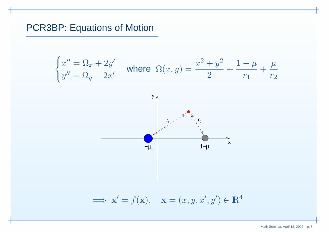
PCR3BP: Equations of Motion
x′′ = Ωx + 2y′
y′′ = Ωy − 2x′where Ω(x, y) =
x2 + y2
2+
1 − µ
r1
+µ
r2
x−µ 1−µ
y
r1 r2
=⇒ x′ = f(x), x = (x, y, x′, y′) ∈ IR4
Math Seminar, April 12, 2006 – p. 8
PCR3BP: Equations of Motion
x′′ = Ωx + 2y′
y′′ = Ωy − 2x′where Ω(x, y) =
x2 + y2
2+
1 − µ
r1
+µ
r2
x−µ 1−µ
y
r1 r2
=⇒ x′ = f(x), x = (x, y, x′, y′) ∈ IR4
Math Seminar, April 12, 2006 – p. 8
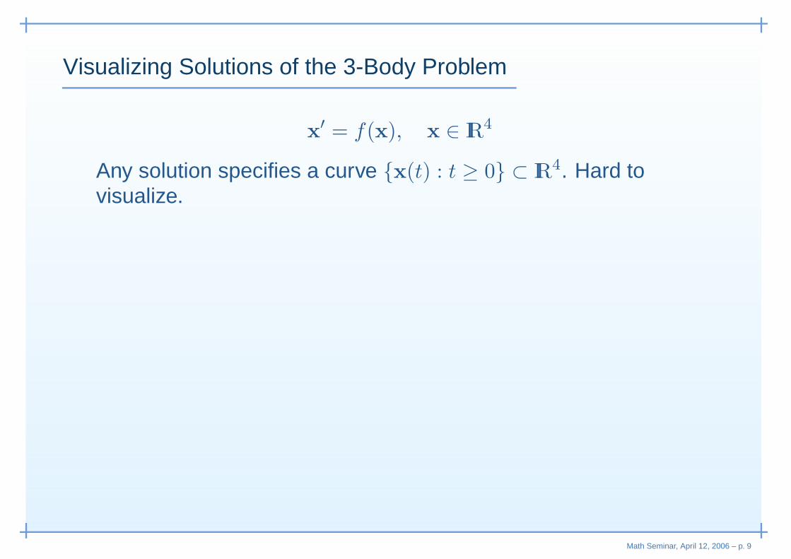
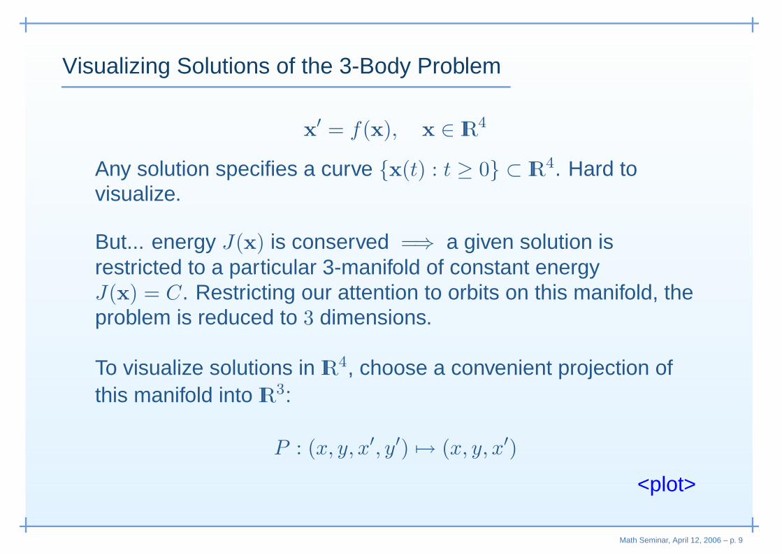
Visualizing Solutions of the 3-Body Problem
x′ = f(x), x ∈ IR4
Any solution specifies a curve x(t) : t ≥ 0 ⊂ IR4. Hard tovisualize.
But... energy J(x) is conserved =⇒ a given solution isrestricted to a particular 3-manifold of constant energyJ(x) = C. Restricting our attention to orbits on this manifold, theproblem is reduced to 3 dimensions.
To visualize solutions in IR4, choose a convenient projection ofthis manifold into IR3:
P : (x, y, x′, y′) 7→ (x, y, x′)
<plot>
Math Seminar, April 12, 2006 – p. 9

Special Case µ = 0
Back to the 2-body problem. Kepler orbit gives a precessingellipse with two rotational frequencies.
x1−1
ω1
2y ω = 1
<animation>
Math Seminar, April 12, 2006 – p. 10

Invariant Tori
In physical space the orbit is a pre-cessing ellipse. The orbit is com-pletely parametrized by two angles. x
1−1
ω1
2y ω = 1
In the phase space IR4, these angles parametrize a curve x(t)
that lies on a torus T 2 ⊂ IR4.
Different initial conditions give a curve x(t) on a different torus.In this way we get a family of nested invariant tori that foliate the3-manifold of constant energy.
<plot><simulation>
Math Seminar, April 12, 2006 – p. 11
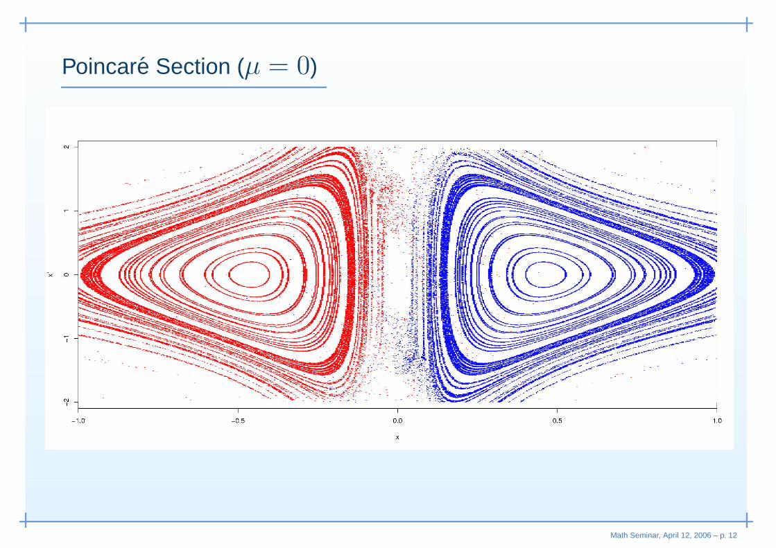
Poincare Section (µ = 0)
Math Seminar, April 12, 2006 – p. 12

Resonance
If ω1
ω2
is irrational then the torus iscovered with a dense orbit (quasi-periodicity ). –1
–0.50
0.51
–1
–0.5
0
0.5
1
–0.4
0
0.4
If ω1
ω2
= mn
is a rational number theorbit is periodic: the spacecraft com-pletes m revolutions just as the planetcompletes n revolutions (resonance).
–1–0.5
00.5
1
–1
–0.5
0
0.5
1
–0.4
0
0.4
Math Seminar, April 12, 2006 – p. 13

Perturbed Case 0 < µ ¿ 1
Theorem (Kolmogorov-Arnold-Moser). For all sufficiently small µ theperturbed system x
′ = f(x) has a set of invariant tori, each of which iscovered with a dense orbit. This set has positive Lebesgue measure.
Only the invariant tori sufficiently far from resonance arepreserved.
Math Seminar, April 12, 2006 – p. 14

Orbits Near Resonance
We know orbits far from resonance are stuck on invariant tori.What about the orbits near resonance?
<animation>
Math Seminar, April 12, 2006 – p. 15

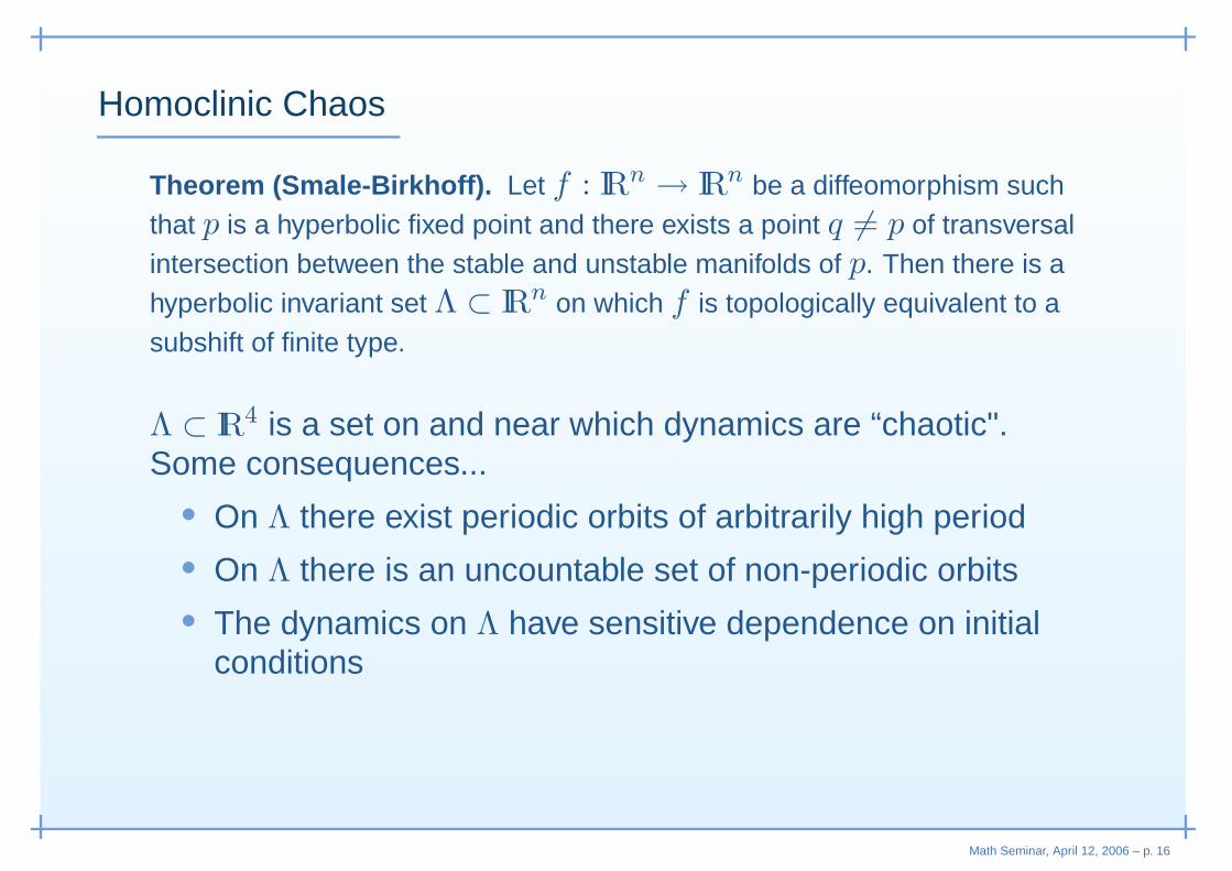
Homoclinic Chaos
Theorem (Smale-Birkhoff). Let f : IRn → IRn be a diffeomorphism suchthat p is a hyperbolic fixed point and there exists a point q 6= p of transversalintersection between the stable and unstable manifolds of p. Then there is ahyperbolic invariant set Λ ⊂ IRn on which f is topologically equivalent to asubshift of finite type.
Λ ⊂ IR4 is a set on and near which dynamics are “chaotic".Some consequences...
• On Λ there exist periodic orbits of arbitrarily high period
• On Λ there is an uncountable set of non-periodic orbits• The dynamics on Λ have sensitive dependence on initial
conditions• Λ is a Cantor set (uncountable, measure-zero) — a fractal
Math Seminar, April 12, 2006 – p. 16

Homoclinic Chaos
Theorem (Smale-Birkhoff). Let f : IRn → IRn be a diffeomorphism suchthat p is a hyperbolic fixed point and there exists a point q 6= p of transversalintersection between the stable and unstable manifolds of p. Then there is ahyperbolic invariant set Λ ⊂ IRn on which f is topologically equivalent to asubshift of finite type.
Λ ⊂ IR4 is a set on and near which dynamics are “chaotic".Some consequences...
• On Λ there exist periodic orbits of arbitrarily high period• On Λ there is an uncountable set of non-periodic orbits
• The dynamics on Λ have sensitive dependence on initialconditions
• Λ is a Cantor set (uncountable, measure-zero) — a fractal
Math Seminar, April 12, 2006 – p. 16
Homoclinic Chaos
Theorem (Smale-Birkhoff). Let f : IRn → IRn be a diffeomorphism suchthat p is a hyperbolic fixed point and there exists a point q 6= p of transversalintersection between the stable and unstable manifolds of p. Then there is ahyperbolic invariant set Λ ⊂ IRn on which f is topologically equivalent to asubshift of finite type.
Λ ⊂ IR4 is a set on and near which dynamics are “chaotic".Some consequences...
• On Λ there exist periodic orbits of arbitrarily high period• On Λ there is an uncountable set of non-periodic orbits• The dynamics on Λ have sensitive dependence on initial
conditions
• Λ is a Cantor set (uncountable, measure-zero) — a fractal
Math Seminar, April 12, 2006 – p. 16

Homoclinic Chaos
Theorem (Smale-Birkhoff). Let f : IRn → IRn be a diffeomorphism suchthat p is a hyperbolic fixed point and there exists a point q 6= p of transversalintersection between the stable and unstable manifolds of p. Then there is ahyperbolic invariant set Λ ⊂ IRn on which f is topologically equivalent to asubshift of finite type.
Λ ⊂ IR4 is a set on and near which dynamics are “chaotic".Some consequences...
• On Λ there exist periodic orbits of arbitrarily high period• On Λ there is an uncountable set of non-periodic orbits• The dynamics on Λ have sensitive dependence on initial
conditions• Λ is a Cantor set (uncountable, measure-zero) — a fractal
Math Seminar, April 12, 2006 – p. 16

Low-Energy Escape from Earth
Contour Plots of Potential Energy Ω(x, y) = x2+y2
2+ 1−µ
r1
+ µr2
= “forbidden region”
−1.5 −1.0 −0.5 0.0 0.5 1.0 1.5
−1.
0−
0.5
0.0
0.5
1.0
Insufficient energy for escape
x
y
−1.5 −1.0 −0.5 0.0 0.5 1.0 1.5
−1.
0−
0.5
0.0
0.5
1.0
Sufficient energy for escape
x
y
Math Seminar, April 12, 2006 – p. 17

Chaos and Low-Energy Escape from Earth
So... to escape Earth with near minimal energy, you must passthrough the “bottleneck" region, and hence exit on a chaotictrajectory.
−1.5 −1.0 −0.5 0.0 0.5 1.0 1.5
−1.
0−
0.5
0.0
0.5
1.0
Sufficient energy for escape
x
y
<animation>Math Seminar, April 12, 2006 – p. 18

Transport on low-energy trajectories
• Half the energy requirements of a Hohmann transfer
• Trajectories are chaotic• Tiny steering requirements• Can design complex itineraries• Transport is slow
Other applications• Predicting chemical reaction rates (3-body problem models
an electron shared between atoms)
Math Seminar, April 12, 2006 – p. 19

Transport on low-energy trajectories
• Half the energy requirements of a Hohmann transfer• Trajectories are chaotic
• Tiny steering requirements• Can design complex itineraries• Transport is slow
Other applications• Predicting chemical reaction rates (3-body problem models
an electron shared between atoms)
Math Seminar, April 12, 2006 – p. 19

Transport on low-energy trajectories
• Half the energy requirements of a Hohmann transfer• Trajectories are chaotic• Tiny steering requirements
• Can design complex itineraries• Transport is slow
Other applications• Predicting chemical reaction rates (3-body problem models
an electron shared between atoms)
Math Seminar, April 12, 2006 – p. 19

Transport on low-energy trajectories
• Half the energy requirements of a Hohmann transfer• Trajectories are chaotic• Tiny steering requirements• Can design complex itineraries
• Transport is slow
Other applications• Predicting chemical reaction rates (3-body problem models
an electron shared between atoms)
Math Seminar, April 12, 2006 – p. 19

Transport on low-energy trajectories
• Half the energy requirements of a Hohmann transfer• Trajectories are chaotic• Tiny steering requirements• Can design complex itineraries• Transport is slow
Other applications• Predicting chemical reaction rates (3-body problem models
an electron shared between atoms)
Math Seminar, April 12, 2006 – p. 19


![IPMA (2) [Read-Only]Title: Microsoft PowerPoint - IPMA (2) [Read-Only] Author: rtaylor Created Date: 9/7/2007 3:49:21 PM](https://img.pdfslide.us/doc/110x75/5f73027362baa1779d0cf6da/ipma-2-read-only-title-microsoft-powerpoint-ipma-2-read-only-author.jpg)
![Communication in the Development Leadership Digital Age Center Spring Conference... · 2019. 12. 3. · Microsoft PowerPoint - Elizabeth Jamison.pptm [Read-Only] Author: rtaylor Created](https://img.pdfslide.us/doc/110x75/5fbd9c973b0aca675b58cc9d/communication-in-the-development-leadership-digital-age-center-spring-conference.jpg)