Embed Size (px)
Citation preview

8/13/2019 Richard Jeans 1992 PhD Thesis
http://slidepdf.com/reader/full/richard-jeans-1992-phd-thesis 1/215
8/13/2019 Richard Jeans 1992 PhD Thesis
http://slidepdf.com/reader/full/richard-jeans-1992-phd-thesis 2/215
Abstract
This study is concerned with innovative methods for the solution of three dimensional fluid-
structure interaction problems. Solution methodologies are presented to evaluate the interaction
between submerged three dimensional thin shells, of arbitrary geometry, and acoustic radiation
in the unbounded surrounding fluid medium.
A variational boundary element formulation of the acoustic problem based on the work of Mariem
and Hamdi, [J. B. Mariem and M. A. Hamdi, Int. J. Num. Methods. Eng. 24,1251-1267
(1987)], is presented. The formulation is implemented using high order isopararnetric elements.
The advantages in using this variational formulation are, first, the manner in which a highly
singular integral operator is made amenable to numerical approximation, second, its application
to non closed thin shells, and, third, its numerical implementation leads to the formulation of a
symmetrical fluid matrix.
A collocational boundary element formulation of the acoustic problem is also presented along
with a novel solution to numerically approximate the highly singular integral operator. The
collocation method is implemented using high order isoparametric elements and a Burton and
Miller approach is used to overcome the problem of non uniqueness for closed shells at interior
resonant frequencies. This formulation allows implementation of the full set of surface Helmholtz
integral equations for the closed shell problems.
A method of formulating the acoustic problem based on the principle of wave superposition is
examined. It has been suggested that this method offers significant advantages over boundary
element methods. This study implements such a method to test this supposition, and it is
compared to the implemented boundary element methods.
Methods of accelerating the boundary element methods are tested including the use of structural
symmetry to reduce the problem size, and the use of frequency interpolation when the acoustic
solution is required over a range of frequencies.
The elastic problem is formulated using a finite element approach and is coupled to both bound-
ary element formulations of the acoustic problem. The structural equation set is reduced in
terms of eigenvectors and Lanczos vectors in order to reduce the size of the structural prob-
lem. These two methods of reduction are compared and the application of Lanczos vectors to
elasto-acoustic problems is discussed in detail.
page 2

8/13/2019 Richard Jeans 1992 PhD Thesis
http://slidepdf.com/reader/full/richard-jeans-1992-phd-thesis 3/215

8/13/2019 Richard Jeans 1992 PhD Thesis
http://slidepdf.com/reader/full/richard-jeans-1992-phd-thesis 4/215
For Nick
Page

8/13/2019 Richard Jeans 1992 PhD Thesis
http://slidepdf.com/reader/full/richard-jeans-1992-phd-thesis 5/215
Notation
Matrix and Vector
Q a square or rectangular matrix
matrix inverse
OT matrix transpose
I identity matrix
{} a column vector
{}T vector transpose
Structural and Acoustic Geometry
S surface of acoustic radiator
E exterior acoustic domain
D interior acoustic domain
+ denotes acoustic variable in the limit approaching S from E
denotes acoustic variable in the limit approaching S from D
A normal to the surface S
P, Q field points in E or D
p, q field points on S
r Euclidean distance between two field points
h thin shell thickness
t plate thickness
a, b spheroidal shell radii and cantilever plate dimen-c,ons
ii, v, curvilinear coordinate system
x, y, z) local coordinate system
X, Y, Z) global coordinate system
77,,v3) subelement coordinate system
e coordinate system axis vector
Iii Jacobian
ýJ31 subelement Jacobian
E small radius
Note: To avoid conflict between pressure and field point in Chapter 5, the notation ra etc is
used to denote field points.
page 5

8/13/2019 Richard Jeans 1992 PhD Thesis
http://slidepdf.com/reader/full/richard-jeans-1992-phd-thesis 6/215
Scalars
c acoustic speed of sound
p fluid density
p, structural density
E Young's modulus
v Poison's ratio
cp structural speed of sound
k wavenumber
w circular frequency
Functions
p pressure
v velocity
v surface normal velocity
u surface normal displacement
velocity potential function
velocity potential difference across thin shell
off far field scattered velocity potential function
Gk three dimensional Green's free space function
b delta Dirac function
Is surface integral
II variational functional
C elasticity operator
u surface displacement vector in local coordinate system
U surface displacement in global coordinate system
T vector transformation from global to local coordinate systems
R structural inertial forces
f structural surface forces
E strain vector
Q stress vector or spectral shift frequency
D local strain to stress transformation
4irc(p) external solid angle at surface point
P10,10 surface source distributions
page 6

8/13/2019 Richard Jeans 1992 PhD Thesis
http://slidepdf.com/reader/full/richard-jeans-1992-phd-thesis 7/215
P(cosO) Legendre polynomials
j,,, h spherical Bessel's functions
2 analytical acoustic impedance
structural acoustic impedance
f acoustic form function
A, B general linear integral operators
Numerical Methods
m number of nodes per element
n number of global nodes
ne number of elements
{Ne} vector of element shape functions
{i' } vector of the nodal velocity potentials for element j
{q5} vector of the nodal velocity potentials
{U} vector of the nodal structural displacements
1U, } vector of the nodal normal displacements
[A] area matrix usually approximated by diagonal form
[Lk] collocation matrix approximation of the Ck operator
[Mo] collocation matrix approximation of the MO operator
[Mk] collocation matrix approximation of the Mk operator
[Mk ] collocation matrix approximation of the Mk operator
[Nk] collocation matrix approximation of the Nk operator
[No] collocation matrix approximation of the JVooperator
[Nk ] variational matrix approximation of the,A/operator
[Cr] diagonal matrix of cp evaluated at the collocation points
[H], [G] general acoustic matrix
[N] shape function matrix for structural interpolation
[K] stiffness matrix
[M] massmatrix
[Z] structural impedance matrix
[Mf] fluid added mass matrix
[$(w)] dynamic stiffness matrix
[Z, ] structural impedance
[E] matrix of eigenvectors {ej}
page 7
8/13/2019 Richard Jeans 1992 PhD Thesis
http://slidepdf.com/reader/full/richard-jeans-1992-phd-thesis 8/215
IQ] diagonal matrix of eigenvalues
[Q] matrix of Lanczos vectors
[Tm] tri-diagonal Lanczos projection matrix
ak, 0k coeficients of Lanczos projection matrix
RM Krylov subspace
rk component of Krylov subspace
[D], [M] superposition matrices
K matrix conditioning number
a velocity reconstruction error norm
a, v imaginary and real coupling constants
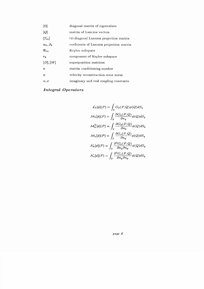
Integral Operators
f-k[0l P) =is
Gk P, Q)O Q)dSqS
aGäP, )Mk[0l P)=i q Q)dsq
Sq
Mk [o] P)_I
aGý P, Q)4j Q)dsq
Sp
aGO P,`w)Mo[ýl P) =i O Q)dsq
Sq
Nk [01 P) =a2Gk P) Q)
O Q)dsqs
an önSqp
No[O] P) =a2Go P, Q)
O Q)dsq8n ön
9P
page 8

8/13/2019 Richard Jeans 1992 PhD Thesis
http://slidepdf.com/reader/full/richard-jeans-1992-phd-thesis 9/215

8/13/2019 Richard Jeans 1992 PhD Thesis
http://slidepdf.com/reader/full/richard-jeans-1992-phd-thesis 10/215
2.5 Thin shell formulation............................................................
39
2.5.1 Boundary integral formulation..............................................
40
2.5.2 Edge conditions
............................................................
43
CHAPTER 3. Collocation Method........................................................
45
3.1 Introduction......................................................................
45
3.2 Discretization....................................................................
45
3.2.1 Interpolation...............................................................
45
3.2.2 Local and Curvilinear Axes.................................................
46
3.3 Integration of Weak Singularity...................................................
47
3.4 Integral Operators................................................................
49
3.4.1 Ck Operator...............................................................
49
3.4.2 Mk Operator..............................................................
51
3.4.3 lVk Operator...............................................................
53
3.4.4 Matrix formulation.........................................................
56
3.4.5 Exterior pressure distribution..............................................
57
3.5 Thecomputer code ...............................................................
58
3.6 Numerical results .................................................................58
3.6.1 Radiation from submerged spheres .........................................58
3.6.2 Acoustic scattering from a submerged sphere ...............................59
3.6.3 Acoustic scattering from a submerged spheroid .............................60
3.6.4 Acoustic scattering from a submerged finite cylinder ........................60
CHAPTER 4. Variational Method........................................................
78
4.1 Introduction......................................................................
78
4.2 Weighted Residue Techniques and the Variational Method........................
78
4.2.1 Weighted Residual Galerkin Method........................................
78
4.2.2 Variational Method........................................................
79
4.3 Variational Boundary Integral Formulation.......................................
80
4.4 Numerical Implementation........................................................
81
4.5 Uniqueness of the Numerical Formulation ......................................... 83
4.6 Edge Boundary Conditions.......................................................
84
4.7 Computer Code..................................................................
85
page 10
8/13/2019 Richard Jeans 1992 PhD Thesis
http://slidepdf.com/reader/full/richard-jeans-1992-phd-thesis 11/215
4.8 Numerical Results................................................................
86
4.8.1 Spheroids..................................................................
86
4.8.2 Flat Disk
..................................................................
87
4.8.3 Flat Square Plate..........................................................
91
4.8.4 Terai s Problem............................................................
91
CHAPTER 5. The Superposition Method................................................
110
5.1 Introduction....................................................................
110
5.2 The Superposition Integral......................................................
111
5.3 Uniqueness......................................................................
113
5.4 Numerical Formulation..........................................................
115
5.4.1 Matrix Condition Number.................................................
118
5.4.2 Velocity Reconstruction Error Norm.......................................
119
5.5 Numerical Results...............................................................
120
5.6 Conclusion......................................................................
122
CHAPTER 6. Elasto-Acoustic Problem..................................................
131
6.1 Introduction .................................................................... 131
6.2 Structural Problem..............................................................
131
6.3 Fluid-Structure Interaction Force................................................
135
6.4 Coupled Equation Set...........................................................
136
6.4.1 Fluid Filled and Non Closed Shell Problems...............................
136
6.4.2 Evacuated Closed Shell Problems..........................................
137
6.5 Solution of Coupled Equation Set................................................
138
6.5.1 Structure Variable Methodology...........................................
138
6.5.2 Fluid Variable Methodology...............................................
139
6.6 Eigenvector Reduction of the Elastic Formulation................................
140
6.7 Interpolation....................................................................
142
6.8 Uniqueness and the Coupled Problem............................................
143
6.9 Elastic Thin Plate Problems.....................................................
147
6.10 Numerical Results .............................................................. 149
6.10.1 Cantilever Plate.........................................................
149
6.10.2 Spherical Shell...........................................................
150
page 11

8/13/2019 Richard Jeans 1992 PhD Thesis
http://slidepdf.com/reader/full/richard-jeans-1992-phd-thesis 12/215
CHAPTER 7. Lanczos vectors in elasto acoustic analysis .................................167
7.1 Introduction....................................................................
167
7.2 Lanczos Vectors
.................................................................
168
7.3 Fluid Variable Methodology.....................................................
171
7.4 Added Fluid Mass Methodology.................................................
172
7.5 Results..........................................................................
173
CHAPTER 8. Conclusions and Recomendations.........................................
191
8.1 Conclusions.....................................................................
191
8.2 Recomen dations .................................................................193
REFERENCES..........................................................................
195
APPENDIX 1 Symmetry and Half Space Problems.......................................
200
A1.1 Image Sources..................................................................
200
A1.2 Geometric Symmetries.........................................................
201
APPENDIX 2 Analytical Solutions......................................................
205
A2.1 Rigid Sphere
...................................................................
205
A2.2 Asymptotic Solutions...........................................................
210
A2.3 Elastic Sphere..................................................................
213
page 12
8/13/2019 Richard Jeans 1992 PhD Thesis
http://slidepdf.com/reader/full/richard-jeans-1992-phd-thesis 13/215
Figures
Page
CHAPTER2
2.1 Geometry for evaluating the discontinuity of the integral operator ..................31
2.2 Geometry for evaluating the surface Helmholtz integral equations .................33
2.3 Non-uniqueness of single layer distribution.........................................
40
2.4 Non-uniqueness of double layer distribution........................................
41
2.5 The thin shell geometry ...........................................................42
CHAPTER 3
3.1 Geometry of the 9-noded isoparametric element ....................................47
3.2 Element sub-division for singular integration.......................................
49
3.3 Geometry for evaluating the far field pressure distribution.........................
58
3.4 The different mesh geometries for the spherical problem ...........................62
3.5-6 Normalized modal impedance for the rigid sphere, 6 elements ................... 63-64
3.7-8 Normalized modal impedance for the rigid sphere, 24 elements ..................65-66
3.9-10 Normalized error of modal impedance..........................................
67-68
3.11 Plane wave backscattered form function for the rigid sphere vs frequency...........
69
3.12-13 Far field form function distribution for scattering by a rigid sphere ..............70-71
3.14 Surface pressure distribution for scattering by a rigid sphere .......................72
3.15 Far field pressure distribution for scattering by a rigid prolate spheroid .............73
3.16 Far field pressure distribution for scattering by a rigid oblate spheroid ..............74
3.17 The different mesh geometries for the cylindrical problem ..........................75
3.18 Far field pressure distribution for scattering by a rigid cylinder .....................76
3.19 Convergence of the far field scattering distribution for a rigid cylinder ..............77
CHAPTER4
4.1 Subelement division...............................................................
82
4.2 Graph of matrix assembly and factorization times.................................
88
page 13

8/13/2019 Richard Jeans 1992 PhD Thesis
http://slidepdf.com/reader/full/richard-jeans-1992-phd-thesis 14/215
4.3 Convergence of backscattered form function for the rigid sphere ....................92
4.4 Convergence of backscattered form function for the rigid prolate spheroid ..........93
4.5 Convergence of backscattered form function for the rigid oblate spheroid ........... 94
4.6 Open plate mesh geometries .......................................................95
4.7 8 Radial pressure amplitude on a circular disk using the variational method .......96 97
4.9 10 Radial pressure amplitude on a circular disk using the collocation method .......98 99
4.11 12 Radial pressure phase on a circular disk using the variational method .........100 101
4.13 14 Radial pressure phase on a circular disk using the collocation method .........102 103
4.15 16 Radiation impedance of a circular disk vs frequency..........................
104 105
4.17 Convergence of radial pressure amplitude on a circular disk.......................
106
4.18 19 Radiation impedance of a square plate vs frequency..........................
107 108
4.20 Near field pressure gain for a point source wave scattered by a rectangular plate. ..109
CHAPTER 5
5.1 The geometry for formulating the superposition integral..........................
112
5.2 The effect of the hybrid formulation on the single and double layer formulations...
124
5.3 Far field backscattering for a sphere using the superposition method ..............125
5.4 Far field backscattering for a spheroid using the superposition method ............126
5.5 The variation of error vs retraction of source surface for the sphere ................127
5.6 The variation of condition nuber vs retraction of source surface ...................128
5.7 The far field error vs retraction of source surface for the spheroid
.................
129
5.8 The velocity error norm vs retraction of source surface surface for the spheroid ....130
CHAPTER 6
6.1 Representation of plate problem ..................................................148
6.2 Cantilever plate geometry ........................................................153
6.3 Far field radiated pressure from point excited fluid filled elastic sphere using the varia
tional method .................................................................... 155
6.4 Far field radiated pressure from point excited fluid filled elastic sphere using the collo
cation method ...................................................................156
page 14

8/13/2019 Richard Jeans 1992 PhD Thesis
http://slidepdf.com/reader/full/richard-jeans-1992-phd-thesis 15/215
6.5 Far field backscattered form function for a fluid filled elastic sphere using the variational
method 1.57
6.6 Far field backscattered form function for a fluid filled elastic sphere using the collocation
method ..........................................................................158
6.7 Far field backscattered form function for a fluid filled elastic sphere using the collocation
Burton and Miller formulation...................................................
159
6.8 The surface pressure and velocity distributions at the first Dirichlet frequency for the
evacuated sphere .................................................................160
6.9 The surface pressure and velocity distributions at the first Neumann frequency for the
evacuated sphere .................................................................161
6.10 The surface pressure and velocity distributions at the first Neumann frequency for the
fluid filled sphere.................................................................162
6.11-12 Far field radiated pressure from point excited fluid filled elastic sphere using the collo-
cation method and frequency interpolation...................................
163-164
6.13-14 Far field radiated pressure from point excited fluid filled elastic sphere using the varia-
tional method and frequency interpolation .................................... 165-166
CHAPTER 7
7.1-4 Velocity response for n=0,1,2 and 3 excitation of a submerged spherical shell using
Lanczos vector reduction of the `dry structural response, and the collocation Burton
and Miller formulation.......................................................
180-183
7.5-8 Velocity response for n=0,1,2 and 3 excitation of a submerged spherical shell using
eigenvector reduction ofthe `dry
structuralresponse, and the collocation Burton
andMiller formulation
...........................................................184-187
7.9 Fluid added mass methodology with Lanczos reduction applied to the far field radiated
pressure of a point excited fluid filled spherical shell ...............................188
7.10 Far filed backscat. tered form function for an evacuated spherical shell with different
hysteretic damping...............................................................
189
APPENDIX 1
A1.1 Image source construction to model infinite rigid plane ...........................200
A1.2 Summary of image source for the acoustic problem ...............................204
page 15
8/13/2019 Richard Jeans 1992 PhD Thesis
http://slidepdf.com/reader/full/richard-jeans-1992-phd-thesis 16/215
APPENDIX 2
A2.1 Plot of the first four spherical Bessel s functions and their derivatives.............
208
A2.2 Geometry for the spheroidal Kirchoff problem .................................... 212
page 16
8/13/2019 Richard Jeans 1992 PhD Thesis
http://slidepdf.com/reader/full/richard-jeans-1992-phd-thesis 17/215
Tables
Page
CHAPTER 4
4 1 Order of Gauss integration 83
4 2 Comparison of accuracy with different orders of integration 87
4 3 Comparison of matrix assembly and factorization times 88
CHAPTER 6
6 1 Comparison
of submerged andin
vacuo quantitiesfor the
cantilever plate153
6 2 Comparison of submerged and in vacuo quantities for the evacuated spherical shell 154
CHAPTER 7
7 1 The percentage accuracy of the modal surface velocity for the fluid variable methodology
with 6 elements and Lanczos reduction of the dynamic structural matrix 176
7 2 The percentage accuracy of the modal surface velocity for the fluid variable methodology
with 24 elements and Lanczos reduction of the dynamic structural matrix 177
7 3 The percentage accuracy of the modal surface velocity for the fluid variable methodology
with 6 elements and eigenvector reduction of the dynamic structural matrix 178
7 4 The percentage accuracy of the modal surface velocity for the fluid variable methodology
with 24 elements and eigenvector reduction of the dynamic structural matrix 179
APPENDIX 2
A2 1 The resonant frequencies for the interior spherical Dirichlet and Neumann acoustic
problems 209
page 17

8/13/2019 Richard Jeans 1992 PhD Thesis
http://slidepdf.com/reader/full/richard-jeans-1992-phd-thesis 18/215
Introduction.
CHAPTER 1.
Introduction
1.1 Background
The acoustic analysis of submerged three dimensional structures is of great interest to en-
gineers. Such an elasto-acoustic analysis can be applied to a variety of engineering problems;
for example the determination of the sound fields generated by aircraft or underwater vehicles
and the design of transducers and acoustic shielding. The potential theory behind the acoustic
problem is also directly applicable to elasto-statics, electromagnetism, hydrodynamics, inviscid
flow and so on. In general the analysis involves solving the dynamic structural response simul-
taneously with the acoustic response, where the two are coupled by a fluid structure interaction.
Standard texts in acoustics e.g. Junger and Feit [1986], Pierce [1989]) present well estab-
lished analytical solutions for simple structures. Morse and Feshbach [1953] list eleven coordinate
systems which allow analytical treatment and Kellog [1929] presents the classical theory behind
such analysis.Early
workin
acoustics concentrated on such analytical results.As
an example
Wiener [1951] published results for thin plate problems and Spence and Granger [1951] presented
analytical results for rigid spheroids.
However analytical results are restricted to a narrow range of geometries. For the vast
majority of realistic problems, a closed form analytical solution does not exist. Before the advent
of digital computers, experimental testing and asymptotic approximations were the only analysis
tools available for arbitrary structures. The availability of high speed computers meant that
complex acoustic problems could be solved efficiently and accurately using numerical methods.
The finite element method FEM) is recognized as a extremely powerful analytical tool
that can be used to solve most well defined continuum problems. It is strongly associated with
structural analysis, but its application to other areas is wide spread. Consequently it was only
natural that it should be applied to the full elasto-acoustic problem and indeed much work has
been done in that area. A modern application of the FEM in acoustics is given by Pinsky and
Abboud [1990], who consider the transientanalysis of
theexterior
acoustics problem.
A FEM analysis of the acoustic problem is hampered by a number of difficulties. The acous-
tic problems of greatest interest are often those involving a fluid of infinite extent. Discretization
page 18

8/13/2019 Richard Jeans 1992 PhD Thesis
http://slidepdf.com/reader/full/richard-jeans-1992-phd-thesis 19/215
Introduction.
of such a fluid domain for the FEI is obviously difficult and almost always unsatisfactory. Even
with the use of infinite elements, the resulting equation set is large and cumbersome. Such a
method is inefficient since the variables of most interest are those on the interface between the
fluid and structural domains.
Boundary integral formulations of potential problems have been recognized for a long time.
By using the power of the new digital computers it was quickly recognized that a boundary
element method (BEM) promised an elegant and efficient solution technique for the numerical
analysis of potential problems. Regarding the acoustic analysis of rigid structures, Chen and
Scheikert [1963] published a numerical method based on the boundary layer integral formulation
and a year later Chertock[1964]
published a method based on the Helmholtz integral equation.
Over the last two decades, the BEM has emerged as the preferred solution technique for acoustic
problems in the exterior domain.
The strength of an integral formulation of the acoustic problem is the reduction of di-
mensionality; the three dimensional exterior pressure field is represented by a two dimensional
integral relationship on the surface of the structure. The elegance of the method is the math-
ematical simplicity of the resulting integral expressions. However, it was recognized by Lamb
[1945] that there is a difficulty with the classical integral formulations. At the standing wave
frequencies of the interior domain defined by the structural surface, the integral equations for
the exterior problem fail to provide a unique solution. The numerical consequences of this non-
uniqueness for rigid acoustic problems was examined by Copley [1967] and the first improved
numerical formulation to circumvent the problem was presented by Schenck [1968]. Burton and
Miller [1971] presented a composite integral formulation that was valid at all wavenumbers.
Kleinman and Roach [1974] as well as Filippi [1977] presented a mathematically rigorous analy-
sis of the uniqueness properties of the various formulations, showing the equivalence between the
boundary layer and Helmholtz integral formulations. The behaviour of BEM s at critical wave
numbers continues to be of interest and recently Dokumaci [1990] discussed the exact nature of
numerical failure of the BEM at these frequencies.
The Burton and Miller formulation and Schenck s Combined Helmholtz Integral Equation
Formulation (CHIEF) still remain today as the main numerical strategies for overcoming prob-
lems of uniqueness, each having it s own strengths and weaknesses. The Burton and Miller
formulation is robust and well tested but necessitates the evaluation of a hypersingular integral.
The CHIEF formulation on the other hand is simpler but fails at higher frequencies and involves
the solution of an over determined system of equations.
page 19

8/13/2019 Richard Jeans 1992 PhD Thesis
http://slidepdf.com/reader/full/richard-jeans-1992-phd-thesis 20/215
Introduction.
The first boundary element analyses were concerned with either a prescribed surface velocity
distribution or rigid body scattering. Zienkiewti cz Kelly and Bettess [1977] presented an analysis
of the general coupling between a FE-N1and BENZ derived from the FEM point of view. It was
Wilton [1978] who first showed the feasibility of coupling a structural finite element formulation
and an acoustic boundary element formulation.
Boundary integral and finite element formulations can often be applied to the same set of
problems and are often perceived as competing solution techniques. However the two method-
ologies have complementary strengths and weaknesses and their combination often results in
a very powerful solution technique. In the elasto-acoustic problem the FEM is best suited to
the accurate determination of the localized structural problem and the BEM is best suited to
the fluid problem of infinite extent. Not only do fluid-structure interaction problems suit this
category of analysis but so do a large number of other engineering problems; e.g. structure-soil
interaction structural non-linearities within homogeneous structures and so on.
A large proportion of published boundary integral formulations use constant interpolation
of the fluid variables. A popular interpolation technique uses the concept of a superparametric
element as used by Wilton [1978] and recently in the field of electro-magnetism by Ingber and
Ott [1991]. Within the superparametric element the level of geometric interpolation is higher
than the level of fluid interpolation. Mathews [1979][1986] introduced isoparametric interpola-
tion common in the FEM where both the fluid and geometric variables are interpolated by
quadratic Lagrange shape functions. Amini and Wilton [1986] implement a number of different
interpolation schemes to show the advantages in convergence efficiency and accuracy possible
with quadratic interpolation of the fluid variables.
Mariem and Hamdi [1987] presented a new variational formulation of the BEM for the thin
shell problem. In this formulation based on the work of Maue [1949] and Stallybrass [1967]
the kernel of the hypersingular integral operator is transformed using tangential derivatives
and then integrated with respect to the field point over the surface of the structure. The
resulting symmetric expression contains only a weak singularity which is amenable to numerical
integration. The disadvantages of the method is the increase in computational time needed for
thesecond
numerical integration.
Despite the advantages there seem to be very few researchers using isoparametric elements.
The variational method is idealy suited to high order fluid interpolation since the reduction
page 20

8/13/2019 Richard Jeans 1992 PhD Thesis
http://slidepdf.com/reader/full/richard-jeans-1992-phd-thesis 21/215
Introduction.
of the singularity is independent of numerical discretization. Of the few published papers us-
ing such interpolation techniques, Coyette and Fyfe [1989] and Jeans and Mathews [1990] used
a variational approach. Isoparametric implementations of the Collocation Burton and Miller
method have been published by Chien, Rajiyah and Atluri [1990] and W a u,Seybert and Wan
[1991]. The work by Chien et al, employed a complicated treatment of the hypersingular inte-
gral operator, dependent on the exact form of interpolation, \Vu et al employed the tangential
formulation given by Maue and then used additional regularization to integrate the remaining
Cauchy type singularity. Seybert and his co-workers have published a number isoparametric
implementations of the CHIEF methodology; e.g. Seybert, Soenarko, Rizzo and Shippy [1985].
Such
an
implementation is aided by the absence of a hypersingular integral operator, but suffers
from the inherent problems of the CHIEF methodologies.
It has already been mentioned that a large amount of research effort has been involved in
the question of the uniqueness of the integral formulation at critical frequencies. This work is
primarily on the BEM in isolation from the coupled elasto-acoustic formulation. The CHIEF and
Burton and Miller techniques seem to have been included in the coupled formulations without
qualification, although the fact that the structural formulation does not remove the ill condi-
tioning of the numerical formulation at the critical frequencies is not, in general, immediately
obvious. Huang [1984] attempted to clarify the situation by explicitly showing the theoretical
non-uniqueness at the critical frequencies of the unrelated internal acoustic problem. However
he also stated that in reality this non-uniqueness will not be present. Although this was true for
the constant fluid basis functions he was using, Mathews [1986] disproved Huang s conjecture
for isoparametric implementations of the elasto-acoustic BEM.
Like the Burton and Miller formulation, the acoustic problem of thin plates and shells has
been hampered by the need to numerically approximate the hypersingular integral operator.
A large amount of successful numerical work in this area has been published by Pierce and
colleagues; e.g. Pierce [1987], Wu, Pierce and Ginsberg [1987] and Ginsberg, Chen and Pierce
[1990]. This work used the Helmholtz intergal equation and variational procedures, but also
used axisymmetric basis functions based on an a priori understanding of the problem. Terai
[1980] applied his BEM to thin plate problems as did Coyette and Fyfe [1989], however the
approach of Coyette and Fyfe ultimately lead to the assumption of incompressible fluid to
facilitate an eigenmode analysis. Recently Kirkup [1991] has modeled the effects of acoustic
shields using a coupled FEM/BEM, but in general there seems to be little published work into
page 21

8/13/2019 Richard Jeans 1992 PhD Thesis
http://slidepdf.com/reader/full/richard-jeans-1992-phd-thesis 22/215
Introduction.
the application of BEM s to unbaffled thin plate problems of arbitrary geometry and even less
using isoparametric interpolation.
Without any simplifying approximations using a BEM to model the effect of the fluid on
a submerged structure leads to a non-linear eigenvalue problem. The simplest approach to a
dynamic analysis of such a structure, involves an analysis at a large number of frequency points.
The computational bottle-necks for this approach are the evaluation of the fluid impedance ma-
trix relationship at each frequency, and the large number of degrees of freedom in the structural
equation set. Wilton [1978] recognized the second of these problems and reduced the dynamic
structural matrix using the `dry eigenmodes. The problem of calculating the fluid impedance
matrix at a large number of frequency points is alleviated by frequency interpolation. Kirkup
and Henwood [1989], Schenck and Benthien [1989] and Benthien [1989] all presented and evalu-
ated interpolation techniques and Schenck and Benthien [1989] discussed in general the problems
of applying coupled BEM/FEM techniques to large scale elasto-acoustic problems. The use of
such interpolation schemes can also facilitate a modal analysis of the fluid structure interaction
problem (Kirkup and Amini [1990]). Recently Lanczos and Ritz vector techniques have been
applied to the internal fluid structure interaction problem (Moini, Nour-Omid and Carlsson
[1990], Coyette [1990]), and their use in the coupled BEM/FEM formulations promises signifi-
cant advantages over modal reduction (Jeans and Mathews [1991]).
Overcoming the problem of the hypersingular integral operator present in both Burton
and Miller and thin shell acoustic formulations, represents a large amount of research effort.
Over the years many solutions to the problem have been suggested along with an unavoidable
increase in the computational complexity of the implementation. Cunefare and Koopmann [1989]
presented a methodology they called CHI (Combined Helmoltz Integrals), where the problem
is circumvented by constraining all the field points to be interior to the surface. Koopmann,
Song and Fahline [1989] proposed a wave superposition method, where the surface pressure
distribution was reconstructed from a source distribution interior to the surface of the radiator.
Recently there has been some favorable interest in this method, with Miller, Moyer, Huang
and tTberall [1991] looking at the coupling of the FEM and Superposition method, and Song,
Koopmann and Falinline [1991] investigating the associated numerical errors.
All researchers to date recognize the problems with the retraction of the source surface in
order to circumvent high order singularities; i.e. the inherent numerical difficulties of discretizing
Fredholm integral equations of the first kind (Miller [1974]). The interior source or field points
need to be chosen carefully in order to obtain sufficiently well conditioned numerical systems.
page 22

8/13/2019 Richard Jeans 1992 PhD Thesis
http://slidepdf.com/reader/full/richard-jeans-1992-phd-thesis 23/215
Introduction.
Many researchers, including the author, believe that the superposition method is simply an
ill-conditioned form of the BEM, and singularities in the integral equations are an unavoidable
consequence of optimizing the numerical robustness and conditioning of the problem. This is
the motivation behind a recently submitted paper (Jeans and Mathews [1991]).
1.2 Motivation of Present Thesis
The original motivation for this thesis was to develop and refine the current state of the
art computational approaches used for the prediction of radiated sound. After three years of
research the following areas have been documented in this thesis:
(a) Development of a computationally efficient implementation of the Helmholtz in-
tegral equations for three dimensional structures of arbitrary geometry, including
thin plate problems.
i) Comparison and development of variational and collocation formulations.
ii) The use of quadratic isopararnetric elements.
iii) Frequency interpolation of fluid matrices.
(b) Coupling of a consistent FEM formulation of the thin shell and plate structural
problem to the boundary element formulations.
i) Comparison of modal and Lanczos reduction of the structural formula-
tions to improve solution efficiency.
A general review of the acoustic problem, along with the development of the various integral
formulations, is given in Chapter 2. In Chapter 3a collocation approach is presented for the
numerical solution of the Burton and Miller formulation of the exterior acoustic problem. This
work describes a novel approach to the hypersingular integral operator, based on the expression
of the integral operator given by laue [1949]. This approach is very similar to the work of Wu,
Seybert and Wan [1991], but without their additional regularization procedures. The resulting
numerical implementation is applied to spherical, spheroidal and cylindrical rigid radiation and
scattering problems.
In Chapter 4 the variational method of Mariem and Hamdi [1987] for approximation of
the hypersingular integral operator is described and numerically implemented using quadratic
isoparametric boundary elements. The resulting thin shell acoustic formulation is applied to
page 23
8/13/2019 Richard Jeans 1992 PhD Thesis
http://slidepdf.com/reader/full/richard-jeans-1992-phd-thesis 24/215
Introduction.
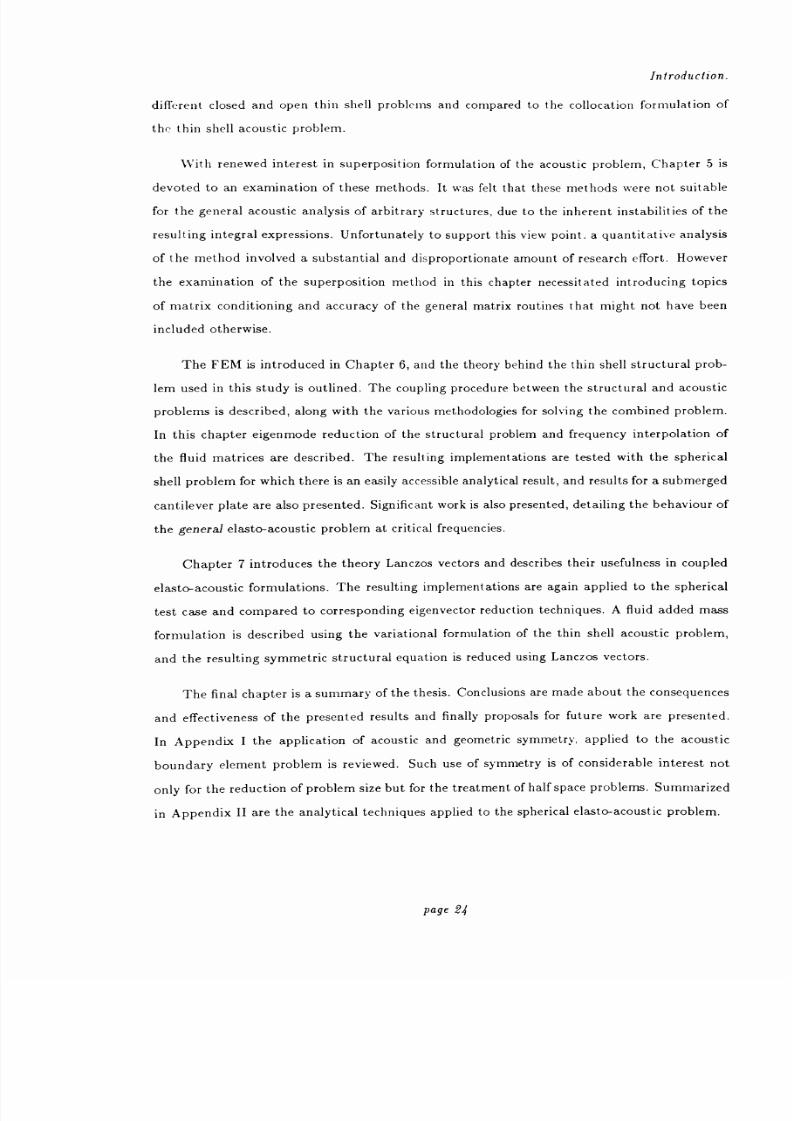
different closed and open thin shell problems and compared to the collocation formulation of
the thin shell acoustic problem.
With renewed interest in superposition formulation of the acoustic problem Chapter 5 is
devoted to an examination of these methods. It was felt that these methods were not suitable
for the general acoustic analysis of arbitrary structures due to the inherent instabilities of the
resulting integral expressions. Unfortunately to support this view point a quantitative analysis
of the method involved a substantial and disproportionate amount of research effort. However
the examination of the superposition method in this chapter necessitated introducing topics
of matrix conditioning and accuracy of the general matrix routines that might not have been
included otherwise.
The FEM is introduced in Chapter 6 and the theory behind the thin shell structural prob-
lem used in this study is outlined. The coupling procedure between the structural and acoustic
problems is described along with the various methodologies for solving the combined problem.
In this chapter eigenmode reduction of the structural problem and frequency interpolation of
the fluid matrices are described. The resulting implementations are tested with the spherical
shell problem for which there is an easily accessible analytical result and results for a submerged
cantilever plate are also presented. Significant work is also presented detailing the behaviour of
the general elasto-acoustic problem at critical frequencies.
Chapter 7 introduces the theory Lanczos vectors and describes their usefulness in coupled
elasto-acoustic formulations. The resulting implementations are again applied to the spherical
test case and compared to corresponding eigenvector reduction techniques. A fluid added mass
formulation is described using the variational formulation of the thin shell acoustic problem
and the resulting symmetric structural equation is reduced using Lanczos vectors.
The final chapter is a summary of the thesis. Conclusions are made about the consequences
and effectiveness of the presented results and finally proposals for future work are presented.
In Appendix I the application of acoustic and geometric symmetry applied to the acoustic
boundary element problem is reviewed. Such use of symmetry is of considerable interest not
only for the reduction of problem size but for the treatment of half space problems. Summarized
in Appendix II are the analytical techniques applied to the spherical elasto-acoustic problem.
page 24

8/13/2019 Richard Jeans 1992 PhD Thesis
http://slidepdf.com/reader/full/richard-jeans-1992-phd-thesis 25/215
. acoustic Problem.
CHAPTER 2.
Acoustic Problem
2.1 Fundamental Equations
The analysis of any acoustic problem involves the solution of a differential equation relating
fluid variables in the medium of interest, subject to certain boundary conditions. This work is
primarily concerned with the interaction of acoustic radiation with submerged structures and
the appropriate differential equation is the linear wave equation subject to a velocity boundary
condition on the submerged structure.
2.1.1 Linear Approximation
In a fundamental analysis (Pierce [1989]) of the acoustic pressure field, the linear wave
equation is developed from a consideration of mass and energy conservation. This analysis
assumes that the acoustic pressure field is a small amplitude perturbation to the ambient state,
characterized by those values that pressure, density and fluid velocity have when the perturbation
isabsent.
The fluidor acoustic medium
isassumed
to be homogeneousand quiescent;
ie the
ambient quantities are assumed to be independent of position and time with the ambient fluid
velocity equal to zero.
Consider a body of fluid in a volume V, with density p, surrounded by a surface S. The
fluid velocity at a point P is given by v(P) and the outward normal to the surface S is defined
by n. Conservation of mass requires that the net mass leaving V per unit time is equal to the
rate at which mass decreases in V. This is expressed by the relationship,
-
dt
JpdV =J pv ndS.
vs
(2.1.1)
The right hand side of this equation can be transformed to a volume integral by means of Gauss'
theorem and Euler's differential equation for conservation of mass is obtained,
a
alp 17-(Pvv)=o.
(2.1.2)
The pressure field at a point P is given by p(P). By considering the forces acting on the
fluid, and neglecting body forces and viscosity, the fluid velocity and pressure are related by,
page -95

8/13/2019 Richard Jeans 1992 PhD Thesis
http://slidepdf.com/reader/full/richard-jeans-1992-phd-thesis 26/215
Acoustic Problem.
p(av
+ (v V)v
This equation represents an example of Reynolds' transport theorem.
The relationship between the pressure field and density in the fluid is obtained by making the
assumption that the acoustic radiation is adiabatic in the linear approximation. Consequently
it is possible to write,
aP 2aP2_(ap),
(9t (9t ap
(2.1.4)
The real constant c is refered to as the speed of sound in the particular fluid medium and
the subscript s in Eq. (2.1.4),
indicates that the differential is evaluated at constant entropy.
Writing the pressure, density and velocity as small perturbations of the ambient state,
P=Po+p, P=Po+Pý, v=v'. (2.1.5)
the linear differential equations governing these perturbations are defined as,
op i+c2po0 - v' = 0, (2.1.6)
öv'VP'+po = 0.
2.1.2 Wave Equation
The wave equation results when v' is eliminated from Eq. (2.1.6) and Eq. (2.1.7).
From
now on the prime notation will be neglected when indicating ambient state perturbations. The
wave equation is given by,
v2pla2P
_-o.2 öt2(2.1.8)
page 26

8/13/2019 Richard Jeans 1992 PhD Thesis
http://slidepdf.com/reader/full/richard-jeans-1992-phd-thesis 27/215
Acoustic Problem.
Since the fluid velocity and pressure are given by a linear differential equation, it is possible
to assume an harmonic time dependency of the form e-' t, where ,;is the circular frequency of
the pressure field. The time independent fluid variables are,
p= Pe-iwt v= ive cwt. (2.1.9)
Substituting Eq. (2.1.9) into Eq. (2.1.8) results in the expression,
V2p+k2p= 0. (2.1.10)
where the wave number k is w/c. This equation is known as the reduced wave equation or
Helmholtz' equation.
2.1.3 Neumann boundary condition
The reduced wave equation is solved in terms of the Neumann boundary condition which
relates the fluid velocity to the normal velocity prescribed on S. This boundary condition is
defined by,
Op-n -
iwpvr,, (2.1.11)
where the subscript notation for the ambient density, p, is dropped and,
ap_n _n V , vn =nýv. (2.1.12)
This boundary condition is sufficient for the solution of Helmholtz' equation for a finite
body of fluid. For unbounded fluid problems another boundary condition is needed to uniquely
specify the solution to Helmholtz' equation.
2.1.4 Sommerfeld's radiation condition
For unbounded acoustic problems the pressure field must obey some boundary condition
in the far field. This boundary condition is given by Sommerfeld's radiation condition. This is
defined by,
page 27
8/13/2019 Richard Jeans 1992 PhD Thesis
http://slidepdf.com/reader/full/richard-jeans-1992-phd-thesis 28/215
4coustic Problem.
lien
Jkp dS=0 (2.1.13)
r--co S
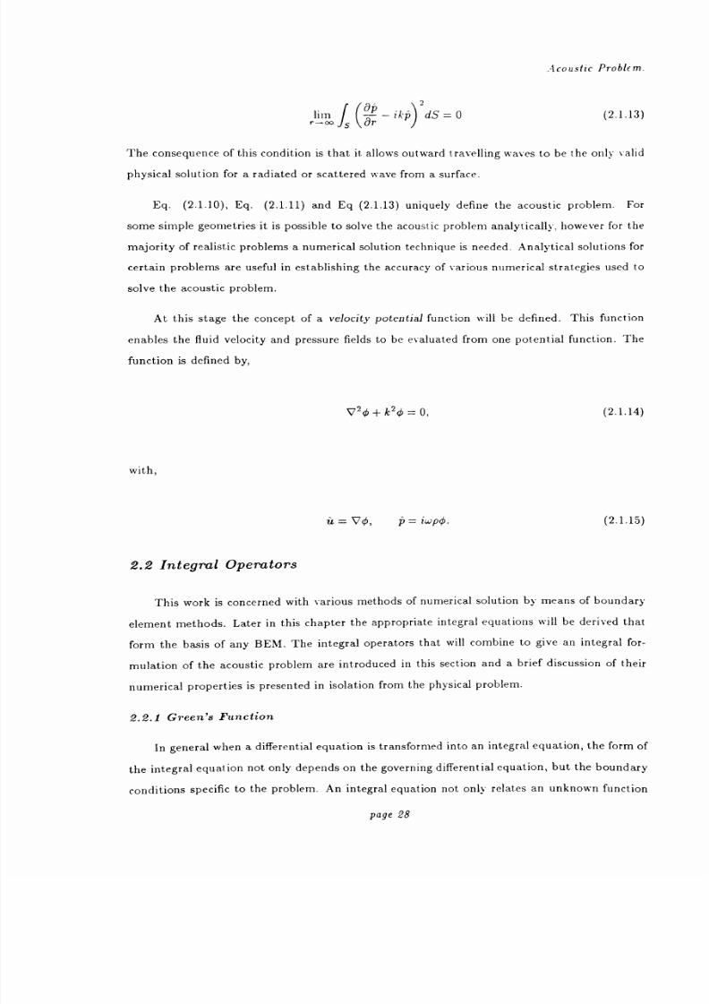
The consequence of this condition is that it, allows outward travelling waves to be the only valid
physical solution for a radiated or scattered wave from a surface.
Eq. (2.1.10), Eq. (2.1.11) and Eq (2.1.13) uniquely define the acoustic problem. For
some simple geometries it is possible to solve the acoustic problem analytically, however for the
majority of realistic problems a numerical solution technique is needed. Analytical solutions for
certain problems are useful in establishing the accuracy of various numerical strategies used to
solvethe
acoustic problem.
At this stage the concept of a velocity potential function will be defined. This function
enables the fluid velocity and pressure fields to be evaluated from one potential function. The
function is defined by,
020 + 120 = 0, (2.1.14)
with,
ü= VO, p= iwpq. (2.1.15)
2.2 Integral Operators
This work is concerned with various methods of numerical solution by means of boundary
element methods. Later in this chapter the appropriate integral equations will be derived that
form the basis of any BEM. The integral operators that will combine to give an integral for-
mulation of the acoustic problem are introduced in this section and a brief discussion of their
numerical properties is presented in isolation from the physical problem.
2.2.1 Green s Function
In general when a differential equation is transformed into an integral equation, the form of
the integral equation not only depends on the governing differential equation, but the boundary
conditions specific to the problem. An integral equation not only relates an unknown function
page 28

8/13/2019 Richard Jeans 1992 PhD Thesis
http://slidepdf.com/reader/full/richard-jeans-1992-phd-thesis 29/215
.Acoustic Problem.
to its derivatives; ie values at neighbouring points, but also to its values at the boundary. The
boundary conditions are built into an integral equation through the form of its kernel, but for
a differential equation the boundary conditions are imposed at the final stage of solution. This
kernel is the Green s function for the problem.
For the acoustic problem, the Green s function is the fundamental solution of the inhomo-
geneous Helmholtz equation,
(02+ k2)GkP,Q)= -6(P,Q), (2.2.1)
where 6(P, Q) is the delta-dirac function. Also the Green s function must satisfy Sommerfeld*s
radiation condition, Eq. (1.1.13). The appropriate solution in three dimensions is given by,
Gk(P) Q) -
ikr
4 rr= JP- Qj. (2.2.2)
In this equation r is the Euclidean distance between the field points P and Q.
2.2.2 Discontinuities
The integral operators that are of interest are defined by,
,Ck01(P) =
isGk (1 )Q)O(Q)dSq, (2.2.3)
s
Mk[c](P) _öG9 P, Q)
q(Q)dSq, (2.2.4)S4
Mk0](P)s
GäP, )O(Q)dSq, (2.2.5)
Sp
Ar [0)(ý ) =a2Gk(P, Q)
0(Q)dSq. (2.2.6)Sananp
The function 0 is assumed to be a continuous function over S. For completeness there is also
the identity operator,
1[01(p) = «(P). (2.2.7)
An important property of these operators defined in Eq. (2.2.3-6) is that they are all solutions of
the original acoustic differential equation. Each can be thought of as the result of a continuous
distribution of sources, magnitude O(Q), over the surface of S.
page 29

8/13/2019 Richard Jeans 1992 PhD Thesis
http://slidepdf.com/reader/full/richard-jeans-1992-phd-thesis 30/215
Acoustic Problem.
It is useful to establish the behaviour of these integral operators as the field point P is
brought to the surface S. The limit of a field point brought to the surface in the direction
opposite to the direction of the surface normal will be denoted by p+, the limit of the field point
brought to the surface in the same direction as the surface normal will be denoted by p- .In
general points on a surface will be denoted by lower case symbols. Firstly construct a small
sphere of small radius e centered around the surface limit point. The domain of integration is
taken to be the surface S, excluding the small sphere, and that part of the small sphere, S£,
that completes the surface. The radius e is then taken to zero to evaluate the limiting value of
the integral operator. Figure (2.1) illustrates the geometry for evaluating the limit of P -- p+.
Consider the integral operator Ck.
lm,Ck[O)(P) =1ö Gk(p, 4)4(4)dSq +J
4ýesin(B)dOdyh .(2.2.8)
[IS-S, rz
P P+ S.
The polar angles 0 and 0 define the surface S. For Eq. (2.2.8) the second term on the right
hand side goes to zero in the limit and so the operator Gk is continuous across the surface S.
Consider the same limiting process for the.
Mk operator,
I aGk(n,) 2Pm Mk[01(P) = li ö anO(4)dsq+ 4ýý2 ýsin(8)d6d¢ (2.2.9)
P+ _Sc 4
Is
t
In Eq. (2.2.9) the vector r is the unit vector pointing from P to p+. This time the second term
on the right hand side tends towards a limiting value and so,
lim A4k[O](P) _ Mk[Q](P) + (l - c(P))O(P) (2.2.10)P-4p+
The quantity 4irc(p) is the external solid angle at the point p. For a smooth surface; ie one that
has a unique tangent plane, then
1c(P) =2
A definition of c(p) can be gained by considering the limit,
(2.2.11)
page 30

8/13/2019 Richard Jeans 1992 PhD Thesis
http://slidepdf.com/reader/full/richard-jeans-1992-phd-thesis 31/215
Acoustic Problem.
n
P048440 ...
Sc
P p+
p-
q
SE
Figure 2.1). Geometry for evaluating the discontinuity of the integral operators.
page 31

8/13/2019 Richard Jeans 1992 PhD Thesis
http://slidepdf.com/reader/full/richard-jeans-1992-phd-thesis 32/215
Acoustic Problem.
Jim-PPI
aGo(P q)dS(2.2.12)
P-P+ ,
This equation is continuous as P passes through the surface S. Noting the discontinuity in the
Mk operator, indicates a mathematical definition for the quantity c(p),
aco(p,)ds(P) =1+f an qSq
(2.2.13)
Using the arguments described above, it is possible to evaluate the discontinuity properties
of all the integral equations and these are summarized below,
4 [OI P+) _ ck [OI P)-
4[0](P -)i (2.2.14)
Mk [c](P+)-
(1- c(P))q(P) _ Mk [01(P) = Mk [Q](P )+ c(P)O(P), (2.2.15)
k[o](p+) + (1
- C(P))O(p) _k [o](P) = Mk [©](p-)- C(P)4(P), (2.2.16)
Nk[0l (P+)= Nk[¢](P)= Nk[q](p ), (2.2.17)
It is important to realize that Mk[q](p+) represents the limiting value of Mk[O](P) as P
tends to p+, whilst Mk [O](p) represents the principal value of the integral operation; that is the
limit value of an integration over a surface S-S,, as 6 goes to zero.
2.3 Helmholtz Integral Equations
2.3.1 Surface Helmholtz Integral Equation
The Surface Helmholtz Integral equation (SHIE) forms the basis of most boundary element
methods (BEM). This equation can be derived by considering the general acoustic geometry
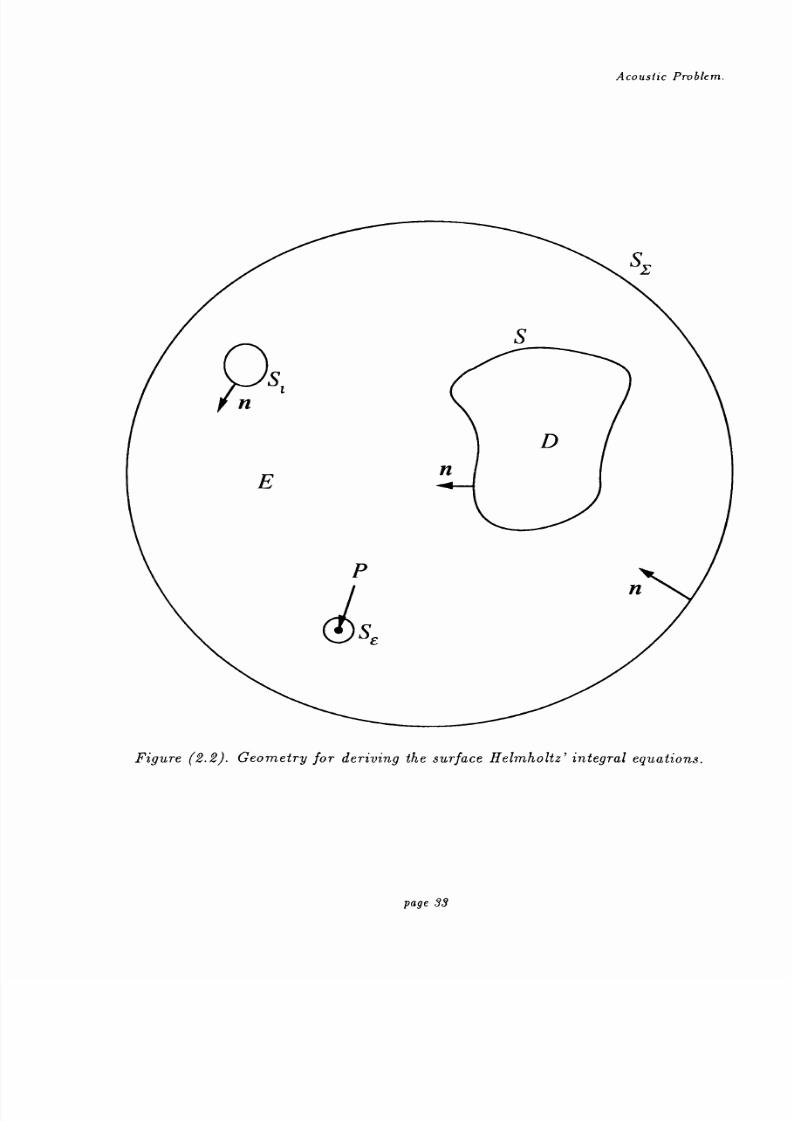
shown in figure (2.2). A spherical surface, Sr, contains two closed surface Si and S. The surface
S represents the acoustic surface of interest and the surface Si represents the surface of some
acoustic source. The domain E is the volume contained by SE excluding the volume contained
by Si and S. The domain D represents the volume contained by the surface S. A small spherical
surfaceSE
surroundsthe field
pointP.
With the surface SE excluding the singular point P from the domain E, both the Green s
free space function and the velocity potential in E satisfy the reduced wave equation and so,
page 32
8/13/2019 Richard Jeans 1992 PhD Thesis
http://slidepdf.com/reader/full/richard-jeans-1992-phd-thesis 33/215
Acoustic Problem.
Figure (2.2). Geometry for deriving the surface Helmholtz integral equations.
page 33
8/13/2019 Richard Jeans 1992 PhD Thesis
http://slidepdf.com/reader/full/richard-jeans-1992-phd-thesis 34/215
,Acoustic Problem.
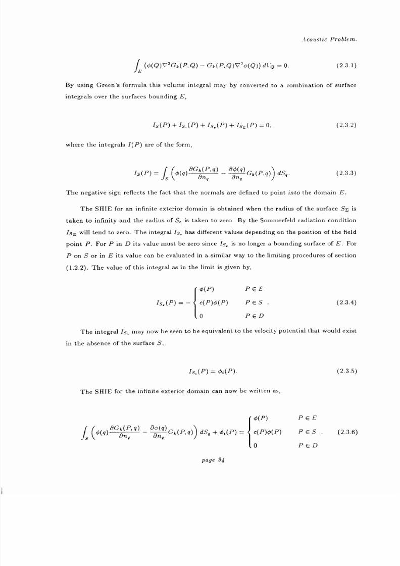
Q=0. (2.3.1)(4(Q)V2Gk(P, Q) - Gk(P, Q)V2o(Q)) dlE
By using Green's formula this volume integral may by converted to a combination of surface
integrals over the surfaces bounding E,
Is(P)+Is. (P)+Is, (P)+Is, (P)_0, (2.3.2)
where the integrals I(P) are of the form,
Is(P) _ O(q)oGk(P, q)
_90(q)
Gk(P, q) dSq. (2.3.3)Sqqq
The negative sign reflects the fact that the normals are defined to point into the domain E.
The SHIE for an infinite exterior domain is obtained when the radius of the surface Sr, is
taken to infinity and the radius of SE is taken to zero. By the Sommerfeld radiation condition
IS. will tend to zero. The integral Is has different values depending on the position of the field
point P. For P in D its value must be zero since IS,, is no longer a bounding surface of E. For
P on S or in E its value can be evaluated in a similar way to the limiting procedures of section
(1.2.2). The value of this integral as in the limit is given by,
O(P) PEE
Is, (P) c(P)¢(P) PES.
(2.3.4)
0 PED
The integral IS, may nowbe
seen tobe
equivalentto the
velocity potentialthat
would existin the absence of the surface S,
Is, (P) = Oi(P).
The SHIE for the infinite exterior domain can now be written as,
O(P)
o(q)0Gk(P, q)
_ao(q)
Gk(p, q) dS9+ Oi(P) _ c(P)O(P)an, Önqt0
PEE
PES
(2.3.5)
(2.3.6)
PED
Page 94

8/13/2019 Richard Jeans 1992 PhD Thesis
http://slidepdf.com/reader/full/richard-jeans-1992-phd-thesis 35/215

8/13/2019 Richard Jeans 1992 PhD Thesis
http://slidepdf.com/reader/full/richard-jeans-1992-phd-thesis 36/215
Acoustic Problem.
2.3.3 Boundary Layer Formulations
It was stated in Section 2.2 that the result of the integral operators on a continuous function
defined on the surface S, was a solution of the acoustic wave equation. Further more with the
correct definition of the Green's function the solution satisfies the radiation condition. Conse-
quently it is possible to define the velocity potential in the exterior domain, E. in terms of a
single layer distribution, p,
ö(P) = Ck {c)(P), PEE. (2.3.13)
By differentiating with respect to some normal vector, defined in the exterior domain, an ex-
pression for the dimensionless velocity field is obtained.
aý(P)-. 4[, c](P),np
PEE. (2.3.14)
When the field point, P, is taken to the surface S, the boundary layer formulation for the
acoustic problem is defined by,
[Mk-
(1- c(P))] P, pcS.
on(2.3.15)
Eq. (2.3.15) can be solved to obtain the single layer density p, and then Eq. (2.3.13) can be
used to evaluate the exterior and surface velocity potentials.
In a similar way the exterior velocity potential can be defined in terms of a double layer
distribution, a,
0 (P) _ . k[O](P)7PEE. (2.3.16)
The differentiated form is given by,
a¢(P)
- JVk[0](P),PEE. (2.3.17)
önp
Since the Vk operator is continuous across the surface S, then Eq. (2.3.17) can be solved for
PES and the surface -velocity potential is defined by,
page 36

8/13/2019 Richard Jeans 1992 PhD Thesis
http://slidepdf.com/reader/full/richard-jeans-1992-phd-thesis 37/215
Acoustic Problem.
0= [Mk +(1-C(P))]o.
The exterior velocity potential is given by Eq. (2.3.16).
2.4 Uniqueness of Boundary Integral Formulations
2.4.1 SHIE and DSHIE formulations
(2.3.18)
For given boundary conditions the velocity potential for the exterior problem is unique.
However it has long beenrecognized
thatwhen expressed
in termsof a
boundary integral
formulation the solution to the exterior problem may not be unique. Non-uniqueness of the
solution occurs at critical wavenumbers k, and for the acoustic problem these wavenumbers
correspond to interior resonant frequencies. It needs to be emphasized that this problem of
non-uniqueness does not imply non-uniqueness of a physical solution, but a breakdown of the
theoretical formulation at critical frequencies. A numerical implementation of an unmodified
exterior boundary integral formulation will result in ill-conditioning of the matrices at a range
of
frequencies,
centered aroundthe
critical
frequency.
The problem of non-uniqueness can be illustrated by considering the exterior Neumann
problem, Eq. (2.3.11), for a `smooth surface . There will be a unique solution as long as there
are no non-trivial solutions to the homogeneous equation,
(I+M)v=0. (2.4.1)
The non-trivial solutions to this equation occur at the eigenvalues k,. By the Fredholm Alter-
native theorems, the eigenvalue spectrum of this equation is the same as that of the transpose
Of ,
2Z-}-Mkv = 0. (2.4.2)
The eigenvalues of this equation correspond to the eigenvalues for the unrelated interior Neu-
mann problem, Eq (2.3.9). Simiarly the critical wavenumbers for the exterior Dirichlet problem
correspond to the eigenvalues of the interior Dirichlet problem.
page 37

8/13/2019 Richard Jeans 1992 PhD Thesis
http://slidepdf.com/reader/full/richard-jeans-1992-phd-thesis 38/215
Acoustic Problem.
For all but simple boundary geometries it is impossible to predict the values of kn. There-
fore it is highly desirable to implement a strategy that will eliminate the problem of the ill-
conditioning of the numerical formulation in the region of critical wavenumbers. Several strate-
gies have been proposed all of which unfortunately increase the computational burden of the
problem.
2.4.2 The CHIEF method
One of the first methods proposed to remove the problem of non-uniqueness was that of
Schenck [1968]. In this method the algebraic equations generated from the SHIE are combined
with additional equations generated from the interior Helmholtz relationship,
001Mk [01(P) _ ,
CkOn
(P)- OA(P), PED, (2.4.3)
evaluated at a number of interior points. The resulting overdetermined set of equations can be
solved by a least squares method.
There are several problems with this method. When some of the interior points lie on
nodal surfaces it has been shown that this method may not remove the problem of uniqueness.
Consequently, at high frequencies when the density of interior nodal surfaces is high, the choice
of interior nodal posit-ion is difficult. Several methods for choosing these nodal points have been
proposed but this adds to the complexity of the solution. For an arbitrary selection of interior
points this method cannot be relied on to remove the problem of non-uniqueness.
2.4.3 Burton and Miller s Formulation
Burton and Miller proposed [1971] that the problem of uniqueness could be overcome by
forming a linear combination of the SHIE and DSHIE. This linear combination is given by,
{ [-c(P)Z Mk] + OA k-_{ rk +a [c(P)Z +M]}ý- (Oi +a
örti .(2.4.4
On
I]
Burton and Miller demonstrated that for an imaginary coupling constant a, this formulation
should yield a unique solution for all wavenumbers.
The disadvantage of this formulation is that the kernel of the AVkoperator is highly singular
and a method needs to be used in order to integrate this operator numerically.
page 38
8/13/2019 Richard Jeans 1992 PhD Thesis
http://slidepdf.com/reader/full/richard-jeans-1992-phd-thesis 39/215
acoustic Problfnz.
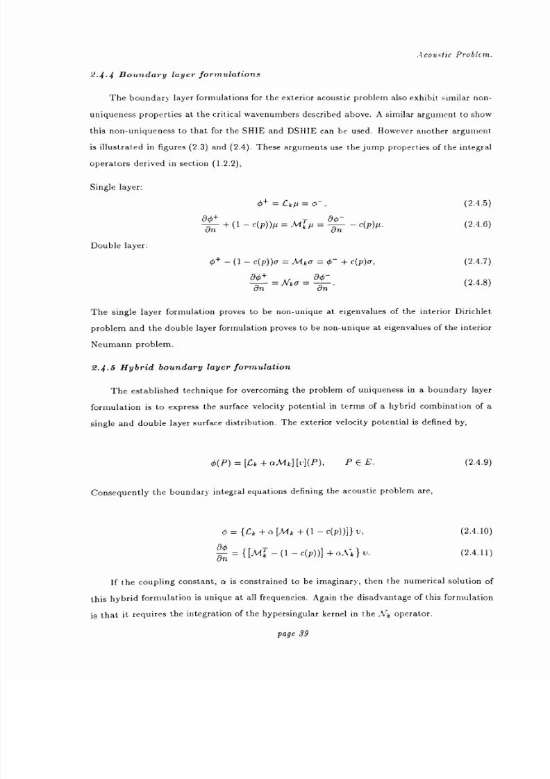
2.4.4 Boundary layer formulations
The boundary layer formulations for the exterior acoustic problem also exhibit similar non-
uniqueness properties at the critical wavenumbers described above. A similar argument to show
this non-uniqueness to that for the SHIE and DSHIE can be used. However another argument
is illustrated in figures (2.3) and (2.4). These arguments use the jump properties of the integral
operators derived in section (1.2.2),
Single layer:
4+ _ ,Ckµ = 4-, (2.4.5)
as
+ (i - ß(p))µ TP=
aä
- c(P)u. (2.4.6)Double layer:
0+ -(1
- c(P))c _ MkO _+ c(P)O , (2.4.7)
= JVk0 =ahn (2.4.8)
The single layer formulation proves to be non-unique at eigenvalues of the interior Dirichlet
problem and the double layer formulation proves to be non-unique at eigenvalues of the interior
Neumann problem.
2.4.5 Hybrid boundary layer formulation
The established technique for overcoming the problem of uniqueness in a boundary layer
formulation is to express the surface velocity potential in terms of a hybrid combination of a
single and double layer surface distribution. The exterior velocity potential is defined by,
O(P) = [Lk + aMk] [t ](P), PEE.
Consequently the boundary integral equations defining the acoustic problem are,
4 ý_{, Ck +0 [Mk + (1
- C(p))]} v,
00=an
{ [A4k-1- c(P) )] + a.ýk}v.
(2.4.9)
(2.4.10)
(2.4.11)
If the coupling constant, a is constrained to be imaginary, then the numerical solution of
this hybrid formulation is unique at all frequencies. Again the disadvantage of this formulation
is that it requires the integration of the hypersingular kernel in the A operator.
page 39

8/13/2019 Richard Jeans 1992 PhD Thesis
http://slidepdf.com/reader/full/richard-jeans-1992-phd-thesis 40/215
Acoustic Problem.
Single layer distribution
Jump relationships:
0+-O-=0,
ao+ a0-an an
Boundary condition:
ao+=0.
,On
At eigenvalues of interior Dirichlet problem:
Uniqueness of exterior problem
From (1) and (4)
0- =as
ýo.
= µ54o,
Not unique solution
Not at eigenvalues of interior Dirichlet problem:
a0=0.ý ý
On
Unique solution
From (2), (3) and (6)
From (2), (3) and (8)
(1)
(2)
(3)
(4)
(5)
(6)
(7)
(8)
(9)
Figure (2.3). Mathematical illustration of the non-uniqueness of the single layer
distribution at eigenvalues of the interior Dirichlet problem
page 40
8/13/2019 Richard Jeans 1992 PhD Thesis
http://slidepdf.com/reader/full/richard-jeans-1992-phd-thesis 41/215
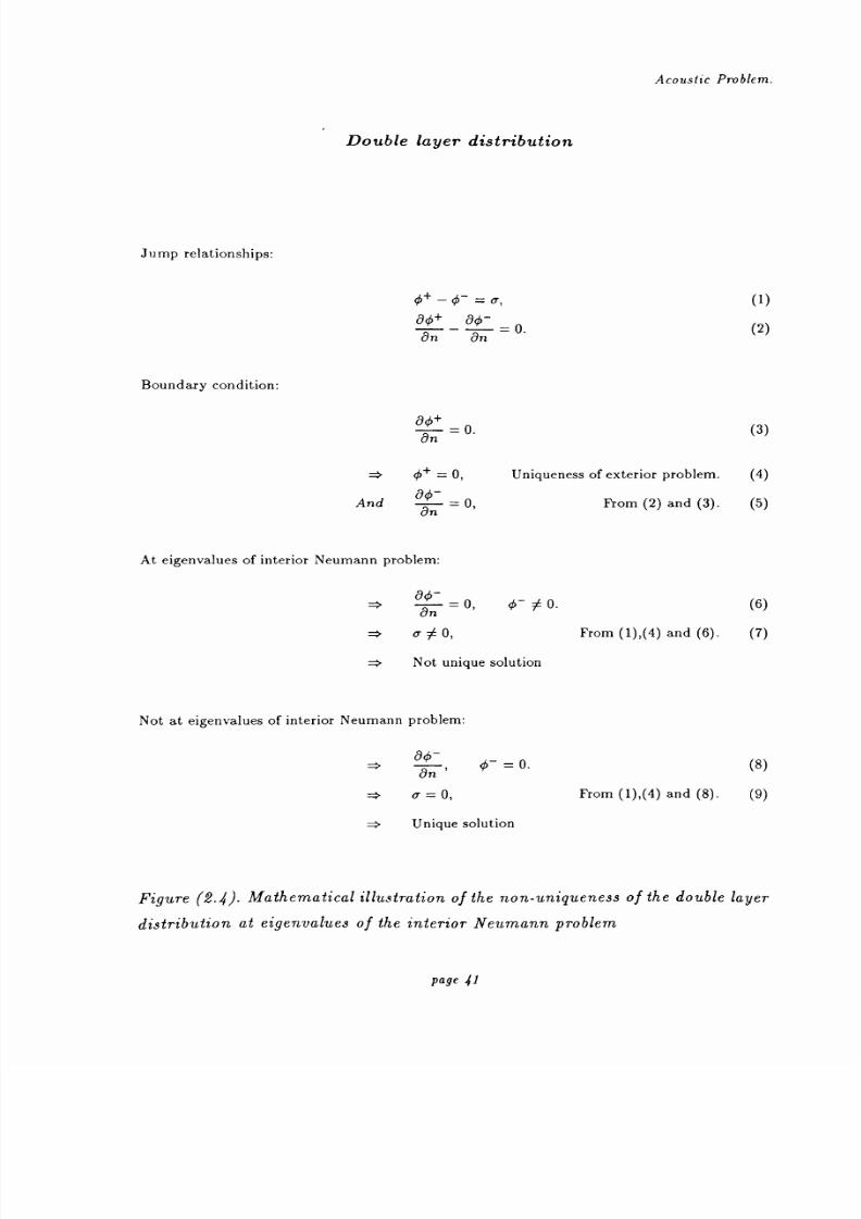
Acoustic Problem.
Double layer distribution
Jump relationships:
0+-0-=0-,
ao+ 00-
an an
(1)
(2)
Boundary condition:
ao+an =0
Z* 0+ = 0,
Andao-
= 0,
(3)
Uniqueness of exterior problem. (4)
From (2) and (3). (5)
At eigenvalues of interior Neumann problem:
as= o, 0-00.
0 o,
= Not unique solution
Not at eigenvalues of interior Neumann problem:
00
,_=0.ý
On
v=0,
Unique solution
(6)
From (1), (4) and (6). (7)
(8)
From (1), (4) and (8). (9)
Figure (2.4). Mathematical illustration of the non-uniqueness of the double layer
distribution at eigenvalues of the interior Neumann problem
Page 41

8/13/2019 Richard Jeans 1992 PhD Thesis
http://slidepdf.com/reader/full/richard-jeans-1992-phd-thesis 42/215
Acoustic Problem.
As the boundary layer formulation are related to the SHIE and the DSHIE, this hybrid
formulation is analogous to the Burton and Miller formulation described above.
2.5 Thin shell formulation
A prime motivation for this project was the analysis of thin shell acoustic problems. In this
work a thin shell is defined as a shell for which the through shell displacement field is assumed
to be constant. Acoustically this means that the normal derivative of pressure is the same on
both sides of the shell.
2.5.1 Boundary integral formulation
The geometry of the thin shell is illustrated in figure (2.5). On such a shell three closely
associated points may be defined. The points are p, p-, and p+, where p represents a point
midway through the thickness of the shell, p+ is a point on one surface, and p- is the corre-
sponding point on the other surface. The normal np is defined to be in the direction from p-
to p+. The Green's function and the normal derivative of Green's function at these points will
have the following simple relationships:
agS(g+anq
Gk(P, q4 ,
aGk(P,l)anq±
önq
= Gk (P, 4),
=OGk(P,
anq
E
np+
n
P-
n'
D
Figure (2.5). The thin shell geometry.
S+
S-
(2.5.1)
Page 42

8/13/2019 Richard Jeans 1992 PhD Thesis
http://slidepdf.com/reader/full/richard-jeans-1992-phd-thesis 43/215
4couslic Problfm.
Using these relationships, the SHIE formulation for the thin shell problem may be written as
O(P)= Oi(P)+ o(q+)aGk(P,g+)
SI+ aTZq+
+ (q)aGk(P,)an9-
_
o(q)Gk(P,
q+) dSq+9+
C)6(q)Gk(P,q+) dSq
.9-
(2.5.2)
By using the relationships in Eq. (2.5.1) and by setting gy(p) -- q(p+)-
0(p-), the SHIE
and DSHIE formulations for the thin shell become,
0(P) = Mk{41ý](P) + Q1(P),
a
n)= Nk[ý)(P) +
a¢a(P)
PEE, (2.5.3)
PEE. (2.5.4)
The surface domain S is now the surface of one side of the thin shell. Since S has been
redefined the domains D and E need also to be redefined. The domain D becomes the domain
whose interface with S contains the points p-, and E becomes the domain whose interface with
S contains the points p+. Both D and E are sub-domains of the exterior domain surrounding
S. Taking the limit of P to p in Eq. (2.5.3) and Eq. (2.5.4);
C(P)O+(P) + (1- c(P))O-(P) _ Mk[ ](P) + ci(P), PES, (2.5.5)
ao(P)=Nk[,l(P) +
ao (P)PES. (2.5.6)
an anp
2.5.2 Edge conditions
When considering thin shells which do not enclose an interior volume it is important to
consider the behaviour of the integral equations at the edge of this shell. It has been proposed
in previous work (WVarham [1988) that by taking the limit of P to p in from D and E, results
in two equations that give a condition on I. However if the limits are taken correctly then,
lim Mk[ ýD](P) _ -(P) =Mý[ý](P) + (1- c+(P))(O+(P) - -(P))p-.
P+
HM. vfk[I](P) _ 0-(P) =Mk[ i](P) -
(1- c_(P))(O+(P) -
p-
(2.5.7)
(2.5.8)
page 43

8/13/2019 Richard Jeans 1992 PhD Thesis
http://slidepdf.com/reader/full/richard-jeans-1992-phd-thesis 44/215
Acoustic Problem.
which leads to the identity,
ýý+ P) + c- p) - 1)ß P) = 0. 2.5.9)
This equation simply states the fact that c_ p) =1- c+ p) and gives no condition on D. A
more sophisticated argument is needed to define the edge conditions for the open plate problem.
When the thickness of the plate is taken to zero the edge around the plate becomes an
additional boundary. Consequently there needs to be a supplementary boundary condition
specified on this boundary. In his recent paper Martin [1991] discusses the behaviour of one-
dimensional hypersingular integral equations over finite intervals and this idea is discussed in
more detail. This edge boundary condition is arbitrary in the mathematical sense, but for this
case is governed by the original physical problem. Continuity of the pressure difference across
the plate means that Dmust be zero at the edge of the shell;
Dp) = 0, p on the edge. 2.5.10)
In past work eg. Pierce [1987]), this edge boundary condition has been satisfied by the
choice of appropriate fluid basis functions. In most numerical work for arbitrary thin plates e.g.
Terai [1981] and Warham [1988]) the edge boundary condition is essentially ignored since there
are no nodes on the edge of the plate. In the numerical work described in later chapters, the
presence of nodes on the edge of the plate means that this boundary condition must be imposed
upon the numerical formulation.
Page44

8/13/2019 Richard Jeans 1992 PhD Thesis
http://slidepdf.com/reader/full/richard-jeans-1992-phd-thesis 45/215
Collocation Mc fhod.
CHAPTER 3.
Collocation Method
3.1 Introduction
In this chapter a collocation method is described for the solution of radiation and scattering
problems for a submerged body of arbitrary geometry. A new way of numerically integrating
the hyper-singular kernels that occur in the boundary integral formulation is presented, and
the method is shown to be independent of the interpolation used for the fluid and geometrical
variables.Results for
a selection of scattering and radiation problems showthe
validity and
accuracy of the method.
The problem of uniqueness at critical wavenumbers is circumvented by implementing the
method of Burton and Miller, described in the previous chapter. High order quadrilateral
elements are used to interpolate for the acoustic and geometric variables.
3.2 Discretization
3.2.1 Interpolation
A number of connecting elements are defined on the surface domain. The nodal points
defined by these elements form the set of collocation points at which the boundary integral
equations are satisfied. Within the elements, the approximate fluid and geometric variables are
related to the element nodal values in terms of element shape functions. The nodal positions
of the element are defined in terms of the global Cartesian axes X, Y, Z), the local Cartesian
axes, x, y, z), define the normal and tangential planes at the Gauss integration points and the
curvilinear axes, ý, rl, ) define the element.
The approximations of global position and fluid variables are given in terms of the elemental
shape functions and element nodal values by,
mmm
X N1 ß,ý1)Xi, Y ý, ýI)= N1 ß,ýl)Yi,2 e,
ý1)_ Ný ý, ý1)z,. X3.2.1)
1=1 , =11=1
Nj ý, 77)01,90 ß, 77)
_ 11)and
3.2.2)
=1
an
1=1
In the definitions above, m. represents the number of nodes per element.
Page 45
8/13/2019 Richard Jeans 1992 PhD Thesis
http://slidepdf.com/reader/full/richard-jeans-1992-phd-thesis 46/215
Collocation.Method.
For this study 9-noded quadrilateral elements were used and the appropriate shape functions
are given by,
Ni = 4ýý - 1)ý1ýý]- 1),
N4 = 2ýý- 1)(1 - 7?),
N7 = 4ýýý- 1)i](7l + 1),
Na = zý1 -ý2)77(ýl - 1),
1'ß'5 (1 -0)(1
- q'),
N8=2(1_ý2)7J(1l+1),
X3 = 4ý(e + 1)i1(i7- 1),
N6= 2ý(ý+1)(1-112
N9 =4b+ 1)71(71+ 1),
Figure (3.1) shows the geometry for the 9-noded element. The approximation of a variable
within an element can be written in terms of the vector product,
0(ý,77)=
{Ne IT
loj
},(3.2.3)
where {Ne} is the vector of the element nodal shape functions defined at. (ý, i) and {QJ} is the
vector of nodal values of the variable 0 for element j.
3.2.2 Local and Curvilinear Axes
The curvilinear axes within the element are defined by,
where taking W=X,Y, and
2,
(gÄ( aY Z-e =ý -ex +a eY + a- eZ,
oÄ( aY aZ (3.2.4)e=
a, 7eX+- ä-eY, - (9ýeZ,
e( = ee x e,
aw _ y, 71) V1. (3.2.5)
The local axes vectors are derived from these curvilinear ones with the relationships,
ex = eý,
eZ = eý,
ey = e, x e,
(3.2.6)
where the hat notation for the vectors indicates normalization with respect to the global axes
system. By noting the orthogonality of the local axes, it is possible to write the Jacobian matrix
for the transformation between the local and curvilinear coordinate systems as,
Page 46

8/13/2019 Richard Jeans 1992 PhD Thesis
http://slidepdf.com/reader/full/richard-jeans-1992-phd-thesis 47/215
Collocation Method.
7
A5
12
8
9
ýy
x6
3
Z
Y
X
7
4
1
Figure 3.1). Geometry of the 9-noded isoparametric element.
Page 47
23

8/13/2019 Richard Jeans 1992 PhD Thesis
http://slidepdf.com/reader/full/richard-jeans-1992-phd-thesis 48/215
Collocation Method.
8dý
__iii
äý J21
0 aor
J-- dy (3.2.7)
With,
ax ax Oyii= =ex ee, Jai=ý=et e,,. J22==_ey
From these relationships the following Jacobian may be formed:
IJI= J11J22.
A vector that appears later in this chapter is defined by,
nq x Vqq.
this can be expanded in the local coordinate system as,
aoq x 7y 0=ax
ex -y ey.
eý. (3.2.8)
(3.2.9)
(3.2.10)
(3.2.11)
The relationship given in Eq. (3.2.7) allows this vector to be evaluated in terms of the curvilinear
axes thus enabling a numerical approximation.
3.3 Integration of Weak Singularity
There exist several numerical methods that enable a weak singularity to be integrated
within an element. For this study the inverse distance singularity scheme of Lachat and Watson
[1976] was used. In the collocation method a singularity will occur at the nodal points within an
element. In the Lachat and Watson scheme the singular element in the curvilinear axes system
is replaced by two, three, or four triangular elements with the singularity always at the same
corresponding vertex. These triangular elements are collapsed rectangular elements and the
number of subelements depends on whether the singularity is at a corner, mid-side, or center
node. When the Jacobian relating the integration over element and sub-element is calculated it
is found that the O(r-1) singularity is removed. Figure (3.2) shows the division of the 9-noded
element depending on the singular node.
page 48

8/13/2019 Richard Jeans 1992 PhD Thesis
http://slidepdf.com/reader/full/richard-jeans-1992-phd-thesis 49/215
Collocation Method.
1
2
Corner node
0
1
42
3
Center node
1
2
3
Mid-side node
Singularity
2
4c
3,4
Sub-element
Figure (3.2). Element sub-division for singular integration.
Page 49B133L
LONDIN.UNý/

8/13/2019 Richard Jeans 1992 PhD Thesis
http://slidepdf.com/reader/full/richard-jeans-1992-phd-thesis 50/215
Collocation Method.
The shape functions for the four-noded subelement, defined by the subelement axes ý,, and
r), are,
N13= 4(1 +ßs)(1 + als),
N3 =4(1
-ßs)(1
- ýIs)>
\ .4 =1 1-ßs)(1+7)s),
=4(1 +ý3)(1 -CJs)
The Jacobian is defined by,
IJ(ýs,ýs)I=äý äý
ýs qs
where,
o3ai18
as
ii=11
aSs
(3.3.1)
(3.3.2)
The superscript indicates the subelement nodal coordinate with respect to the 4,77axes. The
other terms in Eq. (3.3.1) are defined in a similar way.
Noting that ý3 = ý4 and r73 = q4, an expression for the subelement Jacobian can be
evaluated,
ýJ3(i3,0
I=-1
,q, + 1)-4,
(3.3.3)
where i is the number of the subelement and Ai is the area in the curvilinear space of that subele-
ment. The integration of a singular element can be transformed into an expression, removing
the singularity,
1subel
r(ý
1,
i1Jsdýsdiis (3.3.4)
Here r represents the distance between the singular node and the integration point in the
curvilinear space. In the modified integration scheme, the curvilinear points are interpolated
using the subelement shape functions defined above This transformation allows numerical
implementation using a simple Gauss integration.
3..4 Integral Operators
The object of any numerical method is to transform the governing equations into a system
of equations that is amenable to numerical solution. For a boundary element method this
page 50
8/13/2019 Richard Jeans 1992 PhD Thesis
http://slidepdf.com/reader/full/richard-jeans-1992-phd-thesis 51/215
Collocation Method.
involves approximating the integral equations, presented in Chapter 2, by discretized matrix
equations. This has to be done so that high order singularities and problems of non-uniqueness
of the numerical formulation are removed or circumvented. The integral operators that form
the components of the integral equations will be discussed individually.
3.4.1 £k Operator
This operator is defined by.
Gk [01(P)_
fGk(PQ)(Q)dSq.
(2.2.3)
The kernel of this integral operator contains singularities O(r-1) and there is no need to trans-
form this operator for numerical discretization. Using the element shape functions the,Ck
operator may be approximated by the following numerical expression,
ne
Gk[OI(P) _f Gk (P, q){Ne}T dS; {ý }. (3.4.1)
j =lS
Inthis equation, ne
isthe number of elements.
The integration isperformed numerically
inthe
curvilinear system using the method of Lachat and Watson described above. The surface field
point is interpolated using the element shape functions and the area element dSj is given by,
dS, -- IJ I<dq. (3.4.2)
When Eq. (3.4.1) is evaluated at each of the set of collocation points {Pt}, a system of
equations can be assembled. These equations can be written in matrix form in the following
way,
{, Ck[OI (Pi)l=
[Lk]{ }.
3.4.2 Mk Operator
This operator is defined by.
Mk[q5](P) =JaGäPýQ)q(Q)dsq.
Sq
(3.4.3)
(2.2.4)
page 51
8/13/2019 Richard Jeans 1992 PhD Thesis
http://slidepdf.com/reader/full/richard-jeans-1992-phd-thesis 52/215
Collocation alethod.
For this integral operator, the kernel contains singularities O(r-` ) and so a way is needed to
avoid the integration of high order singularities. The operator can be rewritten in the following
way,
[Mk -c(P)1]0= [Mk-Mol0+ [Mo-c(P)ll0.
Eq. (3.4.4) can be approximated in terms of the element shape functions,
n° aGk(P, q)_
3G0(ß.4)Mk ýýý(P) E Is, (
ön an{Ne}T dS; 10i }+
j=1 9 an,
iaý ÖG0(P, q)eT
anIN e dS; {0i }- c(p)O(P).
is
i
(3.4.4)
(3.4.5)
The second term on the right hand side of Eq. (3.4.5) contains singularities of O(r-2). This
singularity is ignored and Eq. (3.4.5) is integrated numerically using the modified numerical
integration technique. By taking the field point P to each of the collocation points a system of
equations can be assembled. These can be expressed in matrix form by,
{[Mk- C(P)1]I =
[Mk-
Cp]l01-
[Alk-_
lo]Lq} + [M0-
Cp]101. (3.4.6)
The diagonal matrix [Cp] is the value of c(P) evaluated at the collocation node points. Consider
the following definition of the last term in Eq. (3.4.6),
mil - cl
m21
[Mo-Cp]{O}=Mil
Mni
M12...
mli
m22 - c2 ... m2i
mat 772t; c;
mn2 mni
min Oi
M2n
02
ln2n Oi
mnn - Cn 0n
(3.4.7)
The O(r-2) singularities are distributed by the element shape functions to the diagonal elements
of this matrix. These matrix elements can be accurately defined by using a row sum procedure.
The definition of c(P) was given in Chapter 2 by,
j 0GoP, )ds.is
(3.2.13)
page 52
8/13/2019 Richard Jeans 1992 PhD Thesis
http://slidepdf.com/reader/full/richard-jeans-1992-phd-thesis 53/215
Collocation Method.
By using this relationship the diagonal elements of the matrix defined in Eq (3.1.7) are given
by,
mii - ci - -1 - mij.
j i
(3.4.8)
Therefore not only are the singular elements evaluated but c(p) is also implicitly evaluated.
The A4 operator may be numerically evaluated in a similar way. By redefining it as,
[Mk + c(P)Z] [Mk + Mo] - [Mo - c(P)Zj ß,
the operators in the numerical approximation are given by,
Tn, aGk (P, q) aGoýP, qý
e 7'
k[0](P)
-E On+
anIN } dSj { }-
? =1 ifp 9
n` r aGGO(P,Q)
eT
JS an{N } dSj {0j }- c(p)O(P).
j=1 q
This leads to the following matrix expression;
{ [MT + C(P)Z] 01 =[1ý1k + Cp]{0}
= [Mk + M0]{0} -[silo
-Cp]{q}
(3.4.9)
(3.4.10)
(3.4.11)
The first matrix on the right hand side of Eq. (3.4.11) contains singularities O(r-1) and the
O(r-2) singularities in the second matrix are evaluated using the row sum procedure described
above.
3.4.3 )/k Operator
This operator is defined by,
, i-ý[¢](P) =
a2Gk(P, Q)O(Q)dSq.
ön öns9P
(2.2.6)
It is this operator that, need the greatest amount of consideration when implementing a
numerical method since there are high order singularities that need integrating. Based on a
page 53

8/13/2019 Richard Jeans 1992 PhD Thesis
http://slidepdf.com/reader/full/richard-jeans-1992-phd-thesis 54/215
Collocation 11(thod.
proof shown by Maue [1949], it is possible to convert the expression in Eq. (2.2.6) into tangential
derivatives using the basic vector identity,
(np- Vq)(n9 - Vq) = (nn
-nq)(Vq 0)-
(nq x Vq) (np x Vq). (3.4.12)
By integrating by parts, the transformed expression for the Nk operator is given by,
Nk01(P)-J{(nP
. nq)k2Gk(P, q)O(q) -(nq xV
q0(q)) (nP x C9)Gk(P, q)] dSq+
S (3.4.13)is
n9 O9 x (q)(np x VgGk(P, q))] dSq.
The second term on the right hand side of Eq. (3.4.16) can be transformed by Stoke's theorem
into an integral around the edge of S. Therefore for closed surfaces it is equal to zero and can
be neglected. The transformed expression for the 111,Eoperator is finally given by,
Nk[01(P) =f [(np ' n9)k2Gk(P, 4)o(q) - (n9 X Vq (9)) . (np x Vq)Gk(P, q)] dSq. (3.4.14)s
The validity of this expression has been shown in greater detail by Stallybrass [1967] and Mitzner
[1966]. Eq. (2.2.6) can be rewritten in the following way,
Nk0=
[.Nk-
Vol 0+ %Voc (3.4.15)
The first operator on the right hand side contains terms of order O(r-1) and the second terms
of order O(r-2). Using the element shape functions Eq. (3.4.15) can be approximated by the
following expression,
Nk [01 (P)-J l(nP
j=1
nq)k2Gk(P, q){Ne}T _
(nq X Vq{Ne}T) (npx V9)(Gk(P, q) -Go(P, q))dS9 10i }-
ný/J
(nq x Vq{Ne}T) (np x V)Go(P. q)dSj { }.
1=1 J)
0i
(3.4.16)
page 54

8/13/2019 Richard Jeans 1992 PhD Thesis
http://slidepdf.com/reader/full/richard-jeans-1992-phd-thesis 55/215
Collocation.11ethod.
The O(-2) singularity in the second term of this expression is ignored for the time being and
Eq. (3.4.16) is evaluated at each collocation point to assemble the following matrix equation;
{-Nk[OJ(PP)} _ [, k]M _ [:Vk - .Vo){¢} + [_1 o]{yh}. (3.4.1 7)
This represents the matrix equation for the Nz operator, and no further modification is
made to integrate the singularity occurring in the [N0] term. It will be shown that there is
cancellation of the inaccuracies due to the numerical integration of these terms.
Consider thesingular
integrationover one element
for the A öoperator.
Thesingularity
is separated from the rest of the element by a disk segment of small radius e. The singular
integration over the element can be separated into a non singular integration over the element
minus the disk segment, Iý, and and a singular integration over the disk segment, Iý ;
Ij (nq XVq (4))-(np x V, GO(P,q))dS9 = I,
j,Ij,
.(3.4.18)
s,
The integration Iý is assumed to be accurate within the limits of the numerical integration
scheme. The inaccuracies for the element integration are assumed to be contained within the
integration Ij2. The small disk segment is assumed to be flat and the vector T is assumed to be
in the plane of the disk, perpendicular to the normal. The gradients within Eq. (3.4.18) can be
expressed as,
(nqx
Oq4(r, e))=
ö«r, B)(n9
X ), (3.4.19)3G0(r, B)
(np xV gGo(r,B)) = Or
(np x T),
The integration in Eq (3.4.18) can be rewritten as,
e Eä0(r, 6)2oGo(r, 0)Ij
-
In
8r ar rI JI drd9. (3.4.20)n
where the Jacobian IJI can be taken as constant. Within the disk segment it is assumed that 0
has a linear dependency on the global position vector and so in Eq (3.4.20) the variation of 0 is
independent from r and given by,
page 55

8/13/2019 Richard Jeans 1992 PhD Thesis
http://slidepdf.com/reader/full/richard-jeans-1992-phd-thesis 56/215
Collocation.1lfthod.
00)= pose
0Or
r-0
(OX
r=0sine y
r_0
(3.4.21)
Using this relationship Ij can be represented by,
Ii =Ii, +IB1jr.
(3.4.22)
For all elements j that contain the singularity there will be similar errors in Ir due to the
inadequate singular integration. However since the summation of the Ie terms is equal to zero
theseerrors cancel each other out.
Therefore it issafe
toevaluate the singular
terms inthe
[N. ]
matrix using the Lachat and Watson inverse distance singularity scheme.
In a recent paper by Wu, Seybert and Wan [1991] a very similar collocation method has
been described. This shows that Maue s equation needs C continuity at the collocation points
and to achieve this on CO continuous elements the collocation points are put inside the elements
to form an over determined set of equations. To achieve the integration of the Cauchy principal
value integral shown in Eq. (3.4.18) they use additional regularization.
This study uses a much more simple method. By integrating Eq. (3.4.18) for singular
elements directly it is recognized that there will be errors in the matrix approximation of the
X, operator. However this work has shown that there will be cancellation of these errors when
the acoustic problem is solved and so the sophisticated treatment of Eq (3.4.18) in the work by
Wu et al is unnecessary.
3.4.4 Matrix formulation
It is now possible to write the matrix approximation for the Burton and Miller boundary
integral equation, Eq. (2.4.4);
([Mk-
Cp] + a[Nk]) f01=
QLk} + a[Mk + cr]) {o}-foil -a
(90i
an ön
Eq. (3.4.23)represents a matrix equation of
the form,
[H]x =
(3.4.23)
(3.4.24)
page 56

8/13/2019 Richard Jeans 1992 PhD Thesis
http://slidepdf.com/reader/full/richard-jeans-1992-phd-thesis 57/215
Collocation Method.
where the matrix [H], is full, complex and non-symnmetric. In the past considerable effort
has been made to symmetrize this matrix equation (Mathews [1986]). For this study this non
symmetric equation set was solved directly using a standard LU-factorization technique followed
by forward and backward substitution. The imaginary coupling constant a takes the value i/k,
since this has been shown by previous researchers (Burton and Miller [1971]) to be the optimum
value. For the numerical integration 3x3 Gauss integration was used for both the non singular
elements and for the Lachat and Watson subelements.
3.4.5 Exterior pressure distribution
The exterior pressure distribution is given by,
Os P) _ Mk[0](P) - £k[01(P). PEE. (3.4.25)
This expression can be approximated numerically by using the element shape functions,
(P)_
öGk(P, q) {Ne}dS {( )- Gk (P, q){Ne}dSai
(3.4.26)
=1
fSa9(is
a=1 i=1 I
Since the field point P is exterior to the boundary surface there is no singular kernel in this
expression that needs special consideration.
For the far field pressure distribution this numerical expression can be further simplified.
By considering the geometry shown in figure (3.3) it is possible to write,
Off(P) _
eikRný /ý a
kiý)f
4ýRiknq - ReikR. 9{Ne}dS {¢ý }-J ei
q{: ý e}dS anJs S
(3.4.27)
where R represents the far-field field point vector and q represents the boundary surface point.
In vector form this expression can be written as
o3- lMkf J
{0}-
{L k }
an(3.4.28)
page 57

8/13/2019 Richard Jeans 1992 PhD Thesis
http://slidepdf.com/reader/full/richard-jeans-1992-phd-thesis 58/215
Collocation Method.
Figure (3.3) Geometry for evaluating the far field pressure distribution.
3.5 The computer code
The numerical implementation of the collocation method was coded in FORTRAN predom-
inantly on an IBM RS6000 machine in a UNIX environment. The code was written to primarily
evaluate the numerical method presented above and it was found that in core memory space
was large enough to run problems of a large enough size to demonstrate accuracy for a number
of simple geometries.
Use was made of structural geometry in order to reduce the problem size considerably. This
was done by specifying a degree of rotational symmetry about the global Z axis and in most
cases only one axisyinmetric quarter of the acoustic structure is actually discretized.
3.6 Numerical results
3.6.1 Radiation fron submerged spheres
One axisymmetric quarter of a sphere with radius a is discretized into a number of elements
of equal area. Figure (3.4) shows the different mesh geometries for the spherical problem, A
surface velocity with a Legendre distribution is specified on the sphere,
ao aooan an P(cos9).
The resulting normalized acoustic impedance, Z, is calculated,
(3.6.1)
page 58

8/13/2019 Richard Jeans 1992 PhD Thesis
http://slidepdf.com/reader/full/richard-jeans-1992-phd-thesis 59/215
Collocation fcihod.
Z-ko/0'0. (3.6.2)
and further normalized with respect to P, to form the normalized modal acoustic impedance.
The results for various discretizations and modes are plotted with respect to wavenuinber
in figures (3.5-8). These results are compared to the analytical solution (Junger and Feit [1986])
and show high accuracy and good convergence.
The effectiveness of the of the Burton and 1-filler formulation in removing the problem of
non-uniqueness at critical frequencies is shown in figures (3.9-10). The error in the normalized
modal impedance is plotted at the internal acoustic eigenvalues for the interior spherical problem,
for ka less than 10. These eigen-frequencies can be calculated analytically. The error plots show
quite clearly the high errors for the SHIE and DSHIE formulations around the appropriate
critical frequencies of the interior problem. These plots also show that with the Burton and
Miller formulation, the error in modal impedance for these modes is less than 0.1 for n=0,
less than 1 for n=1 and n=2 and less than 5 for n=3.
3.6.2 Acoustic scattering from a submerged sphere
Figure (3.11) shows the convergence of the backscattered far-field form function for scat-
tering of a plane wave by a rigid sphere compared to an analytical solution. The incident wave
is defined by,
Oi = eikz (3.6.3)
and the backscattered far-field form function is given by,
2R 10,=
aa(3-6.4)
This plot shows good convergence to the analytical solution and the low and high frequency
characteristics of plane wave scattering. At low frequency the form-function depends on k2 as
Raleigh scattering is predominant. In this frequency regime the acoustic wavelength is large
compared to the scatterer and the form-function depends only on the volume of the sphere. At
higher frequencies the form-function converges to the Kirchoff limit. In this frequency regime
it is the specular reflections from the illuminated surfaces that dominate and for the sphere the
page 59

8/13/2019 Richard Jeans 1992 PhD Thesis
http://slidepdf.com/reader/full/richard-jeans-1992-phd-thesis 60/215
Collocation Ifcthod.
Kirchoff approximation predicts a frequency independent form-function, dependent on the area
of the illuminated surface. This frequency plot also shows the characteristic oscillations due to
the interference of Franz waves.
Figures (3.12-13) show the scattering distribution in the Y-Z plane for various frequencies.
The axis magnitudes for these plots is the Y-Z components of the far-field pressure amplitude
with unit magnitude incident plane wave. Again the numerical results are compared to an
analytical solution.
Figure (3.14) shows the amplitude of the surface pressure in the Y-Z plane for the
same unit amplitude incident plane wave, at two frequencies for different discretizations. The
plotted points in this figure correspond to the nodal points on the surface mesh. These points are
compared to the analytical solution. It is worth noting that for 24 elements the far-field accuracy
seems to be greater than the surface accuracy. This indicates a degree of error `smoothing when
calculating the far-field quantities.
3.6.3 Acoustic scattering from a submerged spheroid
The figures (3.15-16) show the far-field scattering distributions for oblate and prolate
spheroids. One axisymmetric quarter of the spheroid is discretized and the plane-wave is taken
to be incident end on to preserve the axisyinmetry of the problem.
In the absence of any sophisticated meshing algorithm, the mesh for the spheroids was
calculated by simply scaling the spherical mesh in the X, Y, Z directions. The comparison to
the numerical results was provided by the program written by S.W. Wu, for his PhD project
[1990]. This program was written to solve for purely axisymmetric acoustic problems using high
order line-elements. The program was run using 20 such elements and the assumption made that
this represented a converged solution. There seems to be a high degree of accordance between
the results. These test cases show the efficiency of the model for geometries other than the
simple spherical problem described above.
3.6.4 Acoustic scattering from a submerged finite cylinder
The last set of numerical results concerns the far-field scattering distribution from a finite
cylinder of length L and radius a. The mesh geometries for this problem are shown in Figure
(3.17). Again only one axisynunetric quarter of the cylinder is discretized and the plane wave is
incident. along the Z axis. The numerical results are compared to the results of S.W. Wu using
44 axi-syrrunetricline elements.
page 60

8/13/2019 Richard Jeans 1992 PhD Thesis
http://slidepdf.com/reader/full/richard-jeans-1992-phd-thesis 61/215
Collocation.fethod.
Figure 3.18) shows the far field scattering results for a cylinder with length 4a and 8a.
Both plots in the figure show good agreement with the results of S.W. \Vu. Figure 3.19) shows
the convergence of the scattering distribution from the L=8.0 cylinder. This figure shows the
importance of a high density of elements around the surface discontinuities, as is the case for
the 104 element mesh.
page 61
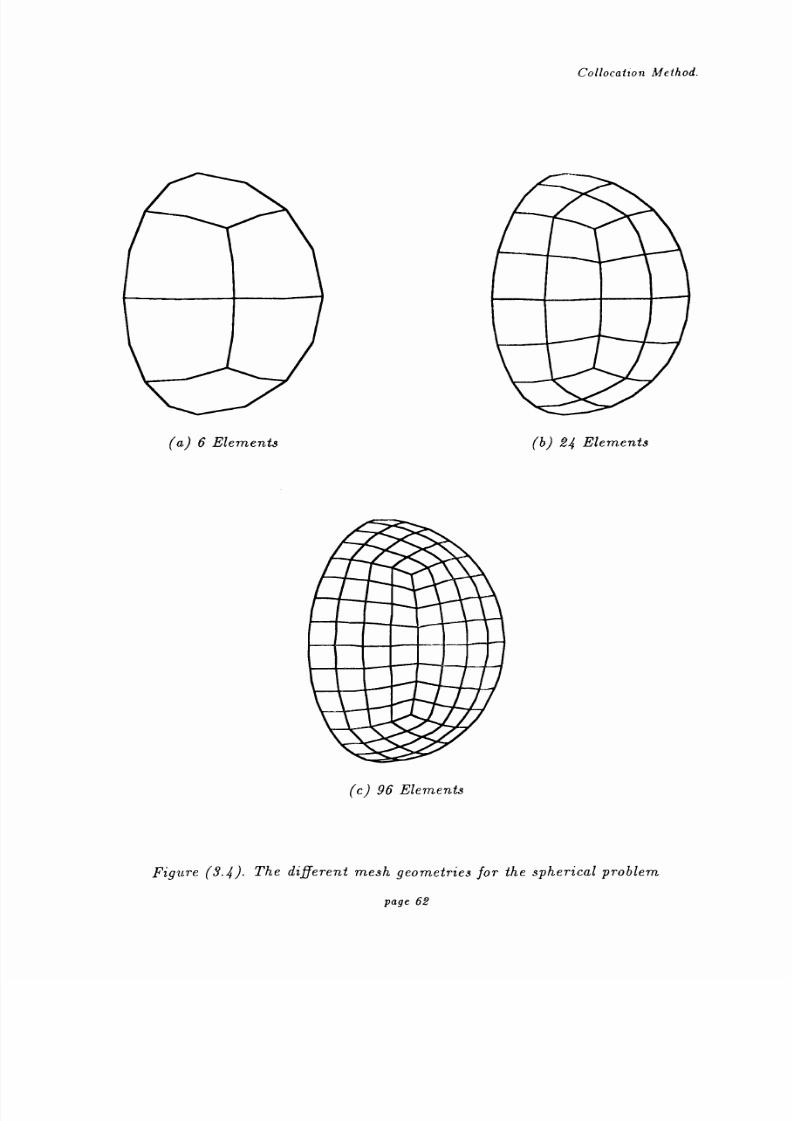
8/13/2019 Richard Jeans 1992 PhD Thesis
http://slidepdf.com/reader/full/richard-jeans-1992-phd-thesis 62/215
Collocation Method.
a) 6 Elements
c) 96 Elements
b) 24 Elements
Figure 3.4). The different mesh geometries for the spherical problem
page 62

8/13/2019 Richard Jeans 1992 PhD Thesis
http://slidepdf.com/reader/full/richard-jeans-1992-phd-thesis 63/215
Collocation Method.
1.5
Z
1.0
n=O
0.5
0.0
-0.5
-1.0`0
1.5
Z
1.0
0.5
0.0
-0.5
1n
246g ka 10
1 .V
02468 ka 10
Analytical Real . Imaginary A.
Figure 3.5). Normalized modal impedance for the rigid sphere, modes 0 and 1.
One axisymmetric quarter of the sphere, radius a, is discretized into 6 elements.
page 63
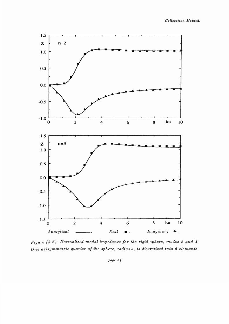
8/13/2019 Richard Jeans 1992 PhD Thesis
http://slidepdf.com/reader/full/richard-jeans-1992-phd-thesis 64/215
Collocation Method.
1.5
Z
1.0
n=2
0.5
0.0
-0.5
-1.002
1.5
Z n=3
1.0
0.5
0.0
-0.5
-1.0
-1.502468 ka 10
Analytical Real . Imaginary
Figure 3.6). Normalized modal impedance for the rigid sphere, modes 2 and 3.
One axisymmetric quarter of the sphere, radius a, is discretized into 6 elements.
4 6 g ka 10
page 64
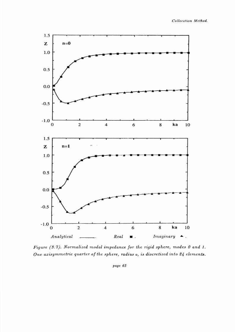
8/13/2019 Richard Jeans 1992 PhD Thesis
http://slidepdf.com/reader/full/richard-jeans-1992-phd-thesis 65/215
Collocation Method.
1.5
Z
1.0
n-0
0.5
0.0
-0.5
-1.00
1.5
Z
1.0
0.5
0.0
-0.5
1
2 4 6 g ka 10
n=1
02468 ka 10
Analytical Real . Imaginary &.
Figure (3.7). Normalized modal impedance for the rigid sphere, modes 0 and 1.
One axisymmetric quarter of the sphere, radius a, is discretized into 24 elements.
page 65
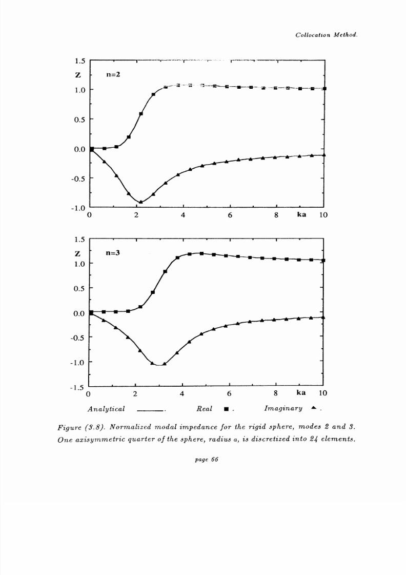
8/13/2019 Richard Jeans 1992 PhD Thesis
http://slidepdf.com/reader/full/richard-jeans-1992-phd-thesis 66/215
Collocation Method.
1.5
Z
1.0
0.5
0.0
-0.5
1A
n=2
-I. V
0246
1.5
Z n=31.0
0.5
0.0
-0.5
-1.0
-1.502468 ka 10
Analytical Real . Imaginary A.
Figure 3.8). Normalized modal impedance for the rigid sphere, modes 2 and 3.
One axisymmetric quarter of the sphere, radius a, is discretized into 24 elements.
g ka 10
page 66

8/13/2019 Richard Jeans 1992 PhD Thesis
http://slidepdf.com/reader/full/richard-jeans-1992-phd-thesis 67/215
Collocation Method.
1040 0
0103 n=0
LOL
102ee
101eo
e0100
000ee
dý 0 A
10-1 epe aoA
sse0
o0a®e e ®e G
0
10 -2 00
10-3
10-402468 ka 10
10400
103 n=1LO
L 102eeA
101 0
o AAA
100 eeA000A, & A 8
es010 -1 00 oQs:
Oam O ta NW MI
102 -
'Do
103
10-402468 ka 10
Coupled . SHIE o. DHSIE '& .
Figure (3.9). Normalized error of modal impedance for the rigid sphere, modes
0 and 1. One axisymmetric quarter of the sphere, radius a, is discretized into
24 elements.
page 67

8/13/2019 Richard Jeans 1992 PhD Thesis
http://slidepdf.com/reader/full/richard-jeans-1992-phd-thesis 68/215
Collocation Method.
104
103
OV
L 102
101
10°
10-1
10-2
10-3
, n-4
n=2
A
A
0
A
0e0°°00
Ao
g °o °o
00 0° ® ®
oo000
0
sIV
02468 ka 10
104
103 n=3LA00`
10 2es
101Ls e
000 AS 00ae10
0CPA
°0 o49A
10 -10o0 Le
00
00 MEN
o
10 -2 00
103
10-402468 ka 10
Coupled . SHIE o. DHSIE.
Figure (8.10). Normalized error of modal impedance for the rigid sphere, modes
2 and 3. One axisymmetric quarter of the sphere, radius a, is discretized into
24 elements.
page 68

8/13/2019 Richard Jeans 1992 PhD Thesis
http://slidepdf.com/reader/full/richard-jeans-1992-phd-thesis 69/215
Collocation Method.
o
0
0
0
0
0
0
0
0
0
0
kn
Itt
M
N
. --4
O 00 ýO ýt NO 00 N
ri - r-+ .-OOOOO
uo Jz)un, uuao3
6 elements 0.24 elements .
Figure (4.11). Plane wave backscattered form function for therigid sphere.
One axisymmetric quarter of the sphere, radius a, is discretized into 6 and 24
elements.
page 69

8/13/2019 Richard Jeans 1992 PhD Thesis
http://slidepdf.com/reader/full/richard-jeans-1992-phd-thesis 70/215
Collocation Method.
ka=0.1
0.015
0.010
0.005
0.000
-0.005
-0.010
-0.0154--
-0.020 -0.015 -0.010
ka=1
0.80.6
0.4
0.2
0.0
-0.2
-0.4-0.6
-0.8
-1.0
-0.005 0.000 0.005
Analytical Numerical
Figure S. 12). Far field form function distribution for scattering of an incident
plane wave by a rigid sphere. The plane wave is incidentfrom left
to right.One
axisyinmetric quarter of the sphere, radius a, is discretized into 24 elements and
the distribution is calculated at ka = 0.1 and 1.0
page 70
-0.8 -0.6 -0.4 -0.20.0 0.2 0.4
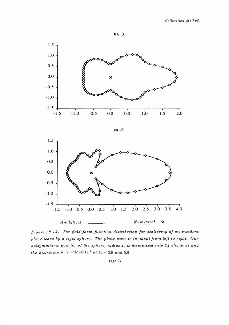
8/13/2019 Richard Jeans 1992 PhD Thesis
http://slidepdf.com/reader/full/richard-jeans-1992-phd-thesis 71/215
Collocation Method.
ka=3
1.5
1.0
0.5
0.0
-0.5
-1.0
-1.5
-1.5
ka=5
1.5
1.0
0.5
0.0 X
-0.5
-1.0
-1.5
-1.5 -1.0 -0.5 0.0 0.5 1.0 1.5 2.0 2.5 3.0 3.5 4.0
Analytical Numerical O.
Figure 3.13). Far field form function distribution for scattering of an incident
plane wave by a rigid sphere. The plane wave is incident from left to right. One
axisymmetric quarter of the sphere, radius a, is discretized into 24 elements and
the distribution is calculated at ka = 3.0 and 5.0
page 71
-1.0 -0.5 0.0 0.5 1.0 1.5 2.0

8/13/2019 Richard Jeans 1992 PhD Thesis
http://slidepdf.com/reader/full/richard-jeans-1992-phd-thesis 72/215
Collocation Method.
ka=3
1.5
1
0.5
0
-0.5
-1
-1.5
-2
2
1.5
1
0.5
0
-0.5
-1
-1.5
-2
-2.5
-1.5 -1 -0.5 0 0.5 1 1.5
ka=5
-2 -1.5 -1 -0.50 0.5 1 1.5
Analytical 24 Elements 13.96 Elements
Figure 3.14). Amplitude of surface pressure for plane wave scattering by a rigid
sphere. The plane wave is incident from left to right. One axisymmetric quarter
of the sphere, radius a, is discretized into 6 and 24 elements and the distribution
is calculated at ka = 3.0 and 5.0
page 72

8/13/2019 Richard Jeans 1992 PhD Thesis
http://slidepdf.com/reader/full/richard-jeans-1992-phd-thesis 73/215
Collocation Method.
a=1.0 b=0.2k=1.0
0.20
0.10
0.00
-0.10
-0.20 .ý-
-0.40
.1
-0.20 0.00
a=1.0 b=0.2 k=3.0
0.8
0.6
0.4
0.2
0.0
-0.2
-0.4
-0.6
-0.8_1.8
0.20 0.40
-1.4 -1.0 -0.6 -0.20.2 0.6 1.0 1.4 1.8
S. W. Wu Numerical O.
Figure 8.15. Farfield pressure distribution for scattering of an incident plane
wave by a rigid oblate spheroid. The plane wave is incident from lefto right.
One axisymmetric quarter of the spheroid is discretized into 96 elements and
the distribution is calculated at k=1.0 and k=3.0. The results of S. W. Wu were
calculated using 20 axisymmetric line elements.
page 73

8/13/2019 Richard Jeans 1992 PhD Thesis
http://slidepdf.com/reader/full/richard-jeans-1992-phd-thesis 74/215
Collocation Method.
a=0.2 b=1.0 k=1.0
0.02
0.01
0.00
-0.01
-0.02
-0.02 -0.01 0.00 0.01
a=0.2b=1.0k=3.0
0.05
0.03
0.01
-0.01
-0.03
-0.05 -
-0.05
S. W. Wu Numerical
Figure 3.16). Farfield pressure distribution for scattering of an incident plane
wave by a rigid prolate spheroid. The plane wave is incident from left to right.
One axisymmetric quarter of the spheroid is discretized into 96 elements and
the distribution is calculated at k=1.0 and k=3.0. The results of S. W. Wu were
calculated using 20 axisymmetric line elements.
Page 74
-0.03 -0.010.01 0.03 0.05

8/13/2019 Richard Jeans 1992 PhD Thesis
http://slidepdf.com/reader/full/richard-jeans-1992-phd-thesis 75/215
Collocation Method.
a) 72 Elements
b) 88 Elements
c) 104 Elements
Figure 3.17. The differentmesh geometries for the cylinder problem
page 75

8/13/2019 Richard Jeans 1992 PhD Thesis
http://slidepdf.com/reader/full/richard-jeans-1992-phd-thesis 76/215
Collocation Method.
a=1.0 L=4.0 k=1.0
0.6
0.4
0.2
0
-0.2
-0.4
-0.6
-0.7 -0.5 -0.3 -0.1 0.1 0.3
a=1.0L=8.0 k=1.0
0.6
0.4
0.2
0
-0.2
-0.4
-0.6
-0.6 -0.4 -0.20 0.2 0.4
0.5
0.6
S. W. Wu Numerical O.
Figure 3.18). Farfield pressure distribution for scattering of an incident plane
wave by a rigid cylinder. The plane wave is incident from left to right. The
distribution is calculated at k=1.0 for L=4.0 and L=8.0. One axisymmetric
quarter of the cylinder is discretized into 72 elements for L=4.0 and 104 elements
for L=8.0. The results of S. W. Wu were calculated using 44 axisymmetric line
elements.
page 76

8/13/2019 Richard Jeans 1992 PhD Thesis
http://slidepdf.com/reader/full/richard-jeans-1992-phd-thesis 77/215
Collocation Method.
\oö
Ö
0
0
II
0
ea
i .`
ýi
1
NO
0
N9
9
Ö
S. W. Wu.72 Elements f
.88 Elements 13.104 Elements .
Figure 8.19). Convergence
ofthe farfield
scatteringdistribution from
the cylin-der, L=8.0, a=1.0, at a wave number of k=1.0.
yý4
1N
.w.
page 77
ýt NO C14 lqt ýcÖCCÖÖÖ
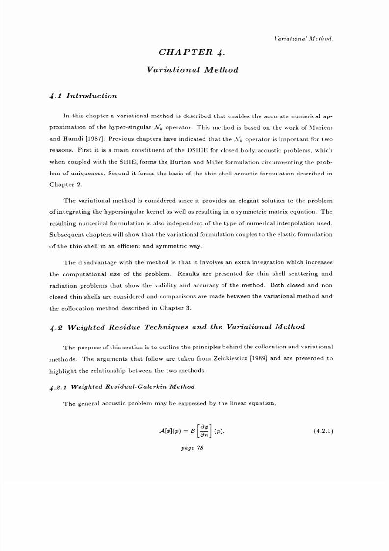
8/13/2019 Richard Jeans 1992 PhD Thesis
http://slidepdf.com/reader/full/richard-jeans-1992-phd-thesis 78/215
I ariaftonal.110hod.
CHAPTER
Variational Method
4.1 Introduction
In this chapter a variational method is described that enables the accurate numerical ap-
proximation of the hyper-singular Yk operator. This method is based on the work of Mariem
and Hamdi [1987]. Previous chapters have indicated that the.A operator is important for two
reasons. First it is a main constituent of the DSHIE for closed body acoustic problems, which
when coupled with the SHIE, forms the Burton and Miller formulation circumventing the prob-
lem of uniqueness. Second it forms the basis of the thin shell acoustic formulation described in
Chapter 2.
The variational method is considered since it provides an elegant solution to the problem
of integrating the hypersingular kernel as well as resulting in a symmetric matrix equation. The
resulting numerical formulation is also independent of the type of numerical interpolation used.
Subsequent chapters will show that the variational formulation couples to the elastic formulation
of the thin shell in an efficient and symmetric way.
The disadvantage with the method is that it involves an extra integration which increases
the computational size of the problem. Results are presented for thin shell scattering and
radiation problems that show the validity and accuracy of the method. Both closed and non
closed thin shells are considered and comparisons are made between the variational method and
the collocation method described in Chapter 3.
4.2 Weighted Residue Techniques and the Variational Method
The purpose of this section is to outline the principles behind the collocation and variational
methods. The arguments that follow are taken from Zeinkiewicz [1989] and are presented to
highlight the relationship between the two methods.
4.2.1 Weighted Residual-Galerkin Method
Thegeneral acoustic problem may
be
expressed
by the linear equation,
A[O] p) =8ý P) 4.2.1)
page 78

8/13/2019 Richard Jeans 1992 PhD Thesis
http://slidepdf.com/reader/full/richard-jeans-1992-phd-thesis 79/215
Variational .11cthod.
Eq. (4.2.1) n-iust be satisfied at every point, p, on some surface domain, S. It follows therefore
that;
isu.,p)A[¢](P)dSp =J u'(P)B ön
(P)dSp,is
(4.2.2)
where w is a weighting function and Eq. (4.2.2) must be satisfied for all w. The fluid variables
may be approximated in terms of the global shape functions,
{N9}T {0},a0 : 1, -g IT fan
(4.2.3)
If the approximated values of the fluid variables are inserted into Eq. (4.2.2) then it is clearly
impossible for this expression to be satisfied for all uw. nstead an approximation is made and u'
is replaced by a finite set of weighting functions so that,
w= wj, j=1 to n. (4.2.4)
Eq. (4.2.2) will now yield a set of n simultaneous equations given by,
fw(P)A[{'ßr9}T
}](p)dS= J w(P)13 {N}T'91]
(P)dS. (4.2.5)s
This equation represents an integral of error residuals and clearly the equation set generated
depends on the set of weighting functions that are chosen.
If the weighting functions are chosen so that,
wi = b(P- Pj), (4.2.6)
where pj is the set of nodal points then Eq. (4.2.5) will correspond to the collocation method
described in Chapter 3. If however the weighting functions are chosen so that,
Wj _ :ý'J
,
then Eq. (4.2.5) is the Galerkin weighted residual method.
(4.2.7)
page 79

8/13/2019 Richard Jeans 1992 PhD Thesis
http://slidepdf.com/reader/full/richard-jeans-1992-phd-thesis 80/215
Variational.f0hod.
4.2.2 Variational Method
For the variational method some scalar functional is generated using some a priori guess
as to the physical nature of the problem. For some physical problems this scalar functional
may correspond to the potential energy or the energy dissipation of the system. The solution
of the problem is achieved by minimizing this functional with respect to the unknown variable.
Consider the BEM formulation for the thin shell acoustic problem defined in Chapter 2,
a4 P)
_ Alk [ýDl P)- 4.2.8)an
The appropriate functional is defined by,
n=I ý3O- 2ýA1
[<D]p) dSp. 4.2.9)9n
The minimization of this functional gives the variational formulation of the problem. Due to
the symmetry of the J1/k operator, the stationary value problem can be evaluated in a straight
forward manner,
bII =I b a P)-
b DA-k[ DIP) dSp = 0. 4.2.10)
It can be seen that this expression is identical to the Galerkin formulation of the thin shell
problem. In general if the governing integral operator is self adjoint then the variational and
Galerkin formulations will be identical. The whole subject of variational methods is discussed
in great detail in the book by Morse and Feshbach [1953].
4.3 Variational Boundary Integral Formulation
The full boundary integral equation for the thin shell problem is defined by,
ao p)
_ A,k[ýJ P)
as P)P
2.5.6)
where 1 is the pressure difference across the shell. Following the method shown in Chapter 3
the Nk operator can be transformed into tangential derivatives;
page 80
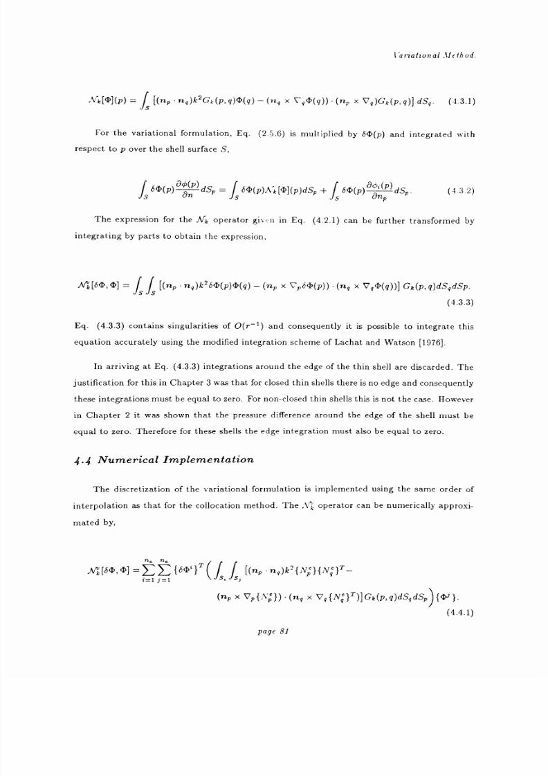
8/13/2019 Richard Jeans 1992 PhD Thesis
http://slidepdf.com/reader/full/richard-jeans-1992-phd-thesis 81/215
Variational If0hod.
[(tp *f9)k2Gk(P, q)4(q) -
(n9 X Vq (q))-
(nP x Vq)C'k(P,q)] dSq. (4.3.1)
For the variational formulation, Eq. (2.5.6) is multiplied by 6D(p) and integrated with
respect to p over the shell surface S,
Ibý(P)
aanP)dsp =
Ibý(p)i1
k[<D](p)dSp+ &D(p)aý (P)
dSp. (4-3.2)s
is
p
The expression for the Alk operator given in Eq. (4.2.1) can be further transformed by
integrating by parts to obtain the expression,
All [6,ý] =ff
[(np' nv)k26D(P)(D(4') -
(np x GPb(D(P)) ' (nq x Vq(D(q))] Gk(p, q)dSgdSp.ss
(4.3.3)
Eq. (4.3.3) contains singularities of O(r-1) and consequently it is possible to integrate this
equation accurately using the modified integration scheme of Lachat and Watson [1976].
In arriving at Eq. (4.3.3) integrations around the edge of the thin shell are discarded. The
justification for this in Chapter 3 was that for closed thin shells there is no edge and consequently
these integrations must be equal to zero. For non-closed thin shells this is not the case. However
in Chapter 2 it was shown that the pressure difference around the edge of the shell must be
equal to zero. Therefore for these shells the edge integration must also be equal to zero.
4.4 Numerical Implementation
The discretization of the variational formulation is implemented using the same order of
interpolation as that for the collocation method. The Vk. operator can be numerically approxi-
mated by,
ýe ne
E {bit T l [(npnq)k`2{N
}{Ng }T
_i=1 j-1 I>
(nP X OPlApj)-(n9 X Vq{NgIT)]Gk(P,9)dSqdSp W}.
(4.4.1)
page 81

8/13/2019 Richard Jeans 1992 PhD Thesis
http://slidepdf.com/reader/full/richard-jeans-1992-phd-thesis 82/215
Variational Alethod.
In Eq. 4.4.1) the gradient of the shape function is expressed in terms of the local coordinate
axis system. In order to evaluate these gradients it is necessary to use the relationship shown
in Eq 3.2.11). The Jacobian matrix for the system, defined in Eq. 3.2.7), then enables the
gradient to be expressed in derivatives of the curvilinear system.
For the integration in Eq. 4.4.1), the point p ranges over Si and the point q ranges over Sj.
The integration with respect to p is performed using simple Gauss integration. The singularities
in the above numerical approximation will occur at these Gauss integration points when i=j.
It is these auto-influence elements that need to be integrated using the Lachat and Watson
singular integration scheme. For the integration with respect to q, the element, will be divided
as shownin figure 4.1)
Singularity at Gausspoint
Figure 4.1). Subelement division.
The expression in Eq. 4.4.1) can be assembled into a matrix formulation of the variational
problem,
[N{}
-A
a0
-190`
= 0. 4.4.2).älß an
where the matrix [A] represents the numerical approximation,
ne
r
{Ne}{Ne}TdS 4.4.3)o}T [A]{O} =E {b4ti}T
Isi
j=1
In practice this banded symmetric matrix may be further approximated by the diagonal matrix,
page 82
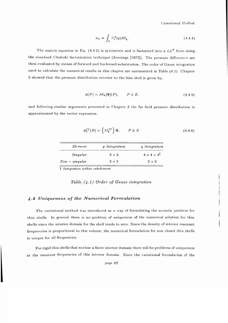
8/13/2019 Richard Jeans 1992 PhD Thesis
http://slidepdf.com/reader/full/richard-jeans-1992-phd-thesis 83/215
Variational Method.
aii =i' ,(4) dSq.
S
(4.4.4)
The matrix equation in Eq. (4.4.2) is symmetric and is factorized into a LLT form using
the standard Choleski factorization technique (Jennings [1977)). The pressure differences are
then evaluated by means of forward and backward substitution. The order of Gauss integration
used to calculate the numerical results in this chapter are summarized in Table (4.1). Chapter
2 showed that the pressure distribution exterior to the thin shell is given by,
0 (P) _ (4.4.5)
and following similar arguments presented in Chapter 3 the far field pressure distribution is
approximated by the vector expression,
Osf(R) _{111kf}
ý, PEE.
Element p Integration q Integration
Singular 3x3
Non - singular 2x2
j Integration within subelement
4x4x4t
2x2
Table (4.1) Order of Gauss integration
4.5 Uniqueness of the Numerical Formulation
(4.4.6)
The variational method was introduced as a way of formulating the acoustic problem for
thin shells. In general there is no problem of uniqueness of the numerical solution for thin
shells since the interior domain for the shell tends to zero. Since the density of interior resonant
frequencies is proportional to this volume, the numerical formulation for non closed thin shells
is unique for all frequencies.
For rigid thin shells that enclose a finite interior domain there will be problems of uniqueness
at the resonant frequencies of this interior domain. Since the variational formulation of the
page 83
8/13/2019 Richard Jeans 1992 PhD Thesis
http://slidepdf.com/reader/full/richard-jeans-1992-phd-thesis 84/215
Variational Method.
problem is equivalent to the double boundary layer formulation detailed in Chapter 2, the
numerical solution will become ill-conditioned at eigenvalues of the interior Neumann problem.
Althougha
hybrid boundary layer formulationovercomes these problems of uniqueness, the
resulting boundary layer potential is no longer equivalent to the pressure difference across the
shell. The reason for this is that a natural variational formulation of the hybrid problem does
not exist, and the corresponding Galerkin formulation is non-symmetric.
In this chapter no effort is made to circumvent the problems of uniqueness that arise for
rigid closed thin shells. However Chapter 6 will demonstrate that for the elastic, closed thin
shells, the formulation is unique at all frequencies.
4.6 Edge Boundary Conditions
In Chapter 2 it was shown that for non closed thin shells it is necessary to enforce an
edge boundary condition. The physical reality of this is that the pressure difference across the
shell must be zero at the edges. Since this boundary condition is not implicit in the collocation
or variational numerical approximation of the .k operator, then it must be imposed on the
resulting matrix equation set.This
matrix equation set canbe
representedby,
[H]{ýD} = {y}, (4.6.1)
where [H] is the matrix approximation of the collocation or variational formulation and {y} is
the appropriate right hand side of this matrix equation;
[A] {an -
0 } Variational,(4.6.2)y} =
a0_
Collocation.an an
}
Defining { EJ and {(DI} as those elements of the vector that correspond to edge or interior
nodes, Eq. (4.6.1) can be rewritten as,
HII HIE (b I yI
YEEI HEE
41>E
(4.6.3)
The interior pressure differences can now be written in terms of the known edge pressure
differences and the known vector {yl},
page 84

8/13/2019 Richard Jeans 1992 PhD Thesis
http://slidepdf.com/reader/full/richard-jeans-1992-phd-thesis 85/215
Variational.fethod.
[HIf]Oýj}-
{y }-
[HIE]{(ýE}. (4.6.4)
If (D is equal to zero on the edge of the plate, this equation reduces to,
[HII]{(DI}=
{yI}. (4.6.5)
Imposing the edge boundary condition in this way is equivalent to making the shape function
for an edge node equal to zero so that there is no contribution to the interpolated pressure
difference within the element from this node. Consequently the way the pressure difference goes
to zero, depends on the other shape functions within the edge element.
This problem has not been delt extensively before in previous work. (Mariem and Hamdi
[1987], Terai [1980], Warham [1988]). These studies have used constant value elements and
for these cases there are no edge nodes and the edge boundary condition is satisfied when
distributing out the pressure differences from the element constant value to the nodal values.
The numerical results in this chapter show that the method described above satisfies the
edge boundary condition adequately. However it is found that there are larger numerical errors
at these edge points due to the imposition of the edge boundary condition. One possible im-
provement not implemented in this study would be the modification of the shape functions in
the edge elements, so that the edge boundary condition is included in the numerical formulation
implicitly and thus more efficiently.
4.7 Computer Code
The variational method was coded like the collocation method using FORTRAN in a UNIX
environment and many of the same routines used in the collocation method program were used
with little modification. Again all matrix routines are performed in core, however the symmetry
of the matrices in the variational method means that they can be stored more efficiently in a
triangular form, reducing the strain on memory requirements.
The most striking feature of the variational method is the increase in computational time
needed to assemble the matrix equation set. This increase in computational time is clearly
due to the extra integration. For both methods, but especially the variational method the
page 85

8/13/2019 Richard Jeans 1992 PhD Thesis
http://slidepdf.com/reader/full/richard-jeans-1992-phd-thesis 86/215
Variational Method.
computational effort needed to generate the numerical matrices will depend heavily on the
order of Gauss integration used.
Table 4.2) shows a comparison of accuracy for different orders of integration for the 6 ele-
ment test case using the variational and collocational method with a constant normal velocity
boundary condition at ka = 1.0. The singular integrations represent the integrations within the
Lachat and Watson subelements and the non singular integrations represent all other numeri-
cal integrations. This data allows the selection of the optimum integration scheme, balancing
computational speed with accuracy. Such an integration scheme seems to be 2x2 non singular
integration and 3x3 singular integration. However for this relatively small problem the timing
contribution due to the singular integration is high. For large problems the ne contribution from
the non-singular integrations will dominate the timing however accuracy will depend strongly
on the order of singular integration.
Some timing data is shown in table 4.3), for both the collocational and variational methods,
applied to the thin shell formulation. For this direct comparison of timings, 3x3 integration
is used within the subelements of the singular integration and 2x2 integration is used oth-
erwise. This data is shown graphically in figure 4.2). The assembly time for the variational
matrix is clearly greater than that of the collocation matrix and both assembly times show the
same dependency of approximately ne.There is a significant difference in the times of matrix
factorization. Whilst for both methods the factorization times are significantly less than the re-
spective assembly time, the factorization timings show a n3 dependency. For large problems for
which n.e» 100, this time factor will become the dominant factor, thus favouring the variational
method with the quicker symmetric Choleski factorization.
4.8 Numerical Results
4.8.1 Spheroids
The thin shell formulation is used to calculate the backscattered form function for different
spheroidal geometries with an end on incident plane wave. The form function in given by,
_
2Rb Off
a2 0t
4.8.1)
where for the spherical case of a=b this equation reduces to Eq 3.6.4). The spherical and
spheroidal mesh geometries are the same as those in Chapter 3.
page 86

8/13/2019 Richard Jeans 1992 PhD Thesis
http://slidepdf.com/reader/full/richard-jeans-1992-phd-thesis 87/215
Variational 3ffthod.
Method Non Singular Singular Timing sx 10-2 Accuracy ( )
Collocation 2x2 2x2 219 1.55
3x3 376 0.74
4x4 579 1.05
3x3 2x2 365 0.68
3x3 509 0.08
4x4 723 0.23
4x4 2x2 589 1.04
3x3 730 0.30
4x4 937 0.60
Variational 2x2 2x2 333 1.38
3x3 509 0.65
4x4 732 0.23
3x3 2x2 1157 0.65
3x3 1550 0.81
4x4 2204 0.43
4x4 2x2 3111 0.32
3x3 3847 0.43
4x4 4942 0.56
Table (4.2) Comparison of accuracy with different orders of integration
page 87
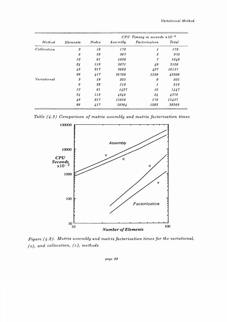
8/13/2019 Richard Jeans 1992 PhD Thesis
http://slidepdf.com/reader/full/richard-jeans-1992-phd-thesis 88/215
Variational Method.
Method Elements Nodes
CPU
Assembly
Timing in seconds
Factorisation
x 1O-
Total
Collocation 3 19 172 1 173
6 33 367 3 370
12 61 1039 7 1046
24 113 3071 49 3120
48 217 9680 457 10137
96 417 36708 5598 42306
Variational 3 19 205 0 205
6 33 518 1 519
12 61 1437 10 1447
24 113 4348 24 437248 217 15258 179 15437
96 417 58364 1205 59569
Table (4.3) Comparison of matrix assembly and matrix factorization times
1UUU(o
10000
CPUSeconds
x10 2
1000
100
1n
Assembly
vc
c
V
Factorisation
IV10
Number of Elements100
Figure (4.2). Matrix assembly and matrix factorization times for the variational,
(v), and collocation, (c), methods
page 88
8/13/2019 Richard Jeans 1992 PhD Thesis
http://slidepdf.com/reader/full/richard-jeans-1992-phd-thesis 89/215
l ariulion(il. 1lcthod.
For those closed geometries there will be problems of uniqueness at interior resonant fre-
quencies and 110method is ii pleiuented to reinme these problems. This is likely to account. for
the breakdown of the numerical results with respect to frequency
sincethe
range of wavenuin-bers over which the numerical problem is ill-conditioned at a critical wavenumber increases wit Ii
frequency until there is an overlap. Loss of accuracy at low frequencies is unlikely to be evident
unless the vavenuiuber is very close to the critical wavenuniber.
Figure (4.3) shows the results calculated using both the variational and collocation method
compared to the analytical solution for a sphere. The 6 element results show high accuracy at
low frequencies with a breakdown of both numerical solutions starting at ka = 2.5. There is
no significant difference in accuracy between the two methods. The 24 element results show
no breakdown of the solutions below ka =5 but the there is slightly better accuracy for the
variational results at the higher frequencies.
Figures (4.4-5) show the two methods compared to the results generated by S.W. Wu s
axisymmet ric method using 20 high order elements applied to prolate and oblate spheroids
respectively. In the case of the prolate spheroid, the breakdown of both numerical results occurs
at the same order of frequencies, and there is no significant difference in accuracy between them.
Since the mesh geometries for the spheroids are simply a scaled spherical mesh, higher accuracy
would be obtained if a more intelligent mesh were used that reflected the geometry and boundary
conditions of the specific spheroid.
For oblate spheroid there is no distinct breakdown of the numerical methods for both mesh
densities. The 24 element case shows high accuracy for all frequencies. For the 6 element case the
accuracy of both methods degenerates at about ka = 3.0 with the variational method showing
slightly higher accuracy.
4.8.2 Flat Disk
Figures (4.7-14) show the numerical calculation of the dimensionless radial surface pres-
sure on a circular disk radiating with constant normal velocity without a baffle. The results
are calculated using the mesh geometries shown in figure (4.6) using both the variational and
collocation methods. The equation for the surface pressure field for a thin shell was presented in
Chapter 2. For a flat continuous surface with no incident wave Eq. (2.5.5) gives a relationship
for the surface pressure,
2ýdý+(P)+0-(P)) _ .Mk[ý](P) = 0. (4.8.2)
page 89
8/13/2019 Richard Jeans 1992 PhD Thesis
http://slidepdf.com/reader/full/richard-jeans-1992-phd-thesis 90/215
Variational Mcihod.
Therefore the dimensionless surface pressure is given by,
2k (D (4.8.3)
an/o
where(11..
represents the constant normal surface velocity. Figure (4.7-10) show the amplitude0
of this quantity and figure (4.11-14) show the phase.
The numerical results are compared to results extracted from work by Weiner [1951], which
were calculated from diffraction data published by Leitner [1949]. Similar results have also been
published by \ Vu, Pierce and Ginsberg [1987] who use an axisymmetric variational procedure.
All results show convergence between 20 and 80 elements and there is little that separates
the accuracy between the collocation and variational methods. Overall there is a high degree
of accuracy. It is clear from these graphs however, that accuracy decreases significantly at the
edges of the disk. The accuracy at the edge does not seem to improve as the density of elements
is increased.
Figures (4.15-16) show the radiation reactance and resistance of the disk calculated using
both the variational and collocation methods. The radiated power and rate of radiation of
kinetic energy for the disk are given by,
11_1
2iwP
Is
JS ondS
(4.8.4)a
ý=1(9
a2k;,ßpsn
dS
The radiation impedance is defined using Eq. (4.8.4) by,
or= or, Ui =11
*(4.8.5)
where 0r is the positive radiation resistance, representing radiation damping, and o-i is the
radiation reactance that is usually positive; representing added fluid mass rather than fluid
damping.
In both figures the numerical results compare well to the results of Weiner [1951] and
Bouwkanip [1941], with a slightly higher degree of accuracy with the variational method. The
page 90

8/13/2019 Richard Jeans 1992 PhD Thesis
http://slidepdf.com/reader/full/richard-jeans-1992-phd-thesis 91/215
Variational.fethod.
resistance results from the work by Bouwkarnp were calculated for the complementary aperture.
The results are plotted on logarithmic scales in figure (4.15) to show the linear low order fre-
quency dependency of the radiation reactance and the higher order frequency dependency of the
radiation resistance.
The final result for the flat disk, figure (4.17), shows the convergence of the radial pressure
amplitude for the three mesh discretizations. The 28 element mesh is distinguished by the high
density of elements near the edge, however all the mesh geometries show similar inaccuracies
at the edge of the plate. To improve the accuracy at the edge of the disk it seams that a more
sophisticated way of imposing the edge boundary condition needs to be developed.
4.8.3 Flat Square Plate
Figure (4.18-19) show the radiation resistance and reactance calculated for the square plate
of side length L. The numerical results are calculated using both the variational and collocation
methods and are compared to the results extracted from work by « arham [1988].
There is good agreement using all methods but the non logarithmic plot shows that there
is higher accuracy with the variational method. The results from \Varham correspond to his
results for an asymptotic fine mesh. Comparison with the results for his `practical mesh show
that there is a significantly higher degree of accuracy and rate of convergence for both the
collocation and variational methods. This would be expected since Warham s method uses a
piecewise constant element discretization.
4.8.4 Terai s Problem
Terai s paper [1980] provides a comparison between his numerical results and an experi-
mental result. Figure (4.20) shows the comparison between the collocation and variation results
and the measured result extracted from Terai s work. The results are the pressure gain in dB
around a rectangular plate due to a point source. The results are calculated at a radius of 0.31
from the origin, in the X-Z plane, and the source is at a distance of 0.5 from the origin along
the Z axis. The rectangular plate in the X-Y plane has dimensions 0.3 x 0.2.
Both the collocation results and the variational results agree well with the measured values,
and show a significantly higher degree of accuracy than Terai s results.
page 91
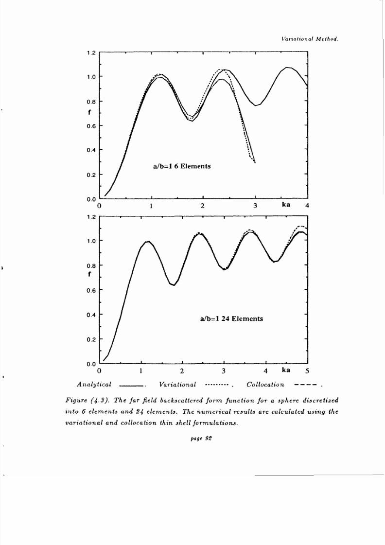
8/13/2019 Richard Jeans 1992 PhD Thesis
http://slidepdf.com/reader/full/richard-jeans-1992-phd-thesis 92/215
Variational Method.
1.2
1.0
0.8
f
0.6
0.4
0.2
nn
a/b=16 Elements
v. v
0
1.2
1.0
1 2 3 ka 4
0.8f
0.6
0.4a/b=124 Elements
0.001234 ka 5
Analytical Variational ---- -- - .Collocation ----
Figure (4.3). The far field backscattered form function for a sphere discretized
into 6 elements and 24 elements. The numerical results are calculated using the
variational and collocation thin shell formulations.
page 92
0.2
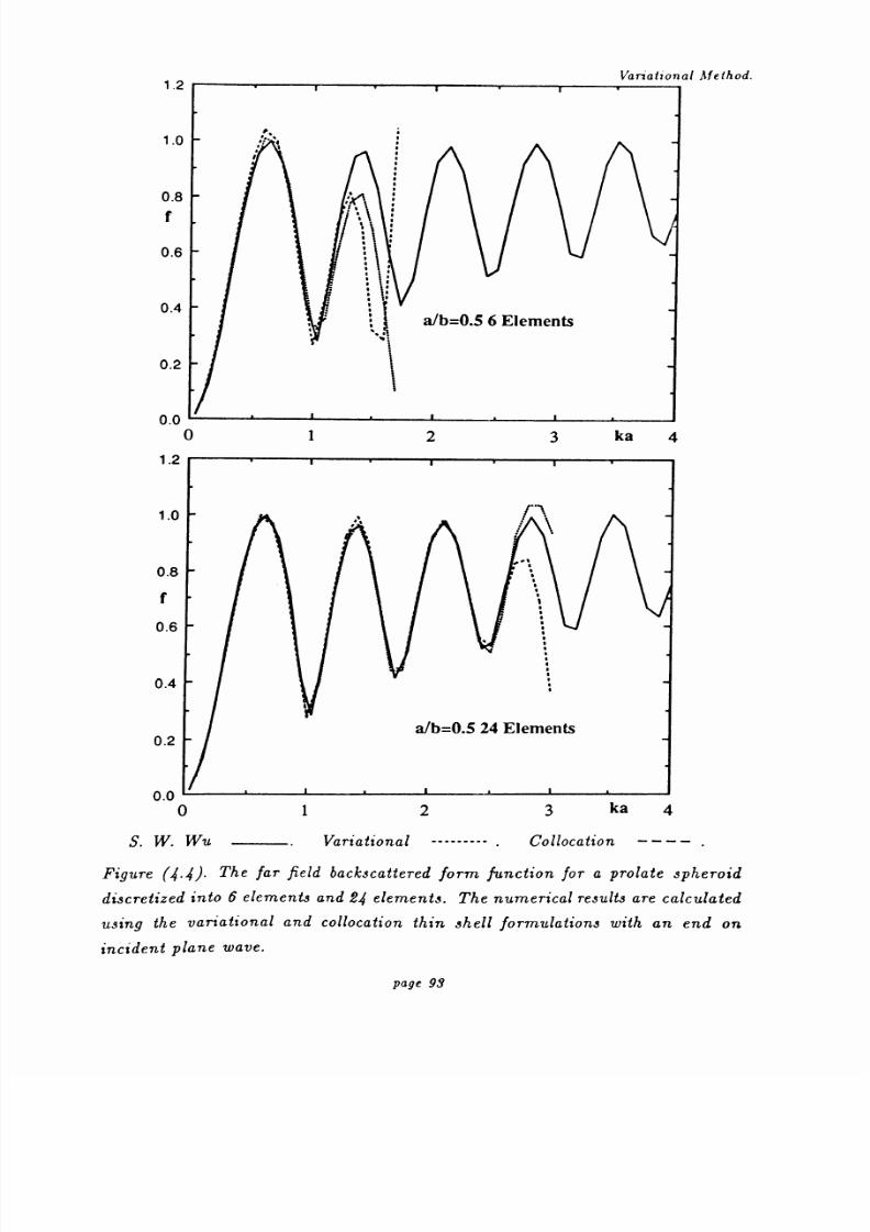
8/13/2019 Richard Jeans 1992 PhD Thesis
http://slidepdf.com/reader/full/richard-jeans-1992-phd-thesis 93/215
1.2
1.0
0.8f
0.6
0.4
0.2
nn
Variational Method.
ii
t
5
alb=0.5 6 Elements
v. v
U
1.2
1.0
0.8
f
0.6
0.4
.,,,
a/b=0.5 24 Elements0.2
0.0 ,0123 ka 4
S. W. Wu variational --------- .Collocation ----
Figure (4.4). The far field backscattered form function for a prolate spheroid
discretized into 6 elements and 24 elements. The numerical results are calculated
using the variational and collocation thin shell formulations with an end on
incident plane wave.
1 2 3 ka 4
page 93
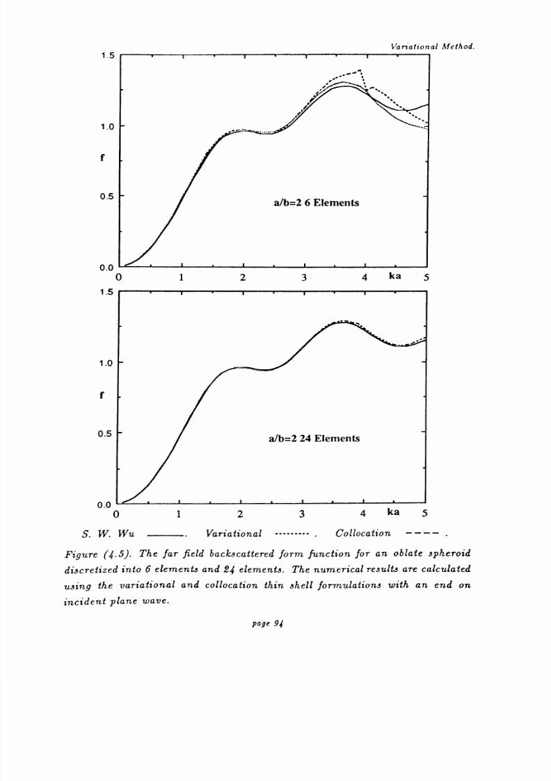
8/13/2019 Richard Jeans 1992 PhD Thesis
http://slidepdf.com/reader/full/richard-jeans-1992-phd-thesis 94/215
Variational bfethod.
1.5
w
. `
ý.0
f
0.5
0.0L0
1.5 r
. -,
1.0
f
0.5alb=2 24 Elements
0.001234 ka 5
S. W. Wu Variational ......... .Collocation ----
Figure (4.5). The far field backscattered form function for an oblate spheroid
discretized into 6 elements and 24 elements. The numerical results are calculated
using the variational and collocation thin shell formulations with an end on
incident plane wave.
a/b=2 6 Elements
1 2 3 4 ka 5
Page 94

8/13/2019 Richard Jeans 1992 PhD Thesis
http://slidepdf.com/reader/full/richard-jeans-1992-phd-thesis 95/215
Variational Method.
a) 20 element disk
c) 80 element disk
b) 28 element disk
d) 36 element plate
e) 24 element Terai problem plate
Figure 4.6). The thin plate mesh geometries
page 95

8/13/2019 Richard Jeans 1992 PhD Thesis
http://slidepdf.com/reader/full/richard-jeans-1992-phd-thesis 96/215
Variational.%ffihod.
2.0
2
IPI 43
.... i
1.0
ka=1
0.00.0 0.2
Wiener.
0.4 0.6
Variational
0.8 r/a 1.0
Figure The dimensionless radial pressure amplitude on a circular disk
radiating with constant normal velocity without a baffle. The variational results
were calculated with one quarter of the disk discretized into 20 elements.
page 96

8/13/2019 Richard Jeans 1992 PhD Thesis
http://slidepdf.com/reader/full/richard-jeans-1992-phd-thesis 97/215
Variational Method.
2.0
IPI
1.0
0.0L-0.0 0.2
Wiener.
0.4 0.6
Variational
0.8 r/a 1.0
Figure 4.8). The dimensionless radial pressure amplitude on a circular disk
radiating with constant normal velocity without a baffle. The variational results
were calculated with one quarter of the disk discretized into 80 elements.
page 97
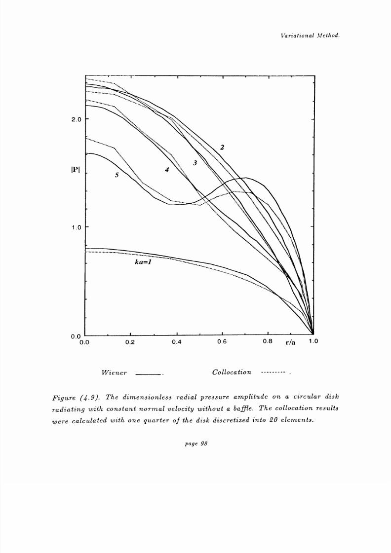
8/13/2019 Richard Jeans 1992 PhD Thesis
http://slidepdf.com/reader/full/richard-jeans-1992-phd-thesis 98/215
Variational Method.
2.0
:::::....:...
2
3IPI
1.0
5
ka=1
4
0.01-0.0 0.2
Wiener.
0.4 0.6 0.8 r/a
Collocation ---------
1.0
Figure (4.9). The dimensionless radial pressure amplitude on a circular disk
radiating with constant normal velocity without a baffle. The collocation results
were calculated with one quarter of the disk discretized into 20 elements.
page 98

8/13/2019 Richard Jeans 1992 PhD Thesis
http://slidepdf.com/reader/full/richard-jeans-1992-phd-thesis 99/215
Variational.fffhod.
2.0
IPI
1.0
0.01 --0.0 0.2
Wiener
0.4 0.6
Collocation
0.8 r/a 1.0
Figure (4.10). The dimensionless radial pressure amplitude on a circular disk
radiating with constant normal velocity without a baffle. The collocation results
were calculated with one quarter of the disk discretized into 80 elements.
page 99

8/13/2019 Richard Jeans 1992 PhD Thesis
http://slidepdf.com/reader/full/richard-jeans-1992-phd-thesis 100/215
Variational.fethod.
90
S
60
30
0
4
3
-30
-60
ka=1
-90 -I0.0 0.2
Wiener.
0.4 0.6 0.8r/a 1.0
Variational --------- .
Figure 4.11). The dimensionless radial pressure phase on a circular disk radiat-
ing with constant normal velocity without a baffle. The variational results were
calculated with one quarter of the disk discretized into 20 elements.
2
page 100
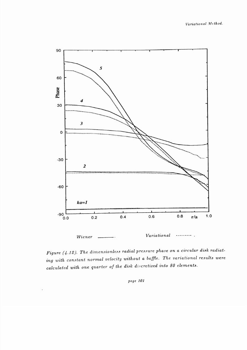
8/13/2019 Richard Jeans 1992 PhD Thesis
http://slidepdf.com/reader/full/richard-jeans-1992-phd-thesis 101/215
Variational Mdhod.
90
5
60
4
0
30
---- ------------............................................................................
...............9
-30
a
-60
ka=l
-900.0 0.2
Wiener
0.4 0.6 0.8 r/a1.0
Variational --------- .
Figure (4.12). The dimensionless radial pressure phase on a circular disk radiat-
ing with constant normal velocity without a baffle. The variational results were
calculated with one quarter of the disk diýcretized into 80 elements.
page 101

8/13/2019 Richard Jeans 1992 PhD Thesis
http://slidepdf.com/reader/full/richard-jeans-1992-phd-thesis 102/215
Gariational Method.
90
5
60
4)
30
0
4
.....
3
1-----1111*1................:::.-30
-60
ka=1
-900.0 0.2
Wiener
0.4 0.6 0.8 r/a 1.0
Collocation --------- .
Figure (4.18). The dimensionless radial pressure phase on a circular disk radiat-
ing with constant normal velocity without a baffle. The collocation results were
calculated with one quarter of the disk discretized into 20 elements.
..
........................................................................................-- ........... ..........
page 102

8/13/2019 Richard Jeans 1992 PhD Thesis
http://slidepdf.com/reader/full/richard-jeans-1992-phd-thesis 103/215
Variational Method.
S
40
a
ý ....
10
4
3
'4.
\ -1
ka=1
-90 `-0.0 0.2
Wiener
0.4 0.6 0.8r/a 1.0
Collocation --------.
Figure (4.14). The dimensionless radial pressure phase on a circular disk radiat-
ing with constant normal velocity without a baffle. The collocation results were
calculated with one quarter of the disk discretized into 80 elements.
page 103

8/13/2019 Richard Jeans 1992 PhD Thesis
http://slidepdf.com/reader/full/richard-jeans-1992-phd-thesis 104/215
l ariational Method.
10
1
.1
01
001
0001
0
0
Variational Collocation --------- .
Bouwkamp ----Wiener O.
Figure 4.15). The radiation impedence of a circular disk radiating with constant
normalvelocity without a baffle. The variational and collocation results were
calculated with one quarter of the disk discretized into 20 elements. The results
are plotted on a logarithmic scale to highlight the low frequency dependence.
page 104
11 ka 10

8/13/2019 Richard Jeans 1992 PhD Thesis
http://slidepdf.com/reader/full/richard-jeans-1992-phd-thesis 105/215
Variational affthod.
1.5
resistance
ý,,,.~ýý
v,.ir..
1.0
i
0.5
ýd.
reactance
I
0.0 `0 246 ka 8
Variational Collocation--------- .
Bouwkamp Wiener O.
10
Figure (4.16). The radiation impedance of a circular disk radiating with constant
normal velocity without a baffle. These are the same results as the previous figure
but plotted on a linear scale.
page 105
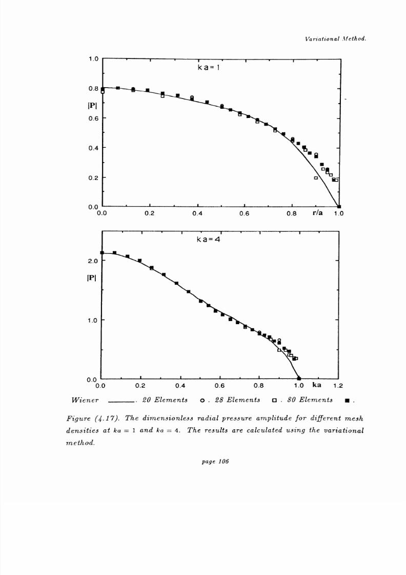
8/13/2019 Richard Jeans 1992 PhD Thesis
http://slidepdf.com/reader/full/richard-jeans-1992-phd-thesis 106/215
Variational Method.
1.0
ka= 1
0.8
IPI
0.6
0.4
0.2
0.0-
0.0
3k
Di
ka=4
2.0
IPI
1.0
a
0.00.0 0.2 0.4 0.6 0.8 1.0 ka 1.2
Wiener.
20 Elements o. 28 Elements o. 80 Elements .
Figure /x.17). The dimensionless radial pressure amplitude for different mesh
densities at ka =1 and ka = 4. The results are calculated using the variational
Method.
0.2 0.4 0.6 0.8 r/a 1.0
page 106
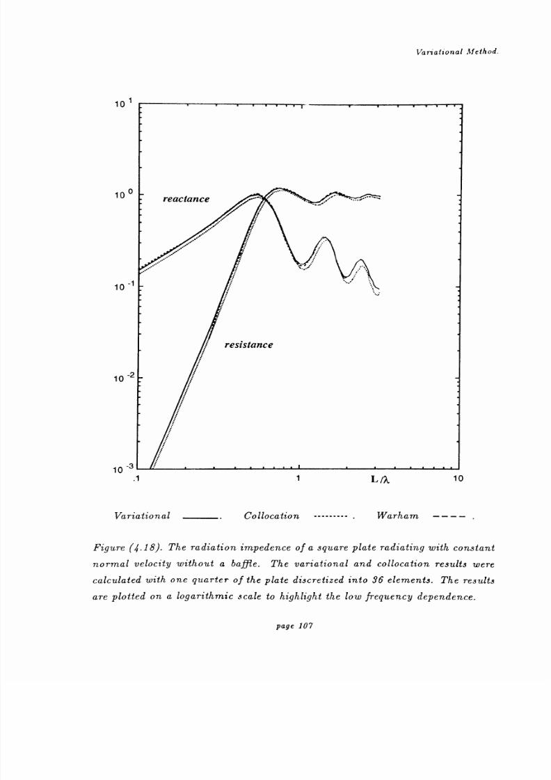
8/13/2019 Richard Jeans 1992 PhD Thesis
http://slidepdf.com/reader/full/richard-jeans-1992-phd-thesis 107/215
Variational Method.
10 1
100
10-1 ;ý
resistance
10 -2
10
.1
Variational
1L /ý 10
Collocation --------- .Warham ----
Figure 4.18). The radiation impedence of a square plate radiating with constant
normal velocity without a baffle. The variational and collocation results were
calculated with one quarter of the plate discretized into 36 elements. The results
are plotted on a logarithmic scale to highlight the low frequency dependence.
reactance
page 107

8/13/2019 Richard Jeans 1992 PhD Thesis
http://slidepdf.com/reader/full/richard-jeans-1992-phd-thesis 108/215
Variational Method.
1.5
1.0
0.5
An
r
. reactance
i
resistance
f.
ýrý
U.V0 L/%, 3
Variational Collocation --------- .Warham ----
Figure (1.19). The radiation impedance of a square plate radiating with constant
normal velocity without a baffle. These are the same results as the previous figure
but plotted on a linear scale.
page 108

8/13/2019 Richard Jeans 1992 PhD Thesis
http://slidepdf.com/reader/full/richard-jeans-1992-phd-thesis 109/215
Variational Method.
4
dB
I.;
0 I
-4 `0
Source
90 180 270 0 360
Microphone
Measured Variational --------- .Collocation
----
Figure (4.20). Nearfield pressure gain for a point source wave scattered by a
rectangular plate at k= 18.44. The numerical results are calculated using 24
elements and the measured result is extracted from the work by Terai.
page 109
iv
8/13/2019 Richard Jeans 1992 PhD Thesis
http://slidepdf.com/reader/full/richard-jeans-1992-phd-thesis 110/215
The Superposition Method.
CHAPTER 5.
The Superposition Method
5.1 Introduction
Superposition methods have long been used as a bench test for other numerical analyses of
acoustic fields. Recently Koopmann Song and Fahnline [1989] suggested that a superposition
method could be extended into a general solution technique for calculating acoustic fields. In
the work of Koopmann et a1[1989] Song et al [1991] and Miller et aI [1991] a complex radiator
is replaced by an array of simple monopole sources of unknown magnitude constrained to lie on
a surface interior to the body of the radiator. The magnitude of the simple sources is calculated
by equating the normal velocity prescribed on the surface of the radiator to that generated by
the array of simple sources. This is performed at the same number of points as there are simple
sources and consequently a system of equations is generated. The solution of this equation set
gives the magnitude of the simple sources and from these values an exterior pressure field can
be calculated.
Since the superposition method removes the need for singular integration techniques is
has been suggested that the method improves on the traditional BEM. The author however
supports the view of Katz [1987] who suggests that some [superposition] methods spoil the
whole approach ...they will work with some cases but are not general and they will produce
ill conditioned systems in some cases. It was decided that the superposition method was worth
investigating in order to establish that in a hierarchy of integral methods the BEM represents
the limit in terms of accuracy and conditioning of the superposition method.
Although the superposition method described above circumvents the problem of uniqueness
of solution found in BEMs a formulation which constrains the interior point sources to be on
an interior surface does become ill-conditioned at another set of critical wavenutnbers. These
wavenumbers correspond to the eigenvalues of the unrelated Dirichlet problem interior to the
source surface. The superposition integral is now equivalent to a single layer source distribution
and as such can be shown to have a non-unique solution at these eigenvalues. Although it is
possible to reduce the interior source surface so that any critical wavenumbers lie outside the
frequency range of interest there is also a potential loss in numerical stability. In this chapter
a numerical strategy will be presented that circumvents this uniqueness problem allowing the
page 110
8/13/2019 Richard Jeans 1992 PhD Thesis
http://slidepdf.com/reader/full/richard-jeans-1992-phd-thesis 111/215
The Superposition Method.
optimum choice of interior surface to be made, in order to obtain the maximum improvement
in numerical stability of the solution.
The problem of uniqueness has been overcome in this study by considering the superposition
integral in terms of a hybrid combination of single and double layer potentials. A similar solution
to the problem of uniqueness in B.E..N1 s is discussed by Filippi [1977], and Colton and Kress
[1983].
As noted by Koopmann et al [1989] it is possible to use derive a superposition integral either
by assuming that the source distribution and Green s function are constant over each interior
element or by allowing the source distribution and the Green s function to vary in some manner
and the kernel function to be evaluated using Gaussian quadrature. In this paper the first
method is denoted as the Point source Superposition Method (PSNI). Results are also presented
for the second method which is denoted as the Integrated source Superposition Method (ISM);
the source distribution and geometry are approximated by the use of quadratic interpolation
functions defined using 9 noded surface elements.
5.2 The Superposition Integral
For a body radiating with a prescribed surface velocity it is desirable to calculate the exterior
pressure field. The principle of wave superposition shows that the acoustic solution for some
radiating body is equivalent to the acoustic solution of some source distribution interior to the
body. If both systems satisfy the same Neumann boundary condition on the surface of the body
then the pressure distributions generated by both are equivalent since an exterior pressure field
is unique for a prescribed boundary condition. Koopmann et al proposed that the solution of
the equivalent superposition formulation of a problem offers many significant advantages over a
B. E. M solution of the same problem. The validity of the superposition method can be shown in
the following way.
Consider a continuous distribution of sources contained in a volume Q. This source distri-
bution is interior to a closed fictitious surface S on which there is a prescribed normal velocity
distribution u,,. The volume enclosed by S is denoted D and the volume exterior to S is denoted
E. This geometry is shown in figure (5.1).
page 111

8/13/2019 Richard Jeans 1992 PhD Thesis
http://slidepdf.com/reader/full/richard-jeans-1992-phd-thesis 112/215
The Superposition Method.
E
S
Figure (5.1). . The geometry for formulating the superposition integral.
Applying the principle of mass conservation (Pierce [1989] Chapter 4 p162) to the volume
enclosed by S leads to a modified reduced wave equation defined by,
v2 p(r) + k2P(r) = iwpgo(r), rED. (5.2.1)
A time dependence of e-'wt is assumed and qo(r) is the interior source strength defined by,
q(r) rES2,
qo(r) = (5.2.2)
0 rEDexcluding ft
Using Eq. (5.2.1) the modified interior Helmholtz integral equation can be developed in a similar
way to the standardinterior Helmholtz
equation andis
givenby,
ýiwpu(ro)Gk(r, ro) - p(ro)
öGk
ö
(nr,ro) d'Sr, + iwp4(ro)Gk(r, ro)dVraJs ra
fn(1
- c(r))(r)p(r),
Gk (r, ro) =1eikr
47rrT=
IT- vol
(5.2.3)
The unrelated exterior Helmholtz equation is independent of the interior source distribution and
identical to the exterior Helmholtz equation for a real surface S with prescribed normal velocity
distribution u,,. This equation is defined by,
page 112

8/13/2019 Richard Jeans 1992 PhD Thesis
http://slidepdf.com/reader/full/richard-jeans-1992-phd-thesis 113/215
The,cuperpositaon Method.
ÖGk(r, ro)
SPro)
a 1.ý pun(ro)Gk dS ro = C(r )P(r ). (5.2.4)
n*o
In the source distribution model of the vibrating body, the surface S is a construction
indicating where the normal velocity distribution is prescribed. Consequently the pressure and
velocity distributions across the surface must, be continuous. When r is taken to be on S, Eq.
(5.2.3) and Eq. (5.2.4) combine to give,
P(r) =fipq(ro)Gk(r,
ro)dVro. (5.2.5)
Eq. (5.2.5) is the superposition integral. Associated with this equation is its differentiated form,
defined by,
2dn(r) =
In
q(ro)ÖG3(ro d\0.
0
5.3 Uniqueness
(5.2.6)
In the derivation of Eq. (5.2.5) and Eq. (5.2.6) the Helmholtz integral equations are cir-
cumvented and for a source domain that contains no interior volume, numerical implementations
of these equations are unique at all frequencies. However the choice of volume S2 s arbitrary
and for ease of numerical implementation it is best to locate the interior source distribution
over an interior surface S of small thickness 6r. However the superposition integral will now
exhibit non-uniqueness at critical wave numbers. This non-uniqueness can be demonstrated in
the following manner.
For the case where Sl is chosen to be a thin shell, Eq. (5.2.5) and Eq. (5.2.6) become,
P(r) =I iwpq(ro)Gk(r, ro)brrdSfo. (5.3.1)IS/
un(r) =J 4(ro)8GO(r ro)
brdS;.o.
(5.3.2)is,
o
page 113
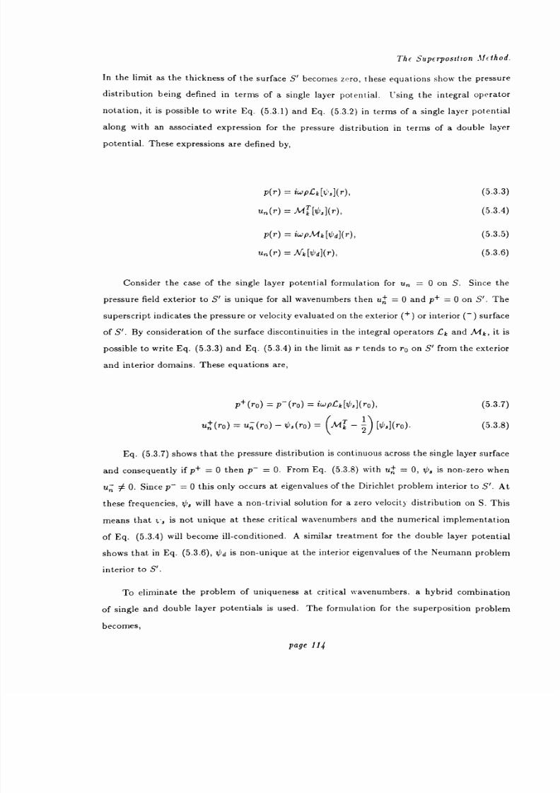
8/13/2019 Richard Jeans 1992 PhD Thesis
http://slidepdf.com/reader/full/richard-jeans-1992-phd-thesis 114/215
The Superposition Method.
In the limit as the thickness of the surface S' becomes zero, these equations show the pressure
distribution being defined in terms of a single layer potential. Using the integral operator
notation,it is
possibleto
writeEq. (5.3.1)
andEq. (5.3.2) in
terms of a singlelayer
potential
along with an associated expression for the pressure distribution in terms of a double layer
potential. These expressions are defined by,
P(r) - iwpCk[ 's](r), (5.3.3)
u(r) = Mk [t3](r), (5.3.4)
P(r) = 2Wp ik [11d](r), (5.3.5)
um(r) _Yk[0d](r), (5.3.6)
Consider the case of the single layer potential formulation for u =0 on S. Since the
pressure field exterior to S' is unique for all wavenumbers then u, =0 and p+ =0 on S. The
superscript indicates the pressure or velocity evaluated on the exterior (+) or interior (-) surface
of S'. By consideration of the surface discontinuities in the integral operators Gk and Mk, it is
possible to write Eq. (5.3.3) and Eq. (5.3.4) in the limit as r tends to r0 on S' from the exterior
and interior domains. These equations are,
p+(ro) = P-(r0) = iwprk[0, ](ro), (5.3.7)
un (ro) = um(ro)- 0s(ro) =
(Mr
-2{ s](ro).(5.3.8)
Eq. (5.3.7) shows that the pressure distribution is continuous across the single layer surface
and consequently if p+ =0 then p- = 0. From Eq. (5.3.8) with u,+, = 0, v, is non-zero when
un # 0. Since p- =0 this only occurs at eigenvalues of the Dirichlet problem interior to S. At
these frequencies, 0, will have a non-trivial solution for a zero velocity distribution on S. This
means that t,,, is not unique at these critical wavenumbers and the numerical implementation
of Eq. (5.3.4) will become ill-conditioned. A similar treatment for the double layer potential
shows that in Eq. (5.3.6), 1d is non-unique at the interior eigenvalues of the Neumann problem
interior to S.
To eliminate the problem of uniqueness at critical wavenumbers, a hybrid combination
of single and double layer potentials is used. The formulation for the superposition problem
becomes,
page 114

8/13/2019 Richard Jeans 1992 PhD Thesis
http://slidepdf.com/reader/full/richard-jeans-1992-phd-thesis 115/215
The Superposition.1Method.
P(?) = iwp(. Ck + iTlMk) [v,7(r), (5.3.9)
utz(r) = (Mk + ii \ (5.3.10)
The value of the real constant 77n Eq. (5.3.9) and Eq. (5.3.10) is chosen to be 1/k to compensate
for the order of frequency terms in the integral operators. The advantage of the superposition
method using this hybrid formulation is that there is no high order singularity in the .A operator
since the source surface S is not coincident with the boundary surface S. It should be noted
however that in regions where there is a high density of critical wavenumbers, a high degree of
accuracy is needed to reduce the range of wav-enumbers over which the non-hybrid operators are
ill-conditioned, so that the hybrid formulation is efficient.
5.4 Numerical Formulation
A numerical implementation of the superposition integral has several advantages over a
BEM. A major factor in any BEM is the numerical treatment of the singularities that inevitably
occur in the formulation. In the superposition method the source distribution is interior to the
body and therefore not coincident. Consequently there is no singularity in the Green s function
of Eq. (5.3.9) and Eq. (5.3.10).
In Eq. (5.3.9) and Eq. (5.3.10) the surface S can be discretized into a number of elements,
n. The nodes of the interior source elements must each have a corresponding surface node. Using
the definitions of previous researchers the corresponding node on the interior source surface is
known as the self node. This definition can be extended to refer to the self element which
is thesource
surface element that contains the self node. Eq. (5.3.10) can be approximated
numerically by,
n
1ý,Gk(r, ro) 02Gk(r. ro)
un(r) =E -ý 7(ro)dSro7=1m Ö12ranr.
For the PSM it is assumed that the kernel of Eq. (5.4.1) and (r0) is constant within the
element and it can be written in matrix form by,
{un} = DA{ ;}, (5.4.2)
page 115

8/13/2019 Richard Jeans 1992 PhD Thesis
http://slidepdf.com/reader/full/richard-jeans-1992-phd-thesis 116/215
The Supfrposition.Method.
With,
r"n; r-ni r. nj Gk(r) Ge(r)Dij = Gk(r)
r+i77
rr
(G(r)
-T-r 7zß.nj C . 4.3)
r=ri - rj. r=Irl.
and A is the diagonal area matrix.
In Eq. (5.4.2) {u} is the vector containing the n values of u evaluated at the points r;
on the boundary surface that correspond to the n nodal points defined on the interior surface,
rj. The source surface nodal points are defined at the centroid of the source surface element.
The vector {0} contains the n values of ý,j evaluated on the interior source surface and .
4j ,
corresponds to the amplitude of point source radiators situated at the interior nodal positions.
The discretized form of Eq. (5.3.9) is defined in a similar way to Eq. (5.4.2),
{p}-
(5.4.4)
with,
r"njM; j = Gk(r) + iriG' (r) (5.4.5)
r
Eq. (5.4.2) and Eq. (5.4.4) can be combined to give an expression for p in terms of ums,. his is
written as,
{p} = MD-1{u} (5.4.6)
In the PSM the principal assumption is that the interpolation of the source distribution is
given by,
V= b(ro, rj)Zj, (5.4. i)
where 6(ro, rj) is one at the nodal point defining the element and zero otherwise, and V)j is the
nodal value of the source distribution for the element. For the ISM a different assumption is
made. Within the element the source distribution is given by.
page 116

8/13/2019 Richard Jeans 1992 PhD Thesis
http://slidepdf.com/reader/full/richard-jeans-1992-phd-thesis 117/215
Thf Superposition Method.
VI)= {1Ve}T{ a}, (5.4.8)
where {Ne} is the vector of element shape functions and {ýJ} is the vector of element nodal
values of the source distribution. The numerical approximation given by Eq. (5.3.10) now
becomes,
un(T) -
(ýGk(rro)
+ .ýa2GkI. Te}TdSr°{2J}. (5.4.9)S
Onr (9nrOnrJ=1 ý°
The numerical integration in Eq. (5.4.9) can be performed using simple Gaussian quadrature
since there is no singularity for retracted source surfaces. A matrix equation set can be assembled
for the acoustic formulation eliminating 0, the global vector of nodal source strengths,
{p} = MIDI'{un} (5.4.10)
In this study the interior nodal points for both the PSM and ISM were generated in the
same way. Since only the nodal point for the element is needed in the PSM, these nodal points
can correspond to the nodal points for the ISM. To optimize the conditioning of the D and DI
matrices, the definition of the boundary and source surface nodal points is critical. Following
previous work the interior source points are defined by,
Tj = Ti -d1
2, (5.4.11)
where d is defined as the retraction distance. The relationship in Eq. (5.4.11) is not sufficient
to ensure optimum conditioning. The boundary nodal points have to be defined so that,
.ITi
-TjIj,
4i > ITi-'I=i (5.4.12)
These relationships ensure that there is optimum symmetry and diagonal dominance of the
equation set. This requirement is important in reducing the degree of ill conditioning of the
formulation, however such a restriction on the positioning of the boundary surface nodal points
will be independent of the applied boundary conditions.
page 117

8/13/2019 Richard Jeans 1992 PhD Thesis
http://slidepdf.com/reader/full/richard-jeans-1992-phd-thesis 118/215
The Super position Method.
For radiation problems u is simply the prescribed surface normal velocity. For plane wave
scattering u1. can be shown (Junger and Feit [1986]) to be equal to,
PI-
&I r
wp(5.4.13)
where uj is the fluid particle velocity on the boundary surface in the absence of any interior
source distribution, generated by the incident pressure wave. The incident pressure wave has
amplitude pl. and wave vector kI.
5.4.1 Matrix Condition Number
A well recognized failing of the superposition method is the ill conditioning of the generated
matrices. This lack of conditioning is due to the numerical instability of Fredholm equations of
the first kind (Arfken [1985], Miller [1974]). One loss of conditioning is due to the loss of diagonal
dominance as the source surface is retracted from the boundary surface. Computationally the
loss of conditioning means that small changes in the surface velocity distribution can have a
large effect on the source distribution. Following Golub and Van-Loan [1983] a conditioning
number can be calculated that gives a measure of the sensitivity of a linear system. The matrix
problem for the PSM or ISM can be stated as,
{un}= D{O}. (5.4.14)
If the boundary velocity distribution is perturbed by an amount {6u } then for this linear
system,
{b} = D-1{bu, }, (5.4.15)
and from the properties of vector and matrix norms,
11 11< JID-111
16un11(5.4.16)1011 11011
tun II IIDIIIIVII. (5.4.1 7)
page 118
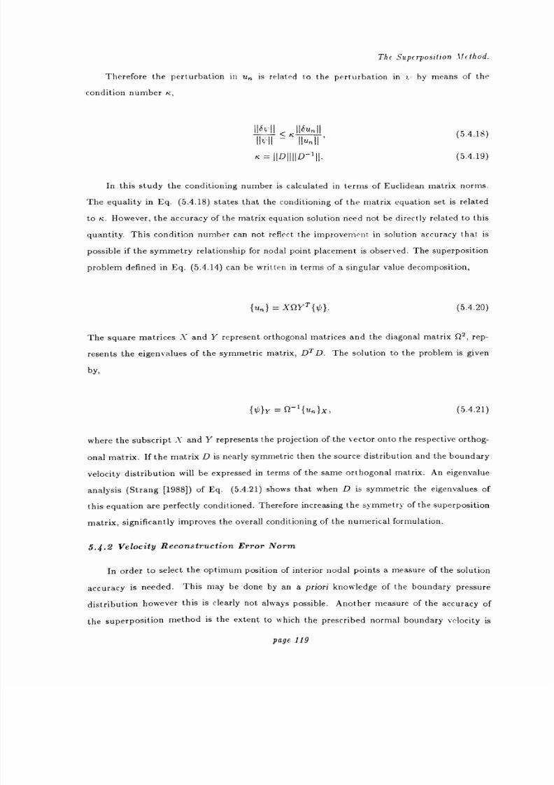
8/13/2019 Richard Jeans 1992 PhD Thesis
http://slidepdf.com/reader/full/richard-jeans-1992-phd-thesis 119/215
The Superposition.11Eihod.
Therefore the perturbation in un is related to the perturbation in L- by means of the
condition number n;,
IIa'+'II<K
IIbun II(5.4.18)
IIv'II IIti II
= IIDIIIID-111. (5.4.19)
In this study the conditioning number is calculated in terms of Euclidean matrix norms.
The equality in Eq. (5.4.18) states that the conditioning of the matrix equation set is related
to t;. However, the accuracy of the matrix equation solution need not be directly related to this
quantity. This condition number can not reflect the improvement in solution accuracy that is
possible if the symmetry relationship for nodal point placement is observed. The superposition
problem defined in Eq. (5.4.14) can be written in terms of a singular value decomposition,
{un} = XS2YT {b} (5.4.20)
The square matrices X and Y represent orthogonal matrices and the diagonal matrix Q2, rep-
resents the eigenvalues of the symmetric matrix, DT D. The solution to the problem is given
bY,
lo}Y =Q-lf, un}X, (5.4.21)
where the subscript X and Y represents the projection of the vector onto the respective orthog-
onal matrix. If the matrix D is nearly symmetric then the source distribution and the boundary
velocity distribution will be expressed in terms of the same orthogonal matrix. An eigenvalue
analysis (Strang [1988]) of Eq. (5.4.21) shows that when D is symmetric the eigenvalues of
this equation are perfectly conditioned. Therefore increasing the symmetry of the superposition
matrix, significantly improves the overall conditioning of the numerical formulation.
5.4.2 Velocity Reconstruction Error Norm
In order to select the optimum position of interior nodal points a measure of the solution
accuracy is needed. This may be done by an a priori knowledge of the boundary pressure
distribution however this is clearly not always possible. Another measure of the accuracy of
the superposition method is the extent to which the prescribed normal boundary velocity is
page 119

8/13/2019 Richard Jeans 1992 PhD Thesis
http://slidepdf.com/reader/full/richard-jeans-1992-phd-thesis 120/215
Thf Superpo. iiion .110hod.
reconstructed by the source distribution. By using the numerical approximations of either the
PS-N1or ISM the reconstructed surface normal velocity is given by,
it,, (r) = {D(r)}T D-1{ u, }. (5.4.22)
When r corresponds to a boundary surface nodal point, Ti, then clearly,
(5.4.23)
For other points there will however be some difference in the prescribed and calculated surface
normal velocities and a measure of this difference is the velocity reconstruction error norm,
Ilun- unllo
Ilun llo
where,
(5.4.24)
un -it ll, =
j(u-
-(5.4.25)
This error norm will be closely linked to the error in the boundary surface pressure and can
be used to select the optimum interior nodal positions without an a priori knowledge of the
boundary surface pressure distribution.
5.5 Numerical Results
The superposition formulations were applied to spherical and spheroidal scattering and
radiation problems. These boundary surfaces were chosen due to the cylindrical symmetry that
exists for appropriate boundary conditions. In all cases one quarter of the boundary surface
is discretized, making use of the problem symmetry to reduce the problem size. In order to
optimize the symmetry of the resulting superposition matrices the surface nodal points are
distributed as evenly as possible over the boundary surface.
Figure (5.2) contrasts the non uniqueness characteristics at critical wavenumbers of the
single and double layer formulations with that of the hybrid formulation. A constant normal
velocity distribution is prescribed for a sphere with radius a and the source surface is retracted
page 120
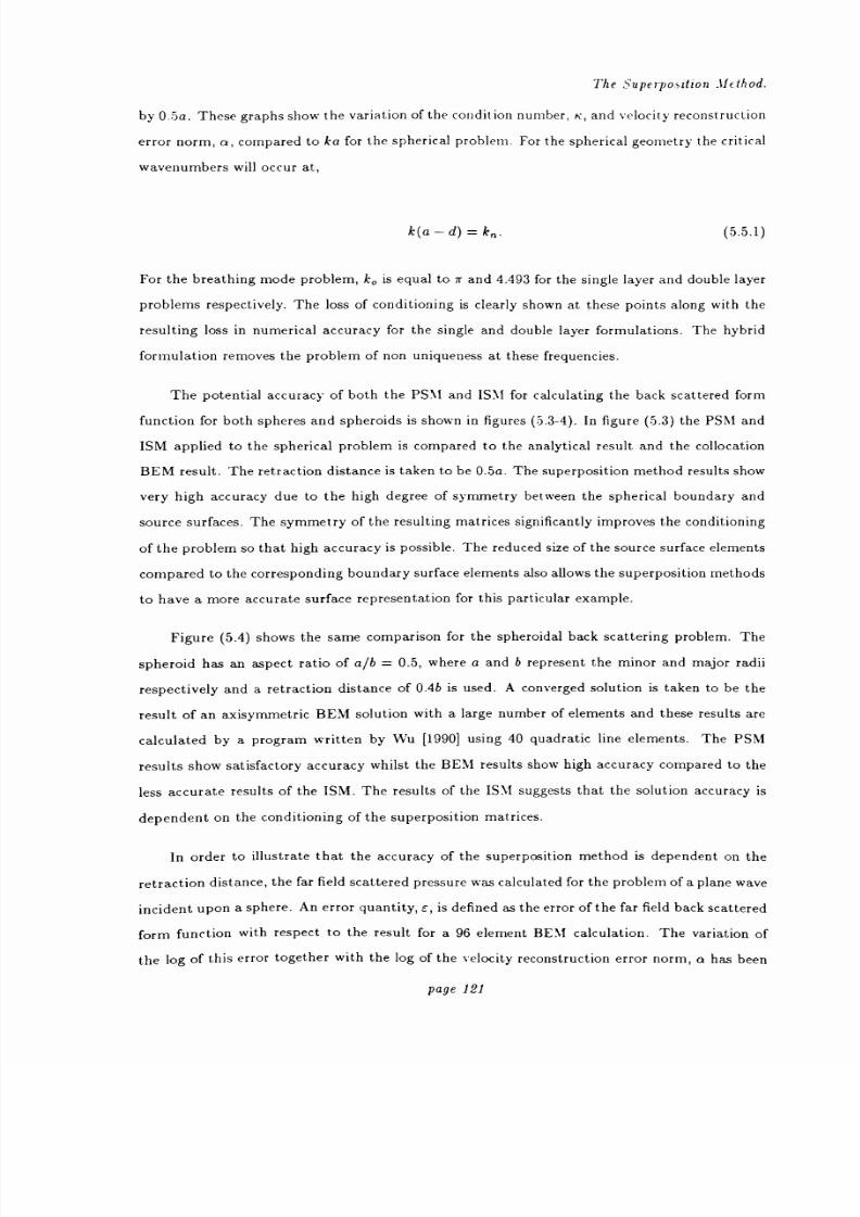
8/13/2019 Richard Jeans 1992 PhD Thesis
http://slidepdf.com/reader/full/richard-jeans-1992-phd-thesis 121/215
The Superposition J10hod.
by 0.5a. These graphs show the variation of the condition number, n, and velocity reconstruction
error norm, a, compared to ka for the spherical problem. For the spherical geometry the critical
wavenumbers will occur at,
k a - d) = kn. 5.5.1)
For the breathing mode problem, ko is equal to it and 4.493 for the single layer and double layer
problems respectively. The loss of conditioning is clearly shown at these points along with the
resulting loss in numerical accuracy for the single and double layer formulations. The hybrid
formulation removes the problem of non uniqueness at these frequencies.
The potential accuracy of both the PSM and ISM for calculating the back scattered form
function for both spheres and spheroids is shown in figures 5.3-4). In figure 5.3) the PSNN1and
ISM applied to the spherical problem is compared to the analytical result and the collocation
BEM result. The retraction distance is taken to be 0.5a. The superposition method results show
very high accuracy due to the high degree of symmetry between the spherical boundary and
source surfaces. The symmetry of the resulting matrices significantly improves the conditioning
of the problem so that high accuracy is possible. The reduced size of the source surface elements
compared to the corresponding boundary surface elements also allows the superposition methods
to have a more accurate surface representation for this particular example.
Figure 5.4) shows the same comparison for the spheroidal back scattering problem. The
spheroid has an aspect ratio of alb = 0.5, where a and b represent the minor and major radii
respectively and a retraction distance of 0.4b is used. A converged solution is taken to be the
result of an axisymmetric BEM solution with a large number of elements and these results are
calculated by a program written by Wu [1990] using 40 quadratic line elements. The PSM
results show satisfactory accuracy whilst the BEM results show high accuracy compared to the
less accurate results of the ISM. The results of the ISM suggests that the solution accuracy is
dependent on the conditioning of the superposition matrices.
In order to illustrate that the accuracy of the superposition method is dependent on the
retraction distance, the far field scattered pressure was calculated for the problem of a plane wave
incident upon a sphere. An error quantity, E, is defined as the error of the far field back scattered
form function with respect to the result for a 96 element BEM calculation. The variation of
the log of this error together with the log of the velocity reconstruction error norm, a has been
page 121

8/13/2019 Richard Jeans 1992 PhD Thesis
http://slidepdf.com/reader/full/richard-jeans-1992-phd-thesis 122/215
The SupErposition Method.
plotted in figure 5.5) as a function of d/a, for a ka = 1. Figure 5.5a) shows the results for the
point superposition method and figure 5.5b) for the integrated superposition method.
The condition number of the solution matrix for both superposition methods is given in
figures 5.6a) and 5.6b). The results for the spherical and spheroidal geometries are presented.
Comparsion of the error measures in figure 5.5a) with the condition number of the matrix
generated with the spherical P5M1 in figure 5.6a) indicates little correspondence between these
quantities. As the velocity reconstruction error norm, a is less than the far field error, the ma-
trices are conditioned such that the accuracy is dependent only on the order of the interpolation
of the source distribution. As the source surface is moved closer to the boundary surface, both
error quantities increase until the velocity reconstruction error norm, a is greater than the error
in the far field back scattered form function, F.
The results for the ISM, shown in figure 5.5b), indicate that between d/a = 0.9 and 0.5 the
trend in the conditioning of the problem, shown in figure 5.6b) and the error indicators a and e is
similiar. For this range of retraction distances the degree of symmetry in the problem increases,
until at about d=0.5 the problem became sufficiently well-conditioned to allow very accurate
solutions to be attained. The far field error, a, increases as d tends to zero, while the error in
the internodal velocity reconstruction remains small. The accuracy in the formulation could be
increased for these low retraction ratios by simply using the singular integration techniques used
in the BEM.
The velocity reconstruction error, a, and the far field back scattered form function error,
e, were also calculated for the spheroidal problem. The values of a and e were calculated as a
function of d/b at kb =1 for both the point superposition and integrated superposition methods.
The results are given in figures 5.7-8). For both methods the variation of a is similar, revealing
a minimum for a particular retraction ratio, before the numerical error due to small d became
significant. The value of d/b where this occurs decreases with increasing n. The errors for the
PSM show there is a greater range of retraction distances over which there is low error reflecting
the greater symmetry of the corresponding superposition matrices.
5.6 Conclusion
A numerical solution to acoustic problems has been described along with a strategy to
overcome problems of uniqueness using a hybrid formulation. The superposition formulation
was shown to be valid and the breakdown of the numerical formulation at the eigenvalues of
page 122

8/13/2019 Richard Jeans 1992 PhD Thesis
http://slidepdf.com/reader/full/richard-jeans-1992-phd-thesis 123/215
Thf Superposition Method.
the interior source surface was demonstrated. The accuracy of the formulation was measured
through use of a velocity reconstruction error norm.
The numerical results of the superposition method applied to radiation and scattering
problems are presented for spherical and spheroidal surfaces. The numerical results indicate
that with careful choice of boundary and source surface nodal points that it is possible to attain
solutions with high accuracy to both classes of problems. The results demonstrate that the
accuracy of the superposition method unlike the surface integral approaches depends to a
significant degree on the conditioning of the problem rather than the accuracy of the source
representation.
It should be noted that both formulations tested are numerical approximations to Fredholm
equations of the first kind and therefore subject to a inherent instability in the solution process.
As demonstrated in the results the conditioning of the formulation will deteriorate as as the
source surface surface is retracted from the boundary surface. Despite the deterioration of the
condition number accurate solutions are possible for a certain range of retraction distance
however once out of this range large errors occur in the calculated nodal surface velocities.
The numerical conditioning of the problem can be optimized by reducing the source sur-
face retraction distance and therefore increasing the diagonal dominance of the formulation.
However as the surface retraction distance is reduced close to the boundary surface then the
solution accuracy will deteriorate once again due to the inadequate integration of the source sin-
gularity. Another factor that will increase the conditioning of the formulation thus for specific
problems giving a high solution accuracy is the degree of symmetry in the resulting equation
set. However as noted by Song et aI [1991] the symmetry of the formulation will depend on the
surface nodal points the retraction distance and the interpolation of the source distribution.
The numerical experiments indicate that for optimal solution accuracy and problem con-
ditioning then the source nodal points need to be placed at a fixed distance along the normal
from the boundary nodal points. If the source nodal points are placed at any other locations
then a dramatic loss of solution accuracy will occur.
The results also indicate that in order to make the solution accuracy solely dependent on
the discretization of the problem while optimizing the numerical conditioning of the formulation
then the boundary and source surfaces need to be coincident.
page 123

8/13/2019 Richard Jeans 1992 PhD Thesis
http://slidepdf.com/reader/full/richard-jeans-1992-phd-thesis 124/215
The Sunervosition.Method.
8
6
4
2
0
-2
-46. ý
6
4
2
0
-2
A
Single layer
K0
OOOOOOO00000000000
a
78 6.280 6.282 6.284 6.286 ka 6.288
Double layer
OK
O0OOOO
a
''''''
-It8.982 8.984 8.986 8.988 ka 8.990
Figure (5.2). The effect of the hybrid formulation on the elimination of criti-
cal wavenumbersfor
the single layer and double layer PSMformulations.
The
results are for a sphere with constant normal velocity distribution and d=0.5.
The solid line represents the hybrid formulation.
page 124
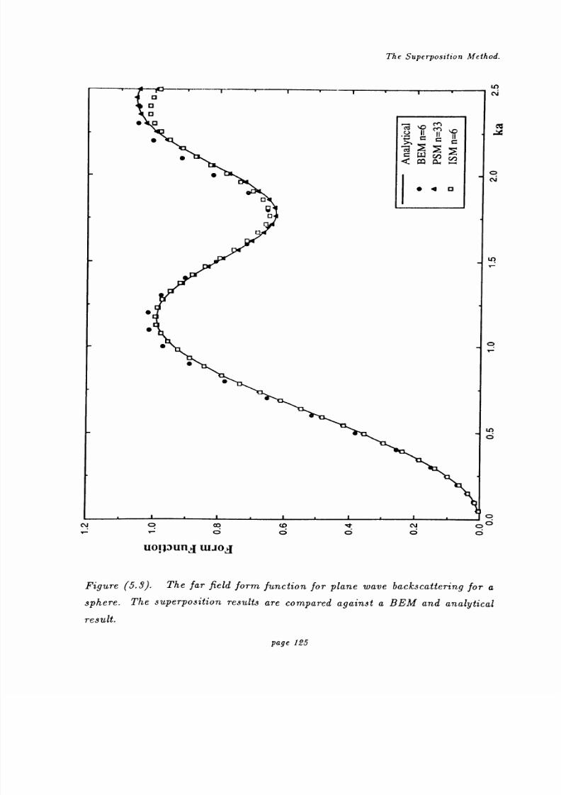
8/13/2019 Richard Jeans 1992 PhD Thesis
http://slidepdf.com/reader/full/richard-jeans-1992-phd-thesis 125/215
The Superposition Method.
aa
aaM
il>, C
C wCn
¢ as a º..,
a
13
N
SC
0N
LO
1:
O
r
LC)6
PNO 00 CO It NOO
ÖÖÖOO
uorppun WJod
Figure (5.3). The far field form function for plane wave backscattering for a
sphere. The superposition results are compared against a BEM and analytical
result.
page 125
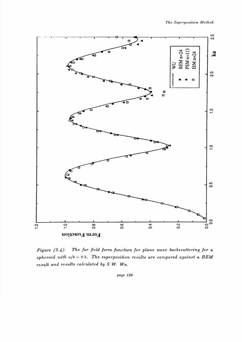
8/13/2019 Richard Jeans 1992 PhD Thesis
http://slidepdf.com/reader/full/richard-jeans-1992-phd-thesis 126/215
The Superposition Method.
aad
134
13
m13
0a
4 1340
a
U,N
Gý
.1
0
N
LO
0
C3
L6
NOcO
uoip: un,4 W. o,4
c0Ö
IT6
MN
NC
3 M a .
0 4 a
N6
J°o°0
Figure 5.4). The far field form function forplane wave
backscattering for
aspheroid with a/b = 0.5. The superposition results are compared against a BEM
result and results calculated by S. W. Wu.
page 126

8/13/2019 Richard Jeans 1992 PhD Thesis
http://slidepdf.com/reader/full/richard-jeans-1992-phd-thesis 127/215
1
0
-1
-2
-3
-4
-50
1
0
-1
-2
The Superposition Afethod.
r`
St
PSM
1
Sý
C
a
.00.20.4 0.6 0.8 d/a to
-3
-4
-50.0
Figure 5.5). Thevariation of e and a against d/a
fora sphere calculated using
the PSM and ISM. The log of the error values is plotted. a) PSM with n= 33.
b) ISM with n=6.
page 127
0.2 0.4 0.6 0.8 d/a 1.o

8/13/2019 Richard Jeans 1992 PhD Thesis
http://slidepdf.com/reader/full/richard-jeans-1992-phd-thesis 128/215
The Superposition Method.
20
ýd
20
ýd
10
T- 1
3 n=33 pSM- n=113
- n=417
- n=33 Sphere
10
0.2 0.4 0.6 0.8 dlb 1.o
0-0.0
ý- n=6n=24
ý- n=96-°- n=6 Sphere
ISM
0.2 0.4 0.6 0.8 d/b 1.0-0.0
Figure (5.6). The log of the superposition matrix condition number as a function
of d/b for the prolate spheroid with alb = 0.5. (a) PSM. (b) ISM.
page 128
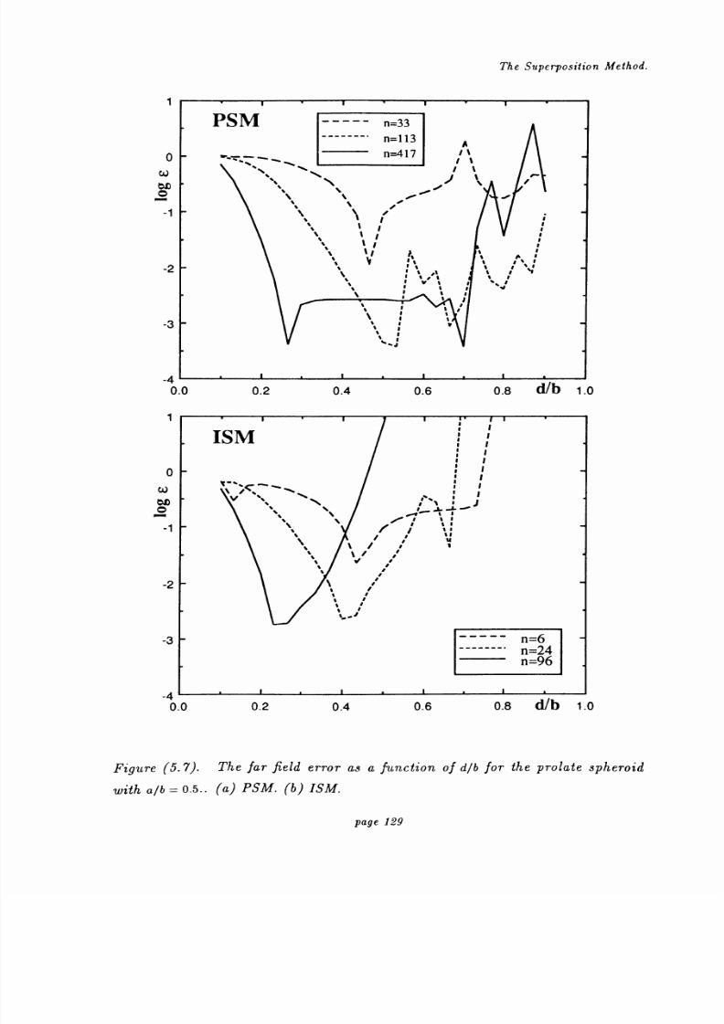
8/13/2019 Richard Jeans 1992 PhD Thesis
http://slidepdf.com/reader/full/richard-jeans-1992-phd-thesis 129/215
The Superposition Method.
PSM
`
-2
-3
-4`-0.0
1
0
-1
-2
-3
-4`-0.0 0.2 0.4 0.6 0.8 d/b 1.0
Figure (5.7). The far field error as a function of d/b for the prolate spheroid
with alb = 0.5.. (a) PSM. (b) ISM.
----- n=33
n=113
n=417
111 i
Y
i
i
1ir
0.2 0.4 0.6 0.8 dlbto
ISM
`/ ..
4
4`d
.
ii
n=6n=24n=96
page 129

8/13/2019 Richard Jeans 1992 PhD Thesis
http://slidepdf.com/reader/full/richard-jeans-1992-phd-thesis 130/215
The Superposition Method.
8
PSM
6
öbD
04
2
0
6
b1DO
4
---- n=33n=113n=417
/
J`
el
0.2 0.4 0.6 0.8 d/b 1.o
ISM
-2 --0.0
8r
n=6n=24n=96
R
r
2
0
0.2 0.4 0.6 0.8 dlb 1.0-2`
0.0
Figure (5.8). The velocity reconstruction error norm as a function of d/b for
the prolate spheroid with a/b = 0.5. (a) PSM. (b) ISM.
page 130

8/13/2019 Richard Jeans 1992 PhD Thesis
http://slidepdf.com/reader/full/richard-jeans-1992-phd-thesis 131/215
Elasto-Acoustic Problem.
CHAP TER 6.
Elasto-Acoustic Problem
6.1 Introduction
Previous chapters have been concerned with the acoustic analysis of rigid submerged struc-
tures. When a submerged structure is elasticly deformed by the acoustic pressure acting on its
surface, the acoustic model needs to be expanded to account for this fluid-structure interaction.
The established technique for modeling the elastic deformation is the Finite Element Method
(FEM). An elasto-acoustic analysis is performed by coupling the BEM to a FEM structural for-
mulation. The resulting equation set can be solved for the structural displacement and surface
pressure in terms of the structural and acoustic excitation. In this chapter the elasto-acoustic
analysis of thin shells will be presented.
6.2 Structural Problem
For an extensive treatment of the FEM the reader is referred to specialized texts, e.g.
Zienkiewicz and Taylor [1989], Hughes [1987], Hinton and Owen [1979]. The following section
is an outline of the thin shell FE11 used in this study. For the thin shell domain, Sl, of density
p, there exists a equilibrium equation relating the applied surface forces, f, the inertial forces
R and the local displacement vector, u,
Cu+R=f, (6.2.1)
where C is the elasticity operator. The FEM is formulated from the minimization of the following
energy functional,
II= 2J
.CUT
(Cu+R-f)) (6.2.2)
The local displacement vector in Eq. (6.2.1) will have six degrees of freedom; three dis-
placement and three rotational components,
page 131
8/13/2019 Richard Jeans 1992 PhD Thesis
http://slidepdf.com/reader/full/richard-jeans-1992-phd-thesis 132/215
Elasto- Acoustic Problem.
uT
uy
u,zu=0.T
eyeZ
It is related to the global displacement vector by means of a transformation matrix,
u=TU,
6.2.3)
6.2.4)
where T is the matrix of directional cosines and U is the displacement vector expressed in the
global coordinate system.
The structural domain is modeled by Mindlin type thin shell elements, defined in three
dimensional space. These elements are derived from a three dimensional continuum element
using a degeneration technique. The degeneration relies on two assumptions; first the normals to
the mid surface of the element remain straight after deformation and second the stress component
normal to the shell is constrained to zero.
The thin shell elements are defined geometrically by the same set of interpolation functions
used in the acoustic boundary element problem. This conformity between the acoustic and
structural meshes simplifies the coupling between the two formulations, however it is believed
that in most cases, refinement of the resulting formulation would be most efficiently achieved
by different acoustic and structural surface meshes.
Using the shapefunctions defined in Chapter 3,
thelocal displacement
vector canbe
in-
terpolated from the element nodal displacements. For the element j, this interpolation can be
written as a matrix relationship,
-71{vj}.6.2.5)
For nine noded elements the shape function matrix N will have dimensions 6x 54 since { UP}
has six components per node. The local displacement vector given by Eq. 6.2.5) represents the
mid plane displacement vector defined at = 0. The through thickness displacement field is
related to the mid surface displacements by,
page 132

8/13/2019 Richard Jeans 1992 PhD Thesis
http://slidepdf.com/reader/full/richard-jeans-1992-phd-thesis 133/215
Elasto-Acoustic Problem.
ýr = ur+zOy,
icy=tcy -SOX
üz = Uz,
(6.2.6)
where the local z variable ranges from-h/2 to h/2, where h is the thickness of the shell.
These equations reflect the assumption of constant through thickness displacement. The strain
displacement differential operator matrix is defined by,
Exa
ax 0 0
Eya
ay ux
Ery - ay ax0 uy (6.2.7)
E12 aZ
0x
fl,
Eyz 0 a aaz ay
Eq. (6.2.7) can be written in terms of the mid plane displacements using Eq. (6.2.6),
ax0 0 0 zäx
Exy
0 ay 0 z ay 0 0 ux
\ä ä o -z
äzä 0 yfxy
E= =
yO
xo ä x
0
y
1 0 (6.2.8)
L
0 0 ä-1 0 0
-txz 0 0 0 0z7yz 0 0 0 0 0
y
The pseudo-strains yaZ and -tiyz in Eq (6.2.8), are defined at this stage to eliminate the nu-
merical difficulties associated with the drilling degree of freedom, 0, that can arise in the final
structural formulation. The structural strains can now be written in terms of the element nodal
displacements,
E=ýBý J L
)
where,
[Bý= AIM.
The operator9 represents the differential matrix operator in Eq. (6.2.8).
The local stress-strain relationship is defined by,
(6.2.9)
(6.2.10)
page 133

8/13/2019 Richard Jeans 1992 PhD Thesis
http://slidepdf.com/reader/full/richard-jeans-1992-phd-thesis 134/215
Elasto-Acoustic Problem.
a= Dc, (6.2.11)
where D, the reduced constitutive equation, enforces the assumption of zero normal stress. This
matrix can be shown to be given by,
1 v 0 0 0 0 0
1 0 0 0 0 0
D1
E
-v2
µ O
µ
0
O
µ
0
0
0
0
0,
0
where,
v= Poisson's ratio,
E= Young's modulus,
1-v
2
(6.2.12)
(6.2.13)
The constant K defines the pseudo-strain / pseudo-stress relationship and takes a small value of
10-4.
The inertial forces in the structural domain are approximated by,
Ps 0 0
0 ps 0
_0-0
p,0 0 0
0 0 0
0 0 0
= -W2[ps]u,
o 0 0 üx0 0 0 uy0 0 0 üZ
0 0 0 9x '
o 0 0 ey
o 0 0 9y
(6.2.14)
and the structural equilibrium relationship can now be defined using the variational principle
shown in Eq. (6.2.2). This results in a structural equation set defined by,
([K]- w2[M]) {U} = {1 }
,
where the stiffness and mass matrices are assembled from the elemental components;
(6.2.15)
page 134

8/13/2019 Richard Jeans 1992 PhD Thesis
http://slidepdf.com/reader/full/richard-jeans-1992-phd-thesis 135/215
Elasto-Acoustic Problem.
[k ]=in
[m ý= in [MTp,[Jdv,
and,
{ F }= j[rs7]T7fdS
(6.2.16)
(6.2.17)
The expression for the applied body forces in Eq. (6.2.17) is integrated over the surface
of the thin shell, S. This assumes that there are no internal body forces due for example
to thermal expansion. The numerical integrations in Eq. (6.2.16-17) are performed by using
Gaussian quadrature and the local-curvilinear relationships derived in Chapter 2.
6.3 Fluid-Structure Interaction Force
When a submerged elastic thin shell is vibrating, the fluid exerts a force on the surface of
the shell. This force is the fluid-structure interaction force, and it serves to couple the elastic
and acoustic formulations. The applied surface force vector in Eq. (6.2.17) consists of two
components; the applied external forces and the fluid structure interaction force,
{F} = {FA}-
{FI}. (6.3.1)
The force F1 acts in the opposite direction to the normal, and the negative sign in Eq. (6.3.1),
shows that work is done on the structure by the fluid. The force Fj is defined in terms of the
pressure difference across the shell, bp,
{Fj} =f[N]n6pds.
(6.3.2)
,
The modified structural equationis
now givenby,
(K- w2Al) {U} + CA {bp} = {FA}
,(6.3.3)
page 135

8/13/2019 Richard Jeans 1992 PhD Thesis
http://slidepdf.com/reader/full/richard-jeans-1992-phd-thesis 136/215
Elasto-Acoustic Problem.
where the area matrix A can be approximated by the same diagonal area matrix defined in Chap-
ter 4. The matrix C represents the transformation of the normal values to the corresponding
normal vectorsin the
global coordinate system,
{FI} = C{FI }, (6.3.4)
where FI is the normal components of the interaction force. For the conforming acoustic and
structural meshes used in this study the coupling matrix C has dimensions nx 6n and is simply
composed of the normal direction cosines. If different structural and acoustic meshes are used
this matrix must accommodate the two sets of interpolation functions.
6.4 Coupled Equation Set
6.4.1 Fluid Filled and Non Closed Shell Problems
The acoustic formulation for the thin shell problem was derived in Chapter 2. This formu-
lation depends on the assumption that the fluid density is equal on both sides of the shell. This
acoustic formulation is valid for non closed thin shells; i.e. shells that do not enclose an interior
volume, and closed thin shells that enclose a volume of fluid with the same density as the fluid
surrounding the shell. This class of problem will be called fluid filled shell problems (FFSP).
The collocation and variational acoustic equation sets are given respectively by,
(6.4.1k{6p} PW2CT{u}än
1
x {bp} = pw2ACT {U} +Al
(6.4.2)
ý
(9n
I
Combining the acoustic equation sets in Eq. (6.4.1) and (6.4.2), with the structural equation
set in Eq. (6.3.3) gives the combined elasto-acoustic equation sets for the collocation and
variational acoustic formulations,
(K- w2M) CA U FA
(6.4.3)CT
-Nk/w2p
bp of
(K- w2M) CA U FA
ACT-Nk/w2p
(ýp)=
(u)(6.4.4)
page 136
8/13/2019 Richard Jeans 1992 PhD Thesis
http://slidepdf.com/reader/full/richard-jeans-1992-phd-thesis 137/215
Elasto-Acoustic Problem.
with,
ap,2UI =an
w p. (6.4.5)
The variational BEM/FEM formulation in Eq. (6.4.4) is symmetric. This is due to the
consistent formulation of the structural and acoustic equation sets. The coupled equation set is
the result of minimizing an energy functional that is symmetric with respect to bp and U. This
functional is given by,
II =2 [{U}T (K - w2M){U} - {bp}T Nk {bp}] + {U}T AC{bp}. (6.4.6)
Eq. (6.4.4) can be derived from the minimization problem,
an=u
Off=O(bp)
(6.4.7)
Thecollocation
BEM/FEM formulation isnon symmetric and cannot
be formulated interms
of a similar variational procedure. Insted it can be thought of as the result of minimizing the
functional in Eq. (6.2.2) subject to a constraint given in Eq. (6.4.1).
6.4.2 Evacuated Closed Shell Problems
The other class of elasto-acoustic problem considered in this study is the evacuated closed
shell problem (ECSP). For this problem the thin shell encloses a domain in which the acoustic
pressure is identically zero. Consequently the pressure difference across the surface of the shell
is simply the exterior surface pressure. The acoustic equation set for the exterior problem is
given in Chapter 3. Neglecting acoustic excitation, the Burton and Miller formulation of the
exterior acoustic problem is given by,
([Mk-
Cpl + aNk) {p+}= W2p
(Lk + a[11ý1k + Cp]) CT {U}. (6.4.8)
The coupled ECSP elasto-acoustic problem is now given by,
(K- w2M) CA U FA
GGG-H/w2p
(np) (u7)(6.4.9)
page 137
8/13/2019 Richard Jeans 1992 PhD Thesis
http://slidepdf.com/reader/full/richard-jeans-1992-phd-thesis 138/215
Elasto-Acoustic Problem.
where the matrices G and H represent the left and right hand side matrices in Eq. 6.4.8) and
ul represents the acoustic excitation for the Burton and Miller problem.
The coupled equation set in Eq 6.4.9) is non symmetric. In previous work this equation set
has been symmetrized by using the energy functional for the acoustic problem Zienkiewicz et al
[1977], Mathews [1979][1986]). This procedure differs from the true variational elasto-acoustic
formulation in that the functional is reconstructed using the non symmetric fluid impedance ma-
trices. The variational elasto-acoustic formulation uses the variational principle as the starting
point for the method.
The formulations in Eqs. 6.4.3) 6.4.4) and 6.4.9) will be referred to as the collocation
coupled method, CCM), the variational coupled method VCM) and the Buton and Miller
coupled method, BMCM). With the correct definitions of G and H, all three formulations may
be generalized by Eq. 6.4.9).
6.5 Solution of Coupled Equation Set
The coupled BEM/FEM equation set may be solved directly. However this is computa-
tionally expensive since it requires the factorization of a 7n x 7n equation set. The normal
procedure is to substitute one equation set into the other. The structure variable methodology,
SVM), involves substituting the fluid equation set into the structural equation set. This method
used by Zienkiewicz et al [1977], results in a fluid modified elastic formulation. The fluid vari-
able methodology involves substituting the structural equation set into the fluid equation set.
Derivation of this method was first given by Wilton [1978] with subsequent work by Mathews
[1979][1986].
6.5.1 Structure Variable Methodology
Neglecting acoustic excitation, the elimination of the fluid variables from Eq. 6.4.9) gives,
K-w2M+w2 pCAH-1GCT) {U} = FA. 6.5.1)
Eq. 6.5.1) is
a matrixequation
of size6n
x6n
and canbe
rewritten
in
a more concise way as,
K- w2[.1I - Mf]) {U} = FA, 6.5.2)
page 138

8/13/2019 Richard Jeans 1992 PhD Thesis
http://slidepdf.com/reader/full/richard-jeans-1992-phd-thesis 139/215
Elasio-Acoustic Problem.
where Alf is the added fluid mass matrix. This is a misleading name since the fluid interaction
actually represents a frequency dependent mass and damping term. The form of this fluid mass
matrix depends on the acoustic formulation;
Alf = pCANk 1CT (CCM), (6.5.3)
_1Il = pCANk -TACT (N,CM), (6.5.4)
Aff = pCAH- GCT (BMCM). (6.5.5)
Only equation (6.5.4) for the fluid stiffness term derived using the variational method is
symmetric, the others are only symmetric in the continuous limit. These terms defined by Eq.
(6.5.3) and (6.5.5) are not exactly symmetric for the following reason presented by Hartmann
[1989].
The generalized collocation acoustic formulation,
He{p} = w2pG{u },
(6.5.6)
expresses the coupling between the surface displacement and pressure distributions, given by a
combination of the SHIE and DSHIE. However the coupling is only satisfied at a finite number
of collocation points. Consequently the interpolated displacements and pressure distributions
are not strictly compatible; i.e. the identity,
lun}T A{PI = iP}T Alu, },
is not satisfied since the matrix identity,
{. V 9}T {1 \*9}H-1G=
[{N9}T {: v9}H-1G]T,
holds only at the collocation points.
(6.5.7)
(6.5.8)
The possibility of symmetrizing the fluid stiffness matrix has been mentioned before. How-
ever Mathews [1979] and Tullberg and Bolteus [1982] find that the highest accuracy is possible
with the unmodified forms of A f given by Eq. (6.5.3) and Eq. (6.5.5).
page 139

8/13/2019 Richard Jeans 1992 PhD Thesis
http://slidepdf.com/reader/full/richard-jeans-1992-phd-thesis 140/215
Elasto-Acoustic Problem.
6.5.2 Fluid Variable Methodology
Eliminating the structural variables from Eq. (6.4.9) gives the modified fluid equation set.
H+GC [K_w2M]-1 CA {bp} =GCT
[K_W2M]-1FA+uj. (6.5.9)
L0 p
This equation set is considerably smaller than the modified structural equation set and it rep-
resents a matrix equation of size nxn. Writing the normal applied force as f and neglecting
acoustic excitation, this equation set can be written in terms of fluid and structural impedance
matrices,
(I + ZfZ3 1) {6p} = ZfZ» 1 n, (6.5.10)
where,
-iwZs 1= CT [K - w2M] -1 CA, (6.5.11)
and,
Zf = -iwNki (CCM), (6.5.12)
Zf= Vk -'A (VCM), (6.5.13)
Zf = -iwH-1G (B-N1CM), (6.5.14)
Only the VCM results in both symmetric fluid and structural impedance matrices.
The fluid variable method is the preferred formulation of the elasto-acoustic problem. The
surface pressure distribution is evaluated using Eq. (6.5.9) and the corresponding displacement
field is found using Eq. (6.3.3). There are two main advantages with this methodology; first the
size of the coupled formulation is significantly smaller than the structural variable formulation
and second for fluid filled thin shell problems the exterior pressure distribution given in Chapter
4, is independent of the displacement. field. The most computationally expensive part in solving
Eq. (6.5.9) is the backward and forward substitution of the structural formulation into the
page 140

8/13/2019 Richard Jeans 1992 PhD Thesis
http://slidepdf.com/reader/full/richard-jeans-1992-phd-thesis 141/215
Elasto-Acoustic Problem.
acoustic formulation. This computational burden can be significantly reduced by reducing the
size of the structural equation set.
6.6 Eigenvector Reduction of the Elastic Formulation
The reduction of the structural equation set can be performed by a variety of transfor-
mations. These include static condensation [Guyan 1965], Lanczos reduction and Eigenvector
reduction. In connection with the elasto-acoustic problem modal reduction is the most estab-
lished technique for reducing the size of the structural equation set. The structural eigenproblem
is defined by,
ýIi- w M]{ek} _0
The eigenvectors, ek, correspond to the n3 non trivial solutions to this equation at the eigenval-
ues, wk. The set of orthogonal eigenvectors, E, are normalized so that the following identities
hold,
ETME = I,(6.6.1)
ET KE= S2,
where the diagonal matrix Q is the set of structural eigenvalues.
Using these identities the inverse of the dynamic stiffness matrix can be written in terms
of a modal summation,
[K- w2M]-i -
By assuming that,
n, fek}fek }T
k=1 k
W «Wm,
it is possible to write,
m[K
- w21\f]-1
T_ n+ {ekl f fk}T2-w2
64)-1 kk=mß-1
k
m<n,
(6.6.2)
(6.6.3)
(6.6.4)
page 141
8/13/2019 Richard Jeans 1992 PhD Thesis
http://slidepdf.com/reader/full/richard-jeans-1992-phd-thesis 142/215
Elasto-Acoustic Problem.
The second summation in Eq. (6.6.4) is a frequency independent static correction term. If m is
large enough then this term can be neglected.
Eq. (6.6.4) can be used in the FVM in order to significantly reduce the computational
burden of the backwards and forwards substitution of the structural equation set into the fluid
formulation. To accurately reconstruct the fluid modified structural response, the number of
`dry' eigenvectors used must be carefully selected. This is not always straight forward since the
structural eigenmodes of a complex structure can be unpredictably modified by the fluid. The
structural inverse impedance in Eq. (6.5.11) can be approximated by,
m{en }{e
IT-2WZs1-ý
ký k (6.6.5)uJ -W2
k=1 k
where
{en}=
CT {ek }. (6.6.6)
Using Eq. (6.6.5) has the added advantage that the individual eigenvectors may be `col-
lapsed' to their normal degrees of freedom only once, insted of at each frequency point.
6.7 Interpolation
Even with careful use of structural symmetry after the calculation of the `dry' eigenmode
solution, a large part of the total computational time needed to calculate the components of
the FVM is taken by the assembly of the acoustic matrices. Benthien [1989] proposed that
the acoustic matrices could be calculated at a reduced number of frequency points and then
interpolated for intermediate points. This interpolation scheme is implemented for the FFSP in
this study.
At wavenumbers greater than one the dominant frequency term of the H matrix is the
exponential term of the Green's free space function. By using the transformation,
hi' (k)_ e-ikhij (k), r=1r1-vu, (6.7.1)
the interpolation scheme is defined by,
page 142

8/13/2019 Richard Jeans 1992 PhD Thesis
http://slidepdf.com/reader/full/richard-jeans-1992-phd-thesis 143/215
Elasto-. 1coustic Problem.
h'ij(k)-
h' (k1) +k-ki
(hij (k2) - h'ij(ki))k2
-kl
(6.7.2)
At low frequencies the fluid matrices can be assumed to be constant. Such interpolation
schemes allow very significant improvements in computation times and recently researchers (eg
Kirkup [1991]) have used interpolation techniques in order to calculate elasto acoustic eigen-
modes.
6.8 Uniqueness and the Coupled Problem
Theproblem of a rigid submerged
thinshell
thatencloses an
interior domaincan
be
con-
sidered as the special case of the general elasto- acoustic problem. The DSHIE acoustic integral
equation for the closed thin shell consists of the equation for the exterior problem and the in-
terior problem. Denoting p- and p+ as the interior and exterior nodal pressure distributions
these equations are,
H{p+} - w2p+G+{'u}= {2ll},
H{p-} - w2p-G-{u} = 0, (6.8.2)
where,
H= Nk and G± =[±i
+ Mk.
(6.8.3)
Thevector u
is thenormal
components of the nodal surface velocity distribution and p± is the
density of the fluid exterior and interior to the thin shell respectively. For the purposes of this
study it is assumed that the interior and exterior waveneumbers are the same; ie the acoustic
speed of sound in both the exterior and interior domains is equal.
The structural equation set for the elasto-acoustic problem can be written as,
S(w){U} + CT A ({p+}-
{p- }) = CA{ f }, (6.8.4)
where the dynamic stiffness matrix is denoted by S(w). The excitation forces and the fluid-
structure interaction forces act on the normal direction degrees of freedom of the structure. It
page 143

8/13/2019 Richard Jeans 1992 PhD Thesis
http://slidepdf.com/reader/full/richard-jeans-1992-phd-thesis 144/215
Elasto-Acoustic Problem.
is advantageous to factorize out the other degrees of freedom. Denoting the normal degrees of
freedom with the subscript n and the others with m, Eq. (6.8.4) can be rewritten as,
Snn Snm un+A0
p+ p-_
(A 0f(6.8.5)
5'mn smm um 0000000
It follows that the structural impedance equation is given by,
Zs{il} + {p+}-
{p-} = ff }, (6.8.6)
where,
-2WZ3 -A-1 [Snn
-SnmSrnmSmn]
.(6.8.7)
The generalized fluid filled thin shell problem is better illustrated by making the following
transformation,
bp=p+-p-,
P=p +P
and,
(6.8.8)
6p=p -p(6.8.9)
p++p .
Using these transformations it is possible to write the coupled formulation as,
Z I0 ü f
-iw[bpMk +2 pI] Nk 0 bp j= eil (6.8.10)
-iw[pMk + 2bpI] 0 Nk ui
Consider the coupled formulation given in Eq. (6.8.10), neglecting for the moment the fluid
variable p,
Z{ } + f6p}= ff}, (6.8.11)
Page 144

8/13/2019 Richard Jeans 1992 PhD Thesis
http://slidepdf.com/reader/full/richard-jeans-1992-phd-thesis 145/215
Elasto-Acoustic Problem.
-ýwSpMk +2 pI {u} + :ýýk{6p}-{ý; }. (6.8.12
At eigenvalues of the interior Neumann problem, both the following homogeneous equations
have non-trivial solutions,
Nk{v} = 0, (6.8.13)
Mk + 2I {v} = 0. (6.8.14)
Assuming that bp # p, then at the interior Neumann eigenvalues Eq. (6.8.12) defines ü uniquely
with respect to the fluid variable bp, but bp is not uniquely defined with respect to the surface
normal velocities, ii, However the structural equation set ,Eq. (6.8.11), uniquely defines both
it,, and 6p, and consequently in the coupled formulation both are defined uniquely at frequencies
corresponding to the Neumann eigenvalues.
When bp = p; ie for the "evacuated" thin shell problem, Eq. (6.8.12) defines neither ufz or
bp uniquely and the coupled formulation no longer has a unique solution. The coupling of the
exterior and interior pressure fields by the structural equation set, ensures that for p- 0 0, the
coupled formulation is unique for all frequencies.
By considering the uncoupled expression for the second fluid variable, p, given in Eq.
(6.8.10), is is possible to see that at the interior Neumann eigenvalues it is not uniquely de-
fined since,
Nk{p} = iwIPMT
+26PI
{Ti} + {ti7}. (6.8.15)
Thus Eq. (6.8.10) is uniquely defined fort and bp but not for p. It is, however, possible to
use a definition of p, derived from the SHIE expressions for the interior and exterior acoustic
problems, that is uniquely defined in terms of p for all frequencies,
21{p} = Mk{bp} - iwSpLk{ü} +pi. (6.8.16)
page 1/5
8/13/2019 Richard Jeans 1992 PhD Thesis
http://slidepdf.com/reader/full/richard-jeans-1992-phd-thesis 146/215
Elasto-. acoustic Problem.
The advantage of this formulation is that it gives p in terms of the other fluid and structural
variables, without the need for matrix factorization.
Consider the specific example of a closed shell containing the same fluid in the exterior and
interior domains. Neglecting acoustic excitation the FVM and SVM elasto-acoustic equation
sets are respectively,
(Z71+Zd 1) {bp} = Zs 1{f}, (6.8.17)
(Zs+Zf){t} ={f}" (6.8.18)
At eigenvalues of the interior Neumann problem the inverse of the fluid impedance matrix is
ill conditioned and the fluid impedance matrix is ill defined. In Eq. (6.8.17) the structure
impedance matrix removes the ill conditioning from the left hand side. Formulated as in Eq.
(6.8.18), the SVM will be ill defined at the critical frequencies. However it can be rewritten as,
(z7'z3+ i) {ü} = Z1{f}. (6.8.19)
It is perhaps computationally unfeasible to formulate the SVM in this way, but it illustrates the
uniqueness of the SVM at the critical frequencies. A similar argument for the evacuated thin
shell fails since both ZI and Zf1 are ill defined at the eigenvalues interior Neumann problem.
In order to obtain a unique solution for the evacuated closed thin shell problem, it is necessary
to use the Burton and Miller formulation of the exterior acoustic problem.
Huang [1984]
proposedthat whilst the evacuated fluid interaction problem was in theory ill
conditioned at internal critical wavenumbers, in practice this is ill conditioning is not seen. His
reasons were that discretization errors remove the degeneracy of the eigenvalues of the H and
G+ matrix in Eq. (6.8.1-2). However the numerical results in this Chapter along with previous
results ('1Mlathews 1986]), show that this proposition is not valid for the high order fluid and
surface interpolation.
Since the elasto-acoustic problem does not break down at the interior Neumann eigenvalues,
as long as p- is non-zero, it is interesting to consider the physical properties of the shell at these
critical wavenumbers. Following the notation of Junger and Feit [1986], modal pressure and
surface velocity are related by,
page 146

8/13/2019 Richard Jeans 1992 PhD Thesis
http://slidepdf.com/reader/full/richard-jeans-1992-phd-thesis 147/215
Elasto-Acoustic Problem.
Wn= fn,
+-nPn-+
2-t-
7-
fn,Zn
n n
_
Zn
Pn = fnZn +4- Zn ,
where,
Z- ip- c_jn(k-a)
(6.8.20)
(6.8.21)
(6.8.22)
(6.8.23)
and the other impedance relationships are defined on page 161 and 233 of Junger and Feit.
For the fluid filled thin shell at the eigenvalues of the interior Neumann problem,
in'(k a) = 0
Assuming p- 00 and c- 00 then the following relationships will hold;
wn=o,
Pn =1,
Pn -- -fn
(6.8.24)
(6.8.25)
(6.8.26)
(6.8.27)
At the interior Neumann eigenvalues the spherical shell will show a rigid response for that
mode, whilst at interior Dirichlet eigenvalues it will display a response independent of the interior
fluid.
6.9 Elastic Thin Plate Problems
The treatment of rigid plate problems has already been introduced in Chapter 4. For the
collocation method,the
pressure
difference distribution is
approximated
in Eq. (4.6.5) by,
HII{5pi}=
{uj}. (6.9.1)
page 147
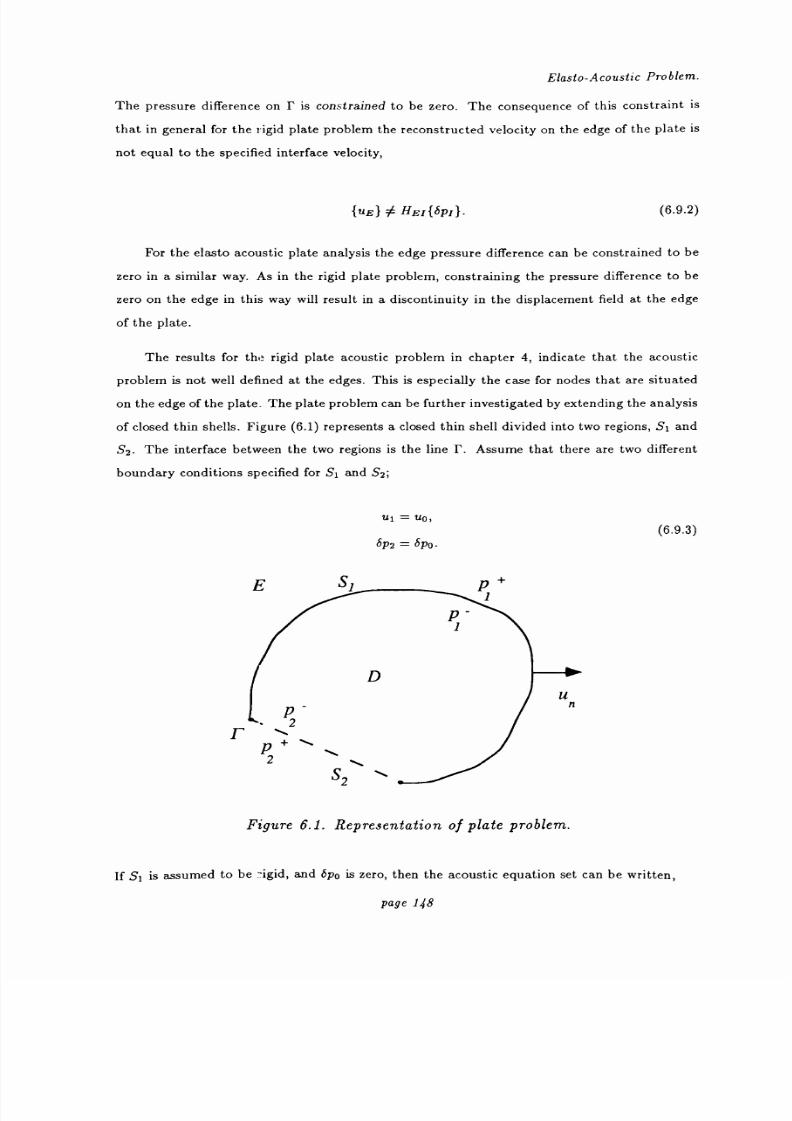
8/13/2019 Richard Jeans 1992 PhD Thesis
http://slidepdf.com/reader/full/richard-jeans-1992-phd-thesis 148/215
Elasto-Acoustic Problem.
The pressure difference on IF is constrained to be zero. The consequence of this constraint is
that in general for the rigid plate problem the reconstructed velocity on the edge of the plate is
not equal to the specified interface velocity,
{UE} 0 HEI{SPI}. 6.9.2)
For the elasto acoustic plate analysis the edge pressure difference can be constrained to be
zero in a similar way. As in the rigid plate problem, constraining the pressure difference to be
zero on the edge in this way will result in a discontinuity in the displacement field at the edge
ofthe
plate.
The results for the rigid plate acoustic problem in chapter 4, indicate that the acoustic
problem is not well defined at the edges. This is especially the case for nodes that are situated
on the edge of the plate. The plate problem can be further investigated by extending the analysis
of closed thin shells. Figure 6.1) represents a closed thin shell divided into two regions, Sl and
S2. The interface between the two regions is the line F. Assume that there are two different
boundary conditions specified for Sl and S2;
U1 = U0,
bp2= bpo.
r
Figure 6.1. Representation of plate problem.
6.9.3)
If Sl is assumed to be -igid, and öpo is zero, then the acoustic equation set can be written,
page 1, 8
F S7 n+

8/13/2019 Richard Jeans 1992 PhD Thesis
http://slidepdf.com/reader/full/richard-jeans-1992-phd-thesis 149/215
Elasto-Acoustic Problem.
Hll H1` bpi
_u° (6.9.4)
H21 H22 0 U2
For the case where r does not contain any surface nodes then this equation may be rear-
ranged to give a solution in terms of the known quantities,
Hip 0 bPi_
uoH21
-1 u2 0(6.9.5)
Continuity of pressure and displacement over IF is satisfied by the interpolation functions.
If howeverthe edge nodes are taken
intoconsideration then
Eq. (6.9.5)results
inan over
determined set of equations for bpl ;
Hll{bpl} = {uo}, (6.9.6)
Hrl{bpl} = {uo}. (6.9.7)
Ignoring Eq. (6.9.7) gives the solution technique given in Eq. (6.9.1). An improvement on this
might be the solution of Eq. (6.9.6) and Eq. (6.9.7) by a least squares method.
6.10 Numerical Results
The elasto-acoustic methodologies were fully implemented in FORTRAN. This was done by
coding the FEM and coupling the resulting matrices into the existing acoustic code. The large
size of the resulting structural matrices and the lack of an out of core solution procedure meant
that only problems of a moderate complexity could be modeled. Ther majority of numerical
results in this chapter correspond to the analysis of submerged elastic spherical shells since
analytical solutions are well established and straight forward. The other problem modeled was
the cantilever plate.
6.10.1 Cantilever Plate
The cantilever plate shown in figure (6.2) was studied with dimensions; a=0.4064, b=
0.2032 and t=0.00267. The plate has constitutive material properties; E=0.2068 x 10¹²,
v=0.3 and p, = 7830. These parameters were chosen so the results could be compared to
those of Coyette and Fyfe [1989]. The rigid wall anchoring the plate at X=0 was incorporated
page 149
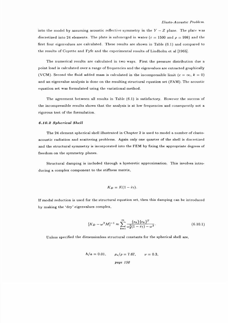
8/13/2019 Richard Jeans 1992 PhD Thesis
http://slidepdf.com/reader/full/richard-jeans-1992-phd-thesis 150/215
Elasto-Acoustic Problem.
into the model by assuming acoustic reflective symmetry in the Y-Z plane. The plate was
discretized into 24 elements. The plate is submerged in water (c = 1500 and p= 998) and the
first four eigenvalues are calculated. These results are shown in Table (6.1) and compared to
the results of Coyette and Fyfe and the experimental results of Lindholm et al [1965].
The numerical results are calculated in two ways. First the pressure distribution due a
point load is calculated over a range of frequencies and the eigenvalues are extracted graphically
(VCM). Second the fluid added mass is calculated in the incompressible limit (c = oo, k= 0)
and an eigenvalue analysis is done on the resulting structural equation set (FAM). The acoustic
equation set was formulated using the variational method.
The agreement between all results in Table (6.1) is satisfactory. However the success of
the incompressible results shows that the analysis is at low frequencies and consequently not a
rigorous test of the formulation.
6.10.2 Spherical Shell
The 24 element spherical shell illustrated in Chapter 2 is used to model a number of elasto-
acoustic radiation and scattering problems. Again only one quarter of the shell is discretized
and the structural symmetry is incorporated into the FEM by fixing the appropriate degrees of
freedom on the symmetry planes.
Structural damping is included through a hysteretic approximation. This involves intro-
ducing a complex component to the stiffness matrix,
KD = K(1 - i-y).
If modal reduction is used for the structural equation set, then this damping can be introduced
by making the `dry eigenvalues complex,
[KD-W
2M]-1 N
r` {ek } {ek }TE
k-wk(1 - 17) - w2
Unless specified thedimensionless
structural constantsfor
the spherical shell are,
h/a = 0.01, p3/p=7.67, v=0.3,
(6.10.1)
page 150

8/13/2019 Richard Jeans 1992 PhD Thesis
http://slidepdf.com/reader/full/richard-jeans-1992-phd-thesis 151/215
Elasto-Acoustic Problem.
cp c = 3.53(1- iy/2), 7=0.01.
The thickness of the shell is denoted h and the structural speed of sound, cp is defined by,
Cp =
Ps(1
E-
v2)
1/2(6.10.2)
Table (6.2) shows a numerical modal analysis of the in vacuo and submerged evacuated
spherical shell compared to the results extracted from Junger and Feit [1986] p282. The eigen-
value results indicate which structural eigenvalue corresponds to the axisymmetric analytical
mode, and the undamped dimensionless frequency is defined by,
SZ = wa/cp. (6.10.3)
An eigenvalue analysis is performed on the `dry' structure to extract the numerical eigen-
values for the 6 and 24 element discretizations. The results show that the numerical `dry'
eigenvalues converge and the agreement with the analytical results is satisfactory. The sub-
merged eigenvalues were evaluated from a graphical frequency plot, to three significant places,
and it was found that there is a slight discrepancy between the coded analytical and Junger and
Feit submerged eigenvalues. Again these results show good accuracy and convergence.
The second set of results showing the ratio of tangential to radial displacement are more
informative. The results for the lower branch modes again show good accuracy for the in vacuo
and submerged ratios, however the numerical calculation of the submerged ratios rapidly looses
accuracy for the higher modes of the upper branch. There are two contributory factors to this
inaccuracy. First there is the inaccuracy of the dry eigenvector and second the inaccuracy of the
fluid modification of the eigenvector. Whilst a refined mesh would reduce the inaccuracy, it may
be more efficient to refine the structural and acoustic problems independently. It is the author's
belief that such a methodology would balance the increased complexity with much improved
efficiency.
Figures (6.3-4) show the pressure gain in the far field from a fluid filled elastic spherical
shell excited by a unit point force. The pressure gain is calculated as the ratio between the far
field pressure and 1pPa For the variational formulation there is high accuracy up to ka = 3.
The contribution to the scattering from the lower branch modes is over approximated, however
the structural damping for the test case is very small. For the collocation method however,
page151

8/13/2019 Richard Jeans 1992 PhD Thesis
http://slidepdf.com/reader/full/richard-jeans-1992-phd-thesis 152/215
Elasto-Acoustic Problem.
there is a similar accuracy in the underlying response, but the excitement of the lower branch
modes is less accurate. After ka ;zzý.5 there should be no contribution to the far field radiation
from the lower branch modes. Although excitation by a point source is a severe test of the
formulation, these results indicate that the consistent formulation of the variational BEM and
FEM may have the edge in accuracy over the coupled collocation BEM/FEM formulation.
The results in figures (6.5-6) show the backscattering form function for the fluid filled
elastic spherical shell. A comparison of the collocation and variational results shows very little
difference in accuracy and close agreement with the analytical result up to ka = 8. The difference
between these results and the radiation results for the point excited spherical shell indicate that
the accuracy of the structural response may be a limiting factor for consistent structural and
fluid meshes. Figure (6.7) shows the back scattered form function for the evacuated thin shell,
calculated using the collocation Burton and Miller formulation.
The behaviour of the coupled SHIE and Burton and Miller formulations applied to the
evacuated spherical shell, at the first Dirichlet critical frequency is shown in figure (6.8).
Figure (6.9) compares the coupled DSHIE and Burton and Miller formulations for the same
problem at the first Neumann critical frequency. Both set of results disprove Huang's conjecture
and show the need for a modified formulation for the evacuated thin shell problem. The
results in figure (6.10) however support the proposal made in this study that for a fluid filled
elastic thin shell, the coupling of the exterior and interior problems by the elastic formulation
removes problems of uniqueness at the critical frequencies. The results of figure (6.10) show
that at the first Neumann frequency the surface pressure difference will be equal to the applied
excitation pressure.
Figures (6.11-14) indicate the advantages of frequency interpolation. The results for the
collocation and variational methods both indicate that a frequency interpolation step of Aka =
1.0 is possible before significant loss in error. Such a frequency interval in these plots represents
the calculation of fluid impedance matrices at approximately 1% of frequency points.
page 152
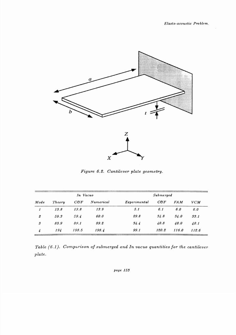
8/13/2019 Richard Jeans 1992 PhD Thesis
http://slidepdf.com/reader/full/richard-jeans-1992-phd-thesis 153/215
Elasto-acoustic Problem.
.A-*o
NL...
_ý
Z
x
Figure 6.2. Cantilever plate geometry.
Mode Theory
In Vacuo
C F Numerical Experimental
Submerged
C F FAM VCM
1 13.8 13.8 13.9 5.1 6.1 6.0 6.0
2 59.3 59..E 60.0 29.8 34.8 34.0 33.1
3 83.9 899.1 89.2 34.4 40.8 40.0 40.1
4 194 198.5 198.4 99.1 120.2 116.0 112.6
Table (6.1). Comparison of submerged and In vacuo quantities for the cantilever
plate.
page 153

8/13/2019 Richard Jeans 1992 PhD Thesis
http://slidepdf.com/reader/full/richard-jeans-1992-phd-thesis 154/215
Elasto-acoustic Problem.
Undamped dimensionless
natural
frequency
Eig e avalue In Vacuo Submerged
Mode n=6 n=24 n=6 n=2.4 J F n=6 n=24 Anal. J F
Lower 1 1 1 0.000 0.000 0.000 0.000 0.000 0.000 0.000
2 2 2 0.713 0.702 0.701 0.322 0.323 0.324 0.318
3 5 5 0.909 0.835 0.830 0.424 0.407 0.407 0.392
4 7 7 1.237 0.896 0.881 0.700 0.467 0.465 0.461
Upper 0 11 25 1.613 1.613 1.610 1.270 1.270 1.270 1.220
1 15 27 1.979 1.975 1.980 1.800 1.800 1.800 1.820
2 19 39 2.733 2.724 2.720 2.290 2.300 2.300 2.550
3 29 51 3.744 3.642 3.640 3.370 3.360 3.360 3.420
4 38 68 4.707 4.614 4.600 4.250 4.390 4.390 4.420
Ratio of tangential to radial displacement
In Vacuo Submerged
Mode n=6 n=24 J F n=6 n=24 J F
Lower 1 1.000 1.000 1.000 1.000 1.000 1.000
2 0.275 0.271 0.270 0.252 0.250 0.250
3 0.117 0.122 0.123 0.107 0.116 0.117
4 0.118 0.069 0.070 0.113 0.067 0.068
Upper 0 0.000 0.000 0.000 0.000 0.000 0.000
1 -3.500 -0.500 -0.500 -0.669 -0.668 -0.646
2 -0.593 -0.616 -0.616 -53.700 -153.0 -1.080
3 -0.608 -0.673 -0.680 -22.400 -77.8.0 -3.280
4 -0.688 -0.679 -0.713 -34.200 -110.0 -5.500
Table (6.2). Comparison of submerged and In vacuo quantities for the evacuated
thin shell.
page 154

8/13/2019 Richard Jeans 1992 PhD Thesis
http://slidepdf.com/reader/full/richard-jeans-1992-phd-thesis 155/215
Elasto-acoustic Problem.
130
120
dB
110
100
90
80
70
ci
Analytical
' Variational
.11 ka 10
Figure (6.3). The ; ar field back radiated pressure from a fluid filled sphere ex-
cited by a point unit force. The sphere is discretized into 24 elements and the
variational thin shell formulation was used to model the acoustic response. The
structural equation set is reduced using 100 eigenvectors.
page 155

8/13/2019 Richard Jeans 1992 PhD Thesis
http://slidepdf.com/reader/full/richard-jeans-1992-phd-thesis 156/215
Elasio-acoustic Problem.
130
120
dB
110
100
90
80
70
r,
F
1
Analytical
° Collocation
1 1 ka 10
Figure (6.4). The far field back radiated pressure from a fluid filled sphere ex-
cited by a point unit force. The sphere is discretized into 24 elements and the
collocation thin shell formulation was used to model the acoustic response. The
structural equation set is reduced using 100 eigenvectors.
page 156
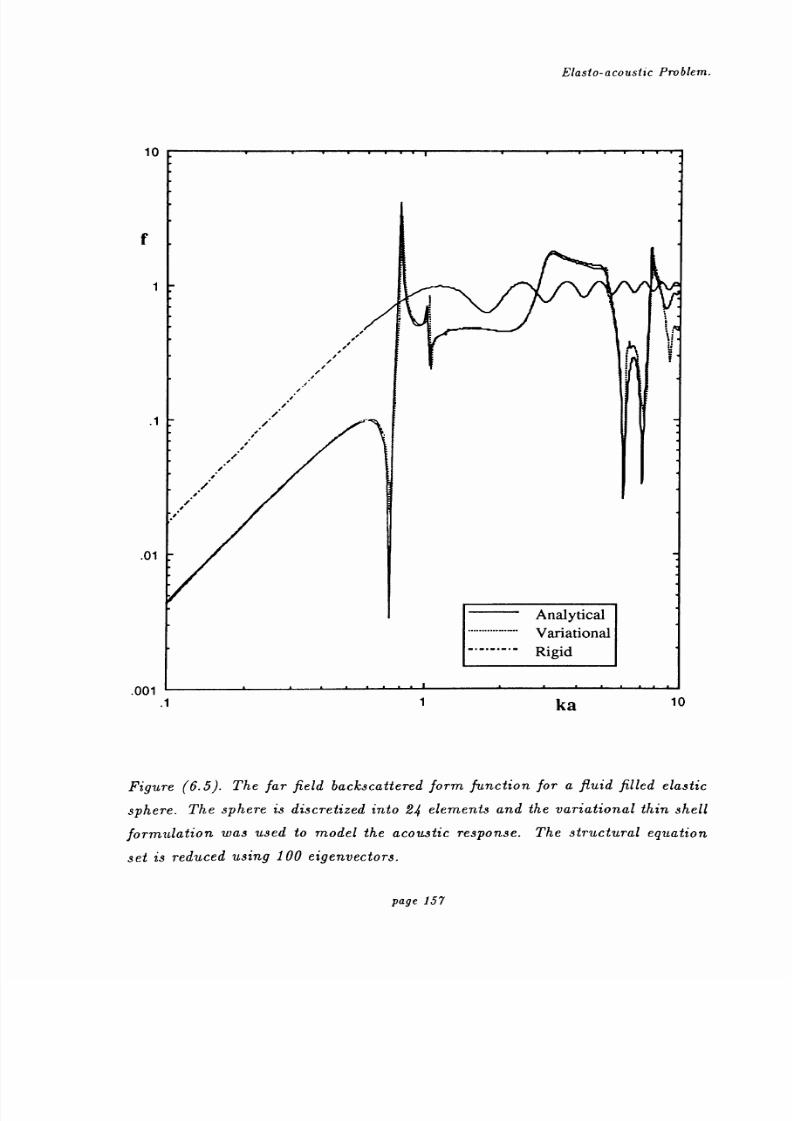
8/13/2019 Richard Jeans 1992 PhD Thesis
http://slidepdf.com/reader/full/richard-jeans-1992-phd-thesis 157/215
Elasto-acoustic Problem.
10
f
1
.1
01
i
/i
/
,ý'
'/
i
i
Analytical
'. '. Variational
Rigid
.0011 1 ka 10
Figure (6.5). The far field baclcscattered form function for a fluid filled elastic
sphere. The sphere is discretized into 24 elements and the variational thin shell
formulation was used to model the acoustic response. The structural equation
set is reduced using 100 eigenvectors.
page 157
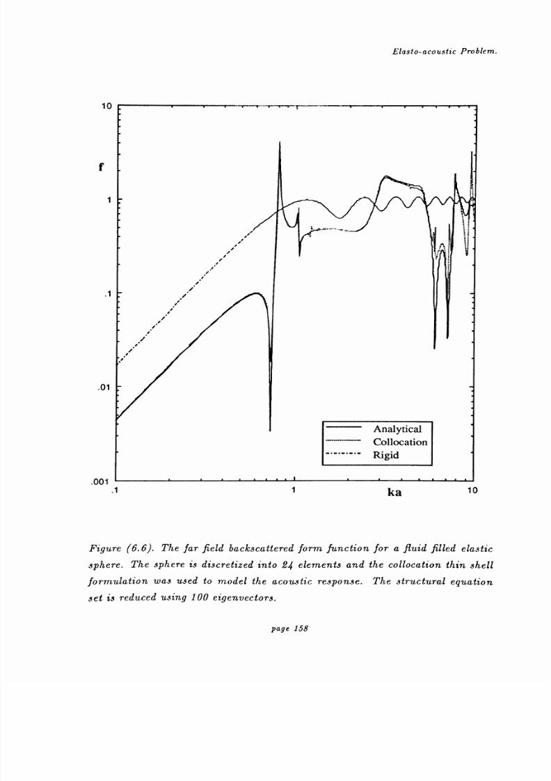
8/13/2019 Richard Jeans 1992 PhD Thesis
http://slidepdf.com/reader/full/richard-jeans-1992-phd-thesis 158/215
Elasto-acoustic Problem.
10
f
1
I
.1
.01
ii
.41
i
.i
Analytical
Collocation
Rigid
.0011 1 ka 10
Figure (6.6). The far field backscattered form function for a fluid filled elastic
sphere. The sphere is discretized into 2.4 elements and the collocation thin shell
formulation was used to model the acoustic response. The structural equation
set is reduced using 100 eigenvectors.
page 158

8/13/2019 Richard Jeans 1992 PhD Thesis
http://slidepdf.com/reader/full/richard-jeans-1992-phd-thesis 159/215
Elasto-acoustic Problem.
10
f
1
1
.01
1' ,,
i
i
i
i
i
ii
1i
i
i
ii
ii
i,
i
.; NX,
Analytical
Numerical
Rigid
1 1 ka 10
Figure (6.7). The far field backscattered form function for an evacuated elastic
sphere. The sphere is discretized into 24 elements and the Burton and Miller
collocation formulation was used to model the acoustic response. The structural
equation set is reduced using 50 Lanczos vectors.
page 159
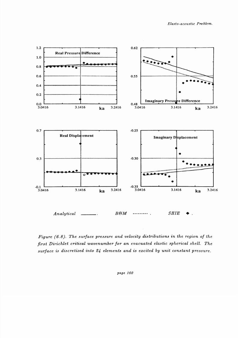
8/13/2019 Richard Jeans 1992 PhD Thesis
http://slidepdf.com/reader/full/richard-jeans-1992-phd-thesis 160/215
Elasto-acoustic Problem.
1.2
1.0
0.8
0.6
0.4
0.2
nn
Real Pressur Difference
"
0.62
I\'
0.55
nAQ. v v. -to
3.0416 3.1416 ka 3.2416 3.0416
0.7
0.3
-0.1L-
3.0416
-0.25
"
"
Imaginary Press e Difference
3.1416 ka 3.2416
Imaginary D splacement
40
-0.30
_nZS
"" ". "tý.. l..
""
"
-V. J
3.1416 ka 3.2416 3.0416
Analytical.
BYM ---------
3.1416 ka 3.2416
SHIE f.
Figure (6.8). The surface pressure and velocity distributions in the region of the
first Dirichlet critical wavenumber for an evacuated elastic spherical shell. The
surface is discretized into 24 elements and is excited by unit constant pressure.
Real Displa cement
"
0
page 160

8/13/2019 Richard Jeans 1992 PhD Thesis
http://slidepdf.com/reader/full/richard-jeans-1992-phd-thesis 161/215
Elasto-acoustic Problem.
1.1
1.0
09
Real Pressur Difference
40--- -------------------
03
0.2
Al
w
-----------------
Imaginary Press e Difference
4.4934 ka 45934.3934 4.4934 ka 45934 4.3934
0.05
0.00
_nnS
Real Disp
4.3934
40
-0.1
-0.2
-0.34.4934 ka 4.5934 43934 4.4934
ka 4.5934
Analytical_.
B&M --------- .DSHIE f.
Figure (6.9). The surface pressure and velocity distributions in the region of the
first Neumann critical wavenumber for an evacuated elastic spherical shell. The
surface is discretized into 24 elements and is excited by unit constant pressure.
Imaginary Dis acement
page 161

8/13/2019 Richard Jeans 1992 PhD Thesis
http://slidepdf.com/reader/full/richard-jeans-1992-phd-thesis 162/215
Elasto-acoustic Problem.
1.03
1.00
Real PrLure
Difference0.001
0.000
0.97 -4.3934
0.03
nnni
Imaginary Press re Difference
0.003
Imaginary Displacement
0.00
Displacement
-v. w i
4.4934 4.5934 4.3934 4.4934 4.5934
-0.03-
4.3934
0.000
-0.0034.4934 4.5934 4.3930 4.4930 4.5930
Analytical Collocation f.
Figure (6.1 D). The surface pressure and velocity distributions in the region of the
first Neumann critical wavenumber for a fluid filled elastic spherical shell. The
surface is discretized into 24 elements and is excited by unit constant pressure.
page 162

8/13/2019 Richard Jeans 1992 PhD Thesis
http://slidepdf.com/reader/full/richard-jeans-1992-phd-thesis 163/215
Elasto-acoustic Problem.
130
dB
110
90
Analytical
. ka=0.1
130
dB
110
70 -
0.1 1.1 ka 2.1
Analytical
Oka=0.2
700. 1.1 ka 2.1
Figure 6.11). The far field back radiated pressure from a fluid filled sphere
excited by a point unit force. The results are calculated using the collocation
method with frequency interpolation at a) Oka = 0.1 and b) Oka = 0.2.
90
page 163

8/13/2019 Richard Jeans 1992 PhD Thesis
http://slidepdf.com/reader/full/richard-jeans-1992-phd-thesis 164/215
Elasto-acoustic Problem.
130
dB
110
90
Analytical
Oka=1.0
130
dB
110
700.1 1.1 ka 2.1
90
..... --°...... Analytical
Aka=-2.0
700.1 1.1 ka 2.1
Figure (6.12). The far field back radiated pressure from a fluid filled sphere
excited by a point unit force. The results are calculated using the collocation
method with frequency interpolation at (a) Oka = 1.0 and (b) Oka = 2.0.
page 164

8/13/2019 Richard Jeans 1992 PhD Thesis
http://slidepdf.com/reader/full/richard-jeans-1992-phd-thesis 165/215
Elasto-acoustic Problem.
130
dB
110
90
............... Analytical
Oka=O.
130
dB
110
700.1 1.1 ka 2.1
90
............... Analytical
Oka-0.2
700.1 1.1 ka 2.1
Figure 6.13). The far field back radiated pressure from a fluid filled sphere
excited by a point unit force. The results are calculated using the variational
method with frequency interpolation at a) Oka = 0.1 and b) Oka = 0.2.
page 165

8/13/2019 Richard Jeans 1992 PhD Thesis
http://slidepdf.com/reader/full/richard-jeans-1992-phd-thesis 166/215
Elasto-acoustic Prvblem.
130
dB
110
90
..... -. .. - Analytical
Oka=1.0
130
dB
110
70
0.1 1.1 ka 2.1
90
. .............. Analytical
Aka=2.0
70 '-
0.1 1.1 ka 2.1
Figure (6.14). The far field back radiated pressure from a fluid filled sphere
excited by a point unit force. The results are calculated using the variational
method with frequency interpolation at (a) Oka = 1.0 and (b) Oka = 2.0.
page 166

8/13/2019 Richard Jeans 1992 PhD Thesis
http://slidepdf.com/reader/full/richard-jeans-1992-phd-thesis 167/215
Lanc: os vectors in elasto-acoustic analysis.
CHAP TER 7.
Lanczos vectors in elasto-acoustic analysis
7.1 Introduction
This chapter evaluates the use of Lanczos vectors in the coupled Boundary Element Method
and Finite Element Method with a view to improving the currently available solution techniques,
for exterior field problems, in terms of computational speed and accuracy. It has been shown
that the fluid variable method is the most economical solution technique for these exterior
field problems. In the fluid variable method, the structural equation set is substituted into the
acoustic equation set, the structural displacement vector is subsequently eliminated and solution
of the resultant matrix equation set yields the normal surface pressure. The disadvantage of
solving the coupled system in this manner is that considerable computational effort is expended
in a forward and backward substitution of the dynamic structural matrix into the acoustic
equation set. Therefore it is advantageous to use a reduced basis technique to represent the
dynamic structural matrix, in order to reduce the computational burden of this forward and
backsubstitution process, required at each
frequency.
In Chapter 6 an eigenvector reduction of the dynamic structural matrix was used in order
to ease this computational burden. The difficulty in using the modal approach, is the large num-
ber of eigenvectors required to accurately represent the dynamic response of the `dry structure.
Recent work (Nour-Omid and Clough [1984], Chen and Taylor [1989] and Nour-Omid and Regel-
brugge [1989]) on the application of Lanczos vectors to the solution of interior fluid-structure
interaction problems has shown far fewer Lanczos vectors are required to represent the dynamic
structural matrix. The increased accuracy of these vectors is due in part to the manner in which
the loading vector is incorporated into their generation; the starting vector for the Lanczos al-
gorithm, as will be demonstrated later in the chapter, is the dynamic deflection shape. Not only
are far fewer Lanczos vectors required to accurately represent the submerged elastic structure,
these vectors are also, computationally less expensive to generate than eigenvectors.
In this chapter two different methods for which the application of Lanczos vectors are used
to solve the coupled fluid-structure interaction problem will be presented. First the solution of
the exterior acoustic problem for evacuated closed thin elastic shells is studied. The collocation
method is used and to ensure that the acoustic formulation is valid throughout the entire fre-
quency range, the methodology of Burton and Miller is implemented. The finite element model
page 167

8/13/2019 Richard Jeans 1992 PhD Thesis
http://slidepdf.com/reader/full/richard-jeans-1992-phd-thesis 168/215

8/13/2019 Richard Jeans 1992 PhD Thesis
http://slidepdf.com/reader/full/richard-jeans-1992-phd-thesis 169/215
Lanc: os rectors in elasto-acoustic analysis.
KQ=K-a2M. (7.2.3)
This spectral shift improves the Lanczos representation of the structural equation set by forcing
the starting vector to be a more appropriate dynamic displacement shape.
It can be shown (Nour-Omid and Clough [1984], Chen and Taylor [1989] and Nour-Omid
and Regelbrugge [1989]) that the algorithm for generating successive Lanczos vectors is given
by,
ro = Kam FA, (7.2.4)
qo = 0, (7.2.5)
,Qj _
ýrý11L1rý-i)1ý2.
(7.2.6)
rj-1qj = a
(7.2.7)
rj = Kv Mqj, (7.2.8)
aj = qý MTA, (7.2.9)
ri = ri - aj qj -3jgj-i, (7.2.10)
where the set of m Lanczos vectors are defined by,
m
Qm = qi. (7.2.11)
Using this set of Lanczos vectors it is now possible to reduce the dynamic structural equa-
tion. By writing,
1u} = Q,n x}. (7.2.12)
and premultiplying Eq. (7.2.1) by QmMKý 1, the transformed dynamic structural equation is
given by,
page 169

8/13/2019 Richard Jeans 1992 PhD Thesis
http://slidepdf.com/reader/full/richard-jeans-1992-phd-thesis 170/215
Lancxos vectors in elasto-acoustic analysis.
[(Qm1ý1(wm ý2QmMKo MQm)-w2Q MAC-1,11Q,
n]{x} = Qm-ý1KQ1 F }. (7.2.13)
From the orthogonal properties of the Lanczos vectors, Eq. (7.2.13) can be greatly simpli-
fled. The left hand side can be transformed by noting that,
QmMK; 1MQ,n = Tm, (7.2.14)
QT= Im, (7.2.15)
where the tri-diagonal matrix Tm is defined by,
a1 /32
32 az 03
TI. (7.2.16)
Qm-1 am-1 Qm
Qm am
The right hand side of Eq. (7.2.13) is given simply by,
QT MKS 1{FA}= {9,,, , (7.2.17)
where, if el is defined as the first column of the identity matrix Im, g,,, is given by,
{g,,, } = ßi{el}. (7.2.18)
Finally the reduced dynamic structural equation can be written as,
[im + (0,2- w2) Tm] {x} _ {g,,,}. (7.2.19)
There are several numerical points that need to be considered before numerically imple-
menting a Lanczos algorithm. Although in theory the orthogonalization of each Lanczos vector
page 170
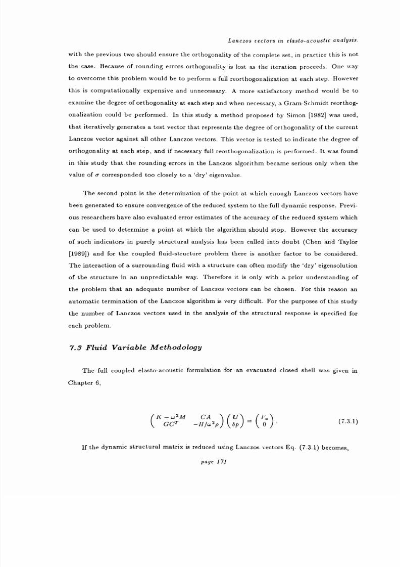
8/13/2019 Richard Jeans 1992 PhD Thesis
http://slidepdf.com/reader/full/richard-jeans-1992-phd-thesis 171/215
Lanczos rectors in elasto-acoustic analysis.
with the previous two should ensure the orthogonality of the complete set, in practice this is not
the case. Because of rounding errors orthogonality is lost as the iteration proceeds. One way
to overcome this problem would be to performa
full
reorthogonalization at each step.
However
this is computationally expensive and unnecessary. A more satisfactory method would be to
examine the degree of orthogonality at each step and when necessary, a Gram-Schmidt reorthog-
onalization could be performed. In this study a method proposed by Simon [1982] was used,
that iteratively generates a test vector that represents the degree of orthogonality of the current
Lanczos vector against all other Lanczos vectors. This vector is tested to indicate the degree of
orthogonality at each step, and if necessary full reorthogonalization is performed. It was found
in thisstudy
that therounding errors
in the Lanczosalgorithm
becameserious only when
the
value of o corresponded too closely to a `dry eigenvalue.
The second point is the determination of the point at which enough Lanczos vectors have
been generated to ensure convergence of the reduced system to the full dynamic response. Previ-
ous researchers have also evaluated error estimates of the accuracy of the reduced system which
can be used to determine a point at which the algorithm should stop. However the accuracy
of such indicators in purely structural analysis has been called into doubt (Chen and Taylor
[1989]) and for the coupled fluid-structure problem there is another factor to be considered.
The interaction of a surrounding fluid with a structure can often modify the `dry eigensolution
of the structure in an unpredictable way. Therefore it is only with a prior understanding of
the problem that an adequate number of Lanczos vectors can be chosen. For this reason an
automatic termination of the Lanczos algorithm is very difficult. For the purposes of this study
the number of Lanczos vectors used in the analysis of the structural response is specified for
each problem.
7.3 Fluid Variable Methodology
The full coupled elasto-acoustic formulation for an evacuated closed shell was given in
Chapter 6,
7K- w2M CA
(U)
_ FaG
-H/w2pbp -0
(7.3.1)
If the dynamic structural matrix is reduced using Lanczos vectors Eq. (7.3.1) becomes,
page 171

8/13/2019 Richard Jeans 1992 PhD Thesis
http://slidepdf.com/reader/full/richard-jeans-1992-phd-thesis 172/215
Lanczos vectors in elasto-acoustic analysis.
(In+(o2_w2)Tm Qm111 'ý 1CA x gmGCTQm
-H/w2p
bp -0(7.3.2)
Following the fluid variable methodology the `participation' factors x are eliminated and
the fluid-structure interaction equation is given by,
wH p+
GCQm [I, + 0-2 - w2) Tm] -1QT %I K47-1CT A {bp}=
GCQr [I,, + (cr2
_W2)
T"]- I{9m}.(7.3.3)
Defining,
CQm = Om, (7.3.4)
Qm-11Ko1CT=
[CKo 1MQm]T- O'm (7.3.5)
[Im + (0.2 - w2) Tmý (7.3.6)
Eq. (7.3.3) can be written more concisely as,
H+GemS-1® A {bp} = GO,, S-'{9m}. (7.3.7)
7.4 Added Fluid Mass Methodology
In Chapter 6 the elasto-acoustic problem for an fluid filled or open thin shell was derived
in terms of a fluid added mass term,
(K- w2 [M
- Mf(w)]) {U} = {Fa}, (7.4.1)
where by formulating the acoustic problem in terms of the variational method, ßllis the com-
plex, symmetric and frequency dependent `fluid mass' matrix,
page 172
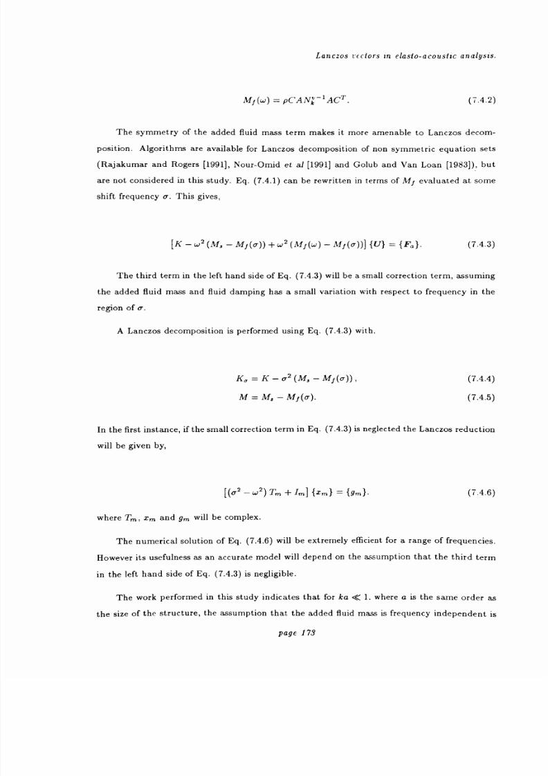
8/13/2019 Richard Jeans 1992 PhD Thesis
http://slidepdf.com/reader/full/richard-jeans-1992-phd-thesis 173/215
Lanczos rectors in elasto-acoustic analysis.
Mf(w) = pCANk-1 ACT (7.4.2)
The symmetry of the added fluid mass term makes it more amenable to Lanczos decom-
position. Algorithms are available for Lanczos decomposition of non symmetric equation sets
(Rajakumar and Rogers [1991], Nour-Omid et al [1991] and Golub and Van Loan [1983]), but
are not considered in this study. Eq. (7.4.1) can be rewritten in terms of Mf evaluated at some
shift frequency o. This gives,
[K- w2 (Ms
- Mf (o)) + w2 (Mf (w) - Mf (o))] {U} = {Fa }. (7.4.3)
The third term in the left hand side of Eq. (7.4.3) will be a small correction term, assuming
the added fluid mass and fluid damping has a small variation with respect to frequency in the
region of a.
A Lanczos decomposition is performed using Eq. (7.4.3) with,
Ka =K-cT2(M8-M1(u)),
M=ms -Mf(Q).
(7.4.4)
(7.4.5)
In the first instance, if the small correction term in Eq. (7.4.3) is neglected the Lanczos reduction
will be given by,
[(0,2_w2)Tm + Im] {Xm1
= t9m}(7.4.6)
where T,,,, x,,, and g,,, will be complex.
The numerical solution of Eq. (7.4.6) will be extremely efficient for a range of frequencies.
However its usefulness as an accurate model will depend on the assumption that the third term
in the left hand side of Eq. (7.4.3) is negligible.
The work performed in this study indicates that for ka « 1. where a is the same order as
the size of the structure, the assumption that the added fluid mass is frequency independent is
page 173

8/13/2019 Richard Jeans 1992 PhD Thesis
http://slidepdf.com/reader/full/richard-jeans-1992-phd-thesis 174/215
Lanczos vectors in elasto-acoustic analysis.
valid and leads to little loss in accuracy. However, for ka -- 1 and ka >1 it will be shown that
this assumption is inadequate.
7.5 Results
To test the different methodologies the spherical shell described in Chapter 6 was used. Hys-
teretic damping was implemented numerically by modifying the stiffness matrix before Lanczos
decomposition.
Figures (7.1-4) show the results of the fluid variable methodology applied to different dis-
cretizations withdifferent
numbers of Lanczos vectors to characterize the `dry' structural re-
sponse. The nodal normal velocities were normalized firstly by P(cosO) and then further nor-
malized with the formula,
1Olog12
Ivn(n + 1)I2exact
(7.5.1)
The modal analytical solution was taken from the work by Geers and Felippa [1983] and
corresponds to the solutions obtained for a submerged, lightly damped, vibrating elastic sphere
excited by loads that are functions of the Legendre polynomial.
The results in figures (7.1-4) show that only 5 Lanczos vectors are needed to accurately
represent the dynamic deflection of the structure. For more complicated shell geometries care
needs to be shown in choosing the number of Lanczos vectors in order not to exclude higher
structural modes that may be significantly perturbed by the influence of the fluid interaction.
Tables (7.1-2) show in more detail the degree of accuracy of the results shown in figures (7.1-4).
The solutions for the higher modes would converge with the use of a finer mesh.
Figures (7.5-8) show the results of an eigenvector decomposition of the dynamic structural
matrices. These results also show good accuracy and convergence, however a higher number of
eigenvectors are needed than Lanczos vectors for convergence. Figure 7 shows the absence of a
structural resonance with 50 eigenvectors, a resonance that is accurately reproduced with only
5 Lanczos vectors.
The added mass formulation was tested in the far field region only, with the fluid mass
correction being evaluated at the lowest frequency. The same structural constants were used
page 17!
8/13/2019 Richard Jeans 1992 PhD Thesis
http://slidepdf.com/reader/full/richard-jeans-1992-phd-thesis 175/215
Lanczos rectors in elasio-acoustic analysis.
for the fluid filled shell as previously. The acoustic speed of sound in water was assumed to
be 1500m/s. Figure 7.9) shows the results for the far-field pressure radiated at 9=0 by a
fluid filled sphere excited by a point force at 0=0. The pressure is measured in dB using one
micropascal at one metre as the reference level. The exact analytical series solution is given on
the same figure.
It was shown in Chapter 6 that the elasto-acoustic problem for fluid filled or open shells is in
general well defined at all frequencies. However, for fluid filled shells, the added fluid mass will
will not be well defined at the eigenvalues of the interior Neumann problem. This problem can
be circumvented by calculating the added fluid mass term away from these critical frequencies.
It may be observed from Figure 9 that for low frequencies, that is ka «1 the agreement
with the analytical solution is excellent. The difference between using 10 or 40 Lanczos vectors
is very small, indicating that the solution converges for a small number of Lanczos vectors.
However as the frequency increases the converged numerical solution displays a loss in accuracy
in comparison to the analytical solution. This loss in accuracy was expected in this frequency
regime as the third term on the right hand side in Eq. 7.4.3) is no longer negligible at these
higher frequencies. For this methodology to be effective at these higher frequencies, high order
frequency terms would need tobe
added to the formulation.
It was thought that use of the Lanczos methodology would be particularly beneficial for
scattering problems. The reduction of the dynamic structural matrix is performed in terms of
the incident acoustic wave and FA in equation 7.2.4) is defined by,
{FA}=ACT{p}
where p; is the incident pressure.
7.5.2)
Figure 7.10) shows the results for the far field back scattering of a plane wave by an
evacuated spherical shell with the same parameter values as used for the radiation problems.
One quarter of a sphere was discretized into 24,9-noded elements. The results, calculated
using the fluid-variable methodology, are presented as a plot of form function, a commonly
used scattering measure, against wavenumber. Twenty Lanczos vectors were used to model the
elastic structural response. The results obtained are compared to an analytical series solution
given by Junger and Feit [1986], for two different values of structural loss factor. Higher solution
accuracy was attained with increased structural damping. It appears therefore, that considerable
accuracy, is needed in the determination of the structural elastic response.
page175
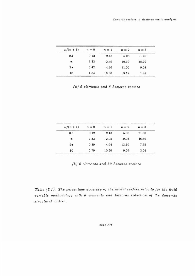
8/13/2019 Richard Jeans 1992 PhD Thesis
http://slidepdf.com/reader/full/richard-jeans-1992-phd-thesis 176/215
Lanczos vectors in elasto-acoustic analysis.
w/ nß-1) n=0 n=1 n=2 n=3
0.1 0.12 2.13 5.06 21.30
7r 1.33 2.49 10.10 48.70
2ir 0.42 4.96 11.00 9.08
10 1.64 18.30 9.12 1.88
a) 6 elements and 5 Lanczos vectors
w/ n+1) n=0 n=1 n=2 n=3
0.1 0.12 2.13 5.06 21.30
7r 1.33 2.95 9.05 46.40
2ir 0.39 4.94 13.10 7.65
10 0.79 10.50 9.09 2.04
b) 6 elements and 20 Lanczos vectors
Table 7.1). The percentage accuracy of the modal surface velocity for the fluid
variable methodology with 6 elements and Lanczos reduction of the dynamic
structuralmatrix.
page 176

8/13/2019 Richard Jeans 1992 PhD Thesis
http://slidepdf.com/reader/full/richard-jeans-1992-phd-thesis 177/215
Lanczos vectors in elasto-acoustic analysts.
w/ n+1) n=0 n=1 n=2 n=3
0.1 0.01 0.20 0.30 1.46
ir 1.56 2.31 6.38 21.90
2ir 0.72 0.21 0.91 1.96
10 0.32 0.97 10.00 0.26
a) 24 elements and 5 Lanczos vectors
w/ n+1) n=0 n=1 n=2 n=3
0.1 0.01 0.20 0.30 1.46
7r 1.56 2.34 6.46 24.60
2ir 0.73 0.20 0.73 1.15
10 0.31 1.03 9.50 0.98
b) 24 elements and 20 Lanczos vectors
Table 7.2). The percentage accuracy of the modal surface velocity for the fluid
variable methodology with 24 elements and Lanczos reduction of the dynamic
structuralmatrix.
page 177
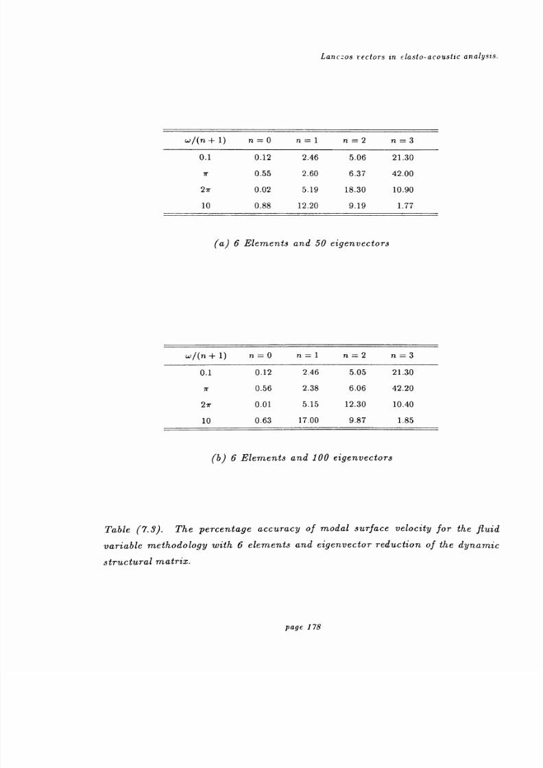
8/13/2019 Richard Jeans 1992 PhD Thesis
http://slidepdf.com/reader/full/richard-jeans-1992-phd-thesis 178/215
Lanczos rectors in elasto-acoustic analysis.
w/ n+1) n =0 n=1 n=2 n=3
0.1 0.12 2.46 5.06 21.30
T 0.55 2.60 6.37 42.00
27r 0.02 5.19 18.30 10.90
10 0.88 12.20 9.19 1.77
a) 6 Elements and 50 eigenvectors
w/ n+1) n=0 n=1 n=2 n=3
0.1 0.12 2.46 5.05 21.30
7r 0.56 2.38 6.06 42.20
2ir 0.01 5.15 12.30 10.40
10 0.63 17.00 9.87 1.85
b) 6 Elements and 100 eigenvectors
Table 7.3). The percentage accuracy of modal surface velocity for the fluid
variable methodology with 6 elements and eigenvector reduction of the dynamic
structural matrix.
page 178

8/13/2019 Richard Jeans 1992 PhD Thesis
http://slidepdf.com/reader/full/richard-jeans-1992-phd-thesis 179/215
Lanc: os vectors in elasto-acoustic analysis.
w/ n+1) n=0 n=1 n=2 n=3
0.1 0.01 0.52 0.29 2.43
7r 0.79 1.20 3.49 37.40
21r 0.35 0.06 0.87 17.20
10 0.14 0.93 10.30 16.10
a) 24 Elements and 50 eigenvectors
w/ n+1) n=0 n=1 n=2 n=3
0.1 0.01 0.52 0.29 1.45
T 0.79 1.20 3.44 15.40
2ir 0.35 0.05 0.86 1.92
10 0.14 0.93 10.10 0.76
b) 24 Elements and 100 eigenvectors
Table 7.4). The percentage accuracy of modal surface velocity for the fluid
variable methodology with 24 elements and eigenvector reduction of the dynamic
structuralmatrix.
page 179

8/13/2019 Richard Jeans 1992 PhD Thesis
http://slidepdf.com/reader/full/richard-jeans-1992-phd-thesis 180/215
Lanczos vectors in elasto-acoustic analysis.
10
dB
-10
-30
.1
30
20
10
dB
0
-10
In
n=
1
20
0
dB
-20
i stU_40
L
10 10.1
n=
40
1
n=
20
dB
0
-'. v
.11 (0/3 10
.20L
.11 U4 10
Figure (7.1). Velocity response for n=0,1,2 and 3 excitation of a submerged
spherical shell discretised into 6 elements using the fluid variable methodology
and 5 Lanczos vectors. w is the dimensionless frequency w/c. The velocities are
normalised with respect to v(n + 1)exact.
62 10
page 180
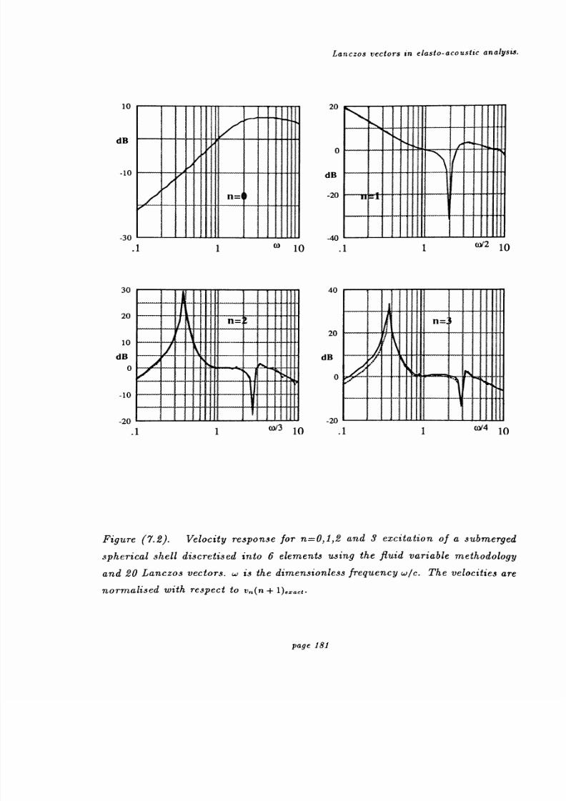
8/13/2019 Richard Jeans 1992 PhD Thesis
http://slidepdf.com/reader/full/richard-jeans-1992-phd-thesis 181/215
Lanczos vectors in elasto-acoustic analysis.
10
dB
-10
-30 L
.1
30
20
10
dB
0
-10
In
n.
1
20
0
dB
-20
fiL2i1-40
10 `
w 10.1
1
n=
40
20
dB
0
-w
.11
n=
Yii[C
H2O
`
wý3 10(r
.11 w/4 10
Figure (7.2). Velocity response for n=0,1,2 and 3 excitation of a submerged
spherical shell discretised into 6 elements using the fluid variable methodology
and 20 Lanczos vectors. w is the dimensionless frequency w/c. The velocities are
normalised with respect to v(n + 1)exact.
62 10
page 181

8/13/2019 Richard Jeans 1992 PhD Thesis
http://slidepdf.com/reader/full/richard-jeans-1992-phd-thesis 182/215
Lanczos vectors in elasto-acoustic analysis.
10
dB
-10
-30L
.1
30
20
10
dB
0
-10
-20
.l1 W3 10
-20 L
.11 oY4 10
Figure (7.3). Velocity response for n=0,1,2 and 3 excitation of a submerged
spherical shell discretised into 24 elements using the fluid variable methodology
and 5 Lanczos vectors. w is the dimensionless frequency w/c. The velocities are
normalised with respect to v(n + 1)exnct
n=
1
20
0
dB
-20
ee ssss , in
w 10
-VtJ.
1
n=
40
1 o/2 10
n=20
dB
0
page 182
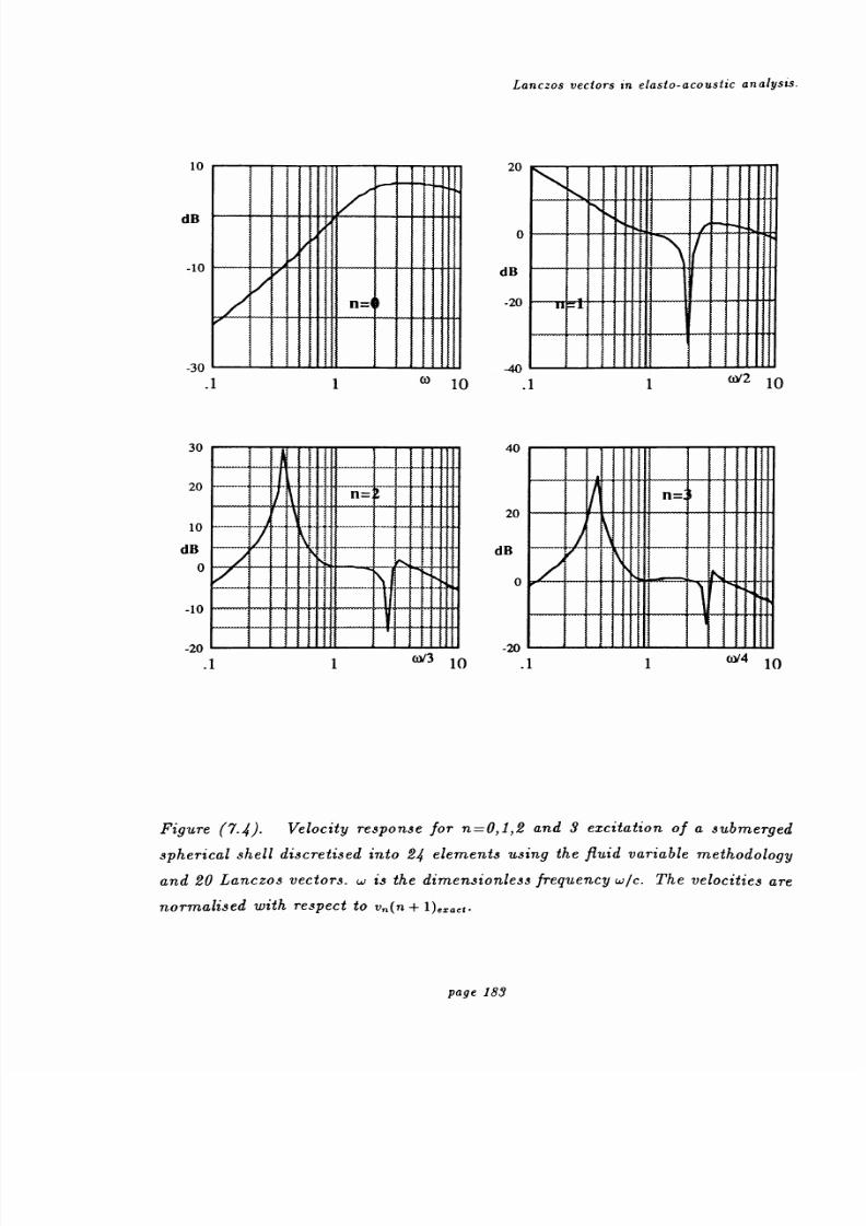
8/13/2019 Richard Jeans 1992 PhD Thesis
http://slidepdf.com/reader/full/richard-jeans-1992-phd-thesis 183/215
Lanczos vectors in elasto-acoustic analysis.
10
dB
-10
-30
.l
30
20
10
dB
0
-10
In
n=
20
0
dB
-20
1 10 10.11
/2 10
n=
-w
.l
40
20
dB
0
i 4. [ L
-If(ý
lii[] [) CL44[]SLYi[1
1 °3 10 oY4 10
Figure (7.4). Velocity response for n=0,1,2 and 3 excitation of a submerged
spherical shell discretised into 24 elements using the fluid variable methodology
and 20 Lanczos vectors. w is the dimensionless frequency w/c. The velocities are
normalised with respect to v(n + 1)esact"
n.
page 183

8/13/2019 Richard Jeans 1992 PhD Thesis
http://slidepdf.com/reader/full/richard-jeans-1992-phd-thesis 184/215
Lanczos vectors in elasto-acoustic analysis.
10
dB
-10
-30
.1
40
20
dB
0
-20L
.1
n=
40
20
dB
0
scisa cttý
1
-20Fscsss 14 gcsss aii
co/3 10.11
oY4 10
Figure (7.5). Velocity response for n=0,1,2 and 3 excitation of a submerged
spherical shell discretised into 6 elements using the fluid variable methodology
and 50 eigenvectors. w is the dimensionless frequency w/c. The velocities are
normalised with respect to v(n + 1)ezact"
n=
20
0
dB
-20
'41ýA0l"l[[
1 co 10.11
c&2 10
n=
page 184

8/13/2019 Richard Jeans 1992 PhD Thesis
http://slidepdf.com/reader/full/richard-jeans-1992-phd-thesis 185/215
Lanczos vectors in elasto-acoustic analysis.
10
dB
-10
-30L
.1
40
20
dB
0
-20L
.1
n=
40
20
dB
0
1 °3 10
20
.11U4 10
Figure (7.6). Velocity response for n=0,1,2 and 3 excitation of a submerged
spherical shell discretised into 6 elements using the fluid variable methodology
and 100 eigenvectors. w is the dimensionless frequency w/c. The velocities are
normalised with respect to v(n + 1)eract.
n=
20
0
dB
-20nil
[[]fL i i
-40
l ]lLC Ot
1w 10.11
(o/2 10
n=
page 185
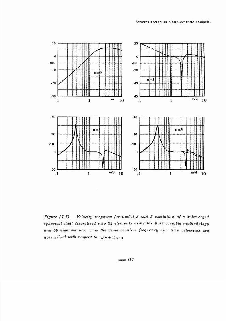
8/13/2019 Richard Jeans 1992 PhD Thesis
http://slidepdf.com/reader/full/richard-jeans-1992-phd-thesis 186/215
Lanczos vectors in elasto-acoustic analysis.
10
0
dB
-10
-20
_'n
n=
.1110 10
.11OY2 10
40
20
dB
0
n-
zu
0
dB
-20
-40
f.n
40
1
-20L
.1
20
dB
0
IA
n-
13 10.11
aY4 10
Figure (7.7). Velocity response for n=0,1,2 and 3 excitation of a submerged
spherical shell discretised into 24 elements using the fluid variable methodology
and 50 eigenvectors. w is the dimensionless frequency w/c. The velocities are
normalised with respect to v (n + 1)exact
page 186

8/13/2019 Richard Jeans 1992 PhD Thesis
http://slidepdf.com/reader/full/richard-jeans-1992-phd-thesis 187/215
Lanczos vectors in elasto-acoustic analysis.
10
dB
-10
-30
.1
40
n: 0
zu
0
dB
-20
-40
Kn
nil
n: 2
20
dB
0
-20L
.1
40
20
dB
0
LL t-7Ffi2I2Flit[72fLGi2L7SSi3t1
1
------ -20
w/3 10.11
oY4 10
Figure (7.8). Velocity response for n=0,1,2 and 3 excitation of a submerged
spherical shell discretised into 24 elements using the fluid variable methodology
and 100 eigenvectors. w is the dimensionless frequency w/c. The velocities are
normalised with respect to v(n + 1)exact"
1 10 10Ti
1 o'2 10
page 187
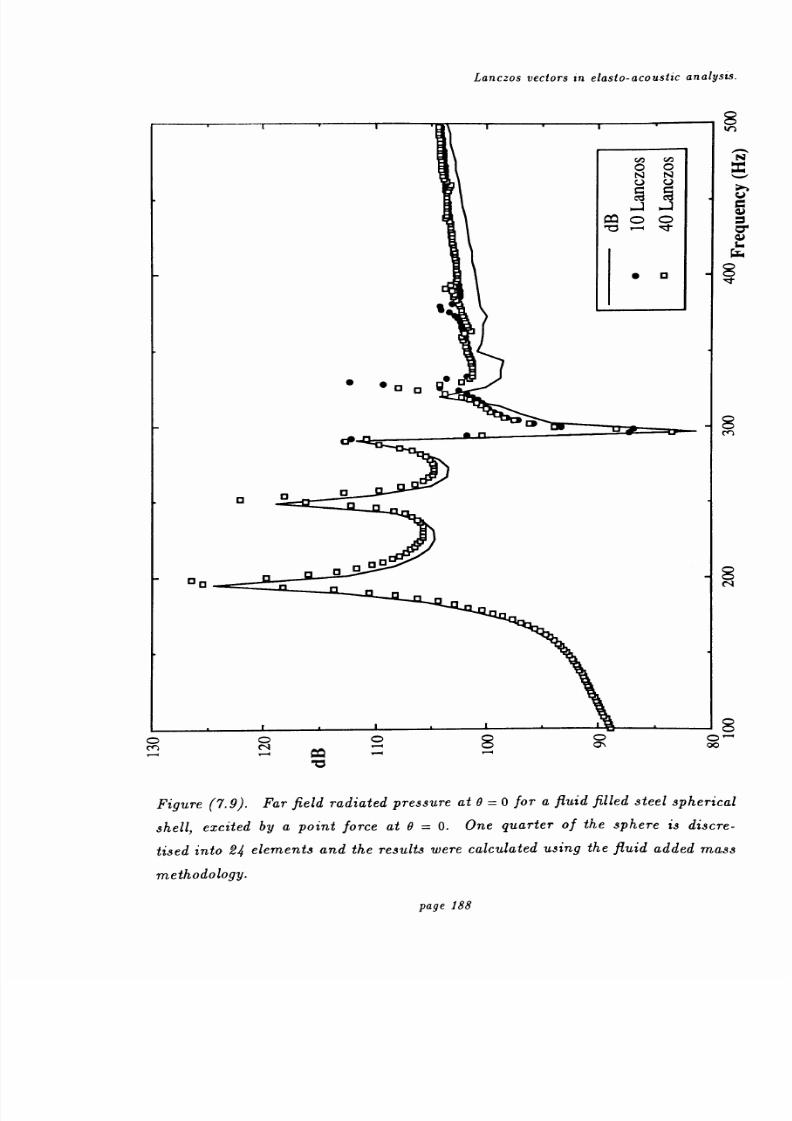
8/13/2019 Richard Jeans 1992 PhD Thesis
http://slidepdf.com/reader/full/richard-jeans-1992-phd-thesis 188/215
Lanczos vectors in elasto-acoustic analysis.
ööÜÜ
bOO
o
oa
CIO
Q0o
o°°
00a
8
V
L
8
8
8
8OOOO0 O, 00ý4
v--4 -d'Lý
Figure (7.9). Far field radiated pressure at 0=0 for a fluid filled steel spherical
shell, excited by a point force at 0=0. One quarter of the sphere is discre-
tised into 24 elements and the results were calculated using the fluid added mass
methodology.
page 188

8/13/2019 Richard Jeans 1992 PhD Thesis
http://slidepdf.com/reader/full/richard-jeans-1992-phd-thesis 189/215
Lanczos vectors in elasto-acoustic analysis.
8
3
Analytical
yß. 01
f
6
4
2
oý0 1 ka 2
Analytical
yam.f
2
1
oý0 1 ka 2
Figure (7.10). Far field backscattered form function for an evacuated spherical
shell with different hysteretic damping, (a) y=0.01,(b) y=0.1. The structural
response is modeled using 20 Lanczos vectors.
page 189

8/13/2019 Richard Jeans 1992 PhD Thesis
http://slidepdf.com/reader/full/richard-jeans-1992-phd-thesis 190/215
Conclusions and Recommendations.
CHAP TER 8.
Conclusions and Recommendations
8.1 Conclusions
For the numerical acoustic analysis of arbitrary three dimensional structures the boundary
element method is becoming established as the preferred solution technique. In this study a
collocation and variational BEM have been presented. Both methods make use of isoparametric
elements but unlike many previous BEM e.g. Terai [1980]), they are independent of the order of
interpolation used. The difficulty in implementing the Burton and Miller composite formulation
or the thin shell acoustic formulation has been the accurate evaluation of the hyper singular
integral operator. Both the collocation and variational formulations presented make use of the
conversion to tangential derivatives first presented by Maue [1949].
After conversion to tangential derivatives there still remains a Cauchy type O r-2) singu-
larity. In order to implement a collocation form of the hypersingular integral operator, Chapter
3 gave an argument for essentially ignoring the degree of this singularity. It was shown that
for a collocation point on the surface with strict Cl continuity, there will be cancellation of
errors in the assembled matrix equation. It is assumed that with just Co continuity, there is
still sufficient continuity of first order derivatives to ensure numerical accuracy. The resulting
collocation approximation of the Ak operator is used both in thin shell and Burton and Miller
formulations.
The thin shell formulation, presented in Chapter 4, usesthe variational procedure of Mariem
and Hamdi [1987] to evaluate the JVk operator. A comparison of computational effort needed
to form this operator by using the variational and collocational methods shows the increased
burden imposed by the extra integration for the variational method. However in terms of matrix
factorization the advantages of a symmetric formulation are shown. The timing data indicates
that with a n3 computational time dependency, for large problems the matrix factorization will
become the computational bottle neck.
The Burton and Miller formulation is implemented using the collocational method and
tested with rigid sphere, spheroids and cylinders. The effectiveness of the formulation at re-
moving problems of uniqueness is shown, and the numerical results show good accuracy and
page 190

8/13/2019 Richard Jeans 1992 PhD Thesis
http://slidepdf.com/reader/full/richard-jeans-1992-phd-thesis 191/215
Conclusions and Recommendations.
convergence. The accuracy of the results for the cylinder are encouraging since they show the
validity of the formulation applied to structures with surface discontinuities.
In Chapter 4 the variational and collocation thin shell formulations are tested for a range
of closed and open thin shells. Both formulations again show good accuracy and convergence
and there seems to be little to separate the accuracy of either method for the rigid problems. It
must be noted however that the formulations were compared using relatively simple geometries
and gentle boundary conditions.
An extensive analysis of the superposition method is given in Chapter 5. It is shown
that although accuracy is possible using retracted surface boundary element methods, there are
severe problems of conditioning and stability unless the source surface and boundary surfaces
are coincident. The main objective of this work was to disprove the belief that superposition
methods offer advantages over boundary element methods for arbitrary acoustic problems. The
problem of numerical singularities have to be dealt with rather than avoided.
The finite element method for thin shells is introduced in Chapter 6 and the various coupling
methodologiesfor
elasto-acoustic analysis are presented.The
collocation and variational acousticformulations are coupled to the FEM using the structural variable method. The modal reduction
of the structural equation set is described along with frequency interpolation of the fluid matrices.
The problem of uniqueness at critical frequencies for the closed elastic acoustic sell is clarified,
and it is shown that the thin shell elastic formulation couples the exterior and interior acoustic
problems except when the shell is rigid or the shell is evacuated. In the case of the evacuated
thin shell uniqueness problems are shown to occur in theory and results are presented that
disprove Huang sconjecture,
that theseproblems occur
fornumerical
testcases.
Resultsare also
presented to show that the elasto-acoustic problem for fluid filled thin shell is not ill conditioned
at critical frequencies. The advantages of fluid interpolation are also clearly shown.
The comparison of the collocation method and variational method coupled with the struc-
tural equation set, is more revealing than the similar comparison for the rigid body case in
Chapter 4. For the far field results for scattering from an elastic sphere show there is little
difference in accuracy. The results for the point loaded sphere however show that fluid modifica-
tion of higher eigenmodes is significantly more accurate with the variational formulation of the
acoustic problem. For the collocation coupled BEM/FEM formulation, the point loading results
show the inaccurate excitation of higher eigenmodes, which in the analytical and variational
page 191

8/13/2019 Richard Jeans 1992 PhD Thesis
http://slidepdf.com/reader/full/richard-jeans-1992-phd-thesis 192/215
Conclusions and Recommendations.
cases have very high modal impedance. This indicates the advantages of having a consistent
FEM and BEM formulation.
Chapter 7 examines the use of Lanczos vectors in the coupled boundary element and finite
element structural acoustics problems in an infinite domain. Two methodologies were described
along with a review of the principles of Lanczos vectors. The results of the numerical imple-
mentation of these two methods together with a comparison of the more traditional eigenvector
approach were presented. The results from the fluid variable methodology show that even with
a small number of Lanczos vectors and therefore, a large reduction in the size of the dynamic
structural matrix, high accuracy is still possible. The results obtained using the added mass
methodology reveal a loss in accuracy at the higher frequencies. however, the method s speed
and simplicity allows the character of the dynamic frequency response to a particular excitation
force to be very quickly ascertained.
The numerical results presented Chapter 7 show that using Lanczos vectors instead of eigen-
vectors to form a reduced basis for the dynamic structural matrix offers significant improvements
in accuracy and computational efficiency. The examples presented also show that far fewer Lanc-
zos vectors are needed than eigenvectors to accurately calculate the elastic structural response.
The use of Lanczos vectors for the solution of structural acoustics problems in infinite domains,
offer the advantage of a considerable increase in computational efficiency with increased solution
accuracy in comparison to the eigenvector modal methods.
The numerical methods presented in this thesis have been validated and their accuracy
shown. It is felt that they represent the state of the art in acoustic BEM formulations. The
variational method is felt to be the most robust and accurate method but suffers from the
increased computational burden of the extra integration. The collocation method shows com-
parable accuracy in the presented results and is more efficient than the variational method.
However the results for the point loaded elastic sphere show that it may not be as accurate as
the variational method for coupled problems.
8.2 Recommendations
Comparison of the variational and collocation methods shows that they both have compli-
mentary strengths and weaknesses. A Galerkin method could be implemented by collocating at
element Gauss points and then distributing the resulting non square matrix to the nodal points
by using the Gauss weighting factors. Such a procedure for the thin shell acoustic formulation
page 192

8/13/2019 Richard Jeans 1992 PhD Thesis
http://slidepdf.com/reader/full/richard-jeans-1992-phd-thesis 193/215
Conclusions and Recommendations.
would be equivalent to the variational formulation but would be more efficient since the second
integration would be more efficient as a matrix multiplication. Further more, by definition, there
would be Cl continuity at the collocation points since they are interior to the element.
The work presented in this thesis represents an investigation and implementation of the
basic building blocks of a coupled FEM/BEM elasto-acoustic analysis. Within the next three
years the research group at Imperial College hopes to refine and expand the techniques in order
to produce a totally integrated structural acoustics software package. This package will be
written from scratch in a highly modular and object orientated way. The numerical heart of the
program will be based around the methods presented in this thesis, along with other state of
the art procedures necessary for a robust and practical software package. The proposed project
can be divided into several distinct subtasks:
a) Development and refinement of analytical solutions
b) Wetted surface mesh generation
c) Generation of the fluid matrices using BIE
Ensure that the program can handle mixed boundary conditions
Development of out-of-core matrix utilities
d) implementation of the fluid matrix interpolation technique
e) generation of the structural matrices using FEM
f) Implementation of the Lanczos vector generation algorithm
g) Implementation of the coupling algorithm
h) Implement the biconjugate gradient semi-iterative solution method and compare
with the normal LU type factorization solution method
i) Post processing graphics incorporating all the tools necessary for presentation of
results including X-Y plotting and hard copy postscript output.
r Full interactive 3-D colour contoured display of the scattered pressure field
At this point a complete working three-dimensional code will exist and research can begin
on:
page 193

8/13/2019 Richard Jeans 1992 PhD Thesis
http://slidepdf.com/reader/full/richard-jeans-1992-phd-thesis 194/215
Conclusions and Recommendations.
j) Dynamic substructuring techniques
in order to model interior ballast tanks and structure
k) Adaptivity using error indicators and mesh refinement to optimize solution perfor-
mance
1) Enhance the computational performance through optimization of key portions of the
code
m) Enhancement of the biconjugate gradient semi-iterative solution method through
using as trial solution vectors the solution obtainedfrom
a system where thefluid is
treated as incompressible.
The code will be developed using the C and C++ languages within a UNIX environment,
and the graphics facilities will be implemented using X-Windows.
page 194

8/13/2019 Richard Jeans 1992 PhD Thesis
http://slidepdf.com/reader/full/richard-jeans-1992-phd-thesis 195/215

8/13/2019 Richard Jeans 1992 PhD Thesis
http://slidepdf.com/reader/full/richard-jeans-1992-phd-thesis 196/215
[18] P. J. T. Filippi. Layer potentials and acoustic diffraction. Journal of Sound and Vibration,54:473-500,1977.
[19] T. L. Geers and C. A. Felippa. Doubly asymptoticapproximations
for
vibrationanalysis
of submerged structures. Journal of the Acoustical Society of America, 73: 1152-1159,
1983.
[20] J. H. Ginsberg, P. Chen, and A. D. Pierce. Analysis using variational principles of the
surface pressure and displacement along an axisymmetrically excited disk in a baffle.
Journal of the Acoustical Society of America, 88(1): 548-559, July 1990.
[21] G. H. Golub and C. F. Van Loan. Matrix Computations. North Oxford Academic Pub-
lishing Co., 1983.
[22] R. J. Guyan. Reduction of stiffness and mass matrices. AIAA Journal, 3(380), 1965.
[23] F. Hartmann. Introduction to Boundary Elements. Springer-Verlag, 1989.
[24] H. Huang. Helmholtz integral equations for fluid structure interaction. In Advances in
Fluid Structure interaction AMD Vol 64, pages 19-38. ASME, New York, 1984.
[25] M. S. Ingber and R. H. Ott. An application of the boundary element method to the mag-
netic field integral equation. IEEE Transactions on antennas and propagation, 39(5): 606-
611,1991.
[26] J. H. James. Fortran program for vibration and sound radiation of spherical shell. Tech-
nical Report ARE TM N1 86501, Admiralty Research Establishment, 1986.
[27] J. H. James. Calculation of transient response from time harmonic spectrum. Technical
Report ARE TR 89308, Admiralty Research Establishment, 1989.
[28] R. A. Jeans and I. C. Mathews. Solution of fluid-structure interaction problems using
a coupled finite element and variational boundary element technique. Journal of the
Acoustical Society of America, 88(5): 2459-2466,1990.
[29] R. A. Jeans and I. C. Mathews. Comparison of the collocation and variational proceduresfor providing numerical approximations to the hypersingular acoustic integral operator.In proceedings of the Second Workshop on Reliability and Adaptive Methods in Compu-
tational Mechanics, Cracow, Poland, 1991.
[30] R. A. Jeans and I. C. Mathews. Use of lanczos vectors in structural acoustics problems.In Structural Acoustics ASME/WAM NCA Vol. 12 /AMD-Vol. 128. ASME, New York,
1991.
[31] R. A. Jeans and I. C. Mathews. The wave superposition method as a robust technique for
computing acoustic fields. Submitted to: Journal of the Acoustical Society of America,
1992.
[32] A. Jennings. Matrix computation for engineers and scientists. Wiley (London), 1977.
[33] M. C. Junger and D. Feit. Sound, structures and their interaction. MIT Press (Cam-
bridge), second edition, 1986.
[34] C. Katz. Murphy s law in boundary element implementations. In C. Brebbia, editor,
Proceedings of the 9th international conference on boundary element methods. Springer-
Verlag, 1987.
[35] O. D. Kellogg. Foundations of potential theory. Springer-Verlag, 1929.
[36] S. M. Kirkup. The computational modeling of acoustic shields by the boundary and shell
element method. Computers and Structures, 40(5): 1177-1183,1991.
page 196

8/13/2019 Richard Jeans 1992 PhD Thesis
http://slidepdf.com/reader/full/richard-jeans-1992-phd-thesis 197/215
[37] S. M. Kirkup and S. Amini. Modal analysis of acoustically-loaded structures via integral
equation methods. Computers and Structures, 40 5): 1279-1285,1991.
[38] S. M. Kirkup and D. J. Henwood. Techniques for
speeding upthe boundary element
solution of acoustic radiation problems. In Proceedings of the ASME winter meeting, SanFransisco, 1989.
[39] R. E. Kleinman and G. F. Roach. Boundary integral equations for the three-dimensionalhelmholtz equations. SIAM Review, 16 2): 214-235, April 1974.
[40] G. H. Koopmann, Limin Song, and J. B. Fahnline. A method for computing acousticfields based on the principle of wave superposition. Journal of the Acoustical Society ofAmerica, 86 6): 2433-2438, December 1989.
[41] J. C. Lachat and J. O. Watson. Effective numerical treatment of boundary integral
equations: A formulation for three-dimensional elastostatics. International Journal for
Numerical Methods in Engineering, 10:991-1005,1976.[42] H. Lamb. Hydrodynamics. Dover, New York, 1945.
[43] A. Leitner. Diffraction of sound by a circular disk. Journal of the Acoustical Society ofAmerica, 21: 331-334,1949.
[44] J. B. Mariem and M. A. Hamdi. A new boundary finite element method for fluid-
structure interaction problems. International Journal for Numerical Methods in Engi-
neering, 24: 1251-1267,1987.
[45] P. A. Martin. End-point behaviour of solutions to hypersingular integral equations. Pro-
ceedings of the Royal Society of London Series A, 432:301-320,1991.
[46] I. C. Mathews. Sound radiation from vibrating elastic structures of arbtrary shape. PhDthesis, Department of Aeronautics, Imperial College, London, 1979.
[47] I. C. Mathews. Numerical techniques for three-dimensional steady-state fluid-structure
interaction. Journal of the Acoustical Society of America, 79 5): 1317-1325,1986.
[48] A. W. Maue. Zur formulierung eines allgemeinen beugungsproblems durch eine Integral-
gleichung. Z. Phys., 126:601-618,1949.
[49] G. F. Miller. Fredholm equations of the first kind. In L. M. Delves and J. Walsh, editors,Numerical solution of integral equations, chapter 18, pages 175-188. Clarendon press,Oxford, 1974.
[50] R. D. Miller, H. Huang, E. T. Moyer Jr., and H. Uberall. The analysis of the radi-ated and scattered acoustic fields from submerged shell structures using a modal finite
element /boundary element formulation. In Proceedings of the ASME 6Vinter Anual Meet-
ing. ASME, New York, 1989.
[51] R. D. Miller, E. T. Moyer Jr., H. Huang, and H. Überall. A comparison between theboundary element method and the wave superposition approach for the analysis of the
scattered fields from rigid bodies and elastic shells. Journal of the Acoustical Society ofAmerica, 89 5): 2185-2196,1991.
[52] K. M. Mitzner. Acoustic scattering from an interface between media of greatly different
density. Journal of Maths and Physics, 7 11): 2053-2060,1966.
[53] S. Moini, B. Nour-Omid, and H. Carlsson. Harmonic and transient analysis of fluid
structure interaction problems using lanczos coordinates. Technical report, IBM Scientific
Center, 1990.
page 197

8/13/2019 Richard Jeans 1992 PhD Thesis
http://slidepdf.com/reader/full/richard-jeans-1992-phd-thesis 198/215
[54] P. M. Morse and H. Feshbach. Methods of theoretical physics. McGraw-Hill (New York),
international student edition, 1953.
[55] B. Nour-Omid and R. W. Clough. Dynamic analysis of structures using lanczos coordi-
nates. Earthquake Engineering and Structural Dynamics, 12:565-577,1984.
[56] B. Nour-Omid, W. S. Dunbar, and A. D. Woodbury. Lanczos and arnoldi methods for
the solution of convection-diffusion equations. Computer Methods in Applied Mechanics
and Engineering, 88:75-95,1991.
[57] B. Nour-Omid and M. E. Regelbrugge. Lanczos methods for dynamic analysis of damped
structural systems. Earthquake Engineering and Structural Dynamics, 18:1091-1104,
1989.
[58] D. M. Photiadis. The scattering of sound from fluid loaded plates. Journal of the Acous-
tical Society of America, 85(6): 2440-2451, June 1989.
[59] A. D. Pierce. Stationary variational expressions for radiated and scattered acoustic power
and related quantities. IEEE Journal of Oceanic Enginering, OE-12(2): 404-411,1987.
[60] A. D. Pierce. Acoustics. Acoustical Society of America, 1989.
[61] P. M. Pinsky and N. N. Abboud. Transient finite element analysis of the exterior struc-
tural acoustics proplem. Journal of Sound and Vibration, 112:245-256,1990.
[62] C. Rajakumar and C. R. Rogers. The lanczos algorithm applied to unsymmetric gener-
alized eigenvalue problem. International Journal for Numerical Methods in Engineering,
32: 1009-1026,1991.
[63] H. A. Schenck. Improved integral formulation for acoustic radiation problems. Journal
of the Acoustical Society of America, 44:41-58,1968.
[64] H. A. Schenck and G. W. Benthien. The application of a coupled finite-element boundary-
element technique to large scale structural acoustic problems. In C. A. Brebbia and J. J.
Connor, editors, Advances in boundary elements. Springer, New York, 1989.
[65] H. A. Schenck and G. W. Benthien. Numerical solution of acoustic-structure interaction
problems. Technical Report 1263, Naval Ocean Systems Center, 1989.
[66] A. F. Seybert, B. Soenarko, F. J. Rizzo, and D. J. Shippy. An advanced computational
method for radiation and scattering of acoustic waves in three dimensions. Journal of the
Acoustical Society of America, 77:362-368,1985.
[67]H. D.
Simon. The lanczosalgorithm
forsolving symmetric
linearsystems.
Technical
Report PAM-74, Center for Pure and Applied Mathematics, University of California,
1982.
[68] Limin Song, G. H. Koopmann, and J. B. Fahnline. Numerical errors associated with the
method of superposition for computing acoustic fields. Journal of the Acoustical Society
of America, 89(6): 2625-2633,1991.
[69] R. D. Spence and S. Granger. The scattering of sound from a prolate spheroid. Journal
of the Acoustical Society of America, 23(6): 701-706, November 1951.
[70] M. P. Stallybrass. On a pointwise variational principle for the approximate solution oflinear boundary value problems. Journal of Maths and Mechanics, 16(11): 1247-1286,
1967.
[71] M. P. Stallybrass. On a pointwise variational principle for the approximate solution oflinear boundary value problems. Journal of Mathematics and Mechanics, 16(11): 1247-
1287,1967.
page 198

8/13/2019 Richard Jeans 1992 PhD Thesis
http://slidepdf.com/reader/full/richard-jeans-1992-phd-thesis 199/215
[72] G. Strang. Linear Algebra and its Applications. Harcourt Brace Jovanoývich, third edition,1988.
[73] T. Terai. On calculationof sound
fields
aroundthree dimensional
objectsby integral
equation methods. Journal of Sound and Vibration, 69(1): 71-100,1980.
[74] O. Tullberg and S. Bolteus. A critical study of different boundary element matrices. In
C. A. Brebbia, editor, Boundary Element Methods in Engineering, Proc. Ph Int. SeminaSouthampton, pages 621-635. Berlin Heidelberg New York: Springer-Verlag, 1982.
[75] V. K. Varadan and V. V. Varadan V. V. Computation of rigid body scattering by prolate
spheroids using the t-matrix approach. Journal of the Acoustical Society of America,
71(1): 22-25, January 1982.
[76] A. G. P. Warham. The helmholtz integral equation for a thin shell. Technical Report
DITC 129/88, National Physical Laboratories, 1988.
[77] M. F. Werby and R. B. Evans. Scattering from objects submerged in unbounded andbounded oceans. IEEE Journal of Oceanic Engineering, OE-12(2): 380-394,1987.
[78] F. M. Wiener. On the relationship between the sound fields radiated and diffracted by
plane obstacles. Journal of the Acoustical Society of America, 23(6): 697-700,1951.
[79] D. T. Wilton. Acoustic radiation and scattering from elastic structures. International
Journal for Numerical Methods in Engineering, 13: 123-138,1978.
[80] S. W. Wu. A fast robust and accurate procedure for radiation and scattering analyses of
submerged elastic axisymmetric bodies. PhD thesis, Department of Aeronautics, Imperial
College, London, 1990.
[81] T. W. Wu, A. F. Seybert, and G. C. Wan. On the numerical implementation of a cauchy
principal value integral to insure a unique solution for acoustic radiation and scattering.Journal of the Acoustical Society of America, 90(1): 554-560,1991.
[82] X. F. Wu. Faster calculations of sound radiation from vibrating cylinders using variationalformulations. Journal of Vibration, Acoustics, Stress and Reliability in Design, 111:101-
107, January 1989.
[83] X. F. Wu, A. D. Pierce, and J. H. Ginsberg. Variational method for computing surface
acoustic pressure on vibrating bodies, applied to transversely oscillating disks. IEEE
Journal of Oceanic Engineering, OE-12(2), 1987.
[84] O. C. Zienkiewicz, D. Kelly,and
P. Bettess. The coupling of finite
element andbound-
ary solution procedures. International Journal for A umerical Methods in Engineering,
11:355-375,1977.
[85] O. C. Zienkiewicz and R. L. Taylor. The Finite Element Method, volume 1. McGraw-Hill
(London), fourth edition, 1989.
page 199

8/13/2019 Richard Jeans 1992 PhD Thesis
http://slidepdf.com/reader/full/richard-jeans-1992-phd-thesis 200/215
Symmetry and Half Space Problems.
APPENDIX 1.
Symmetry and Half Space Problems
A 1.1 Image Sources
A important result in potential theory is the uniqueness of the exterior pressure field,
surrounding a radiator. The implication of this result is that the exterior pressure field can be
uniquely specified by the boundary conditions on the surface of the radiator. One important
consequence of this theory is that scattering and radiation problems are inter-changeable (Wiener
[1951]). This theory has another important consequence for the modeling of acoustic problems in
semi-infinite media, bounded by a zero pressure or zero velocity plane. Such half space problems
are of great interest in submarine and environmental acoustics, where the effect of rigid or free
surfaces correspond to the effect of the surface of the ground or water respectively.
The conceptual device of image sources is used to simplify the half space problem (Pierce
Ch. 5 [1989]). The plane surface is replaced by an image source so that the boundary condition
on the plane surface is preserved. This concept for the rigid surface is shown in figure (A1.1).
un=0
roý
S
Rigid Boundary T
un =0
_/1
Image Source
r
Imaginary Boundary T
Figure (A1.1). Image source construction to model infinite rigid plane.
Consider the exterior acoustic pressure for the source and image source. The pressure and
velocity fields can be written as single and double layer source distributions and since S is the
image of S the combined effects of the source distributions can be gathered under one integral,
page 200

8/13/2019 Richard Jeans 1992 PhD Thesis
http://slidepdf.com/reader/full/richard-jeans-1992-phd-thesis 201/215
Symmetry and Half Space Problems.
1j eikr eskp_ 4r
Jrr, µ(ro)dS,
s
=1((ikr
- 1) ör=k,, ikr' -1 (9r' ik,.u
47r r2 öne+
I2 an es
(A1.1.1)
01.1.2)
where µ and a are the single and double layer source distributions defined at the surface source
points r0. Consider next the limit of these source distributions on the rigid plane. If the normal
n is defined as the normal to the plane, then from the symmetry of S and S',
r=T
or ÖTV on r.
an an
(A1.1.3)
Consequently the normal velocity on the surface of the imaginary plane is zero and the pressure
is twice the pressure than if the image surface were absent.
A semi-infinite acoustic domain bounded by a rigid plane, can be modeled by modifying
the Greens free space function according to the reflective symmetry in the plane. A pressure
release plane can be modeled by an antisymmetric image surface, so that the exterior pressure
and velocity fields are given by,
eikr eikr'
p- p(ro)ds, (A1.1.4)4r r r'
=1((ikr
- 1) ör ikr' -1 ör'
2 aneikr -
r/2 aneikr ý(ro)dS. (A1.1.5)u 4r
Is
r
In general the appropriate boundary condition can be imposed upon a ficticious surface by
modifying the Green's free space function according to Eq. (A1.1.1-2) or Eq. (A1.1.4-5). This
modification of the Green's free space function is appropriate for both the indirect and direct
formulations of the boundary element method.
A1.2 Geometric Symmetries
Consider a symmetric acoustic radiator defined by a repeating surface So, with surface
points ro. A geometric transformation describes the whole surface from So,
r; =Ti ro, i=1... n, -1, (A1.2.1)
page 201

8/13/2019 Richard Jeans 1992 PhD Thesis
http://slidepdf.com/reader/full/richard-jeans-1992-phd-thesis 202/215
Symmetry and Half Space Problems.
where n, is the order of symmetry and T is the geometric transformation operator. The area
Jacobian in the integral formulation of the acoustic problem is invariant under the symmetry
transformationand so
the boundary layer formulationof the acoustic problem
isgiven
by,
n -1eikr,
p=- p(r,, )dS, (A1.2.2)47r
S. ri-0
n, -1
ýn =47r
(ikrr2 1) ýneikr, ý(ro)dS. (A1.2.3)
JS, -0 s
Again the geometric formulation is accounted for by modifying the Green's free space func-
tion and the same procedure can be applied to the SHIE and DSHIE formulations of the acous-
tic problem. The appropriate modifications of the Green's functions are summarized in figure
(A1.2).
In this study two symmetry transformations were implemented. The majority of prob-
lems analyzed were asymmetric and so rotational symmetry was implemented to account for
axisymmetric geometric symmetries. The appropriate transformation matrix is given by,
f cosO; sing; 0X
7rotro - _sin9; cos0i 0Y, (A1.2.4)
001Z
where,
2iriei= -, (A1.2.5)
n,
Reflectional geometry was also implemented and used in the cantilever plate problem of
Chapter 6, to model the half-space problem defined by the rigid wall holding the cantilever
plate. The transformation for a reflection in an arbitrary plane, r, with normal vector (1, in, n)
is given by,
1- 212 -21m -21n dz X
ef_ -2m1Tr T°--2n1
1- 2m2
-2nm
-2mn1- 2n2
dy
dZ
Y
Z(A1.2.6)
0 0 0 1 1
where (dt, dy, dZ) is the vector from the plane to the origin in the direction of the normal to the
plane. A fourth coordinate is added so that the reflection transformation can be written in terms
page 202
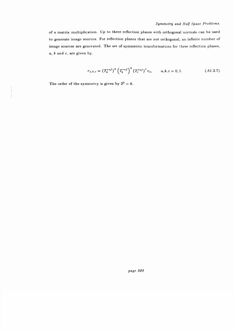
8/13/2019 Richard Jeans 1992 PhD Thesis
http://slidepdf.com/reader/full/richard-jeans-1992-phd-thesis 203/215
Symmetry and Half Space Problems.
of a matrix multiplication. Up to three reflection planes with orthogonal normals can be used
to generate image sources. For reflection planes that are not orthogonal, an infinite number of
imagesources are generated.
The
set of symmetrictransformations for
three reflection planes,
a, b and c, are given by,
ra, b,e =7ä ,f )a yreJ)b
TTref )Croe a, b, c = 0,1. A1.2.7)
The order of the symmetry is given by 23 = 8.
page 203

8/13/2019 Richard Jeans 1992 PhD Thesis
http://slidepdf.com/reader/full/richard-jeans-1992-phd-thesis 204/215
Symmetry and Half Space Problems.
U =o
Rigid Boundary
PressureRelease Boundary
Gk*_GkI+ Gk2
Geometric Symmetry
Figure (A1.2). Summary of image sources for the acoustic problem. The modi-
fied Green s function is denoted by G*.
page 204
un o

8/13/2019 Richard Jeans 1992 PhD Thesis
http://slidepdf.com/reader/full/richard-jeans-1992-phd-thesis 205/215
Analytical Series Solution for the Sphere.
APPENDIX 2.
Analytical Series Solution for the Sphere
A2.1 Rigid sphere
Throughout this study the spherical radiator is used to validate the acoustic numerical
methods since an analytical solution for the spherical problem is easily available. These results
are covered in great depth by Junger and Feit [1986], and they are summarized in this appendix.
The SHIE for the exterior problem is given by,
p(r) =
(p(ro)Or0) T_w2pwGk(r,ra) dSro, rEE, (A2.1.1)jo
where w is the radial displacement. If the coordinate system of the problem allows variable
separation of the Greens free space function, then an analytical solution is available. In spherical
polar coordinates the Greens free space function can be written in terms of spherical Besse]
functions and Legendre polynomials,
00 n
(2n + 1)cos m(0 - 00)k(r, O,01r, Bo Oo) =_ik Z
(n- m)1
47rn=o m=-n
(n + m) (A2.1.2)
Pn (cose)PP (coseo)jn(kro)hn(kr), r> ro
The coordinate system (r, 6, ¢) describes the exterior domain and (ro, Bo,0o) describes the
surface of the sphere. For coordinate systems where an analytical solution exists, the Green's
function in Eq. (A2.1.1) can be written as,
9(rß ro) = Gk (r, ro) + r(r, ro), (A2.1.3)
where F is a solution to the homogeneous Helmholtz' equation and the normal derivative of r
cancels the normal derivative of Gk on S. Consequently Eq. (A2.1.1) can be rewritten as,
P(r) = -,. )2p
iswg(r, ro)dSra,
,Js
r> r0. (A2.1.4)
page 205

8/13/2019 Richard Jeans 1992 PhD Thesis
http://slidepdf.com/reader/full/richard-jeans-1992-phd-thesis 206/215
Analytical Series Solution for the Sphere.
Taking the general case of ro =a the correct expression for g(r, r0), satisfying the homoge-
neous Neumann boundary condition and the radiation condition, is given by,
00 n
9(r, e, 0ja, 0,0o) =147rka2ZZ (n
- m)(2n + 1)cos m(¢ - 40)
n-o m. -n
(n + m).(. X2.1.5)
Pn (cosO)PP (cosOo)h'ý(ka)
r>a.n(
The exterior pressure field given in Eq. (A2.1.4) can now be written in terms of this modified
Green's function,
hn(kr)
ý)=2
oo n (n-rn)
( 2n + 1)(r B,47rk
n=0m=-n(n + m) hn (ka)
j2x
rJcos m(0 - 0)P(cosB)P(cosG0)sinBodBod0o, r a..
0(A2.1.6)
The radial displacement in Eq. (A2.1.6) can also be written as a summation of modal
displacements,
00 ný
W=1:1: WmmnuPP '(CO89o)COS
m'0. (A2.1.7)
nl=0 m'=-nl
When the modal expansion of w is substituted into Eq (A2.1.7), the orthogonality of the func-
tions simplifies the expression for the exterior pressure field,
2 °O n ftn kr
p(r, B, q) =-wkP EE WmnPn (cos9)cos mO h, (ka) ,r>a.,
(A2.1.8)
n-0 m--nn
where,
wmn =1(n - m)i (2n + 1) 2r Z Pn (cos90)cos m w(a, 90,ýo) sin90dO0dýo. (A2.1.9)
4ir n+m . ,0
j0()o
The pressure on the surface of the sphere can be expressed in terms of the modal impedance,
page 206

8/13/2019 Richard Jeans 1992 PhD Thesis
http://slidepdf.com/reader/full/richard-jeans-1992-phd-thesis 207/215
Analytical Series Solution for the Sphere.
00 n
P+(a, B,¢) = Z+,W,,,,,Pn (cosB)cos MO, (.12.1.10)Z
n-0 m--n
with,
zn = iPCh,(kQ)
(A2.1.11)
n()
The acoustic problem interior to thespherical shell can
beanalyzed
ina similar way.
The modified Green's function in Eq. (A2.1.5) must be constructed so that it satisfies the
homogeneous Neumann boundary condition and be finite as r-0. The corresponding surface
pressure on the interior surface is,
00 n
-(a, 8,0) = Zn Wmn P,, (cos9)cos MO, (A2.1.12)
n-0 m=-n
with,
?pCý;+(ka).
(A2.1.13)n
A comparison of Eq. (A2.1.11) and Eq. (A2.1.13) shows that whilst the exterior pressure
distribution is composed of a superposition of traveling waves, the interior pressure distribution is
a superposition of standing waves. The eigenvalues of the interior spherical problem correspond
to the solutions to,
zn (kD) = 0,
1
Ln=0(kN) .
(A2.1.14)
The interior eigenvalues for the spherical problem are tabulated in Table (A1.1) and the
frequency dependence of j and j;, is shown in figure (2.1).
page 207

8/13/2019 Richard Jeans 1992 PhD Thesis
http://slidepdf.com/reader/full/richard-jeans-1992-phd-thesis 208/215
Analytical Series Solution for the Sphere.
1.0
0.5
0.0
-0.50.000
0.4
0.2
0.0
-0.2
-0.4
-0.6`-0.0000 3.1416 6.2832 ka 9.4248
Figure (2.1). Plot of the first four spherical Bessel's functions and the deriva-
tives.
------------- ---------------1
3.142 6.284 ka 9.426
:. te ýý1
, ý' ý.
-------------- ------------- ---- - ----
Jý
page 208

8/13/2019 Richard Jeans 1992 PhD Thesis
http://slidepdf.com/reader/full/richard-jeans-1992-phd-thesis 209/215
Analytical Series Solution for the Sphere.
Dirichlet eigenvalues kD where j((kD), ) = 0.
1 n=0 n=1 n=2 n=3 n=4 n=5 n=6
1 3.141593 4.493409 5.763459 6.987932 8.182561 9.355812 10.512835
2 6.283185 7.725252 9.095011 10.417119 11.704907 12.966530 14.207392
3 9.424778 10.904122 12.322941 13.698023 15.039665 16.354710 17.647975
4 12.566371 14.066194 15.514603 16.923621 18.301256 19.653152 20.983463
Neumann eigenvalues kN where jn((kN)I) = 0.
1 n=0 n=1 n=2 n=3 n=4 n=5 n=6
1 4.493409 2.081576 3.342094 4.514100 5.646704 6.756456 7.851078
2 7.725252 5.940370 7.289932 8.583755 9.840446 11.070207 12.279334
3 10.904122 9.205840 10.613855 11.972730 13.295564 14.590552 15.863222
4 14.066194 12.404445 13.846112 15.244514 16.609346 17.947179 19.262710
Table (A2.1). The resonant frequencies for the interior spherical Dirichlet and
Neumann acoustic problems.
For any prescribed velocity distribution on the surface of the sphere the surface pressure
distribution may be calculated using Eq. (A2.1.10). For scattering from rigid spheres the surface
velocity must be equal to zero. Therefore the fluid particle velocity of the incident wave must
cancel that of the scattered wave. From the uniqueness of the external acoustic problem, the
scattered pressure field is obtained by solving the Helmholtz' reduced wave equation with the
virtual acceleration boundary condition,
iv, = -fi i=I
apion S. (A2.1.15)
An incident plane wave can be expanded in terms of spherical harmonics by using an addition
theorem,
00
p(r, O)
=P; E(2n + 1)i P(cosO)jn(kr). (A2.1.16)
n-0
Substituting Eq (A2.1.16) into Eq. (A2.1.15), Eq. (A2.1.8) gives an expression for the axisym-
metric scattered pressure field,
page 209

8/13/2019 Richard Jeans 1992 PhD Thesis
http://slidepdf.com/reader/full/richard-jeans-1992-phd-thesis 210/215
Analytical Series Solution for the Sphere.
00 hp5(r, O) = -Pi
E(2n+ 1)i Pn(cos9)
hn(ka)jn(kr) (. 2.1.17)
n. 0
The external pressure distribution is given by,
00 hn(kr).P(r, O)= p, + pi = PsE(2n + 1)inPn(cos8)
[n(kr)_
h, ka 7(kr) (A2.1.18)
n-0
li
n()
A2.2 Asymptotic solutions
The frequency dependence of the far field scattered pressure for an arbitrary geometry can
be approximated by asymptotic solutions. Consider Eq. (A2.1.17) in the far field,
00 1
psf (R, B) -ZPkR
Rj: (2n + 1)Pn(cos8)
hn(kr ,kR» n2 + 1. (A2.2.1)
n-0 n()
At low frequencies the first two terms of this series expansion are O((ka)2) and the n=2 term
is only O((ka)5). Taking the first two terms gives the far field pressure at low frequencies,
ikRep;
f (R, 8) =P3R
k2a33cosO
-1 k3a3 9 1, kR » 1. (A2.2.2)
The commensurate influence of monopole and dipole radiation in the far field, and the
consequent k2 dependence of the radiation amplitude is typical of Rayleigh Scatterers. A more
general consideration of such scatterers shows that at low frequencies the far field pressure
amplitude has the form,
ffk2V
k3L3«1, kR » 1.aR
where V is the volume and L is the characteristic dimension of the scatterer.
(. 2.2.3)
In the high frequency regime an approximation due to Kirchoff is appropriate. In this plane
wave approximation it is assumed that each surface element radiates as if it were in an plane
baffle,
page 210
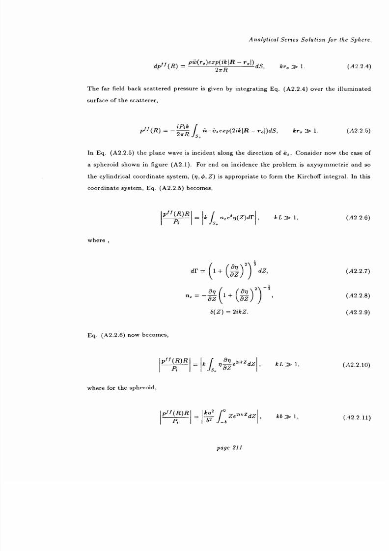
8/13/2019 Richard Jeans 1992 PhD Thesis
http://slidepdf.com/reader/full/richard-jeans-1992-phd-thesis 211/215
Analytical Series Solution for the Sphere.
dpP (R) -pw(ro)exp(ikIR - roI )dS,
kra » 1. (A2.2.4)
The far field back scattered pressure is given by integrating Eq. (A2.2.4) over the illuminated
surface of the scatterer,
_iP, kjf (R)2irR
n elexp(2ikIR- r0I)dS, kro » 1. (A2.2.5)
Is.
In Eq. (A2.2.5) the plane wave is incident along the direction of Z-,. Consider now the case of
a spheroid shown in figure (A2.1). For end on incidence the problem is axysymmetric and so
the cylindrical coordinate system, (q, 0, Z) is appropriate to form the Kirchoff integral. In this
coordinate system, Eq. (A2.2.5) becomes,
ptf (R)Rh-i k nze6T1(Z)dF,
kL» 1, (A2.2.6)Pi
is
where ,
2
dI' =1+ azdZ, (A2.2.7)
2
nz öZ+
az(A2.2.8)
b(Z) = 2ikZ. (A2.2.9)
Eq. (A2.2.6) now becomes,
pof (R)Rk
ýZeaikZdZ kL » 1, (A2.2.10)
J,
where for the spheroid,
p'f (R) R_ ka2 0ZezikzdZ
,kb » 1,
pi b2
fb(.2.2.11)
page 211

8/13/2019 Richard Jeans 1992 PhD Thesis
http://slidepdf.com/reader/full/richard-jeans-1992-phd-thesis 212/215
Analytical Series Solution for the Sphere.
Inctuerli rruve
Figure A0. L). Geometry for the spheroidal Kirchof problem.
The integral in Eq. A2.2.11) can be done in parts, and neglecting the terms of O kb)-1
or higher the high frequency far field back scattering amplitude is given by,
pof R)R a2 kb » 1.Pi
I= I2l,A2.2.12)
This is the result used in Chapter 4, and for the special case of the sphere, with b=a, it
reduces to the spherical result used in Chapter 3. If higher frequency terms are included an
interference pattern is introduced into the farfield result. This interference corresponds to a
path difference of 2b; ie the path difference between a specular wave at Z=-b and one at
Z=0. The numerical results contained in this thesis show such an interfence pattern, however
the period of the fluctuations are much less than those predicted by the Kirchoff approximation.
The accepted explanation for the interference pattern eg Varadan et al [1982]) is that they are
a result of the interference between the specular reflection at Z= -b and a Franz or creeping
wave originating at the circular cross section at b=0. The predicted period of the interference
is given by,
A kb)27
,D -+2 A2.2.13)
where D is one half the perimeter of the spheroid in the X=0 plane. For the various aspect
ratios used in this study this period is,
page 212

8/13/2019 Richard Jeans 1992 PhD Thesis
http://slidepdf.com/reader/full/richard-jeans-1992-phd-thesis 213/215
Analytical Series Solution for the Sphere.
alb = 0.5, z(kb) -- 1.42,
alb = 1,0(kb) = 1.22,
alb = 2,0(kb) = 2.84,
A2.3 Elastic sphere
J(ka) = 0.71,
J(ka) = 1.22, (A2.2.14)
0(ka) = 1.42.
For axisymmetric boundary conditions, there is a readily accessible analytical solution for
the dynamic elastic response of the spherical elastic shell. This solution is described in greater
depth in many standard texts, and is summarized in this appendix. Membrane and flexural
effects are included in the analytical model which can be derived from Hamilton s variational
principle. Many of the thin shell approximations used for the finite element derivation are
used for the analytical result; ie the deformation can be described in terms of the mid-shell
displacements and the mid-shell normal is remains straight after deformation.
Axisymmetric, nontortional motions are considered and the shell displacements can be
described in terms of the tangential and radial components; ur and ue. A free dynamic analysis
of the shell results in an expression for the dimensionless natural frequencies, (5l )2 and (52,, )2,
which are roots of a quadratic in Q2,
524- [1+3v+A-/32(1-v-An-vAn)]
52+(AT-2)(1-v2)+
(A2.3.1)
ß2 [An-4,n+An(5-v2)-2(1-v2)] =0,
where,
=ca, Q =
h2
1222An = n(n + 1). (A2.3.2)
P
The radial or normal and the tangential displacements can be expanded in terms of Legendre
polynomials,
00
ur =1: WWPn(µ),
n=O
°°P2)1/2
dPn(p) (A2.3.3)
n=0dp
p=COSO.
page 213

8/13/2019 Richard Jeans 1992 PhD Thesis
http://slidepdf.com/reader/full/richard-jeans-1992-phd-thesis 214/215
Analytical Series Solution for the Sphere.
For forced vibration of the spherical shell, the modal radial amplitude is related to the
modal force amplitude by,
ýn =_
fn
__
IP, cp h [c2-
(c(1))2] [92-
(9(2»2,(A2.3.4)
2wwn 9 a[92- (1- QZ)(v + An - 1)]
where the modal excitation force is given by,
(2n + l) 1fn =2f f(µ)P (µ)dp. (A2.3.5)
i
Finally the modal radial and tangential amplitudes are related by,
V_
[32(v+A- 1)+(i+ v)] (A2.3.6)
For a spherical shell vibrating in an acoustic fluid, the excitation force in Eq. (A2.3.5)
consists of the apllied force, f', modified by the fluid-structure interaction force, f'. The modal
normal velocity of the submerged spherical shell is given by,
Z,n=fn -. fn, (A2.3.7)
where,
fn= Pn - Pn = ýz - zn ] Wn. (A2.3.8)
Therefore by combining Eq. (A2.3.7) and Eq. (A2.3.8) the surface pressure and velocity
fields for the excited spherical shell are given by,
°O fa
un (a, e)=Zn_ PP (cose),
[Zn + Zn - Zni=0
0o a
P(a, 0) =Z
Zn+ fn
_P1 (COSB).
i-0 `Zn+ Zn - zn
For the point excited spherical shell the modal excitation force is defined by,
(A2.3.9)
page 214
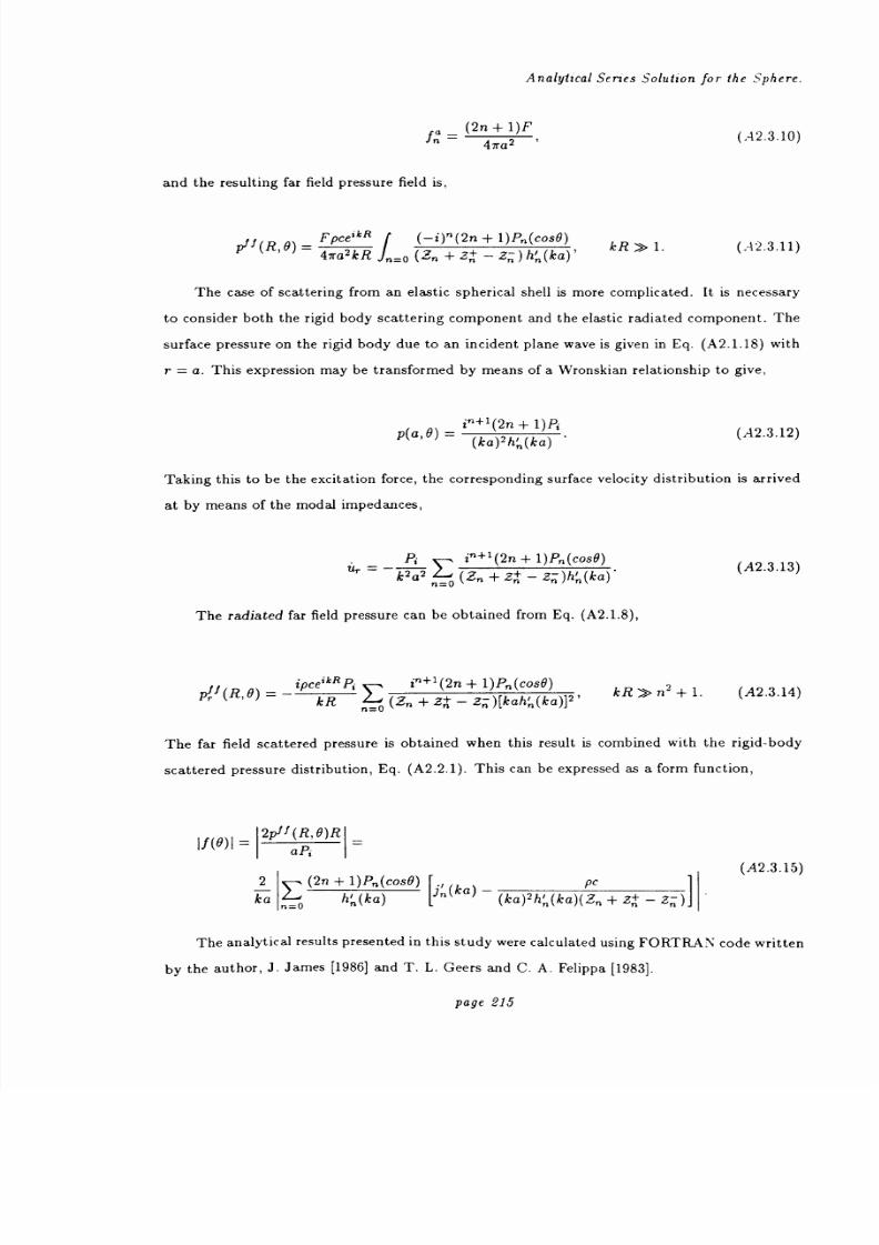
8/13/2019 Richard Jeans 1992 PhD Thesis
http://slidepdf.com/reader/full/richard-jeans-1992-phd-thesis 215/215
Analytical Series Solution for the Sphere.
a_-(2n + 1)F
(.-2.3.10)"47ra2
and the resulting far field pressure field is,
pff(R, B)
-
Fpce'kR (-i)n(2n+ 1)Pn(cos8)kR» 1. (A2.3.11)
=o(2n + Z+ - -n)h' (ka)'7razkR J n
The case of scattering from an elastic spherical shell is more complicated. It is necessary
to consider both the rigid body scattering component and the elastic radiated component. The
surface pressure on the rigid body due to an incident plane wave is given in Eq. (A2.1.18) with


![[Architecture eBook] Richard Meier Architect, Vol 3 (1992-1998), Rizzoli, 1999_dg2005](https://img.pdfslide.us/doc/110x75/55cf8f40550346703b9a74b4/architecture-ebook-richard-meier-architect-vol-3-1992-1998-rizzoli-1999dg2005.jpg)