Rich feature hierarchies for accurate object detection and semantic segmentation

Ross Girshick, Jeff Donahue, Trevor Darrell, Jitendra Malik UC Berkeley

!

Tech Report @ http://arxiv.org/abs/1311.2524

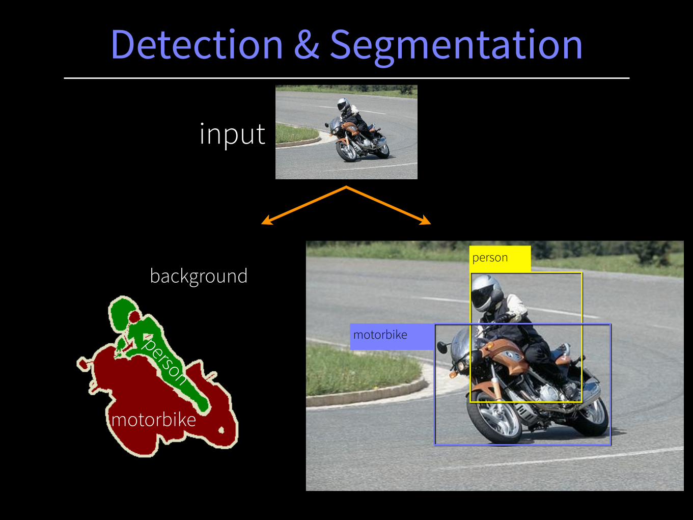
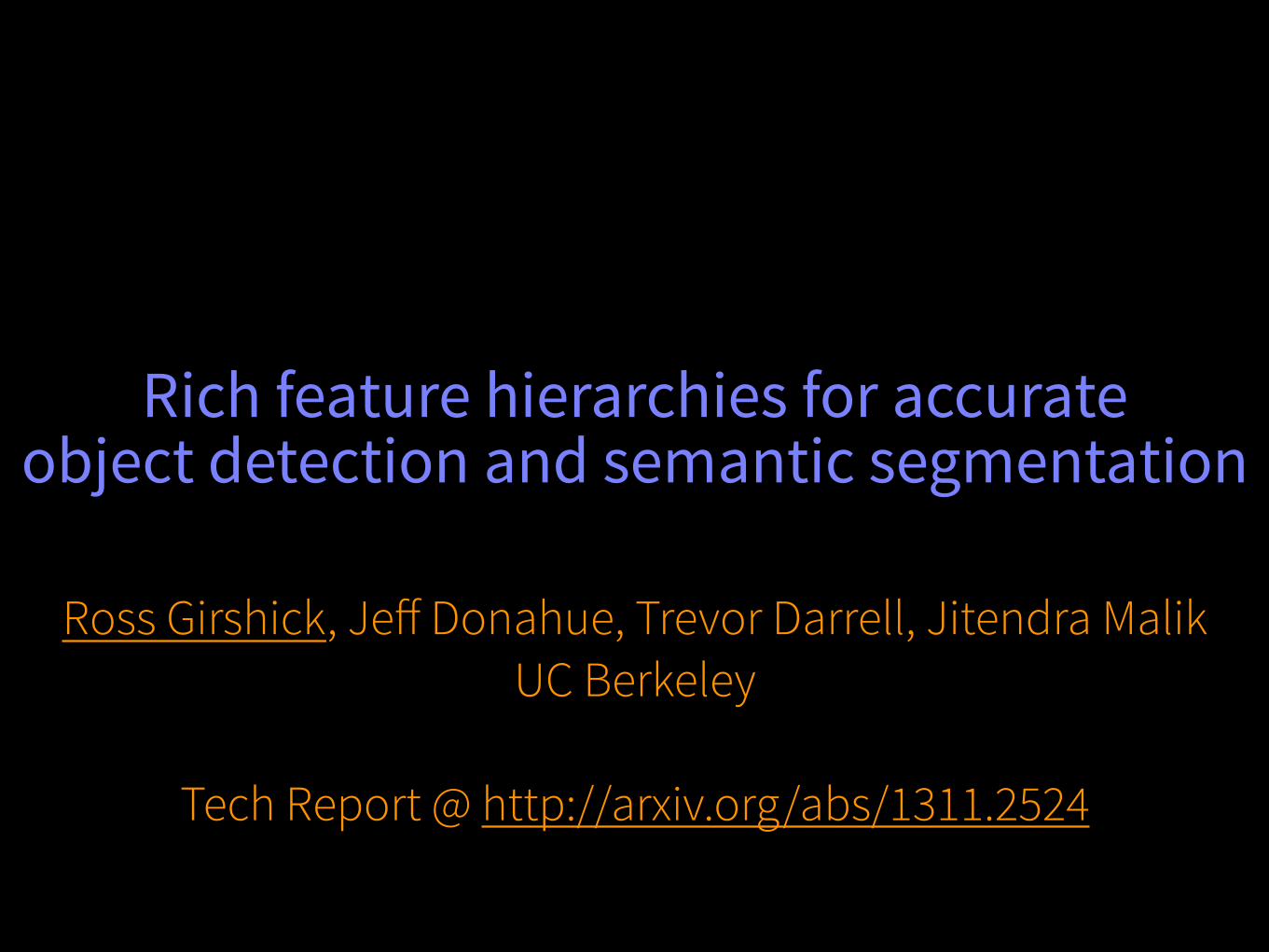
Detection & Segmentation

person

motorbike

motorbike

person

background

input

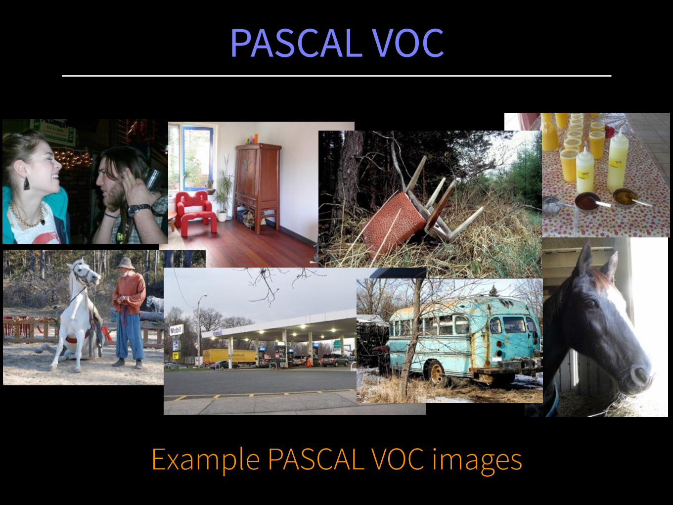
PASCAL VOC

Example PASCAL VOC images

1. Part-based sliding window methods (HOG)

Dominant detection methods

DPM Poselets

Russell et al. 2006 Gu et al. 2009 van de Sande et al. 2011 > “selective search”

2. Region-proposal classifiers (SIFT++ BoW)

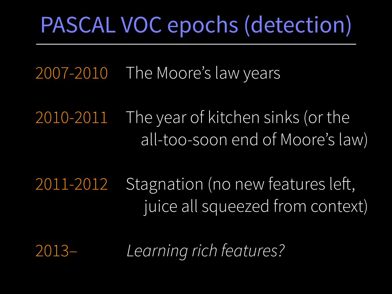
2007-2010 The Moore’s law years !

2010-2011 The year of kitchen sinks (or the all-too-soon end of Moore’s law) !

2011-2012 Stagnation (no new features left, juice all squeezed from context) !

2013– Learning rich features?

PASCAL VOC epochs (detection)

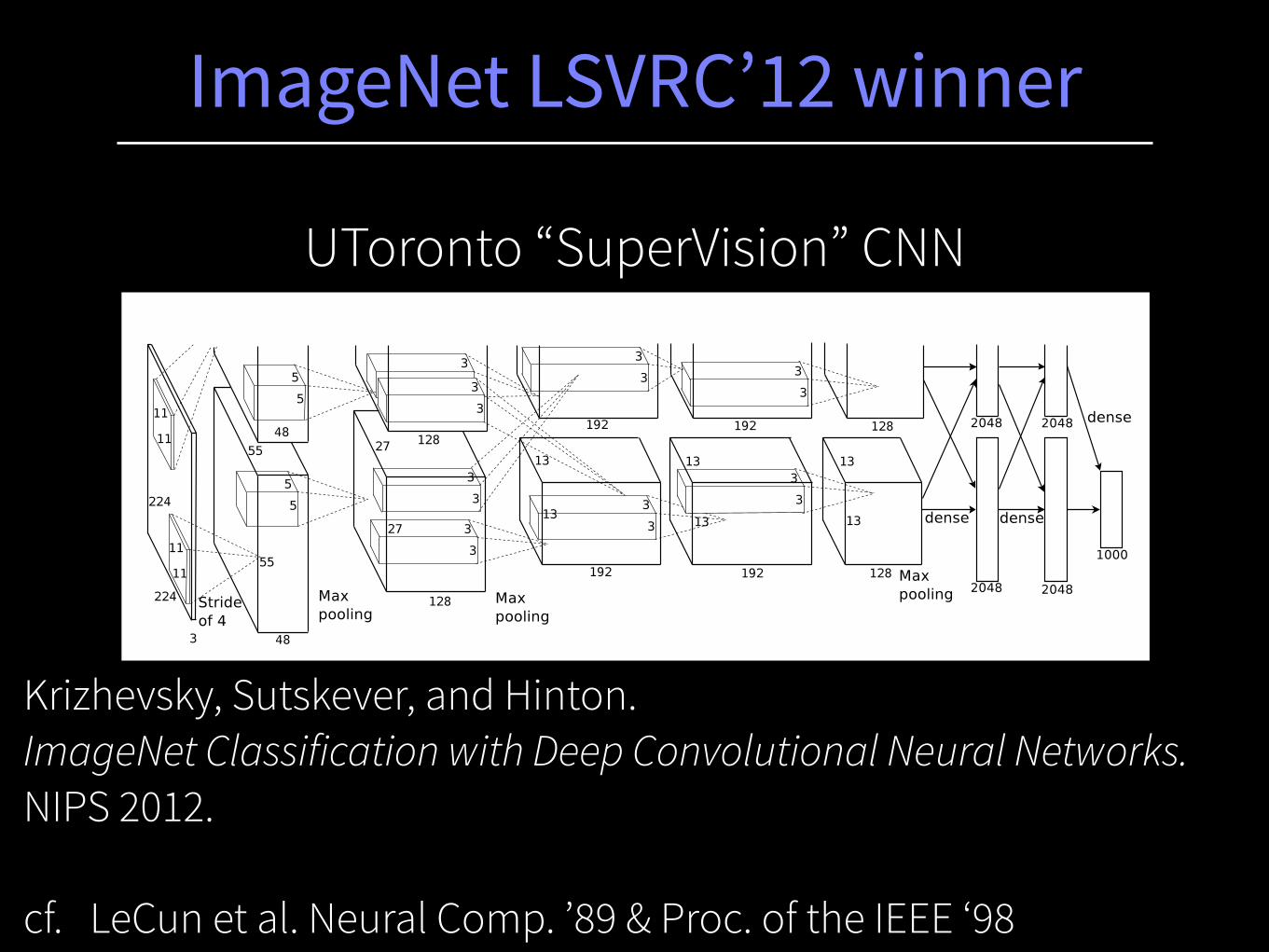
UToronto “SuperVision” CNN

ImageNet LSVRC’12 winner

Figure 2: An illustration of the architecture of our CNN, explicitly showing the delineation of responsibilitiesbetween the two GPUs. One GPU runs the layer-parts at the top of the figure while the other runs the layer-partsat the bottom. The GPUs communicate only at certain layers. The network’s input is 150,528-dimensional, andthe number of neurons in the network’s remaining layers is given by 253,440–186,624–64,896–64,896–43,264–4096–4096–1000.

neurons in a kernel map). The second convolutional layer takes as input the (response-normalizedand pooled) output of the first convolutional layer and filters it with 256 kernels of size 5⇥ 5⇥ 48.The third, fourth, and fifth convolutional layers are connected to one another without any interveningpooling or normalization layers. The third convolutional layer has 384 kernels of size 3 ⇥ 3 ⇥256 connected to the (normalized, pooled) outputs of the second convolutional layer. The fourthconvolutional layer has 384 kernels of size 3 ⇥ 3 ⇥ 192 , and the fifth convolutional layer has 256kernels of size 3⇥ 3⇥ 192. The fully-connected layers have 4096 neurons each.

4 Reducing Overfitting

Our neural network architecture has 60 million parameters. Although the 1000 classes of ILSVRCmake each training example impose 10 bits of constraint on the mapping from image to label, thisturns out to be insufficient to learn so many parameters without considerable overfitting. Below, wedescribe the two primary ways in which we combat overfitting.

4.1 Data Augmentation

The easiest and most common method to reduce overfitting on image data is to artificially enlargethe dataset using label-preserving transformations (e.g., [25, 4, 5]). We employ two distinct formsof data augmentation, both of which allow transformed images to be produced from the originalimages with very little computation, so the transformed images do not need to be stored on disk.In our implementation, the transformed images are generated in Python code on the CPU while theGPU is training on the previous batch of images. So these data augmentation schemes are, in effect,computationally free.

The first form of data augmentation consists of generating image translations and horizontal reflec-tions. We do this by extracting random 224⇥ 224 patches (and their horizontal reflections) from the256⇥256 images and training our network on these extracted patches4. This increases the size of ourtraining set by a factor of 2048, though the resulting training examples are, of course, highly inter-dependent. Without this scheme, our network suffers from substantial overfitting, which would haveforced us to use much smaller networks. At test time, the network makes a prediction by extractingfive 224 ⇥ 224 patches (the four corner patches and the center patch) as well as their horizontalreflections (hence ten patches in all), and averaging the predictions made by the network’s softmaxlayer on the ten patches.

The second form of data augmentation consists of altering the intensities of the RGB channels intraining images. Specifically, we perform PCA on the set of RGB pixel values throughout theImageNet training set. To each training image, we add multiples of the found principal components,

4This is the reason why the input images in Figure 2 are 224⇥ 224⇥ 3-dimensional.

5

Krizhevsky, Sutskever, and Hinton. ImageNet Classification with Deep Convolutional Neural Networks. NIPS 2012. !cf. LeCun et al. Neural Comp. ’89 & Proc. of the IEEE ‘98

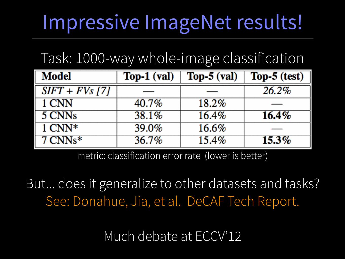
Impressive ImageNet results!

But... does it generalize to other datasets and tasks? See: Donahue, Jia, et al. DeCAF Tech Report.

!

Much debate at ECCV’12

Task: 1000-way whole-image classification

metric: classification error rate (lower is better)

Understand if the SuperVision CNN can be made to work as an object detector.

Objective

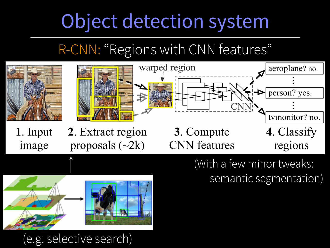
Object detection system

1. Input image

2. Extract region proposals (~2k)

3. Compute CNN features

aeroplane? no.

...person? yes.

tvmonitor? no.

4. Classify regions

warped region...

CNN

(e.g. selective search)

(With a few minor tweaks: semantic segmentation)

R-CNN: “Regions with CNN features”

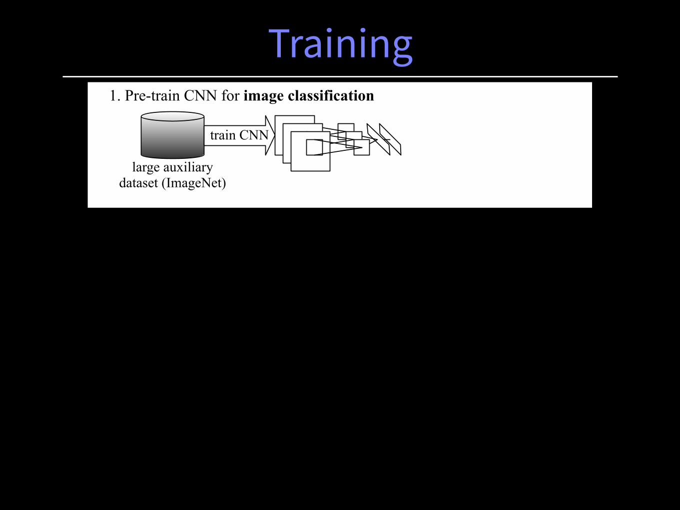
Training

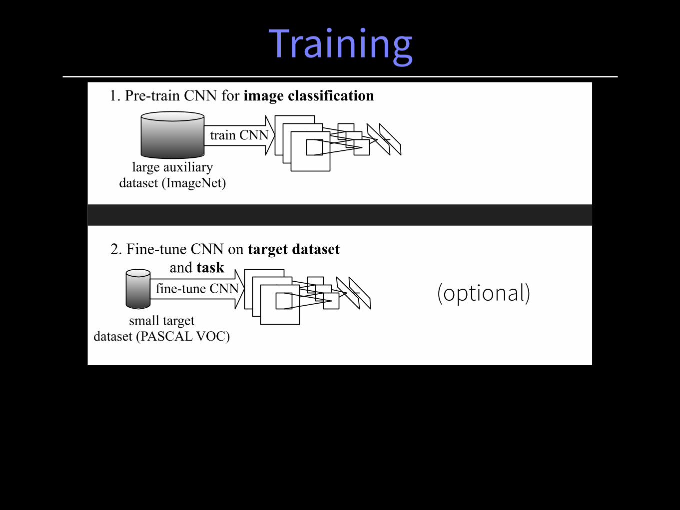
large auxiliary dataset (ImageNet)

train CNN

1. Pre-train CNN for image classification

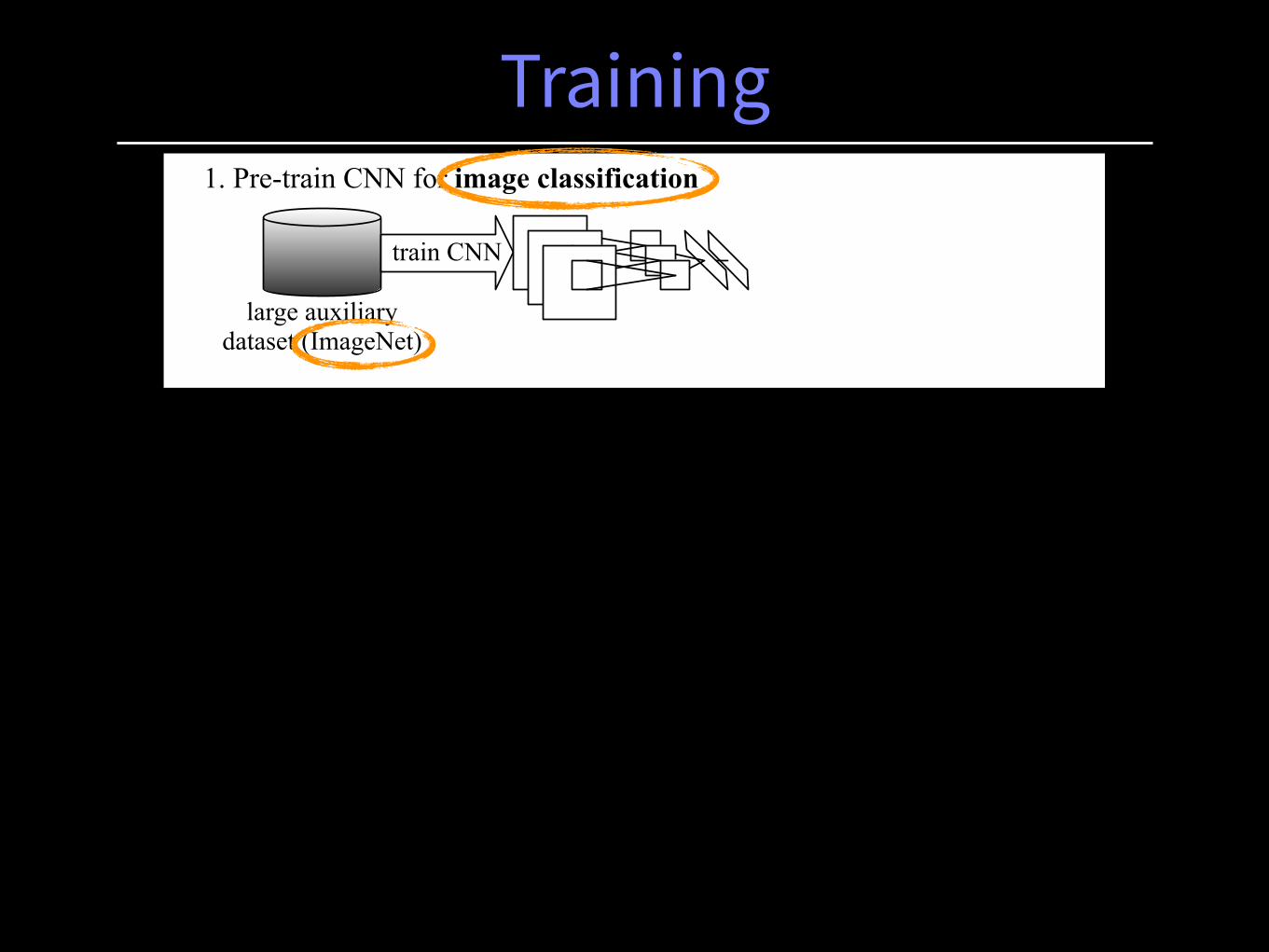
Training

large auxiliary dataset (ImageNet)

train CNN

1. Pre-train CNN for image classification

Training

large auxiliary dataset (ImageNet)

train CNN

1. Pre-train CNN for image classification

small targetdataset (PASCAL VOC)

fine-tune CNN

2. Fine-tune CNN on target dataset and task

(optional)

Training

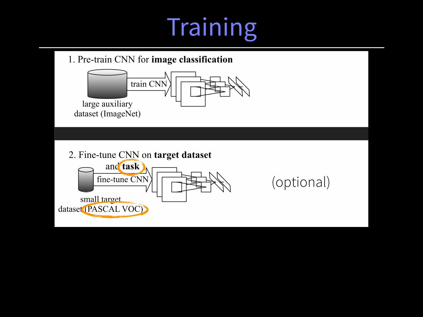
large auxiliary dataset (ImageNet)

train CNN

1. Pre-train CNN for image classification

small targetdataset (PASCAL VOC)

fine-tune CNN

2. Fine-tune CNN on target dataset and task

(optional)

Training

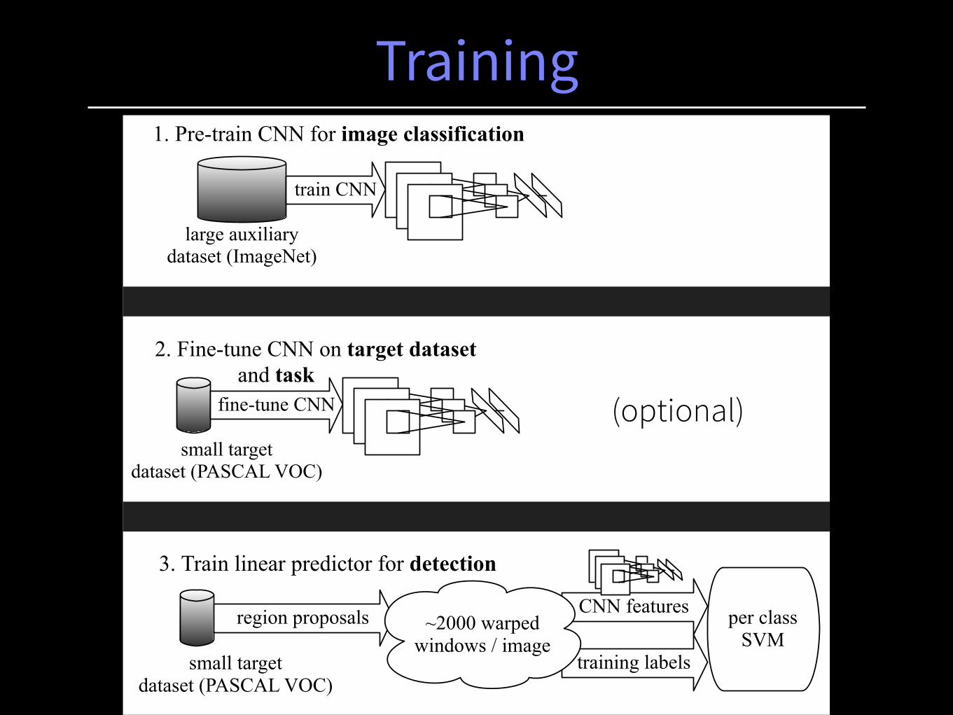
large auxiliary dataset (ImageNet)

train CNN

1. Pre-train CNN for image classification

training labels

3. Train linear predictor for detection

small targetdataset (PASCAL VOC)

region proposals CNN features~2000 warped

windows / imageper class

SVM

small targetdataset (PASCAL VOC)

fine-tune CNN

2. Fine-tune CNN on target dataset and task

(optional)

Training labels

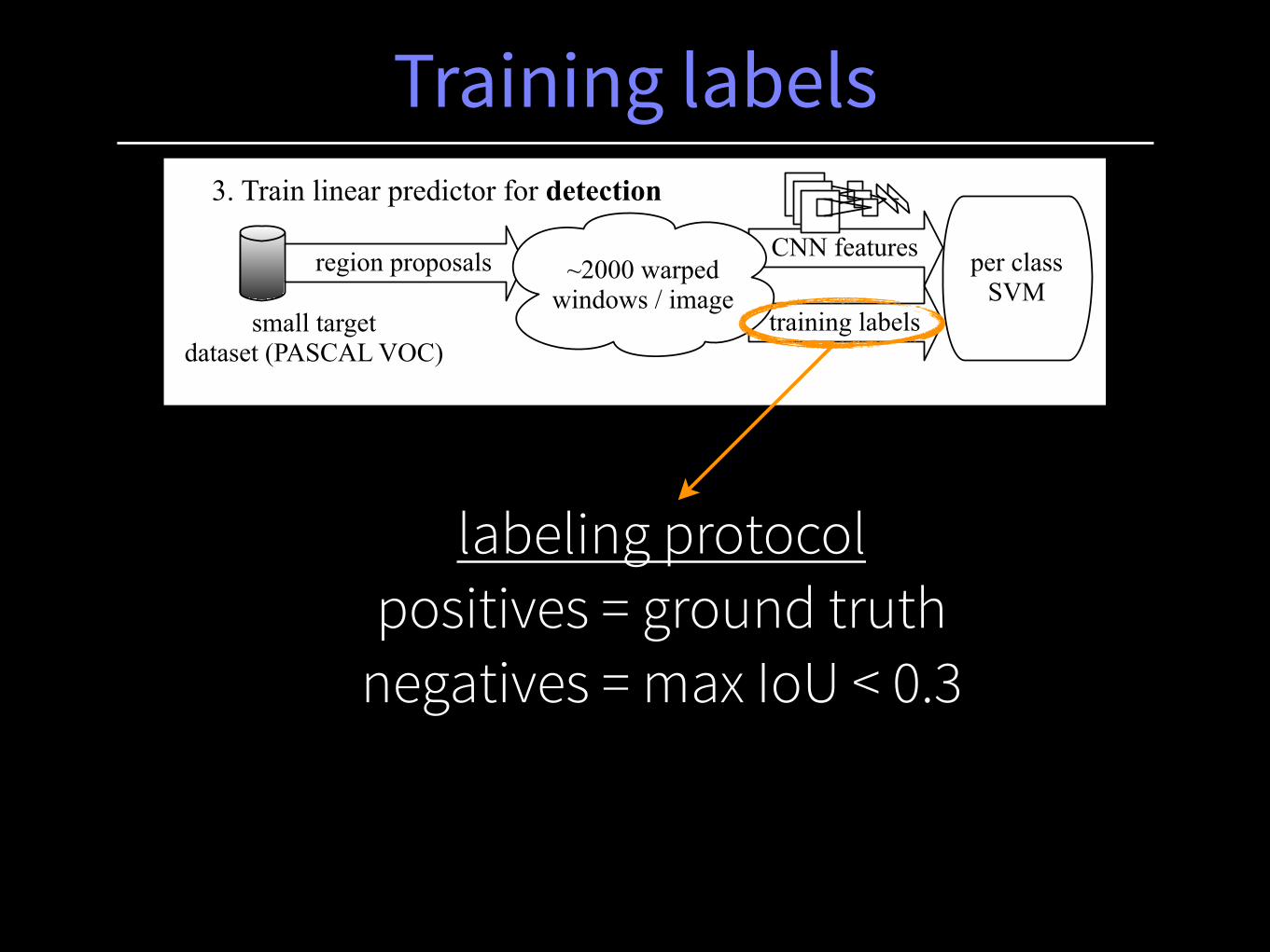
labeling protocol positives = ground truth

negatives = max IoU < 0.3

training labels

3. Train linear predictor for detection

small targetdataset (PASCAL VOC)

region proposals CNN features~2000 warped

windows / imageper class

SVM

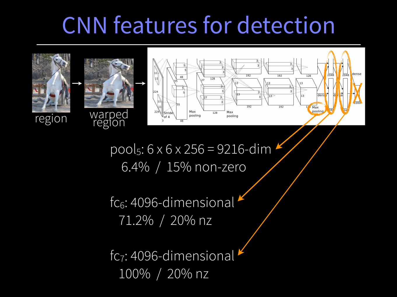
CNN features for detection

Figure 2: An illustration of the architecture of our CNN, explicitly showing the delineation of responsibilitiesbetween the two GPUs. One GPU runs the layer-parts at the top of the figure while the other runs the layer-partsat the bottom. The GPUs communicate only at certain layers. The network’s input is 150,528-dimensional, andthe number of neurons in the network’s remaining layers is given by 253,440–186,624–64,896–64,896–43,264–4096–4096–1000.

neurons in a kernel map). The second convolutional layer takes as input the (response-normalizedand pooled) output of the first convolutional layer and filters it with 256 kernels of size 5⇥ 5⇥ 48.The third, fourth, and fifth convolutional layers are connected to one another without any interveningpooling or normalization layers. The third convolutional layer has 384 kernels of size 3 ⇥ 3 ⇥256 connected to the (normalized, pooled) outputs of the second convolutional layer. The fourthconvolutional layer has 384 kernels of size 3 ⇥ 3 ⇥ 192 , and the fifth convolutional layer has 256kernels of size 3⇥ 3⇥ 192. The fully-connected layers have 4096 neurons each.

4 Reducing Overfitting

Our neural network architecture has 60 million parameters. Although the 1000 classes of ILSVRCmake each training example impose 10 bits of constraint on the mapping from image to label, thisturns out to be insufficient to learn so many parameters without considerable overfitting. Below, wedescribe the two primary ways in which we combat overfitting.

4.1 Data Augmentation

The easiest and most common method to reduce overfitting on image data is to artificially enlargethe dataset using label-preserving transformations (e.g., [25, 4, 5]). We employ two distinct formsof data augmentation, both of which allow transformed images to be produced from the originalimages with very little computation, so the transformed images do not need to be stored on disk.In our implementation, the transformed images are generated in Python code on the CPU while theGPU is training on the previous batch of images. So these data augmentation schemes are, in effect,computationally free.

The first form of data augmentation consists of generating image translations and horizontal reflec-tions. We do this by extracting random 224⇥ 224 patches (and their horizontal reflections) from the256⇥256 images and training our network on these extracted patches4. This increases the size of ourtraining set by a factor of 2048, though the resulting training examples are, of course, highly inter-dependent. Without this scheme, our network suffers from substantial overfitting, which would haveforced us to use much smaller networks. At test time, the network makes a prediction by extractingfive 224 ⇥ 224 patches (the four corner patches and the center patch) as well as their horizontalreflections (hence ten patches in all), and averaging the predictions made by the network’s softmaxlayer on the ten patches.

The second form of data augmentation consists of altering the intensities of the RGB channels intraining images. Specifically, we perform PCA on the set of RGB pixel values throughout theImageNet training set. To each training image, we add multiples of the found principal components,

4This is the reason why the input images in Figure 2 are 224⇥ 224⇥ 3-dimensional.

5

pool5: 6 x 6 x 256 = 9216-dim 6.4% / 15% non-zero !

fc6: 4096-dimensional 71.2% / 20% nz !

fc7: 4096-dimensional 100% / 20% nz

region warped region

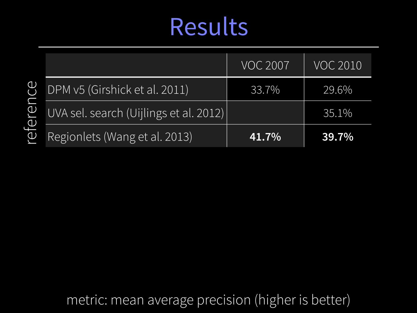
Results

metric: mean average precision (higher is better)

VOC 2007 VOC 2010

DPM v5 (Girshick et al. 2011) 33.7% 29.6%

UVA sel. search (Uijlings et al. 2012) 35.1%

Regionlets (Wang et al. 2013) 41.7% 39.7%

R-CNN pool5 40.1%

R-CNN fc6 43.4%

R-CNN fc7 42.6%

R-CNN FT pool5 42.1%

R-CNN FT fc6 47.2%

R-CNN FT fc7 48% 43.5%

refe

renc

e

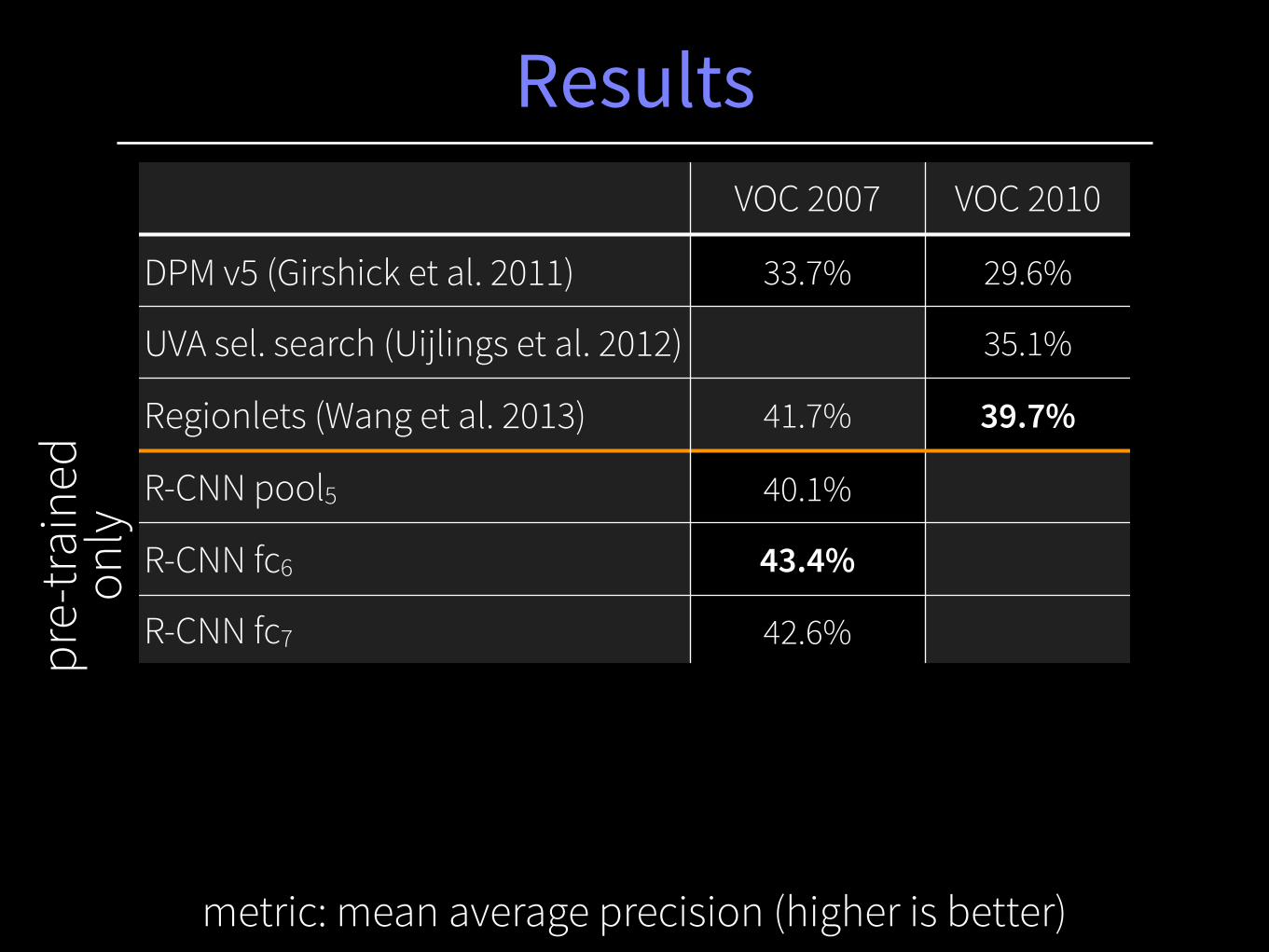
Resultspr

e-tra

ined

on

ly

metric: mean average precision (higher is better)

VOC 2007 VOC 2010

DPM v5 (Girshick et al. 2011) 33.7% 29.6%

UVA sel. search (Uijlings et al. 2012) 35.1%

Regionlets (Wang et al. 2013) 41.7% 39.7%

R-CNN pool5 40.1%

R-CNN fc6 43.4%

R-CNN fc7 42.6%

R-CNN FT pool5 42.1%

R-CNN FT fc6 47.2%

R-CNN FT fc7 48% 43.5%

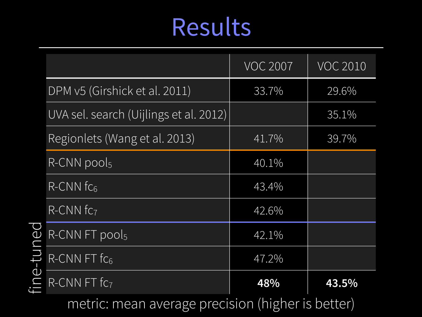
Resultsfin

e-tu

ned

metric: mean average precision (higher is better)

VOC 2007 VOC 2010

DPM v5 (Girshick et al. 2011) 33.7% 29.6%

UVA sel. search (Uijlings et al. 2012) 35.1%

Regionlets (Wang et al. 2013) 41.7% 39.7%

R-CNN pool5 40.1%

R-CNN fc6 43.4%

R-CNN fc7 42.6%

R-CNN FT pool5 42.1%

R-CNN FT fc6 47.2%

R-CNN FT fc7 48% 43.5%

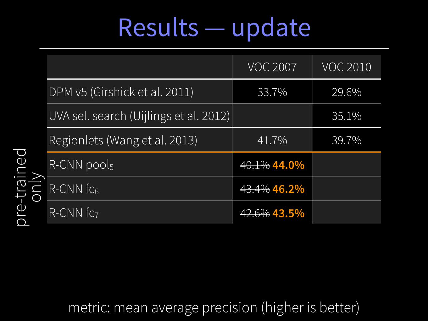
Results — updateVOC 2007 VOC 2010

DPM v5 (Girshick et al. 2011) 33.7% 29.6%

UVA sel. search (Uijlings et al. 2012) 35.1%

Regionlets (Wang et al. 2013) 41.7% 39.7%

R-CNN pool5 40.1% 44.0%

R-CNN fc6 43.4% 46.2%

R-CNN fc7 42.6% 43.5%

R-CNN FT pool5 42.1%

R-CNN FT fc6 47.2%

R-CNN FT fc7 48% 43.5%

metric: mean average precision (higher is better)

pre-

train

ed

only

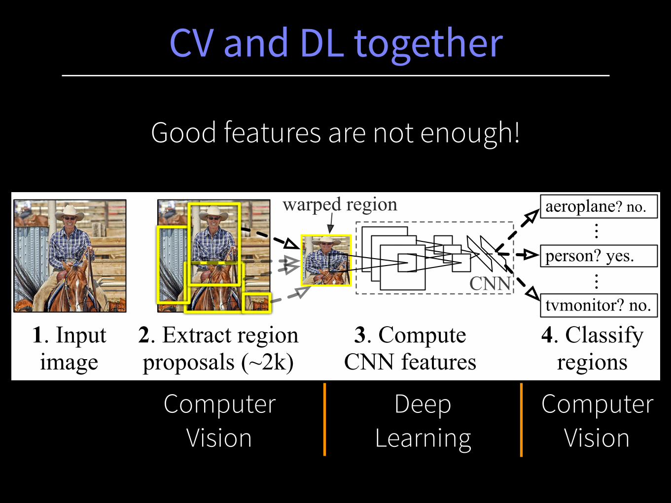
CV and DL together

1. Input image

2. Extract region proposals (~2k)

3. Compute CNN features

aeroplane? no.

...person? yes.

tvmonitor? no.

4. Classify regions

warped region...

CNN

Computer Vision

Deep Learning

Computer Vision

Good features are not enough!

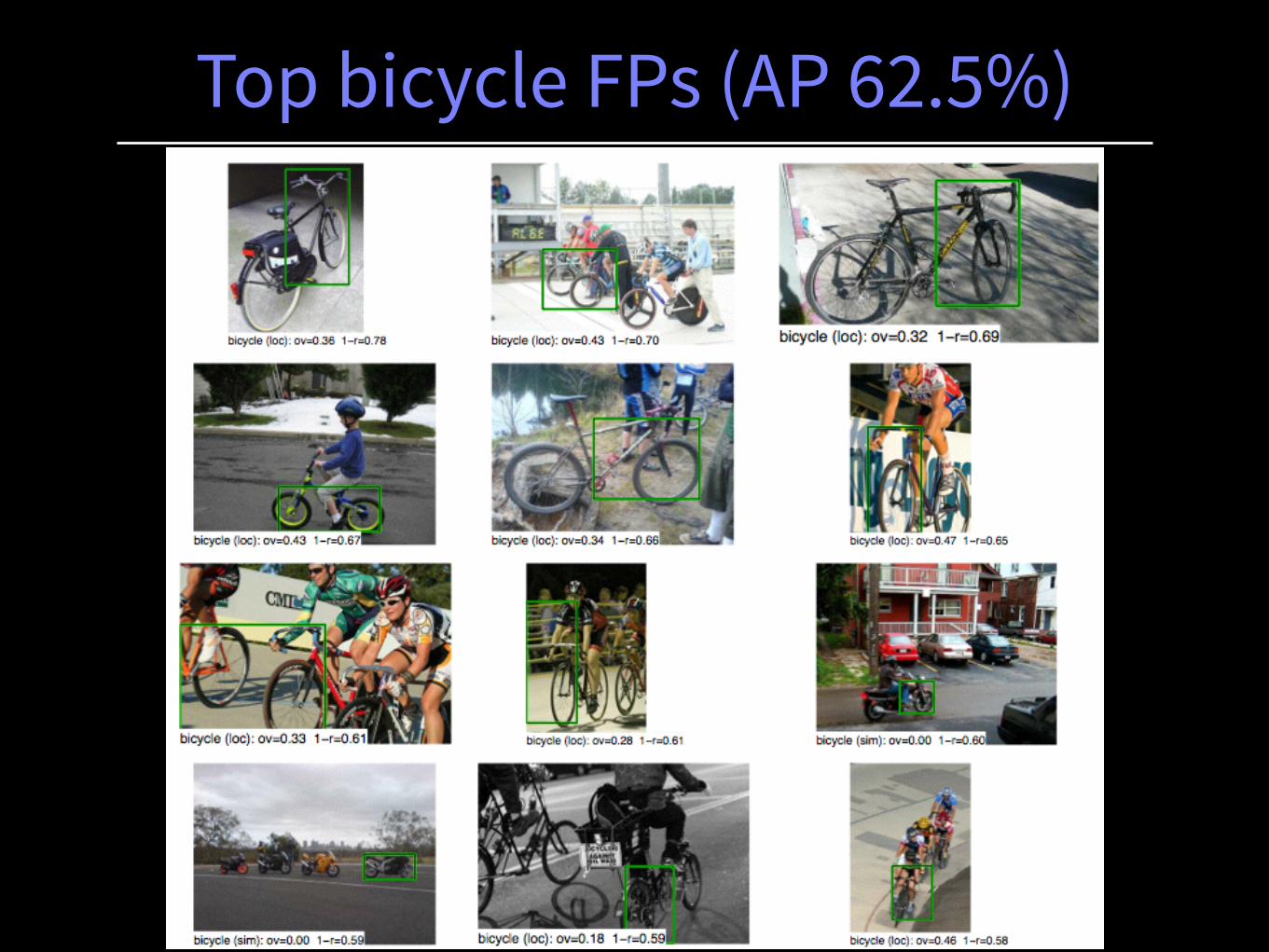
Top bicycle FPs (AP 62.5%)

Top bird FPs (AP 41.4%)

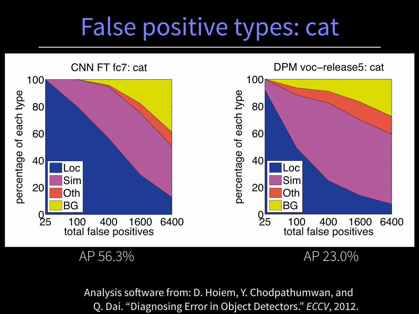
False positive types: cat

Analysis software from: D. Hoiem, Y. Chodpathumwan, and Q. Dai. “Diagnosing Error in Object Detectors.” ECCV, 2012.

total false positives

perc

enta

ge o

f eac

h ty

pe

CNN FT fc7: cat

25 100 400 1600 64000

20

40

60

80

100

LocSimOthBG

total false positivespe

rcen

tage

of e

ach

type

DPM voc−release5: cat

25 100 400 1600 64000

20

40

60

80

100

LocSimOthBG

AP 56.3% AP 23.0%

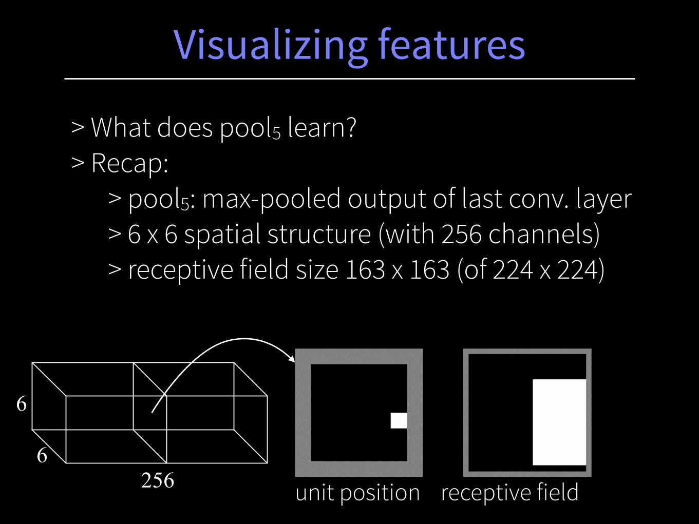
> What does pool5 learn? > Recap:

> pool5: max-pooled output of last conv. layer > 6 x 6 spatial structure (with 256 channels) > receptive field size 163 x 163 (of 224 x 224)

Visualizing features

unit position receptive field2566

6

> Select a unit in pool5 > Run it as a detector > Show top-scoring regions > Non-parametric, lets unit “speak for itself” !

!

!

(Used ~10 million held-out regions.)

Visualization method

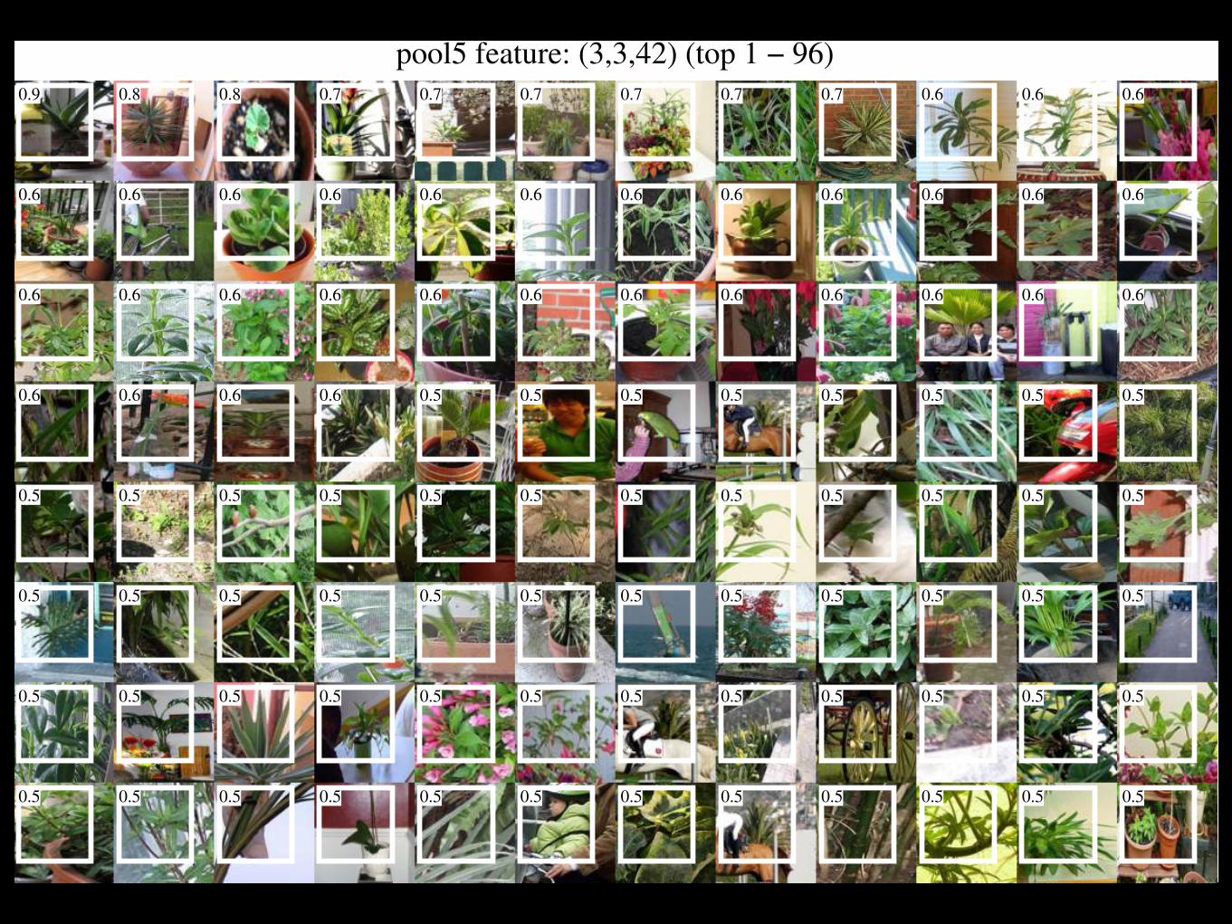
pool5 feature: (3,3,42) (top 1 − 96)0.9 0.8 0.8 0.7 0.7 0.7 0.7 0.7 0.7 0.6 0.6 0.6

0.6 0.6 0.6 0.6 0.6 0.6 0.6 0.6 0.6 0.6 0.6 0.6

0.6 0.6 0.6 0.6 0.6 0.6 0.6 0.6 0.6 0.6 0.6 0.6

0.6 0.6 0.6 0.6 0.5 0.5 0.5 0.5 0.5 0.5 0.5 0.5

0.5 0.5 0.5 0.5 0.5 0.5 0.5 0.5 0.5 0.5 0.5 0.5

0.5 0.5 0.5 0.5 0.5 0.5 0.5 0.5 0.5 0.5 0.5 0.5

0.5 0.5 0.5 0.5 0.5 0.5 0.5 0.5 0.5 0.5 0.5 0.5

0.5 0.5 0.5 0.5 0.5 0.5 0.5 0.5 0.5 0.5 0.5 0.5

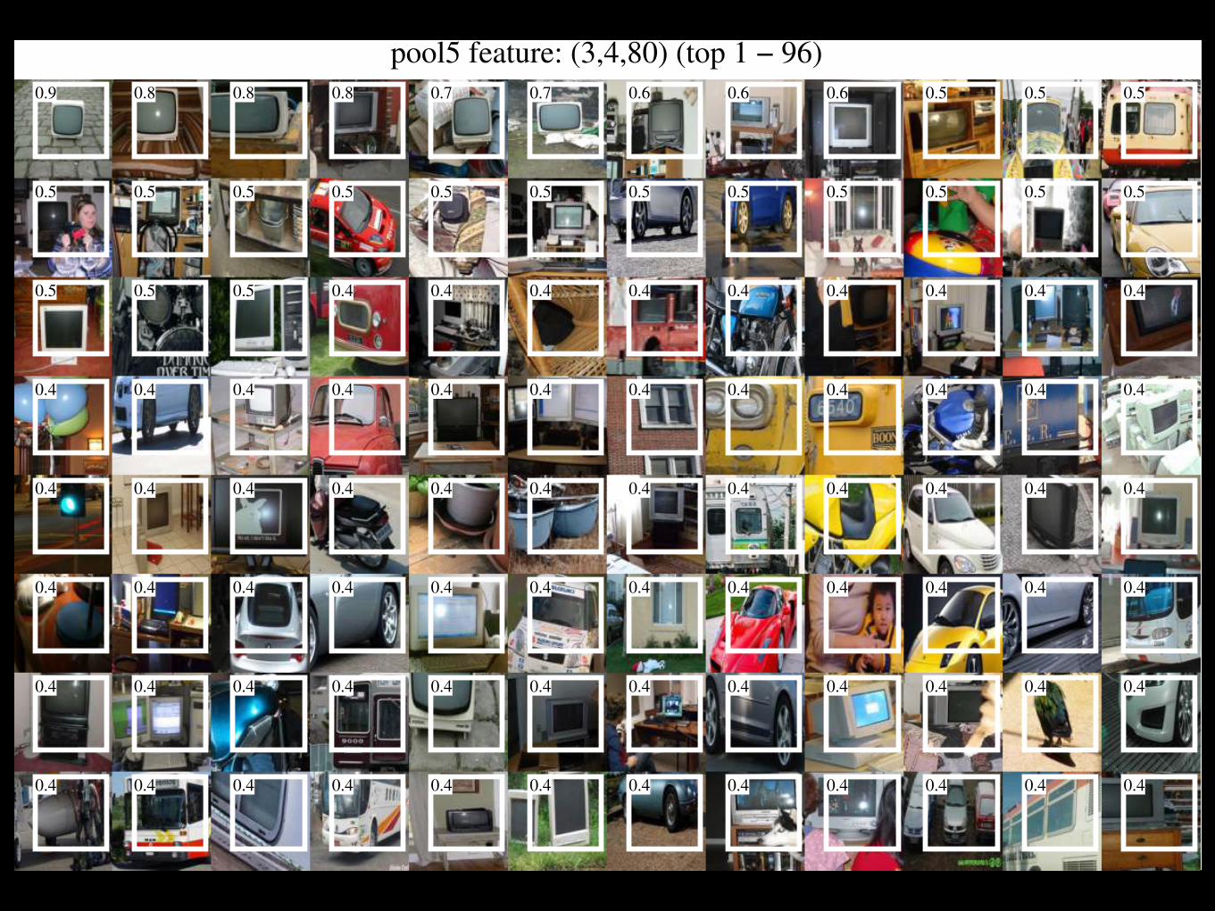
pool5 feature: (3,4,80) (top 1 − 96)0.9 0.8 0.8 0.8 0.7 0.7 0.6 0.6 0.6 0.5 0.5 0.5

0.5 0.5 0.5 0.5 0.5 0.5 0.5 0.5 0.5 0.5 0.5 0.5

0.5 0.5 0.5 0.4 0.4 0.4 0.4 0.4 0.4 0.4 0.4 0.4

0.4 0.4 0.4 0.4 0.4 0.4 0.4 0.4 0.4 0.4 0.4 0.4

0.4 0.4 0.4 0.4 0.4 0.4 0.4 0.4 0.4 0.4 0.4 0.4

0.4 0.4 0.4 0.4 0.4 0.4 0.4 0.4 0.4 0.4 0.4 0.4

0.4 0.4 0.4 0.4 0.4 0.4 0.4 0.4 0.4 0.4 0.4 0.4

0.4 0.4 0.4 0.4 0.4 0.4 0.4 0.4 0.4 0.4 0.4 0.4

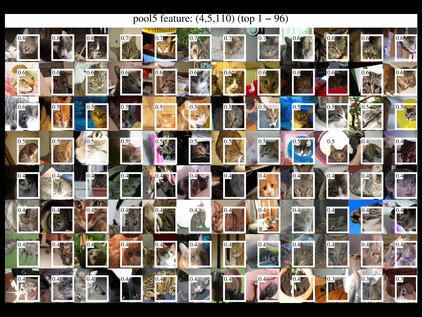
pool5 feature: (4,5,110) (top 1 − 96)

0.8 0.8 0.8 0.7 0.7 0.7 0.7 0.7 0.6 0.6 0.6 0.6

0.6 0.6 0.6 0.6 0.6 0.6 0.6 0.6 0.6 0.6 0.6 0.6

0.6 0.5 0.5 0.5 0.5 0.5 0.5 0.5 0.5 0.5 0.5 0.5

0.5 0.5 0.5 0.5 0.5 0.5 0.5 0.5 0.5 0.5 0.4 0.4

0.4 0.4 0.4 0.4 0.4 0.4 0.4 0.4 0.4 0.4 0.4 0.4

0.4 0.4 0.4 0.4 0.4 0.4 0.4 0.4 0.4 0.4 0.4 0.4

0.4 0.4 0.4 0.4 0.4 0.4 0.4 0.4 0.4 0.4 0.4 0.4

0.4 0.4 0.4 0.4 0.4 0.4 0.4 0.4 0.4 0.3 0.3 0.3

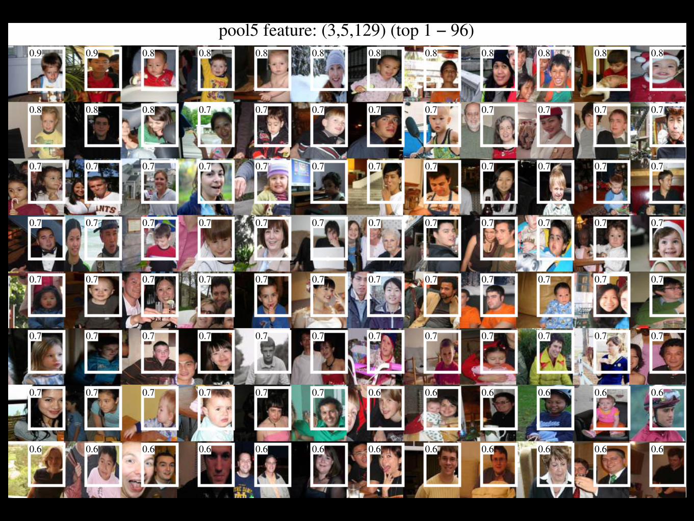
pool5 feature: (3,5,129) (top 1 − 96)0.9 0.9 0.8 0.8 0.8 0.8 0.8 0.8 0.8 0.8 0.8 0.8

0.8 0.8 0.8 0.7 0.7 0.7 0.7 0.7 0.7 0.7 0.7 0.7

0.7 0.7 0.7 0.7 0.7 0.7 0.7 0.7 0.7 0.7 0.7 0.7

0.7 0.7 0.7 0.7 0.7 0.7 0.7 0.7 0.7 0.7 0.7 0.7

0.7 0.7 0.7 0.7 0.7 0.7 0.7 0.7 0.7 0.7 0.7 0.7

0.7 0.7 0.7 0.7 0.7 0.7 0.7 0.7 0.7 0.7 0.7 0.7

0.7 0.7 0.7 0.7 0.7 0.7 0.6 0.6 0.6 0.6 0.6 0.6

0.6 0.6 0.6 0.6 0.6 0.6 0.6 0.6 0.6 0.6 0.6 0.6

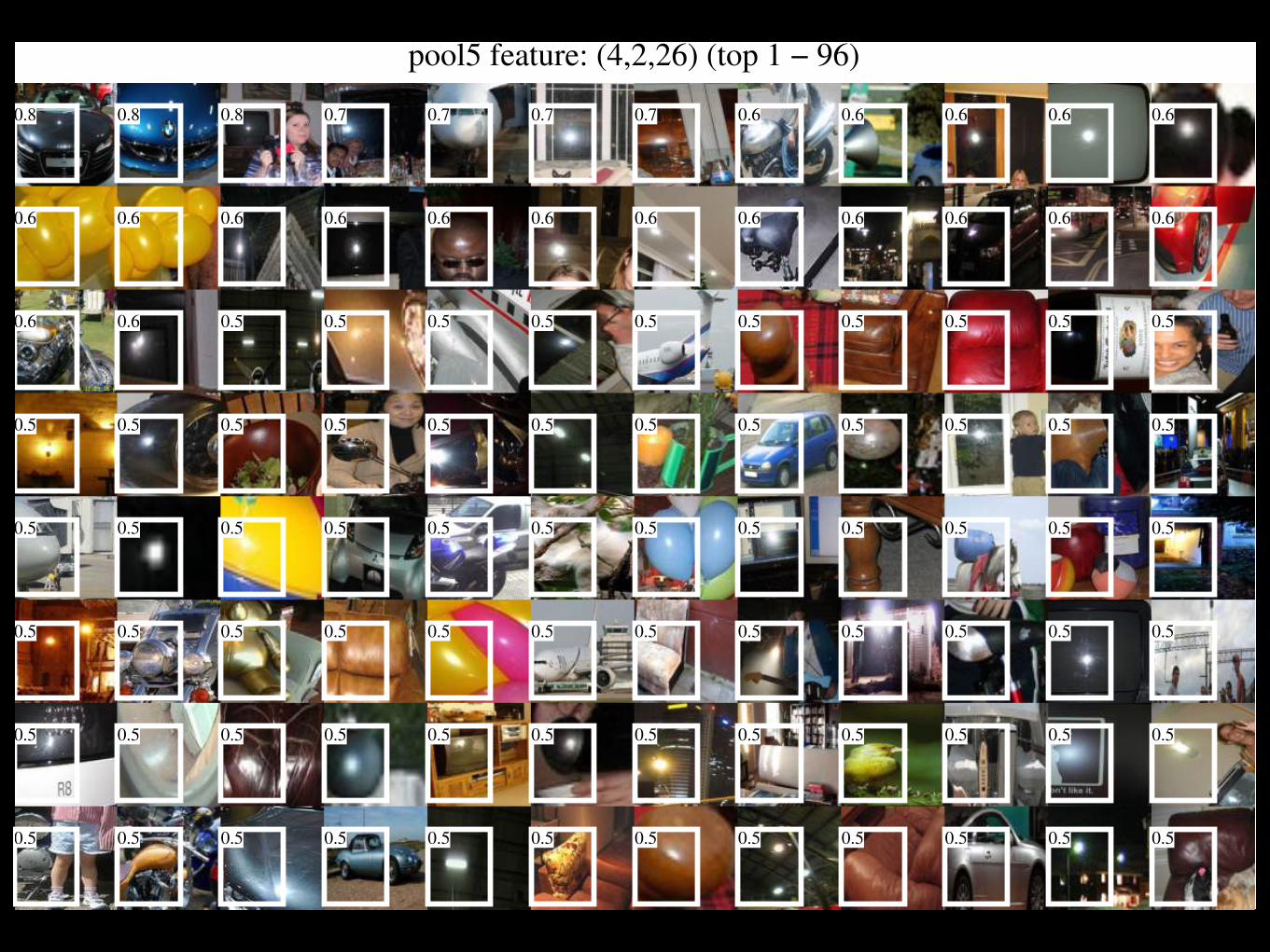
pool5 feature: (4,2,26) (top 1 − 96)

0.8 0.8 0.8 0.7 0.7 0.7 0.7 0.6 0.6 0.6 0.6 0.6

0.6 0.6 0.6 0.6 0.6 0.6 0.6 0.6 0.6 0.6 0.6 0.6

0.6 0.6 0.5 0.5 0.5 0.5 0.5 0.5 0.5 0.5 0.5 0.5

0.5 0.5 0.5 0.5 0.5 0.5 0.5 0.5 0.5 0.5 0.5 0.5

0.5 0.5 0.5 0.5 0.5 0.5 0.5 0.5 0.5 0.5 0.5 0.5

0.5 0.5 0.5 0.5 0.5 0.5 0.5 0.5 0.5 0.5 0.5 0.5

0.5 0.5 0.5 0.5 0.5 0.5 0.5 0.5 0.5 0.5 0.5 0.5

0.5 0.5 0.5 0.5 0.5 0.5 0.5 0.5 0.5 0.5 0.5 0.5

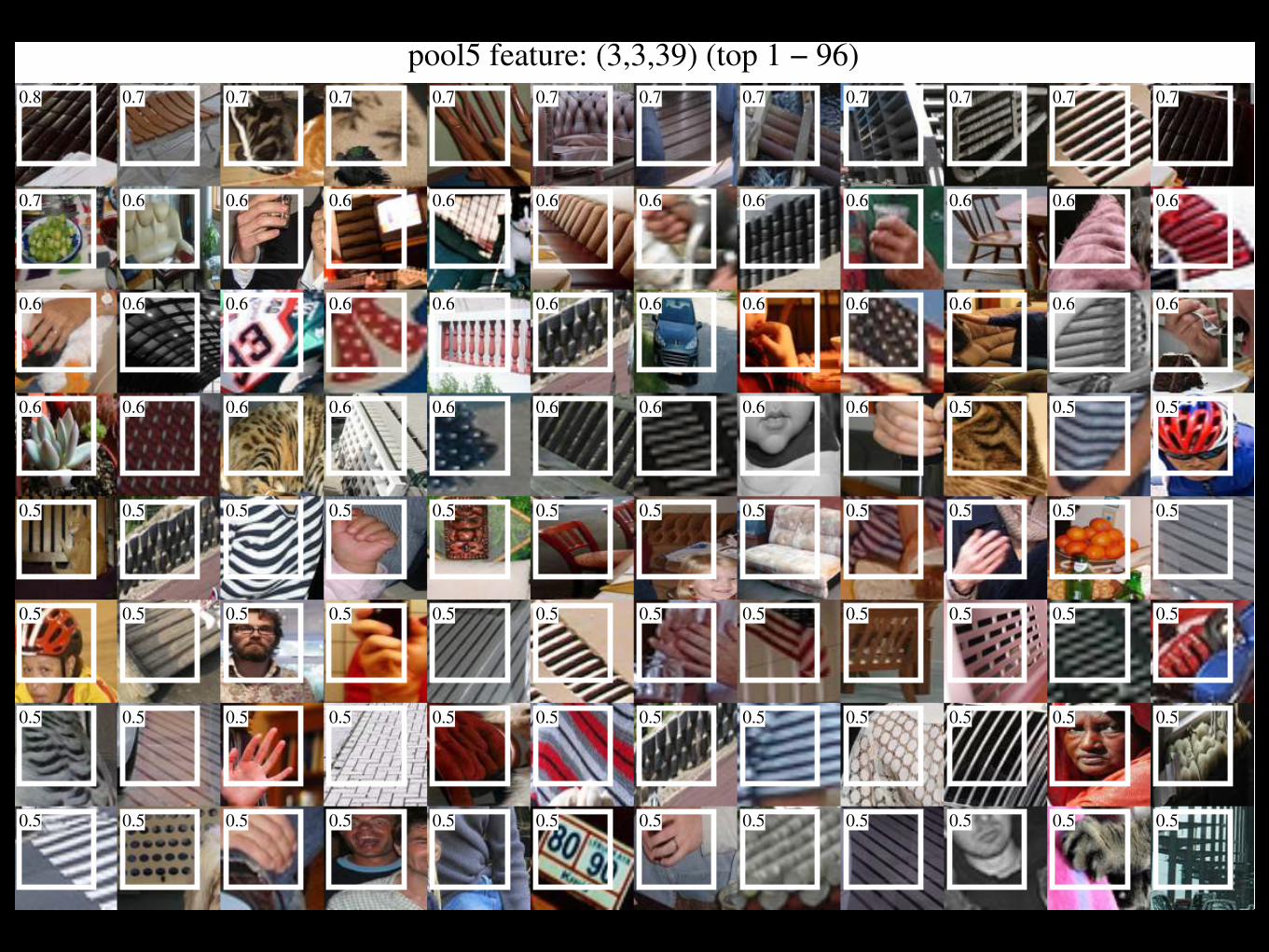
pool5 feature: (3,3,39) (top 1 − 96)0.8 0.7 0.7 0.7 0.7 0.7 0.7 0.7 0.7 0.7 0.7 0.7

0.7 0.6 0.6 0.6 0.6 0.6 0.6 0.6 0.6 0.6 0.6 0.6

0.6 0.6 0.6 0.6 0.6 0.6 0.6 0.6 0.6 0.6 0.6 0.6

0.6 0.6 0.6 0.6 0.6 0.6 0.6 0.6 0.6 0.5 0.5 0.5

0.5 0.5 0.5 0.5 0.5 0.5 0.5 0.5 0.5 0.5 0.5 0.5

0.5 0.5 0.5 0.5 0.5 0.5 0.5 0.5 0.5 0.5 0.5 0.5

0.5 0.5 0.5 0.5 0.5 0.5 0.5 0.5 0.5 0.5 0.5 0.5

0.5 0.5 0.5 0.5 0.5 0.5 0.5 0.5 0.5 0.5 0.5 0.5

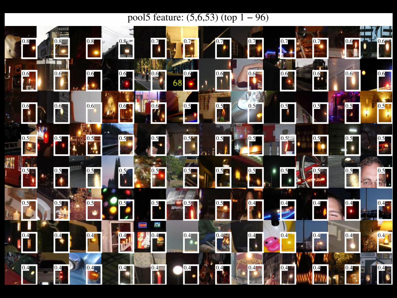
pool5 feature: (5,6,53) (top 1 − 96)

0.8 0.8 0.8 0.8 0.7 0.7 0.7 0.7 0.7 0.7 0.6 0.6

0.6 0.6 0.6 0.6 0.6 0.6 0.6 0.6 0.6 0.6 0.6 0.6

0.6 0.6 0.6 0.6 0.6 0.5 0.5 0.5 0.5 0.5 0.5 0.5

0.5 0.5 0.5 0.5 0.5 0.5 0.5 0.5 0.5 0.5 0.5 0.5

0.5 0.5 0.5 0.5 0.5 0.5 0.5 0.5 0.5 0.5 0.5 0.5

0.5 0.5 0.5 0.5 0.5 0.5 0.5 0.4 0.4 0.4 0.4 0.4

0.4 0.4 0.4 0.4 0.4 0.4 0.4 0.4 0.4 0.4 0.4 0.4

0.4 0.4 0.4 0.4 0.4 0.4 0.4 0.4 0.4 0.4 0.4 0.4

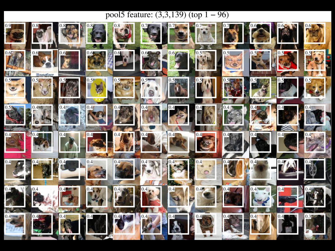
pool5 feature: (3,3,139) (top 1 − 96)0.9 0.8 0.8 0.8 0.8 0.7 0.7 0.7 0.7 0.6 0.6 0.6

0.6 0.6 0.6 0.6 0.6 0.6 0.6 0.5 0.5 0.5 0.5 0.5

0.5 0.5 0.5 0.5 0.5 0.5 0.5 0.5 0.5 0.5 0.5 0.5

0.5 0.4 0.4 0.4 0.4 0.4 0.4 0.4 0.4 0.4 0.4 0.4

0.4 0.4 0.4 0.4 0.4 0.4 0.4 0.4 0.4 0.4 0.4 0.4

0.4 0.4 0.4 0.4 0.4 0.4 0.4 0.4 0.4 0.4 0.4 0.4

0.4 0.4 0.4 0.4 0.4 0.4 0.4 0.4 0.4 0.4 0.4 0.4

0.4 0.4 0.4 0.4 0.4 0.4 0.4 0.4 0.4 0.4 0.4 0.3

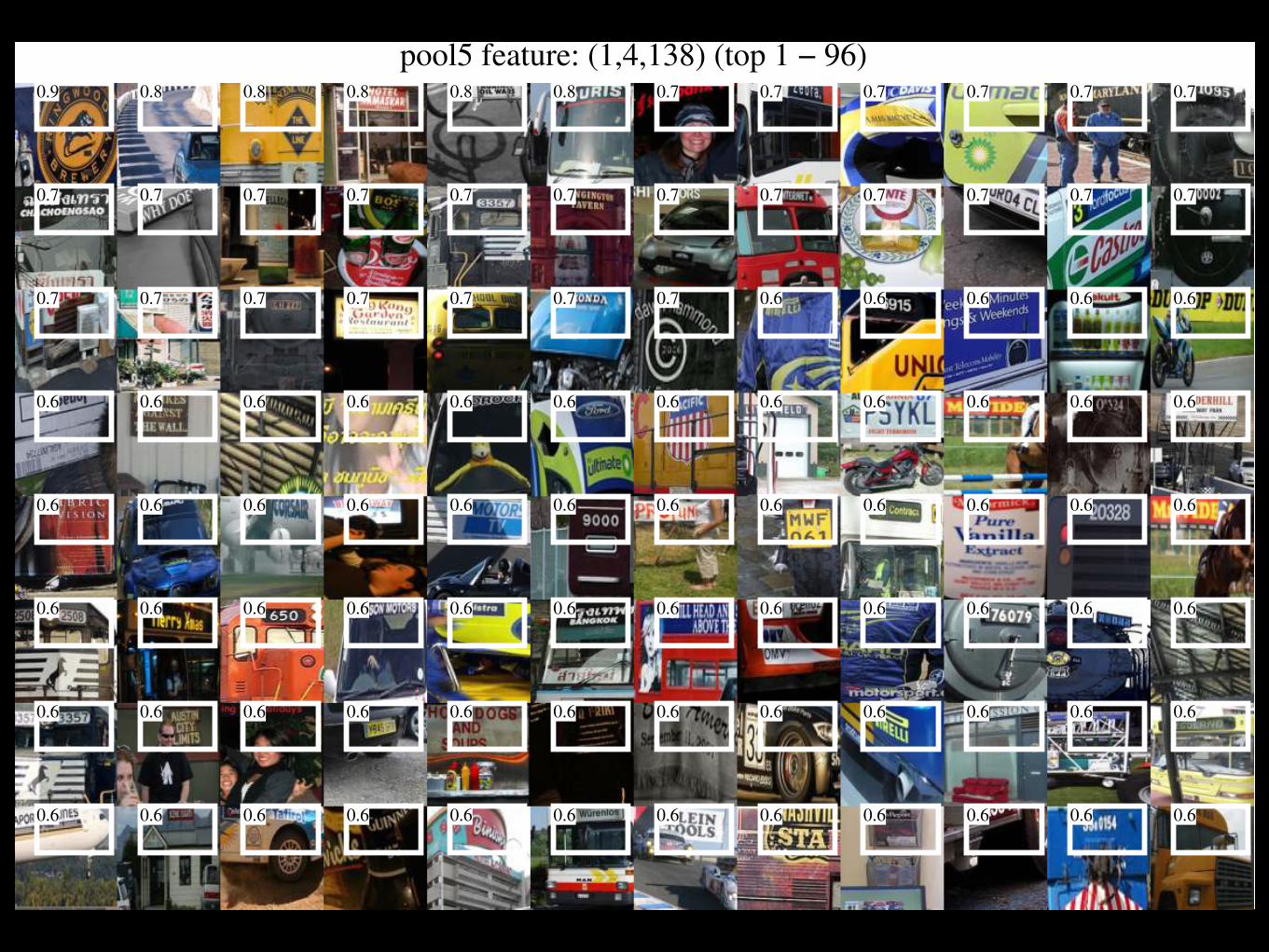
pool5 feature: (1,4,138) (top 1 − 96)0.9 0.8 0.8 0.8 0.8 0.8 0.7 0.7 0.7 0.7 0.7 0.7

0.7 0.7 0.7 0.7 0.7 0.7 0.7 0.7 0.7 0.7 0.7 0.7

0.7 0.7 0.7 0.7 0.7 0.7 0.7 0.6 0.6 0.6 0.6 0.6

0.6 0.6 0.6 0.6 0.6 0.6 0.6 0.6 0.6 0.6 0.6 0.6

0.6 0.6 0.6 0.6 0.6 0.6 0.6 0.6 0.6 0.6 0.6 0.6

0.6 0.6 0.6 0.6 0.6 0.6 0.6 0.6 0.6 0.6 0.6 0.6

0.6 0.6 0.6 0.6 0.6 0.6 0.6 0.6 0.6 0.6 0.6 0.6

0.6 0.6 0.6 0.6 0.6 0.6 0.6 0.6 0.6 0.6 0.6 0.6

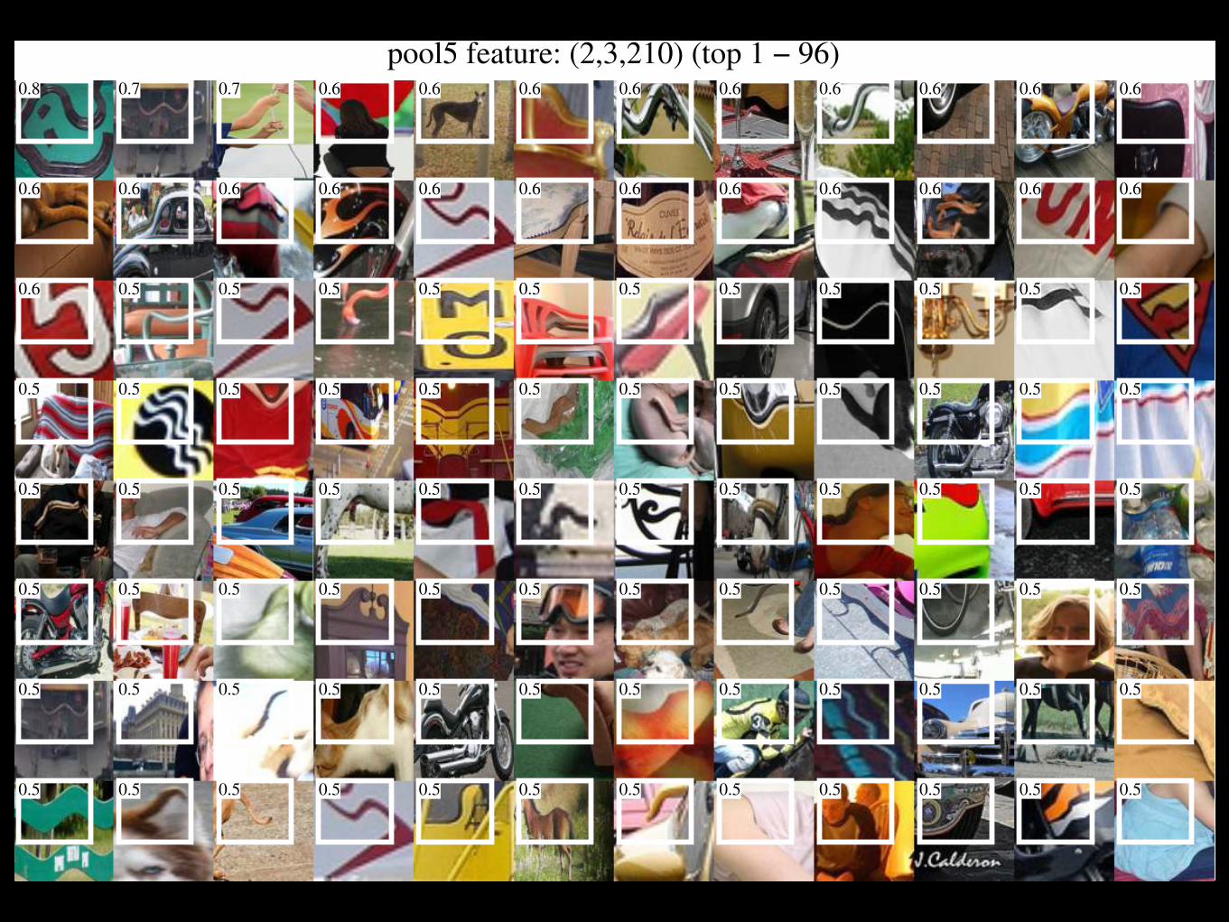
pool5 feature: (2,3,210) (top 1 − 96)0.8 0.7 0.7 0.6 0.6 0.6 0.6 0.6 0.6 0.6 0.6 0.6

0.6 0.6 0.6 0.6 0.6 0.6 0.6 0.6 0.6 0.6 0.6 0.6

0.6 0.5 0.5 0.5 0.5 0.5 0.5 0.5 0.5 0.5 0.5 0.5

0.5 0.5 0.5 0.5 0.5 0.5 0.5 0.5 0.5 0.5 0.5 0.5

0.5 0.5 0.5 0.5 0.5 0.5 0.5 0.5 0.5 0.5 0.5 0.5

0.5 0.5 0.5 0.5 0.5 0.5 0.5 0.5 0.5 0.5 0.5 0.5

0.5 0.5 0.5 0.5 0.5 0.5 0.5 0.5 0.5 0.5 0.5 0.5

0.5 0.5 0.5 0.5 0.5 0.5 0.5 0.5 0.5 0.5 0.5 0.5

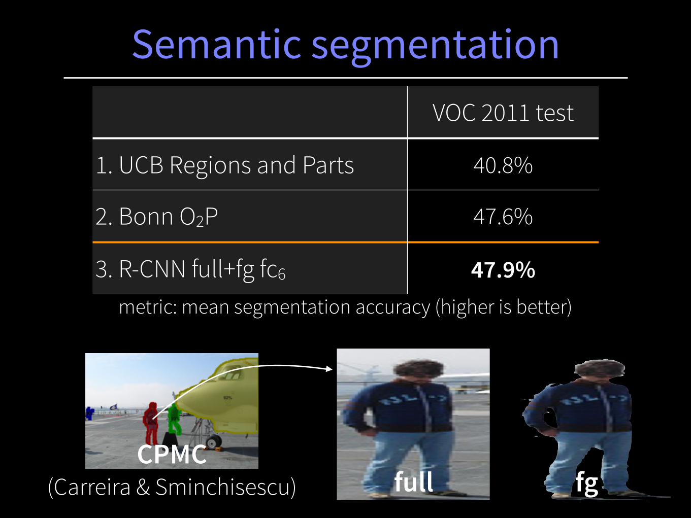
Semantic segmentationVOC 2011 test

1. UCB Regions and Parts 40.8%

2. Bonn O2P 47.6%

3. R-CNN full+fg fc6 47.9%metric: mean segmentation accuracy (higher is better)

full fgCPMC

(Carreira & Sminchisescu)