1

Rheology and structure of COMPLEX FLUIDS

Jan VermantDepartment of Chemical Engineering

K.U. Leuven

Lecturer : Jan Vermant

The material in this lecture is covered by some textbooks, some of them howeverbeing too limited, other ones being probably too detailed. For those among you whowant to know more about rheology we advice the following books:

•Introduction to Rheology (Rheology Series) by H.A. Barnes, J.F. Hutton, K.Walters, Elsevier Science Ltd (1999-2nd edition)•Rheology : Principles, Measurements, and Applications (Advances inInterfacial Engineering) by Christopher W. Macosko, Wiley-VCH (1994)•The Structure and Rheology of Complex Fluids (Topics in ChemicalEngineering) by Ronald G. Larson , Oxford Univ Press (1999)

•For those of you who want to see what is available on the WWW, good startingplaces are:

•The rheology index, a list of rheology related web siteshttp://www.rheology.org/sorindex/default.asp•The European Society of Rheology : http://www.rheology-esr.org/

2

ρειν = flow

Rheology = The Science of Deformation and Flow

1920 : Eugene Bingham (Lafayette College)

Why do we need it?- measure fluid properties- understand structure-property relations- model behaviour- to predict flow behaviour

of complex liquidsunder processing conditions

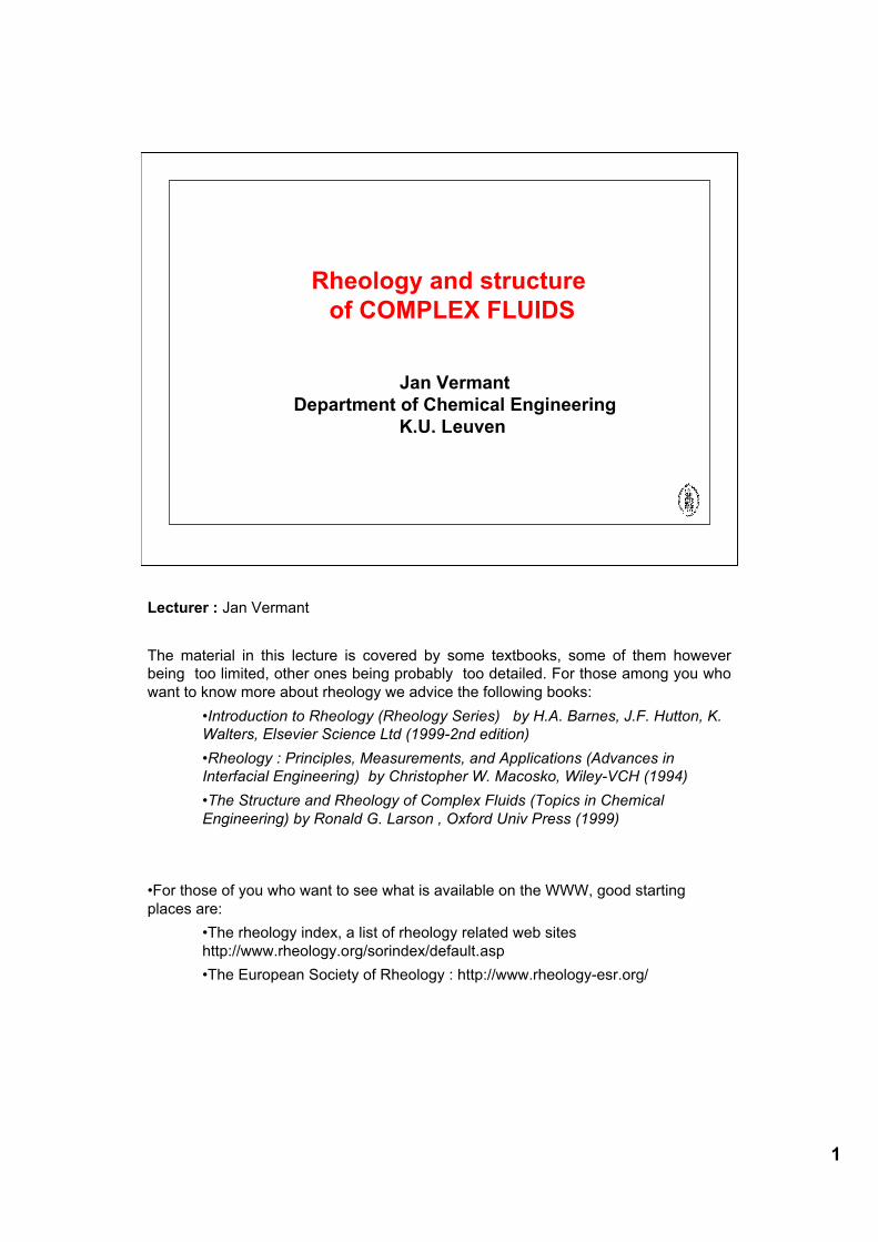
What is Rheology??

Rheology is defined as the science of deformation and flow. In principle, thisdefinition includes everything that deals with flow, such as fluid dynamics, hydraulics,aeronautics and even solid state mechanics. However, in rheology we tend to focuson materials that have a deformation behaviour in between that of liquids and solids,i.e. with a “funny” material behaviors. The science of rheology started in the 1920’swhen polymers started to be produced, leading to novel polymeric substances andnew colloidal fluids (e.g. paints).

Hence the Newtonian fluid and the Hookean elastic solids are outside the scope ofrheology and material behaviour intermediate to these classical extremes will bestudied here. The term “viscoelastic” is used to describe this behavior. Some fluidsare however essentially inelastic, but have a viscosity which changes with thedeformation state, they are called Non-Newtonian fluids.

Rheology is an applied science, and its aim is twofold: Firstly, rheologists try tounderstand the relation between structure and flow properties.This important for theintelligent design and/or formulation of materials for certain applications. Secondly, bystudying the material behavior using simple deformations, fundamental relations willbe derived between deformation and force. Such equations are called constitutiveequations. These equations can then be used to predict the material behavior incomplex deformation histories as they take place in typical process operations: e.g.extrusion, polymer film blowing, spraying, pumping etc.

3

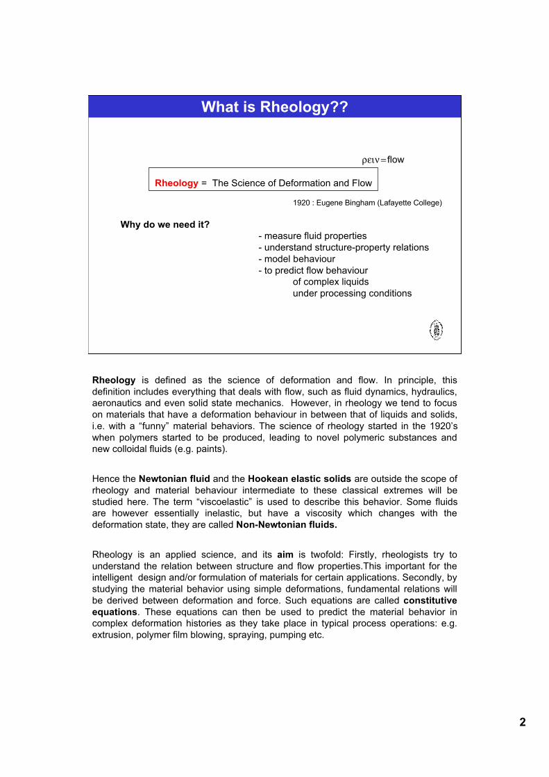
G(t) I - Silly Putty

t < τ t > τ

1. Viscoelasticity

Polydimethylsiloxane + BoraxDr. James Wright, a GE engineer, came upon the material by mixing silicone oil with boric acid.

Peter Hodgson borrowed $147, bought the production rights from GE, and began producing the goo. He renamed it Silly Putty®, and packaged it in plastic eggs because Easter was on the way. Peter Hodgson's product left him an estate of $140 million at his death in 1976.

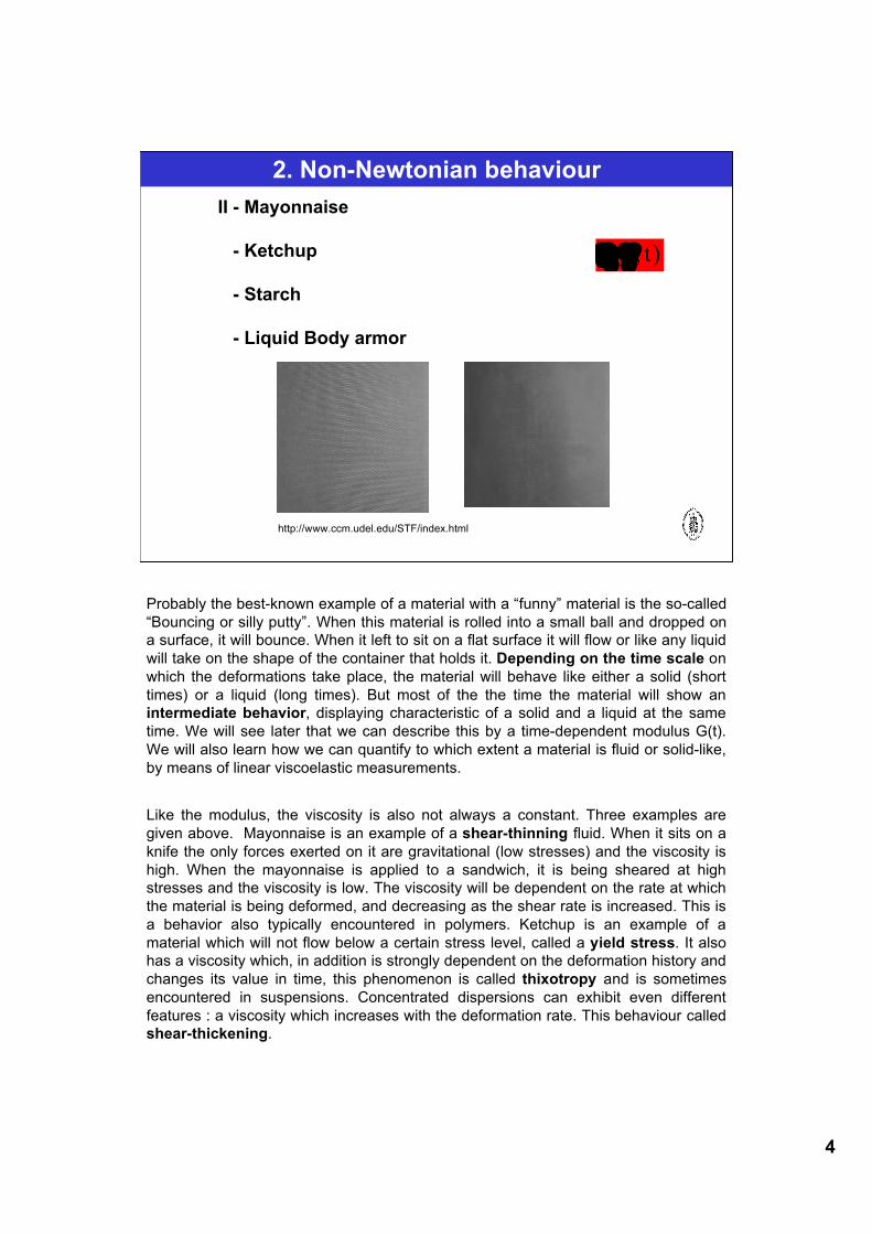
Probably the best-known example of a material with a “funny” material is the so-called“Bouncing or silly putty”. When this material is rolled into a small ball and dropped ona surface, it will bounce. When it left to sit on a flat surface it will flow or like any liquidwill take on the shape of the container that holds it. Depending on the time scale onwhich the deformations take place, the material will behave like either a solid (shorttimes) or a liquid (long times). But most of the the time the material will show anintermediate behavior, displaying characteristic of a solid and a liquid at the sametime. We will see later that we can describe this by a time-dependent modulus G(t).We will also learn how we can quantify to which extent a material is fluid or solid-like,by means of linear viscoelastic measurements.

Like the modulus, the viscosity is also not always a constant. Three examples aregiven above. Mayonnaise is an example of a shear-thinning fluid. When it sits on aknife the only forces exerted on it are gravitational (low stresses) and the viscosity ishigh. When the mayonnaise is applied to a sandwich, it is being sheared at highstresses and the viscosity is low. The viscosity will be dependent on the rate at whichthe material is being deformed, and decreasing as the shear rate is increased. This isa behavior also typically encountered in polymers. Ketchup is an example of amaterial which will not flow below a certain stress level, called a yield stress. It alsohas a viscosity which, in addition is strongly dependent on the deformation history andchanges its value in time, this phenomenon is called thixotropy and is sometimesencountered in suspensions. Concentrated dispersions can exhibit even differentfeatures : a viscosity which increases with the deformation rate. This behaviour calledshear-thickening.

4

II - Mayonnaise

- Ketchup

- Starch

- Liquid Body armor

)t,(!" !

2. Non-Newtonian behaviour

http://www.ccm.udel.edu/STF/index.html

Probably the best-known example of a material with a “funny” material is the so-called“Bouncing or silly putty”. When this material is rolled into a small ball and dropped ona surface, it will bounce. When it left to sit on a flat surface it will flow or like any liquidwill take on the shape of the container that holds it. Depending on the time scale onwhich the deformations take place, the material will behave like either a solid (shorttimes) or a liquid (long times). But most of the the time the material will show anintermediate behavior, displaying characteristic of a solid and a liquid at the sametime. We will see later that we can describe this by a time-dependent modulus G(t).We will also learn how we can quantify to which extent a material is fluid or solid-like,by means of linear viscoelastic measurements.

Like the modulus, the viscosity is also not always a constant. Three examples aregiven above. Mayonnaise is an example of a shear-thinning fluid. When it sits on aknife the only forces exerted on it are gravitational (low stresses) and the viscosity ishigh. When the mayonnaise is applied to a sandwich, it is being sheared at highstresses and the viscosity is low. The viscosity will be dependent on the rate at whichthe material is being deformed, and decreasing as the shear rate is increased. This isa behavior also typically encountered in polymers. Ketchup is an example of amaterial which will not flow below a certain stress level, called a yield stress. It alsohas a viscosity which, in addition is strongly dependent on the deformation history andchanges its value in time, this phenomenon is called thixotropy and is sometimesencountered in suspensions. Concentrated dispersions can exhibit even differentfeatures : a viscosity which increases with the deformation rate. This behaviour calledshear-thickening.

5

III. Weissenberg effect

N1

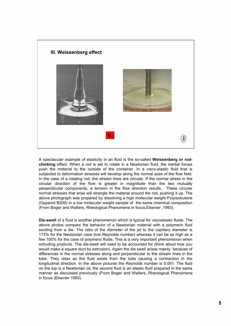
A spectacular example of elasticity in an fluid is the so-called Weissenberg or rod-climbing effect. When a rod is set to rotate in a Newtonian fluid, the inertial forcespush the material to the outside of the container. In a visco-elastic fluid that issubjected to deformation stresses will develop along the normal axes of the flow field.In the case of a rotating rod, the stream lines are circular. If the normal stress in thecircular direction of the flow is greater in magnitude than the two mutuallyperpendicular components, a tension in the flow direction results. These circularnormal stresses that arise will strangle the material around the rod, pushing it up. Theabove photograph was prepared by dissolving a high molecular weight Polyisobutene(Oppanol B200) in a low molecular weight sample of the same chemical composition(From Boger and Walters, Rheological Phenomena in focus,Elsevier ,1993).

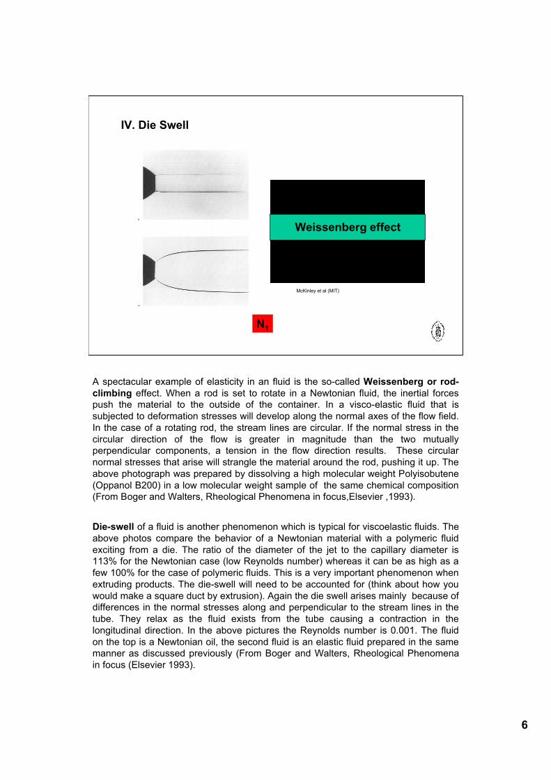
Die-swell of a fluid is another phenomenon which is typical for viscoelastic fluids. Theabove photos compare the behavior of a Newtonian material with a polymeric fluidexciting from a die. The ratio of the diameter of the jet to the capillary diameter is113% for the Newtonian case (low Reynolds number) whereas it can be as high as afew 100% for the case of polymeric fluids. This is a very important phenomenon whenextruding products. The die-swell will need to be accounted for (think about how youwould make a square duct by extrusion). Again the die swell arises mainly because ofdifferences in the normal stresses along and perpendicular to the stream lines in thetube. They relax as the fluid exists from the tube causing a contraction in thelongitudinal direction. In the above pictures the Reynolds number is 0.001. The fluidon the top is a Newtonian oil, the second fluid is an elastic fluid prepared in the samemanner as discussed previously (From Boger and Walters, Rheological Phenomenain focus (Elsevier 1993).

6

IV. Die Swell

N1

Weissenberg effect

McKinley et al (MIT)

A spectacular example of elasticity in an fluid is the so-called Weissenberg or rod-climbing effect. When a rod is set to rotate in a Newtonian fluid, the inertial forcespush the material to the outside of the container. In a visco-elastic fluid that issubjected to deformation stresses will develop along the normal axes of the flow field.In the case of a rotating rod, the stream lines are circular. If the normal stress in thecircular direction of the flow is greater in magnitude than the two mutuallyperpendicular components, a tension in the flow direction results. These circularnormal stresses that arise will strangle the material around the rod, pushing it up. Theabove photograph was prepared by dissolving a high molecular weight Polyisobutene(Oppanol B200) in a low molecular weight sample of the same chemical composition(From Boger and Walters, Rheological Phenomena in focus,Elsevier ,1993).

Die-swell of a fluid is another phenomenon which is typical for viscoelastic fluids. Theabove photos compare the behavior of a Newtonian material with a polymeric fluidexciting from a die. The ratio of the diameter of the jet to the capillary diameter is113% for the Newtonian case (low Reynolds number) whereas it can be as high as afew 100% for the case of polymeric fluids. This is a very important phenomenon whenextruding products. The die-swell will need to be accounted for (think about how youwould make a square duct by extrusion). Again the die swell arises mainly because ofdifferences in the normal stresses along and perpendicular to the stream lines in thetube. They relax as the fluid exists from the tube causing a contraction in thelongitudinal direction. In the above pictures the Reynolds number is 0.001. The fluidon the top is a Newtonian oil, the second fluid is an elastic fluid prepared in the samemanner as discussed previously (From Boger and Walters, Rheological Phenomenain focus (Elsevier 1993).

7

V. Entry flows : vortex enhancement

N1, ηe

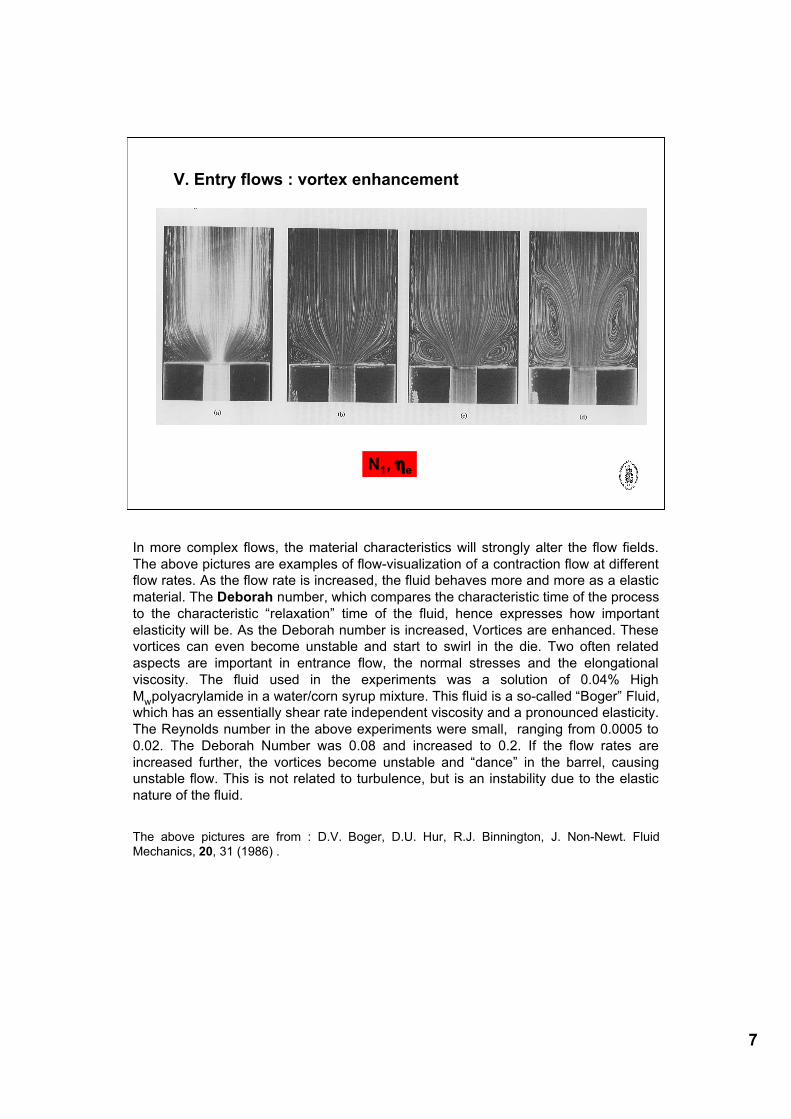
In more complex flows, the material characteristics will strongly alter the flow fields.The above pictures are examples of flow-visualization of a contraction flow at differentflow rates. As the flow rate is increased, the fluid behaves more and more as a elasticmaterial. The Deborah number, which compares the characteristic time of the processto the characteristic “relaxation” time of the fluid, hence expresses how importantelasticity will be. As the Deborah number is increased, Vortices are enhanced. Thesevortices can even become unstable and start to swirl in the die. Two often relatedaspects are important in entrance flow, the normal stresses and the elongationalviscosity. The fluid used in the experiments was a solution of 0.04% HighMwpolyacrylamide in a water/corn syrup mixture. This fluid is a so-called “Boger” Fluid,which has an essentially shear rate independent viscosity and a pronounced elasticity.The Reynolds number in the above experiments were small, ranging from 0.0005 to0.02. The Deborah Number was 0.08 and increased to 0.2. If the flow rates areincreased further, the vortices become unstable and “dance” in the barrel, causingunstable flow. This is not related to turbulence, but is an instability due to the elasticnature of the fluid.

The above pictures are from : D.V. Boger, D.U. Hur, R.J. Binnington, J. Non-Newt. FluidMechanics, 20, 31 (1986) .

8

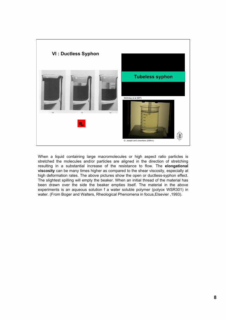
VI : Ductless Syphon

ηe

Tubeless syphon

McKinley et al (MIT)

D. Joseph and coworkers (UMinn)

When a liquid containing large macromolecules or high aspect ratio particles isstretched the molecules and/or particles are aligned in the direction of stretchingresulting in a substantial increase of the resistance to flow. The elongationalviscosity can be many times higher as compared to the shear viscosity, especially athigh deformation rates. The above pictures show the open or ductless-syphon effect.The slightest spilling will empty the beaker. When an initial thread of the material hasbeen drawn over the side the beaker empties itself. The material in the aboveexperiments is an aqueous solution f a water soluble polymer (polyox WSR301) inwater. (From Boger and Walters, Rheological Phenomena in focus,Elsevier ,1993).

9

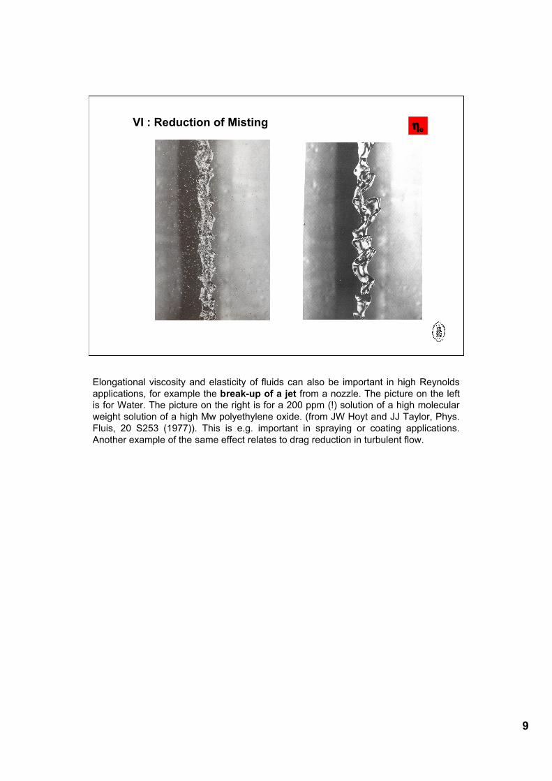
VI : Reduction of Misting ηe

Elongational viscosity and elasticity of fluids can also be important in high Reynoldsapplications, for example the break-up of a jet from a nozzle. The picture on the leftis for Water. The picture on the right is for a 200 ppm (!) solution of a high molecularweight solution of a high Mw polyethylene oxide. (from JW Hoyt and JJ Taylor, Phys.Fluis, 20 S253 (1977)). This is e.g. important in spraying or coating applications.Another example of the same effect relates to drag reduction in turbulent flow.

10

Aim of this lecture:

1. Qualitative insight of the behavior of non-Newtonian fluids.

2. Discuss measurement techniques for a given problem

3. Demonstrate link rheological properties // microstructure

11

Rheology

Finite Deformation Tensors

We now have a way to determine the state of stress in a material. Now we need asimilar three-dimensional description of the state of deformation in a material. Relatingstresses and deformations leads us to the constitutive equations that we are lookingfor. How do we proceed? Do we look to describe all the velocities in a fluid? This is ofnot much use (fortunately)- we need the relative deformations.

At the end of this session we should have a description for:- deformations (relative)- deformation gradients

Let’s keep this in mind:If we write Hooke’s law in three dimensions, with the stress and strain beingproportional, the deformations tensors should be such that rotations do not give rise toa stress. Likewise we will try to see if we can write Newton’s law in three dimensions.

12

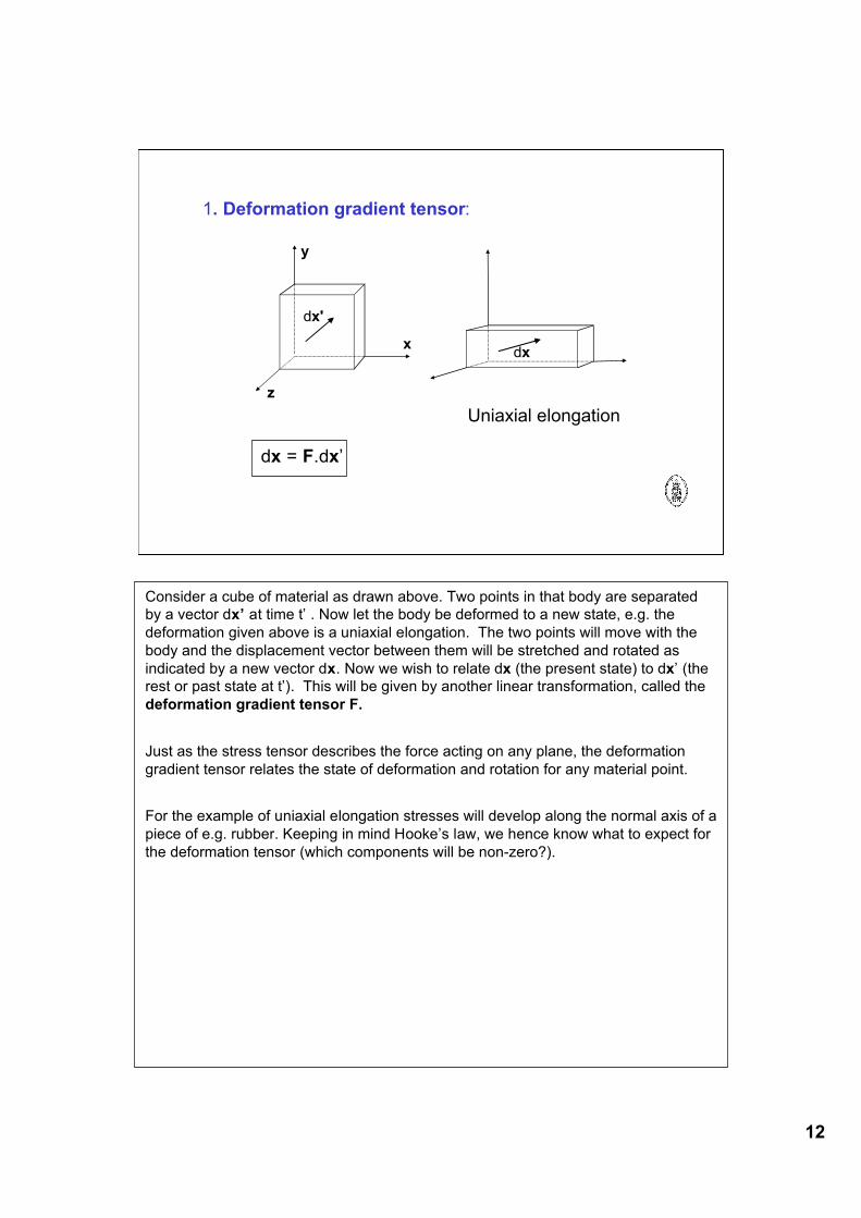
1. Deformation gradient tensor:

y

x

z

dx'

dx

dx = F.dx’

Uniaxial elongation

Consider a cube of material as drawn above. Two points in that body are separatedby a vector dx’ at time t’ . Now let the body be deformed to a new state, e.g. thedeformation given above is a uniaxial elongation. The two points will move with thebody and the displacement vector between them will be stretched and rotated asindicated by a new vector dx. Now we wish to relate dx (the present state) to dx’ (therest or past state at t’). This will be given by another linear transformation, called thedeformation gradient tensor F.

Just as the stress tensor describes the force acting on any plane, the deformationgradient tensor relates the state of deformation and rotation for any material point.

For the example of uniaxial elongation stresses will develop along the normal axis of apiece of e.g. rubber. Keeping in mind Hooke’s law, we hence know what to expect forthe deformation tensor (which components will be non-zero?).

13

S

h

! = s/h

"

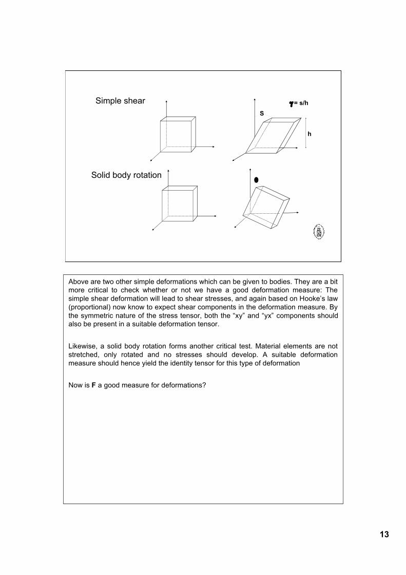
Simple shear

Solid body rotation

Above are two other simple deformations which can be given to bodies. They are a bitmore critical to check whether or not we have a good deformation measure: Thesimple shear deformation will lead to shear stresses, and again based on Hooke’s law(proportional) now know to expect shear components in the deformation measure. Bythe symmetric nature of the stress tensor, both the “xy” and “yx” components shouldalso be present in a suitable deformation tensor.

Likewise, a solid body rotation forms another critical test. Material elements are notstretched, only rotated and no stresses should develop. A suitable deformationmeasure should hence yield the identity tensor for this type of deformation

Now is F a good measure for deformations?

14

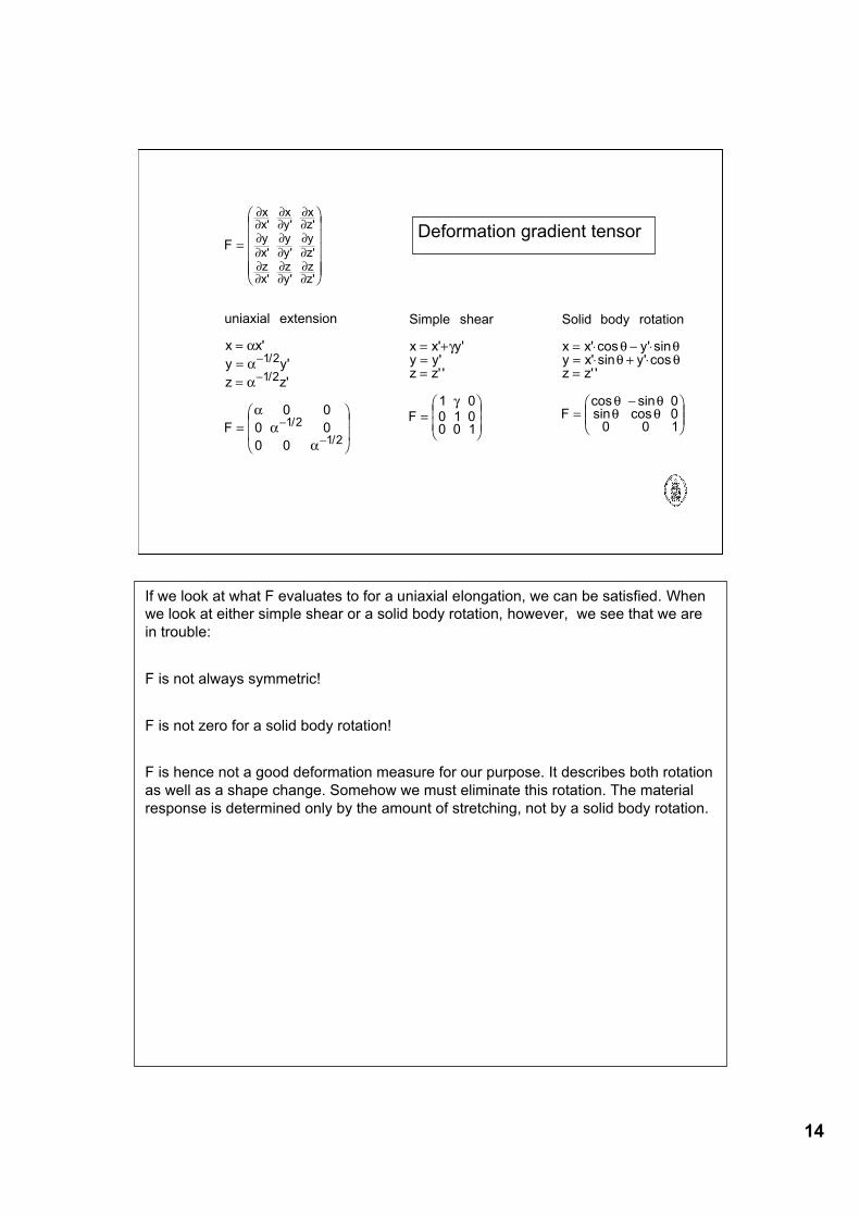
F

uniaxial extension

x x

y y

z z

F

xx

xy

xz

y

x

y

y

y

zzx

zy

zz

=

!

"

#####

$

%

&&&&&

=

=

=

=

!

"

##

$

%

&&

'

'

''

((

((

((

((

((

((

((

((

((

)))

))

)

' ' '

' ' '

' ' '

/

/

/

/

'

'

'

1 2

1 2

1 2

1 2

0 0

0 0

0 0

Deformation gradient tensor

Simple shear

x x yy yz z

F

= +

=

=

=

!

"##

$

%&&

' ''' '

'

'1 00 1 00 0 1

Solid body rotation

x x yy x yz z

F

= ! " != ! + !=

=

"#

$%%

&

'((

' cos ' sin' sin ' cos' '

cos sinsin cos

) )) )

) )) )

00

0 0 1

If we look at what F evaluates to for a uniaxial elongation, we can be satisfied. Whenwe look at either simple shear or a solid body rotation, however, we see that we arein trouble:

F is not always symmetric!

F is not zero for a solid body rotation!

F is hence not a good deformation measure for our purpose. It describes both rotationas well as a shape change. Somehow we must eliminate this rotation. The materialresponse is determined only by the amount of stretching, not by a solid body rotation.

15

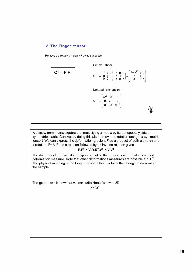
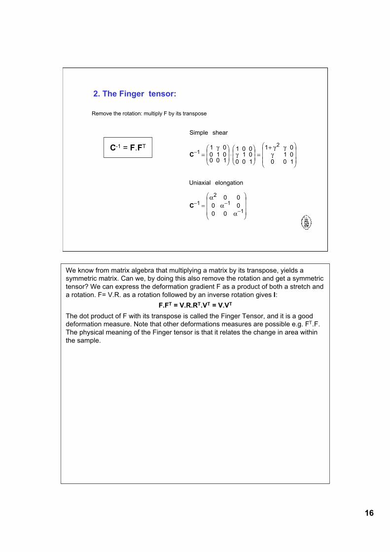
2. The Finger tensor:

Remove the rotation: multiply F by its transpose

C-1 = F.FT

Simple shear

1 00 1 00 0 1

1 0 01 0

0 0 1

1 01 0

0 0 1

Uniaxial elongation

0 0

0 0

0 0

1

2

1

2

1

1

C

C

!

! !!

=

"

#$$

%

&''("

#$$

%

&'' =

+"

#

$$$

%

&

'''

=

"

#

$$$

%

&

'''

))

) ))

**

*

We know from matrix algebra that multiplying a matrix by its transpose, yields asymmetric matrix. Can we, by doing this also remove the rotation and get a symmetrictensor? We can express the deformation gradient F as a product of both a stretch anda rotation. F= V.R. as a rotation followed by an inverse rotation gives I:

F.FT = V.R.RT.VT = V.VT

The dot product of F with its transpose is called the Finger Tensor, and it is a gooddeformation measure. Note that other deformations measures are possible e.g. FT.F.The physical meaning of the Finger tensor is that it relates the change in area withinthe sample.

The good news is now that we can write Hooke’s law in 3D!σ=GC-1

16

2. The Finger tensor:

Remove the rotation: multiply F by its transpose

C-1 = F.FT

Simple shear

1 00 1 00 0 1

1 0 01 0

0 0 1

1 01 0

0 0 1

Uniaxial elongation

0 0

0 0

0 0

1

2

1

2

1

1

C

C

!

! !!

=

"

#$$

%

&''("

#$$

%

&'' =

+"

#

$$$

%

&

'''

=

"

#

$$$

%

&

'''

))

) ))

**

*

We know from matrix algebra that multiplying a matrix by its transpose, yields asymmetric matrix. Can we, by doing this also remove the rotation and get a symmetrictensor? We can express the deformation gradient F as a product of both a stretch anda rotation. F= V.R. as a rotation followed by an inverse rotation gives I:

F.FT = V.R.RT.VT = V.VT

The dot product of F with its transpose is called the Finger Tensor, and it is a gooddeformation measure. Note that other deformations measures are possible e.g. FT.F.The physical meaning of the Finger tensor is that it relates the change in area withinthe sample.

17

3. Neo-Hookean Solid:

Using the Finger tensor we can come up with a general form of Hooke’s law

σ = G . C-1

Simple shear

! = G.C"1=

1 # 0

0 1 0

0 0 1

$

%

&&

'

(

))*

1 0 0

# 1 0

0 0 1

$

%

&&

'

(

))= G.

1+ # 2 # 0

# 1 0

0 0 1

$

%

&&&

'

(

)))

! xy = G#

Uniaxial elongation

! = G.C"1= G.

+ 2 0 0

0 +"1 0

0 0 +"1

$

%

&&&

'

(

)))

! xx = " p +G+ 2=

G

1+ ,"G(1+ ,)2

= G3, + 3, 2

+ , 3

1+ ,- 3,G = E,

The good news is now that we can write Hooke’s law in 3D!σ=GC-1

Actually Hooke observed the proportionality between force and stress for “a springybody” as early as 1678 and it took almost 150 years to formulate this model in 3D.

For an incompressible solid, the above calculation shows the link between the shearmodulus G and Young’s modulus E. For compressible materials, a Poisson-coefficientneeds to be used. For more details we refer to the textbook by Macosko or the course “Sterkteleer”.

18

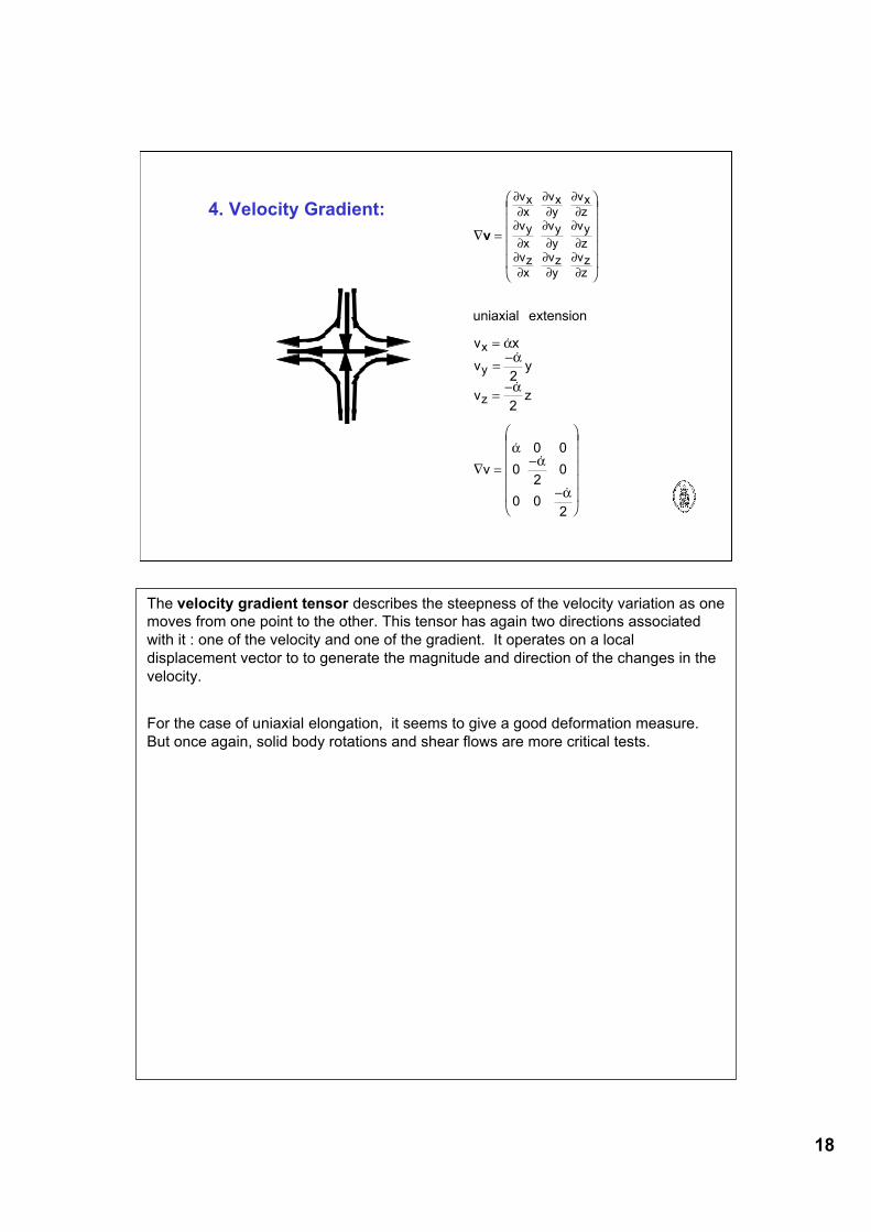
4. Velocity Gradient:! =

"

#

$$$$$

%

&

'''''

=

=(

=(

! =(

(

"

#

$$$$$

%

&

'''''

v

))

))

))

))

))

))

))

))

))

**

*

**

*

vxx

vxy

vxz

vy

x

vy

y

vy

zvzx

vzy

vzz

x

y

z

uniaxial extension

v x

v2y

v2z

v

0 0

02

0

0 02

!

!

!

!

!

!

The velocity gradient tensor describes the steepness of the velocity variation as onemoves from one point to the other. This tensor has again two directions associatedwith it : one of the velocity and one of the gradient. It operates on a localdisplacement vector to to generate the magnitude and direction of the changes in thevelocity.

For the case of uniaxial elongation, it seems to give a good deformation measure.But once again, solid body rotations and shear flows are more critical tests.

19

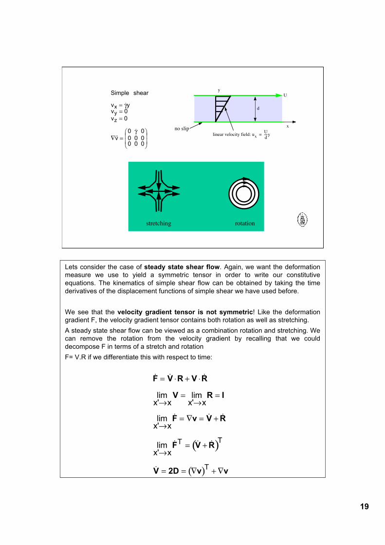
Simple shear

v yv

v

v

xy

z

=

=

=

! =

"

#$$

%

&''

!

!

(

(

0

0

0 00 0 00 0 0

"

U

d

no slipx

y

linear velocity field: uxU

d----y=

stretching rotation

Lets consider the case of steady state shear flow. Again, we want the deformationmeasure we use to yield a symmetric tensor in order to write our constitutiveequations. The kinematics of simple shear flow can be obtained by taking the timederivatives of the displacement functions of simple shear we have used before.

We see that the velocity gradient tensor is not symmetric! Like the deformationgradient F, the velocity gradient tensor contains both rotation as well as stretching.A steady state shear flow can be viewed as a combination rotation and stretching. Wecan remove the rotation from the velocity gradient by recalling that we coulddecompose F in terms of a stretch and rotationF= V.R if we differentiate this with respect to time:

( )

( )

! ! !

lim'

lim'

lim'

! ! !

lim'

! ! !

!

F V R V R

V R I

F v V R

F V R

V 2D v v

= ! + !

"=

"=

"= # = +

"= +

= = # +#

x x x x

x x

x x

T T

T

20

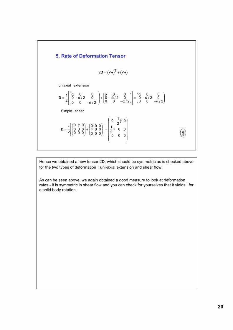
5. Rate of Deformation Tensor

( ) ( )2D v v= ! + !T

Simple shear

0 0

0 0 00 0 0

0 00 0

0 0 0

0 0

0 0

0 0 0

D =

!

"##

$

%&&+

!

"##

$

%&&

'

(

))

*

+

,,=

!

"

######

$

%

&&&&&&

1

2

0

1

21

2

!

!

!

!

--

-

-

uniaxial extension

0 0

0 0

0 0

0 0

0 0

0 0

0 0

0 0

0 0

D = !!

"

#

$$

%

&

'' + !

!

"

#$$

%

&''

(

)

**

+

,

--= !

!

"

#$$

%

&''

1

22

2

2

2

2

2

!

! /

! /

!

! /! /

!

! /! /

..

.

..

.

..

.

Hence we obtained a new tensor 2D, which should be symmetric as is checked abovefor the two types of deformation : uni-axial extension and shear flow.

As can be seen above, we again obtained a good measure to look at deformationrates - it is symmetric in shear flow and you can check for yourselves that it yields I fora solid body rotation.

21

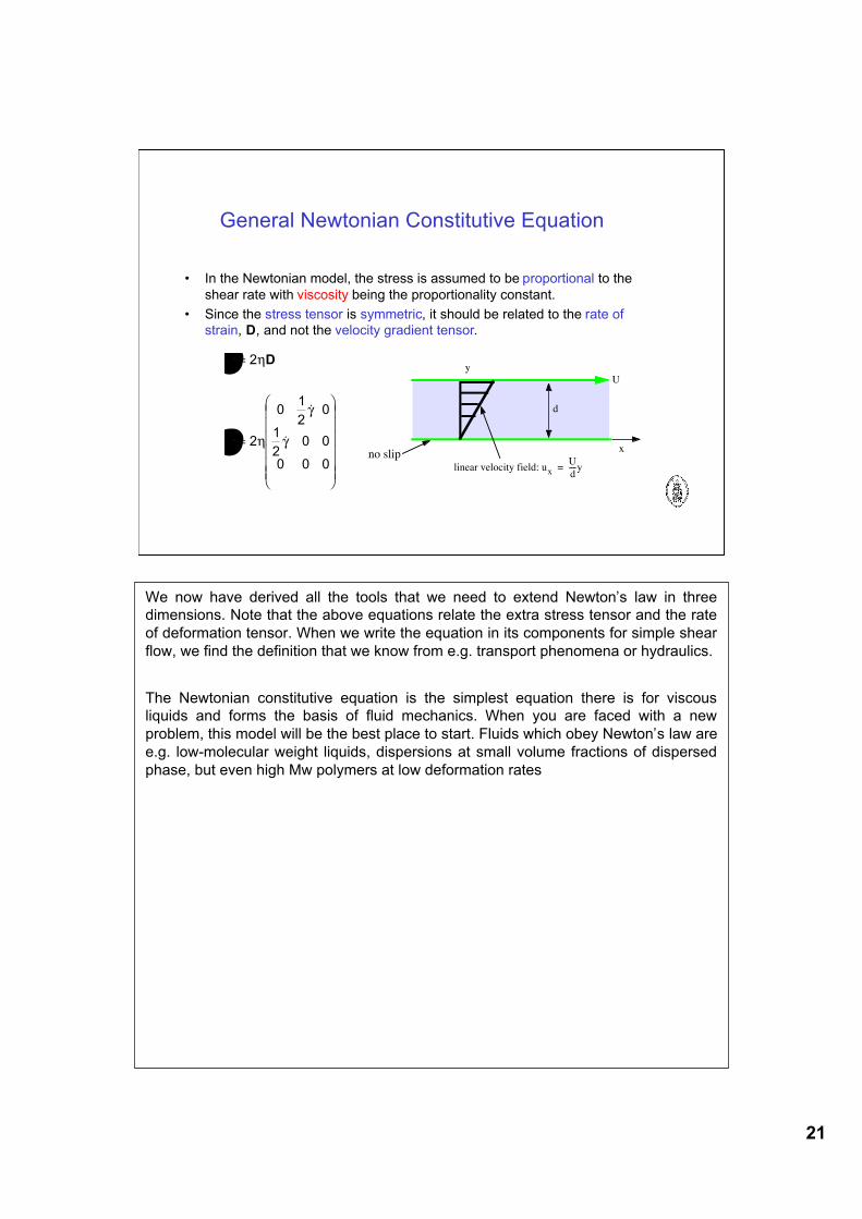
General Newtonian Constitutive Equation

• In the Newtonian model, the stress is assumed to be proportional to theshear rate with viscosity being the proportionality constant.

• Since the stress tensor is symmetric, it should be related to the rate ofstrain, D, and not the velocity gradient tensor.

!

!

=

=

"

#

$$$$$$

%

&

''''''

2

2

01

20

1

20 0

0 0 0

(

(

)

)

D

!

!

U

d

no slipx

y

linear velocity field: uxU

d----y=

We now have derived all the tools that we need to extend Newton’s law in threedimensions. Note that the above equations relate the extra stress tensor and the rateof deformation tensor. When we write the equation in its components for simple shearflow, we find the definition that we know from e.g. transport phenomena or hydraulics.

The Newtonian constitutive equation is the simplest equation there is for viscousliquids and forms the basis of fluid mechanics. When you are faced with a newproblem, this model will be the best place to start. Fluids which obey Newton’s law aree.g. low-molecular weight liquids, dispersions at small volume fractions of dispersedphase, but even high Mw polymers at low deformation rates

22

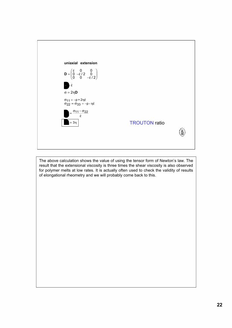
uniaxial extension

D

D

= !!

"

#$$

%

&''

=

=

=

=!

=

= != !

!

! /! /

! !

!

!

!

((

(

(

) *

) () ) (

) )(

**

*

0 00 00 0

p+ 2

p -

e

e 3

22

2

11

22 33

11 22

+

*

* TROUTON ratio

The above calculation shows the value of using the tensor form of Newton’s law. Theresult that the extensional viscosity is three times the shear viscosity is also observedfor polymer melts at low rates. It is actually often used to check the validity of resultsof elongational rheometry and we will probably come back to this.

23

Linear Viscoelasticity

In this chapter we will see one of the most important aspects of rheology: the description of linearviscoelasticity. Linear viscoelasticity is important for a number of reasons:

It is an important goal of rheology that we are able to describe and characterize materialbehavior that is intermediate between solid and liquid behaviour. The linear regime is important because it is the building block for further work: howcomplicated the non-linear regime might be, we should always find the linear viscoelasticbehavior as a limiting case. Last but not least linear viscoelasticity is of practical importance: For example for linearpolymer chains, measurements characterizing the linear viscoelastic properties provide insight into how the material will behave in some non-linear flows.

At the end of this chapter you should be able to:• define linear viscoelasticity.• understand it from an energetical point of view.• be able to describe linear viscoelasticity mathematically• know which properties can be determined experimentally and how they are interrelated :relaxation modulus, compliance, storage and loss modulus and relaxation spectrum

24

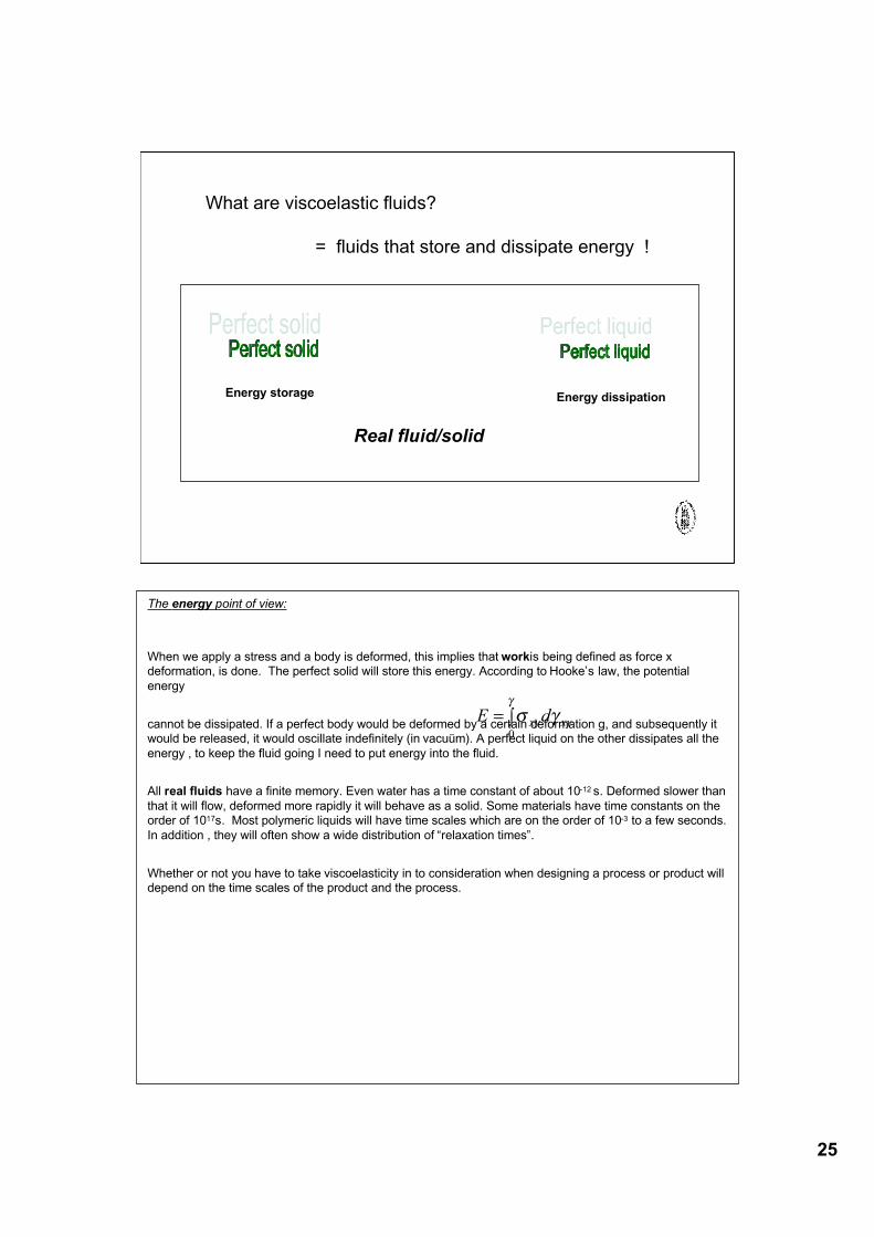
What are viscoelastic fluids?

= fluids with a finite memory !

Memory = ∞ Memory = 0

Real fluid/solid

The memory point of view:

Viscoelastic fluids are defined as fluids which have a finite memory. The two materialclasses we have worked with up to now; the perfect solid (Hooke’s law) and theperfect liquid (Newton’s law) do not obey this definition. A perfect solid will rememberthe deformation indefinitely and return to its initial shape. A perfect liquid will stopdeforming instantaneously when the stress is removed and never recover to itsprevious shape.

All real fluids and solids show intermediate behavior. I cannot recuperate the energythat I put into a deformed solid. There will always be some internal dissipation ofenergy. For example car tyres heat up during driving, not soo much due to the friction,but due to the internal heat dissipation.

25

What are viscoelastic fluids?

= fluids that store and dissipate energy !

Energy storage Energy dissipation

Real fluid/solid

The energy point of view:

When we apply a stress and a body is deformed, this implies that workis being defined as force xdeformation, is done. The perfect solid will store this energy. According to Hooke’s law, the potentialenergy

cannot be dissipated. If a perfect body would be deformed by a certain deformation g, and subsequently itwould be released, it would oscillate indefinitely (in vacuüm). A perfect liquid on the other dissipates all theenergy , to keep the fluid going I need to put energy into the fluid.

All real fluids have a finite memory. Even water has a time constant of about 10-12 s. Deformed slower thanthat it will flow, deformed more rapidly it will behave as a solid. Some materials have time constants on theorder of 1017s. Most polymeric liquids will have time scales which are on the order of 10-3 to a few seconds.In addition , they will often show a wide distribution of “relaxation times”.

Whether or not you have to take viscoelasticity in to consideration when designing a process or product willdepend on the time scales of the product and the process.

!=

""#

0

xyxydE

26

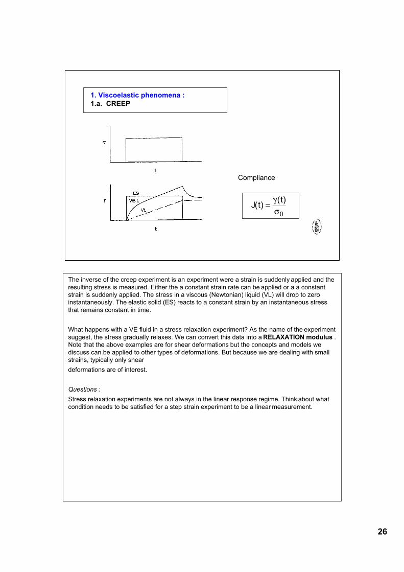
1. Viscoelastic phenomena :1.a. CREEP

Compliance

J tt

( )( )

=!

"0

The inverse of the creep experiment is an experiment were a strain is suddenly applied and theresulting stress is measured. Either the a constant strain rate can be applied or a a constantstrain is suddenly applied. The stress in a viscous (Newtonian) liquid (VL) will drop to zeroinstantaneously. The elastic solid (ES) reacts to a constant strain by an instantaneous stressthat remains constant in time.

What happens with a VE fluid in a stress relaxation experiment? As the name of the experimentsuggest, the stress gradually relaxes. We can convert this data into a RELAXATION modulus .Note that the above examples are for shear deformations but the concepts and models wediscuss can be applied to other types of deformations. But because we are dealing with smallstrains, typically only sheardeformations are of interest.

Questions :Stress relaxation experiments are not always in the linear response regime. Think about whatcondition needs to be satisfied for a step strain experiment to be a linear measurement.

27

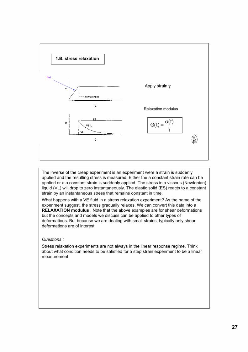
1.B. stress relaxation

G tt

( )( )

=!

"

Relaxation modulus

fast

Apply strain γ

The inverse of the creep experiment is an experiment were a strain is suddenlyapplied and the resulting stress is measured. Either the a constant strain rate can beapplied or a a constant strain is suddenly applied. The stress in a viscous (Newtonian)liquid (VL) will drop to zero instantaneously. The elastic solid (ES) reacts to a constantstrain by an instantaneous stress that remains constant in time.What happens with a VE fluid in a stress relaxation experiment? As the name of theexperiment suggest, the stress gradually relaxes. We can convert this data into aRELAXATION modulus . Note that the above examples are for shear deformationsbut the concepts and models we discuss can be applied to other types ofdeformations. But because we are dealing with small strains, typically only sheardeformations are of interest.

Questions :Stress relaxation experiments are not always in the linear response regime. Thinkabout what condition needs to be satisfied for a step strain experiment to be a linearmeasurement.

28

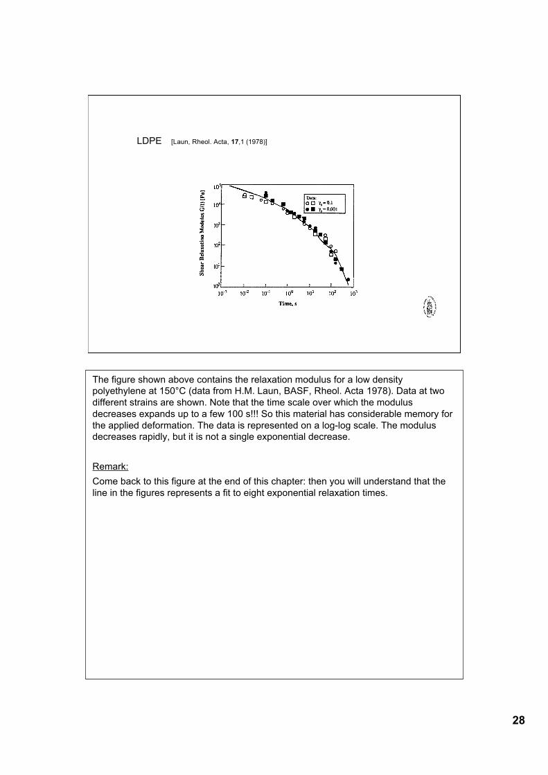
LDPE [Laun, Rheol. Acta, 17,1 (1978)]

The figure shown above contains the relaxation modulus for a low densitypolyethylene at 150°C (data from H.M. Laun, BASF, Rheol. Acta 1978). Data at twodifferent strains are shown. Note that the time scale over which the modulusdecreases expands up to a few 100 s!!! So this material has considerable memory forthe applied deformation. The data is represented on a log-log scale. The modulusdecreases rapidly, but it is not a single exponential decrease.

Remark:Come back to this figure at the end of this chapter: then you will understand that theline in the figures represents a fit to eight exponential relaxation times.

29

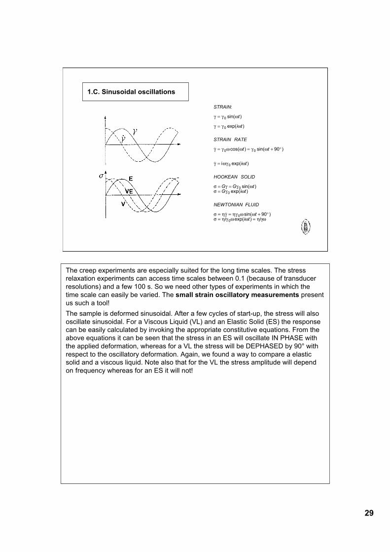
1.C. Sinusoidal oscillations

STRAIN

t

i t

STRAIN RATE

t t

i t

HOOKEAN SOLID

G G t

G i t

NEWTONIAN FLUID

t

i i t i

:

sin( )

exp( )

! cos( ) sin( )

! i exp( )

sin( )exp( )

! sin( )exp( )

! ! "

! ! "

! ! " " ! "

! "! "

# ! ! "# ! "

# $! $! " "# $ ! " " $ !"

=

=

= = + °

=

= =

=

= = + °

= =

0

0

0 0

0

0

0

0

0

90

90

The creep experiments are especially suited for the long time scales. The stressrelaxation experiments can access time scales between 0.1 (because of transducerresolutions) and a few 100 s. So we need other types of experiments in which thetime scale can easily be varied. The small strain oscillatory measurements presentus such a tool!The sample is deformed sinusoidal. After a few cycles of start-up, the stress will alsooscillate sinusoidal. For a Viscous Liquid (VL) and an Elastic Solid (ES) the responsecan be easily calculated by invoking the appropriate constitutive equations. From theabove equations it can be seen that the stress in an ES will oscillate IN PHASE withthe applied deformation, whereas for a VL the stress will be DEPHASED by 90° withrespect to the oscillatory deformation. Again, we found a way to compare a elasticsolid and a viscous liquid. Note also that for the VL the stress amplitude will dependon frequency whereas for an ES it will not!

30

[ ]

( ) ( )

[ ]

VISCOELASTIC MATERIAL

t

i t

complex ulus

G

G t

G t t

G t G t

G t G t

G iG

! ! " #

! ! " #

! $

! $ " #

! $ " # " #

! # $ " # $ "

! " " $

! $

= +

= +

=

= +

= +

= % + %

= % + %

= +

&

&

&

& &

0

0

0

0

0 0

0

sin( )

exp( )

mod :

sin( )

sin( ).cos( ) cos( ).sin( )

cos( ) sin( ) sin( ) cos( )

' sin( ) " cos( )

( ' " )

Storage and Loss modulus'

''tan

G

G=!

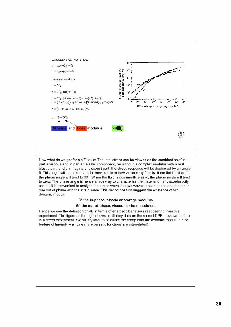
Now what do we get for a VE liquid: The total stress can be viewed as the combination of inpart a viscous and in part an elastic component, resulting in a complex modulus with a realelastic part, and an imaginary (viscous) part The stress response will be dephased by an angleδ. This angle will be a measure for how elastic or how viscous my fluid is. If the fluid is viscousthe phase angle will tend to 90°. When the fluid is dominantly elastic, the phase angle will tendto zero. The phase angle is hence a nice way to characterize the material on a “viscoelasticityscale”. It is convenient to analyze the stress wave into two waves, one in phase and the otherone out of phase with the strain wave. This decomposition suggest the existence of twodynamic moduli:

G’ the in-phase, elastic or storage modulusG” the out-of-phase, viscous or loss modulus.

Hence we see the definition of VE in terms of energetic behaviour reappearing from thisexperiment. The figure on the right shows oscillatory data on the same LDPE as shown beforein a creep experiment. We will try later to calculate the creep from the dynamic moduli (a nicefeature of linearity – all Linear viscoelastic functions are interrelated)

31

[ ]

=

=

!+!=

=

"

)"(

)cos(")sin('

MATERIALNewtonian

0

G

G

tGtG

"#

"$$#

"%# !

G” = Loss modulus ?tan =!

[ ]

=

=

!+!=

=

"

'

)'(

)cos(")sin('

MATERIAL(Hookean)Elastic

0

G

G

tGtG

G

#$

#%%$

#$

?=!

?tan =!

?=!

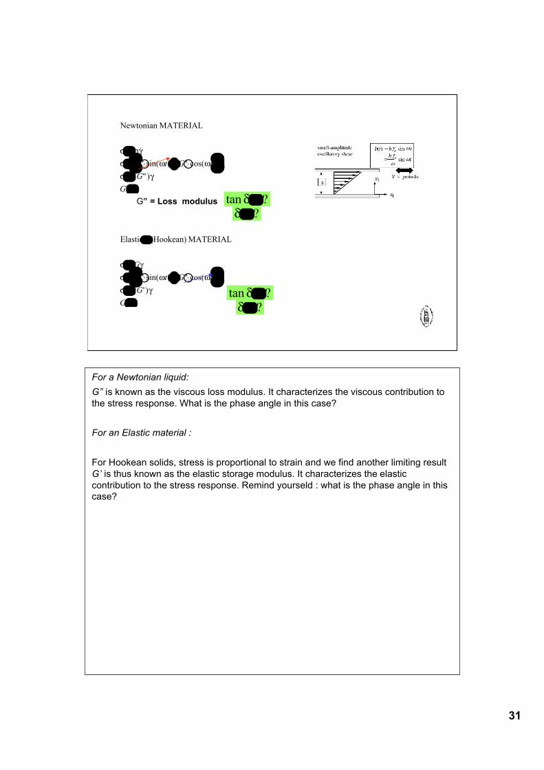
For a Newtonian liquid:G” is known as the viscous loss modulus. It characterizes the viscous contribution tothe stress response. What is the phase angle in this case?

For an Elastic material :

For Hookean solids, stress is proportional to strain and we find another limiting resultG’ is thus known as the elastic storage modulus. It characterizes the elasticcontribution to the stress response. Remind yourseld : what is the phase angle in thiscase?

32

VISCOELASTIC MATERIAL

i t

complex vis ity

i i i

G

G

G GG

! ! " #

! $ %

! $ $ "% $ $ "%

$"

$"

$" " "

= +

=

= + = &

=

=

='()

*+,

+'()

*+,

-

.//

0

122

=

3

3 3

0

2 2 1 21

exp( )

cos :

!

( ' " ) ( " ' )

'"

"'

' "/

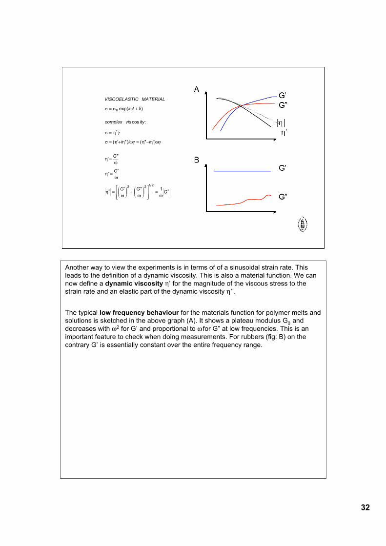
Another way to view the experiments is in terms of of a sinusoidal strain rate. Thisleads to the definition of a dynamic viscosity. This is also a material function. We cannow define a dynamic viscosity η’ for the magnitude of the viscous stress to thestrain rate and an elastic part of the dynamic viscosity η’’.

The typical low frequency behaviour for the materials function for polymer melts andsolutions is sketched in the above graph (A). It shows a plateau modulus G0 anddecreases with ω2 for G’ and proportional to ω for G” at low frequencies. This is animportant feature to check when doing measurements. For rubbers (fig: B) on thecontrary G’ is essentially constant over the entire frequency range.

33

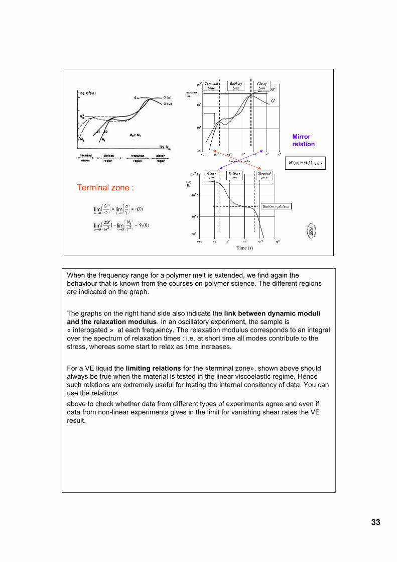
Time (s)

Terminal zone :

Mirror relation

When the frequency range for a polymer melt is extended, we find again thebehaviour that is known from the courses on polymer science. The different regionsare indicated on the graph.

The graphs on the right hand side also indicate the link between dynamic moduliand the relaxation modulus. In an oscillatory experiment, the sample is« interogated » at each frequency. The relaxation modulus corresponds to an integralover the spectrum of relaxation times : i.e. at short time all modes contribute to thestress, whereas some start to relax as time increases.

For a VE liquid the limiting relations for the «terminal zone», shown above shouldalways be true when the material is tested in the linear viscoelastic regime. Hencesuch relations are extremely useful for testing the internal consitency of data. You canuse the relationsabove to check whether data from different types of experiments agree and even ifdata from non-linear experiments gives in the limit for vanishing shear rates the VEresult.

34

Effect molecular weight onthe LV moduli of polymer

melts

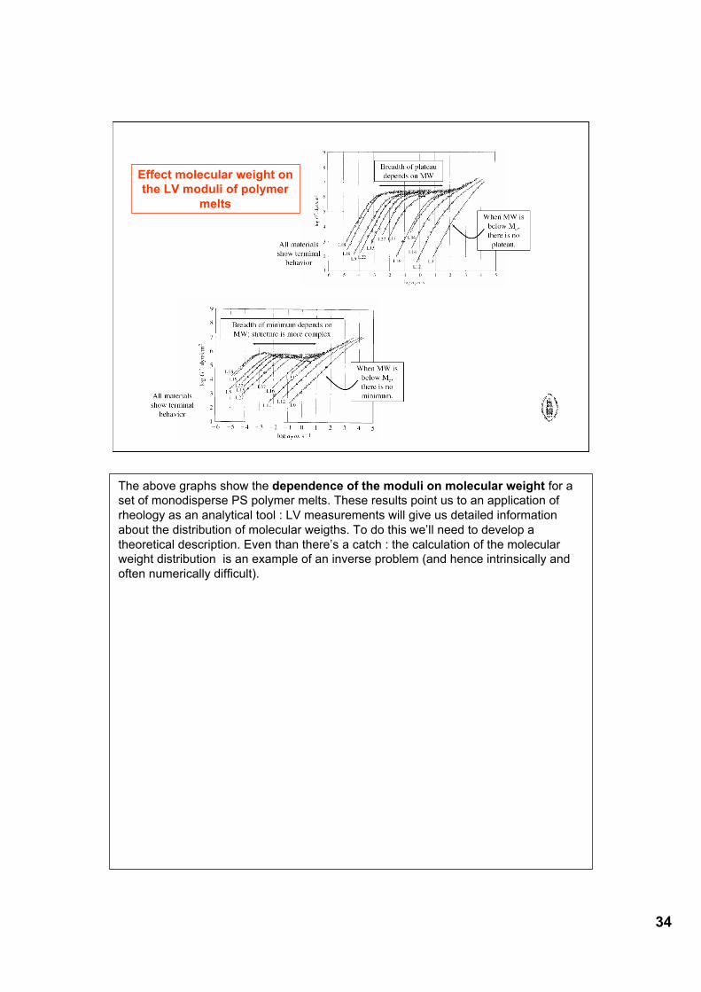
The above graphs show the dependence of the moduli on molecular weight for aset of monodisperse PS polymer melts. These results point us to an application ofrheology as an analytical tool : LV measurements will give us detailed informationabout the distribution of molecular weigths. To do this we’ll need to develop atheoretical description. Even than there’s a catch : the calculation of the molecularweight distribution is an example of an inverse problem (and hence intrinsically andoften numerically difficult).

35

Effect of volume fractionon the dynamic moduli of

dispersions

! (rad/s)

10-2 10-1 100 101 102

G' (P

a) G

"(Pa

) 10-2

10-1

100

101

102

103

104

0.421

0.426

0.437

0.452

0.455

0.471

0.482

0.502

0.515

0.534

"c

F r

d

dr

d kT N kT dc

c

c

G( )

.

'

=

!

"#

$

%&

'= (

!"#

$%&)

2

2

3

5

0 639

6

*+ ,

+

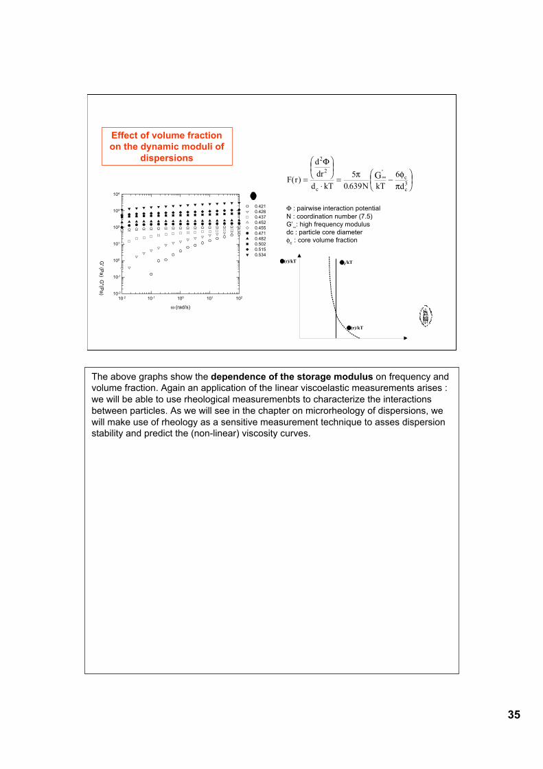
Φ : pairwise interaction potentialN : coordination number (7.5)G’∞: high frequency modulusdc : particle core diameterφc : core volume fraction

r

!(r)/kT

!(r)/kT

!d/kT

The above graphs show the dependence of the storage modulus on frequency andvolume fraction. Again an application of the linear viscoelastic measurements arises :we will be able to use rheological measuremenbts to characterize the interactionsbetween particles. As we will see in the chapter on microrheology of dispersions, wewill make use of rheology as a sensitive measurement technique to asses dispersionstability and predict the (non-linear) viscosity curves.

36

2. Differential models : The Maxwell model

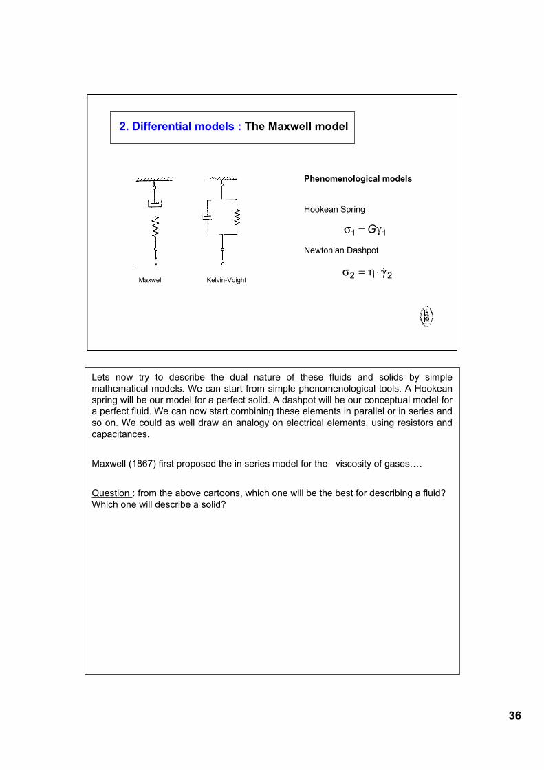
Phenomenological models

Hookean Spring

Newtonian Dashpot

Maxwell Kelvin-Voight

! "1 1=G

! " #2 2= $ !

Lets now try to describe the dual nature of these fluids and solids by simplemathematical models. We can start from simple phenomenological tools. A Hookeanspring will be our model for a perfect solid. A dashpot will be our conceptual model fora perfect fluid. We can now start combining these elements in parallel or in series andso on. We could as well draw an analogy on electrical elements, using resistors andcapacitances.

Maxwell (1867) first proposed the in series model for the viscosity of gases….

Question : from the above cartoons, which one will be the best for describing a fluid?Which one will describe a solid?

37

! ! !

" " "

! ! !

!" "

#

"#

" # !

" $" # !

= +

= =

= +

= +

+%&'

()* =

+ =

1 2

1 2

1 2

1

0

2

0

0

0

0

0

! ! !

!!

! !

! !

G

G

τ = relaxation time

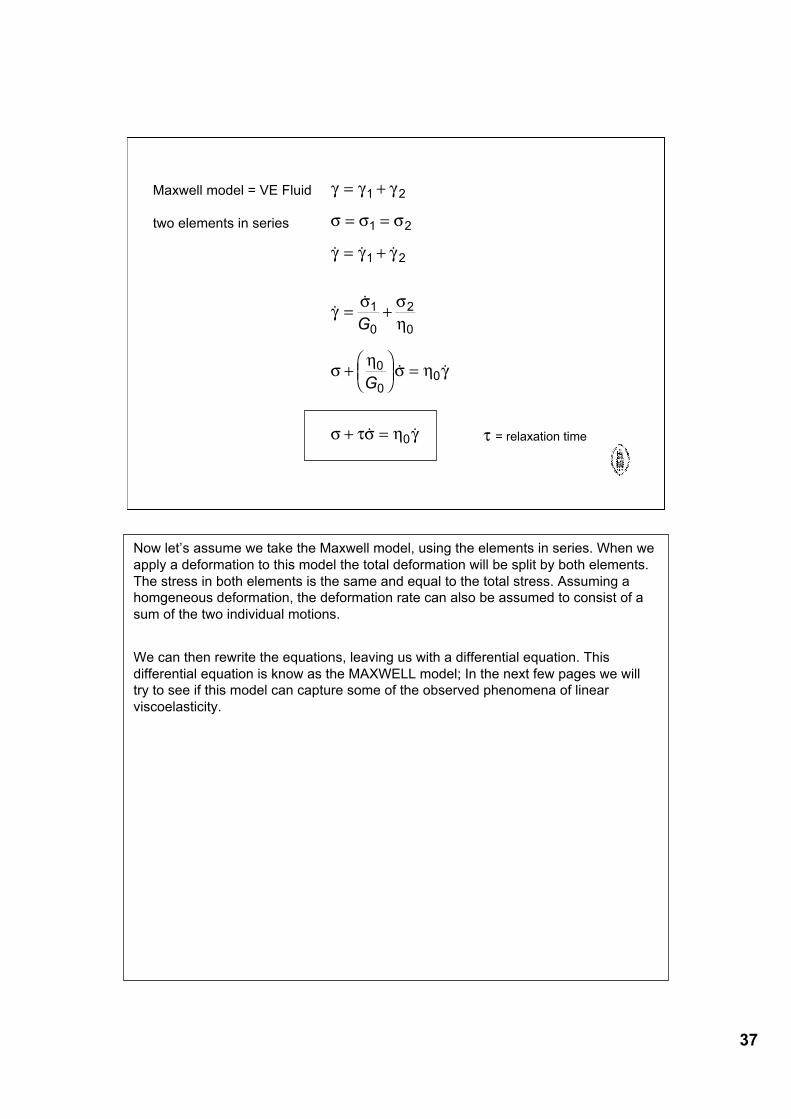
Maxwell model = VE Fluid

two elements in series

Now let’s assume we take the Maxwell model, using the elements in series. When weapply a deformation to this model the total deformation will be split by both elements.The stress in both elements is the same and equal to the total stress. Assuming ahomgeneous deformation, the deformation rate can also be assumed to consist of asum of the two individual motions.

We can then rewrite the equations, leaving us with a differential equation. Thisdifferential equation is know as the MAXWELL model; In the next few pages we willtry to see if this model can capture some of the observed phenomena of linearviscoelasticity.

38

! [rad/s]

0.01 0.1 1 10

G(t)

0

2

4

6

8

10

12

"

G0

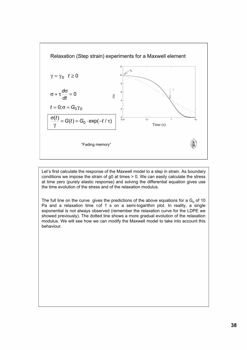
Relaxation (Step strain) experiments for a Maxwell element

! !

" #"

" !

"

!#

= $

+ =

= =

= = % &

0

0 0

0

0

0

0

t

d

dt

t G

tG t G t

;

( )( ) exp( / )

“Fading memory”

Time (s)

Let’s first calculate the response of the Maxwell model to a step in strain. As boundaryconditions we impose the strain of g0 at times > 0. We can easily calculate the stressat time zero (purely elastic response) and solving the differential equation gives usethe time evolution of the stress and of the relaxation modulus.

The full line on the curve gives the predictions of the above equations for a G0 of 10Pa and a relaxation time τ of 1 s on a semi-logarithm plot. In reality, a singleexponential is not always observed (remember the relaxation curve for the LDPE weshowed previously). The dotted line shows a more gradual evolution of the relaxationmodulus. We will see how we can modify the Maxwell model to take into account thisbehaviour.

39

Dynamic moduli

w [rad/s]

0.01 0.1 1 10 100

Mo

du

li [Pa

]

0.001

0.01

0.1

1

10

G'

G"

G0

!

GG

GG

'( )

"( )

!! "

! "

!!"

! "

=

+

=

+

02 2

2 2

02 2

1

1

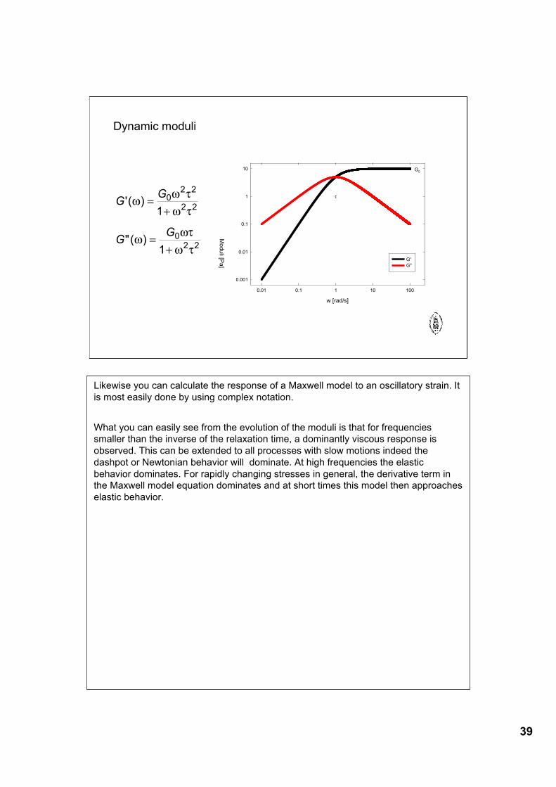
Likewise you can calculate the response of a Maxwell model to an oscillatory strain. Itis most easily done by using complex notation.

What you can easily see from the evolution of the moduli is that for frequenciessmaller than the inverse of the relaxation time, a dominantly viscous response isobserved. This can be extended to all processes with slow motions indeed thedashpot or Newtonian behavior will dominate. At high frequencies the elasticbehavior dominates. For rapidly changing stresses in general, the derivative term inthe Maxwell model equation dominates and at short times this model then approacheselastic behavior.

40

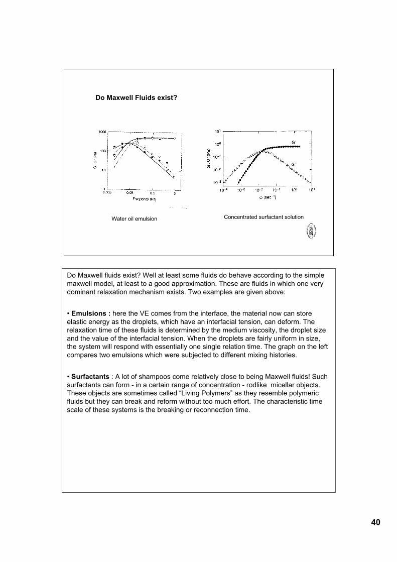
Do Maxwell Fluids exist?

Water oil emulsion Concentrated surfactant solution

Do Maxwell fluids exist? Well at least some fluids do behave according to the simplemaxwell model, at least to a good approximation. These are fluids in which one verydominant relaxation mechanism exists. Two examples are given above:

• Emulsions : here the VE comes from the interface, the material now can storeelastic energy as the droplets, which have an interfacial tension, can deform. Therelaxation time of these fluids is determined by the medium viscosity, the droplet sizeand the value of the interfacial tension. When the droplets are fairly uniform in size,the system will respond with essentially one single relation time. The graph on the leftcompares two emulsions which were subjected to different mixing histories.

• Surfactants : A lot of shampoos come relatively close to being Maxwell fluids! Suchsurfactants can form - in a certain range of concentration - rodlike micellar objects.These objects are sometimes called “Living Polymers” as they resemble polymericfluids but they can break and reform without too much effort. The characteristic timescale of these systems is the breaking or reconnection time.

41

Can we describe polymer melts?

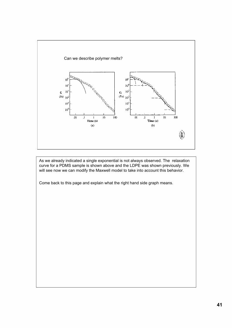
As we already indicated a single exponential is not always observed. The relaxationcurve for a PDMS sample is shown above and the LDPE was shown previously. Wewill see now we can modify the Maxwell model to take into account this behavior.

Come back to this page and explain what the right hand side graph means.

42

An obvious way to generalize the Maxwell model is to allow for multiple relaxationtimes. This can be done by considering multiple dashpot-spring combinations inparallel. In this manner, several relaxation times are available to fit our experimentaldata.

The relaxation data of the PDMS on the previous page could be described byselecting a set of relaxation times equidistantly spaced on a logarithmic axis anddetermining the Gk’s for the different modes by a linear regression analysis. (τk = 0.01,0.1, 1, 10, 100 s, Gk=2*105, 105, 104,102,10) .

Some molecular theories, like the Rouse theory for polymer dynamics (see later)suggest an infinite series of relaxation times where only two fit parameters remain.

Generalized Maxwell model

! !

! " ! # $

"

TOT ii

i i i i

ii

iG t G t

= %

+ =

= &%

! !

( ) exp( / )0

Jeffreys model

! " ! # $ "$

+ = +%&'

()*1 2

! !!d

dt

G G

k

k

k

k

k

k

O

=

=

!0

2

"

"

""

43

3. General viscoelastic Integral model

ds

sdGfunctionmemorysM

ttsdsssMt

ttdGtGtGt

dtdt

dttGt

tdttGt

tttGt

t

t

t

)()(

')()()(

)'()'()()()()()(

''

)'()(

)'()'()(

)'()'()(

==

!==

!!!""!=

!=

!=

!=

#

#

#

#

$

"!

"!

"!

%&

%%%&

%&

%&

%'&

0

fluid

Reference state @ t=0

! (t) = M(s)" (s)ds

0

#

$

s = t ! t '

M(s) =dg(s)

ds is the memory function

An arbitrary evolution of deformation in time can be approximated by a series ofstepwise changes Δγ . If we assume that the stress a time t resulting from the givenmotion equals the sum of the partial stresses at time t from the individual strains Δγat time (t’) (this is what is called the linearity or Boltzman principle), the total stresscan be calculated as indicated above.

When the steps are taken to be infinitesimally small, the summation becomes anintegration. Note that in rheology it is customary to use the configuration at time t asthe reference. The equation can then be transformed by an integration by parts.

Noting that G(∞)=0 for fluids and γ is finite at time t’ = ∞ that γ(t)=0 is a reference forthe deformation.

44

What is the relaxation function?For a simple Maxwell model we used a single exponential

G t G t

G t G t

G t Ftd

G t Ht d

i i

( ) exp( / )

( ) exp( / )

( ) ( )exp

( ) ( )exp

= !

= !"

=!#

$%&'()

=!#

$%&'()

*

*

0

0

0

+

+

++

+

++

++

For a generalized Maxwell fluid this becomes

We can replace the discrete relaxation times by a continuous spectrum

Often one use a logaritmic scale : the relaxation spectrum is defined as follows

Powerful way to characterizematerials - albeit in the Linear region

The use of G(s) does not lead directly to a specific equation for the stress relaxationfunction. Specific expressions can be developed. By using a simplest expression is asingle exponential decrease. In this manner we obtain the integral formulation of theMaxwell model. The integral form of the generalized Maxwell model can be easilyobtained by using the relaxation spectrum as defined above.

By using a relaxation spectrum, any arbitrary relaxation function can be fittedaccurately in a unique manner. This provides a very powerful tool to characterize therheological behavior of polymers. The relaxation spectrum allows one to obtain a“dynamic fingerprint” of the behavior of polymers. For linear polymers, the relaxationspectrum can be linked to the molecular weight and the molecular weight distribution.

45

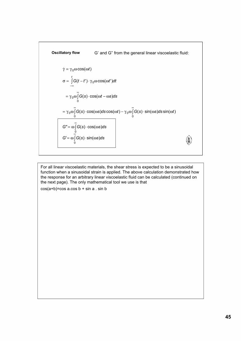
G’ and G” from the general linear viscoelastic fluid:Oscillatory flow

! cos( )

( ') cos( ')

( ) cos( )

( ) cos( ) cos( ) ( ) sin( ) sin( )

" ( ) cos( )

' ( ) sin( )

! ! " "

# ! " "

! " " "

! " " " ! " " "

" "

" "

=

= $ %

= % $

= % $ %

= %

= %

$&

&

& &

&

&

'

'

' '

'

'

0

0

00

00

00

0

0

t

G t t t dt

G s t s ds

G s s ds t G s s ds t

G G s s ds

G G s s ds

t

For all linear viscoelastic materials, the shear stress is expected to be a sinusoidalfunction when a sinusoidal strain is applied. The above calculation demonstrated howthe response for an arbitrary linear viscoelastic fluid can be calculated (continued onthe next page). The only mathematical tool we use is thatcos(a+b)=cos a.cos b + sin a . sin b

46

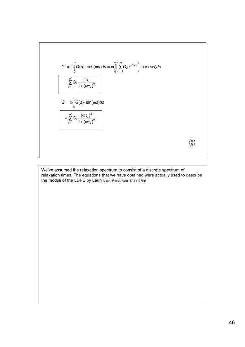
G G s s ds G e s ds

G

G G s s ds

G

ii s

i

N

ii

ii

N

ii

ii

N

" ( ) cos( ) cos( )

( )

' ( ) sin( )

( )

( )

= ! ="#$

%&'!

=

+

= !

=

+

()

=

(

=

(

=

* +*

+

*

+

, , , - ,

,-,-

, ,

,-,-

0 10

21

0

2

21

1

1

We’ve assumed the relaxation spectrum to consist of a discrete spectrum ofrelaxation times. The equations that we have obtained were actually used to describethe moduli of the LDPE by Laun [Laun, Rheol. Acta, 17,1 (1978)]

47

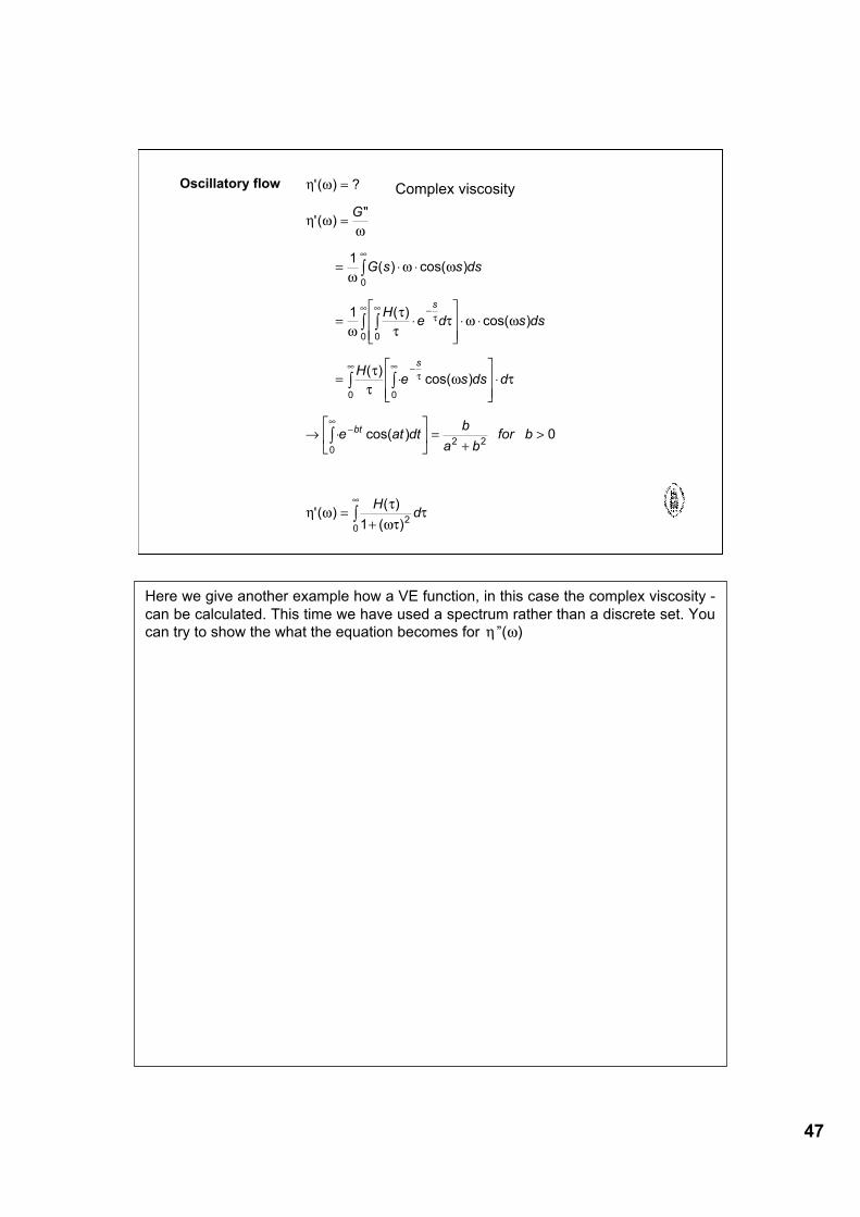
Complex viscosity Oscillatory flow ! "

! ""

"" "

"##

# " "

##

" #

! "#

"##

#

#

'( ) ?

'( )"

( ) cos( )

( )cos( )

( )cos( )

cos( )

'( )( )

( )

=

=

= $ $

= $%

&''

(

)**$ $

= $%

&''

(

)**$

+ $%

&'

(

)* =

+

>

=

+

,

-,,

-,,

-,

,

.

..

..

.

.

G

G s s ds

He d s ds

He s ds d

e at dtb

a bfor b

Hd

s

s

bt

1

1

0

1

0

00

00

02 2

20

Here we give another example how a VE function, in this case the complex viscosity -can be calculated. This time we have used a spectrum rather than a discrete set. Youcan try to show the what the equation becomes for η ”(ω)

48

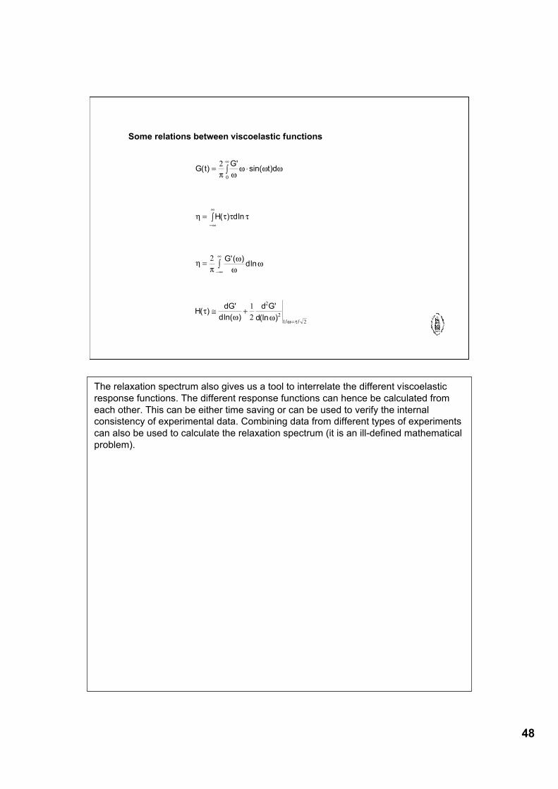
Some relations between viscoelastic functions

G tG

t d

H d

Gd

HdG

d

d G

d

( )'

sin( )

( ) ln

'( )ln

( )'

ln( )

'

(ln )/ /

= !

=

=

" +

#

$#

#

$#

#

=

%

%

%

2

2

1

2

0

2

2

1 2

& '' ' '

( ) ) )

(&

''

'

)' '

' )

The relaxation spectrum also gives us a tool to interrelate the different viscoelasticresponse functions. The different response functions can hence be calculated fromeach other. This can be either time saving or can be used to verify the internalconsistency of experimental data. Combining data from different types of experimentscan also be used to calculate the relaxation spectrum (it is an ill-defined mathematicalproblem).

49

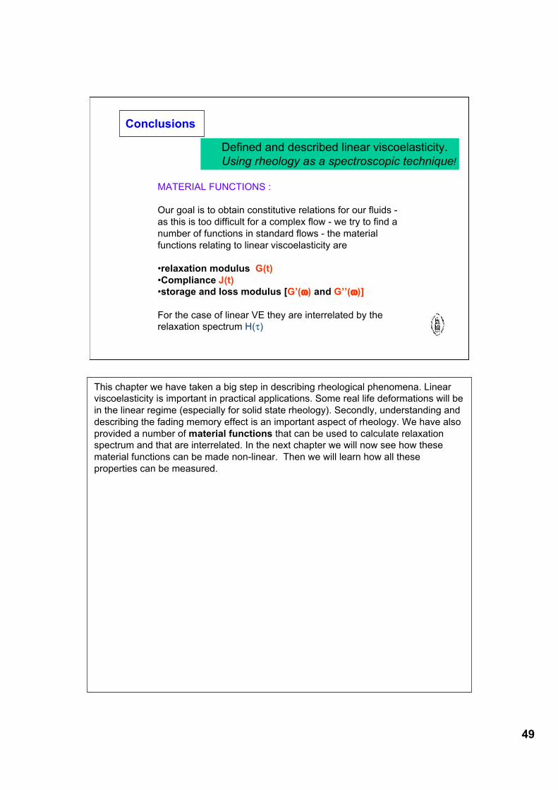
MATERIAL FUNCTIONS :

Our goal is to obtain constitutive relations for our fluids -as this is too difficult for a complex flow - we try to find anumber of functions in standard flows - the materialfunctions relating to linear viscoelasticity are

•relaxation modulus G(t)•Compliance J(t)•storage and loss modulus [G’(ω) and G’’(ω)]

For the case of linear VE they are interrelated by therelaxation spectrum H(τ)

Conclusions

Defined and described linear viscoelasticity.Using rheology as a spectroscopic technique!

This chapter we have taken a big step in describing rheological phenomena. Linearviscoelasticity is important in practical applications. Some real life deformations will bein the linear regime (especially for solid state rheology). Secondly, understanding anddescribing the fading memory effect is an important aspect of rheology. We have alsoprovided a number of material functions that can be used to calculate relaxationspectrum and that are interrelated. In the next chapter we will now see how thesematerial functions can be made non-linear. Then we will learn how all theseproperties can be measured.

50

Applied Rheology

Generalized NewtonianFluids

Although Newton’s law is of much practical use, at the beginning of this centuryresearchers started to realize that not all fluids obey this simple linear relation. Manycolloidal suspensions and polymer solutions show a decrease of the viscosity as theshear rate is increased.

In the following, we will try to extend Newton’s law in the most simple fashion, bymaking the stress depend on the rate of deformation (or better : on an invariant of therate of deformation tensor). But as we are talking about viscosities and rate ofdeformations, maybe it is useful to start of with indicating a few orders of magnitudeswhich are likely to be encountered

51

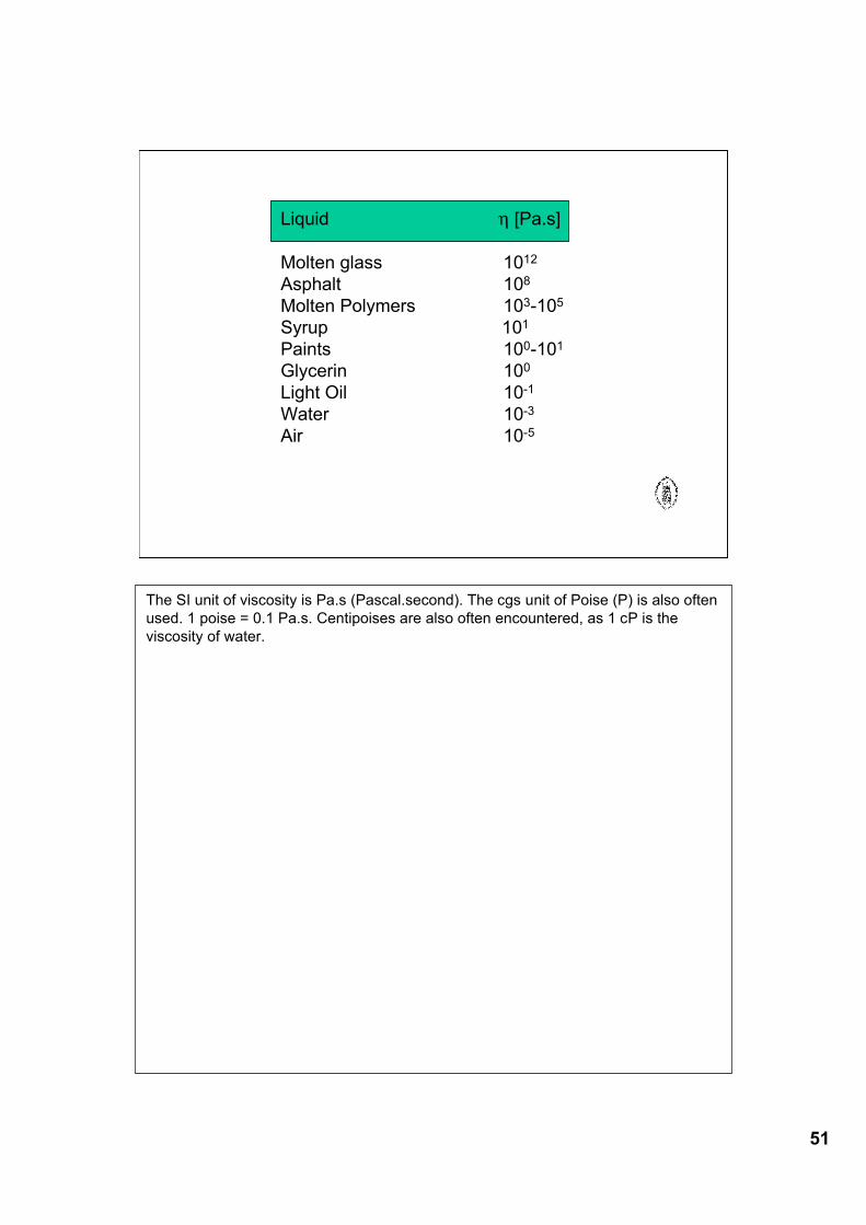
Liquid η [Pa.s]

Molten glass 1012

Asphalt 108

Molten Polymers 103-105

Syrup 101

Paints 100-101

Glycerin 100

Light Oil 10-1

Water 10-3

Air 10-5

The SI unit of viscosity is Pa.s (Pascal.second). The cgs unit of Poise (P) is also oftenused. 1 poise = 0.1 Pa.s. Centipoises are also often encountered, as 1 cP is theviscosity of water.

52

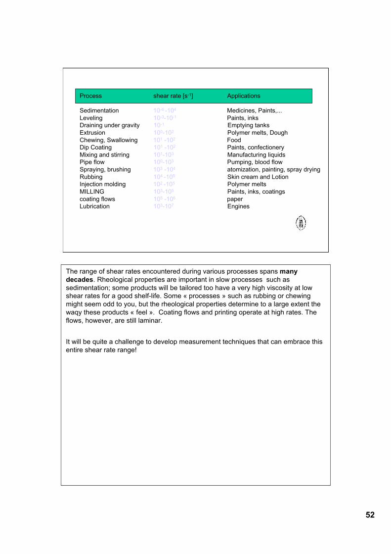
Process shear rate [s-1] Applications

Sedimentation 10-6 -104 Medicines, Paints,...Leveling 10-3-10-1 Paints, inksDraining under gravity 10-1 Emptying tanksExtrusion 100-102 Polymer melts, DoughChewing, Swallowing 101 -102 FoodDip Coating 101 -102 Paints, confectioneryMixing and stirring 101-103 Manufacturing liquidsPipe flow 100-103 Pumping, blood flowSpraying, brushing 103 -104 atomization, painting, spray dryingRubbing 104 -105 Skin cream and LotionInjection molding 102 -105 Polymer meltsMILLING 103-105 Paints, inks, coatingscoating flows 105 -106 paperLubrication 103-107 Engines

The range of shear rates encountered during various processes spans manydecades. Rheological properties are important in slow processes such assedimentation; some products will be tailored too have a very high viscosity at lowshear rates for a good shelf-life. Some « processes » such as rubbing or chewingmight seem odd to you, but the rheological properties determine to a large extent thewaqy these products « feel ». Coating flows and printing operate at high rates. Theflows, however, are still laminar.

It will be quite a challenge to develop measurement techniques that can embrace thisentire shear rate range!

53

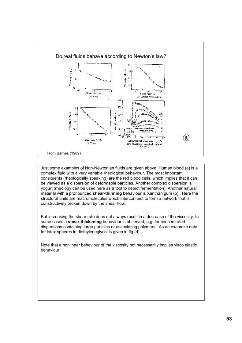
Do real fluids behave according to Newton’s law?

From Barnes (1989)

Just some examples of Non-Newtonian fluids are given above. Human blood (a) is acomplex fluid with a very variable rheological behaviour. The most importantconsituents (rheologically speaking) are the red blood cells, which implies that it canbe viewed as a dispersion of deformable particles. Another complex dispersion isyogurt (rheology can be used here as a tool to detect fermentation). Another naturalmaterial with a pronounced shear-thinning behaviour is Xanthan gum (b) . Here thestructural units are macromolecules which interconnect to form a network that isconstructively broken down by the shear flow.

But increasing the shear rate does not always result in a decrease of the viscosity. Insome cases a shear-thickening behaviour is observed, e.g. for concentrateddispersions containing large particles or associating polymers. As an examoke datafor latex spheres in diethyleneglycol is given in fig (d).

Note that a nonlinear behaviour of the viscosity not necessarilly implies visco elasticbehaviour.

54

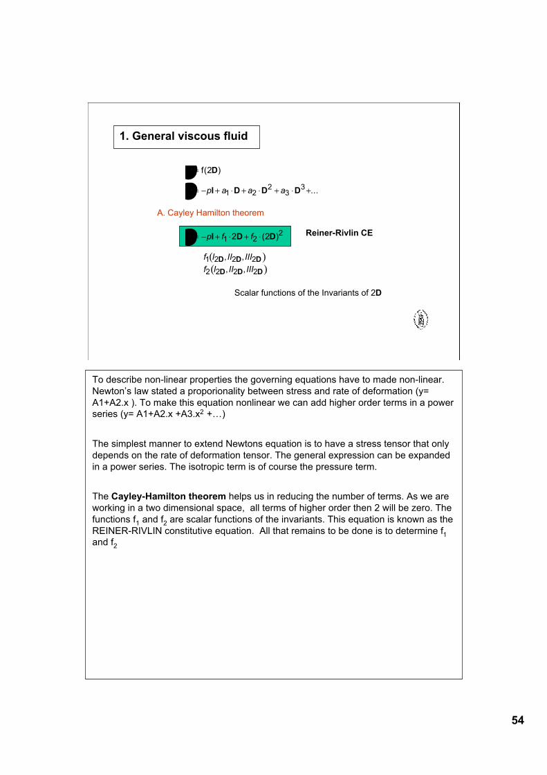
1. General viscous fluid

( )

( )

!

!

!

=

= " + # + # + # +

= " + # + #

f( )

...

( )

, ,

, ,

2

2 2

1 22

33

1 22

1 2 2 2

2 2 2 2

D

I D D D

I D D

D D D

D D D

p a a a

p f f

f I II III

f I II III

Reiner-Rivlin CE

A. Cayley Hamilton theorem

Scalar functions of the Invariants of 2D

To describe non-linear properties the governing equations have to made non-linear.Newton’s law stated a proporionality between stress and rate of deformation (y=A1+A2.x ). To make this equation nonlinear we can add higher order terms in a powerseries (y= A1+A2.x +A3.x2 +…)

The simplest manner to extend Newtons equation is to have a stress tensor that onlydepends on the rate of deformation tensor. The general expression can be expandedin a power series. The isotropic term is of course the pressure term.

The Cayley-Hamilton theorem helps us in reducing the number of terms. As we areworking in a two dimensional space, all terms of higher order then 2 will be zero. Thefunctions f1 and f2 are scalar functions of the invariants. This equation is known as theREINER-RIVLIN constitutive equation. All that remains to be done is to determine f1and f2

55

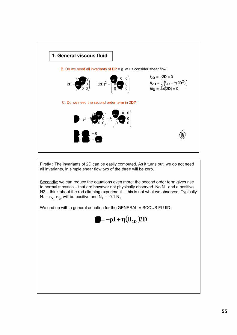
1. General viscous fluid

( )I

II I tr

III

2

2 22

2 01

22

2 0

D

D D

D

D

D

D

= =

= !

= =

tr

( )

det( )

B. Do we need all invariants of D? e.g. et us consider shear flow

C. Do we need the second order term in 2D?

2 2

0

02

2

2D D=

!

"##

$

%&&

=

!

"

####

$

%

&&&&

0 00 0

0 0 0

0

00 0 0

!

! ( )

!

!

''

'

'

!"

"

"

"

! !

! ! "

= # +

$

%&&

'

())+

$

%

&&&&

'

(

))))

# =

# =

p f f

f

xx yy

yy zz

I 1 2

2

2

22

0

0

0

0 0

0 0

0 0 0

0

0

0 0 0

!

!

!

!

!

Firstly : The invariants of 2D can be easily computed. As it turns out, we do not needall invariants, in simple shear flow two of the three will be zero.

Secondly: we can reduce the equations even more: the second order term gives riseto normal stresses – that are however not physically observed. No N1 and a positiveN2 – think about the rod climbing experiment – this is not what we observed. TypicallyN1 = σxx-σyy will be positive and N2 = -0.1 N1

We end up with a general equation for the GENERAL VISCOUS FLUID:

( ) DID2IIp 2!+"=#

56

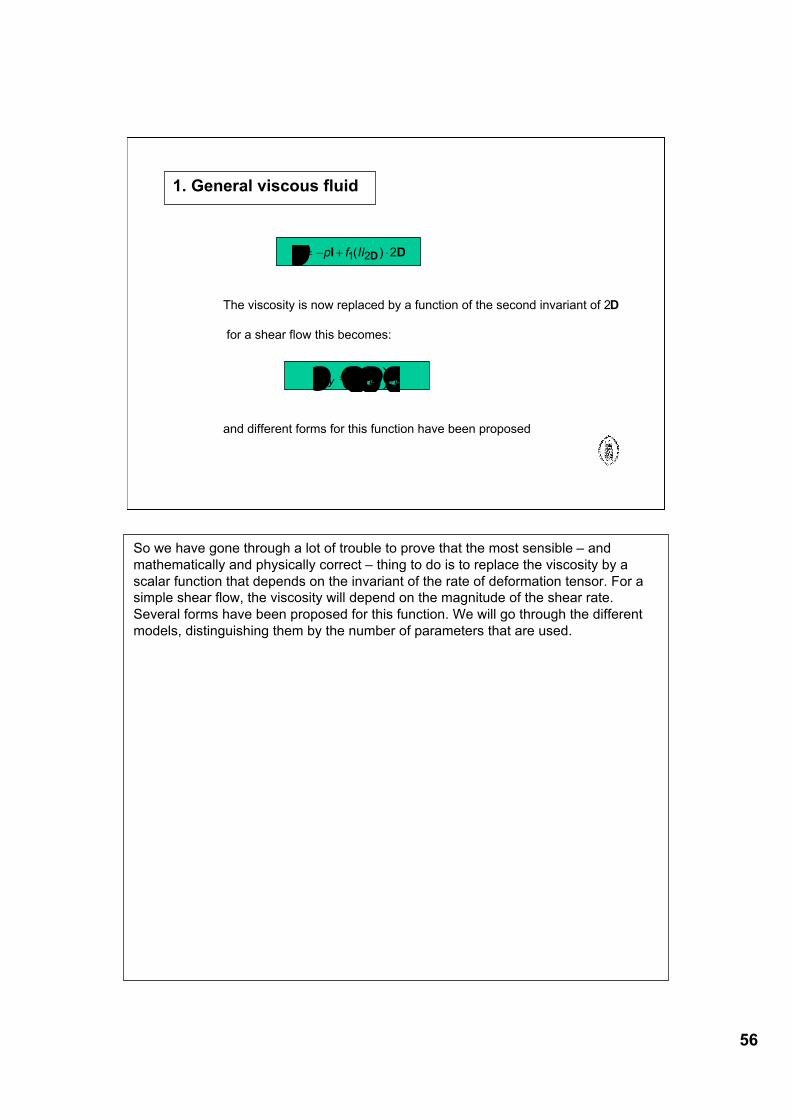
1. General viscous fluid

! = " + #p f III DD1 2 2( )

The viscosity is now replaced by a function of the second invariant of 2D

for a shear flow this becomes:

and different forms for this function have been proposed

( )! " # #xy = $12! !

So we have gone through a lot of trouble to prove that the most sensible – andmathematically and physically correct – thing to do is to replace the viscosity by ascalar function that depends on the invariant of the rate of deformation tensor. For asimple shear flow, the viscosity will depend on the magnitude of the shear rate.Several forms have been proposed for this function. We will go through the differentmodels, distinguishing them by the number of parameters that are used.

57

! (Pa)

10-3 10-2 10-1 100 101 102 103 104 105

"

(Pa

s)

10-3

10-2

10-1

100

101

102# = 0.50

0.47

0.43

0.34

0.280.18

H2O

Styrene-ethylacrylate in H2O

2a = 250 nm

Viscosity curves :

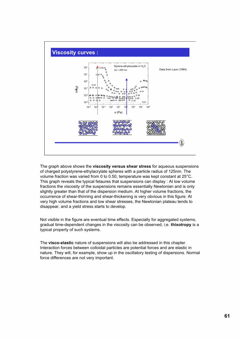
Data from Laun (1984)

The graph above shows the viscosity versus shear stress for aqueous suspensionsof charged polystyrene-ethylacrylate spheres with a particle radius of 125nm. Thevolume fraction was varied from 0 to 0.50, temperature was kept constant at 25°C.This graph reveals the typical fetaures that suspensions can display : At low volumefractions the viscosity of the suspensions remains essentially Newtonian and is onlyslightly greater than that of the dispersion medium. At higher volume fractions, theoccurrence of shear-thinning and shear-thickening is very obvious in this figure. Atvery high volume fractions and low shear stresses, the Newtonian plateau tends todisappear, and a yield stress starts to develop.

Not visible in the figure are eventual time effects. Especially for aggregated systems,gradual time-dependent changes in the viscosity can be observed, i;e. thixotropy is atypical property of such systems.

The visco-elastic nature of suspensions will also be addressed in this chapter.Interaction forces between colloidal particles are potential forces and are elastic innature. They will, for example, show up in the oscillatory testing of dispersions. Normalforce differences are not very important.

58

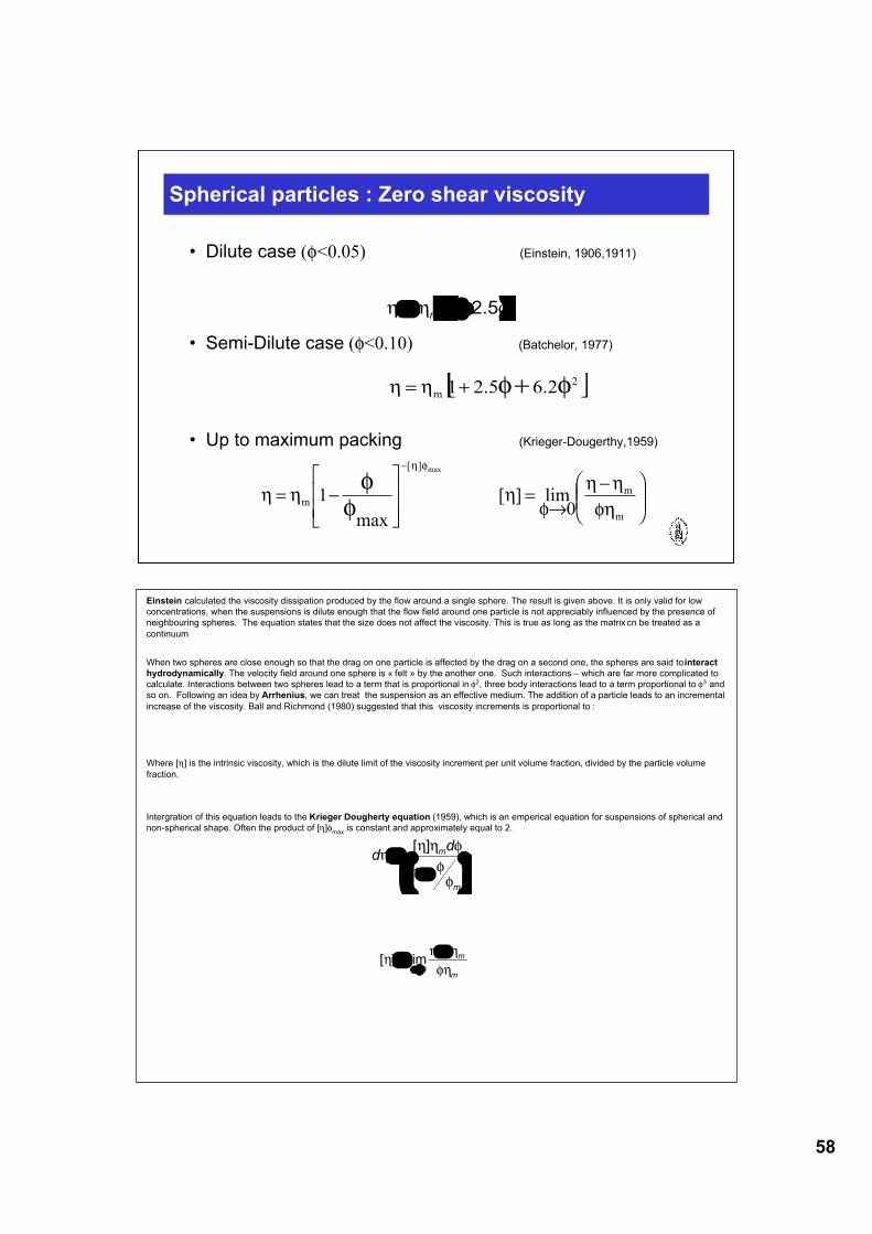
Spherical particles : Zero shear viscosity

• Dilute case (φ<0.05) (Einstein, 1906,1911)

[ ]!"" 2.51+=m

• Semi-Dilute case (φ<0.10) (Batchelor, 1977)

[ ]2m

6.22.51 !+!+"="

• Up to maximum packing (Krieger-Dougerthy,1959)

!!"

#$$%

&'(()(

*'=(

++,

-

.

./

0)(=(

'()

''

m

m

][

m0

lim][

max

1

max

Einstein calculated the viscosity dissipation produced by the flow around a single sphere. The result is given above. It is only valid for lowconcentrations, when the suspensions is dilute enough that the flow field around one particle is not appreciably influenced by the presence ofneighbouring spheres. The equation states that the size does not affect the viscosity. This is true as long as the matrix cn be treated as acontinuum

When two spheres are close enough so that the drag on one particle is affected by the drag on a second one, the spheres are said to interacthydrodynamically. The velocity field around one sphere is « felt » by the another one. Such interactions – which are far more complicated tocalculate. Interactions between two spheres lead to a term that is proportional in φ2, three body interactions lead to a term proportional to φ3 andso on. Following an idea by Arrhenius, we can treat the suspension as an effective medium. The addition of a particle leads to an incrementalincrease of the viscosity. Ball and Richmond (1980) suggested that this viscosity increments is proportional to :

Where [η] is the intrinsic viscosity, which is the dilute limit of the viscosity increment per unit volume fraction, divided by the particle volumefraction.

Intergration of this equation leads to the Krieger Dougherty equation (1959), which is an emperical equation for suspensions of spherical andnon-spherical shape. Often the product of [η]φmax is constant and approximately equal to 2.

!"#$

%& '

=

m

md

d

((

()))

1

][

m

m

!"

"""

!

#=

$0lim][

59

!

0.0 0.1 0.2 0.3 0.4 0.5 0.6 0.7

"/"

s

1

10

100

1000

Einstein

Batchelor

Krieger-Dougherty

Spherical particles : Zero shear viscosity

Φmax

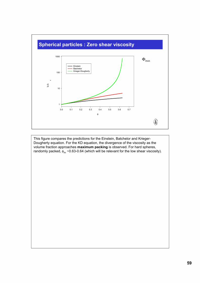
This figure compares the predictions for the Einstein, Batchelor and Krieger-Dougherty equation. For the KD equation, the divergence of the viscosity as thevolume fraction approaches maximum packing is observed. For hard spheres,randomly packed, φm ~0.63-0.64 (which will be relevant for the low shear viscosity).

60

Spherical particles : Zero shear viscosity

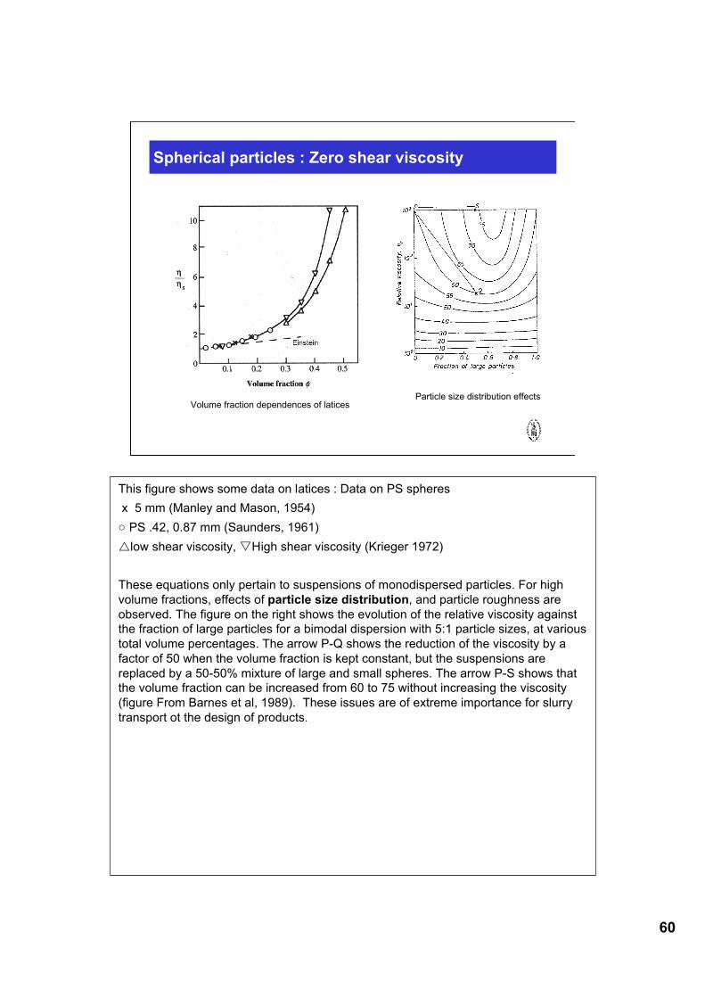
Volume fraction dependences of laticesParticle size distribution effects

This figure shows some data on latices : Data on PS spheres x 5 mm (Manley and Mason, 1954)○ PS .42, 0.87 mm (Saunders, 1961)low shear viscosity, High shear viscosity (Krieger 1972)

These equations only pertain to suspensions of monodispersed particles. For highvolume fractions, effects of particle size distribution, and particle roughness areobserved. The figure on the right shows the evolution of the relative viscosity againstthe fraction of large particles for a bimodal dispersion with 5:1 particle sizes, at varioustotal volume percentages. The arrow P-Q shows the reduction of the viscosity by afactor of 50 when the volume fraction is kept constant, but the suspensions arereplaced by a 50-50% mixture of large and small spheres. The arrow P-S shows thatthe volume fraction can be increased from 60 to 75 without increasing the viscosity(figure From Barnes et al, 1989). These issues are of extreme importance for slurrytransport ot the design of products.

61

! (Pa)

10-3 10-2 10-1 100 101 102 103 104 105

"

(Pa

s)

10-3

10-2

10-1

100

101

102# = 0.50

0.47

0.43

0.34

0.280.18

H2O

Styrene-ethylacrylate in H2O

2a = 250 nm

Viscosity curves :

Data from Laun (1984)

The graph above shows the viscosity versus shear stress for aqueous suspensionsof charged polystyrene-ethylacrylate spheres with a particle radius of 125nm. Thevolume fraction was varied from 0 to 0.50, temperature was kept constant at 25°C.This graph reveals the typical fetaures that suspensions can display : At low volumefractions the viscosity of the suspensions remains essentially Newtonian and is onlyslightly greater than that of the dispersion medium. At higher volume fractions, theoccurrence of shear-thinning and shear-thickening is very obvious in this figure. Atvery high volume fractions and low shear stresses, the Newtonian plateau tends todisappear, and a yield stress starts to develop.

Not visible in the figure are eventual time effects. Especially for aggregated systems,gradual time-dependent changes in the viscosity can be observed, i;e. thixotropy is atypical property of such systems.

The visco-elastic nature of suspensions will also be addressed in this chapter.Interaction forces between colloidal particles are potential forces and are elastic innature. They will, for example, show up in the oscillatory testing of dispersions. Normalforce differences are not very important.

62

1. Large particles: Hydrodynamic Forces

Stokesian dynamics simulations (J. Brady and coworkers)

So far, we have only discussed the effects of particle volume fraction on the increase of the low shear viscosity. The viscosity of suspensions is,however, strongly dependent on shear rate. The shear rate dependence of the viscosity occurs because shear flow will be able to distort theequilibrium microstructure. The interparticle spacings will be altered, changing the magnitudes of both the hydrodynamic and the interparticleforces. This will lead to shear thinning and shear thickening.

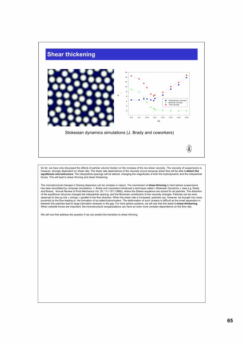
The microstructural changes in flowing dispersion can be complex in nature. The mechanism of shear-thinning in hard sphere suspensionshas been elucidated by computer simulations. J. Brady and coworkers introduced a technique called « Stokesian Dynamics » (see e.g. Bradyand Bossis, Annual Review of Fluid Mechanics Vol. 20: 111-157 (1988)), where the Stokes equations are solved for all particles. The distortionof the equilibrium structure changes the interparticle spacing, and the Brownian contribution to the viscosity changes. Particles can be evenobserved to line-up into « strings » parallel to the flow direction. When the shear rate is increased, particles can, however, be brought into closeproximity by the flow leading to the formation of so-called hydroclusters. The deformation of such clusters is difficult as the small separation inbetween the particles lead to large lubrication stresses in the gap. For hard sphere systems, we will see that this leads to shear-thickening.When colloidal forces are important, the microstructural reorganizations can have an even more complex dependence on the flow rate.

We will now first address the question if we can predict the transition to shear thinning.

63

Scaling for Brownian hard spheres

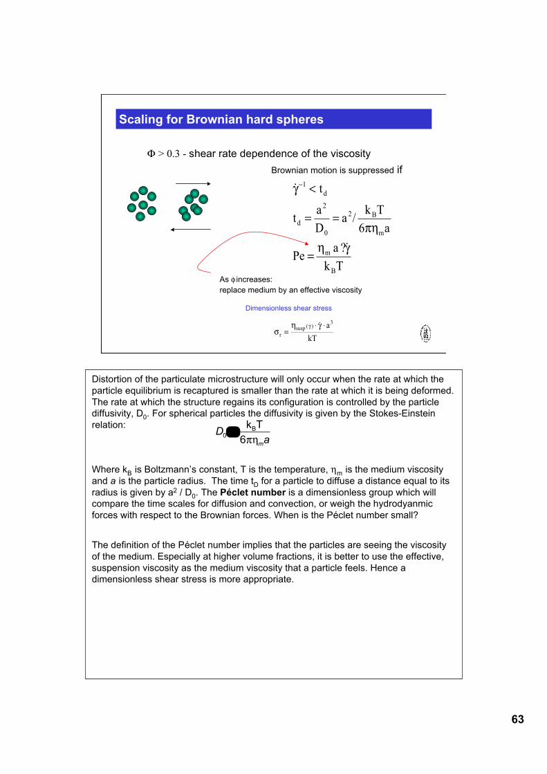
Φ > 0.3 - shear rate dependence of the viscosityBrownian motion is suppressed if

Tk

?aPe

a6

Tk/a

D

at

t

B

m

m

B2

0

2

d

d

1

!"=

#"==

<!$

!

!

As φ increases:replace medium by an effective viscosity

Dimensionless shear stress

!" ##

r

susp a

kT=

$ $( ! ) !3

Distortion of the particulate microstructure will only occur when the rate at which theparticle equilibrium is recaptured is smaller than the rate at which it is being deformed.The rate at which the structure regains its configuration is controlled by the particlediffusivity, D0. For spherical particles the diffusivity is given by the Stokes-Einsteinrelation:

Where kB is Boltzmann’s constant, T is the temperature, ηm is the medium viscosityand a is the particle radius. The time tD for a particle to diffuse a distance equal to itsradius is given by a2 / D0. The Péclet number is a dimensionless group which willcompare the time scales for diffusion and convection, or weigh the hydrodyanmicforces with respect to the Brownian forces. When is the Péclet number small?

The definition of the Péclet number implies that the particles are seeing the viscosityof the medium. Especially at higher volume fractions, it is better to use the effective,suspension viscosity as the medium viscosity that a particle feels. Hence adimensionless shear stress is more appropriate.

aD

m!"6

TkB

0=

64

!

0.0 0.2 0.4 0.6 0.8 1.0

"

r

1

10

100

1000

10000

"r0

"r#

[ ]

!"

#$%

&+

'+=

!"

#$%

&+

'+=

!"

#$%

&'=

=

((

((

'

)*+,

-.

m

r

rr

rr

r

rr

rr

r

r

b

b

f

)(1

1

1

,

0

0

max

max

/00

00

/00

00

11

0

/1010

Φmax!

!"#$

%&

!"#$

%&

=

==

Pe

RePe

,

,,,,

'(

)'(((

f

tf

r

rrmed

susp

65

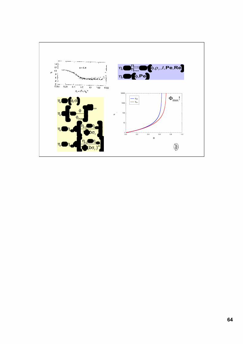
Shear thickening

Stokesian dynamics simulations (J. Brady and coworkers)

Pe

1e-2 1e-1 1e+0 1e+1 1e+2 1e+3 1e+4 1e+5

!

r

0

2

4

6

8

10

12

14

16

Hydrodynamic viscosity

Brownian viscosity

Total viscosity

So far, we have only discussed the effects of particle volume fraction on the increase of the low shear viscosity. The viscosity of suspensions is,however, strongly dependent on shear rate. The shear rate dependence of the viscosity occurs because shear flow will be able to distort theequilibrium microstructure. The interparticle spacings will be altered, changing the magnitudes of both the hydrodynamic and the interparticleforces. This will lead to shear thinning and shear thickening.

The microstructural changes in flowing dispersion can be complex in nature. The mechanism of shear-thinning in hard sphere suspensionshas been elucidated by computer simulations. J. Brady and coworkers introduced a technique called « Stokesian Dynamics » (see e.g. Bradyand Bossis, Annual Review of Fluid Mechanics Vol. 20: 111-157 (1988)), where the Stokes equations are solved for all particles. The distortionof the equilibrium structure changes the interparticle spacing, and the Brownian contribution to the viscosity changes. Particles can be evenobserved to line-up into « strings » parallel to the flow direction. When the shear rate is increased, particles can, however, be brought into closeproximity by the flow leading to the formation of so-called hydroclusters. The deformation of such clusters is difficult as the small separation inbetween the particles lead to large lubrication stresses in the gap. For hard sphere systems, we will see that this leads to shear-thickening.When colloidal forces are important, the microstructural reorganizations can have an even more complex dependence on the flow rate.

We will now first address the question if we can predict the transition to shear thinning.

66

Non-Linear Viscoelasticity

Phenomena and modeling

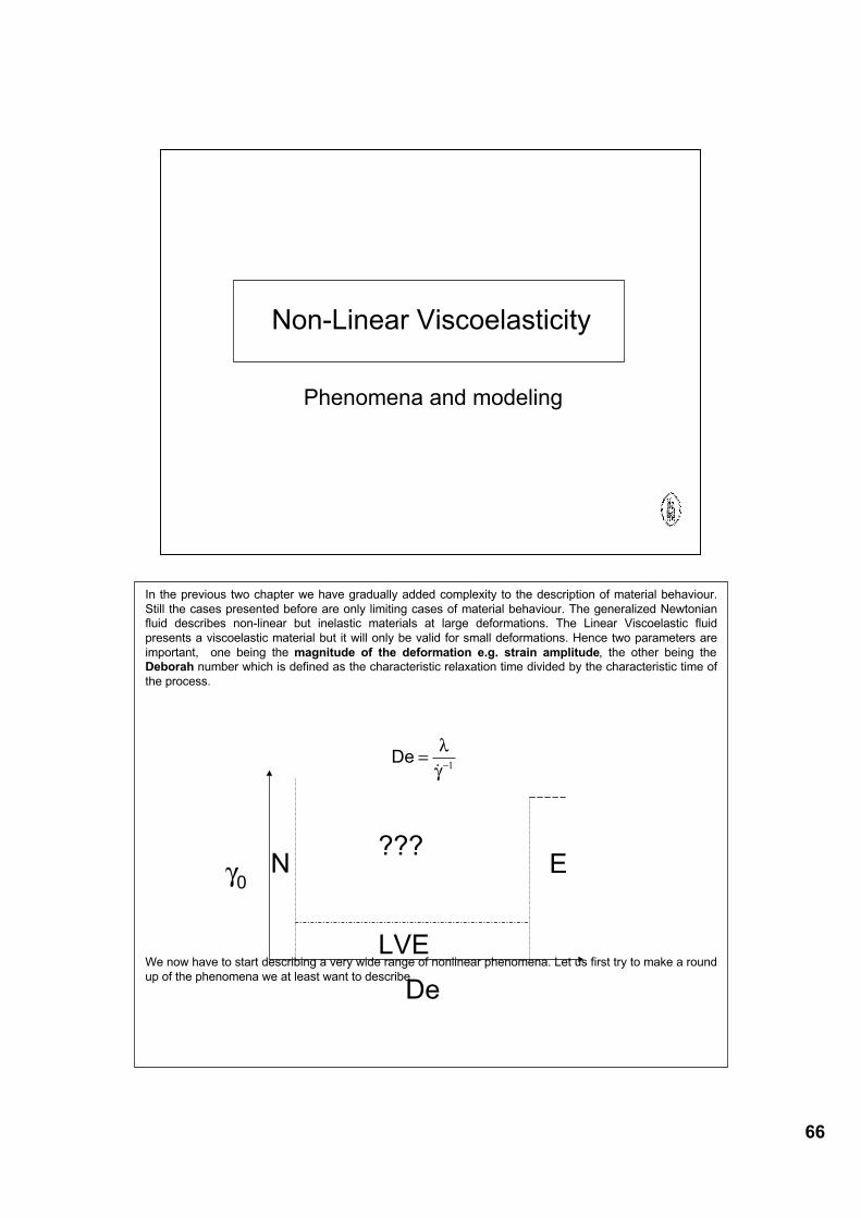
In the previous two chapter we have gradually added complexity to the description of material behaviour.Still the cases presented before are only limiting cases of material behaviour. The generalized Newtonianfluid describes non-linear but inelastic materials at large deformations. The Linear Viscoelastic fluidpresents a viscoelastic material but it will only be valid for small deformations. Hence two parameters areimportant, one being the magnitude of the deformation e.g. strain amplitude, the other being theDeborah number which is defined as the characteristic relaxation time divided by the characteristic time ofthe process.

We now have to start describing a very wide range of nonlinear phenomena. Let us first try to make a roundup of the phenomena we at least want to describe

1!"

#=!

De

N E

De

γ0

LVE

???

67

1. Non-linear VE phenomena

2. Additional mathematical tools

3. The second-order fluid

4. Quasi-linear models

5. Non-linear models

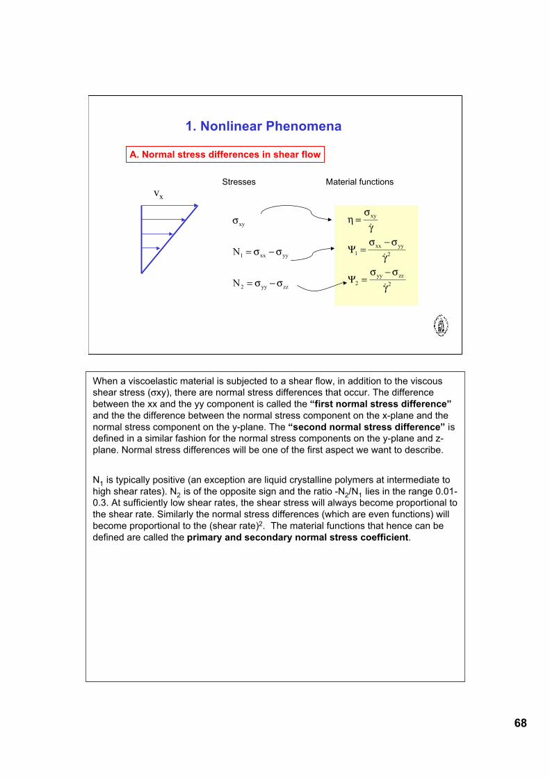
68

1. Nonlinear Phenomena

A. Normal stress differences in shear flow

2

zzyy

2

2

yyxx

1

xy

!

"#"=$

!

"#"=$

!

"=%

!

!

!

zzyy2

yyxx1

xy

N

N

!"!=

!"!=

!

Stresses Material functionsvx

When a viscoelastic material is subjected to a shear flow, in addition to the viscousshear stress (σxy), there are normal stress differences that occur. The differencebetween the xx and the yy component is called the “first normal stress difference”and the the difference between the normal stress component on the x-plane and thenormal stress component on the y-plane. The “second normal stress difference” isdefined in a similar fashion for the normal stress components on the y-plane and z-plane. Normal stress differences will be one of the first aspect we want to describe.

N1 is typically positive (an exception are liquid crystalline polymers at intermediate tohigh shear rates). N2 is of the opposite sign and the ratio -N2/N1 lies in the range 0.01-0.3. At sufficiently low shear rates, the shear stress will always become proportional tothe shear rate. Similarly the normal stress differences (which are even functions) willbecome proportional to the (shear rate)2. The material functions that hence can bedefined are called the primary and secondary normal stress coefficient.

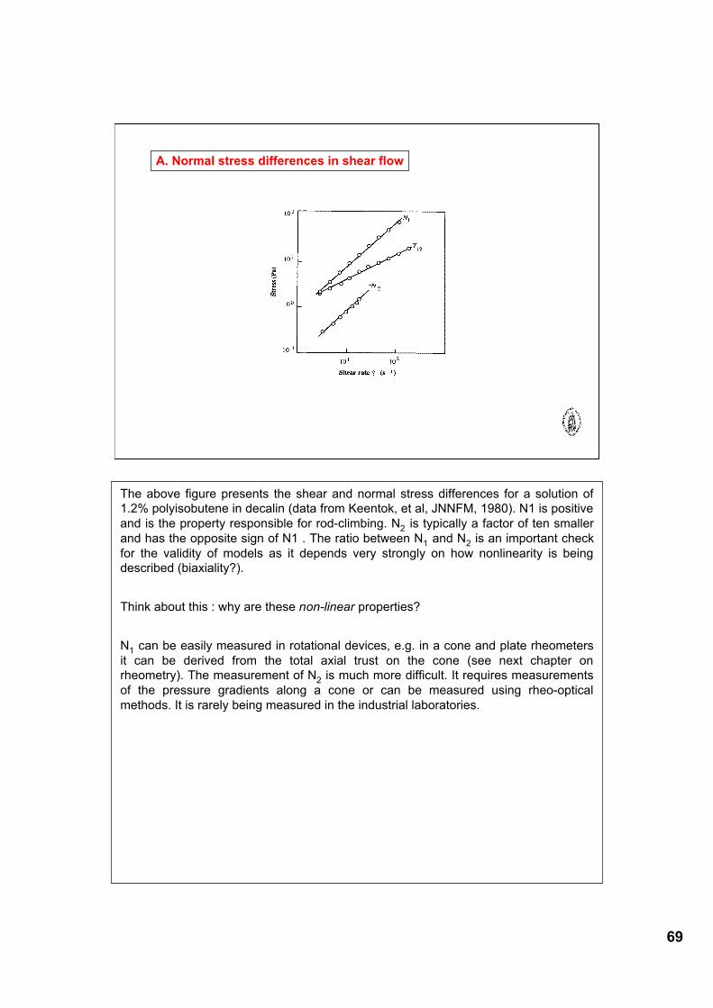
69

A. Normal stress differences in shear flow

The above figure presents the shear and normal stress differences for a solution of1.2% polyisobutene in decalin (data from Keentok, et al, JNNFM, 1980). N1 is positiveand is the property responsible for rod-climbing. N2 is typically a factor of ten smallerand has the opposite sign of N1 . The ratio between N1 and N2 is an important checkfor the validity of models as it depends very strongly on how nonlinearity is beingdescribed (biaxiality?).

Think about this : why are these non-linear properties?

N1 can be easily measured in rotational devices, e.g. in a cone and plate rheometersit can be derived from the total axial trust on the cone (see next chapter onrheometry). The measurement of N2 is much more difficult. It requires measurementsof the pressure gradients along a cone or can be measured using rheo-opticalmethods. It is rarely being measured in the industrial laboratories.

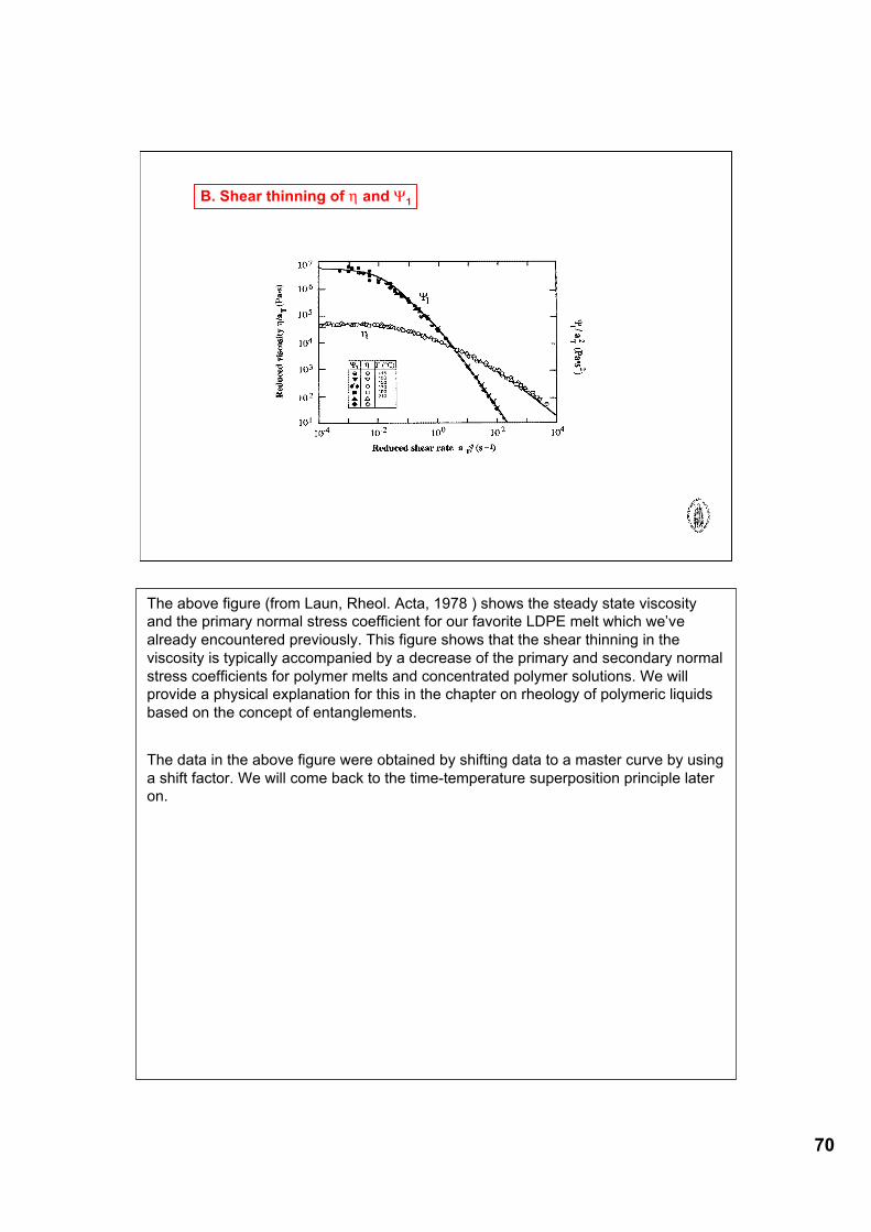
70

B. Shear thinning of η and Ψ1

The above figure (from Laun, Rheol. Acta, 1978 ) shows the steady state viscosityand the primary normal stress coefficient for our favorite LDPE melt which we’vealready encountered previously. This figure shows that the shear thinning in theviscosity is typically accompanied by a decrease of the primary and secondary normalstress coefficients for polymer melts and concentrated polymer solutions. We willprovide a physical explanation for this in the chapter on rheology of polymeric liquidsbased on the concept of entanglements.

The data in the above figure were obtained by shifting data to a master curve by usinga shift factor. We will come back to the time-temperature superposition principle lateron.

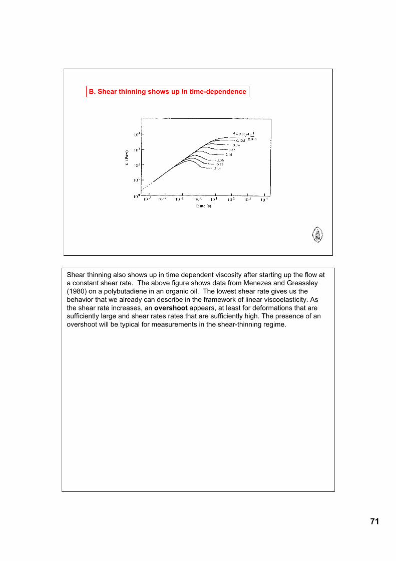
71

B. Shear thinning shows up in time-dependence

Shear thinning also shows up in time dependent viscosity after starting up the flow ata constant shear rate. The above figure shows data from Menezes and Greassley(1980) on a polybutadiene in an organic oil. The lowest shear rate gives us thebehavior that we already can describe in the framework of linear viscoelasticity. Asthe shear rate increases, an overshoot appears, at least for deformations that aresufficiently large and shear rates rates that are sufficiently high. The presence of anovershoot will be typical for measurements in the shear-thinning regime.

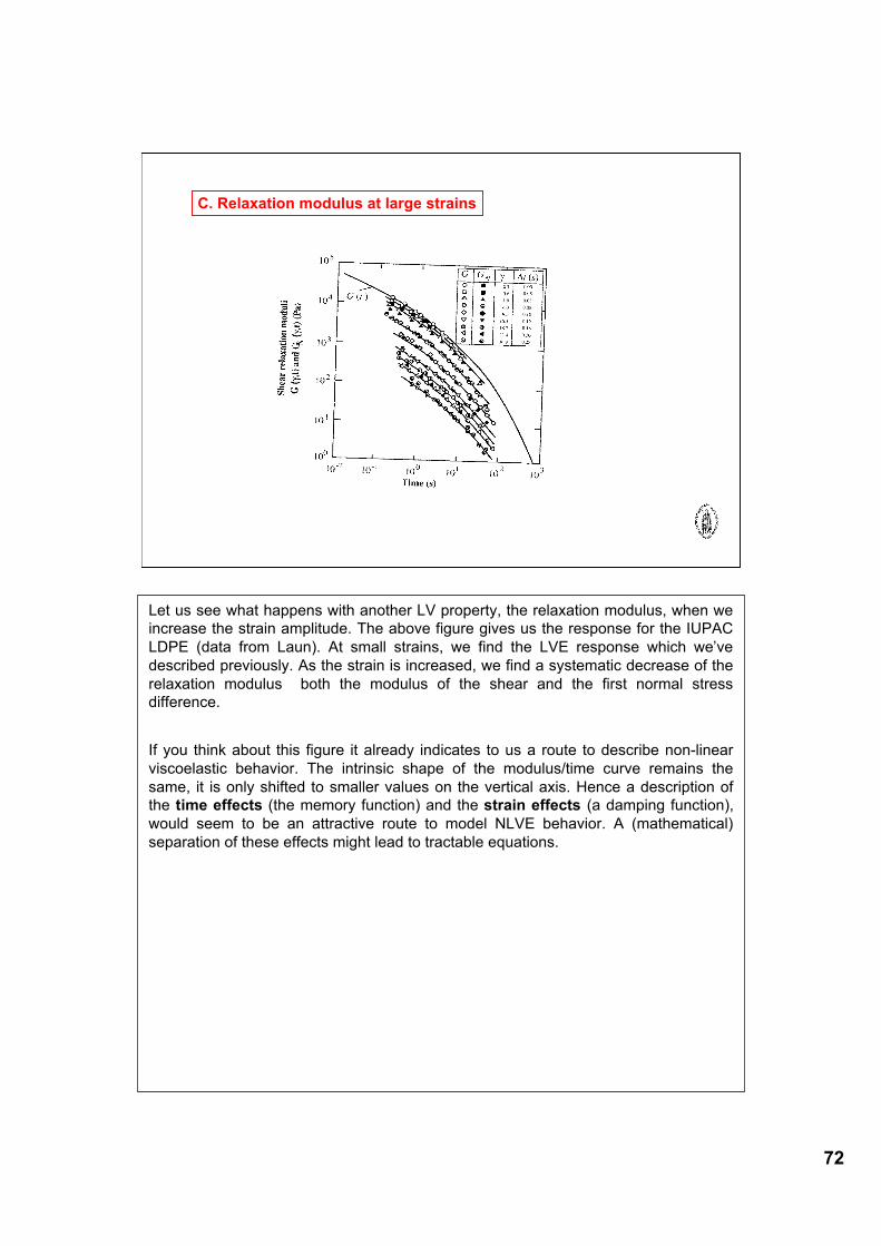
72

C. Relaxation modulus at large strains

Let us see what happens with another LV property, the relaxation modulus, when weincrease the strain amplitude. The above figure gives us the response for the IUPACLDPE (data from Laun). At small strains, we find the LVE response which we’vedescribed previously. As the strain is increased, we find a systematic decrease of therelaxation modulus both the modulus of the shear and the first normal stressdifference.

If you think about this figure it already indicates to us a route to describe non-linearviscoelastic behavior. The intrinsic shape of the modulus/time curve remains thesame, it is only shifted to smaller values on the vertical axis. Hence a description ofthe time effects (the memory function) and the strain effects (a damping function),would seem to be an attractive route to model NLVE behavior. A (mathematical)separation of these effects might lead to tractable equations.

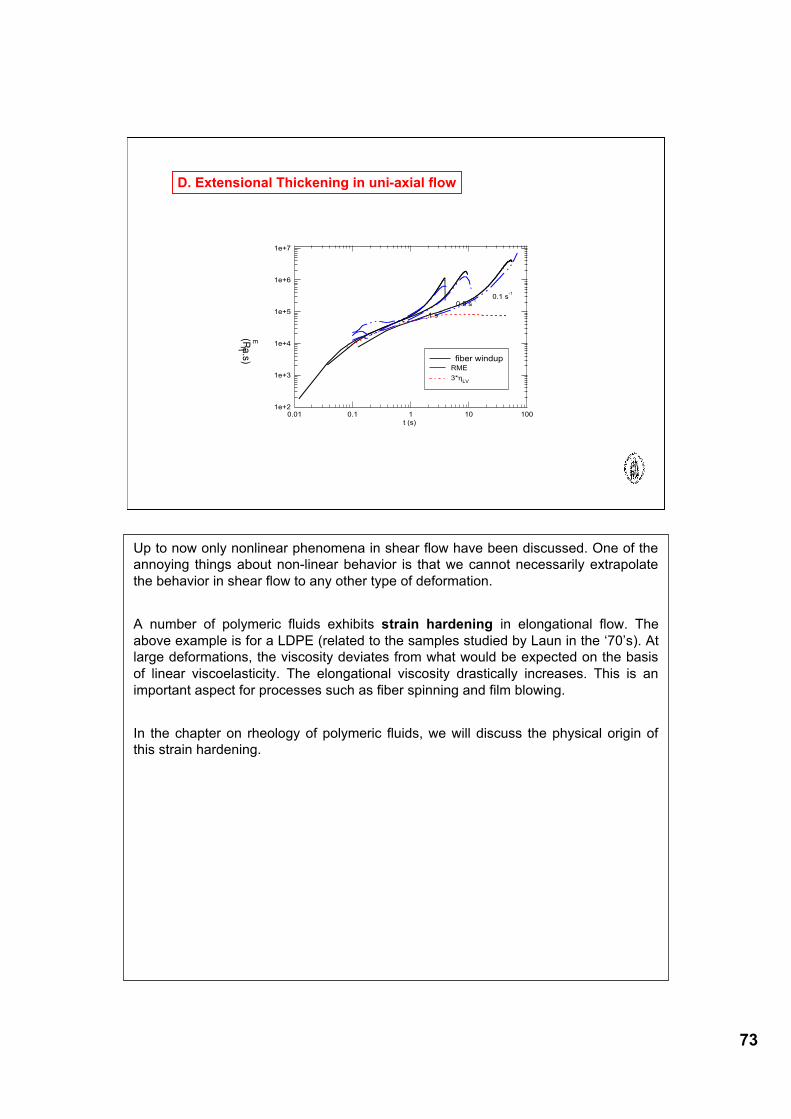
73

D. Extensional Thickening in uni-axial flow

t (s)

0.01 0.1 1 10 100

!

E

(Pa

.s)

1e+2

1e+3

1e+4

1e+5

1e+6

1e+7

fiber windupRME

3*!LV

0.1 s-1

0.5 s-1

1 s-1

Up to now only nonlinear phenomena in shear flow have been discussed. One of theannoying things about non-linear behavior is that we cannot necessarily extrapolatethe behavior in shear flow to any other type of deformation.

A number of polymeric fluids exhibits strain hardening in elongational flow. Theabove example is for a LDPE (related to the samples studied by Laun in the ‘70’s). Atlarge deformations, the viscosity deviates from what would be expected on the basisof linear viscoelasticity. The elongational viscosity drastically increases. This is animportant aspect for processes such as fiber spinning and film blowing.

In the chapter on rheology of polymeric fluids, we will discuss the physical origin ofthis strain hardening.

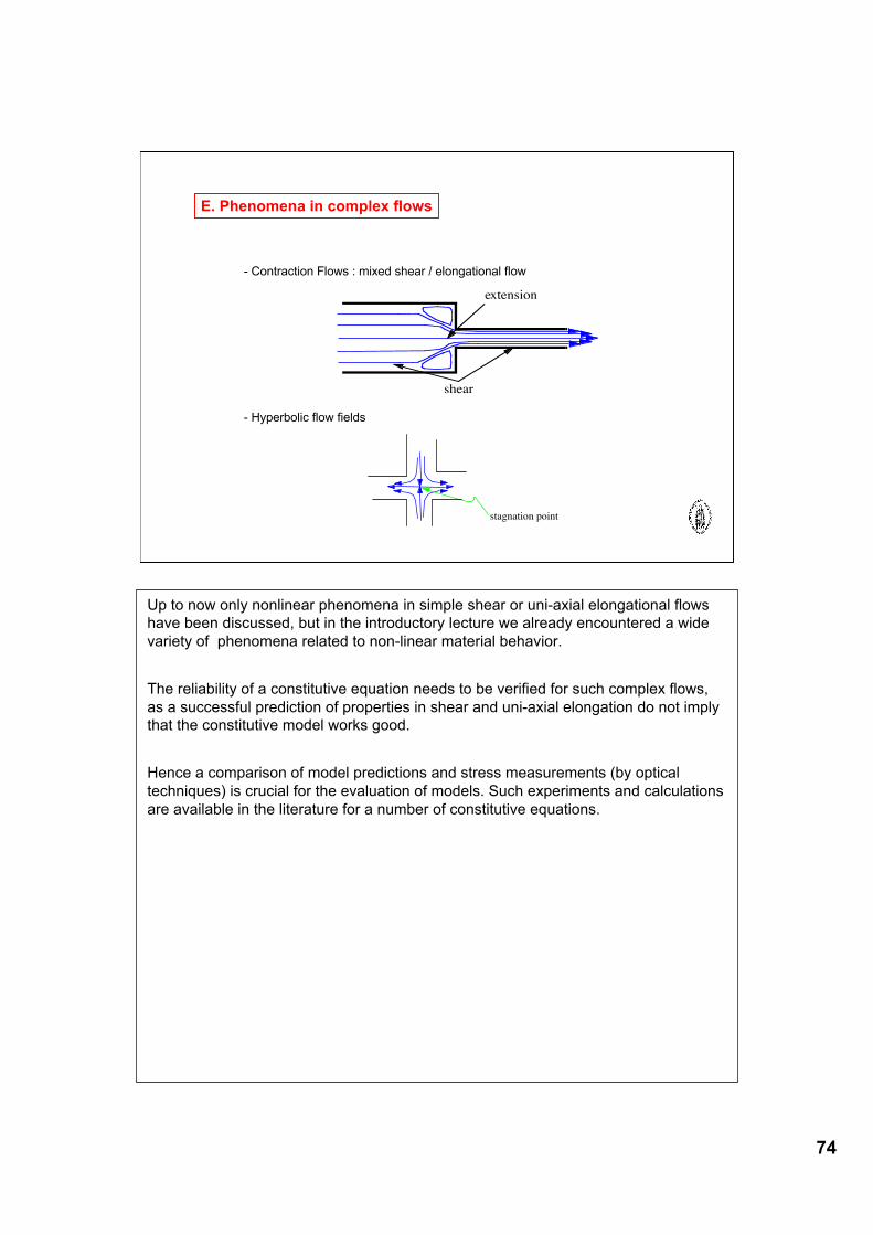
74

E. Phenomena in complex flows

- Contraction Flows : mixed shear / elongational flow

- Hyperbolic flow fields

shear

extension

stagnation point

Up to now only nonlinear phenomena in simple shear or uni-axial elongational flowshave been discussed, but in the introductory lecture we already encountered a widevariety of phenomena related to non-linear material behavior.

The reliability of a constitutive equation needs to be verified for such complex flows,as a successful prediction of properties in shear and uni-axial elongation do not implythat the constitutive model works good.

Hence a comparison of model predictions and stress measurements (by opticaltechniques) is crucial for the evaluation of models. Such experiments and calculationsare available in the literature for a number of constitutive equations.

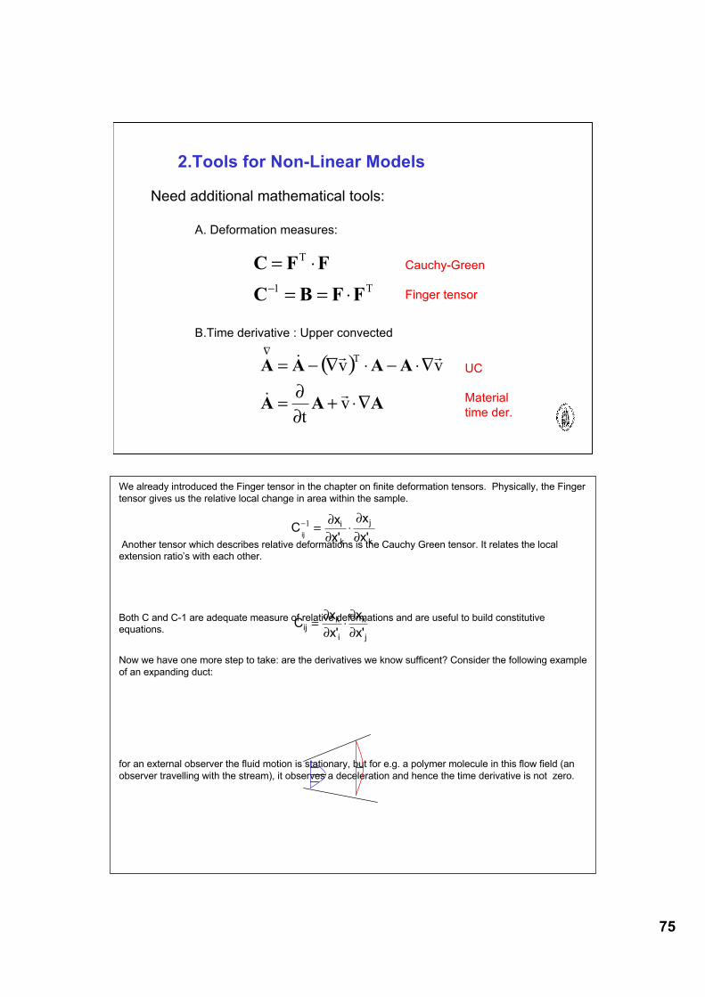
75

2.Tools for Non-Linear Models

Need additional mathematical tools:

A. Deformation measures:

B.Time derivative : Upper convected

T1

T

FFBC

FFC

!==

!=

"

Cauchy-GreenCauchy-Green

Finger tensorFinger tensor

( )

AAA

AAAA

!"+#

#=

!"$"!$=!

vt

vvT

!"

!!" UCUC

Material Material time der.time der.

We already introduced the Finger tensor in the chapter on finite deformation tensors. Physically, the Fingertensor gives us the relative local change in area within the sample.

Another tensor which describes relative deformations is the Cauchy Green tensor. It relates the localextension ratio’s with each other.

Both C and C-1 are adequate measure of relative deformations and are useful to build constitutiveequations.

Now we have one more step to take: are the derivatives we know sufficent? Consider the following exampleof an expanding duct:

for an external observer the fluid motion is stationary, but for e.g. a polymer molecule in this flow field (anobserver travelling with the stream), it observes a deceleration and hence the time derivative is not zero.

Cx

x

x

xij

i

k

j

k

!= "

1 #

#

#

#' '

Cx

x

x

xij

k

i

k

j

= !"

"

"

"' '

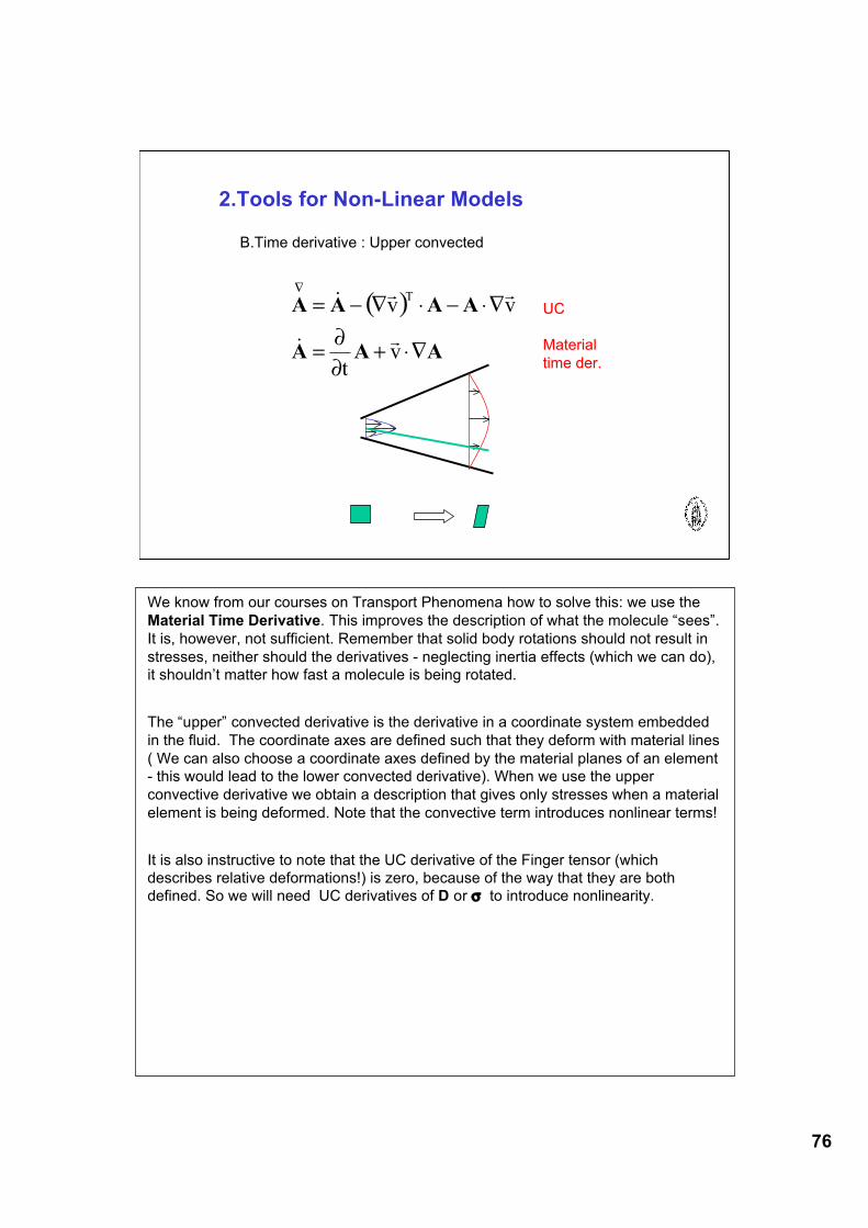
76

2.Tools for Non-Linear Models

B.Time derivative : Upper convected

( )

AAA

AAAA

!"+#

#=

!"$"!$=!

vt

vvT

!"

!!" UCUC

Material Material time der.time der.

We know from our courses on Transport Phenomena how to solve this: we use theMaterial Time Derivative. This improves the description of what the molecule “sees”.It is, however, not sufficient. Remember that solid body rotations should not result instresses, neither should the derivatives - neglecting inertia effects (which we can do),it shouldn’t matter how fast a molecule is being rotated.

The “upper” convected derivative is the derivative in a coordinate system embeddedin the fluid. The coordinate axes are defined such that they deform with material lines( We can also choose a coordinate axes defined by the material planes of an element- this would lead to the lower convected derivative). When we use the upperconvective derivative we obtain a description that gives only stresses when a materialelement is being deformed. Note that the convective term introduces nonlinear terms!

It is also instructive to note that the UC derivative of the Finger tensor (whichdescribes relative deformations!) is zero, because of the way that they are bothdefined. So we will need UC derivatives of D or σ to introduce nonlinearity.

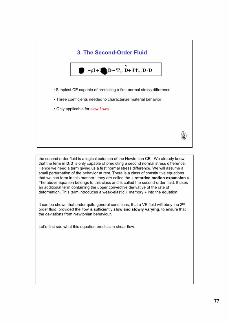
77

3. The Second-Order Fluid

DDDDI !"+"#+#=

$

0,20,1O 42p %&

• Simplest CE capable of predicting a first normal stress difference

• Three coefficients needed to characterize material behavior

• Only applicable for slow flows

the second order fluid is a logical extenion of the Newtonian CE. We already knowthat the term in D.D is only capable of predicting a second normal stress difference.Hence we need a term giving us a first normal stress difference. We will assume asmall perturbation of the behavior at rest. There is a class of constitutive equationsthat we can form in this manner : they are called the « retarded motion expansion ».The above equation belongs to this class and is called the second-order fluid. It usesan additional term containing the upper convective derivative of the rate ofdeformation. This term introduces a weak-elastic « memory » into the equation.

It can be shown that under quite general conditions, that a VE fluid will obey the 2nd

order fluid, provided the flow is sufficiently slow and slowly varying, to ensure thatthe deviations from Newtonian behaviour.

Let’s first see what this equation predicts in shear flow.

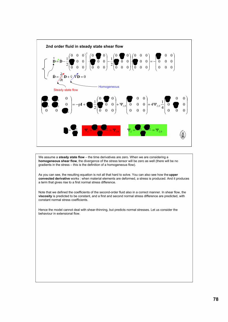
78

0vt

000

000

00

000

00

000

000

00

00

2

1

000

00

00

000

00

000

2

1

2T

=!"+##

=

$$$

%

&

'''

(

)

*=

$$$

%

&

'''

(

)"

$$$

%

&

'''

(

)*

$$$

%

&

'''

(

)"

$$$

%

&

'''

(

)*=

!

DDD

DD

!"

"

""

"

"

"

""

+++

++

++

Steady state flowHomogeneous

2nd order fluid in steady state shear flow

!!!

"

#

$$$

%

&

'+

!!!

"

#

$$$

%

&

'+!!!

"

#

$$$

%

&+(=

!!!

"

#

$$$

%

&

000

00

00

4

14

000

000

00

000

00

00

2

12p

00

0

02

2

0,2

2

0,10

zz

yyyx

xyxx

)))

))

*+

++++

!

!!

!

!

I

0,22

zzyy

20,12

yyxx

1

xy

0 !="

=!!="

=!=#

$$

#

$$

#

$%

!!!

We assume a steady state flow – the time derivatives are zero. When we are considering ahomogeneous shear flow, the divergence of the stress tensor will be zero as well (there will be nogradients in the stress – this is the definition of a homogeneous flow).

As you can see, the resulting equation is not all that hard to solve. You can also see how the upperconvected derivative works : when material elements are deformed, a stress is produced. And it producesa term that gives rise to a first normal stress difference.

Note that we defined the coefficients of the second-order fluid also in a correct manner. In shear flow, theviscosity is predicted to be constant, and a first and second normal stress difference are predicted, withconstant normal stress coefficients.

Hence the model cannot deal with shear-thinning, but predicts normal stresses. Let us consider thebehaviour in extensional flow.

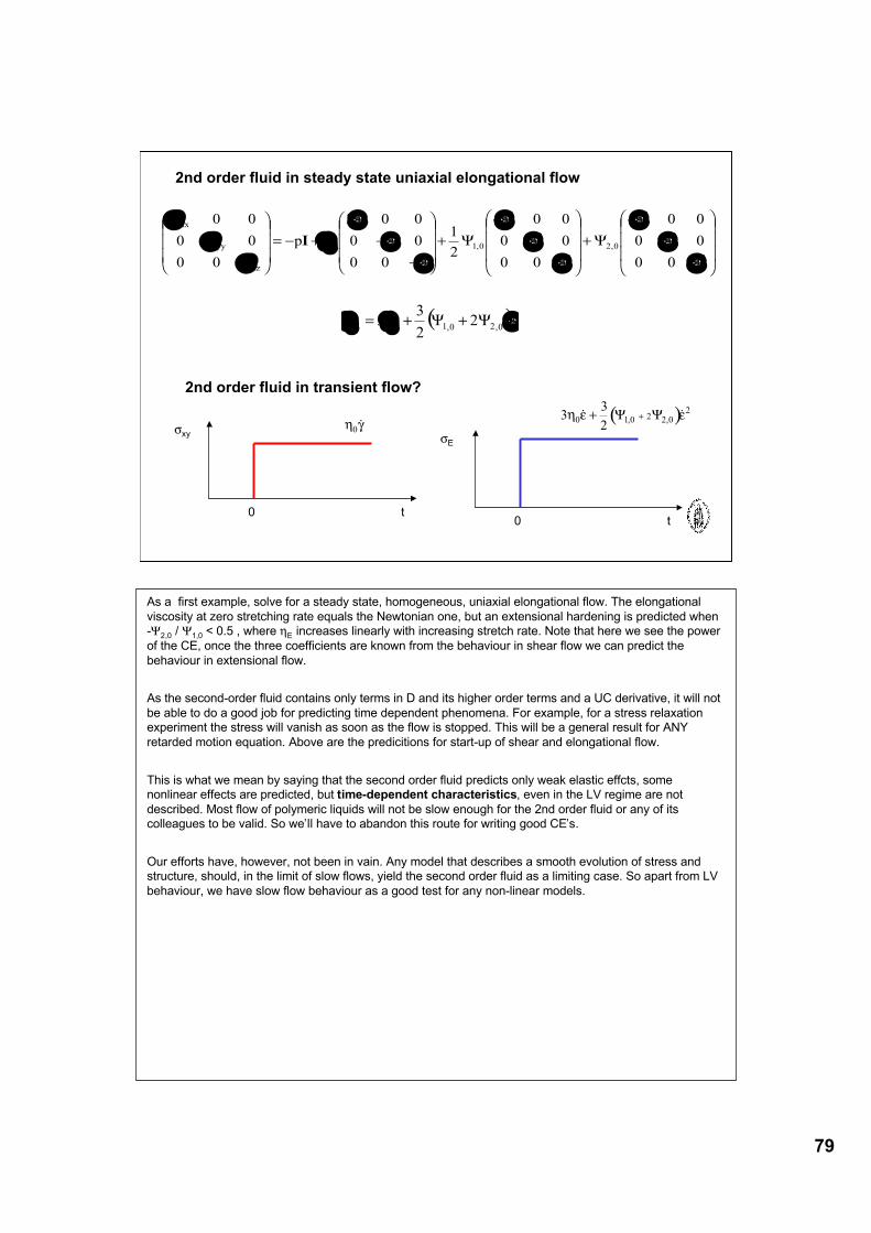
79

2nd order fluid in steady state uniaxial elongational flow

!!!

"

#

$$$

%

&

'+!!!

"

#

$$$

%

&

'+

!!!

"

#

$$$

%

&

((+(=

!!!

"

#

$$$

%

&

2

2

2

0,2

2

2

2

0,10

zz

yy

xx

00

00

004

00

00

004

2

1

00

00

002

p

00

00

00

))

)

))

)

))

)*

++

+

!

!

!

!

!

!

!

!

!

I

( )!"" !0,20,10E

22

33 #+#+=

2nd order fluid in transient flow?

σxy

t0

σE

t0

! "0!

( )33

20 1 0

22 0

2! " "! !

, ,+ +# #

As a first example, solve for a steady state, homogeneous, uniaxial elongational flow. The elongationalviscosity at zero stretching rate equals the Newtonian one, but an extensional hardening is predicted when-Ψ2,0 / Ψ1,0 < 0.5 , where ηE increases linearly with increasing stretch rate. Note that here we see the powerof the CE, once the three coefficients are known from the behaviour in shear flow we can predict thebehaviour in extensional flow.

As the second-order fluid contains only terms in D and its higher order terms and a UC derivative, it will notbe able to do a good job for predicting time dependent phenomena. For example, for a stress relaxationexperiment the stress will vanish as soon as the flow is stopped. This will be a general result for ANYretarded motion equation. Above are the predicitions for start-up of shear and elongational flow.

This is what we mean by saying that the second order fluid predicts only weak elastic effcts, somenonlinear effects are predicted, but time-dependent characteristics, even in the LV regime are notdescribed. Most flow of polymeric liquids will not be slow enough for the 2nd order fluid or any of itscolleagues to be valid. So we’ll have to abandon this route for writing good CE’s.

Our efforts have, however, not been in vain. Any model that describes a smooth evolution of stress andstructure, should, in the limit of slow flows, yield the second order fluid as a limiting case. So apart from LVbehaviour, we have slow flow behaviour as a good test for any non-linear models.

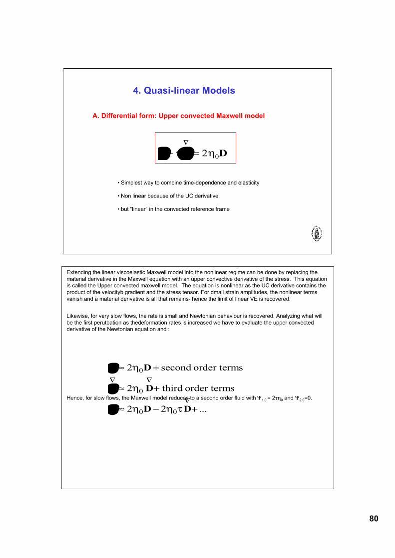
80

4. Quasi-linear Models

A. Differential form: Upper convected Maxwell model

! !+ =

"

# $20D

• Simplest way to combine time-dependence and elasticity

• Non linear because of the UC derivative

• but “linear” in the convected reference frame

Extending the linear viscoelastic Maxwell model into the nonlinear regime can be done by replacing thematerial derivative in the Maxwell equation with an upper convective derivative of the stress. This equationis called the Upper convected maxwell model. The equation is nonlinear as the UC derivative contains theproduct of the velocityb gradient and the stress tensor. For dmall strain amplitudes, the nonlinear termsvanish and a material derivative is all that remains- hence the limit of linear VE is recovered.

Likewise, for very slow flows, the rate is small and Newtonian behaviour is recovered. Analyzing what willbe the first perutbation as thedeformation rates is increased we have to evaluate the upper convectedderivative of the Newtonian equation and :

Hence, for slow flows, the Maxwell model reduces to a second order fluid with Ψ1,0 = 2τη0 and Ψ2,0=0.

...22

sorder term third2

sorder term second 2

00

0

0

+!"#"$

+"$

+"$

%

%%

DD

D

D

&

&

&

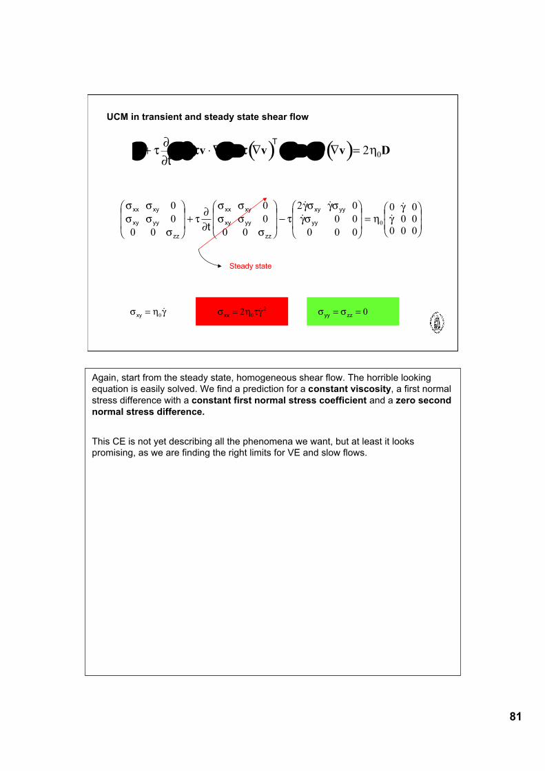
81

UCM in transient and steady state shear flow

( ) ( )! ! + ! " ! " !+ #$ $ # # $ =%&

&% % % '

t

T

v v v D20

! !! !

!"##

! !! !

!"

$! $!$! %

$$

xx xy

xy yy

zz

xx xy

xy yy

zz

xy yy

yyt

0

0

0 0

0

0

0 0

2 0

0 0

0 0 0

0 0

0 0

0 0 0

0

&

'

((

)

*

++ +

&

'

((

)

*

++ ,

&

'

((

)

*

++ =

&

'((

)

*++

! !

!

!

!

Steady state

! " # ! " $# ! !xy xx yy zz= = = =

0 0

22 0! !

Again, start from the steady state, homogeneous shear flow. The horrible lookingequation is easily solved. We find a prediction for a constant viscosity, a first normalstress difference with a constant first normal stress coefficient and a zero secondnormal stress difference.

This CE is not yet describing all the phenomena we want, but at least it lookspromising, as we are finding the right limits for VE and slow flows.

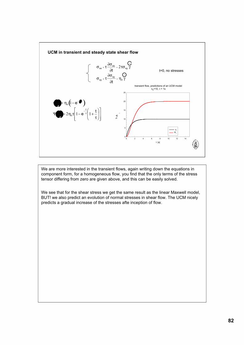
82

transient flow, predictions of an UCM model

!0=10, " = 1s

t [s]

0 2 4 6 8 10 12 14

!, #

1

0

5

10

15

20

25

!

#1

UCM in transient and steady state shear flow

! "#!

#"! $

! "#!

#% $

xxxx

xy

xy

xy

t

t

+ =

+ =

2

0

.

.t=0, no stresses

( )! !

! ""

"

"

( )

( )

/t e

t et

t

t

= #

= # +$

%&

'

()

*

+,,

-

.//

#

#

0

1 0

1

2 1 10

We are more interested in the transient flows, again writing down the equations incomponent form, for a homogeneous flow, you find that the only terms of the stresstensor differing from zero are given above, and this can be easily solved.

We see that for the shear stress we get the same result as the linear Maxwell model,BUT! we also predict an evolution of normal stresses in shear flow. The UCM nicelypredicts a gradual increase of the stresses afte inception of flow.

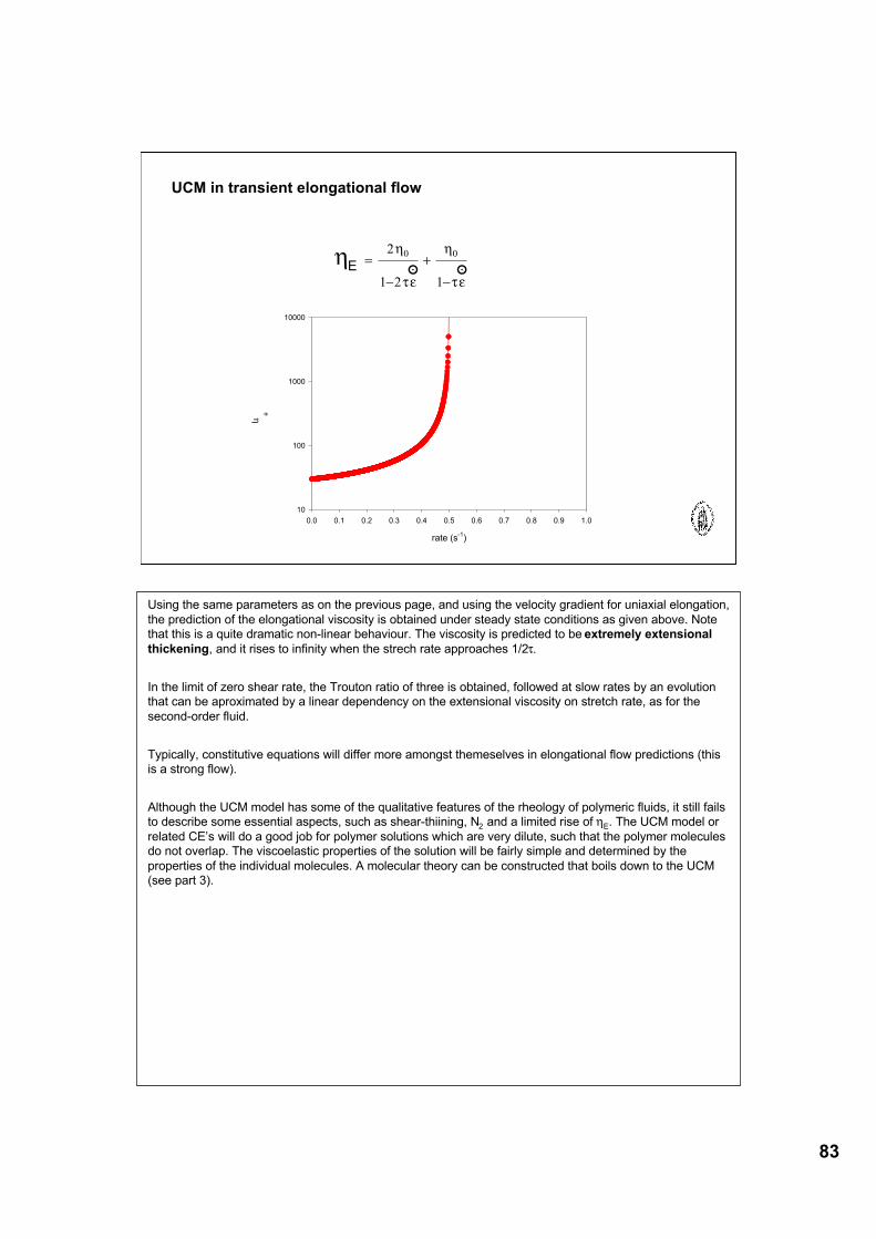
83

rate (s-1

)

0.0 0.1 0.2 0.3 0.4 0.5 0.6 0.7 0.8 0.9 1.0

!

e

10

100

1000

10000

UCM in transient elongational flow

!!

"#

!

"#

E=

$

+

$

2

1 2 1

0 0

. .

Using the same parameters as on the previous page, and using the velocity gradient for uniaxial elongation,the prediction of the elongational viscosity is obtained under steady state conditions as given above. Notethat this is a quite dramatic non-linear behaviour. The viscosity is predicted to be extremely extensionalthickening, and it rises to infinity when the strech rate approaches 1/2τ.

In the limit of zero shear rate, the Trouton ratio of three is obtained, followed at slow rates by an evolutionthat can be aproximated by a linear dependency on the extensional viscosity on stretch rate, as for thesecond-order fluid.

Typically, constitutive equations will differ more amongst themeselves in elongational flow predictions (thisis a strong flow).

Although the UCM model has some of the qualitative features of the rheology of polymeric fluids, it still failsto describe some essential aspects, such as shear-thiining, N2 and a limited rise of ηE. The UCM model orrelated CE’s will do a good job for polymer solutions which are very dilute, such that the polymer moleculesdo not overlap. The viscoelastic properties of the solution will be fairly simple and determined by theproperties of the individual molecules. A molecular theory can be constructed that boils down to the UCM(see part 3).

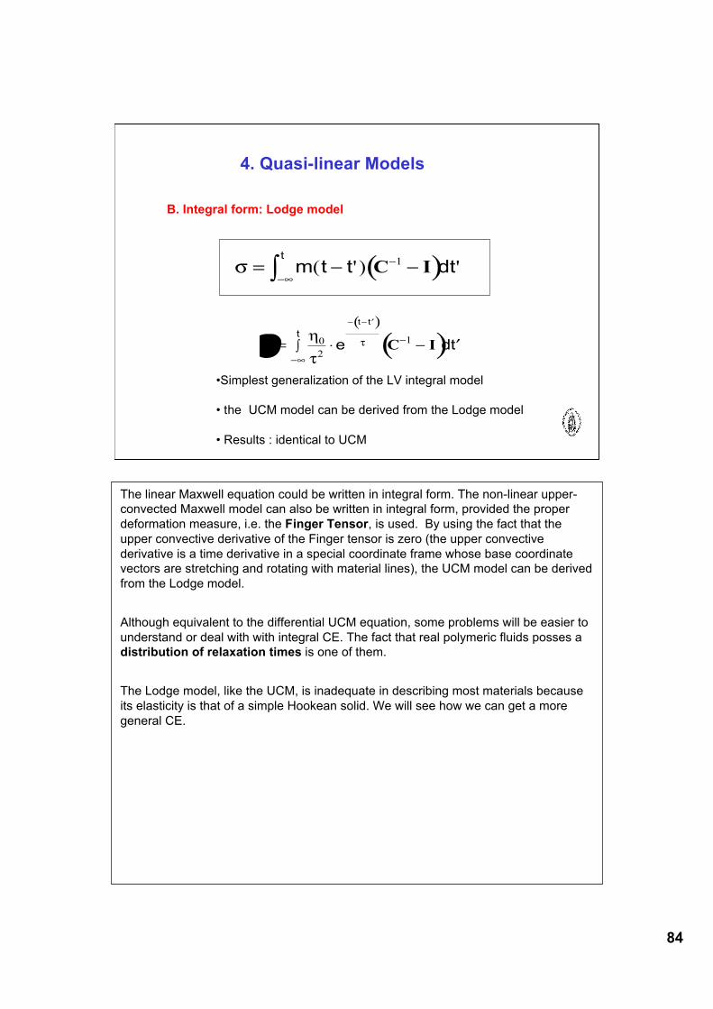
84

4. Quasi-linear Models

B. Integral form: Lodge model

( )

( )! = " # $#%

#&

# # $

'

((0

2

1t

e dt

t t

C I

•Simplest generalization of the LV integral model

• the UCM model can be derived from the Lodge model

• Results : identical to UCM

( )! = " ""#

"

$ m t t dtt

( ' ) 'C I1

The linear Maxwell equation could be written in integral form. The non-linear upper-convected Maxwell model can also be written in integral form, provided the properdeformation measure, i.e. the Finger Tensor, is used. By using the fact that theupper convective derivative of the Finger tensor is zero (the upper convectivederivative is a time derivative in a special coordinate frame whose base coordinatevectors are stretching and rotating with material lines), the UCM model can be derivedfrom the Lodge model.

Although equivalent to the differential UCM equation, some problems will be easier tounderstand or deal with with integral CE. The fact that real polymeric fluids posses adistribution of relaxation times is one of them.

The Lodge model, like the UCM, is inadequate in describing most materials becauseits elasticity is that of a simple Hookean solid. We will see how we can get a moregeneral CE.

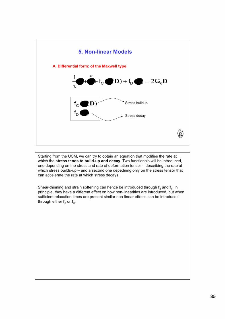
85

5. Non-linear Models

A. Differential form: of the Maxwell type

12 0

!" " " "+ + + =

#

f f GC D( , ) ( )D D

f

f

C

D

( , )

( )

!

!

D Stress buildup

Stress decay

Starting from the UCM, we can try to obtain an equation that modifies the rate atwhich the stress tends to build-up and decay. Two functionals will be introduced,one depending on the stress and rate of deformation tensor - describing the rate atwhich stress builds-up – and a second one depedning only on the stress tensor thatcan accelerate the rate at which stress decays.

Shear-thinning and strain softening can hence be introduced through fc and fd. Inprinciple, they have a different effect on how non-linearities are introduced, but whensufficient relaxation times are present similar non-linear effects can be introducedthrough either fc or fd.

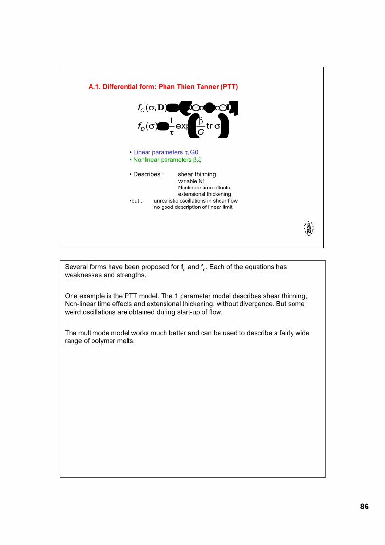
86

A.1. Differential form: Phan Thien Tanner (PTT)

( )

I

DDD

!"#

$%&

=

'+'=

()

*(

((+(

trexp)(

),(

Gf

f

D

C

1

• Linear parameters τ, G0• Nonlinear parameters β,ξ

• Describes : shear thinningvariable N1Nonlinear time effectsextensional thickening

•but : unrealistic oscillations in shear flowno good description of linear limit

Several forms have been proposed for fd and fc. Each of the equations hasweaknesses and strengths.

One example is the PTT model. The 1 parameter model describes shear thinning,Non-linear time effects and extensional thickening, without divergence. But someweird oscillations are obtained during start-up of flow.

The multimode model works much better and can be used to describe a fairly widerange of polymer melts.

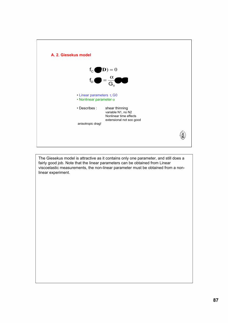
87

A. 2. Giesekus model

f

fG

C

D

( , )

( )

!

! ! !

D =

= "

0

0

#

• Linear parameters τ, G0• Nonlinear parameter α

• Describes : shear thinningvariable N1, no N2Nonlinear time effectsextensional not soo good

anisotropic drag!

The Giesekus model is attractive as it contains only one parameter, and still does afairly good job. Note that the linear parameters can be obtained from Linearviscoelastic measurements, the non-linear parameter must be obtained from a non-linear experiment.

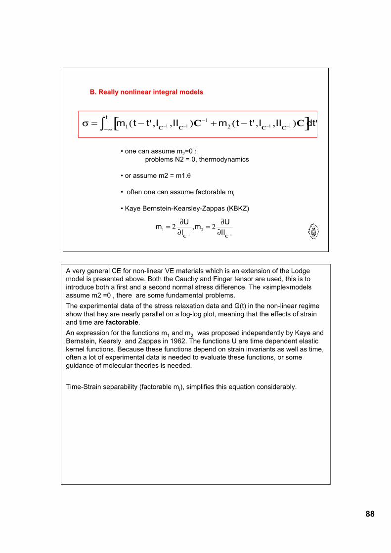
88

B. Really nonlinear integral models

• one can assume m2=0 : problems N2 = 0, thermodynamics

• or assume m2 = m1.θ

• often one can assume factorable mi

• Kaye Bernstein-Kearsley-Zappas (KBKZ)

[ ]! = " + "" " " "

"

"#$ m t t I II m t t I II dtt

1

1

21 1 1 1( ' , , ) ( ' , , ) 'C C C C

C C

mU

Im

U

II1 22 2

1 1

= =

! !

"

"

"

"C C

,

A very general CE for non-linear VE materials which is an extension of the Lodgemodel is presented above. Both the Cauchy and Finger tensor are used, this is tointroduce both a first and a second normal stress difference. The «simple»modelsassume m2 =0 , there are some fundamental problems.The experimental data of the stress relaxation data and G(t) in the non-linear regimeshow that hey are nearly parallel on a log-log plot, meaning that the effects of strainand time are factorable.An expression for the functions m1 and m2 was proposed independently by Kaye andBernstein, Kearsly and Zappas in 1962. The functions U are time dependent elastickernel functions. Because these functions depend on strain invariants as well as time,often a lot of experimental data is needed to evaluate these functions, or someguidance of molecular theories is needed.

Time-Strain separability (factorable mi), simplifies this equation considerably.

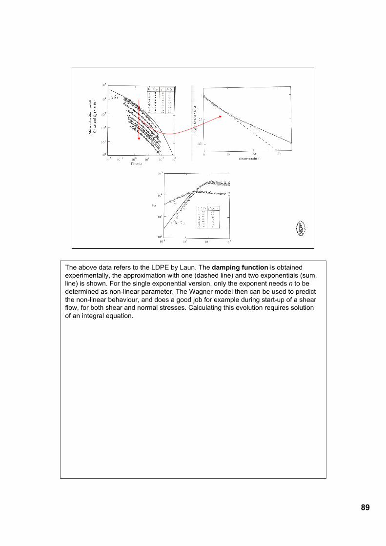
89

The above data refers to the LDPE by Laun. The damping function is obtainedexperimentally, the approximation with one (dashed line) and two exponentials (sum,line) is shown. For the single exponential version, only the exponent needs n to bedetermined as non-linear parameter. The Wagner model then can be used to predictthe non-linear behaviour, and does a good job for example during start-up of a shearflow, for both shear and normal stresses. Calculating this evolution requires solutionof an integral equation.

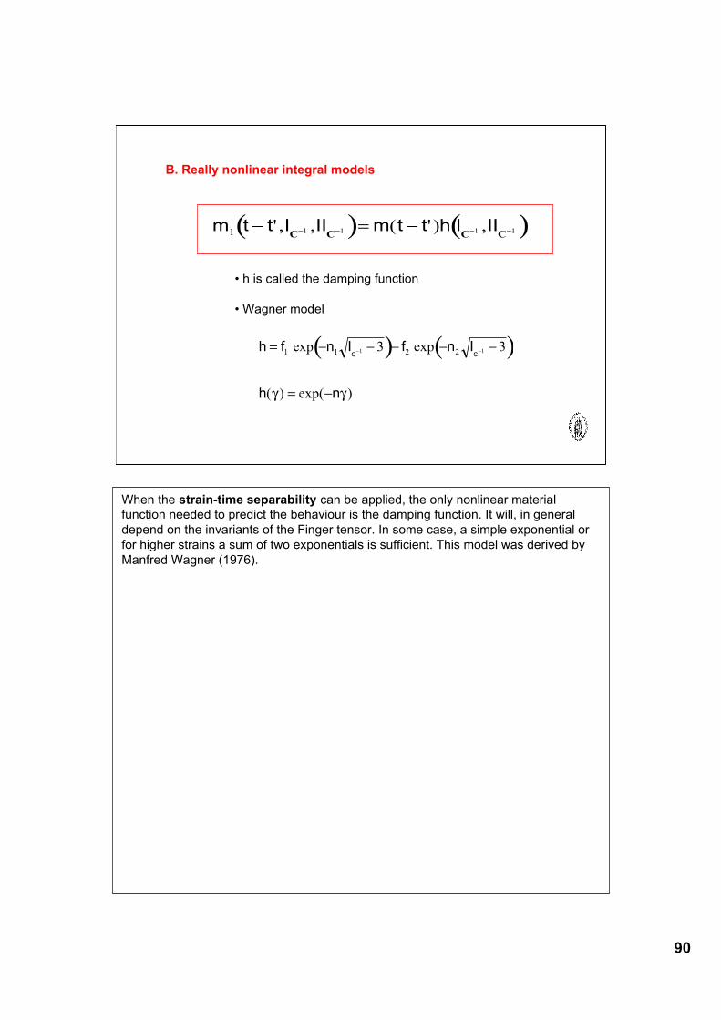
90

B. Really nonlinear integral models

• h is called the damping function

• Wagner model

( ) ( )m t t I II m t t h I II1 1 1 1 1! = !! ! ! !' , , ( ' ) ,C C C C

( ) ( )h f n I f n I

h n

c c= ! ! ! ! !

= !

! !1 1 2 21 13 3exp exp

( ) exp( )" "

When the strain-time separability can be applied, the only nonlinear materialfunction needed to predict the behaviour is the damping function. It will, in generaldepend on the invariants of the Finger tensor. In some case, a simple exponential orfor higher strains a sum of two exponentials is sufficient. This model was derived byManfred Wagner (1976).

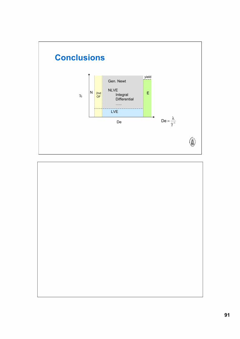
91

N E

De

γ0

LVE

2ndOF

Gen. Newt

NLVEIntegralDifferential…..

Conclusions

yield

1!"

#=!

De

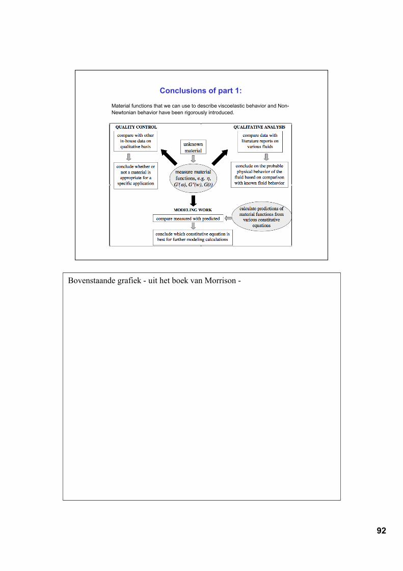
92

Conclusions of part 1:

Material functions that we can use to describe viscoelastic behavior and Non-Newtonian behavior have been rigorously introduced.

Bovenstaande grafiek - uit het boek van Morrison -

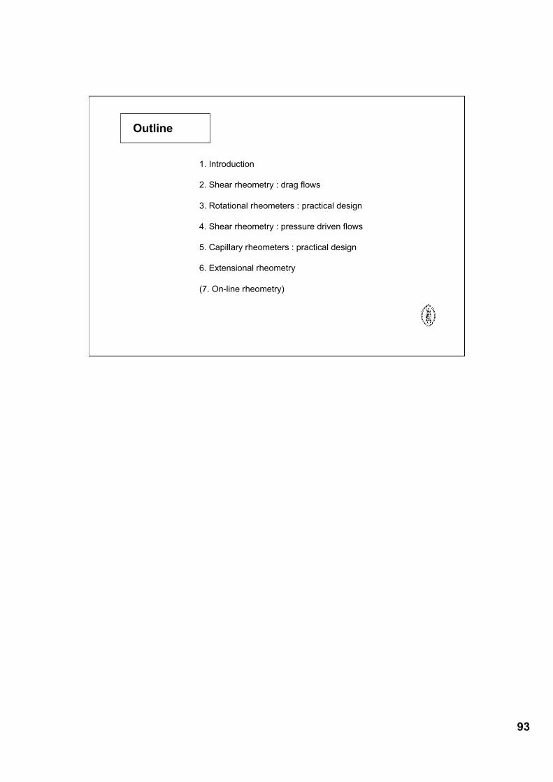
93

Outline

1. Introduction

2. Shear rheometry : drag flows

3. Rotational rheometers : practical design

4. Shear rheometry : pressure driven flows

5. Capillary rheometers : practical design

6. Extensional rheometry

(7. On-line rheometry)

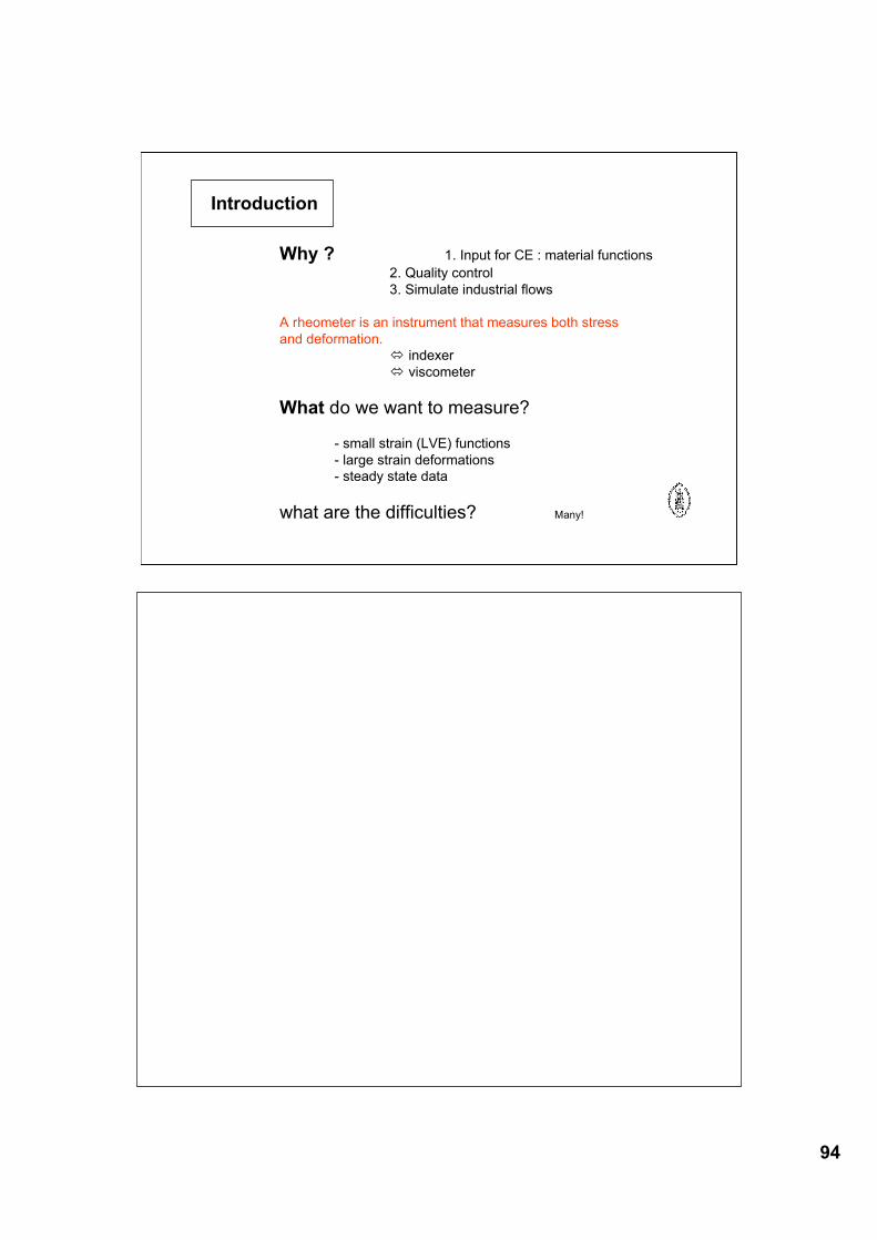
94

Introduction

Why ? 1. Input for CE : material functions2. Quality control3. Simulate industrial flows

A rheometer is an instrument that measures both stress and deformation.

indexer viscometer

What do we want to measure?

- small strain (LVE) functions- large strain deformations- steady state data

what are the difficulties? Many!

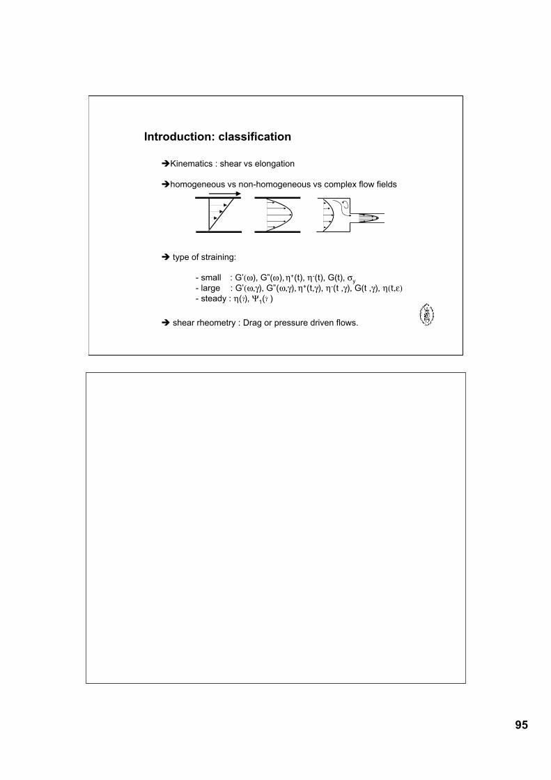
95

Introduction: classification

Kinematics : shear vs elongation

homogeneous vs non-homogeneous vs complex flow fields

type of straining:

- small : G’(ω), G”(ω), η+(t), η-(t), G(t), σy- large : G’(ω,γ), G”(ω,γ), η+(t,γ), η-(t ,γ), G(t ,γ), η(t,ε)- steady : η( ), Ψ1( )

shear rheometry : Drag or pressure driven flows.

!! !!

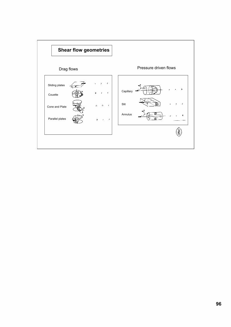
96

Shear flow geometries

Sliding plates

Couette

Cone and Plate

Parallel plates

Drag flows Pressure driven flows

Capillary

Slit

Annulus

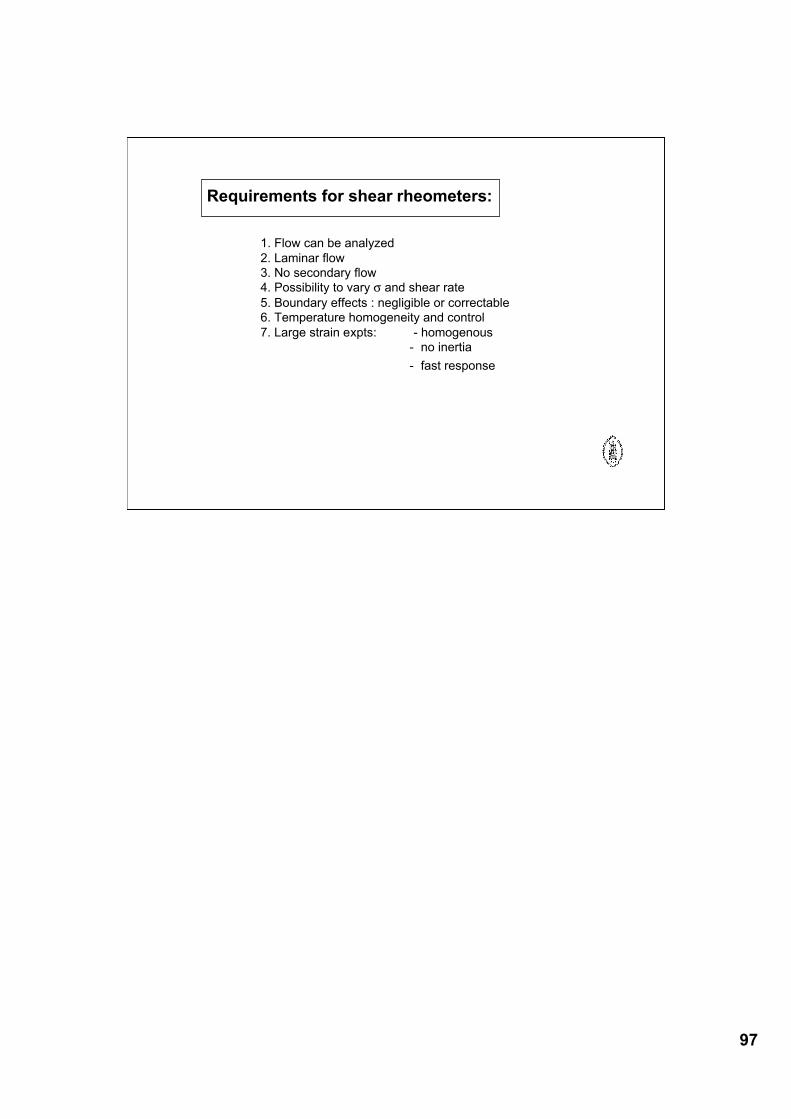
97

Requirements for shear rheometers:

1. Flow can be analyzed2. Laminar flow3. No secondary flow4. Possibility to vary σ and shear rate5. Boundary effects : negligible or correctable6. Temperature homogeneity and control 7. Large strain expts: - homogenous

- no inertia- fast response

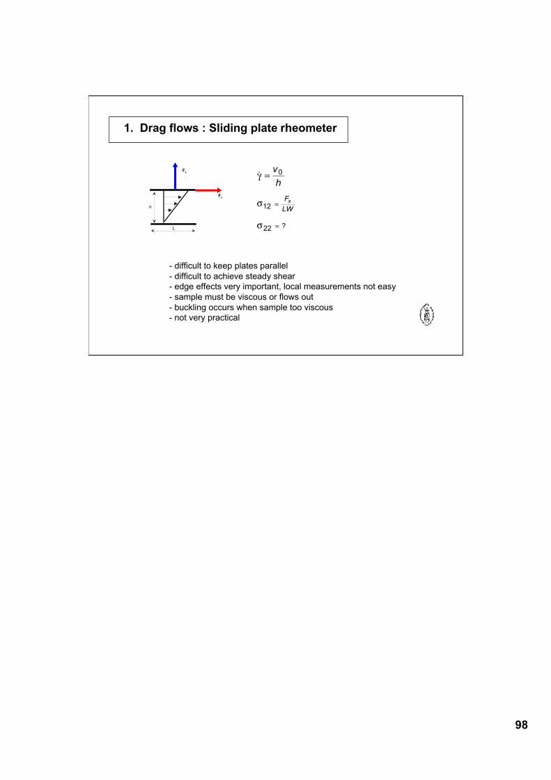
98

1. Drag flows : Sliding plate rheometer

Fy

Fx

h

L

!

?

!

"

"

=

=

=

v

h

F

LW

x

0

12

22

- difficult to keep plates parallel- difficult to achieve steady shear - edge effects very important, local measurements not easy- sample must be viscous or flows out- buckling occurs when sample too viscous- not very practical

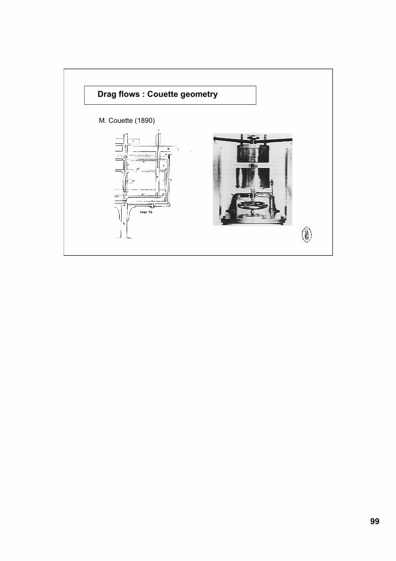
99

Drag flows : Couette geometry

M. Couette (1890)

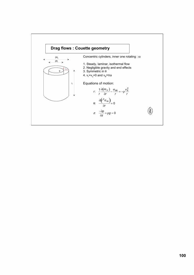
100

Drag flows : Couette geometry

2R0

2Ri

L

Concentric cylinders, inner one rotating : ω

1. Steady, laminar, isothermal flow2. Negligible gravity and end effects3. Symmetric in θ4. vr=vz=0 and vθ=rω

Equations of motion:

( )

( )

rr

r

r r

v

r

r

r

zp

zg

rr

r

:

:

:

1

0

0

2

2

! "

!

"#

$! "

!

!

!#

$$ $

$

% = %

=

%+ =

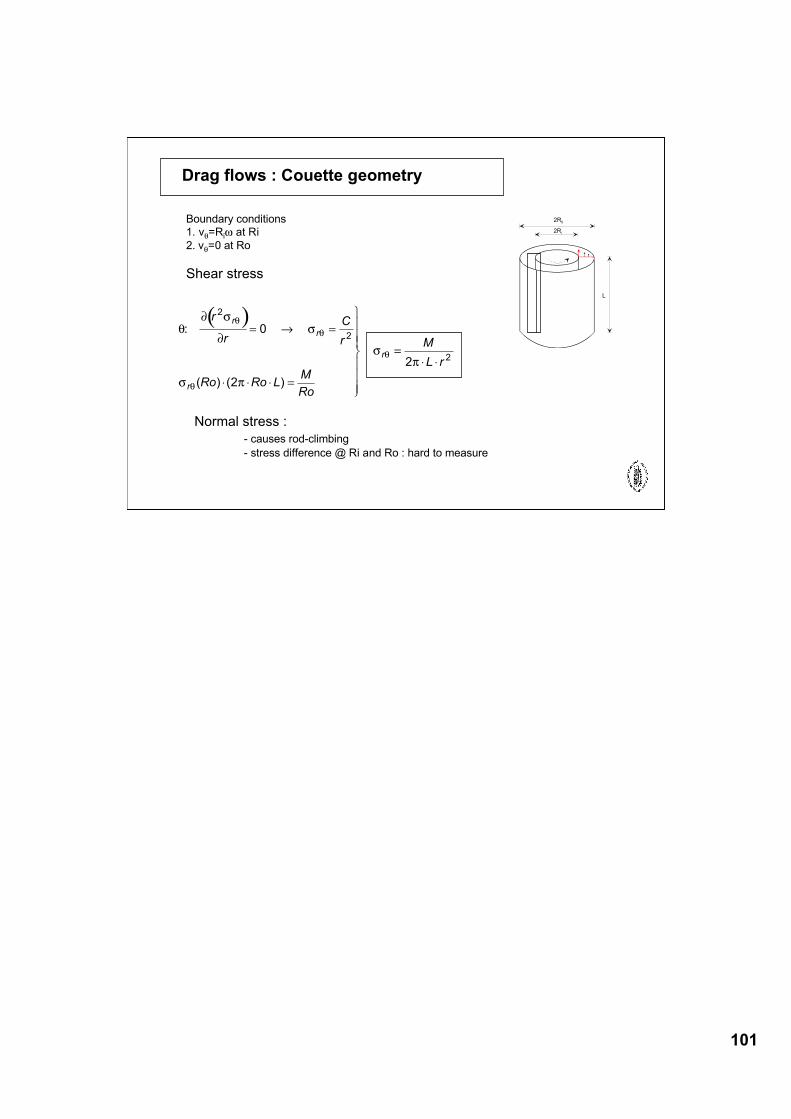
101

Drag flows : Couette geometry

2R0

2Ri

L

Boundary conditions1. vθ=Riω at Ri2. vθ=0 at Ro

Shear stress

( )!

" #

"#

# $

#$

!

!

!

!

:

( ) ( )

r

r

C

r

Ro Ro LM

Ro

M

L r

r

r

r

r

2

2

2

0

2

2

= % =

& & & =

'

(

)))

*

)))

=& &

Normal stress : - causes rod-climbing- stress difference @ Ri and Ro : hard to measure

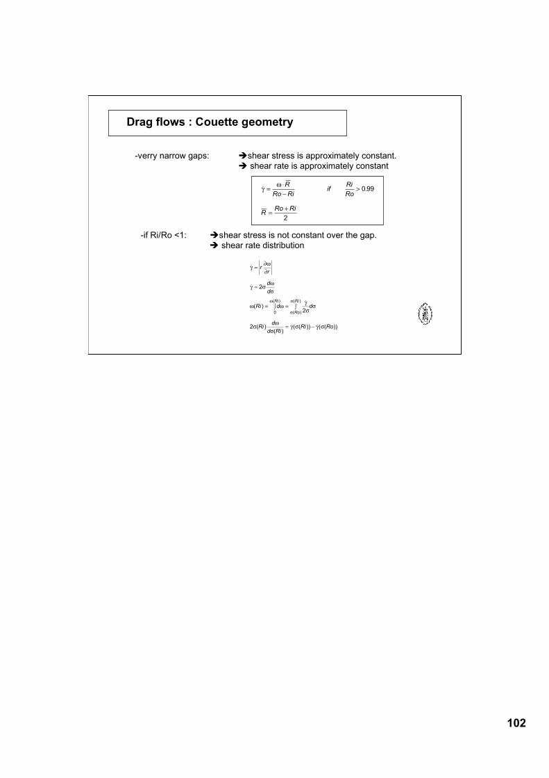
102

Drag flows : Couette geometry

-verry narrow gaps: shear stress is approximately constant. shear rate is approximately constant

! .!"

=#

$>

=+

R

Ro Riif

Ri

Ro

RRo Ri

0 99

2

-if Ri/Ro <1: shear stress is not constant over the gap. shear rate distribution

!

!

( )!

( )( )

!( ( )) !( ( ))

( )

( )

( )

!"#"

! $#$

# #!$

$

$#

$! $ ! $

#

$

$

=

=

= % = %

= &

rr

d

d

Ri d d

Rid

d RiRi Ro

Ri

Ro

Ri

2

2

2

0

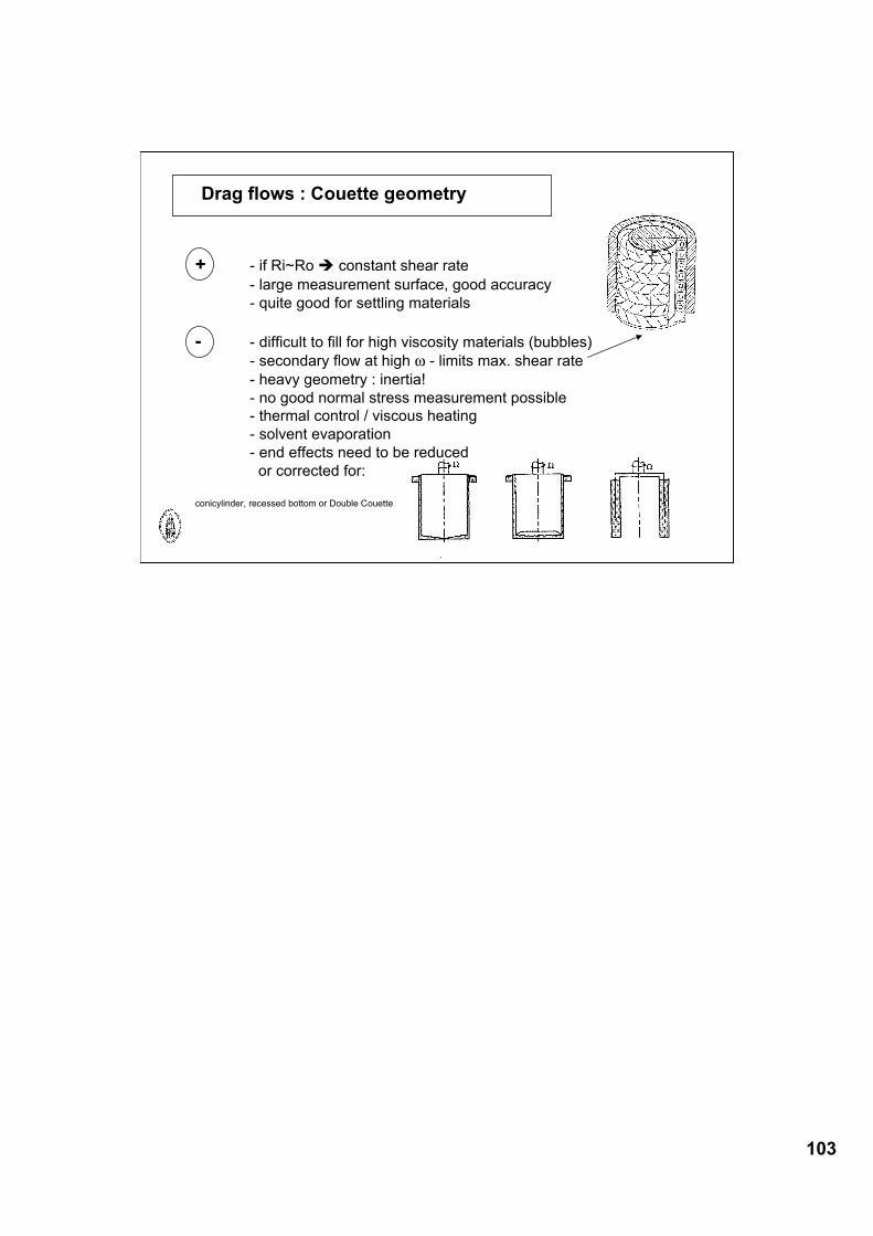
103

Drag flows : Couette geometry

+ - if Ri~Ro constant shear rate- large measurement surface, good accuracy- quite good for settling materials

- - difficult to fill for high viscosity materials (bubbles)- secondary flow at high ω - limits max. shear rate- heavy geometry : inertia!- no good normal stress measurement possible- thermal control / viscous heating - solvent evaporation- end effects need to be reduced or corrected for:

conicylinder, recessed bottom or Double Couette

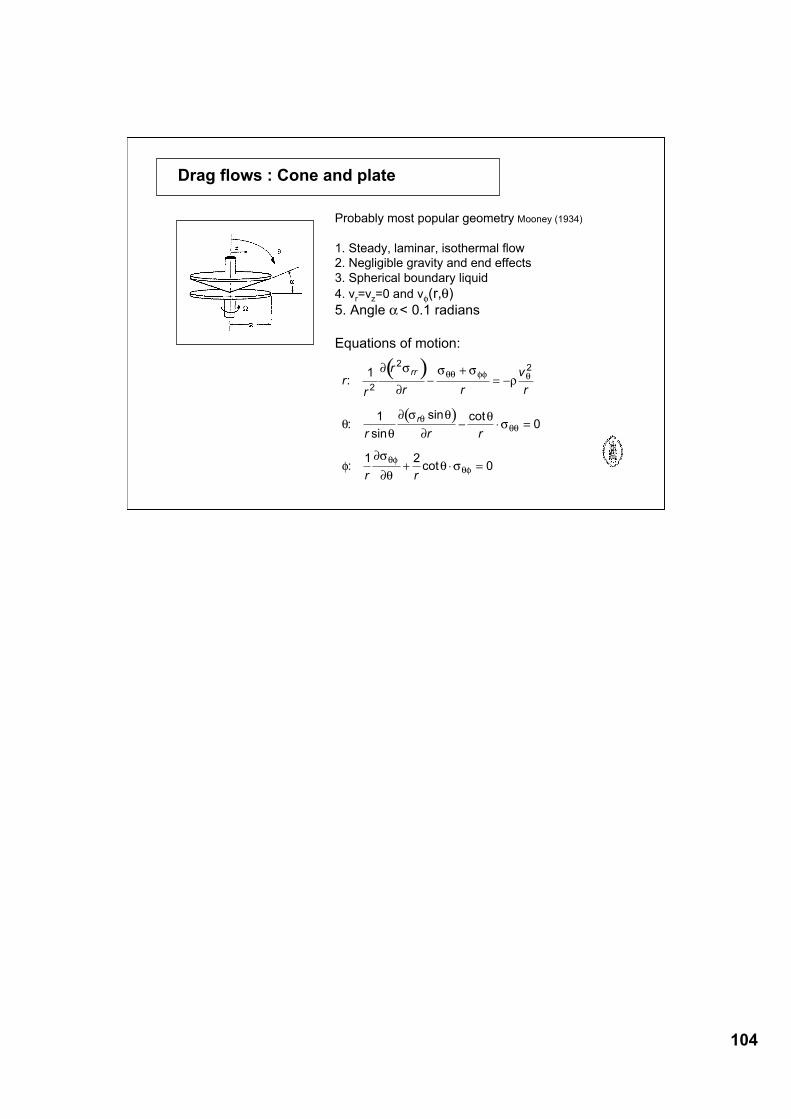
104

Drag flows : Cone and plate

( )

( )

r

r

r

r r

v

r

r r r

r r

rr

r

:

:sin

sin cot

: cot

1

10

1 20

2

22! "

!

" "#

$$

! " $

!

$"

%!"

!$$ "

$$ %% $

$$$

$%$%

&+

= &

& ' =

+ ' =

Probably most popular geometry Mooney (1934)

1. Steady, laminar, isothermal flow2. Negligible gravity and end effects3. Spherical boundary liquid4. vr=vz=0 and vφ(r,θ)5. Angle α < 0.1 radians

Equations of motion:

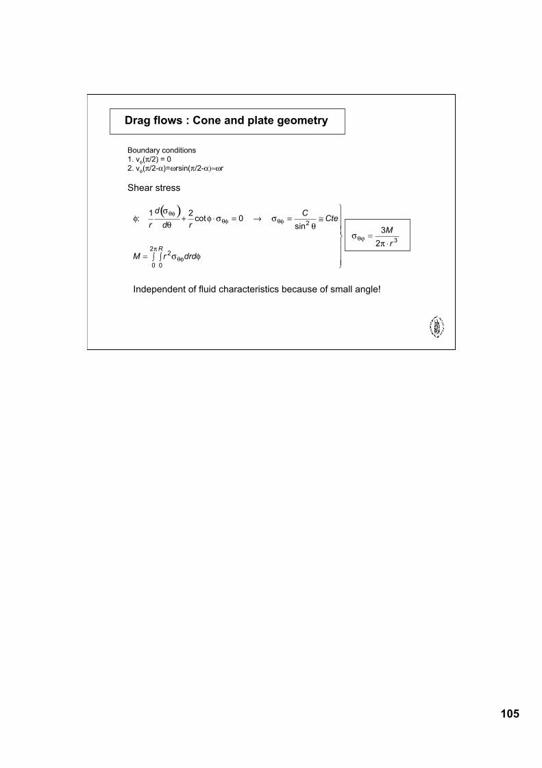
105

Drag flows : Cone and plate geometry

Boundary conditions1. vφ(π/2) = 02. vφ(π/2-α)=ωrsin(π/2-α)≈ωr

Shear stress

( )!

"

#! " "

#

" !

"$

#!#! #!

#!

$

#%

: cot

sin

1 20

3

2

2

2

00

2

3

r

d

d r

CCte

M r drd

M

rR

+ & = ' = (

= ))

*

+

,,,

-

,,,

=&

Independent of fluid characteristics because of small angle!

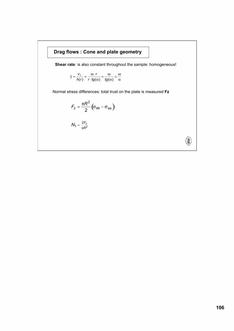
106

Drag flows : Cone and plate geometry

Normal stress differences: total trust on the plate is measured Fz

( )FR

N

z

F

R

z

= !

=

"# #$$ %%

"

2

1

2

2

2

Shear rate: is also constant throughout the sample: homogeneous!

!

( ) ( ) ( )!

"

#

"

#

"

#= =

$

$= %

v

h r

r

r tg tg

r

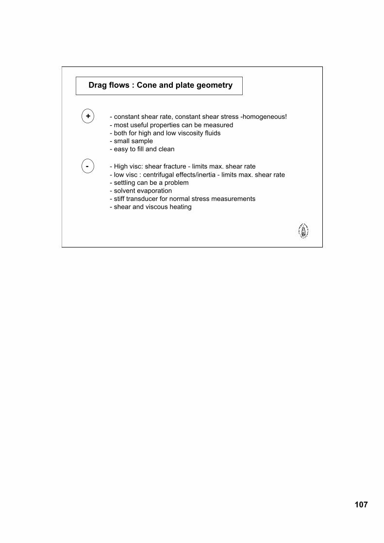
107

Drag flows : Cone and plate geometry

+ - constant shear rate, constant shear stress -homogeneous!- most useful properties can be measured- both for high and low viscosity fluids- small sample- easy to fill and clean

- - High visc: shear fracture - limits max. shear rate- low visc : centrifugal effects/inertia - limits max. shear rate- settling can be a problem- solvent evaporation- stiff transducer for normal stress measurements- shear and viscous heating

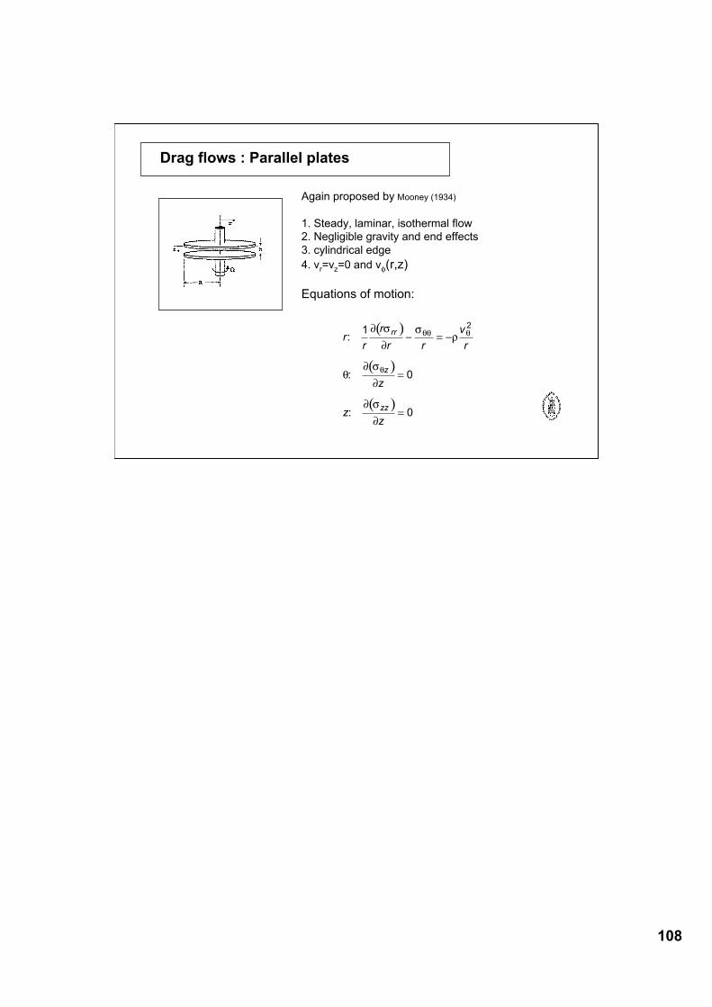
108

Drag flows : Parallel plates

Again proposed by Mooney (1934)

1. Steady, laminar, isothermal flow2. Negligible gravity and end effects3. cylindrical edge4. vr=vz=0 and vφ(r,z)

Equations of motion:

( )

( )

( )

rr

r

r r

v

r

z

zz

rr

z

zz

:

:

:

1

0

0

2! "

!

"#

$! "

!

! "

!

$$ $

$

% = %

=

=

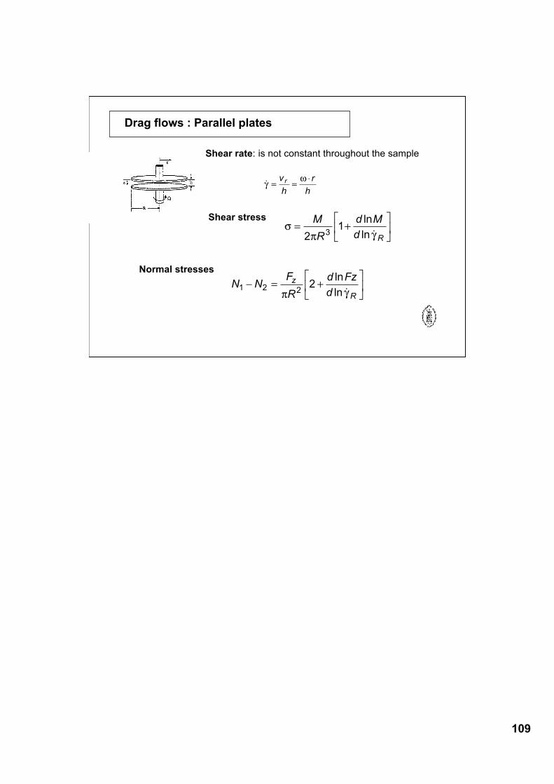
109

Drag flows : Parallel plates

Shear rate: is not constant throughout the sample

!!"

= =#v

h

r

h

r

Shear stress!

" #= +

$

%&

'

()

M

R

d M

d R2

13

ln

ln !

Normal stressesN N

F

R

d Fz

d

z

R

1 2 22! = +"

#$

%

&'

( )ln

ln !

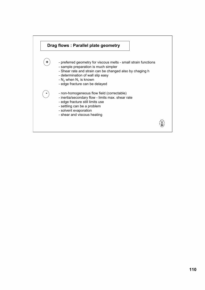
110

Drag flows : Parallel plate geometry

+ - preferred geometry for viscous melts - small strain functions- sample preparation is much simpler- Shear rate and strain can be changed also by chaging h- determination of wall slip easy- N2 when N1 is known- edge fracture can be delayed

- - non-homogeneous flow field (correctable)- inertia/secondary flow - limits max. shear rate- edge fracture still limits use- settling can be a problem- solvent evaporation- shear and viscous heating

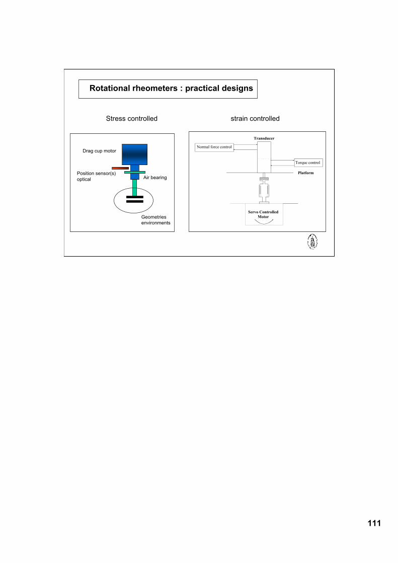
111

Rotational rheometers : practical designs

Stress controlled strain controlled

Transducer

Normal force control

Torque control

Platform

Servo Controlled

Motor

Drag cup motor

Position sensor(s)optical Air bearing

Geometriesenvironments

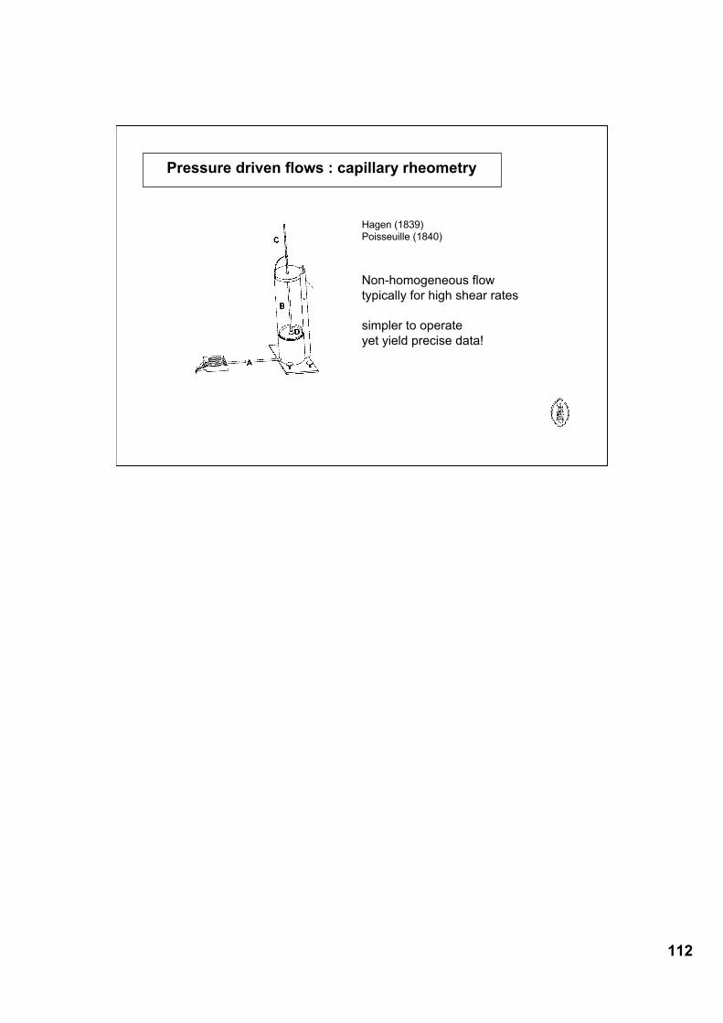
112

Pressure driven flows : capillary rheometry

Hagen (1839)Poisseuille (1840)

Non-homogeneous flowtypically for high shear rates

simpler to operateyet yield precise data!

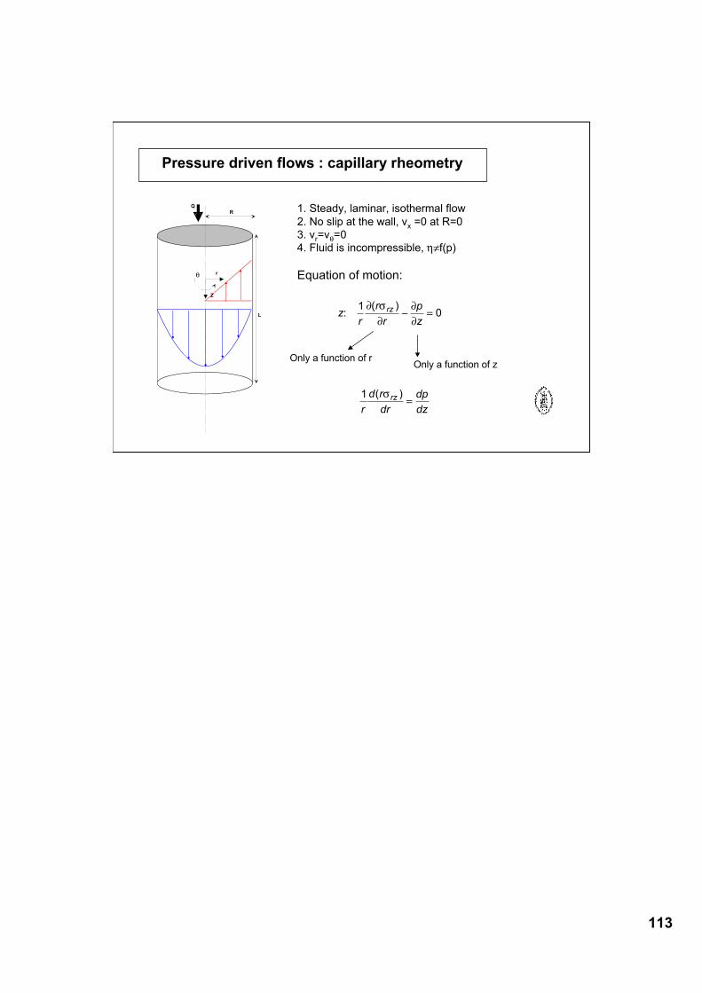
113

r

Z

!

L

R

Q

Pressure driven flows : capillary rheometry

1. Steady, laminar, isothermal flow2. No slip at the wall, vx =0 at R=03. vr=vθ=04. Fluid is incompressible, η≠f(p)

Equation of motion:

zr

r

r

p

z

rz:( )1

0! "

!

!

!# =

Only a function of zOnly a function of r

1

r

d r

dr

dp

dz

rz( )!=

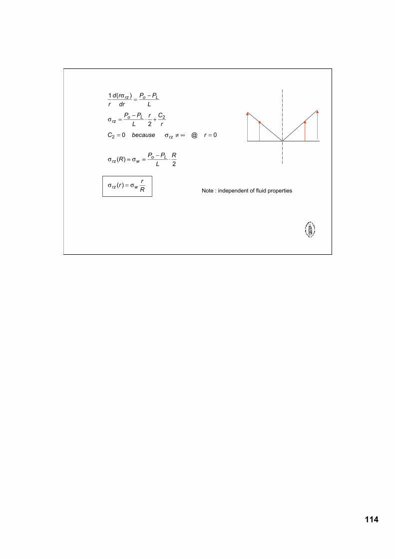
114

1

2

0 0

2

2

2

r

d r

dr

P P

L

P P

L

r C

r

C because r

RP P

L

R

rr

R

rz o L

rzo L

rz

rz wo L

rz w

( )

@

( )

( )

!

!

!

! !

! !

="

="

# +

= $ % =

= ="

#

=

Note : independent of fluid properties

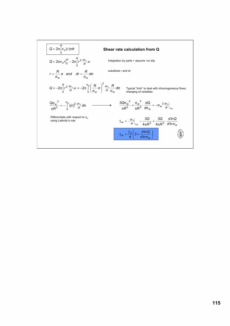
115

( )

Q v r rdr

Q v r r

rR

and drRd

Q rR R

d

Q

Rd

z

R

z

R dv

drdr

R

w w

dv

drdr

R

w

dv

drw

w dv

dr

z

z zw

zw

= !

= " !

= =

= " ! = "#$%

&'(!

= " !

2

2 2

2 2

0

0

2

0

2

0

2

0

3

3

2

0

)

) )

**

**

) )*

**

*

*

)* *

*

*

( )

3

3

4

3

4

43

2

3

3

3

2

3 3

Q

R R

dQ

d

Q

R

Q

R

d Q

d

d Q

d

w w

w

wdv

dr

wdv

drw

wa

w

z

w

z

w

!

"

!

" !!

#" " !

##

!

!

!

+ $ = %

= + $

= +&'(

)*+

% =!ln

ln

!! ln

ln

Integration by parts + assume :no slip

substitute r and dr

Differentiate with respect to σwusing Leibnitz’s rule

Typical “trick” to deal with inhomogeneous flows:changing of variables

Shear rate calculation from Q

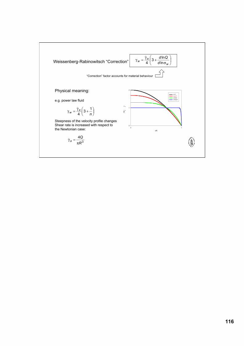
116

r/R

0 1

v

z

/ <v

z

>

0

1

2

n=1

n=0.7

n=0.3

n=0.01

!!

"wa

w

d Q

d= +

#$%

&'(

! ln

ln43Weissenberg-Rabinowitsch “Correction”

“Correction” factor accounts for material behaviour

Physical meaning:

e.g. power law fluid

Steepness of the velocity profile changesShear rate is increased with respect to the Newtonian case:

!!

w

a

n= +

"#$

%&'

!

43

1

!!"

a

Q

R=4

3

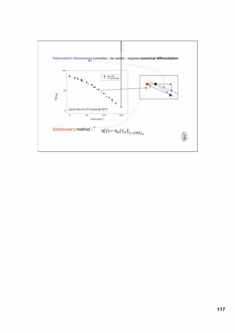
117

typical data of a PP sample @ 230°C

shear rate [s-1

]

10 100 1000 10000

!, !

a

[Pa

.s]

10

100

1000

Raw data

"corrected data"

Rabinowitsch Weissenberg correction : be careful - requires numerical differentiation

Schümmer’s method : ! " ! "" "

( ! ) ( ! )! . !

==a a

a0 83

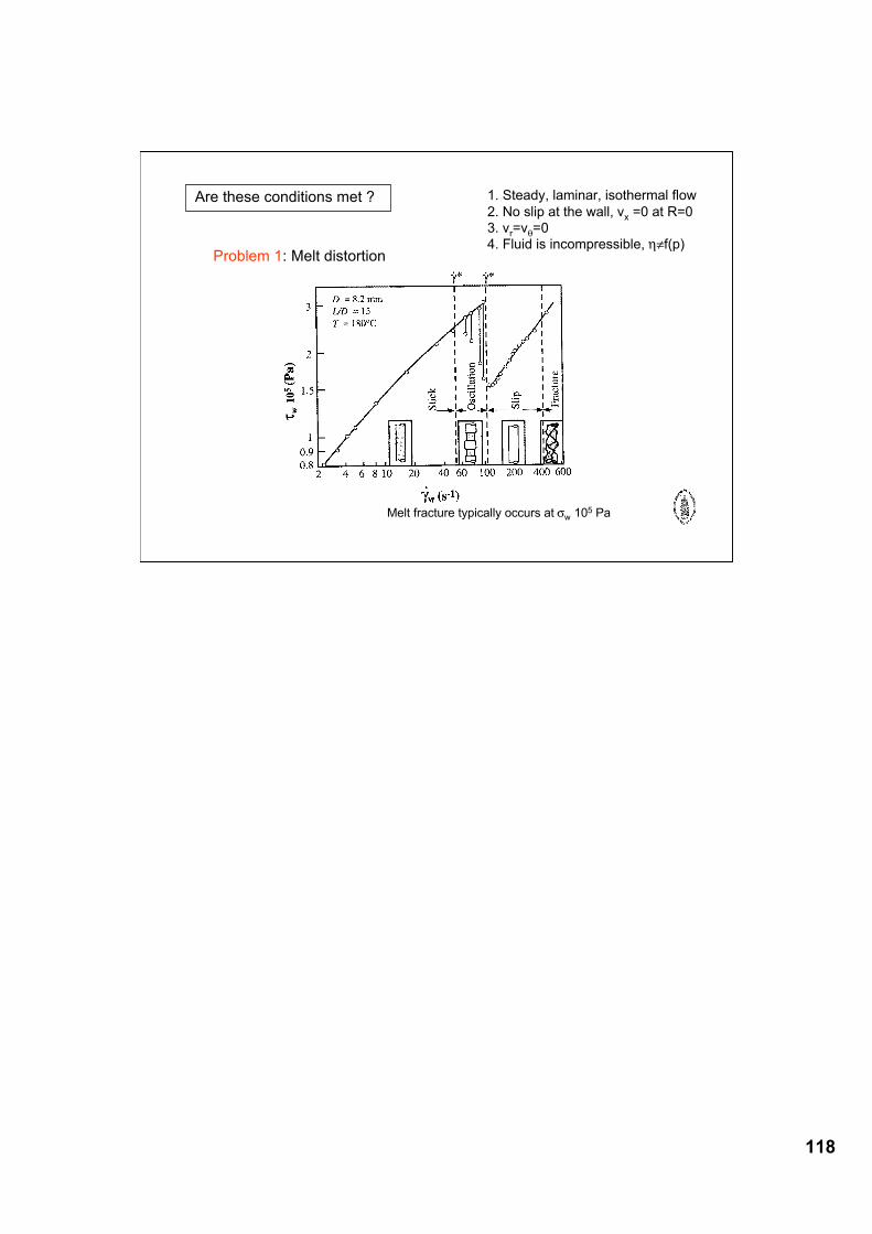
118

Are these conditions met ? 1. Steady, laminar, isothermal flow2. No slip at the wall, vx =0 at R=03. vr=vθ=04. Fluid is incompressible, η≠f(p)

Problem 1: Melt distortion

Melt fracture typically occurs at σw 105 Pa

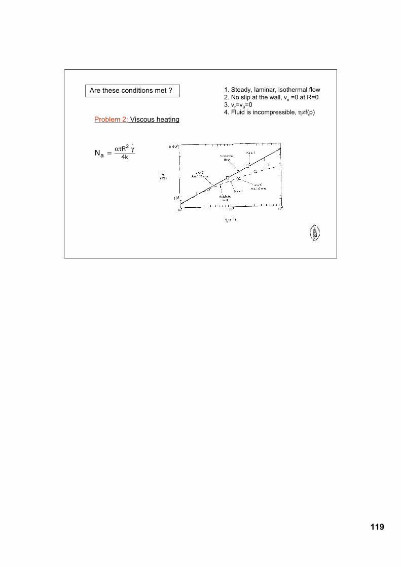
119

Are these conditions met ? 1. Steady, laminar, isothermal flow2. No slip at the wall, vx =0 at R=03. vr=vθ=04. Fluid is incompressible, η≠f(p)

Problem 2: Viscous heating

Na

R

k=

!" #2

4

.

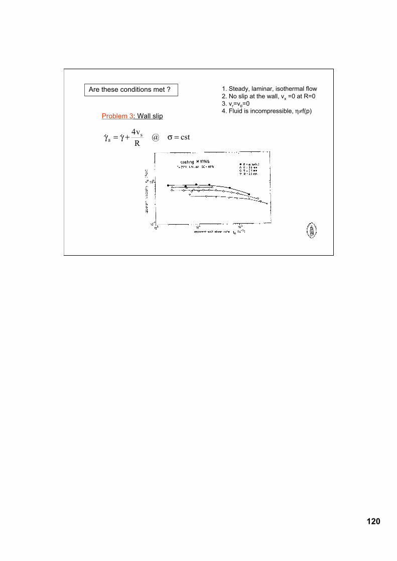
120

Are these conditions met ? 1. Steady, laminar, isothermal flow2. No slip at the wall, vx =0 at R=03. vr=vθ=04. Fluid is incompressible, η≠f(p)

Problem 3: Wall slip

cst@R

v4 sa =!+"=" !!

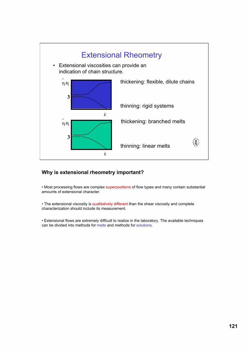
121

• Extensional viscosities can provide anindication of chain structure.

ε̇

η η⁄

3

thinning: rigid systems

ε̇

η η⁄

3

thickening: branched melts

thinning: linear melts

thickening: flexible, dilute chains

Extensional Rheometry

Why is extensional rheometry important?

• Most processing flows are complex superpositions of flow types and many contain substantialamounts of extensional character.

• The extensional viscosity is qualitatively different than the shear viscosity and completecharacterization should include its measurement.

• Extensional flows are extremely difficult to realize in the laboratory. The available techniquescan be divided into methods for melts and methods for solutions.

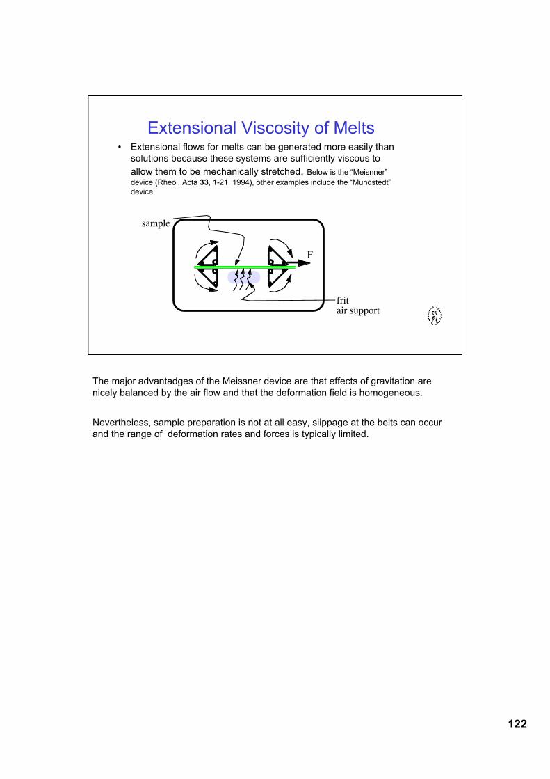
122

Extensional Viscosity of Melts• Extensional flows for melts can be generated more easily than

solutions because these systems are sufficiently viscous toallow them to be mechanically stretched. Below is the “Meisnner”device (Rheol. Acta 33, 1-21, 1994), other examples include the “Mundstedt”device.

F

frit air support

sample

The major advantadges of the Meissner device are that effects of gravitation arenicely balanced by the air flow and that the deformation field is homogeneous.

Nevertheless, sample preparation is not at all easy, slippage at the belts can occurand the range of deformation rates and forces is typically limited.

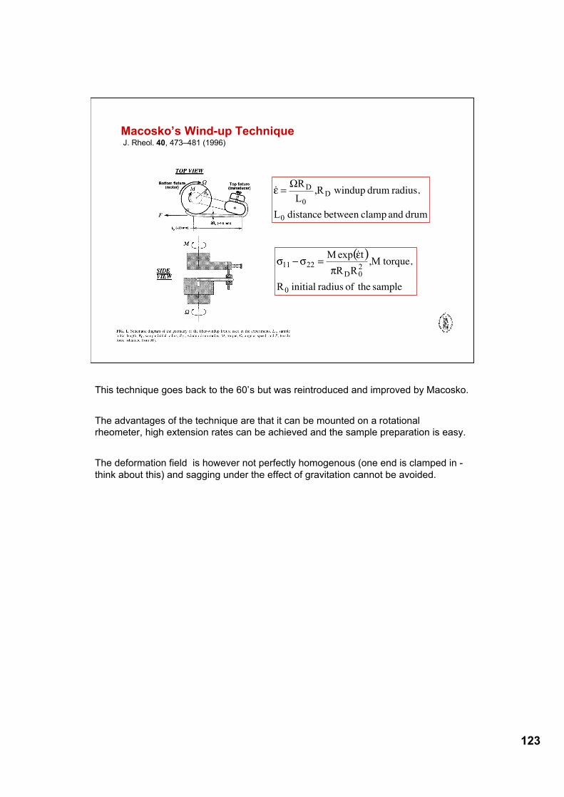
123

Macosko’s Wind-up Technique J. Rheol. 40, 473–481 (1996)

drum and clampbetween distance

radius, drum windup

0

D0

D

L

R,L

R!="!

( )

sample theof radius initial

torque,

0

20D

2211

R

M,RR

texpM

!

"=#$#

!

This technique goes back to the 60’s but was reintroduced and improved by Macosko.

The advantages of the technique are that it can be mounted on a rotationalrheometer, high extension rates can be achieved and the sample preparation is easy.

The deformation field is however not perfectly homogenous (one end is clamped in -think about this) and sagging under the effect of gravitation cannot be avoided.

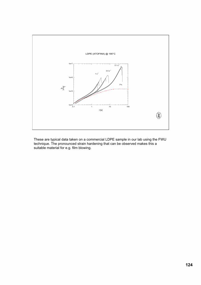
124

3*!afschuiving

t [s]

0.1 1 10 100

!

E

[Pa.s]

1e+4

1e+5

1e+6

1e+7

3*!

1 s-1

0.5 s-1

0.1 s-1

LDPE (ATOFINA) @ 190°C

These are typical data taken on a commercial LDPE sample in our lab using the FWUtechnique. The pronounced strain hardening that can be observed makes this asuitable material for e.g. film blowing.

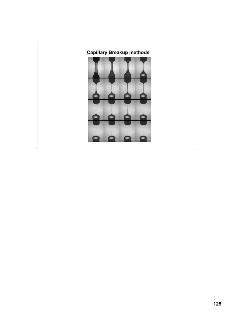
125

Capillary Breakup methods

126

Current Research Topics

- Linking rheology and structure:Rheo-optics, Rheo-scattering,...

- Rheology of complex fluid interfaces

- Microrheological methods

- Rheology of soft matter composites

- Role of rheology in biological systems

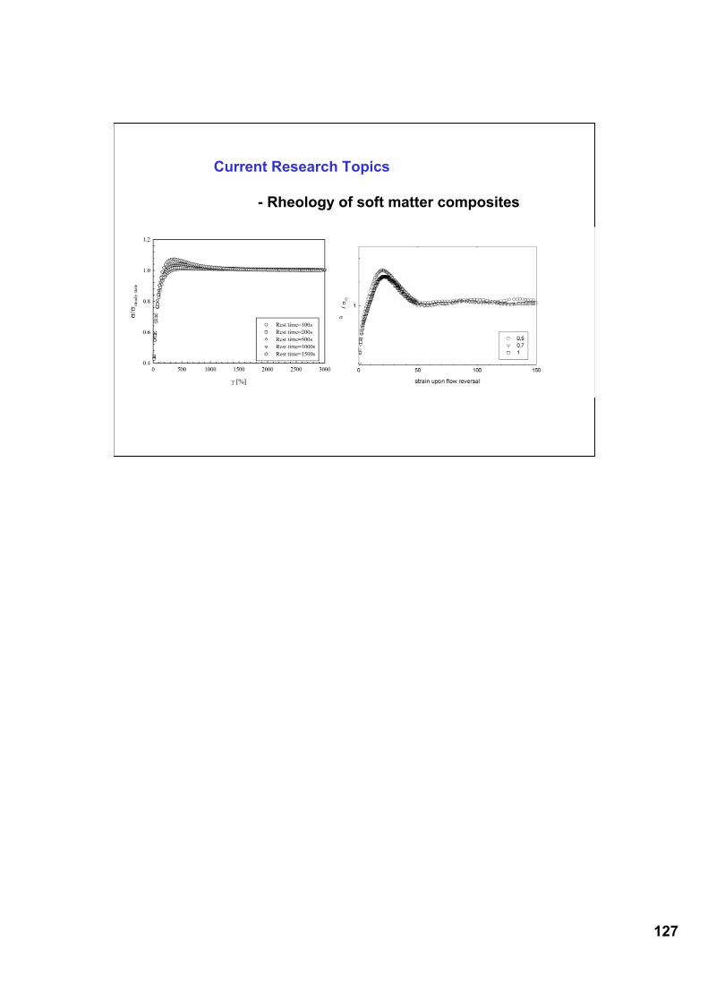
127

Current Research Topics

- Rheology of soft matter composites

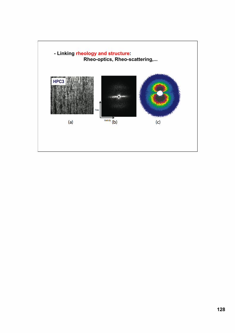
128

- Linking rheology and structure:Rheo-optics, Rheo-scattering,...

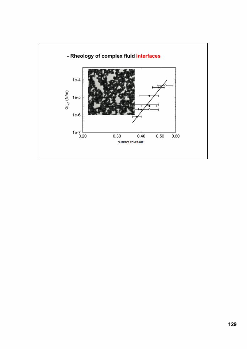
129

- Rheology of complex fluid interfaces

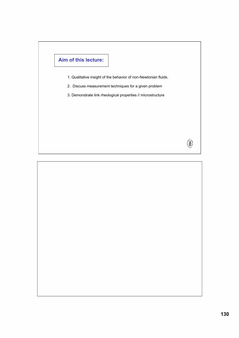
130

Aim of this lecture:

1. Qualitative insight of the behavior of non-Newtonian fluids.

2. Discuss measurement techniques for a given problem

3. Demonstrate link rheological properties // microstructure