RF GUIDELINES 1800 A - cosconor.fr 1800MHz.pdf · RF GUIDELINES 1800 MHz THE ERICSSON GSM SYSTEM R8 ... parameter in the propagation model. General recommendations for …

10/100 56-100/FCP 103 1229/3 Rev A 2000-08-14 1(44)

RF GUIDELINES

1800 MHz

THE ERICSSON GSM SYSTEM R8

Ericsson Radio Systems AB 2000

The contents of this product are subject to revision without notice due tocontinued progress in methodology, design and manufacturing.

Ericsson assumes no legal responsibility for any error or damage resultingfrom usage of this product.

This product is classified as Ericsson Wide Internal

RF GUIDELINES 1800 MHz

2(44) 10/100 56-100/FCP 103 1229/3 Rev A 2000-08-14


10/100 56-100/FCP 103 1229/3 Rev A 2000-08-14 3(44)

Contents

1 Revision history ................................................................. 52 Introduction ........................................................................ 53 Equipment characteristics ................................................ 5

3.1 RBS 2000 .............................................................................................. 6

3.2 RBS 205 ................................................................................................ 9

3.3 Mobile station ...................................................................................... 11

3.4 Antenna near part................................................................................ 12

3.5 Repeaters ............................................................................................ 18

4 Cell coverage.................................................................... 19

4.1 Definitions............................................................................................ 19

4.2 Margins................................................................................................ 20

4.3 Design levels ....................................................................................... 24

4.4 Coverage acceptance test................................................................... 28

5 Cell planning..................................................................... 30

5.1 Wave propagation models for estimation............................................ 30

5.2 Power budget ...................................................................................... 31

5.3 Power balance..................................................................................... 32

5.4 Cell size ............................................................................................... 35

6 References........................................................................ 37

Appendix:1. Curves of Jakes formula, Cumulative normal function

2. Simulated log-normal fading margins

3. Quick reference - Cell planning GSM 1800


4(44) 10/100 56-100/FCP 103 1229/3 Rev A 2000-08-14


10/100 56-100/FCP 103 1229/3 Rev A 2000-08-14 5(44)

1 Revision history

Revision Date Description

A 2000-08-14 First revision, based on RF Guidelines,Ericsson GSM System R7.

URL links updated.

RBS 2206 figures added.

New CDUs added.

Log-normal fading margin (LNFmarg)changed.

Coverage level in percent for a cell changed.

Figure added for rural areas to the Aparameter in the propagation model.

General recommendations for antenna tilting.

Maxite™ figures updated.

References updated and added.

2 IntroductionThis document contains information about site equipment and cell planningpolicy for GSM 1800.

The GSM 1800 system is required to operate in the following frequency band,with a carrier spacing of 200 kHz:

Table 1. Frequency band of GSM 1800.

MS transmit, BTS receive 1710-1785 MHz

Base transmit, MS receive 1805-1880 MHz

3 Equipment characteristicsIn this chapter the equipment characteristics are presented. All valuespresented represent guaranteed values from base station, which are intended tobe used in link budgets for cell planning.

Important note: Some of the equipment mentioned in this document is stillbeing developed. Always check when the equipment you intend to use is


6(44) 10/100 56-100/FCP 103 1229/3 Rev A 2000-08-14

available. Furthermore, the figures for sensitivity and output power maychange. The most recent figures for sensitivity and output power can be foundin ref. 1 and ref. 2, or at:http://gsmrbs.ericsson.se/marketing/FAQ/faq.htm, which is continuouslyupdated.

In the GSM specification (ref. 3), reference sensitivity levels are mentioned.As well the BTSs as MSs must meet some predefined performance values interms of FER, BER and RBER1 defined in the GSM specification. The actualsensitivity level is defined as the input level for which the performance is metand should be less than a specified limit, called the reference sensitivity level.This section contains reference values for different types of BTSconfigurations and MS power classes. At temperatures exceeding 30°C andfor hilly terrain the sensitivity figures can be changed, see ref. 1 and ref. 2.

3.1 RBS 2000RBS 2000 (ref. 4) is the second generation of Ericsson base BTSs for GSM.six different types of RBSs are available: 2101 (2 TRU outdoor cabinet), 2102(6 TRU outdoor cabinet), 2202 (6 TRU indoor cabinet), RBS 2302 (2 TRUmicro BTS), RBS 2401 (2 TRX indoor base station) and RBS 2206 (12 TRUindoor cabinet).

.

For RBS 2101, 2102 and 2202, functional units as for example combiners areincluded in a Combining and Distribution Unit (CDU). There are threedifferent CDU types, A, C+ and D, all with different characteristics. Whenselecting CDU type, three different alternatives exist, the antennas referred toare cross-polarized:

• Maximum Range (CDU-A). It is designed to maximise the output power.With this alternative up to 2 TRUs can be connected to one antenna in acell but it is configurable for up to 6 TRUs.

• Standard (CDU-C+). It contains a hybrid combiner, which allows 4 TRUsto be connected to one antenna in a cell but is configurable for up to 12TRUs.

• High Capacity (CDU-D). It contains a filter combiner, which makes itpossible to connect up to 12 TRUs to one antenna in a cell. Using CDU-D,it is not possible to perform synthesizer frequency hopping, only baseband hopping.

There is another alternative, Smart Range, which allows a CDU-A and aCDU-C+ to be combined in the same cell. This solution combines highcoverage with high capacity, up to 6 TRUs per cell can be connected.

1 FER = Frame Erasure Ratio; BER = Bit Error Ratio; RBER = Residual Bit Error Ratio


10/100 56-100/FCP 103 1229/3 Rev A 2000-08-14 7(44)

For RBS 2206 there exist two different types of CDUs, F and G, both withdifferent characteristics and the possibility to be used together with TMA. Thenew CDUs makes it possible to support 3x4 configurations in one cabinet. Theantennas referred to are cross-polarized:

• CDU-F. It contains a filter combiner, which makes it possible to connectup to 12 TRUs to one antenna in a cell. It is not possible to performsynthesizer frequency hopping, only base band hopping.

• CDU-G. With CDU-G the RBS 2206 can be configured in two modes:capacity mode or coverage mode. In capacity mode up to 12 TRUs can beconnected to 2 antennas in a cell. It supports both synthesizer hopping andbase band hopping.

Software Power Boost can be used to improve the downlink output power forRBS 2000 and thus achieve better coverage. A prerequisite is that CDU-A orCDU-G is used and that each cell is equipped with 2 TRUs per cell. TX-diversity is then used in order to obtain a downlink diversity gain of 3 dB,which should be added to the link budget.

Software Power Boost gain 3 dB

The RBS 2206 (ref. 8) is a macro base station supporting up to 12 TRUs percabinet, which can be configured as one, two or three sector cellconfiguration.

For more information concerning RBS configurations for macrocells, seeref. 5.

The RBS 2302 (ref. 6) is a micro base station. 3 RBS 2302s can be connectedin order to build up to 6 TRUs per cell (note: BTS 7.1 required). SoftwarePower Boost can also be used together with RBS 2302.

The RBS 2401 (ref. 7) is the first dedicated pico radio base station, designedfor indoor applications. It is equipped with 2 TRXs.

The output power, sensitivity and minimum carrier separation of theRBS 2000 series are listed in Table 2.


8(44) 10/100 56-100/FCP 103 1229/3 Rev A 2000-08-14

Table 2. Output power, sensitivity and minimum carrier separation ofRBS 2000.

CDU/RBS Output power[dBm]

Sensitivity[dBm]

Minimum carrierseparation [kHz]

A 43.5 -1101 4003

C2 40 -1101 4003

C+ 40 -1101 4003

D 41 -1101 1000

F 42.0 -1101 800

G 42.0/45.54 -1101 400

RBS 2302 33 -106 400

RBS 2401 22 -100 400

1 With TMA the sensitivity is –111.5 dBm. This sensitivity figure applies forantenna feeders with up to 4 dB loss. If the loss between the TMA and theBTS exceeds 4 dB the sensitivity is decreased, as described in section 3.4.3.

2CDU-C is today replaced by CDU-C+.

3The CDU can from a radio performance perspective handle 200 kHz carrierseparation, but bursts may then be lost due to low C/A. From a system point ofview the consequences of going below 400 kHz are not fully investigated.Problems with for example standing wave alarms may occur. Thus it isrecommended to keep 400 kHz carrier separation.

4 Output power is 42.0 dBm if hybrid combiner is used in the dTRU.

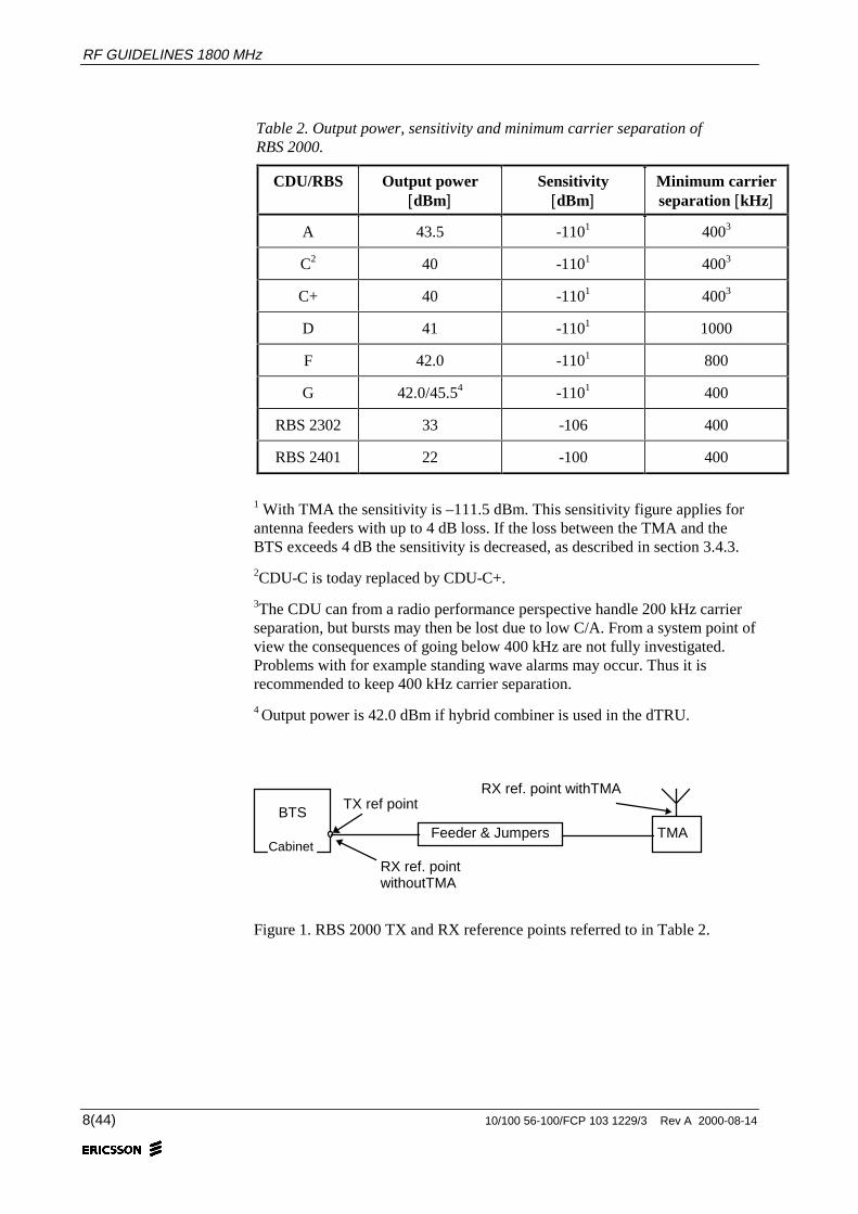
TMAFeeder & JumpersCabinet

BTSTX ref point

RX ref. point withTMA

RX ref. pointwithoutTMA

Figure 1. RBS 2000 TX and RX reference points referred to in Table 2.


10/100 56-100/FCP 103 1229/3 Rev A 2000-08-14 9(44)

3.2 RBS 205RBS 205 (ref. 9) belongs to the first generation of Ericsson base stations forGSM. Each cabinet can take 4 Transceivers (TRX), and the cabinets must beplaced indoors. The RBS 200 is designed for different types of combiners:filter combiners and hybrid combiners.

With filter combiners 1 to 8 transmitters can be connected to the sameantenna. In order to use 9 to 16 transmitters in a cell, two filter combiners andtwo transmitting antennas must be used. Using filter combiners it is notpossible to perform synthesizer frequency hopping, only base band hopping.

With one hybrid combiner 2 transmitters can be connected to one antenna andusing three combiners 4 transmitters can be connected to the same antenna.Hybrid combiners allow both base band hopping and synthesizer hopping.

Table 3 shows the output power, sensitivity and minimum carrier separationfor the different configurations.

Table 3. Output power, sensitivity and minimum carrier separation of RBS205.

Combiner type Output power[dBm]

Sensitivitywithout TMA

[dBm]


Filter (1-8 TX) 40 -106 1200

Hybrid (2 TX) 39.5 -106 4001

3 x Hybrid (3-4 TX) 36 -106 4001

1The combiner can from a radio performance perspective handle 200 kHzcarrier separation, but bursts may then be lost due to low C/A. From a systempoint of view the consequences of going below 400 kHz are not fullyinvestigated. Problems with for example standing wave alarms may occur.Thus it is recommended to keep 400 kHz carrier separation.


10(44) 10/100 56-100/FCP 103 1229/3 Rev A 2000-08-14

TMAFeeder & JumpersCabinet

BTSTX ref point

RX ref. point withTMA

RX ref. pointwithoutTMA

Figure 2 RBS 205 TX and RX reference points referred to in Table 3.

3.2.1 MaxiteTo provide a possibility of extending the limited coverage area of RBS 2302,Maxite (ref. 10) has been developed. Maxite consists of an RBS 2302together with an Active Antenna Unit (AAU) and a Power Battery Cabinet(PBC). The AAU contains a set of distributed power amplifiers for thetransmitted signals, a low noise amplifier for the received signals and anintegrated patch antenna. Apart from extending the coverage of the RBS 2302similar to a macrocell, it also provides the possibility to use thinner antennafeeders.

There is one type of AAU with power capabilities of 500W EIRP. Itcharacteristics is described in Table 4. The values for output power andsensitivity are valid for a feeder loss of maximum 10 dB.


10/100 56-100/FCP 103 1229/3 Rev A 2000-08-14 11(44)

Table 4. Equipment characteristics of Maxite.

MaxiteProduct

Antenna Diversitygain

Slant loss Outputpower

Sensitivity

Minimumcarrier

separation

Maxite 500W

17.5 dBi 3.5 dB 1 dB 40 dBm -111 dBm 400 kHz

RBS2302

Feeder & jumpersTX and RX ref.

AAU

Figure 3. Maxite TX and RX reference points. Both TX and RX referencepoints are defined at the antenna inside the AAU.

3.3 Mobile stationThere are three MS power classes described in the GSM 1800 Specification(ref. 3) however only MSs of class 1 and 2 are likely to be used. Typicalfigures for maximum output power and sensitivity are shown in Table 5. Thefigures are specified at the MS antenna connector.

Table 5. MS power classes.

MS power class Output power [dBm] Sensitivity [dBm]

1 30 -104

2 24 -104

According to the GSM Specification, the sensitivity is –102 dBm for GSM1800 MSs. However experiences from leading mobile manufacturers showthat the sensitivity is 2 – 4 dB better and therefore this value is set to -104dBm dBm, see e.g. ref. 11.

No loss or antenna gain should be used for the MSs.

MS antenna gain: 0 dBi


12(44) 10/100 56-100/FCP 103 1229/3 Rev A 2000-08-14

3.4 Antenna near partMore information about the equipment mentioned in this section and thefollowing can be found at the Ericsson intranet:http://gsmrbs.ericsson.se/gsmsystems/solutions/rbs_site_solutions/antenna_systems/

3.4.1 Base station feeders and jumpersWhen calculating the power budget, the feeder loss must be taken intoaccount. The most commonly used feeder type is 7/8”. In Table 6, the lossesfor the most common macrocell feeder types are listed (ref. 12).

Table 6. Attenuation in some feeder types at 1800 MHz.

Feeder type Attenuation [dB/100m]

LCF 1/2” 10.5

LCF 7/8” 6.5

LCF 1-1/4” 5.3

LCF 1-5/8” 4.2

Apart from the feeder loss, additional loss will arise in jumpers andconnectors. Typical values are 0.5 dB for every jumper and 0.1 dB for everyconnector.

3.4.2 External filtersDuplex filters make it possible to use the same antenna for transmission andreception. When an external duplex filter is used there will be an additionalloss in both uplink and downlink.

Apart from external duplexers, some TMAs contain duplex filters, see section3.4.3. Duplex filters can be used with RBS 205; RBS 2000 contains internalfilters.

Table 7. Duplex attenuation values

Devise Typical loss [dB]

External duplex filter 0.5

Diplex filters make it possible to use the same feeders for GSM 900 asGSM 1800 in a dual band site. They are needed in order to differentiate thetwo frequency bands.


10/100 56-100/FCP 103 1229/3 Rev A 2000-08-14 13(44)

Table 8. Diplex attenuation values

Devise Typical loss [dB]

External diplex filter 0.3

Data sheets for filters can be found at: http://rsaweb.ericsson.se/market/filter-shop/brochures/

3.4.3 Tower Mounted AmplifiersIn order to improve the sensitivity on the uplink a Tower Mounted Amplifier(TMA) can be used. The purpose of the TMA is to amplify the received signalbefore it is further attenuated in the antenna feeder. There are two types ofTMA with different number of duplex filters, see Table 9.

Table 9. TMA products for RBS 2000.

TMA products # Duplexers TMA downlink loss [dB]

RBS 2000 TMA 1800 Simplex 0 0

RBS 2000 TMA 1800 Duplex 1 0.3

RBS 2000 TMA 1800 Dual Duplex 2 0.3

With a TMA the receiver sensitivity will not be affected by the loss in thefeeder as long as it does not exceed 4 dB. When the loss exceeds 4 dB thesensitivity decreases according to Table 10 (ref. 13). For example thesensitivity of CDU-A with a feeder loss of 8 dB between the RBS and theTMA would become –111.5 + 1.5 = -110 dBm at the TMA connector. Formore information about how to use TMA, see ref. 14.

Table 10. Sensitivity deterioration when the loss between the TMA and theBTS exceeds 4 dB.

Loss [dB] Sensitivity deterioration [dB]

≤ 4 0

6 0.5

8 1.5

10 2.5


14(44) 10/100 56-100/FCP 103 1229/3 Rev A 2000-08-14

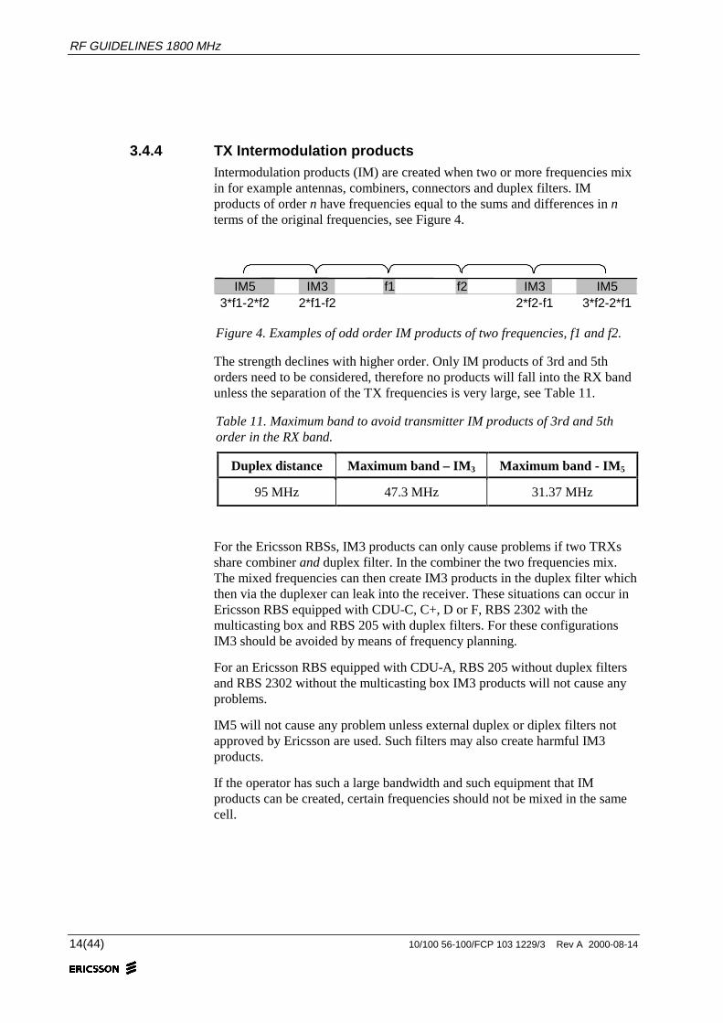
3.4.4 TX Intermodulation productsIntermodulation products (IM) are created when two or more frequencies mixin for example antennas, combiners, connectors and duplex filters. IMproducts of order n have frequencies equal to the sums and differences in nterms of the original frequencies, see Figure 4.

IM5 IM3 f1 f2 IM3 IM53*f1-2*f2 2*f1-f2 2*f2-f1 3*f2-2*f1

Figure 4. Examples of odd order IM products of two frequencies, f1 and f2.

The strength declines with higher order. Only IM products of 3rd and 5thorders need to be considered, therefore no products will fall into the RX bandunless the separation of the TX frequencies is very large, see Table 11.

Table 11. Maximum band to avoid transmitter IM products of 3rd and 5thorder in the RX band.

Duplex distance Maximum band – IM 3 Maximum band - IM 5

95 MHz 47.3 MHz 31.37 MHz

For the Ericsson RBSs, IM3 products can only cause problems if two TRXsshare combiner and duplex filter. In the combiner the two frequencies mix.The mixed frequencies can then create IM3 products in the duplex filter whichthen via the duplexer can leak into the receiver. These situations can occur inEricsson RBS equipped with CDU-C, C+, D or F, RBS 2302 with themulticasting box and RBS 205 with duplex filters. For these configurationsIM3 should be avoided by means of frequency planning.

For an Ericsson RBS equipped with CDU-A, RBS 205 without duplex filtersand RBS 2302 without the multicasting box IM3 products will not cause anyproblems.

IM5 will not cause any problem unless external duplex or diplex filters notapproved by Ericsson are used. Such filters may also create harmful IM3products.

If the operator has such a large bandwidth and such equipment that IMproducts can be created, certain frequencies should not be mixed in the samecell.


10/100 56-100/FCP 103 1229/3 Rev A 2000-08-14 15(44)

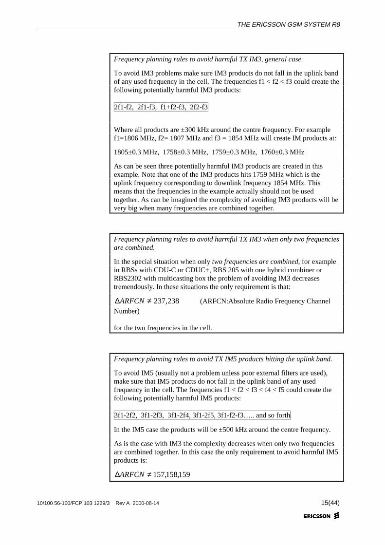
Frequency planning rules to avoid harmful TX IM3, general case.

To avoid IM3 problems make sure IM3 products do not fall in the uplink bandof any used frequency in the cell. The frequencies f1 < f2 < f3 could create thefollowing potentially harmful IM3 products:

2f1-f2, 2f1-f3, f1+f2-f3, 2f2-f3

Where all products are ±300 kHz around the centre frequency. For examplef1=1806 MHz, f2= 1807 MHz and f3 = 1854 MHz will create IM products at:

1805±0.3 MHz, 1758±0.3 MHz, 1759±0.3 MHz, 1760±0.3 MHz

As can be seen three potentially harmful IM3 products are created in thisexample. Note that one of the IM3 products hits 1759 MHz which is theuplink frequency corresponding to downlink frequency 1854 MHz. Thismeans that the frequencies in the example actually should not be usedtogether. As can be imagined the complexity of avoiding IM3 products will bevery big when many frequencies are combined together.

Frequency planning rules to avoid harmful TX IM3 when only two frequenciesare combined.

In the special situation when only two frequencies are combined, for examplein RBSs with CDU-C or CDUC+, RBS 205 with one hybrid combiner orRBS2302 with multicasting box the problem of avoiding IM3 decreasestremendously. In these situations the only requirement is that:

238,237≠∆ARFCN (ARFCN:Absolute Radio Frequency ChannelNumber)

for the two frequencies in the cell.

Frequency planning rules to avoid TX IM5 products hitting the uplink band.

To avoid IM5 (usually not a problem unless poor external filters are used),make sure that IM5 products do not fall in the uplink band of any usedfrequency in the cell. The frequencies f1 < f2 < f3 < f4 < f5 could create thefollowing potentially harmful IM5 products:

3f1-2f2, 3f1-2f3, 3f1-2f4, 3f1-2f5, 3f1-f2-f3….. and so forth

In the IM5 case the products will be ±500 kHz around the centre frequency.

As is the case with IM3 the complexity decreases when only two frequenciesare combined together. In this case the only requirement to avoid harmful IM5products is:

159,158,157≠∆ARFCN


16(44) 10/100 56-100/FCP 103 1229/3 Rev A 2000-08-14

for the two frequencies in the cell.

3.4.5 DiversityOne way of reducing the influence of multipath fading in the uplink is to useantenna diversity. In the Ericsson GSM system this means that the signalsfrom two RX branches are decoded and the most probable bit values arechosen on a bit per bit basis. The result of the method is equivalent tomaximum likelihood estimation. The antenna diversity gain will depend on thecorrelation between the fading of two antenna signals as well as the efficiencyin power reception of the two separate antennas. There are two different typesof antenna diversity: space diversity and polarization diversity.

Space diversity means that two RX antennas positioned at a certain minimumdistance from each other are used. Typically, space diversity improves theuplink by 3.5 dB. The separation required to obtain sufficient space diversitygain for various configurations and antennas is described in ref. 15 (alsoavailable at the Ericsson intranet:http://gsmrbs.ericsson.se/RBS_Site_Solutions_Antenna_Systems/RBS_Antennas/Intranet/ant_mounting_guides.htm).

Polarization diversity offers relief by allowing two space diversity antennasseparated by several meters to be replaced by one dual polarized antenna. Thisantenna has normal size but contains two differently polarized antenna arrays.

It has been shown (see ref. 16) that due to different propagation characteristicsthe propagation loss for the horizontally polarized component is larger thanfor the vertical component. This consequence is that an extra “slant loss”margin of 1 dB must be added to the normal path loss when ±45°polarizedantennas are used. However, a dual polarized antenna offers very lowcorrelation in critical environments such as indoor and in-car. In thesesituations the diversity gain of polarization is about 1 dB better than spacediversity. This is just enough to compensate for the slant loss. For simplicitythe uplink slant loss is in this document included in the diversity gain. Thismeans that for space as well as polarization diversity the uplink gain is 3.5 dB,and that no slant loss should be added to the uplink.

Space and polarization diversity gain 3.5 dB

In order to compensate for the downlink slant loss, 1 dB must be added to thedownlink propagation loss.


10/100 56-100/FCP 103 1229/3 Rev A 2000-08-14 17(44)

Slant (±45°) polarization downlink loss 1 dB

3.4.6 AntennasThere are a large number of antenna types available. Antennas for macrocelluse can have various widths and shapes of the radiation pattern, giving a largespread in gain. The vertical lobe can be down tilted, the antennas can be dualpolarized in some way and they can be more or less broad banded.

The standard antenna for a three-sector site has a horizontal beam width of65°. This means that the gain at 32.5° is 3 dB less than the maximum gain. At60° it is suppressed typically 10 dB. The gain of a macrocell antenna istypically 15-18 dBi. Broader antennas with 90° and 105° horizontal beamwidths are alternatives. However, the difference in shape of the coverage areais small but the gain is slightly lower for a certain antenna length. Omniantennas for 1800 MHz have a typical gain of 8-11 dBi.

All antennas used shall comply with the basic specifications, which can befound on the Ericsson intranet at:http://gsmrbs.ericsson.se/RBS_Site_Solutions_Antenna_Systems/RBS_Antennas/Intranet/ant_basicspecs.htm

3.4.7 Antenna isolationThe isolation between two antennas is defined as the attenuation from theconnector of one antenna to the connector of the other antenna.

To avoid unwanted signals into the receiver, the isolation should be at least 30dB between the transmitting and receiving antenna and between twotransmitting antennas.

To obtain the required isolation values, the antennas must be positioned at acertain minimum distance from each other. The distance depends on theantenna types and on the configuration, see ref. 15 (also available on theEricsson intranet:http://gsmrbs.ericsson.se/RBS_Site_Solutions_Antenna_Systems/RBS_Antennas/Intranet/ant_mounting_guides.htm)

3.4.8 Antenna tiltingAntenna tilting means that the main vertical beam of the antenna is directedtowards a point below the horizon, so called downtilt. Tilting is used incellular systems basically for two reasons: to improve coverage at small cellsites with high antenna positions and to improve co-channel interference.There are two different kinds of tilt: electrical and mechanical tilt.


18(44) 10/100 56-100/FCP 103 1229/3 Rev A 2000-08-14

Electrical tilt means an in-built tilt that lowers the vertical beam in allhorizontal directions. The tilting angle is normally fixed. When usingmechanical tilt, the antenna is mounted with adjustable brackets in a way thatthe antenna can be adjusted on site. Mechanical tilt is only used on directionalantennas. It is also possible to combine these two tilt methods.

There are two rules of thumb regarding antenna tilting, see ref. 17:

• If a maximum reduction in co-channel interference is desired, the firstnotch in the vertical antenna pattern should be aimed towards the areawhere a reduction of interference is desired. This may however result inan undesired decrease in signal strength at the cell border.

• If a minimum coverage reduction is desired, then the antenna may be tilteduntil the vertical beam points towards the cell border. About 1° additionaltilt may be used without any significant decrease in signal strength at thecell border. Thus tilting the antenna towards the cell border is a safe wayof increasing the carrier to interference ratio (C/I), without jeopardisingthe coverage.

In ref. 18 there are some general recommendations for antenna tilting:

• There is no point in tilting an antenna less than the angle which gives a3dB loss at the horizon. This corresponds to around 7° tilt for a 15 dBiantenna, and around 3.5° tilt for an 18 dBi antenna. A smaller tilt gives alimited impact and is hardly worth the effort.

• Study the antenna diagram carefully before selecting the tilt-angle. Mostof the tilting effect happens between the angle corresponds to the 3 dBpoint towards the horizon, and the angle that corresponds to tilting thefirst null towards the horizon. For example 8° tilt gives far more thantwice the effect compared to 4°.

• Avoid down tilting more than the angle that corresponds to having the firstnull towards the horizon. Further down tilting can be done in extremecases, but if there is a need for further reduction of interference or cellsize, a reduction of output power, or possibly lowering of the antennaheight, should also be considered. Very large down tilts (beyond the firstnull towards the horizon) should be carefully verified since the effect ofsuch large tilts is difficult to predict.

• Verify all the effects after having performed a down tilt of more than 8°(15 dBi antennas) or 4° (18 dBi antennas). Remember that it is just asimportant to check the coverage and quality in the down tilted cell, as thearea where the down tilt is expected to reduce interference. Even if oneproblem is solved, a new problem might have occurred.

3.5 RepeatersA repeater can cover areas that otherwise would have been blocked byobstacles. Fields of application are roads in hilly terrain, tunnels or other


10/100 56-100/FCP 103 1229/3 Rev A 2000-08-14 19(44)

obstructed low capacity areas. Repeaters can also be used for indoorapplications. The signal is typically amplified by 50-80 dB. However, asystematic use of repeaters in order to save base stations have not shown outto be effective. For more information about how to cell plan with repeaters,see ref. 19 and ref. 20.

Some repeater types can not be used together with dynamic BTS powerregulation. They produce a constant output power at incoming signalsexceeding a threshold and no power at all for signals below that threshold.The connection is lost when the down regulation has brought the signal belowthe threshold. With constant gain in the repeater instead, the down regulationstops automatically when quality suffers.

4 Cell coverageSection 3 presents the sensitivity level for both the MS and the BTS.However, when planning a system it is not sufficient to use this sensitivitylevel as a planning criterion. Various margins have to be added in order toobtain the desired coverage. In this chapter these margins are discussed andthe planning criteria to use in different types of environments are presented.Furthermore the principles of how to perform coverage acceptance tests aredescribed.

4.1 DefinitionsRequired signal strength

To the sensitivity level of an MS, margins have to be added to compensate forRayleigh fading, interference and body loss. The obtained signal strength iswhat is required to perform a phone call in a real-life situation and will bereferred to as SSreq. SSreq is independent of the environment.

SSreq = MSsens + RFmarg + IFmarg + BL (1)

where

MSsens = MS sensitivity, Section 3.3.RFmarg = Rayleigh fading margin, Section 4.2.1.IFmarg = Interference margin, Section 4.2.3.BL = Body loss, Section 4.2.4.

Design level

Extra margins have to be added to SSreq to handle the log-normal fading aswell as different types of penetration losses. These margins depend on theenvironment and on the desired area coverage. The obtained signal strength iswhat should be used when planning the system and it will be referred to as thedesign level, SSdesign. This signal strength is the value that should be obtainedon the cell border when planning with prediction tools like EET/TCP.


20(44) 10/100 56-100/FCP 103 1229/3 Rev A 2000-08-14

The design level can be calculated from:

SSdesign = SSreq + LNFmarg(o) MS outdoor (2)

SSdesign = SSreq + LNFmarg(o) + CPL MS in-car (3)

SSdesign = SSreq + LNFmarg(o+i) + BPLmean MS indoor (4)

where

LNFmarg(o) = Outdoor log-normal fading margin, Section 4.2.2LNFmarg(o+i) = Outdoor + indoor log-normal fading margin, Section 4.2.2CPL = Car penetration loss, Section 4.2.5BPLmean = Mean building penetration loss, Section 4.3.2

4.2 Margins

4.2.1 Rayleigh fadingRayleigh fading is due to multipath interference and occurs especially in urbanenvironments where there is high probability of blocked sight betweentransmitter and receiver. The distance between two adjacent fading dips isapproximately λ/2.

The required sensitivity performance of GSM in terms of FER, BER or RBERis specified for each type of channel and at different fading models (calledchannel models). The channel models reflect different types of propagationenvironment and different MS speeds. The sensitivity is measured undersimulated Rayleigh fading conditions for all the different channel models andthe sensitivity is defined as the level where the required quality performance isachieved. In a noise limited environment the sensitivity is the one listed inChapter 1. This would mean that Rayleigh fading is already taken intoconsideration in the sensitivity definition.

However, the GSM specification allows worse quality for slow MSs (3 km/h)than for fast moving MSs. The sensitivity performance at fading conditionscorresponding to an MS speed of 50 km/h in an urban environment (calledTU502), is in accordance with good speech quality, while the sensitivityperformance for slow MSs at TU32 does not correspond to acceptable speechquality.

In order to obtain good speech quality even for slow mobiles, an extra margin,RFmarg, is recommended when planning. From experience, 3 dB margin seemsadequate. In a frequency hopping system the Rayleigh fading dips are levelledout and there should be no need for a Rayleigh fading margin. But since aBroadcast Control Channel (BCCH) never hops, the Rayleigh fading margin isrecommended in cell coverage estimations, regardless of using frequency

2 TU50 = Typical Urban 50 km/h, TU3 = Typical Urban 3 km/h


10/100 56-100/FCP 103 1229/3 Rev A 2000-08-14 21(44)

hopping or not. Also antenna diversity reduces the effect of Rayleigh fadingbut in a different way than frequency hopping. Therefore, diversity gain is stillrelevant in frequency hopping systems. (For simplicity the diversity gainfigure is considered independent of frequency hopping and MS speeddistribution).

Rayleigh fading margin (RFmarg) = 3 dB

4.2.2 Log-normal fadingThe signal strength value computed by wave propagation algorithms can beconsidered as a mean value of the signal strength in a small area with a sizedetermined by the resolution and accuracy of the model. Assumed that the fastfading is removed, the local mean value of the signal strength fluctuates in away not considered in the prediction algorithm. This deviation of the localmean in dB compared to the predicted mean has nearly a normal distribution.Therefore this variation is called log-normal fading.

The received signal strength is a random process and it is only possible toestimate the probability that the received signal strength exceeds a certainthreshold. In the result from a prediction in for example EET or TCP, 50% ofthe locations (for example at the cell borders) can be considered to have asignal strength that exceeds the predicted value. In order to plan for more than50% probability of signal strength above the threshold, a log-normal fadingmargin, LNFmarg, is added to the threshold during the design process.

Jakes’ formulas

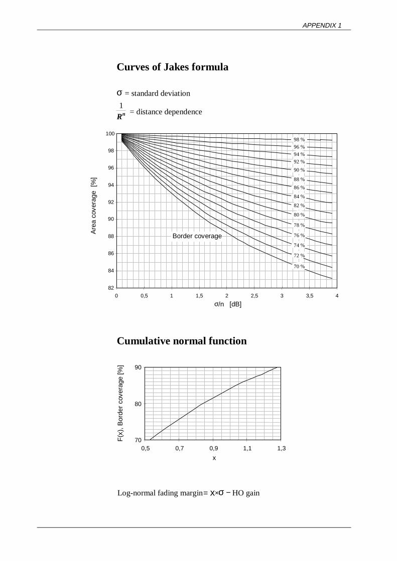
A common way to calculate LNFmarg is to use Jakes’ formulas, ref. 21. InJakes’ formulas a simple radial path loss dependence (1/rn) is assumed inorder to calculate the percentage of area within an omni-cell with signalstrength exceeding a certain threshold. The threshold is related to thepercentage of locations at the cell border that have a signal that exceeds thesame threshold. The border coverage corresponding to desired area coverageis given when the threshold referred to is the required signal strength in theMS. The margin in dB (LNFmarg) to go from the original 50% coverage at thecell border to the given border percentage is x*Standard deviation. x is thevariable in the cumulative normal function F(x) when F(x) has the value of theborder percentage given by Jakes formulas, see also ref. 22. Curves of Jakesformulas and F(x) are shown in Appendix 1.

Simulation of log-normal fading margin in a multi-cell environment

A disadvantage with Jakes’ formulas is that it does not take the effect of manyservers into account. The presence of many servers at the cell borders willreduce the required log-normal margin. This is because the fading patterns ofdifferent servers are fairly independent. If the signal from one server fadesdown below the sensitivity level a neighbour cell can fill out the gap andrescue the connection.


22(44) 10/100 56-100/FCP 103 1229/3 Rev A 2000-08-14

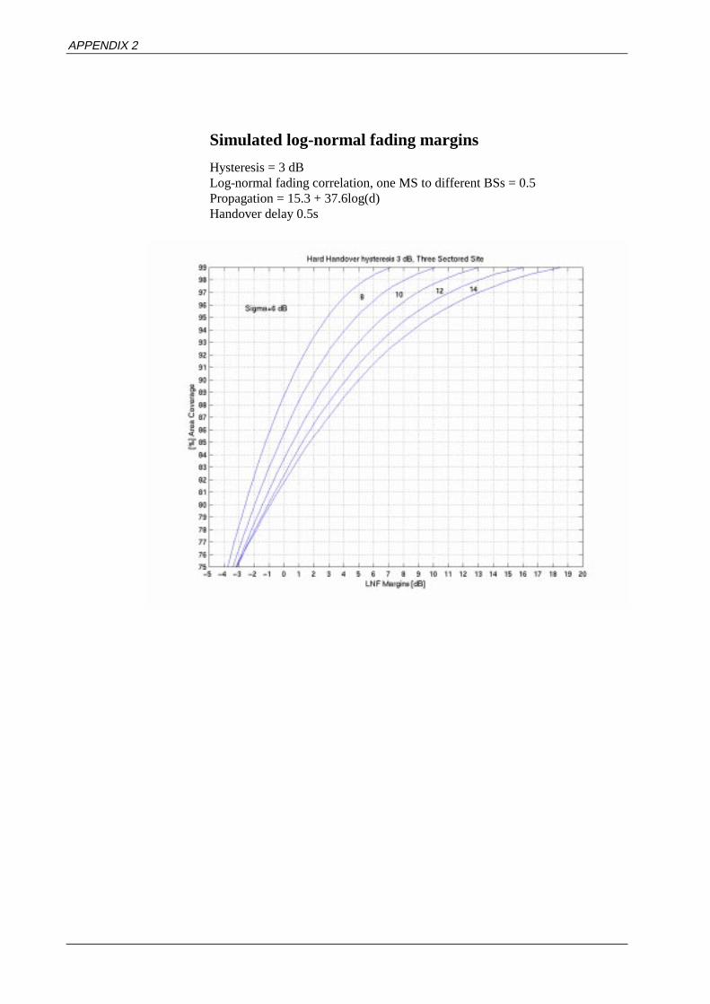
In order to find the log-normal fading margins in a multi-cell environment,simulations have been performed, see ref. 23 and Appendix 2.

The prerequisites for the simulations have been:

• 3 sectored sites

• correlation of log-normal fading between one MS and different BSs is 0.5

• lognormal fading correlation distance is 28.85 m

• the time to perform a handover is 0.5 s

The propagation environment is modeled with the Okumura-Hata formula asfollows:

Lpath = A + 10 logd [dB] where A=15.3 and =3.76,d[m].

Five different environments (σLNF = 6, 8, 10, 12, 14) have been studied. Theused handover hysteres in the simulations is 3dB. In order to find the requiredvalue of LNFmarg:

1. Choose the curve corresponding to fading environment in question .

2. On the X-axis, find the log-normal fading margin for the desired areacoverage (Y-axis).

Log-normal fading margins

Below the size of the log-normal fading margin is given for different types offading environments and area coverage. The values originate from thesimulations described above. A multi-cell environment with a handoverhysteresis of 3 dB is assumed.

Table 12. Log-normal fading margins (LNFmarg) in dB for differentenvironments.

Coverage [%]

σLNF [dB] 75 85 90 95 98

6 -3.7 -1.2 0.5 3.0 5.5

8 -3.4 -0.2 1.8 4.9 8.1

10 -3.1 0.7 3.2 6.8 10.7

12 -3.1 1.3 4.2 8.4 13.1

14 -3.2 1.8 5.1 9.9 15.3

These values are then used in Table 14 and Table 16, where design levels forvarious area types and coverage requirements are calculated.


10/100 56-100/FCP 103 1229/3 Rev A 2000-08-14 23(44)

4.2.3 InterferenceThe plain receiver sensitivity depends on the required carrier to noise ratio(C/N). When frequencies are reused, the received carrier power must be largeenough to combat both noise and interference, that means C/(N+I) mustexceed the receiver threshold. In order to get an accurate coverage predictionin a busy system, an interference margin (IFmarg) is defined.

The interference margin depends on the frequency reuse, the traffic load, thedesired percentage of area coverage and whether the uplink or the downlink isconsidered. Frequency hopping, dynamic power control and DTX reduce theinterference level. In a normal system an interference margin of 2 dB isrecommended.

Interference margin (IFmarg) = 2 dB

4.2.4 Body lossThe human body has several effects on the MS performance compared to afree standing mobile phone.

1. The head absorbs energy.

2. The antenna efficiency of some MSs can be reduced.

3. Other effects may be a change of the lobe direction and the polarization.These effects can be neglected in the link budget since 1) no mobileantenna gain is used and 2) X-polarized antennas are standard equipmenttoday. In this case the polarization loss is included in the downlink linkbudget and in the uplink, both polarizations can be received.

The body loss recommended by ETSI, ref. 20, is 3 dB for 1800 MHz.

Body loss (BL) = 3 dB

4.2.5 Car penetration lossWhen the MS is situated in a car without external antenna, an extra margin hasto be added in order to cope with the penetration loss of the car. This extramargin is approximately 6 dB, see ref. 24.

Car penetration loss (CPL) = 6 dB


24(44) 10/100 56-100/FCP 103 1229/3 Rev A 2000-08-14

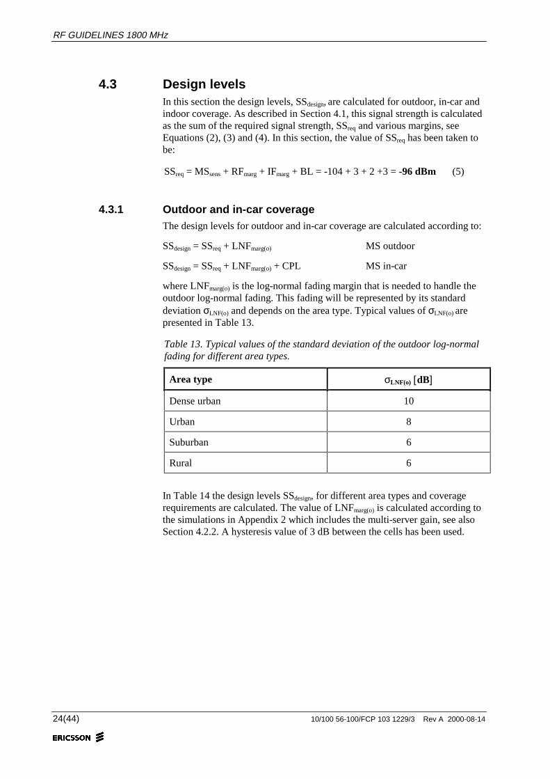
4.3 Design levelsIn this section the design levels, SSdesign, are calculated for outdoor, in-car andindoor coverage. As described in Section 4.1, this signal strength is calculatedas the sum of the required signal strength, SSreq and various margins, seeEquations (2), (3) and (4). In this section, the value of SSreq has been taken tobe:

SSreq = MSsens + RFmarg + IFmarg + BL = -104 + 3 + 2 +3 = -96 dBm (5)

4.3.1 Outdoor and in-car coverageThe design levels for outdoor and in-car coverage are calculated according to:

SSdesign = SSreq + LNFmarg(o) MS outdoor

SSdesign = SSreq + LNFmarg(o) + CPL MS in-car

where LNFmarg(o) is the log-normal fading margin that is needed to handle theoutdoor log-normal fading. This fading will be represented by its standarddeviation σLNF(o) and depends on the area type. Typical values of σLNF(o) arepresented in Table 13.

Table 13. Typical values of the standard deviation of the outdoor log-normalfading for different area types.

Area type σLNF(o) [dB]

Dense urban 10

Urban 8

Suburban 6

Rural 6

In Table 14 the design levels SSdesign, for different area types and coveragerequirements are calculated. The value of LNFmarg(o) is calculated according tothe simulations in Appendix 2 which includes the multi-server gain, see alsoSection 4.2.2. A hysteresis value of 3 dB between the cells has been used.


10/100 56-100/FCP 103 1229/3 Rev A 2000-08-14 25(44)

Table 14. Design levels for various area types and coverage requirements. A carpenetration loss (CPL) of 6 dB has been used.

Area type Coverage[%]

SSreq

[dBm]

LNFmarg(o)

[dB]

SSdesign

outdoor

[dBm]

SSdesign

in-car

[dBm]

75 -96 -3.1 -99.1 -93.1

85 -96 0.7 -95.3 -89.3

Dense urban 90 -96 3.2 -92.8 -86.8

σLNF(o) = 10 dB 95 -96 6.8 -89.2 -83.2

98 -96 10.7 -85.3 -79.3

75 -96 -3.4 -99.4 -93.4

Urban 85 -96 -0.2 -96.2 -90.2

σLNF(o) = 8 dB 90 -96 1.8 -94.2 -88.2

95 -96 4.9 -91.1 -85.1

98 -96 8.1 -87.9 -81.9

75 -96 -3.7 -99.7 -93.7

Suburban + 85 -96 -1.2 -97.2 -91.2

rural 90 -96 0.5 -95.5 -89.5

σLNF(o) = 6 dB 95 -96 3.0 -93 -87

98 -96 5.5 -90.5 -84.5

4.3.2 Indoor coverageDefinitions

Indoor coverageBy indoor coverage is understood the percentage of the ground floors of allthe buildings in the area where the signal strength is above the required signallevel of the mobiles, SSreq.

Building penetration lossBuilding penetration loss is defined as the difference between the averagesignal strength immediately outside the building and the average signalstrength over the ground floor of the building, see for instance ref. 25 andref. 26. The building penetration loss for different buildings is log-normallydistributed with a standard deviation; σBPL.

Variations of the loss over the ground floor could be described by a stochasticvariable, which is log-normally distributed with a zero mean value and astandard deviation of σfloor.


26(44) 10/100 56-100/FCP 103 1229/3 Rev A 2000-08-14

In this document σBPL and σfloor is lumped together by adding the two as werethey standard deviations in two independent log-normally distributedprocesses. The resulting standard deviation, σindoor or σLNF(i), could becalculated as the square root of the sum of the squares.

General

Indoor coverage in this document is about calculation of a required margin toachieve a certain indoor coverage in a fairly large area; large compared to theaverage macrocell size. It is assumed that it is the macrocells in the area thatprovides the major part of the indoor coverage. Hotspot microcells in the areawill of course improve on the indoor coverage but that effect is not covered inthis document.

The guidelines in this document regarding indoor coverage are not applicableto the case where the area of interest basically is covered by contiguousmicrocells and where macrocells only are used as umbrella cells.

It is common knowledge that the building penetration loss to floors higher upin the building in general decreases. This effect is known as height gain. Thisis actually an effect of the building penetration loss definition and not of thebuilding structure.

Indoor design level

The indoor design level is calculated according to (see Section 4.1):

SSdesign = SSreq + LNFmarg(o+i) + BPLmean MS indoor

where the sum of BPLmean and LNFmarg(o+i) can be seen as the indoor margin.BPLmean is the mean value of the building penetration loss and LNFmarg(o+i) isthe margin that is required to handle the total log-normal fading which arecomposed of both the outdoor log-normal fading (σLNF(o)) and the indoor log-normal fading σLNF(i).The total standard deviation of the log-normal fading isgiven by:

σLNF(o+i) = (σLNF(o)2

+ σLNF(i)2)½ (6)

In Table 15 some values of BPLmean, σLNF(o) and σLNF(i) are presented. These

figures are based on values presented in ref. 26 to ref. 30 and on experience.Note that the characteristics of different urban, suburban etc. environmentscan differ quite a lot over the world. Thus the values in Table 15 must betreated with restraint. They should be considered as a reasonableapproximation when no other information is obtainable. Rural areas are notconsidered in Table 15, since they are usually not designed for indoorcoverage.


10/100 56-100/FCP 103 1229/3 Rev A 2000-08-14 27(44)

Table 15. Some typical values of building penetration loss, and log-normalfading for different area types. These figures are based on values presented inref. 26 to ref. 30 and on experience.

BPLmean [dB] σLNF(o) [dB] σLNF(i) [dB] σLNF(o+i) [dB]

Dense urban 18 10 9 14

Urban 18 8 9 12

Suburban 12 6 8 10

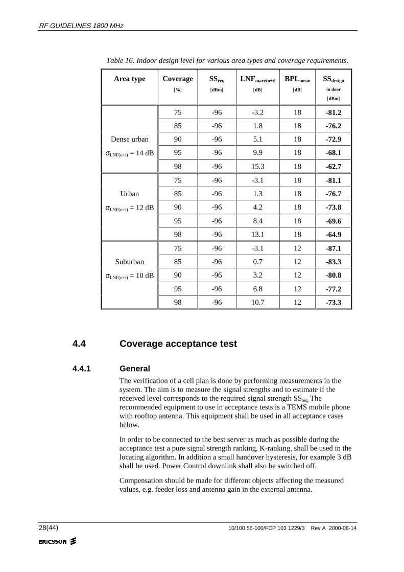
In Table 16 the design levels required to obtain 75%, 85%, 90%, 95% and98% indoor coverage are given.

The parameters for the building penetration and the log-normal fading aretaken to be those presented in Table 15.

The log-normal fading margins are given by the simulations in Appendix 2,see also Section 4.2.2. A multi cell environment has been assumed with ahysteresis value of 3 dB.


28(44) 10/100 56-100/FCP 103 1229/3 Rev A 2000-08-14

Table 16. Indoor design level for various area types and coverage requirements.


SSreq

[dBm]

LNFmarg(o+i)

[dB]

BPLmean

[dB]

SSdesign

in door

[dBm]

75 -96 -3.2 18 -81.2

85 -96 1.8 18 -76.2

Dense urban 90 -96 5.1 18 -72.9

σLNF(o+i) = 14 dB 95 -96 9.9 18 -68.1

98 -96 15.3 18 -62.7

75 -96 -3.1 18 -81.1

Urban 85 -96 1.3 18 -76.7

σLNF(o+i) = 12 dB 90 -96 4.2 18 -73.8

95 -96 8.4 18 -69.6

98 -96 13.1 18 -64.9

75 -96 -3.1 12 -87.1

Suburban 85 -96 0.7 12 -83.3

σLNF(o+i) = 10 dB 90 -96 3.2 12 -80.8

95 -96 6.8 12 -77.2

98 -96 10.7 12 -73.3

4.4 Coverage acceptance test

4.4.1 GeneralThe verification of a cell plan is done by performing measurements in thesystem. The aim is to measure the signal strengths and to estimate if thereceived level corresponds to the required signal strength SSreq. Therecommended equipment to use in acceptance tests is a TEMS mobile phonewith rooftop antenna. This equipment shall be used in all acceptance casesbelow.

In order to be connected to the best server as much as possible during theacceptance test a pure signal strength ranking, K-ranking, shall be used in thelocating algorithm. In addition a small handover hysteresis, for example 3 dBshall be used. Power Control downlink shall also be switched off.

Compensation should be made for different objects affecting the measuredvalues, e.g. feeder loss and antenna gain in the external antenna.


10/100 56-100/FCP 103 1229/3 Rev A 2000-08-14 29(44)

4.4.2 OutdoorThe acceptance level to verify is the required signal strength SSreq for outdoorcoverage. This level should be measured at least in A % of the samples, whereA represents the required area coverage.

Example 1. 95% outdoor coverage.

Criteria for downlink signal strength Rural, 95% outdoor coverage

Acceptance level, (SSreq) dBm or betterin 95 % of the samples

-96

4.4.3 In-carThe acceptance level to verify is the required signal strength SSreq for in-carcoverage. This level should be measured at least in A % of the samples, whereA represents the required area coverage.

Example 2. 95% in-car coverage

Criteria for downlink signal strength Rural, 95% in-car coverage

Acceptance level, (SSreq) dBm or betterin 95 % of the samples

-90

4.4.4 IndoorTo verify indoor coverage, subtract the outdoor log-normal fading marginLNFmarg(o) corresponding to the desired coverage (A%) from the SSdesign value.This level should be measured at least in A % of the samples.

Example 3. 95 % indoor coverage

Criteria for downlink signal strength Urban, 95% indoor coverage

SSdesign [dBm] -70

Acceptance level, (SSdesign- LNFmarg(o)

dBm) or better in 95 % of the samples -75


30(44) 10/100 56-100/FCP 103 1229/3 Rev A 2000-08-14

5 Cell planning

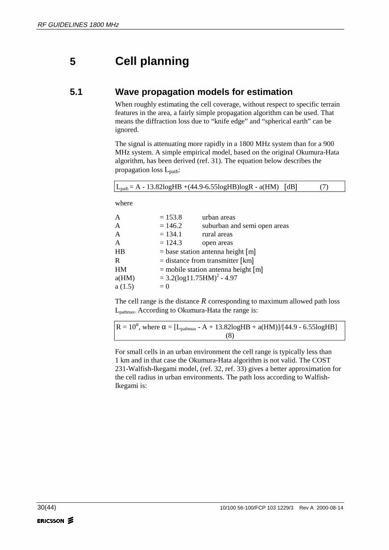
5.1 Wave propagation models for estimationWhen roughly estimating the cell coverage, without respect to specific terrainfeatures in the area, a fairly simple propagation algorithm can be used. Thatmeans the diffraction loss due to “knife edge” and “spherical earth” can beignored.

The signal is attenuating more rapidly in a 1800 MHz system than for a 900MHz system. A simple empirical model, based on the original Okumura-Hataalgorithm, has been derived (ref. 31). The equation below describes thepropagation loss Lpath:

Lpath = A - 13.82logHB +(44.9-6.55logHB)logR - a(HM) [dB] (7)

where

A = 153.8 urban areasA = 146.2 suburban and semi open areasA = 134.1 rural areasA = 124.3 open areasHB = base station antenna height [m]R = distance from transmitter [km]HM = mobile station antenna height [m]a(HM) = 3.2(log11.75HM)2 - 4.97a (1.5) = 0

The cell range is the distance R corresponding to maximum allowed path lossLpathmax. According to Okumura-Hata the range is:

R = 10α, where α = [Lpathmax - A + 13.82logHB + a(HM)]/[44.9 - 6.55logHB] (8)

For small cells in an urban environment the cell range is typically less than1 km and in that case the Okumura-Hata algorithm is not valid. The COST231-Walfish-Ikegami model, (ref. 32, ref. 33) gives a better approximation forthe cell radius in urban environments. The path loss according to Walfish-Ikegami is:


10/100 56-100/FCP 103 1229/3 Rev A 2000-08-14 31(44)

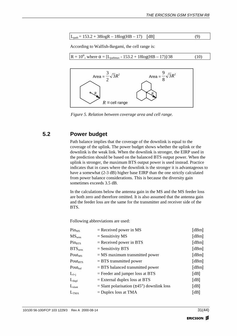
Lpath = 153.2 + 38logR – 18log(HB – 17) [dB] (9)

According to Walfish-Ikegami, the cell range is:

R = 10α, where α = [Lpathmax - 153.2 + 18log(HB – 17)]/38 (10)

9

83 2RArea =

R

3

23 2RArea =

cell rangeR =

R

Figure 5. Relation between coverage area and cell range.

5.2 Power budgetPath balance implies that the coverage of the downlink is equal to thecoverage of the uplink. The power budget shows whether the uplink or thedownlink is the weak link. When the downlink is stronger, the EIRP used inthe prediction should be based on the balanced BTS output power. When theuplink is stronger, the maximum BTS output power is used instead. Practiceindicates that in cases where the downlink is the stronger it is advantageous tohave a somewhat (2-3 dB) higher base EIRP than the one strictly calculatedfrom power balance considerations. This is because the diversity gainsometimes exceeds 3.5 dB.

In the calculations below the antenna gain in the MS and the MS feeder lossare both zero and therefore omitted. It is also assumed that the antenna gainand the feeder loss are the same for the transmitter and receiver side of theBTS.

Following abbreviations are used:

PinMS = Received power in MS [dBm]MSsens = Sensitivity MS [dBm]PinBTS = Received power in BTS [dBm]BTSsens = Sensitivity BTS [dBm]PoutMS = MS maximum transmitted power [dBm]PoutBTS = BTS transmitted power [dBm]Poutbal = BTS balanced transmitted power [dBm]Lf+j = Feeder and jumper loss at BTS [dB]Ldupl = External duplex loss at BTS [dB]Lslant = Slant polarisation (±45°) downlink loss [dB]LTMA = Duplex loss at TMA [dB]


32(44) 10/100 56-100/FCP 103 1229/3 Rev A 2000-08-14

Lpath = Path loss between MS and BTS [dB]Gant = Antenna gain in BTS [dBi]Gdiv = Diversity gain in BTS [dB]∆sens = MSsens − BTSsens [dB]

Downlink budget:

Downlink (DL) is the direction from the BTS to the MS. The downlink budgetgives the power level received in the MS.

Uplink budget:

Uplink (UL) is the direction from the MS to the BTS. The uplink budget givesthe power level received in the base station.

5.3 Power balance

5.3.1 Power balance with TMA at the antenna

BTS

Ext.dupl.

Feeder & jumpers TMA

MS

Lpath

LTMA

(Ldupl.) Gant, Gdiv, (Lslant)

Lf+j

TX ref.

RX ref.

Figure 6. System with TMA at the antenna. Ldupl should only be taken intoaccount if an external duplexer is used. Lslant should only betaken into accountif ±45° polarized TX antennas are used.

DL: PinMS = PoutBTS − Lf+j − (Ldupl) − LTMA + Gant − (Lslant) − Lpath (11)

UL: PinBTS = PoutMS − Lpath + Gant + Gdiv (12)

PinBTS is referenced to RX ref. point and PoutBTS is referenced to TX ref.point.

Assuming that the path loss is reciprocal, i.e. LpathUL = LpathDL. Then (11) and(12) give:


10/100 56-100/FCP 103 1229/3 Rev A 2000-08-14 33(44)

PoutBTS = PoutMS + Gdiv + Lf+j + LTMA + Ldupl + (Lslant) + PinMS − PinBTS

A balanced system is obtained when PinMS = PinBTS + ∆sens, where ∆sens =MSsens − BTSsens.

Poutbal = PoutMS + Gdiv + Lf+j + LTMA + (Ldupl) + (Lslant)+ ∆sens (13)

The corresponding EIRP is given by:

EIRP = Poutbal − Lf+j − (Ldupl) − LTMA+ Gant − (Lslant) (14)

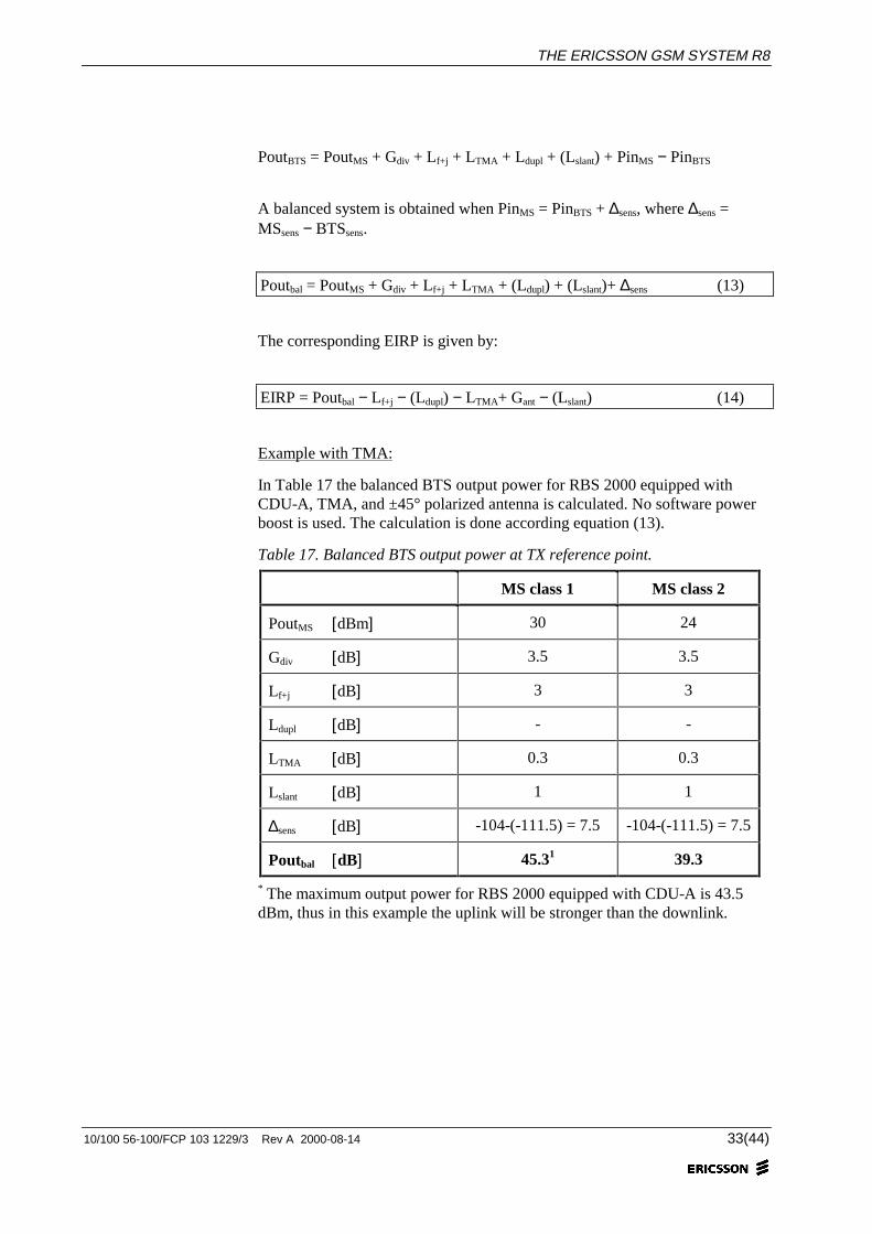
Example with TMA:

In Table 17 the balanced BTS output power for RBS 2000 equipped withCDU-A, TMA, and ±45° polarized antenna is calculated. No software powerboost is used. The calculation is done according equation (13).

Table 17. Balanced BTS output power at TX reference point.

MS class 1 MS class 2

PoutMS [dBm] 30 24

Gdiv [dB] 3.5 3.5

Lf+j [dB] 3 3

Ldupl [dB] - -

LTMA [dB] 0.3 0.3

Lslant [dB] 1 1

∆sens [dB] -104-(-111.5) = 7.5 -104-(-111.5) = 7.5

Poutbal [dB] 45.31 39.3

* The maximum output power for RBS 2000 equipped with CDU-A is 43.5dBm, thus in this example the uplink will be stronger than the downlink.


34(44) 10/100 56-100/FCP 103 1229/3 Rev A 2000-08-14

5.3.2 Power balance without TMA

BTS

Ext.dupl.

Feeder & jumpers

MS

Lpath(Ldupl.) Gant, Gdiv, (Lslant)

Lf+j

TX, RXref.

Figure 7. System without TMA at the antenna. Ldupl should only be taken intoaccount if an external duplexer is used. Lslant should only be taken intoaccount if ±45° polarized TX antennas are used.

DL: PinMS = PoutBTS− (Ldupl)− Lf+j + Gant − (Lslant) − Lpath (15)

UL: PinBTS = PoutMS − Lpath + Gant + Gdiv− Lf+j − (Ldupl) (16)

PinBTS and PoutBTS is the power in the TX and RX ref. point.

Assuming that the path loss is reciprocal, i.e. LpathUL = LpathDL. Then 15 and (16)give:

PoutBTS = PoutMS + Gdiv + (Lslant) + PinMS − PinBTS

A balanced system is obtained when PinMS = PinBTS + ∆sens, where ∆sens =MSsens − BTSsens.

Poutbal = PoutMS + Gdiv + (Lslant)+ ∆sens (17)

The corresponding EIRP is given by:

EIRP = Poutbal − (Ldupl) − Lf+j + Gant − (Lslant) (18)

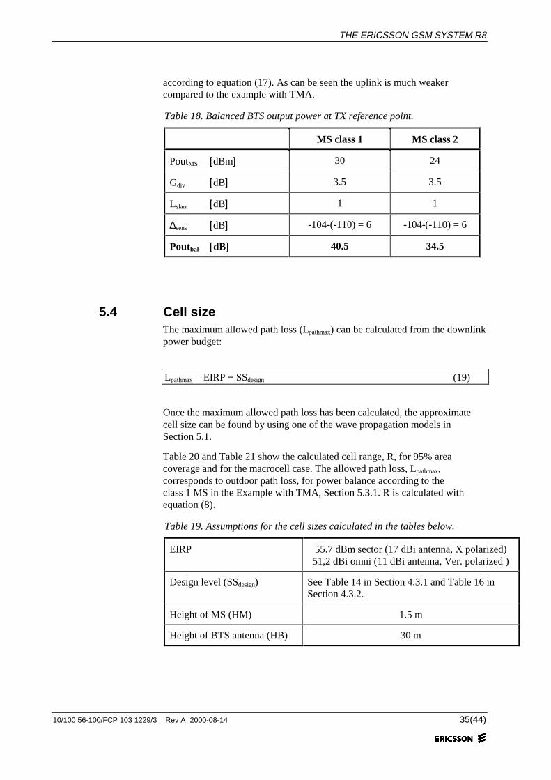
Example without TMA:

In Table 18 the balanced BTS output power for RBS 2000 equipped withCDU-A, and ±45° polarized antenna is calculated. The calculation is done


10/100 56-100/FCP 103 1229/3 Rev A 2000-08-14 35(44)

according to equation (17). As can be seen the uplink is much weakercompared to the example with TMA.

Table 18. Balanced BTS output power at TX reference point.

MS class 1 MS class 2

PoutMS [dBm] 30 24

Gdiv [dB] 3.5 3.5

Lslant [dB] 1 1

∆sens [dB] -104-(-110) = 6 -104-(-110) = 6

Poutbal [dB] 40.5 34.5

5.4 Cell sizeThe maximum allowed path loss (Lpathmax) can be calculated from the downlinkpower budget:

Lpathmax = EIRP − SSdesign (19)

Once the maximum allowed path loss has been calculated, the approximatecell size can be found by using one of the wave propagation models inSection 5.1.

Table 20 and Table 21 show the calculated cell range, R, for 95% areacoverage and for the macrocell case. The allowed path loss, Lpathmax,corresponds to outdoor path loss, for power balance according to theclass 1 MS in the Example with TMA, Section 5.3.1. R is calculated withequation (8).

Table 19. Assumptions for the cell sizes calculated in the tables below.

EIRP 55.7 dBm sector (17 dBi antenna, X polarized)51,2 dBi omni (11 dBi antenna, Ver. polarized )

Design level (SSdesign) See Table 14 in Section 4.3.1 and Table 16 inSection 4.3.2.

Height of MS (HM) 1.5 m

Height of BTS antenna (HB) 30 m


36(44) 10/100 56-100/FCP 103 1229/3 Rev A 2000-08-14

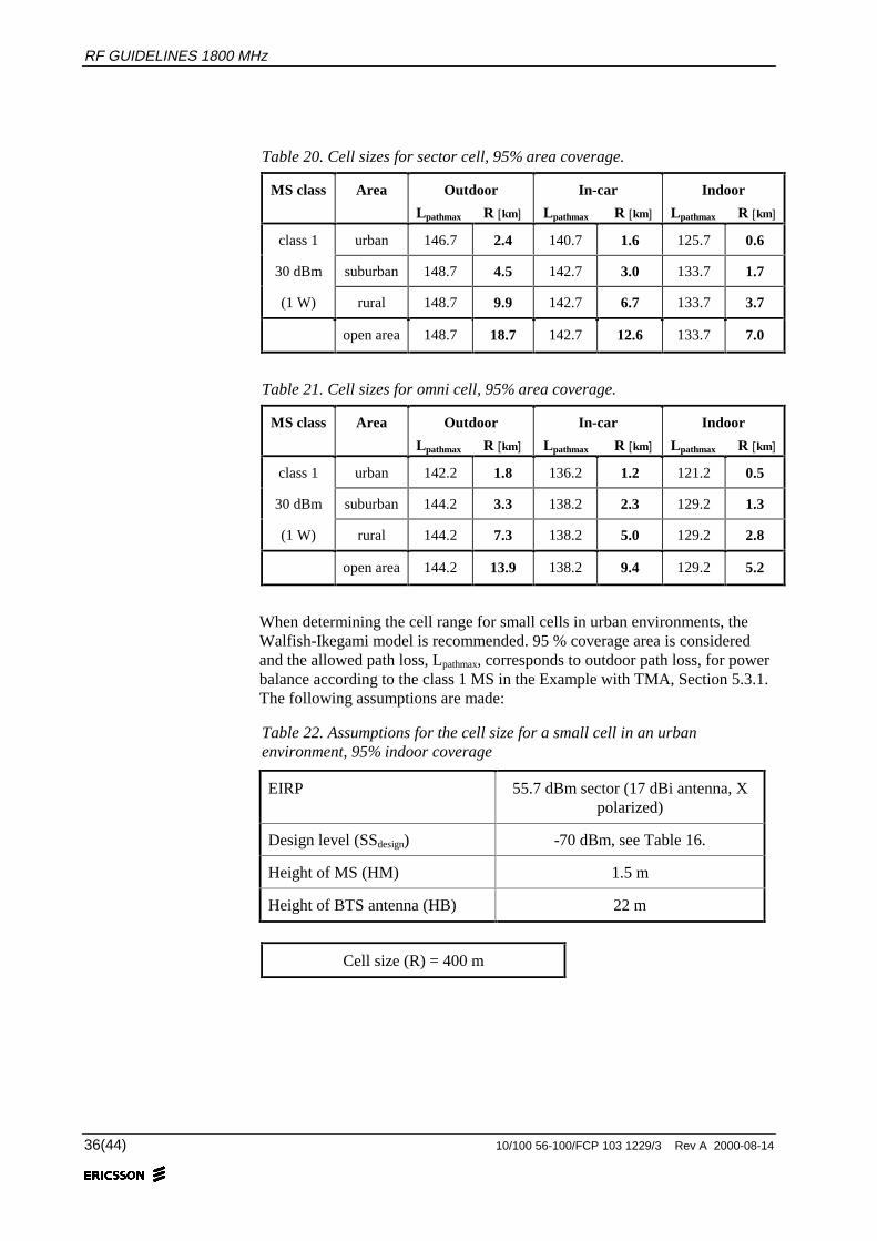
Table 20. Cell sizes for sector cell, 95% area coverage.

MS class Area Outdoor

Lpathmax R [km]

In-car

Lpathmax R [km]

Indoor

Lpathmax R [km]

class 1 urban 146.7 2.4 140.7 1.6 125.7 0.6

30 dBm suburban 148.7 4.5 142.7 3.0 133.7 1.7

(1 W) rural 148.7 9.9 142.7 6.7 133.7 3.7

open area 148.7 18.7 142.7 12.6 133.7 7.0

Table 21. Cell sizes for omni cell, 95% area coverage.

MS class Area Outdoor

Lpathmax R [km]

In-car

Lpathmax R [km]

Indoor

Lpathmax R [km]

class 1 urban 142.2 1.8 136.2 1.2 121.2 0.5

30 dBm suburban 144.2 3.3 138.2 2.3 129.2 1.3

(1 W) rural 144.2 7.3 138.2 5.0 129.2 2.8

open area 144.2 13.9 138.2 9.4 129.2 5.2

When determining the cell range for small cells in urban environments, theWalfish-Ikegami model is recommended. 95 % coverage area is consideredand the allowed path loss, Lpathmax, corresponds to outdoor path loss, for powerbalance according to the class 1 MS in the Example with TMA, Section 5.3.1.The following assumptions are made:

Table 22. Assumptions for the cell size for a small cell in an urbanenvironment, 95% indoor coverage

EIRP 55.7 dBm sector (17 dBi antenna, Xpolarized)

Design level (SSdesign) -70 dBm, see Table 16.

Height of MS (HM) 1.5 m

Height of BTS antenna (HB) 22 m

Cell size (R) = 400 m


10/100 56-100/FCP 103 1229/3 Rev A 2000-08-14 37(44)

6 References

ref. 1 “Sensitivity Figures and Output Power for RBS 2000 Macro”.LRN/X-98:033, Rev B, 1999.

ref. 2 “Sensitivity Figures and Output Power for RBS 2301 andRBS 2302”. LRU/X-98:068.

ref. 3 GSM 05.05 (Phase 2+), “Radio Transmission and Reception”,ETSI, version 8.3.0, 1999.

ref. 4 “RBS 2000 Description”, LR/X 98:122, Rev C, 1999

ref. 5 “Guideline for RBS Configuration in Macrocells”, LR/M-99:100,Rev B, 1999.

ref. 6 “RBS 2302 Description”, LRU/X-97:118, Rev C, 1998.

ref. 7 “RBS 2401 Description”, LRU/X-98:092, Rev B, 1999.

ref. 8 “RBS 2206 Description”, LRN/X-99:083, Rev B, 1999.

ref. 9 “CME 20 RBS 205 Description”, LR/X 95:174.

ref. 10 “Maxite Description”, LRU/X 97:012, Rev F, 1999.

ref. 11 Markku Maijala, “MS Sensitivity GSM900, GSM1800,GSM1900”, ERA/LVR/D-98:0162.

ref. 12 Compiled from product sheets and obtained from Hans Erneborg,KI/ERA/LRB/X.

ref. 13 Mats Samuelsson, “Summary of RBS 2000 RF Performance fromProduction Statistics (DCS 1800)”, LR/T-97:136, Rev B.

ref. 14 “Tower Mounted Amplifiers Guideline, the Ericsson’s GSMSystem R7”, 5/100 56-FCU 103 12 Uen, Rev B, 1999.

ref. 15 “Antenna Configuration Guidelines”, LV/R-97:029 Rev B.

ref. 16 Hansgård/Thiessen, “Slant Loss when Using X-polarizedAntennas”, LVR/D-97:293.

ref. 17 Mårten Eriksson, “Antenna Tilt Measurements at 1800 MHz,Kungsholmen, Stockholm”, LT/SN-95:308.

ref. 18 “Antenna Downtilt Guideline”, 1999


38(44) 10/100 56-100/FCP 103 1229/3 Rev A 2000-08-14

ref. 19 Hans Erneborg, “Repeaters in Cellular Systems”, LN/S-94:240.

ref. 20 GSM 03.30 (Phase 2+), “Radio Network Planning Aspects”, ETSI,version 8.3.0, 1999.

ref. 21 W.C. Jakes, Jr., “Microwave Mobile Communications”, JohnWiley & sons, New York, 1974 (p. 126).

ref. 22 Maria Thiessen, “Understanding Signal Coverage and Log-normalfading for a Single Cell”, LVR/D-99:0123.

ref. 23 N. Binucci, M. caselli, “Shadow Fading Margins for Omni, Threeand Six Sectored Sites”, TEI/TRB 00:006, 2000.

ref. 24 I.Kostanic, C.Hall, J.McCarthy, “Measurements of the VehiclePenetration Characteristics at 800 MHz”, Conference Proceeding,VTC 1998.

ref. 25 Andersson/Johansson, “Indoor Coverage from Macrocells at 900MHz and 1800 MHz”, LT/SN-94:649.

ref. 26 Anders Mattson, “Indoor coverage at 900 MHz”, BO/N-0043Rev B, 1990.

ref. 27 Jan Nordgren, “Byggnadsdämpning i 450 MHz-bandet”, T/R-8016,1987.

ref. 28 H.E. Walker, “Penetration of radio signals into buildings in thecellular radio environment”, B.S.T.J Vol. 62, No. 9, 1983.

ref. 29 A.M.D. Turkmani, “Radio propagation into buildings at 1.8 GHz”,COST231 TD(90) 117 Rev 1, 1991.

ref. 30 “Building penetration losses”, COST231 TD(90) 116 Rev 1, 1991.

ref. 31 Maria Thiessen, “An empirical Okumura-Hata based wavepropagation model for frequencies up to 3.5 GHz”,LVR/D:98:0320, Rev B, 1999.

ref. 32 “Urban transition loss models for mobile radio in the 900- and1800-MHz bands”, COST231 TD(90) 119 Rev 2, 1991.

ref. 33 Maria Thiessen, “Determining the cell radius in an urbanenvironment”, LVR/D-98:0391.

APPENDIX 1

Curves of Jakes formula

σ = standard deviation

= distance dependence

Cumulative normal function

70

80

90

0,5 0,7 0,9 1,1 1,3

F(x

), B

orde

r co

vera

ge [%

]

x

Log-normal fading margin= x×σ − HO gain

82

84

86

88

90

92

94

96

98

100

0 0,5 1 1,5 2 2,5 3 3,5 4

Border coverage

70 %

72 %

74 %

76 %

94 %92 %

90 %

86 %

84 %

78 %

80 %

82 %

88 %

σ/n [dB]

Are

a co

vera

ge [

%]

96 %98 %

1

Rn

APPENDIX 2

Simulated log-normal fading margins

Hysteresis = 3 dBLog-normal fading correlation, one MS to different BSs = 0.5Propagation = 15.3 + 37.6log(d)Handover delay 0.5s

APPENDIX 3

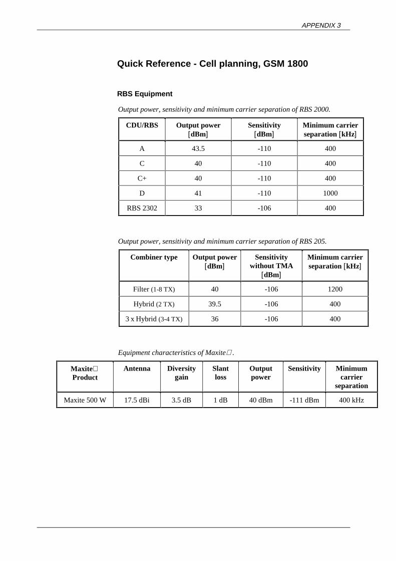
Quick Reference - Cell planning, GSM 1800

RBS Equipment

Output power, sensitivity and minimum carrier separation of RBS 2000.

CDU/RBS Output power[dBm]

Sensitivity[dBm]


A 43.5 -110 400

C 40 -110 400

C+ 40 -110 400

D 41 -110 1000

RBS 2302 33 -106 400

Output power, sensitivity and minimum carrier separation of RBS 205.

Combiner type Output power[dBm]

Sensitivitywithout TMA

[dBm]


Filter (1-8 TX) 40 -106 1200

Hybrid (2 TX) 39.5 -106 400

3 x Hybrid (3-4 TX) 36 -106 400

Equipment characteristics of Maxite.

MaxiteProduct

Antenna Diversitygain

Slantloss

Outputpower

Sensitivity Minimumcarrier

separation

Maxite 500 W 17.5 dBi 3.5 dB 1 dB 40 dBm -111 dBm 400 kHz

APPENDIX 3

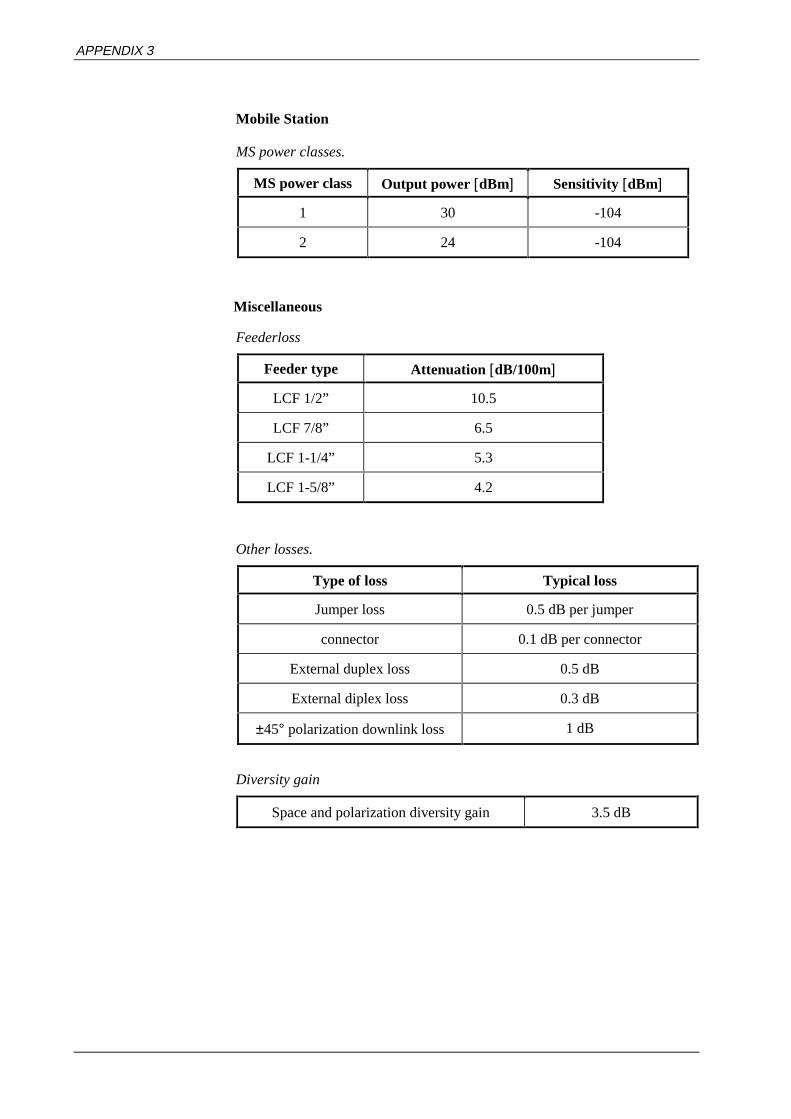
Mobile Station

MS power classes.

MS power class Output power [dBm] Sensitivity [dBm]

1 30 -104

2 24 -104

Miscellaneous

Feederloss

Feeder type Attenuation [dB/100m]

LCF 1/2” 10.5

LCF 7/8” 6.5

LCF 1-1/4” 5.3

LCF 1-5/8” 4.2

Other losses.

Type of loss Typical loss

Jumper loss 0.5 dB per jumper

connector 0.1 dB per connector

External duplex loss 0.5 dB

External diplex loss 0.3 dB

±45° polarization downlink loss 1 dB

Diversity gain

Space and polarization diversity gain 3.5 dB

APPENDIX 3

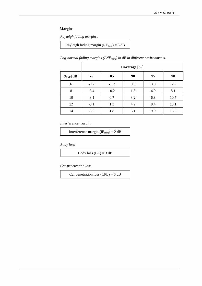
Margins

Rayleigh fading margin .

Rayleigh fading margin (RFmarg) = 3 dB

Log-normal fading margins (LNFmarg) in dB in different environments.

Coverage [%]

σLNF [dB] 75 85 90 95 98

6 -3.7 -1.2 0.5 3.0 5.5

8 -3.4 -0.2 1.8 4.9 8.1

10 -3.1 0.7 3.2 6.8 10.7

12 -3.1 1.3 4.2 8.4 13.1

14 -3.2 1.8 5.1 9.9 15.3

Interference margin.

Interference margin (IFmarg) = 2 dB

Body loss

Body loss (BL) = 3 dB

Car penetration loss

Car penetration loss (CPL) = 6 dB

APPENDIX 3

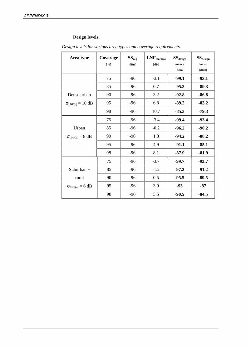
Design levels

Design levels for various area types and coverage requirements.


SSreq

[dBm]

LNFmarg(o)

[dB]

SSdesign

outdoor

[dBm]

SSdesign

in-car

[dBm]

75 -96 -3.1 -99.1 -93.1

85 -96 0.7 -95.3 -89.3

Dense urban 90 -96 3.2 -92.8 -86.8

σLNF(o) = 10 dB 95 -96 6.8 -89.2 -83.2

98 -96 10.7 -85.3 -79.3

75 -96 -3.4 -99.4 -93.4

Urban 85 -96 -0.2 -96.2 -90.2

σLNF(o) = 8 dB 90 -96 1.8 -94.2 -88.2

95 -96 4.9 -91.1 -85.1

98 -96 8.1 -87.9 -81.9

75 -96 -3.7 -99.7 -93.7

Suburban + 85 -96 -1.2 -97.2 -91.2

rural 90 -96 0.5 -95.5 -89.5

σLNF(o) = 6 dB 95 -96 3.0 -93 -87

98 -96 5.5 -90.5 -84.5

APPENDIX 3

Indoor design level for various area types and coverage requirements.


SSreq

[dBm]

LNFmarg(o+i)

[dB]

BPLmean

[dB]

SSdesign

in door

[dBm]

75 -96 -3.2 18 -81.2

85 -96 1.8 18 -76.2

Dense urban 90 -96 5.1 18 -72.9

σLNF(o+i) = 14 dB 95 -96 9.9 18 -68.1

98 -96 15.3 18 -62.7

75 -96 -3.1 18 -81.1

Urban 85 -96 1.3 18 -76.7

σLNF(o+i) = 12 dB 90 -96 4.2 18 -73.8

95 -96 8.4 18 -69.6

98 -96 13.1 18 -64.9

75 -96 -3.1 12 -87.1

Suburban 85 -96 0.7 12 -83.3

σLNF(o+i) = 10 dB 90 -96 3.2 12 -80.8

95 -96 6.8 12 -77.2

98 -96 10.7 12 -73.3

BTS output power for system balance with TMA at the antenna.

Poutbal = PoutMS + Gdiv + Lf+j + LTMA + (Ldupl) + (Lslant)+ ∆sens

EIRP = Poutbal − Lf+j − (Ldupl) − LTMA+ Gant − (Lslant)

BTS output power for system balance without TMA.

Poutbal = PoutMS + Gdiv + (Lslant)+ ∆sens

EIRP = Poutbal − (Ldupl) − Lf+j + Gant − (Lslant)

Documents

RF GUIDELINES 1800 A - cosconor.fr 1800MHz.pdf · RF GUIDELINES 1800 MHz THE ERICSSON GSM SYSTEM R8 ... parameter in the propagation model. General recommendations for …