Revisiting the omitted variables argument:Substantive vs. statistical adequacy

Aris Spanos

Abstract The problem of omitted variables is commonly viewed as a statisticalmisspecification issue which renders the inference concerning the influence of Xt

on yt unreliable, due to the exclusion of certain relevant factors Wt. That is,omitting certain potentially important factors Wt may confound the influence ofXt on yt. The textbook omitted variables argument attempts to assess theseriousness of this unreliability using the sensitivity of the estimatorb5(XiX)21Xiy to the inclusion/exclusion of Wt, by tracing that effect to thepotential bias/inconsistency of b. It is argued that the confounding problem is oneof substantive inadequacy in so far as the potential error concerns subject-matter,not statistical, information. Moreover, the textbook argument in termsof the sensitivity of point estimates provides a poor basis for addressing theconfounding problem. The paper reframes the omitted variables question intoa hypothesis testing problem, supplemented with a post-data evaluation ofinference based on severe testing. It is shown that this testing perspectivecan deal effectively with assessing the problem of confounding raised by theomitted variables argument. The assessment of the confouding effect usinghypothesis testing is related to the conditional independence and faithfulnessassumptions of graphical causal modeling.

Keywords: omitted variables, bias/inconsistency, confounding, robustness,sensitivity analysis, misspecification, substantive vs. statistical adequacy,structural vs. statistical models, severe testing

1 INTRODUCTION

Evaluating the effects of omitting relevant factors on the reliability of

inference constitutes a very important problem in fields like econometrics

where the overwhelming majority of the available data are observational in

nature. To place this problem in a simple context, consider estimating the

Linear Regression model:

M0 : yt~x>t bzut, ut*NIID 0, s2� �

, t~1, . . . , T , ð1Þ

where ‘i’ denotes the transpose of a vector/matrix, ut,NIID(0, s2) reads ‘ut

is distributed as a Normal, Independent and Identically Distributed (NIID)

process with mean 0 and variance s2’; (1) is viewed as explaining the

Journal of Economic Methodology 13:2, 179–218 June 2006

Journal of Economic Methodology ISSN 1350-178X print/ISSN 1469-9427 online

# 2006 Taylor & Francis http://www.tandf.co.uk/journals

DOI: 10.1080/13501780600730687

behavior of yt in terms of the exogenous variables in Xt - note that Xt

denotes the random vector and xt its observed value. The problem is

motivated by concerns that the estimated model M0 could have omitted

certain potentially important factors Wt, which may confound the influence

of Xt on yt. This contemplation gives rise to a potentially ‘true’ model:

M1 : yt~x>t bzw>t czet, et*NIID 0, s2� �

, t~1, . . . , T , ð2Þ

whose comparison with (1) indicates that inferences concerning the influence

of Xt on yt, based on M0, might be unreliable because one of the

assumptions of the error term, E(ut)50, is false. That is, in view of (2),

E utð Þ~w>t c=0.

These concerns are warranted because the multitude of potential factors

influencing the behavior of yt is so great that no logically stringent case can

be made that ‘all relevant factors have been included in Xt’. Indeed,

economic theories are notorious for invoking ceteris paribus clauses which

are usually invalid for observational data. As a result of this insuperable

obstacle, the problem is commonly confined to assessing the sensitivity

(fragility/robustness) of the estimator bb~ X>Xð Þ{1X>y to the inclusion/

exclusion of certain specific factors Wt as suggested by some theory/

conjecture. As such the issue is primarily one of substantive inadequacy in so

far as certain substantive subject-matter information raises the prospect that

certain influential factors might have been omitted from explaining the

behavior of yt, leading to misleading inferences.

The textbook omitted variables argument attempts to assess the sensitivity

of the estimator bb to the inclusion/exclusion of certain specific factors Wt, by

tracing the effects of these omitted variables to its bias/inconsistency; see

Johnston (1984), Greene (1997), Stock and Watson (2002), Wooldridge

(2003), inter alia. The sensitivity is often evaluated in terms of the difference in

the numerical values of the estimators of b in the two models (M0, M1). Large

discrepancies are interpreted as indicating the presence of bias, reflecting the

fragility of inference, which in turn indicates that a confounding problem

endangers the assessment of the real influence of Xt on yt.

The question posed in this paper is the extent to which the textbook omitted

variables argument can help shed light on this confounding problem. It is

argued that, as it stands, this argument raises a fundamental issue in empirical

modeling, but provides a rather poor basis for addressing it. The deficiency of

this argument stems from the fact that (a) the framing of the problem in terms

of the sensitivity of point estimators is inadequate for the task, and (b) the

problem concerning the relevance of omitted variables should be best viewed

as one of substantive, not statistical, inadequacy.

Broadly speaking, statistical adequacy concerns the validity of the

statistical model (the probabilistic assumptions constituting the model -

et,NIID(0, s2)) vis-a-vis the observed data. Substantive adequacy concerns

180 Articles

the validity of the structural model (the inclusion of relevant and the

exclusion of irrelevant variables, the functional relationships among these

variables, confounding factors, causal claims, external validity, etc.) vis-a-vis

the phenomenon of interest that gave rise to the data. The two premises are

related in so far as the statistical model provides the operational context in

which the structural model can be analyzed, but the nature of errors

associated with the two premises is very different. Moreover, a structural

model gains statistical ‘operational meaning’ when embedded into a

statistically adequate model. As argued below, this perspective suggests

that the sensitivity of point estimators provides a poor basis for assessing

either statistical or substantive inadequacies. A more effective assessment is

provided by recasting both, the substantive and statistical adequacy

problems, in terms of classical (frequentist) testing. However, the sensitivity

to statistical inadequacies is gauged in terms of the difference between

nominal and actual error probabilities, but the sensitivity to substan-

tive inadequacies could only be assessed in terms of statistical procedures

which can evaluate reliably the validity of claims concerning unknown

parameters.

2 THE OMITTED VARIABLES ARGUMENT REVISITED

For reference purposes, let us summarize the textbook omitted variables

argument, as a prelude to the critical discussion that follows. The ugliness of

the matrix notation is needed in order to point out some crucial flaws in the

argument.

2.1 Summary of the textbook argument

Consider a situation where the following Linear Regression model was

estimated:

M0 : y~Xbzu, u*N 0, s2IT

� �, ð3Þ

where y:T61, X:T6k, IT :T6T (identity matrix), but the ‘true’ model is:

M1 : y~XbzWcze, e*N 0, s2IT

� �, ð4Þ

where W:T6m. The question posed is how the ‘optimal’ properties of the

least squares estimators (bbb, s2):

bbb~ X>X� �{1

X>y, s2~1

T{kbuu>buu, ð5Þ

of (b, s2), respectively, are affected by ‘omitting’ the variables W from (3).

Substituting the ‘true’ model (4) into the estimator bbb and taking

expectations (E(.)) and limits in probability ( limT??

), one can show that, in

Revisiting omitted variables 181

general, bbb is a biased and inconsistent estimator of b:

E bbb� �

~bz X>X� �{1

X>Wc,

limT??

bbb� �

~bz limT??

X>X� �

=T� �{1

X>W� �

=T� �

c� �

,ð6Þ

assuming that limT??

X>WT

� �~Cov Xt, Wtð Þ=0. Similarly, given that:

buu~y{Xbbb~MX Wczeð Þ, where MX~I{X X>X� �{1

X>,

s2 will, in general, be a biased and inconsistent estimator of s2:

E s2� �

~s2z1

T{kc>W>MXWc

� �,

limT??

s2� �

~s2z limT??

c>W> MX=TÞWcð �: ð7Þ�

It is interesting to note that the bias/inconsistency of (bbb, s2) vanishes when

c50, but that of bbb also vanishes when Cov(Xt, Wt)50. As shown below, c50

and Cov(Xt, Wt)50 are not equivalent.

The impression given by the textbook omitted variables argument is that

the difference between the numerical values of the two estimators:

bbb~ X>X� �{1

X>y, ebb~ X>MW X� �{1

X>MW y,

arising from (3) and (4), respectively, provide a way to assess this sensitivity.

The rationale behind this view is that, since:

bbb~bz X>X� �{1

X> Wczeð Þ, ebb~bz X>MW X� �{1

X>MW e,

(bbb{ebb)^ X>X� �{1

X>Wc,ð8Þ

the value of (bbb{ebb) reflects the bias/inconsistency. As argued in the sequel,

(8) provides very poor grounds for assessing the presence/absence of

estimation bias.

2.2 A preliminary critical view

Let us take a preliminary look at the textbook omitted variables argument

as a way to assess the sensitivity (fragility/robustness) of the estimator bb vis-

a-vis the presence of potentially relevant factors Wt.

First, the omitted variables argument does not distinguish between

statistical and substantive inadequacy. Indeed, by calling it ‘specification

error’, the textbook interpretation gives the clear impression that the issue is

one of statistical misspecification, i.e., ‘all relevant factors have been in-

cluded in Xt’ forms an integral part of the statistical premises; see Johnston(1984). It what follows, it is argued that the statistical premises include no

182 Articles

such assumption. The problem of confounding is an issue of substantive

inadequacy because it concerns the probing for errors in bridging the gap

between the structural model and the phenomenon of interest.

The confusion between the statistical and structural premises arises

primarily because the textbook specification of a statistical model is given in

terms of the error term: u,N(0, s2IT). This, in turn, imposes a substantive

perspective on the statistical analysis which often leads to confusions; see

Spanos and McGuirk (2002). Instead, the substantive and statistical

perspectives should be viewed as two separate but complemental stand-

points. As argued in Spanos (1986), the error assumptions provide a

somewhat misleading and incomplete picture of the probabilistic structure

indirectly imposed on the observable random variables involved; the only

structure that matters for statistical inference purposes. In order to provide

a more well-defined statistical perspective, and draw the line between the

statistical and substantive premises more clearly, Spanos (1986) proposed a

recasting of the probabilistic assumptions of the error term into assumptions

concerning the distribution of the observable random variables involved

D(yt|Xt; h). The recasting revealed that assumptions [1]–[4] (see Table 1) are

equivalent to the error assumptions (ut|Xt5xt),NIID(0, s2), t g (see

table 2), where :5{1, 2, …, T, …} (‘:5’ denotes ‘is defined as’) is an index

set with t often, but not exclusively, indicating time. (The index could also

refer to the order of cross-section data.)

Assumption [5], however, turns out to be ‘veiled’ because it is not entailed

by assumptions (1)–(4), even though it is (implicitly) part of the statistical

Table 1 The Normal/Linear Regression Model

Statistical GM: yt~b0zb>1 xtzut, t [ ,

[1] Normality: (yt|Xt5xt),N(.,.),[2] Linearity: E ytjX t~xtð Þ~b0zb>1 xt, linear in xt,[3] Homoskedasticity: Var(yt|Xt5xt)5s2, free of xt,[4] Independence: {(yt|Xt5xt), t g } is an independent

process,[5] t-invariance: h:5(b0, b1, s2) do not vary with t.

b0 : ~m1{b>1 m2, b1 : ~S{122 s21, s2 : ~s11{s>21S{1

22 s21.

m15E(yt), m25E(Xt), s115Var(yt), s215Cov(Xt, yt), S225Cov(Xt).

Table 2 Equivalence of Probabilistic Assumptions

Process {(ut|Xt5xt), t g } vs. Process {(yt|Xt5xt), t g }

(1) (ut|Xt5xt),N(.,.) u [1] (yt|Xt5xt),N(.,.),(2) E(ut|Xt5xt)50 u [2] E ytjXt~xtð Þ~b0~b>1 xt,(3) E u2

t Xtj ~xt� �

~s2 u [3] Var(yt|Xt5xt)5s2,

(4) Independent over t g u [4] Independent over t g .

Revisiting omitted variables 183

premises. Note that the homoskedasticity assumption [3] refers to

Var(yt|Xt5xt) being free of xt, not t. Hence, statistical inadequacy for the

Linear Regression model concerns departures from assumptions [1]–[5]only; no assumption concerning the inclusion of all ‘relevant’ variables in Xt

is made by the statistical premises – it is part of the structural premises.

As argued in section 3, when the statistical premises of the models M0 and

M1 are respecified in terms of the observable random variables involved (see

Table 1), it becomes clear that the claim ‘bbb is a bad estimator of the

structural parameter b (reflecting the effect of Xt on yt)’, constitutes a highly

equivocal assertion. The (statistical) operational meaning of b in M0 is

different from that in M1, say a, where, in general, b?a. Similarly, the

conditional variances of the two models M0 and M1 are also different, say s20

and s21, respectively; see section 3.2.

To simplify the preliminary discussion let us consider the case where Xt is

a single variable and one is interested in the sensitivity of the estimated

coefficient b with respect to the inclusion of a potentially relevant set of

variables Wt by comparing the following two models:

M0 : yt~d0zxtbze1t, e1t*NIID 0, s20

� �, t [ ,

M1 : yt~d1zxtazw>t cze2t, e2t*NIID 0, s21

� �, t [ :

ð9Þ

The idea behind the omitted variables argument is that when the numerical

values of the two least-squares estimators, say bbb and baa, corresponding to

models (M0, M1), are similar, the estimator bbb will be robust to the omitted

variables Wt, and thus reliable; otherwise the inference is considered fragile

and unreliable; see Leamer (1978), Leamer and Leonard (1983). Although

this argument appears to be intuitively obvious, on closer examination itturns out to be seriously flawed. Assessing the sensitivity (fragility/

robustness) of inference in terms of the observed difference (bbb{baa) leaves

a lot to be desired in addressing the substantive unreliability issue raised by

the omitted variables problem. It is demonstrated below that this strategy is

ineffective in assessing the reliability of either statistical or substantive

inferences. Moreover, it is important to emphasize that the reliability of

statistical inferences is assessed using error probabilities, not sensitivityanalysis, and the reliability of substantive claims can only be properly

assessed by using reliable testing procedures, as opposed to point estimation

fragility arguments.

2.2.1 The sensitivity of frequentist statistical inference

The sensitivity of (frequentist) inference to departures from the statistical

premises is not measured in terms of parameter estimates and their

numerical differences, or/and by attaching probabilities to different valuesof the unknown parameters as in Bayesian inference; see Leamer (1978). It is

184 Articles

appraised via changes in the method’s trustworthiness: its capacity to give

rise to valid inferences. This is calibrated in terms of the associated error

probabilities: how often these procedures lead to erroneous inferences. In thecase of confidence-interval estimation the calibration is commonly gauged in

terms of minimizing the coverage error probability: the probability that the

interval does not contain the ‘true’ value of the unknown parameter. In the

case of hypothesis testing the calibration is ascertained in terms of

minimizing the type II error probability: the probability of accepting the

null hypothesis when false, for a given type I error probability; see Cox and

Hinkley (1974).

In the presence of departures from the model assumptions, the differencebetween the nominal (based on the assumed premises) and actual (based on

the actual premises) error probabilities provides a measure of the sensitivity

of inference to such departures; see Spanos (2005a). For example, if the

nominal type I error probability of a t-test is 5 per cent, but the actual turns

out to be 95 per cent, the sensitivity of inference is very high and the

inference based on such a test is said to be fragile; if the nominal and actual

error probabilities are, say 5 per cent and 7 per cent, respectively, the test is

said to be robust. It should be noted that changes in type II errorprobabilities (or power) are also an integral part of the assessment of the

test’s sensitivity; see Spanos (2005a).

2.2.2 The limited scope of the estimated difference (bb{aa)

For the sake of the preliminary discussion that follows, let us assume that

both models (M0, M1) are statistically adequate. It is argued below that this

is a crucial assumption which, when false, will invalidate the whole analysis.The first problem with the omitted variables argument is that the

estimated difference (bb{aa), by itself, provides poor grounds for assessing

the similarity between the underlying unknown parameters (b, a), and even

poorer grounds for assessing the relevance of the omitted variables Wt; i.e.

c50. Let us look at this in some detail.

Consider two estimates bb~:796 and aa~:802 which are close in numerical

values; (bb{aa)~{:06. Viewed in the context of the omitted variables

argument these estimates are likely to be interpreted as indicating that theomitted variables bias is rather small and thus immaterial, ensuring the

robustness of any inference based on bb. In what follows we will consider

three different scenarios, which are based on the same estimates but license

diametrically different conclusions.

In scenario 1 the estimates bb~:796, aa~:802 are supplemented with their

estimated standard errors SE(bb)~:012 and SE aað Þ~1:2, and the informa-

tion that the coefficients of Wt are significantly different from zero (c?0) on

the basis of a joint 5% significance level F-test. (Note that both the standarderrors and the F-test require estimating the variances (s2

0, s21).) In this case

Revisiting omitted variables 185

the estimators (bb, aa) give rise to completely dissimilar inferences concerning

the effect of Xt on yt. The t-ratios t bð Þ~ :796:012 ~66:3 :000½ �, and

t að Þ~ :8021:2 ~:668 :504½ � with the p-values in square brackets, can be

interpreted as indicating support for the claims (a) 0,b(.82, and (b)

a50. Interpreted in the context of the substantive reliability issue, scenario 1

seems to suggest that the relationship between yt and Xt in M0 is spurious

because in the presence of Wt, Xt becomes redundant.

In scenario 2, the same estimates (bb~:796, aa~:802) are supplemented

with different estimated standard errors SE(bb)~:012, SE aað Þ~:010, and the

information that the coefficients of Wt are not significantly different from

zero (i.e. c50) on the basis of a joint 5 per cent significance level F-test.Given that t bð Þ~ :796

:012 ~66:3 :000½ �, and t að Þ~ :802:01 ~80:2 :000½ �, the evidence

might be interpreted as indicating a non-spurious relationship which is

robust to the inclusion of other potentially relevant variables; the exact

opposite to the conclusions in scenario 1.

In scenario 3 we retain the same estimates (bb~:796, aa~:802) and

standard errors (SE(bb)~:012, SE aað Þ~:010) as in scenario 2, but c?0

on the basis of a joint 5 per cent significance level F-test. This informa-

tion seems to indicate a substantive relationship between yt and Xt whichcaptures the systematic information in the behavior of yt, but at the same

time Wt seems to be relevant. How can one interpret such evidence? As

argued below, for a proper interpretation of these evidence one needs to

investigate the relationship between Xt and Wt, and in particular the claim

Cov(Xt, Wt)50.

The above discussion indicates that on the basis of the same point

estimates of the effect of Xt on yt, bb~:796 and aa~:802, very different

substantive inferences can be drawn depending on other informationrelating to the estimated statistical models, including the statistics SE(bb) and

SE aað Þ and the parameters c and Cov(Xt, Wt).

By the same token, two numerically dissimilar point estimates bb~:796and aa~:532, where (bb{aa)~:264, might provide support for similar claims

concerning the underlying ‘true’ b. Viewed in the context of the omitted

variables argument, the apparent discrepancy between the two estimates will

be interpreted as indicating that the omitted variables bias is substantial.

This argument, however, can be very misleading because, if we combinethese estimates with SE(bb)~:012 and SE aað Þ~:144 to define scenario 4, the

evidence seems to support the claim 0,b(.82, as in scenario 1. How these

claims are substantiated using severe testing reasoning (see Mayo, 1996)

will be discussed in section 4.2. At this stage it suffices to state that

such claims cannot be legitimated on the basis of confidence-interval

estimation.

In summary, viewing the problem as one of omitted variables bias for bband revolving around the difference in the numerical values of the two pointestimates bb and aa, does not do justice to the problem of assessing the

186 Articles

substantive reliability issue. As the above scenarios 1–4 indicate, for a more

informative assessment of the relationship between yt and Xt and the role ofWt, one needs additional information concerning the other parameters c, s2

1

and Cov(Xt, Wt). A more informative perspective is provided by hypothesis

testing where the emphasis is placed on warranted claims concerning these

parameters in light of the data; see section 4.

2.2.3 Statistical inadequacy and the assessment of substantive claims

This brings up the second problem with the textbook omitted variables

argument. Given that any assessment of substantive reliability relies on

statistical inference procedures, such as estimation and testing, statistical

adequacy constitutes a necessary condition for such an assessment to be

reliable. Statistical inferences such as (a) 0,b(.82, and (b) a50 in scenario

1 above, depend crucially on the validity of the probabilistic assumptions

[1]–[5]; see Table 1. When any of these assumptions is invalid the statistical

procedures cannot be relied upon to assess the substantive reliability issue in

question. For instance, if assumption [5] in M0 is false, say d0 is not t-

invariant, but instead:

d0 tð Þ~m0zm1t, ð10Þ

and the omitted variables Wt are trending, then c is likely to appear

statistically significant in M1 (i.e. c?0), irrespective of its substantive

significance. This is because Wt will act as a proxy for the missing (m1t); Wt

need not have the same trending structure to appear statistically significant.

This suggests that before one can draw valid substantive inferences

concerning the sensitivity of b or whether the additional factors in Wt play

a significant role in explaining the behavior of yt, one should ensure the

statistical adequacy of the estimated model M1 for data (y, x, W); see Mayoand Spanos (2004).

The need to distinguish between substantive and statistical reliability

assessments raises the problem of delineating the two issues to avoid

Duhemian problems for apportioning blame. In order to indicate how such

problems arise in theory testing more generally, let us consider the followingsimple modus tollens argument for falsifying a theory, where a theory T is

embedded in a statistical model S entailing evidence e:

If T and S, then e

not-e,

hnot-T or not-S

It is clear from this argument that one cannot distinguish between not-T (the

theory is false) and not-S (the statistical model is misspecified) when not-e is

observed. However, if one is able to establish the statistical adequacy of S

(separate from the adequacy of T), then the above argument can be

Revisiting omitted variables 187

modified to yield a deductively valid argument for falsifying a theory:

If T and S, then e

S & not-e,

hnot-T

Returning to the omitted variables argument, T denotes model M0, S standsfor model M1 and the presence/absence of Wt should be viewed as a

substantive issue posed in the context of M1, assuming that the latter is

statistically adequate. Because of the necessity of ensuring the statistical

adequacy of S, substantive and statistical adequacy assessments are very

different in nature and are posed in the context of different models, the

structural (M0) and statistical (M1), respectively.

In the next section it is argued that the best way to assess substantive

adequacy is to view the structural model as embedded into a statistical

model, with the two models retaining their own ontology, despite the fact

that sometimes they seem to coincide, or take on different roles depending

on the nature of the question posed.

3 THE PROBABILISTIC REDUCTION PERSPECTIVE

The aim of this section is to provide a summary of the ProbabilisticReduction framework in the context of which the problems and issues raised

above in relation to the textbook omitted variables argument can be

delineated and addressed. An important feature of this framework is the

sequence of interrelated models (theory, structural, statistical and empiri-

cal), which are used to bridge the gap between a theory and data; see Spanos

(1986, 1989, 1995a, 2005c). This sequence of models is in the spirit of the

hierarchy of models (primary, experimental, data) proposed by Mayo

(1996), ch. 5, designed to ‘localize’ the probing for different types of errorsarising at different levels of empirical modeling; see Spanos (2006c). In the

discussion that follows we focus primarily on distinguishing between

structural and statistical models and their associated errors in an attempt to

place the omitted variables argument in a proper perspective and separate

the substantive from the statistical adequacy issues.

3.1 Structural vs. statistical models

In an attempt to distinguish more clearly between the statistical and

substantive perspectives we briefly discuss the nature and ontology ofstructural and statistical models in empirical modeling; see Spanos (2005d)

for a more detailed discussion.

It is widely recognized that most economic phenomena are influenced by

a very large number of contributing factors, and that explains why economictheories are dominated by ceteris paribus clauses. The idea behind

188 Articles

postulating a theory is that in explaining the behavior of an economic

variable, say yk, one demarcates the segment of reality to be modeled by

selecting the primary influencing factors xk, cognizant of the fact that there

might be numerous other potentially relevant factors jk (observable and

unobservable) that jointly determine the behavior of yk via:

yk~h� xk, jkð Þ, k [ ¥, ð11Þ

where h*(.) represents the true behavioral relationship for yk. The guiding

principle in selecting the variables in xk is to ensure that they collectively

account for the systematic behavior of yk, and the unaccounted factors jk

represent non-essential disturbing influences which have only a non-

systematic effect on yk. This line of reasoning gives rise to a structural

(estimable) model of the form:

yk~h xk; wð Þze xk, jkð Þ, k [ ¥, ð12Þ

where h(.) denotes the postulated functional form, w stands for the structural

parameters of interest, and e(xk, jk) represents the structural error term,

viewed as a function of both xk and jk. By definition the error term process

is:

e xk, jkð Þ~yk{h xk; wð Þ, k [ ¥f g, ð13Þ

and represents all unmodeled influences, intended to be a white-noise (non-

systematic) stochastic process {e(xk, jk), k gN} satisfying the properties:

ið Þ E e xk, jkð Þð Þ~0,

iið Þ E e xk, jkð Þ:e x‘, j‘ð Þð Þ~ s2,

0,

k~‘

k=‘, k, ‘[¥,

(

iiið Þ E e xk, jkð Þ:h xk; wð Þð Þ~0,

9>>>>=

>>>>;

V xk, jkð Þ[¡x|¡j:ð14Þ

In summary, a structural model provides an ‘idealized’ substantive

description of the phenomenon of interest, in the form of a ‘nearly isolated’

mathematical system; see Spanos (1986). As such, a structural model (a)

influences the demarcation of the segment of reality to be modeled, (b)

suggests the aspects of the phenomenon to be measured, with a view to (c)

‘capture’ the systematic (recurring) features of the phenomenon of interest

giving rise to data Z:5(z1, z2, …, zn). The kind of errors one should probe

for in the context of a structural model concern the bridging of the gap

between the phenomenon of interest and the assumed structural model.

These concerns include the form of h(xk; w) and the circumstances that

render the error term e(xk, jk) potentially systematic, such as the presence of

relevant factors, say wk in jk, that might have a systematic influence on the

behavior of yt.

It is important to emphasize that (12) depicts a ‘factual’ generating

mechanism, which aims to approximate the actual data generating

Revisiting omitted variables 189

mechanism. As the assumptions (i)–(iii) of the structural error stand, are

statistically non-testable because their assessment involves the unspecified/

unobserved jk. To render (i)–(iii) statistically testable one needs to embed

this structural model into a statistical one. Not surprisingly, the nature of

the embedding itself depends crucially on whether the data Z:5(z1, z2, …,

zn) are the result of an experiment or they are non-experimental

(observational) in nature. To bring out the vulnerability to the problem of

omitted variables when modeling with observational data, we need to

compare the two cases.

3.1.1 Experimental data

In the case where one can perform experiments, ‘experimental design’

techniques (such as randomization, blocking and replication), might allow

one to operationalize the ‘near isolation’ condition, including the ceteris

paribus clauses. The objective is to ensure that the error term is no longer a

function of (xk, jk), but for all values (xk, jk) gRx6Rj:

e xk, jkð Þ~ek*NIID 0, s2� �

, k~1, . . . , n: ð15Þ

For instance, randomization and blocking are often used to ‘neutralize’ and

‘isolated’ the phenomenon from the potential effects of jk by ensuring that

the uncontrolled factors cancel each other out; see Fisher (1935).

As a direct result of the experimental ‘control’ via (15) the structural

model (12) is essentially transformed into a statistical model:

yk~h xk; hð Þzek, ek*NIID 0, s2� �

, k~1, 2, . . . , n, ð16Þ

where the statistical error term ek in (16) is qualitatively very different from

the structural error term e(xk, jk) in (12) because ek is no longer a function of

jk. For more precise inferences one needs to be more particular about the

probabilistic assumptions defining the statistical model, including the

functional form h(.). This is because the more finical the probabilistic

assumptions (the more constricting the statistical premises), the more precise

the inferences.

The most important aspect of embedding the structural (12) into the

statistical model (16) is that, in contrast to (i)–(iii) in (14), the probabilistic

assumptions concerning the statistical error term ek are rendered testable. By

operationalizing the ‘near isolation’ condition via (15), the error term has

been tamed and (16) can now be viewed as a statistical generating mechanism

that ‘schematically’ describes how the data (y1, y2, …, yn) could have been

generated using (x1, …, xn) in conjunction with pseudo-random numbers for

(e1, e2, …, en). In principle, when the probabilistic assumptions constituting

the statistical model in question are valid, one is able to use (16) to simulate

‘faithful replicas’ of the data (y1, y2, …, yn).

190 Articles

The ontological status of the statistical model (16) is different from that of

the structural model (12) in so far as (15) has operationalized the ‘near

isolation’ condition. The statistical model has been ‘created’ as a result of

the experimental design/control. As a consequence of (15) the informational

universe of discourse for the statistical model (16) has been confined to the

probabilistic information relating to the observables Zk:5(yk, Xk). The

‘taming’ of the error term using (15) has introduced the probabilistic

perspective, which considers data Z:5(z1, …, zn) as a ‘realization’ of a

(vector) stochastic process {Zt, t g } whose probabilistic structure is such

that would render data Z a ‘truly typical’ realization thereof. This

probabilistic structure, according to Kolmogorov’s theorem, can be fully

described, under certain mild regularity conditions, in terms of the joint

distribution D(Z1, Z2, …, ZT; w); see Doob (1953). It turns out that a

statistical model can be viewed as a parameterization of the presumed

probabilistic structure of {Zt, t g }, arising as a reduction from this joint

distribution; see Spanos (2006c).

In summary, a statistical model constitutes an ‘idealized’ probabilistic

description of a stochastic process {Zt, t g }, giving rise to data Z, in

the form of an internally consistent set of probabilistic assumptions,

chosen to ensure that this data represent a ‘truly typical realization’ of {Zt,

t g }.

In contrast to a structural model, which relies on substantive subject

matter information, a statistical model relies on the statistical information in

D(Z1, Z2, …, ZT; w), that ‘reflects’ the chance regularity patterns exhibited

by the data. Hence, once Zt is chosen, a statistical model takes on ‘a life of

its own’ in the sense that it constitutes a self-contained data generating

mechanism defined exclusively in terms of probabilistic assumptions

pertaining to the observables Zk:5(yk, Xk). An important example of such

a statistical model arises when h(.) is assumed to be linear, say

h xk; wð Þ~b0zb>1 xt. When this is combined with the error assumptions

NIID(0, s2), the result is the Gauss linear model given in table 3; see Spanos

(1986: ch. 18). It is important to emphasize that the experimental control

over the values of Xk renders these variables non-stochastic, and thus yk is

the only random variable in terms of whose distribution the statistical model

is specified. Given the designated values (x1, …, xn), yt*NI b0zb>1 xt, s2� �

,

t51, 2, …, T. It is interesting to note that the above procedure can be used

to view the specification of a wide variety of statistical models of interest in

economics from the Probit/Logit and Poisson regressions to the Cox

proportional hazard regression model; see Spanos (2006a).

In concluding this sub-section it is important to emphasize that the kind

of errors one can probe in the context of a statistical model, such as the

Gauss Linear model (table 3), are concerned with departures from

assumptions [1]–[5] for data Z.

Revisiting omitted variables 191

3.1.2 Observational data

This is the case where the observed data on (yk, xk) are the result of an

ongoing actual data generating process, undisturbed by any experimental

control or intervention. In this case the route followed in (15) in order to

render the statistical error term (a) free of (xk, jk), and (b) non-systematic in

a statistical sense, is no longer feasible. One needs to find a different way to

secure the non-systematic nature of the statistical error term without

controls and intervention. It turns out that conditioning supplies the primary

tool in dealing with modeling observational data because one assumes that

behavior is influenced by information available at the time of making

decisions.

As shown in Spanos (1986), sequential conditioning provides a general

way to transform an arbitrary stochastic process {Zt, t g } into a

martingale difference process relative to some sigma-field t. This provides

the key to an alternative approach to specifying statistical models in the case

of non-experimental data by replacing the controls and interventions with

the choice of the relevant conditioning information set t that would render

the error term non-systematic.

As in the case of experimental data the universe of discourse for a

statistical model is the joint distribution of the observables D(Z1, Z2, …, ZT;

w), where the vector process Zt : ~ yt, X>t� �>

, t [n o

is defined on the

probability space (S, , P(.)), where S denotes an outcomes set, , a set of

subsets of S defining a sigma-field, and P(.), a probability set func-

tion defined on ; see Spanos (1999: ch.3). Assuming that {Zt, t g }

has a bounded mean, we can choose the conditioning information set

to be:

t{1~s Xt, Z0t{1

� �5 , t [ : ð18Þ

where Z0t{1 : ~ Zt{1, . . . , Z1ð Þ. This renders the error process {ut, t g },

defined by:

ut~yt{E ytj t{1ð Þ, ð19Þ

a martingale difference process, irrespective of the probabilistic structure of

Table 3 The Gauss Linear Model

Statistical GM: yt~b0zb>1 xtzek, t [ ,

[1] Normality: yt,N(.,.),[2] Linearity: E ytð Þ~b0zb>1 xt, linear in parameters,[3] Homoskedasticity: Var(yt)5s2, free of xt,[4] Independence: {yt, t g } is an independent process,[5] t-invariance: h:5(b0, b1, s2) do not vary with t.

(17)

192 Articles

{Zt, t g }, i.e.

I�ð Þ E utj t{1ð Þ~0, for all t [ ; ð20Þ

see Spanos (1999). That is, the error process {(ut| t21), t g } is non-

systematic (it has mean zero) relative to the conditioning information in

t21. The notion of a martingale difference process generalizes the notion

of white-noise in the sense that the former requires the existence of the

first moment only, but in cases where second moments exist, one can show

that:

II�ð Þ E ut:usj s{1ð Þ~ g Xt, Z0

t{1

� �, t~s

0, tvs, for t, s [ ,

(

i.e., it is uncorrelated E(ut?us| s21)50, but potentially heteroskedastic

E u2t

��t{1

� �~g Xt, Z0

t{1

� �; see Spanos (1999: ch. 8). By construction, it is

also true that:

III�ð Þ E ut:E ytj t{1ð Þ t{1jð Þ~E ytj t{1ð ÞE utj t{1ð Þ~0, for t [ :ð21Þ

The error process (19) is based on D ytjXt, Z0t{1; y1t

� �, which constitutes a

reduction from D(Z1, Z2, …, ZT; w) via the sequential conditioning:

D Z1, Z2, . . . , ZT ; wð Þ~

D Z1; y1ð ÞPTt~2Dt ytjXt, Z0

t{1; y1t

� �:Dt XtjZ0

t{1; y2t

� �:

ð22Þ

This gives rise to a generic generating mechanism of the form:

yt~E ytj t{1ð Þzut, t [ , ð23Þ

which is non-operational as it stands because without further restrictions on

the process {Zt, t g }, the systematic component E(yt| t21) cannot be

specified explicitly. For operational models one needs to postulate some

probabilistic structure for {Zt, t g } that would render the data Z a ‘truly

typical’ realization thereof.

Example. The Normal/Linear Regression model results from the reduction

(22) by assuming that {Zt, t g } is a NIID vector process; see Spanos

(1986). As a result of the NIID assumptions the relevant conditioning

information set is reduced from (18) to:

0t{1 : ~ Xt~xtf g:

Hence, the reduction in (22) gives rise to a model specified exclusively in

terms of D(yt|Xt; y1), with an operational statistical generating mechanism

based on:

yt~E ytjXt~xtð Þzut, t [ ,

where mt : ~E ytjXt~xtð Þ~b0zb>1 xt and ut5yt2E(yt|Xt5xt) denote the

Revisiting omitted variables 193

systematic and non-systematic components, satisfying the following proper-

ties:

Ið Þ E utjXt~xtð Þ~0,

IIð Þ E ut:usjXt~xtð Þ~ s2 t~s

0, t=s,, V t, sð Þ [ :

(

IIIð Þ E ut:mtjXt~xtð Þ~0:

ð24Þ

These properties parallel the non-testable properties of the structural error

term (i)–(iii) in (14), but (I)–(III) in (24) are rendered testable by the choice

of the relevant conditioning information set. The statistical error term ut

takes the form:

utjXt~xtð Þ*NIID 0, s2� �

, k~1, 2, . . . , n: ð25Þ

This is also analogous to (15) in the case of experimental data, but now the

the error term has been operationalized by a judicious choice of the

conditioning information set t21. The complete specification of the Linear

Regression model is given in table 1 where assumptions [1]–[5] are purely

probabilistic assumptions pertaining to the structure of the observable

process {(yt|Xt5xt), t g }. In view of the fact that ut5yt2E(yt|Xt5xt), the

error assumptions NIID(0, s2) are equivalent to assumptions [1]–[4] (see

Table 1), with assumption [5] being implicitly made.

The probabilistic perspective gives a statistical model ‘a life of its own’ in

the sense that assumptions [1]–[5] pertain only to the probabilistic structure

of {(yt|Xt5xt), t g }, including the unknown parameters h, which are

specified exclusively in terms of the primary statistical parameters y of D(yt,

Xt; y). In this sense, it brings into the modeling the statistical information

which supplements the substantive subject matter information carried by the

structural model. For example in the context of the latter the functional

form h(xk; w) is determined by a theory, but in the context of the statistical

model h(xk; h) is determined by the probabilistic structure of the process {Zt,

t g }. In view of the fact that h(xk; h)5E(yt|Xt5xt), and g(xt;

h)5Var(yt|Xt5xt), where h denotes the unknown statistical parameters, the

functional forms h(.) and g(.) are determined by the joint distribution D(yt,

Xt; y). In particular, knowing D(yt, Xt; y) one can proceed to derive D(yt|Xt;

h), and then derive the regression and skedastic functions:

E ytjXt~xtð Þ~h xk; hð Þ, Var ytjXt~xtð Þ~g xt; hð Þ for all xt [ ¡k, ð26Þ

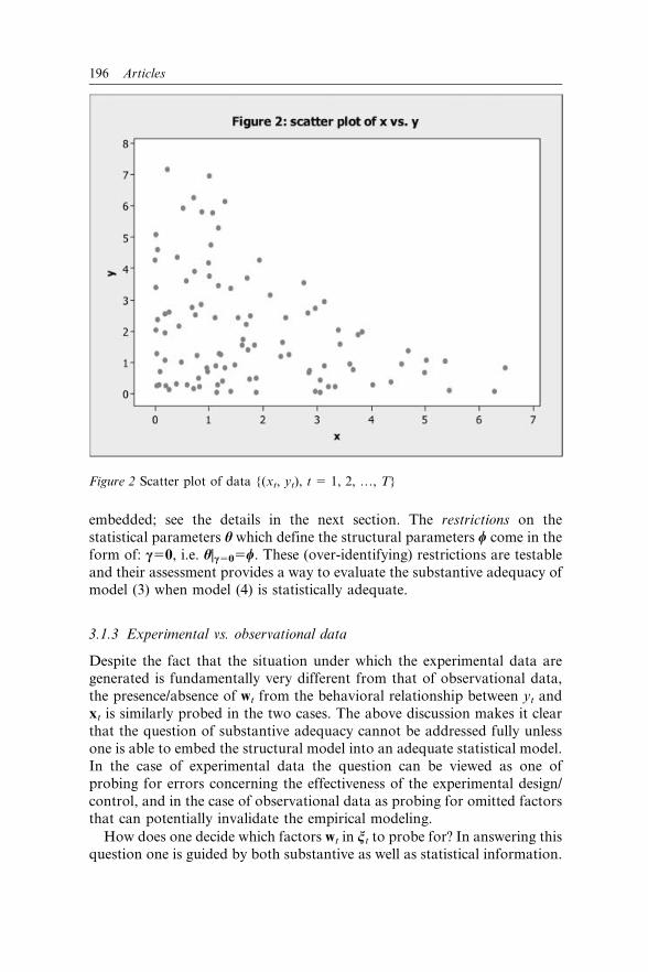
using exclusively statistical information. For instance, if the scatter plot of

the data {(xt, yt), t51, …, T} exhibits the elliptical shape shown in Figure 1,

the linearity and homoskedasticity assumptions [2]–[3] seem reasonable, but

if the data exhibit the triangular shape shown in Figure 2, then both

assumptions are likely to be false, irrespective of whether the substantive

information supports assumptions [2]–[3]. This is because the distribution

194 Articles

underlying the data in Figure 2 is bivariate exponential whose h(xk; h) is

non-linear and g(xt; h) is heteroskedastic; see Spanos (1999: ch. 6–7). In this

sense the probabilistic perspective on statistical models brings to the Table

statistical information which is distinct from the substantive information.

Indeed, the distinctness of the two types of information is at the heart of the

problem of confronting a theory with observed data enabling one to assess

its empirical validity.

An important aspect of embedding a structural into a statistical model is

to ensure that the former can be viewed as a reparameterization/restriction of

the latter. The idea is that the statistical model summarizes the statistical

information in a form which enables one to assess the substantive

information in its context. The adequacy of the structural model is then

tested against the benchmark provided by a statistically adequate model.

Often, there are more statistical parameters h than structural parameters wand the embedding enables one to test the validity of the additional (over-

identifying) restrictions w imposes on h; see Spanos (1990).

Returning to the omitted variables argument, one can view (3) as the

structural model with parameters w : ~ b, s2u

� �, and (4) as the statistical

model, with parameters h : ~ a, c, s2e

� �, in the context of which (3) is

Figure 1 Scatter plot of data {(xt, yt), t 5 1, 2, …, T}

Revisiting omitted variables 195

embedded; see the details in the next section. The restrictions on the

statistical parameters h which define the structural parameters w come in the

form of: c50, i.e. h|c505w. These (over-identifying) restrictions are testable

and their assessment provides a way to evaluate the substantive adequacy ofmodel (3) when model (4) is statistically adequate.

3.1.3 Experimental vs. observational data

Despite the fact that the situation under which the experimental data aregenerated is fundamentally very different from that of observational data,

the presence/absence of wt from the behavioral relationship between yt and

xt is similarly probed in the two cases. The above discussion makes it clear

that the question of substantive adequacy cannot be addressed fully unless

one is able to embed the structural model into an adequate statistical model.

In the case of experimental data the question can be viewed as one of

probing for errors concerning the effectiveness of the experimental design/

control, and in the case of observational data as probing for omitted factorsthat can potentially invalidate the empirical modeling.

How does one decide which factors wt in jt to probe for? In answering thisquestion one is guided by both substantive as well as statistical information.

Figure 2 Scatter plot of data {(xt, yt), t 5 1, 2, …, T}

196 Articles

The relevance of the substantive information is well understood but that ofthe statistical information is less apparent. It turns out that certain forms of

statistical misspecification in M0, which cannot be addressed using just the

statistical information in D(Z1, Z2, …, ZT; w), provide good grounds to

suspect that some key variables influencing the behavioral relationship of yt

might be missing. Hence, when repeated attempts to respecify M0 to account

for all the statistical information in D(Z1, Z2, …, ZT; w) fail, there is a good

chance that certain important factors wt in jt have been mistakenly omitted.

Moreover, the form and nature of the detected misspecification can often beof great value in guiding substantive subject matter information toward

potentially important factors.

3.2 Delineating the omitted variables argument

The textbook omitted variables argument makes perfectly good sense from the

substantive perspective in so far as one is comparing two structural explanationsfor the behavior of yt and posing a question concerning the presence of potential

confounding factors. To answer this question one needs to embed it in the

context of a coherent statistical framework. A closer look at the textbook

argument reveals that, in addition to the inadequacies raised in section 2.2, the

argument is also highly equivocal from the statistical perspective.

The above discussion of the probabilistic perspective makes it clear that

the statistical parameters are interwoven with the underlying distribution of

the observable random variables involved, and thus one needs to distinguish

between the parameters of the two models (3) and (4):

M0 : yt~x>t bzut, utjXt~xtð Þ*NIID 0, s2u

� �, t [ , ð27Þ

M1 : yt~x>t azw>t czet, etjXt~xt, Wt~wtð Þ*NIID 0, s2e

� �, t [ , ð28Þ

where, in general, by assumption: b?a and s2u=s2

e .

The statistical parameterizations associated with the two models,

w : ~ b, s2u

� �and h : ~ a, c, s2

e

� �, can be derived directly from the joint

distribution via (26), or indirectly via the error term assumptions; Spanos

(1995b). For M0 the underlying statistical parameterization is:

b~S{122 s21, s2

u~s11{s>21S{122 s21, ð29Þ

and for M1 (see Spanos, 1986: 420):

a~S{12:3 s21{S23S{1

33 s31

� �, c~S{1

3:2 s31{S32S{122 s21

� �, ð30Þ

where S2:3~S22{S23S{133 S23, S3:2~S33{S32S{1

22 S23,

s2e ~s11{ s21 s31ð Þ

S22 S23

S32 S33

� {1 s21

s31

� , ð31Þ

where s315Cov(Wt, yt), S235Cov(Xt, Wt), S335Cov(Wt).

Revisiting omitted variables 197

In view of the statistical parameterizations of the two models, the

conclusion of the textbook omitted variables argument can be stated

unequivocally as follows:

(bb, s2) in (27) are biased and inconsistent estimators of (a, s2e ) in (28).

Given that this statement is almost self-evident, the question arises, ‘how

does the equivocation affect the statistical aspects of the original argument?’

By focusing on the error terms, the textbook argument ignores the fact

that the two models, (3) and (4), have different underlying distributions;

D(yt|Xt; h) and D(yt|Xt, Wt; w), respectively. It easy to see that when E(.) and

limT??

:ð Þ are defined with respect to D(yt|Xt; h), (bb, s2) are unbiased and

consistent estimators of (b, s2u) as defined in (29). That is, when the

properties of (bb, s2) are assessed in the context of the underlying statistical

model, they are perfectly ‘good’ estimators of its parameters from the

statistical viewpoint, irrespective of whether they are substantively adequate.

Hence, statistical and substantive inadequacies raise very different issues.

By the same token, when E(.) and P limT??

are defined with respect to

D(yt|Xt, Wt; w), then the result is biased and inconsistent estimators:

EyjX, W

(bbb)~az X>X� �{1

X>Wc,yjX, W

limT??

(bbb)~azS{122 S23c, ð32Þ

EyjX, W

s2� �

~s2e z

1

T{kc>W>MXWc� �

,yjX, W

limT??

s2� �

~s2e zc>S3:2c,ð33Þ

A direct comparison between (6)–(7) and (32)–(33) indicates most clearly

that a crucial equivocation arises from the fact that the textbook omitted

variables argument in (6)–(7) does not distinguished between the implicit

parameterizations (b, s2u) and (a, s2

e ).

The question that naturally arises is whether the unambiguous results in

(32)–(33) can be used to shed light on the problem of confounding. From the

statistical perspective, the textbook omitted variables argument, restated

unequivocally in (32)–(33), has two major weaknesses:

(a) it seems to amount to a comparison between ‘apples’ (b) and

‘oranges’ (a),

(b) it offers no reliable way to evaluate the sensitivity of point

estimators.

In the next section it is argued that both of these weaknesses can be addressed

by posing the confounding question in the context of a nesting Neyman-

Pearson framework. The nesting is achieved by ensuring that the two models

(3) and (4) are based on the same statistical information, and the hypothesis

testing set up enables one to transform the bias/inconsistency terms into claims

concerning unknown parameters which can be reliably evaluated.

198 Articles

4 A TESTING PERSPECTIVE FOR OMITTED VARIABLES

4.1 Assessing substantive adequacy

In this subsection we discuss the case where the variables Wt are observed

and the relevant observable vector process is {Zt, t g } where

Zt : ~ yt, X>t , W>t

� �>. Consider two models based on the same underlying

joint distribution D(Z1, Z2, …, ZT; Q):

M0 : y~Xbzu, ujXð Þ*N 0, s2uIT

� �,

M1 : y~XazWcze, ejX, Wð Þ*N 0, s2e IT

� �:

ð34Þ

This ensures that models (M0, M1) are based on the same statistical

information, but M0 is a special case of M1 subject to the substantive

restrictions c50. In the terminology of the previous section, M0 can

be viewed as a structural model embedded into the statistical model

M1.

From this nesting perspective one can deduce, using (30)–(31), that the

parameterizations w : ~ b, s2u

� �and h : ~ a, c, s2

e

� �of the two models are

interrelated via:

a~b{Dc, c~d{Da, ð35Þ

s2e ~s2

u{ s13{s12Dð ÞS{13:2 s13{s12Dð Þ>

h i, ð36Þ

where the parameters (b, D, D, s2u) take the form:

b : ~S{122 s21, d : ~S{1

33 s31, D : ~S{122 S23, D : ~S{1

33 S32,

s2u~s11{s>21S{1

22 s21, S3:2 : ~S33{D>S23, S2:3 : ~S22{D>S32:ð37Þ

These statistical parameterizations can be used to assess the relationship

between Xt and yt by evaluating the broader issues of confounding and

spuriousness. Although these issues are directly or indirectly related to the

parameters a and b, the appraisal of the broader issues depends crucially on

the ‘true’ values of all three covariances:

s21~Cov Xt, ytð Þ, s31~Cov Wt, ytð Þ, S23~Cov Xt, Wtð Þ, ð38Þ

and in particular whether they are zero or not. In what follows it is assumed

that:

S33~Cov Wtð Þ > 0, S22~Cov Xtð Þ > 0,

in order to ensure that the encompassing model M1 is identified; see Spanos

and McGuirk (2002). It turns out that in testing the various combinations of

covariances in (38) being zero or not one needs to consider other linear

regression models directly related to the two in (34). The most interesting

Revisiting omitted variables 199

scenarios, created by allowing different combinations of covariances to be

zero, are considered below, beginning with scenarios A and B where the

parameterization of a reduces to that of b.

4.1.1 Scenario A: s3150 and S2350, given s21?0 (no confounding)

Under these covariance restrictions, the parameters h : ~ a, c, s2e

� �take the

form:

ajS32~0s31~0

~S{122 s21~b, cjS32~0

s31~0

~0, s2e

��S32~0

s31~0

~s11{s>21S{122 s21~s2

u: ð39Þ

In scenario A model M1 reduces to model M0.

The ‘given’ restrictions s21?0 should be tested first using an F-test (see

Spanos 1986: 399) for the hypotheses:

M0ð Þ H0 : b~0 vs: H1 : b=0, ð40Þ

where (M0) indicates that the testing takes place in the context of

M0. Assuming that H0 was rejected, one can proceed to test s3150 and

S2350.

The restriction s31?0 can be similarly tested using the hypotheses:

M2ð Þ H0 : d~0 vs: H1 : d=0: ð41Þ

in the context of the linear regression:

M2 : y~Wdzv, vjWð Þ*N 0, s2vIT

� �, ð42Þ

s2v~s11{s>31S{1

33 s31. In view of the fact that D : ~S{122 S23, the restriction

S2350 can be tested using the hypotheses:

M3ð Þ H0 : D~0, vs: H1 : D=0, ð43Þ

in the context of the multivariate linear regression:

M3 : W~XDzU2, ð44Þ

(see Spanos, 1986: ch. 24). It is important to note that the bias/inconsistency

term for bbb in (32) has been transformed into the hypotheses (43), since

bDD~ X>X� �{1

X>W� �

. The appropriate test for (43) is a multivariate F-type

test (see Spanos 1986: 593–5), which is more difficult to apply than the F-

tests for (40) and (41).

Searching for a simpler way to test the restrictions (S2350, s3150), we

note that in view of (30), (S2350 and s3150) imply c50 (given s21?0), and

thus they can can be tested using:

M1ð Þ H0 : c~0 vs: H1 : c=0: ð45Þ

200 Articles

The F-test for (45) takes the form (see ibid.: 399–402):

F yð Þ~ buu>buu{bee>beeð Þbee>bee

T{k{m

m

� *F d; m, T{k{mð Þ,

C1~ y : F yð Þ > caf g being the rejection region,

ð46Þ

where T is the number of observations; k, the number of included variables;

m, the number of omitted variables; buu~y{Xbbb, bee~y{Xbaa{Wbcc, the

residuals from the two models; d~c>W>MX Wcð Þ

s2e

, the non-centrality para-

meter. The form of the F-test is particularly interesting in this case because

the recasting of the confounding question in a testing framework has

transformed the estimation bias of s2 in (33) into d which determines the F-

test’s capacity (power) to detect discrepancies from the null, when present.

It is interesting to note that testing (45) is directly related to the testing of

the conditional independence assumption in the context of graphical causal

modeling, associated with Spirtes et al. (2000) and Pearl (2000); see Hoover

(2001). That is, the F-test for (45) provides an effective way to test the

hypothesis that yt conditional on Xt is independent of Wt. At the same time

the above discussion brings out the possibility of highly unreliable inferences

when one focuses exclusively on the conditional independence restriction

c50, ignoring the covariances (s21, s31, S23). Indeed, a question that

naturally arises at this stage is whether testing (45) is equivalent to testing

(41) and (43) simultaneously. It turns out that equivalence holds only if one

excludes the possibility that d5Da; see (35). This possibility arises when the

null in (45) is rejected because S23?0 and s31?0 hold. This case is excluded

by the so-called faithfulness assumption invoked in graphical causal modeling;

see Spirtes et al. (2000) and Pearl (2000). As argued below under scenario F,

however, there is no need to impose the faithfulness assumption a priori

because in that scenario the restrictions d5Da turn out to be testable.

Acceptance. In the case where the null hypotheses in (41) and (43) are

accepted, but the null in (40) is rejected, one can infer (under certain

circumstances, to be discussed in section 4.2) that the Wt variables do not

confound the effect of Xt on yt. These circumstances concern primarily the

question of substantive vs. statistical insignificance, which need to be

investigated further using Mayo’s (1991) post-data evaluation of inference

based on severe testing. Accepting the null hypotheses in (41) and (43)

establishes statistically insignificance, but the question of substantive

insignificance (no confounding) needs to be investigated further; it could

be the case that the test applied had no power to detect discrepancies of

substantive interest. In the case where substantive insignificance can be

established (see section 4.2), one can deduce that the estimated model M0

will give rise to more precise inferences than model M1 because:

Cov baað Þ{Cov(bbb)§0.

Revisiting omitted variables 201

Rejection. The case where all null hypotheses in (41), (43) and (40) are

rejected, gives rise to scenario F to be discussed below. The case where the

null hypotheses in (41) and (43) are rejected, but the null in (40) is accepted,

gives rise to scenario D.

4.1.2 Scenario B: S2350, given s31?0, s21?0 (no confounding)

Under these covariance restrictions, the parameters h : ~ a, c, s2e

� �take the

form:

ajS32~0~S{1

22 s21~b, cjS32~0~S{133 s31~d,

s2e

��S32~0

~s2u{s13S{1

33 s>13~s23:

ð47Þ

In scenario B, M1 reduces to:

M13 : y~XbzWdze3, e3jX, Wð Þ*N 0, s23IT

� �, ð48Þ

where the parameters b and d coincide with the regression coefficients in

models M0 and M2, respectively; note, however, that s23=s2

e=s2u=s2

v .

The ‘given’ restrictions s21?0, s31?0, should be established first by

testing them in the context of models M0 and M3, respectively using (40)

and (41). Assuming that both null hypotheses in (40) and (41) have been

rejected, one can proceed to test S2350 in the context of model M2 using

(43).

Acceptance. When the null hypothesis in (43) is accepted and those in (40)

and (41) are rejected, one can infer (under certain circumstances, to be

discussed in section 4.2) that aa in model M1 constitutes a ‘good’ estimator of

b~S{122 s21 in model M0, i.e., the omitted variables Wt do not confound the

effect of Xt on yt, even though Wt is relevant in explaining yt. More

generally, the effect of Xt on yt can be reliably estimated when one can

establish the non-correlation between the included (Xt) and omitted (Wt)

variables. It is important to emphasize that this result is confined to the

point estimation and does not extend to the reliability of other forms of

inference concerning b, such as confidence-intervals and hypothesis testing

because the latter require a consistent estimator of s23.

Rejection. The case where all the null hypotheses in (43), (40) and (41) are

rejected, gives rise to scenario F below. In the context of the latter scenario

one can infer that the omitted variables Wt are likely to confound the effect

of Xt on yt, but the extent of the confounding needs to be investigated

further using severe testing; see section 4.2. The case where the null

hypothesis in (43) is rejected, and those in (40) and (41) are accepted, gives

rise to a scenario G (s2150, s3150, S32?0). This and scenario H (s2150,

s3150, S3250) are uninteresting from our perspective because neither set of

variables Xt or Wt is relevant in explaining yt.

202 Articles

4.1.3 Scenario C: s3150, given s21?0, S32?0 (‘apparent’ confounding)

Under these covariance restrictions, the parameters h : ~ a, c, s2e

� �take the

form:

ajs31~0~S{12:3 s21~a1, cjs31~0~{S{1

3:2 S32S{122 s21~{Da1~c1,

s2e

��s31~0

~s11{s>21 S{122 {DS{1

3:2 D>� �

s21~s21,

ð49Þ

In scenario C model M1 reduces to:

M11 : y~Xa1zWc1ze1, e1jX, Wð Þ*N 0, s21IT

� �: ð50Þ

The ‘given’ restrictions s21?0 and S32?0 can be tested in the context of

models M3 and M0, respectively, using (40) and (43). Assuming that the null

hypotheses in (43) and (40) have been rejected, one can proceed to test

s3150 using (41) in the context of model M3 to establish scenario C.

Similarly to scenario A, searching for a more convenient way to test these

restrictions, one can see that in view of (30), (S2350 and s2150) imply a50

(given s31?0 - see scenario E), and thus one can test both coefficient

restrictions simultaneously using the F-test for the hypotheses:

M1ð Þ H0 : a~0 vs: H1 : a=0, ð51Þ

whose form is analogous to that in (46). This test is equivalent to testing (41)

and (43) simultaneously only if one were to exclude the possibility that

b5Dc; this case arises from rejecting the null in (35) when S23?0 and s21?0

hold. In graphical causal modeling this equivalence holds because this case is

excluded by the faithfulness assumption; see Spirtes et al. (2000). When

s21?0, s31?0, S23?0 scenario F holds, and the restrictions b5Dc turn out

to be testable in its context.

It is instructive to consider an alternative (but related) way to assess the

validity of the hypotheses in (41) arising from the fact that when the

restrictions c152Da1 are imposed on M11 it reduces to y5[X2WD]a1+e1.

Hence, an estimation-based sensitivity assessment of the validity of (41) can

be based on comparing the estimates of a1 in (50) with those of a�1 from the

restricted model:

M�11 : y~bUU1a�1ze�1, bUU1~X{WbDD, ð52Þ

where bDD~ W>W� �{1

W>X, and bUU1 denotes the matrix of the residuals from

the multivariate regression:

M4 : X~WDzU1: ð53Þ

The comparison of the two estimators baa1 (based on M11) and baa�1 (based on

M�11) will involve, not only the estimates but also their standard errors, as

well as the standard errors of the two regressions, restricted and

unrestricted. This estimation-based evaluation differs crucially from the

Revisiting omitted variables 203

textbook omitted variables argument, based on the difference (bbb{baa) in (8),

in so far as baa1 and baa�1 are estimating the same parameter a1. In this sense,

(baa1{baa�1) provides a more appropriate basis for assessing the sensitivity of

these estimates than (bbb{baa). Indeed, the difference (baa1{baa�1) is directly

related to the F-test based on the difference between restricted and

unrestricted residual sums of squares arising from the two models.

Acceptance. When the null hypothesis in (41) is accepted, but those in (40)

and (43) are rejected, one can infer (under certain circumstances - see

section 4.2) that the textbook omitted variables argument based on the

difference (bbb{ebb) in (8) will be very misleading because it will (erroneously)

indicate the presence of confounding. This is because (bbb{ebb) is likely to be

sizeable, reflecting b{a1ð Þ~ S{122 {S{1

2:3

� �s21=0, but in reality Wt has no

role to play in establishing the ‘true’ relationship between Xt and yt since

Cov(Wt, yt)50.

Rejection. The case where all null hypotheses in (41), (40) and (43) are

rejected gives rise to scenario F (see below), which, in turn calls for further

probing in order to establish the extent of the confounding effect using

severe testing (see section 4.2). The case where the null hypothesis in (41) is

rejected, but those in (40) and (43) are accepted, gives rise to scenario E

below.

4.1.4 Scenario D: s2150 given S32?0, s31?0 (spurious)

Under these covariance restrictions, the parameters h : ~ a, c, s2e

� �take the

form:

ajs21~0~{S{12:3 S23S{1

33 s31~{Dc2~a2, cjs21~0~S{13:2 s31~c2,

s2e

��s21~0

~s11{s13S{13:2 s>13~s2

2:ð54Þ

In scenario D model M1 reduces to:

M12 : y~Xa2zWc2ze2, e2jX, Wð Þ*N 0, s22IT

� �: ð55Þ

The ‘given’ restrictions S32?0, s31?0 should be tested first in the context of

M3 and M2, respectively. Assuming that the null hypotheses in (43) and (41)

are rejected, one can proceed to test the restrictions s2150 in the context of

model M0 using (40).

In direct analogy to scenario C, an alternative (but related) way to assess

the validity of the hypotheses in (40) be based on imposing the restrictions

a252Dc2, which will reduce M12 to y5[W2XD]c2+e2. Hence, an estimation-

based sensitivity assessment of the validity of (40) can be performed by

comparing the estimates of c2 in (55) with those from the restricted model:

M�12 : y~bUU2c2ze�2, bUU2~W{XbDD, ð56Þ

204 Articles

where bDD~ X>X� �{1

X>W and bUU2 denotes the matrix of the residuals from

the multivariate regression (44).

Acceptance. When the null hypothesis in (40) is accepted but those in (41)

and (43) are rejected, one can infer (under certain circumstances, to be

discussed in section 4.2) that the relationship between Xt and yt in M0 is

spurious. Moreover, the textbook omitted variables argument based on the

difference (bb{aa) in (8) can be misleading. This is because the difference

(bb{aa) will reflect b{a2ð Þ~{S{12:3 S23S{1

33 s31=0, which should not be

interpreted as indicating the presence of confounding, but the result of a

spurious relationship between Xt and yt.

Rejection. The case where all null hypotheses in (40), (41) and (43) are

rejected gives rise to scenario F discussed below. The case where the null

hypothesis in (40) is rejected but those in (41) and (43) are accepted, gives

rise to scenario A above.

4.1.5 Scenario E: S2350, s2150, given s31?0 (spurious)

Under these covariance restrictions, the parameters h : ~ a, c, s2e

� �take the

form:

ajS32~0s21~0

~0, cjS32~0s21~0

~S{133 s31~d, s2

e

��S32~0s21~0

~s11{s13S{133 s>13~s2

v : ð57Þ

In scenario E model M1 reduces to:

M2 : y~Wdzv, vjWð Þ*N 0, s2vIT

� �: ð58Þ

The ‘given’ restrictions s31?0 can be tested in the context of model M2 using

(41); see scenario B. Assuming the null hypothesis in (41) has been rejected,

one can proceed to test the restrictions S2350, s2150 in the context of

models M3 and M0, respectively, using (43) and (40). As argued above, (57)

suggests that (S2350, s2150) implies a50, and if one were to exclude the

possibility that b5Dc (see scenario F), testing (S2350, s2150) is equivalent

to using the F-test for the hypotheses (51) in the context of M1; see scenario

C. Note that under scenario D, M1 reduces to M2 in (42).

Acceptance. When the null hypotheses in (43) and (40) are accepted, and

the null in (41) is rejected, one can infer (under certain circumstances, to be

discussed in section 4.2) that the relationship between Xt and yt in M0 is

spurious. Moreover, the textbook omitted variables argument based on the

difference (bb{aa) in (8) can be misleading. This is because (bb{aa) will reflect

b{a2ð Þ~S{133 s31=0, which should not be interpreted as indicating the

presence of confounding, but as a result of a spurious relationship between

Xt and yt.

Rejection. The case where all null hypotheses in (43), (40) and (41) are

rejected, gives rise to scenario F, discussed next. The case where the null

Revisiting omitted variables 205

hypotheses in (43) and (40) are rejected but the null in (41) is accepted, gives

rise to scenario C above.

4.1.6 Scenario F: S23?0, s31?0, s21?0 (possible confounding)

Under these covariance restrictions model M1 in (34) remains unchanged

and the parameters h : ~ a, c, s2e

� �take the original form given in (35)–(36).

This raises the possibility of confounding but the extent of the effect needs

to be quantified. In this scenario one needs to establish that all three

covariances (S23, s31, s21) are non-zero by testing them separately in their

respective statistical models M3, M2 and M0 by rejecting the null

hypotheses. Let us assume that S23?0, s31?0, s21?0 have been established.

Does that mean that there is confounding? Not necessarily, because the null

the hypothesis in:

M1ð Þ H0 : c~0 vs: H1 : c=0, ð59Þ

can still be true in the case where (see (35)):

d~Da, ð60Þ

(assuming that a?0) because, in view of (35), (60) implies c50. As

mentioned above, in the graphical causal modeling literature the restrictions

(60) are ruled out by the assumption of the causal faithfulness; see Spirtes et

al. (2000) and Pearl (2000). The above discussion, however, indicates most

clearly that one need not impose the causal faithfulness assumption a priori

because the implicit restrictions are testable in this context of scenario F.

That is, given S23?0, s31?0, s21?0, this assumption becomes testable via

(59). When the null hypothesis c50 is accepted the restrictions excluded by

the faithfulness assumption do, in fact, hold. When the null hypothesis c50

is rejected, one can proceed to quantify the extent of the confounding effect,

using the results of the next subsection.

Similarly, the restrictions S23?0, s31?0, s21?0 do not necessarily imply

that a?0. It follows from (35) that in scenario F a50 when the restrictions

(see (35)):

b~Dc, ð61Þ

excluded by faithfulness, hold; assuming that c?0.

In concluding this subsection, it is important to re-iterate that the above

discussion of the Neyman-Pearson (N–P) testing revolving around scenarios

A–F has been heavily qualified. The assessment of confounding

and spuriousness needs to go beyond the traditional N–P testing ‘accept/

reject’ decisions, and consider the question of whether such deci-

sions provide evidence for the hypothesis that ‘passed’, which we consider

next.

206 Articles

4.2 Severe testing: assessing substantive significance

The testing results of the previous subsection have been heavily qualified

because the Neyman-Pearson testing procedure, based on the coarse ‘accept/

reject’ rules, is susceptible to both the fallacy of acceptance (interpreting

‘accept H0’ as evidence for a substantive claim associated with H0), and the

fallacy of rejection (interpreting ‘reject H0’ as evidence for a substantiveclaim associated with H1). In order to address these fallacies Mayo (1991,

1996) proposed a post-data assessment of the Neyman-Pearson ‘accept/

reject’ decisions based on evaluating the severity with which a claim passes

the particular test with data z0. In particular, the severe testing reasoning

can be used to assess the substantive significance of claims discussed in

relation to the confounding problem. This post-data evaluation, based on

severe testing, supplements the Neyman-Pearson decision rules with an

evidential interpretation that renders the inference considerably moreinformative by distinguishing clearly the claims that are or are not

warranted on the basis of the particular data; see Mayo and Spanos

(2006) for further details.

A hypothesis H (H0 or H1) passes a severe test t(Z) with data z0 if,

N (S-1) z0 agrees with H, and

N (S-2) with very high probability, test t(Z) would have produced a

result that accords less well with H than z0 does, if H were false.

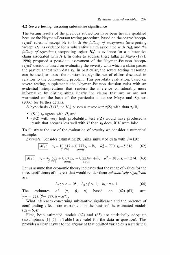
To illustrate the use of the evaluation of severity we consider a numerical

example.

Example. Consider estimating (9) using simulated data with T5120:

M0 : yt~ 10:6175:497ð Þ

z 0:777xt0:039ð Þ

zbuut, R20~:770, su~5:816, ð62Þ

M1 : yt~ 48:5628:896ð Þ

z 0:671xt0:041ð Þ

{ 0:223wt0:043ð Þ

zbeet, R21~:813, se~5:274: ð63Þ

Let us assume that economic theory indicates that the range of values for the

three coefficients of interest that would render them substantively significant

are:

hc : cv{:05, hb : bw:1, ha : aw:1 ð64Þ

The estimates of (c, b, a) based on (62)–(63), are:

bcc~{:223, bbb~:777, baa~:671.

What inferences concerning substantive significance and the presence of

confounding effects are warranted on the basis of the estimated models

(62)–(63)?

First, both estimated models (62) and (63) are statistically adequate

(assumptions [1]–[5] in Table 1 are valid for the data in question). Thisprovides a clear answer to the argument that omitted variables is a statistical

Revisiting omitted variables 207

misspecification issue; both models can be statistically but not substantively

adequate. Having established statistical adequacy one can proceed to

compare the two models on other grounds, including goodness of fit and

substantive adequacy. For example, M1 is clearly better on goodness of fit

grounds since R21 > R2

0, but is it better on substantive grounds? To establish

that one needs to assess the claims in (64) using Neyman-Pearson testing,

supplemented with a post-data evaluation of inference based on the notion

of severe testing; see Mayo (1996).

Testing the hypotheses:

M1ð Þ H0 : c~0, vs: H1 : cv0, ð65Þ

using a t-test based on tc Zð Þ~ bcc{0

dSE bcc� �

SE bcc� �, with a rejection region

C15{z:tc(z),ca}, yields tc z0ð Þ~ {0:2230:043

~{5:186 :000005½ �. The p-value (in

square brackets) indicates a rejection of H0:c50. In relation to severity,

condition (S-1) the p-value indicates that z0 agrees with H1. This suggests

that c is statistically different from zero for some discrepancy c1,0, but does

not establish the size c1 of the warranted discrepancy. When the null is

rejected, the goal is to be able to license as large a discrepancy c1 from the

null as possible. Severity reasoning establishes the warranted discrepancies

by evaluating the probability that ‘test tc(Z) would have produced a result

that accords less well with H1 than z0 does, if H1 were false’, i.e.

SEV tc z0ð Þ; cvc1

� �~ tc Zð Þwtc z0ð Þ; cvc1 is false

� �

~ tc Zð Þwtc z0ð Þ; c§c1

� �:

Choosing different values for c1 one can show1 that:

which suggest that the severity of inferring c,c1, for 2.150,c1,0, with

test tc(Z) and data z0, is very high, i.e. the claim is warranted. Moreover, the

severity of inferring the substantive claim hc:c,2.05 in (64) is 1, on the basis

of which one can infer the substantive significance of c. That is, the test

value tc(z0)525.186[.000005] establishes the statistical significance of c, and

the severity evaluation in Table 4 establishes its substantive significance in

relation to (64).

Having established the substantive significance of the coefficient of Wt,

we can now proceed to consider the question whether Wt confounds the

effect of Xt on yt. The null hypothesis of interest:

M0ð Þ H0 : b~0, vs: H1 : b > 0, ð66Þ

Table 4 Severity Evaluations for c,c1

c1 2.050 2.100 2.150 2.200 2.300SEV(tc(z0); c,c1) 1.000 .997 .954 .703 .038

208 Articles

is rejected on the basis of the t-test: tb Zð Þ~ bbb{0

dSE bbb� �

SE bbb� �, C15{z:tb(z).ca}, since it

yields tb z0ð Þ~ :777:039

~19:923 :000000½ �. The severity evaluation for the claim

b.b1, for some b1.0, takes the form (see Mayo and Spanos 2006):

SEV tb z0ð Þ; b > b1

� �~ tb Zð Þƒtb z0ð Þ; b > b1 is false

� �

~ tb Zð Þƒtb z0ð Þ; bƒb1

� �,

ð67Þ

giving rise to the following error probabilistic assessments2:

In view of hb:b..1 in (64) one can argue that the claim b.b1 with b1(.7

passes severely with data z and the above t-test, and that establishes the

substantive significance of b.

Applying the same t-test to the hypotheses:

M1ð Þ H0 : a~0, vs: H1 : a > 0, ð68Þ

yields ta z0ð Þ~ :671:041

~16:366 :000000½ �, which also rejects H0. The same

severity evaluations as in (67) for the claim a.a1 give rise to:

On the basis of the evaluations in Table 5, the claim a..6, is warranted

with test tc(Z) and data z0. Moreover, the severity for inferring the

substantive claim ha:a..1 in (64) is 1, on the basis of which one can infer the

substantive significance of a.

Using the evaluations of severity in Tables 5–6, one can make a case that

there is a deviation between the warranted discrepancies associated with

rejecting the null in the case of the hypotheses (66) and (68). By choosing a

high enough severity threshold, say .975, one can argue that the warranted

discrepancy from b50, associated with the claim b.b1 is b15.700, but that

from a50, associated with the claim a.a1 is a15.590. An informal

comparison between the two claims (ad hoc t-test) indicates that the

difference (b12a1)5.110 is likely to be statistically different from zero, and

the severity evaluations in Tables 5–6 suggest that it’s also likely to be

substantively significant. A more formal assessment of these claims can be

based on (b2a)5(b12a1)?0, but the resulting test is rather involved

because it requires reparameterizing M1.

Table 5 Severity Evaluations For b.b1

b1 .600 .650 .700 .750SEV(tb(z0); b.b1) 1.00 .999 .975 .755

Table 6 Severity Evaluations For a.a1

a1 .500 .550 .590 .600 .650SEV(ta(z0); a.a1) 1.00 .998 .975 .957 .695

Revisiting omitted variables 209

The above severity evaluations provide support for scenario F: s21?0,

s31?0, s32?0. The estimated models M0 and M1 in (62)–(63) provide

evidence that when Wt is omitted (a) the effect of Xt on yt is over-estimated,and (b) the structural model M0 is substantively inadequate.

4.2.1 The severe testing reasoning vs. other tail area evaluations

In concluding this subsection, it is important to emphasize that severe

testing, puts forward a post-data evaluation of a specific claim in accordance

with the null or the alternative hypotheses decided on the basis of a specific

Neyman-Pearson test result. In this sense the underlying reasoning isdifferent from that implicit in other error probabilities such as type I and II

error probabilities, power, confidence level and p-values. In view of the fact

that all these error probabilities are based on the evaluation of tail areas of

the same sampling distributions (t-tests in this case), there is always some

algebraic relationship that enables one to relate, in some ad hoc way, all

these error probabilities. However, it is a mistake to confuse these ad hoc

relationships with the different rationales underlying the various error

probabilities.What is important is the underlying reasoning that enables one to assess

claims concerning the parameters of interest on the basis of the data. It is

well-known that the type I and II (or power) error probabilities are pre-data

error probabilities based on a predesignated rejection value ca, determined

by the chosen significance level a. As shown above, the severity evaluation is

based on the observed value of the test statistic t(z0) and not ca. Moreover, it

is well known that no error probability can be attached to observed

confidence-intervals, say (.699(b,.855); see Cox and Hinkley (1974).Hence, the probabilistic reasoning associated with the severity evaluation is

very different from that of confidence-interval estimation, which revolves

around defining a random interval that would cover the ‘true’ value of the

parameter h (whatever that happens to be) with a predesignated probability

(12a). This does not preclude the existence of some relationship between

(12a) and the severity evaluation since, as mentioned above, they are both

based on the same sampling distribution. Similarly, the severe testing

reasoning is different from the p-value rationale, even though one canalways find an algebraic relationship between the two tail areas; see Mayo

(1996), Mayo and Spanos (2006) for further details.

4.3 Unobserved omitted variables

Consider the case where no data on the potentially crucial factors Wt are

available. In such a case one might still be able to assess whether bb might

provide an underestimation/overestimation of a using certain qualitativeinformation. To that end, the relationship between the parameterizations of

210 Articles

b and a (see (35)):

b~azS{122 S23c, ð69Þ

provides the most promising way to shed light on the issue. Assuming that

one has some qualitative information concerning the sign and approximate

magnitudes of (S23, c), one can put forward a qualitative assessment

argument concerning the potential inaccuracies of bbb as an estimator of a.

For example, in the case where Wt comprises a single factor Wt, and there is

qualitative information that S23.0, c.0, then one can deduce that bbb is

likely to underestimate a. Similarly, when:

S23.0, c,0, bb is likely to overestimate a;

see Stock and Watson (2002: 146).

A closer look at this qualitative assessment argument, however, reveals that

it needs to be qualified. As argued above, appraising the sign and magnitude

of a coefficient could not rely exclusively on the value of an estimate, but

should also take account for the relevant standard error derived from

Cov baað Þ~s2e X>PWX� �{1

, where PW5W(WiW)21Wi, which includes the

conditional variance as given in (36), i.e., the coefficient can be

insignificantly different from zero. A glance at these formulae suggests that

it will be a non-trivial matter to assess that. Hence, even for the simp-

lest cases where there is only one missing factor, the assessment based

on how bb is likely to underestimate/overestimate a can easily lead one

astray.

A clearer qualitative assessment is possible when there is qualitative

information that strongly indicates Cov(Xt, Wt)50. In that case, the

estimator bb based on (27) will provide a reliable point estimator of the effect

of Xt on yt, even when Wt is substantively significant in explaining yt.

4.4 Omitted variables and misspecification testing

An interesting variation on the testing framework created by the two nested

models (27) and (28) in sections 4.1–4.2 arises when Wt does not represent

additional variables, but functions of the original variables (yt, Xt) such as

higher powers of the xit’s, say their second order functions yt:5(xit?xjt)i,j, i,

j52, …, k, lags zt2i:5(yt2i, xt2i), i51, 2, …, ,, and trends t:5(t, t2, .., tm).

The discussion above can be adapted to provide a general framework for

constructing misspecification tests based on artificial regressions; see Spanos

(2005b) for more details.

For instance, one can construct a misspecification test for departures

from the linearity assumption [2] (see table 1) by using

E ytjXt~xtð Þ~a0za>1 xtza>2 yt, as an approximation to a non-linear

Revisiting omitted variables 211

regression function. The two regression functions give rise to two competing

models:

M0 : yt~b0zb>1 xtzut, M1 : yt~a0za>1 xtza>2 ytzet, ð70Þ

which are comparable because they share the same statistical information

based on D(Z1, …, ZT; Q), where Zt:5(yt, Xt). A comparison between them

(subtracting M0 from M1) gives rise to the artificial regression:

ut~ a0{b0ð Þz a>1 {b>1� �

xtza>2 ytzet, ð71Þ

or equivalently, its operational form:

buut~(a0{bbb0)z a>1 {b>1� �

xtza>2 ytzet, ð72Þ

based on the estimated M0. (72) provides the basis for a misspecification test

for the linearity assumption [2] using the hypotheses:

M1ð Þ H0 : a2~0 vs: H1 : a2=0: ð73Þ

The set-up in (70) can be easily extended to derive misspecification tests for

the other assumptions using artificial regressions, as well as joint

misspecification tests for assessing the validity of several assumptions

simultaneously; see Spanos (2005b) for further details.

In concluding this subsection it is interesting to mention that an early

attempt to use the omitted variables argument as a basis for constructing

misspecification tests was Pagan (1984), whose use of the equivocal notation

in (3)–(4) gave rise to the inappropriate artificial regression u5Wc+e. The

difference in the two parameterizations in M0 and M1 gives rise to the

additional terms (a02b0) and a>1 {b>1� �

xt which contribute significantly to

the power of the misspecification test based on (73); see Spanos (2005b).

4.5 Omitted variables as instruments

Another interesting variation on the two nested models (27) and (28) in

section 4.1 arises when (27) is a structural model of the form:

M�0 : yt~X>t dzvt, vtjWt~wtð Þ*NIID 0, s2

v

� �, t [ , ð74Þ

where (i) E(Xtvt)?0, and Wt represents a m61 (m>k) vector of instrumental

variables such that:

iið Þ E Wtvtð Þ~0, iiið Þ Cov Xt, Wtð Þ~S23=0,

ivð Þ Cov Wtð Þ~S33 > 0, vð Þ Cov yt, Wtð Þ~s13=0:

This model is widely used in econometric modeling because it encompasses

the case of a single equation from a Simultaneous Equations Model. The

moment restrictions (ii)–(v) define Wt as correlated with yt, but yt and Wt

are conditionally uncorrelated given Xt; see Spanos (2006b). Hence, Wt can

212 Articles

be viewed as a set of (legitimately) omitted variables which can be used as

instruments for estimating the structural parameters (d, s2v). As shown in

Spanos (1986), the statistical model in the context of which the structural

model (74) is embedded is not (28), but the implicit reduced form:

M�1 : yt~w>t b1zu1t, Xt~w>t B2zu2t,

u1tjWt~wtð Þ

u2tjWt~wtð Þ

!

*NIID0

0

!

,v11 v12

v21 V22

! !

:ð75Þ

This statistical model, based on D(yt, Xt|wt; y) is related to (28), based on

D(yt|Xt, wt; Q1), via:

D yt, Xtjwt; yð Þ~D ytjXt, wt; Q1ð Þ:D Xtjwt; Q2

� �, ð76Þ

giving rise to the reparameterized statistical model:

M�2 : yt~X>t azw>t czet, Xt~w>t B2zu2t,

etjXt, Wt~wtð Þ

u2tjWt~wtð Þ

!

*NIID0

0

!

,s2

e 0

0 V22

! !

, t [ :ð77Þ

In contrast to scenarios A (c50) and B (S2350) of the previous section, the

restrictions imposed on (77) are:

M�2

� �c~0, subject to b1=0, B2=0: ð78Þ

That is, the implicit structural parameterization (d, s2v) in (74) takes the

form:

aj c~0, b1=0 B2=0½ �~d~ S23S{133 S23

� �{1S23S{1

33 s31,

s2e

��c~0, b1=0 B2=0½ �~s2

v~s11{s12 S23S{133 S23

� �{1S23S{1

33 s31:ð79Þ

This shows most clearly that d in (74) and the parameters b and a in (34) can

represent very different effects of Xt on yt; Spanos (1986, 2006).

Noting that c5b12B2a, one can see that the restrictions (78) amount to

(m2k) restrictions on (b1, B2) that transform the statistical parameter a into

the structural parameter d. These are the so-called over-identifying

restrictions which are testable, but the reliability of such a test depends

crucially on the statistical adequacy of the statistical model (75). Indeed, the

choice of ‘optimal’ instruments is depends crucially on the statistical

adequacy of (75). For instance, if the vector stochastic process {Zt, t g },

where Zt : ~ yt, X>t , W>t

� �>, is Markov dependent (see Spanos 1999: ch. 8),

the set of optimal instruments that would render (75) statistically adequate is

likely to include lags of this process, even if the relevant static economic

theory might suggest that the past history of the process is irrelevant; see

Spanos (1986: ch. 25). It is important to emphasize that the restrictions

Revisiting omitted variables 213

b1?0, B2?0 are testable, and need to be tested, in the context of the

statistical model (75) before testing the overidentifying restrictions.

If we return to the original question of substantive adequacy, as it relates

to (78), we can see that the numerical difference between the values of the

two least-squares estimators:

bdd~ X>X� �{1

X>y, baa~ X>MW X� �{1

X>MW y,

where MW5I2W(WiW)21Wi, provide no valuable information concern-

ing the sensitivity of this inference. This is because this difference has no

direct bearing on the substantive hypotheses (78). What might be more

informative in this case is the difference between the OLS and the

Instrumental Variables estimators:

bddIV ~ X>PW X� �{1

X>PW y, where PW ~I{MW :

Indeed, the difference (bdd{bddIV ), which is related to (78), provides the basis of

the Durbin-Wu-Hausman test for exogeneity; see Spanos (2006c) for further

details.

An important conclusion following from the above discussion is that the

numerical similarity between two Instrumental Variables estimators of d,

based on two different sets of instruments, say W1t and W2t, does not

indicate the appropriateness of either set of instruments; they can both lead

to equally unreliable inferences. What establishes appropriateness and

inappropriateness in this context is the statistical adequacy of the

embedding statistical model (75) and the substantive adequacy of the

structural model in question, not the apparent numerical insensitivity of

the estimates to the choice of instruments.

5 STATISTICAL INADEQUACY AND SUBSTANTIVE

INFERENCE

Throughout the discussion of assessing substantive adequacy in sections 2–

4, it was assumed that both models M0 (27) and M1 (28) were statistically

adequate; assumptions [1]–[5] (see Table 1) are valid for M0 (with Xt) and M1

(with X�t : ~ X t, W tð Þ). When this is not the case, the discrepancy between

nominal and actual error probabilities will often give rise to unreliable

inferences; see Spanos (2005a).

Setting 1: Models M0 and M1 are both statistically adequate. This is the

case where we know that both sets of parameters (b, s2u) and (a, c, s2

e ) will be

statistically well estimated, and any tests will have the correct size and power

characteristics; the discussion concerning scenarios A–E in section 4.1, go

through unaltered.

Setting 2: M1 is statistically adequate but M0 is statistically inadequate. In

this case the discussion concerning scenarios A–E needs to be qualified. Any

214 Articles

tests of hypotheses concerning b in the context of model M0 are likely to be

affected by its statistical inadequacy. However, the F-test for hypotheses in

the context of M1 is robust to the statistical inadequacy of M0 because, in

the case of testing the restrictions c50, it coincides with the Wald (W) test

which is based exclusively on the estimators of M1. In particular, one can

show that the F-test statistic in (46), reduces to:

F yð Þ~Rbdd� �>

R X�>X�ð Þ{1R>

h i{1

Rbdd� �

ms2e

~W yð Þ, ð80Þ

where R~ 0m|k : Im|mð Þ, bdd~ baa>, bcc>ð Þ>, X� : ~ X : Wð Þ, s2e ~ bee>bee=T{k{mð Þ.

Given that M1 is statistically adequate, the actual power properties of both

tests will coincide with the nominal, but the nominal type I error

probabilities might differ from the actual ones because the latter are

evaluated under M0; this is less of a problem for testing S2350 because the

relevant statistical model under this restriction remains M1.

The danger with this case is that when one does not do a sufficiently

competent job in respecifying the original model with the view to reach a

statistically adequate model using data {(Wt, yt) t51, 2, …, T}, the presence

of departures from the probabilistic assumptions might be erroneously

interpreted as an indication of missing factors. Such a misleading inference

is likely to be confirmed when such omitted variables are included in the

model because, more often than not, Wt can play the role of a ‘proxy’ for

certain missing statistical information such as trends, temporal dependence

and non-linearities, irrespective of their substantive significance. This

problematic situation can be prevented by establishing the statistical

adequacy of M1 itself, and not relying on the statistical inadequacy of M0

as providing evidence for M1.

Setting 3: M1 is statistically inadequate but M0 is statistically adequate. In

this case the testing procedure concerning scenarios A–E need to be

modified. Given that M0 is statistically adequate, the type I error probability

of the test for c50 will coincide with the actual, but its nominal power is

likely to differ from the actual. Hence, in testing a50 or c50, one might

supplement the F-test with the Lagrange Multiplier (LM) test, which is less

vulnerable to the statistical inadequacy of M1, because it is based exclusively

on the estimators of M0. In particular, one can show that the LM test (see

Spanos, 1986, ch. 20) takes the form:

LM yð Þ~y{Xbbb� �>

W W>MX W� �{1

W>h i

y{Xbbb� �

ms2u

*F d�; m, T{kð Þ,ð81Þ

C1~ y : LM yð Þ > caf g being the rejection region,

Revisiting omitted variables 215

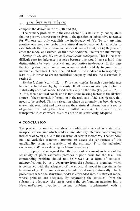
d�~y{Xbð Þ> W W>MX Wð Þ{1

W>� �

y{Xbð Þs2

u;

compare the denominator of (80) and (81).

The primary problem with the case where M1 is statistically inadequate is

that no positive answer can be given to the question of substantive relevance

for Wt; one can only establish the inadequacy of M0. To say anything

positive one needs to probe the statistical inadequacy of M1 in order to

establish whether the substantive factors Wt are relevant, but (i) they do not

enter the model as assumed, or (ii) other additional factors are still missing.

Setting 4: M1 and M0 are both statistically inadequate. This is the most

difficult case for inference purposes because one would have a hard time

distinguishing between statistical and substantive inadequacy. In this case

the testing discussion concerning scenarios A–E is likely to give rise to

unreliable inferences. Hence, the first task of the modeler is to respecify at

least M1, in order to ensure statistical adequacy and use the discussion in

setting 2.

Setting 5: Data {wt, t51, 2, …, T} are unavailable. In such a case inference

has to be based on M0 by necessity. If all tenacious attempts to find a

statistically adequate model based exclusively on the data {(xt, yt) t51, 2, …,

T} fail, then a natural conclusion is that some missing factors is the likeliest

source of the systematic information in the residuals of M0; a conjecture that

needs to be probed. This is a situation where an anomaly has been detected

(systematic residuals) and one can use the statistical information as a sourceof guidance in finding the relevant omitted factor(s). The situation is less

transparent in cases where M0 turns out to be statistically adequate.

6 CONCLUSION

The problem of omitted variables is traditionally viewed as a statisticalmisspecification issue which renders unreliable any inference concerning the

influence of Xt on yt due to the exclusion of certain factors Wt. The textbook

omitted variables argument attempts to assess the seriousness of this

unreliability using the sensitivity of the estimator bb to the inclusion/

exclusion of Wt as evidencing its bias/inconsistency.

In this paper, it is argued that the textbook argument in terms of thesensitivity of point estimates provides a poor basis for the task. The

confounding problem should not be viewed as a form of statistical

misspecification, but as a departure from the substantive premises, which

is concerned with the adequacy of the structural model in explaining the

behavior of yt. This issue can only be addressed using statistically reliable

procedures when the structural model is embedded into a statistical model

whose premises are adequate. By separating the statistical from the

substantive adequacy, the paper recasts the confounding question into aNeyman-Pearson hypothesis testing problem, supplemented with a

216 Articles

post-data evaluation of inference based on severe testing. Using an empirical

example it is shown how this testing perspective can deal effectively with

assessing the confounding issue. In the case where one of the two models,estimated with and without the variables Wt, is statistically misspecified, the

choice of inference methods becomes important. This provides a way to

motivate the use of different test procedures, such as the likelihood ratio,

Wald and Lagrange Multiplier methods, under different misspecification

scenarios.

Aris Spanos

Virginia Tech

aris@vt.edu

ACKNOWLEDGEMENTS

I would like to thank Kevin D. Hoover for numerous valuable comments/

suggestions on a previous draft which helped to improve the paper

considerably.

NOTES

1 The actual evaluations are based on: tc Zð Þ > bcc.dSE bccð ÞSE bccð Þ

� �{ c1

.dSE bccð ÞSE bccð Þ

� �h i;

�

c~c1Þ; the evaluation is at c5c1, because for values c>c1 the severity

increases.

2 The actual evaluations are based on:

tb Zð Þƒ bbb

dSE bbb� �

SE bbb� ��

{ b1

d

SE bbb� �

SE bbb� �� � �

; b~b1

�

REFERENCES

Cox, D.R. and Hinkley, D.V. (1974) Theoretical Statistics, London: Chapman &Hall.

Doob, J.L. (1953) Stochastic Processes, New York: Wiley.Fisher, R.A. (1935) The Design of Experiments, Edinburgh: Oliver and Boyd.Greene, W.H. (1997) Econometric Analysis. 3rd edn, NJ: Prentice Hall.Hoover, K.D. (2001) Causality in Macroeconomics, Cambridge: Cambridge

University Press.Johnston, J. (1984) Econometric Methods. 3rd edn, New York: McGraw-Hill.Leamer, E.E. (1978) Specification Searches: Ad Hoc Inference with Nonexperimental

Data, New York: Wiley.Leamer, E.E. and Leonard, H.B. (1983) ‘Reporting the fragility of regression

estimates’, Review of Economics and Statistics 65: 306–17.

Revisiting omitted variables 217

Mayo, D.G. (1991) ‘Novel evidence and severe tests,’, Philosophy of Science 58:523–52.

Mayo, D.G. (1996) Error and the Growth of Experimental Knowledge, Chicago: TheUniversity of Chicago Press.

Mayo, D.G. and Spanos, A. (2004) ‘Methodology in practice: statisticalmisspecification testing’, Philosophy of Science 71: 1007–25.

Mayo, D.G. and Spanos, A. (2006) ‘Severe testing as a basic concept in the Neyman-Pearson philosophy of induction,’, The British Journal for the Philosophy ofScience. (forthcoming).

Pagan, A. (1984) ‘Model Evaluation by Variable Addition,’, in Hendry, D.F. andWallis, K.F. (eds) Econometrics and Quantitative Economics, Oxford: BasilBlackwell, pp. 103–35.

Pearl, J. (2000) Causality: Models, Reasoning and Inference, Cambridge: CambridgeUniversity Press.

Spanos, A. (1986) Statistical Foundations of Econometric Modelling, Cambridge:Cambridge University Press.

Spanos, A. (1989) ‘On re-reading Haavelmo: a retrospective view of econometricmodeling’, Econometric Theory 5: 405–29.

Spanos, A. (1990) ‘The simultaneous equations model revisited: statistical adequacyand identification’, Journal of Econometrics 44: 87–108.

Spanos, A. (1995a) ‘On theory testing in econometrics: modeling with nonexperi-mental data’, Journal of Econometrics 67: 189–226.

Spanos, A. (1995b) ‘On normality and the Linear Regression model’, EconometricReviews 14: 195–203.

Spanos, A. (1999) Probability Theory and Statistical Inference: Econometric Modelingwith Observational Data, Cambridge: Cambridge University Press.

Spanos, A. (2005a) ‘Misspecification and the reliability of inference: the t-test in thepresence of Markov dependence,’, Virginia Tech Working Paper.

Spanos, A. (2005b) ‘Omitted variables and artificial regressions: a general approachto misspecification testing,’ Virginia Tech Working Paper.

Spanos, A. (2005c) ‘Structural equation modeling, causal inference and statisticaladequacy,’ P. Hajek, L. Valdes-Villanueva and D. Westerstahl (eds) Logic,Methodology and Philosophy of Science: Proceedings of the Twelfth InternationalCongress, London: King’s College, pp. 639–61.

Spanos, A. (2005d) ‘Structural vs. statistical models in empirical modeling: Kepler’sfirst law of planetery motion revisited,’ Virginia Tech working paper.

Spanos, A. (2006a) ‘Econometrics in retrospect and prospect,’ in Palgrave Handbookof Econometrics, vol. 1: Theoretical Econometrics, London: MacMillan, pp. 3–58.

Spanos, A. (2006b) ‘The instrumental variables method revisited: on the nature andchoice of optimal instruments’, in G.D.A. Phillips (ed.) Essays in Memory ofMichael Magdalinos, Cambridge: Cambridge University Press. (forthcoming).

Spanos, A. (2006c) ‘Where do statistical models come from? Revisiting the problemof specification’, in, The Second Erich L. Lehmann Symposium. vol. ##, Instituteof Mathematical Statistics. (forthcoming).

Spanos, A. and McGuirk, A. (2002) ‘The problem of near-multicollinearity revisited:erratic vs systematic volatility’, The Journal of Econometrics 108: 365–93.

Spirtes, P., Glymor, C. and Scheines, R. (2000) Causation, Prediction and Search. 2ndedn, Cambridge, MA: The MIT Press.

Stock, J.H. and Watson, M.W. (2002) Introduction to Econometrics, Boston, MA:Addison Wesley.

Wooldridge, J.M. (2003) Introductory Econometrics: A Modern Approach. 2nd edn,South-Western, OH: Thomson.

218 Articles