Embed Size (px)
Citation preview
Revisiting the Common Neighbour Analysis and the
Centrosymmetry Parameter
Peter M Larsen
Department of Physics, Technical University of Denmark, 2800 Kgs. Lyngby,
Denmark
E-mail: [email protected]
Abstract. We review two standard methods for structural classification in
simulations of crystalline phases, the Common Neighbour Analysis and the
Centrosymmetry Parameter. We explore the definitions and implementations of each of
their common variants, and investigate their respective failure modes and classification
biases. Simple modifications to both methods are proposed, which improve their
robustness, interpretability, and applicability. We denote these variants the Interval
Common Neighbour Analysis, and the Minimum-Weight Matching Centrosymmetry
Parameter.
arX
iv:2
003.
0887
9v1
[ph
ysic
s.co
mp-
ph]
19
Mar
202
0
Revisiting the Common Neighbour Analysis and the Centrosymmetry Parameter 2
1. Introduction
Extraction of useful material properties in a molecular dynamics (MD) simulation of
condensed phases requires that we can classify crystal structures. The lowest level of
this analysis is to resolve the structure at the atomic level, which is a prerequisite for
determining meso- and macro-scale properties such yield strength [1, 2] and hardness [3],
evolution in dislocation structures [4, 5] and grain structures [6, 7], and irradiation
damage [8].
Two structural analysis methods are particularly notable for their ubiquity:
Common Neighbour Analysis (CNA) [9] and the Centrosymmetry Parameter (CSP) [10].
These are amongst the first structural analysis methods to exploit crystal geometry, and
remain the most widely used despite the development of more advanced methods based
on topology [11, 12], geometry [13, 14, 15], statistical geometric (or machine-learning)
descriptors [16, 17, 18, 19, 20], and persistent homology [21, 22]. To a large extent,
these methods have endured due to their speed, simplicity, and being either parameter-
free (CNA) or single-parameter (CSP) methods. Even when not used directly, they
commonly serve as benchmarks for the development of new structural analysis methods.
In this paper we revisit the CNA and CSP methods. We describe their functionality
and perform a comprehensive analysis of their respective failure modes, and propose
some simple modifications which fix most of them. In doing so, we extend the
applicability and usefulness of both methods, and raise the baseline against which new
methods can be compared.
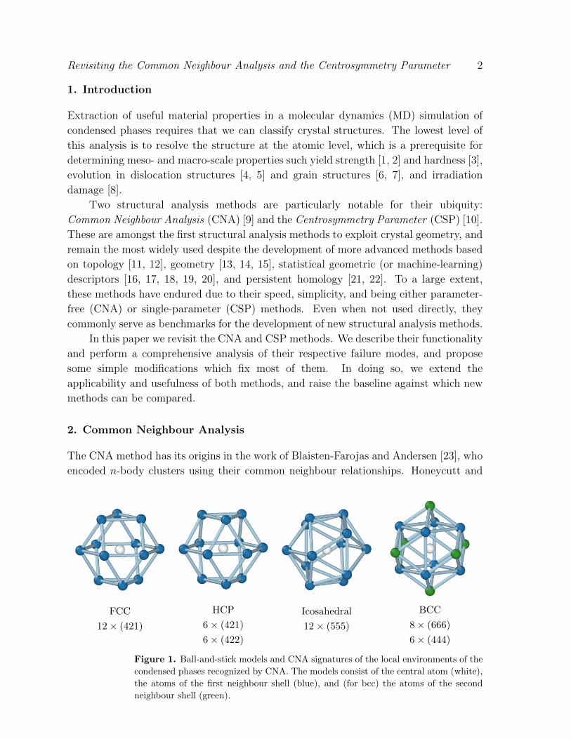
2. Common Neighbour Analysis
The CNA method has its origins in the work of Blaisten-Farojas and Andersen [23], who
encoded n-body clusters using their common neighbour relationships. Honeycutt and
FCC
12× (421)
HCP
6× (421)
6× (422)
Icosahedral
12× (555)
BCC
8× (666)
6× (444)
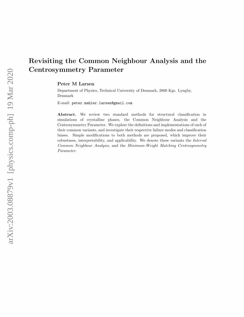
Figure 1. Ball-and-stick models and CNA signatures of the local environments of the
condensed phases recognized by CNA. The models consist of the central atom (white),
the atoms of the first neighbour shell (blue), and (for bcc) the atoms of the second
neighbour shell (green).
Revisiting the Common Neighbour Analysis and the Centrosymmetry Parameter 3
Andersen [24] generalized this approach to a larger set of clusters and used their relative
abundances to characterize structural order in nanoparticles. The currently used form of
CNA is due to Faken and Jonsson [9], who further extended the method to characterize
the local environment of a central atom.
The CNA method employs a ball-and-stick model: each neighbour atom (ball) is
joined to its nearest neighbours by a bond (stick). To identify the structure of an
atom in a simulation, its ball-and-stick model is constructed and compared against the
reference structures. This comparison is best described as a graph isomorphism test,
but for historical reasons the comparison is made by computing a signature of common
neighbour relationships. The signature consists of three indices per neighbour atom:
the number of bonded neighbours shared with the central atom, the number of bonds
between shared neighbours, and the number of bonds in the longest chain formed by
shared neighbours. The ball-and-stick models and their associated CNA signatures are
shown in Figure 1.
In a perfect crystal, the radial distribution function (RDF) contains well-separated
peaks, which makes it easy to identify the appropriate bonded pairs. In a MD simulation,
however, the atoms must necessarily move from their ideal positions. To account for the
resulting variability in the distance between bonded pairs, a threshold rc is introduced
which defines nearest neighbours as those whose distance satisfies r < rc. Honeycutt
and Andersen set rc to the first minimum in the (RDF), which lies between the first
and second neighbour shells. The use of a single, global threshold is commonly referred
to as the Conventional Common Neighbour Analysis (c-CNA) method.
For some simulations it is not possible to define a single consistent threshold. For
example, in multi-phase systems with differing lattice constants, the peaks in the RDF
are not well-separated. To account for this variation in scale, Stukowski introduced the
Adaptive Common Neighbour Analysis (a-CNA) [25], which computes a local threshold
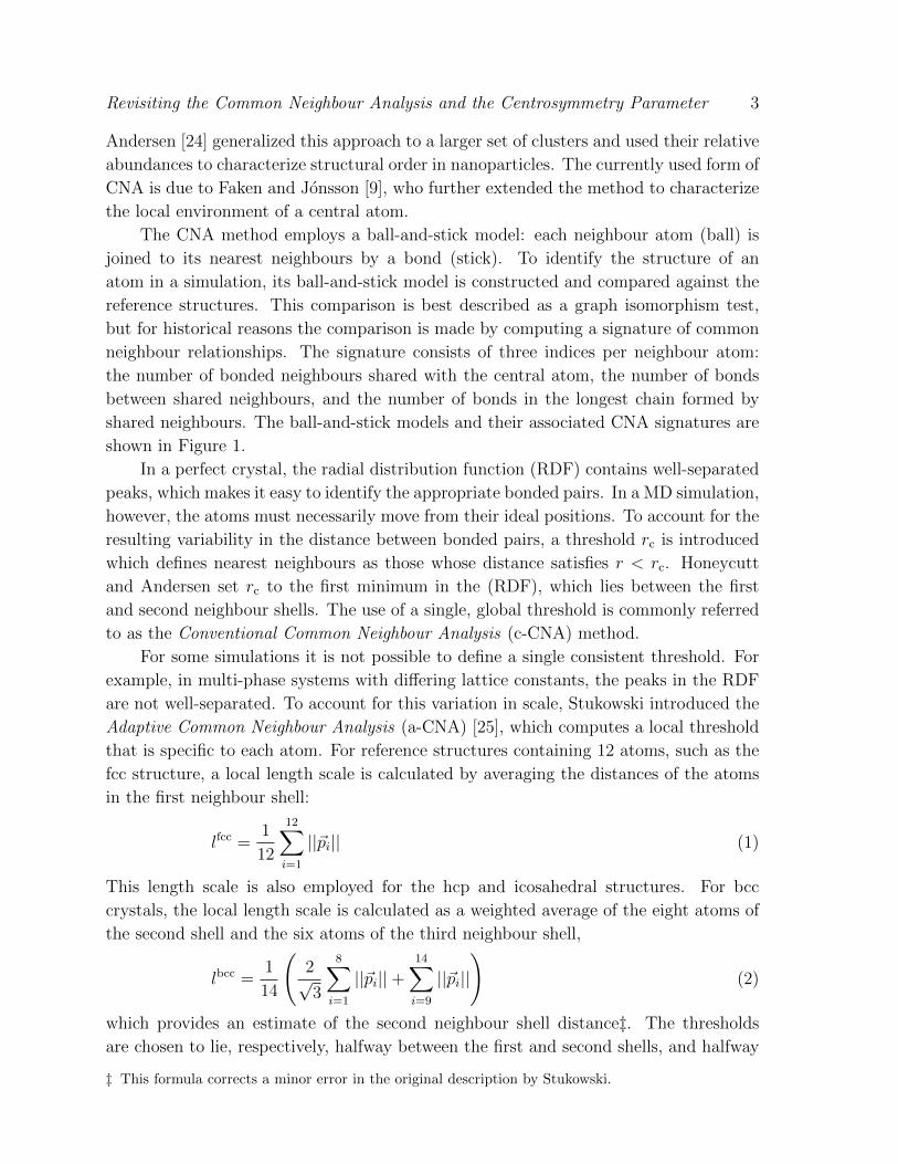
that is specific to each atom. For reference structures containing 12 atoms, such as the
fcc structure, a local length scale is calculated by averaging the distances of the atoms
in the first neighbour shell:
lfcc =1
12
12∑i=1
||~pi|| (1)
This length scale is also employed for the hcp and icosahedral structures. For bcc
crystals, the local length scale is calculated as a weighted average of the eight atoms of
the second shell and the six atoms of the third neighbour shell,
lbcc =1
14
(2√3
8∑i=1
||~pi||+14∑i=9
||~pi||
)(2)
which provides an estimate of the second neighbour shell distance‡. The thresholds
are chosen to lie, respectively, halfway between the first and second shells, and halfway
‡ This formula corrects a minor error in the original description by Stukowski.
Revisiting the Common Neighbour Analysis and the Centrosymmetry Parameter 4
r/lfcc
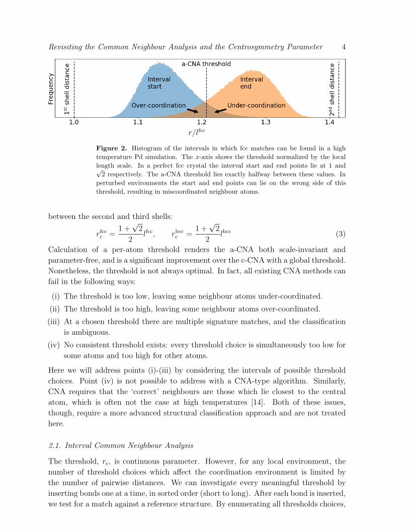
Figure 2. Histogram of the intervals in which fcc matches can be found in a high
temperature Pd simulation. The x-axis shows the threshold normalized by the local
length scale. In a perfect fcc crystal the interval start and end points lie at 1 and√2 respectively. The a-CNA threshold lies exactly halfway between these values. In
perturbed environments the start and end points can lie on the wrong side of this
threshold, resulting in miscoordinated neighbour atoms.
between the second and third shells:
rfccc =1 +√
2
2lfcc, rbccc =
1 +√
2
2lbcc (3)
Calculation of a per-atom threshold renders the a-CNA both scale-invariant and
parameter-free, and is a significant improvement over the c-CNA with a global threshold.
Nonetheless, the threshold is not always optimal. In fact, all existing CNA methods can
fail in the following ways:
(i) The threshold is too low, leaving some neighbour atoms under-coordinated.
(ii) The threshold is too high, leaving some neighbour atoms over-coordinated.
(iii) At a chosen threshold there are multiple signature matches, and the classification
is ambiguous.
(iv) No consistent threshold exists: every threshold choice is simultaneously too low for
some atoms and too high for other atoms.
Here we will address points (i)-(iii) by considering the intervals of possible threshold
choices. Point (iv) is not possible to address with a CNA-type algorithm. Similarly,
CNA requires that the ‘correct’ neighbours are those which lie closest to the central
atom, which is often not the case at high temperatures [14]. Both of these issues,
though, require a more advanced structural classification approach and are not treated
here.
2.1. Interval Common Neighbour Analysis
The threshold, rc, is continuous parameter. However, for any local environment, the
number of threshold choices which affect the coordination environment is limited by
the number of pairwise distances. We can investigate every meaningful threshold by
inserting bonds one at a time, in sorted order (short to long). After each bond is inserted,
we test for a match against a reference structure. By enumerating all thresholds choices,
Revisiting the Common Neighbour Analysis and the Centrosymmetry Parameter 5
σ
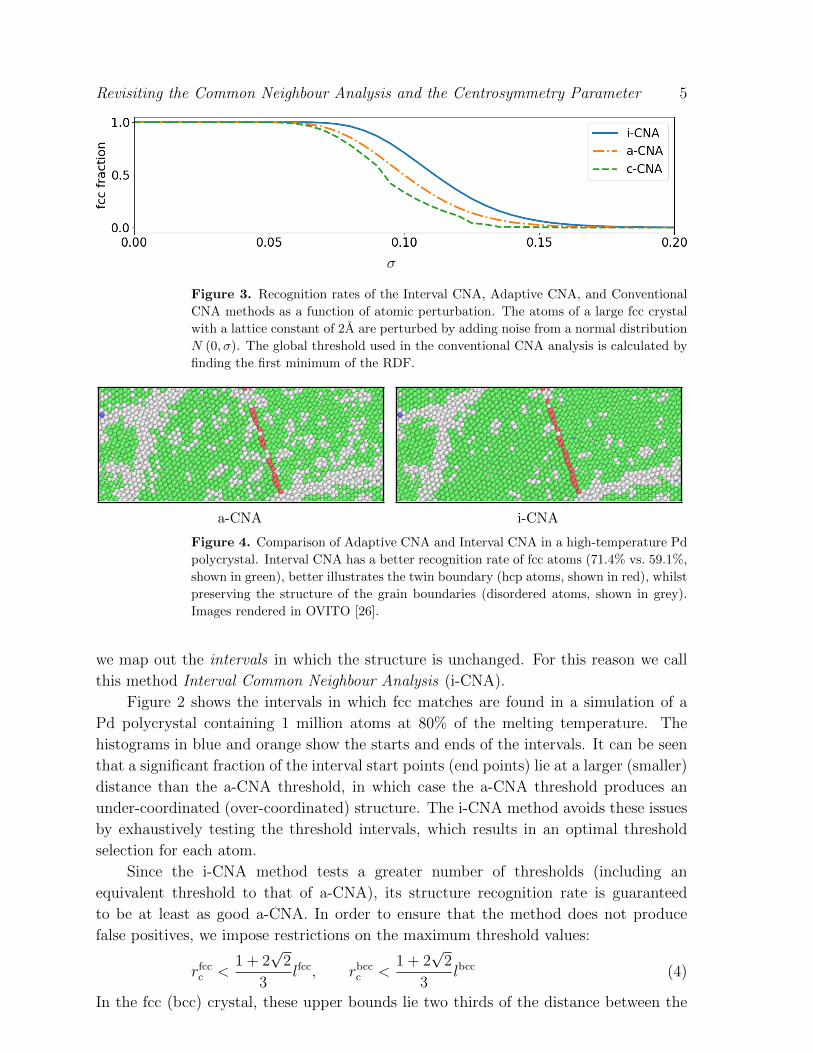
Figure 3. Recognition rates of the Interval CNA, Adaptive CNA, and Conventional
CNA methods as a function of atomic perturbation. The atoms of a large fcc crystal
with a lattice constant of 2A are perturbed by adding noise from a normal distribution
N (0, σ). The global threshold used in the conventional CNA analysis is calculated by
finding the first minimum of the RDF.
a-CNA i-CNA
Figure 4. Comparison of Adaptive CNA and Interval CNA in a high-temperature Pd
polycrystal. Interval CNA has a better recognition rate of fcc atoms (71.4% vs. 59.1%,
shown in green), better illustrates the twin boundary (hcp atoms, shown in red), whilst
preserving the structure of the grain boundaries (disordered atoms, shown in grey).
Images rendered in OVITO [26].
we map out the intervals in which the structure is unchanged. For this reason we call
this method Interval Common Neighbour Analysis (i-CNA).
Figure 2 shows the intervals in which fcc matches are found in a simulation of a
Pd polycrystal containing 1 million atoms at 80% of the melting temperature. The
histograms in blue and orange show the starts and ends of the intervals. It can be seen
that a significant fraction of the interval start points (end points) lie at a larger (smaller)
distance than the a-CNA threshold, in which case the a-CNA threshold produces an
under-coordinated (over-coordinated) structure. The i-CNA method avoids these issues
by exhaustively testing the threshold intervals, which results in an optimal threshold
selection for each atom.
Since the i-CNA method tests a greater number of thresholds (including an
equivalent threshold to that of a-CNA), its structure recognition rate is guaranteed
to be at least as good a-CNA. In order to ensure that the method does not produce
false positives, we impose restrictions on the maximum threshold values:
rfccc <1 + 2
√2
3lfcc, rbccc <
1 + 2√
2
3lbcc (4)
In the fcc (bcc) crystal, these upper bounds lie two thirds of the distance between the
Revisiting the Common Neighbour Analysis and the Centrosymmetry Parameter 6
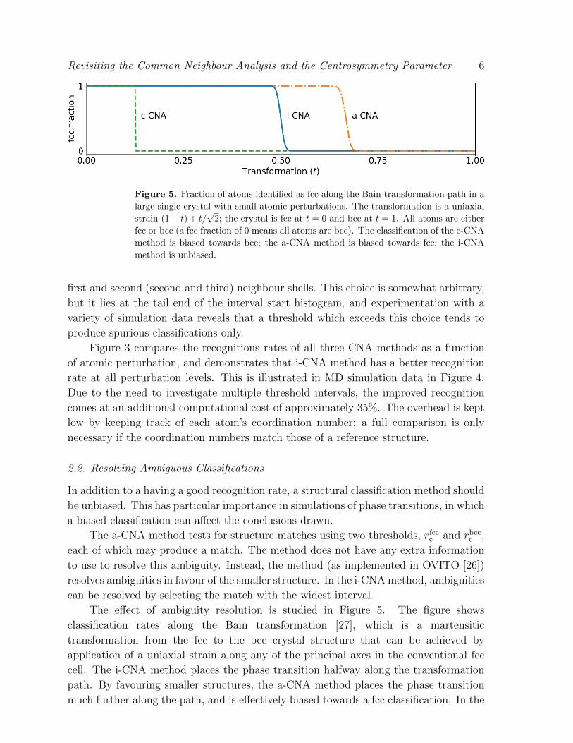
Figure 5. Fraction of atoms identified as fcc along the Bain transformation path in a
large single crystal with small atomic perturbations. The transformation is a uniaxial
strain (1− t) + t/√
2; the crystal is fcc at t = 0 and bcc at t = 1. All atoms are either
fcc or bcc (a fcc fraction of 0 means all atoms are bcc). The classification of the c-CNA
method is biased towards bcc; the a-CNA method is biased towards fcc; the i-CNA
method is unbiased.
first and second (second and third) neighbour shells. This choice is somewhat arbitrary,
but it lies at the tail end of the interval start histogram, and experimentation with a
variety of simulation data reveals that a threshold which exceeds this choice tends to
produce spurious classifications only.
Figure 3 compares the recognitions rates of all three CNA methods as a function
of atomic perturbation, and demonstrates that i-CNA method has a better recognition
rate at all perturbation levels. This is illustrated in MD simulation data in Figure 4.
Due to the need to investigate multiple threshold intervals, the improved recognition
comes at an additional computational cost of approximately 35%. The overhead is kept
low by keeping track of each atom’s coordination number; a full comparison is only
necessary if the coordination numbers match those of a reference structure.
2.2. Resolving Ambiguous Classifications
In addition to a having a good recognition rate, a structural classification method should
be unbiased. This has particular importance in simulations of phase transitions, in which
a biased classification can affect the conclusions drawn.
The a-CNA method tests for structure matches using two thresholds, rfccc and rbccc ,
each of which may produce a match. The method does not have any extra information
to use to resolve this ambiguity. Instead, the method (as implemented in OVITO [26])
resolves ambiguities in favour of the smaller structure. In the i-CNA method, ambiguities
can be resolved by selecting the match with the widest interval.
The effect of ambiguity resolution is studied in Figure 5. The figure shows
classification rates along the Bain transformation [27], which is a martensitic
transformation from the fcc to the bcc crystal structure that can be achieved by
application of a uniaxial strain along any of the principal axes in the conventional fcc
cell. The i-CNA method places the phase transition halfway along the transformation
path. By favouring smaller structures, the a-CNA method places the phase transition
much further along the path, and is effectively biased towards a fcc classification. In the
Revisiting the Common Neighbour Analysis and the Centrosymmetry Parameter 7
c-CNA method, a fcc classification is not possible as soon as 14 neighbours lie within the
threshold distance. Here, there is no ambiguity to resolve but the method is strongly
biased towards a bcc classification.
3. The Centrosymmetry Parameter
The CSP is a structural analysis method which takes an opposite approach to CNA.
Rather than using a set of reference structures to classify the topology of the local
atomic environment, it computes an order parameter which quantifies the degree of
inversion (or centro) symmetry of the local environment. In the original formulation of
Kelchner et al., the CSP is defined using the N = 12 nearest neighbours of a central
atom:
CSP (R) =6∑
i=1
||~ri + ~ri+6||2 (5)
where ~ri and ~ri+6 are the vectors ‘corresponding to the six pairs of opposite nearest
neighbours in the fcc lattice’ [10]. For the bcc lattice the summation is replaced by
the eight nearest neighbours. For other centrosymmetric structures the appropriate
summation is similarly intuitive, as each nearest neighbour atom has a clearly defined
opposite neighbour.
There are two commonly used algorithms for calculating the CSP. The first
algorithm (described in ref. [25]) calculates a weight wij = ||~ri + ~rj|| for each of the
N(N − 1)/2 pairs of neighbour atoms, and calculates the CSP as the summation over
the N/2 smallest weights. Reproduction of the Au defects described in ref. [10] reveals
that this approach was used by Kelchner et al. The second algorithm (described in
ref. [28]) proceeds by ordering the atoms by their distance from the central atom;
opposite pairs are found by (i) pairing the inner-most atom with its minimal-weight
partner, (ii) removing this pair, and (iii) repeating the process until no atoms are left.
The first method is implemented in LAMMPS [29] and OVITO [26]. We will
describe this method as the Greedy Edge Selection (GES) CSP. The second method is
implemented in AtomEye [30] and Atomsk [31]. We will describe this method as the
Greedy Vertex Matching (GVM) CSP. The GVM implementation typically employs a
normalization constant1
2∑i
||~ri||2(6)
which renders the CSP invariant to scale, but, in highly centrosymmetric structures at
least, these methods are otherwise equivalent.
3.1. The Graph Matching Centrosymmetry Parameter
The definition in Equation (5) describes the CSP for centrosymmetric structures, but
does not specify how the CSP should be calculated in the general case. The CSP is
Revisiting the Common Neighbour Analysis and the Centrosymmetry Parameter 8
Minimum-weight matching
CSP=0.39
Greedy edge selection
CSP=0.32
Greedy vertex matching
CSP=4.36
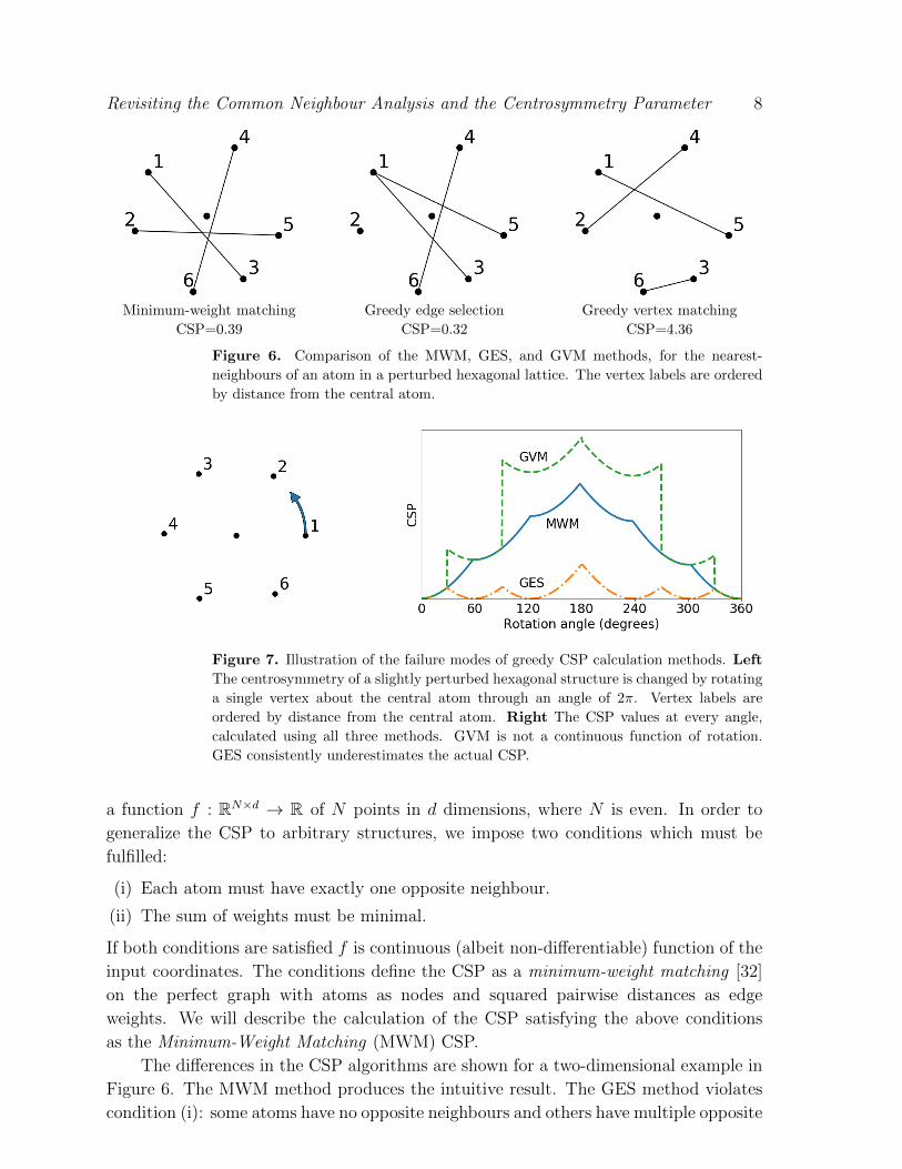
Figure 6. Comparison of the MWM, GES, and GVM methods, for the nearest-
neighbours of an atom in a perturbed hexagonal lattice. The vertex labels are ordered
by distance from the central atom.
Figure 7. Illustration of the failure modes of greedy CSP calculation methods. Left
The centrosymmetry of a slightly perturbed hexagonal structure is changed by rotating
a single vertex about the central atom through an angle of 2π. Vertex labels are
ordered by distance from the central atom. Right The CSP values at every angle,
calculated using all three methods. GVM is not a continuous function of rotation.
GES consistently underestimates the actual CSP.
a function f : RN×d → R of N points in d dimensions, where N is even. In order to
generalize the CSP to arbitrary structures, we impose two conditions which must be
fulfilled:
(i) Each atom must have exactly one opposite neighbour.
(ii) The sum of weights must be minimal.
If both conditions are satisfied f is continuous (albeit non-differentiable) function of the
input coordinates. The conditions define the CSP as a minimum-weight matching [32]
on the perfect graph with atoms as nodes and squared pairwise distances as edge
weights. We will describe the calculation of the CSP satisfying the above conditions
as the Minimum-Weight Matching (MWM) CSP.
The differences in the CSP algorithms are shown for a two-dimensional example in
Figure 6. The MWM method produces the intuitive result. The GES method violates
condition (i): some atoms have no opposite neighbours and others have multiple opposite
Revisiting the Common Neighbour Analysis and the Centrosymmetry Parameter 9
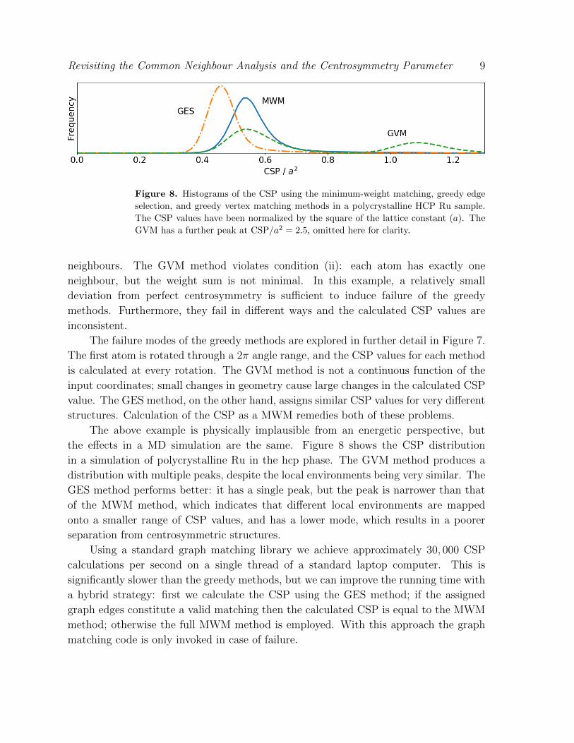
Figure 8. Histograms of the CSP using the minimum-weight matching, greedy edge
selection, and greedy vertex matching methods in a polycrystalline HCP Ru sample.
The CSP values have been normalized by the square of the lattice constant (a). The
GVM has a further peak at CSP/a2 = 2.5, omitted here for clarity.
neighbours. The GVM method violates condition (ii): each atom has exactly one
neighbour, but the weight sum is not minimal. In this example, a relatively small
deviation from perfect centrosymmetry is sufficient to induce failure of the greedy
methods. Furthermore, they fail in different ways and the calculated CSP values are
inconsistent.
The failure modes of the greedy methods are explored in further detail in Figure 7.
The first atom is rotated through a 2π angle range, and the CSP values for each method
is calculated at every rotation. The GVM method is not a continuous function of the
input coordinates; small changes in geometry cause large changes in the calculated CSP
value. The GES method, on the other hand, assigns similar CSP values for very different
structures. Calculation of the CSP as a MWM remedies both of these problems.
The above example is physically implausible from an energetic perspective, but
the effects in a MD simulation are the same. Figure 8 shows the CSP distribution
in a simulation of polycrystalline Ru in the hcp phase. The GVM method produces a
distribution with multiple peaks, despite the local environments being very similar. The
GES method performs better: it has a single peak, but the peak is narrower than that
of the MWM method, which indicates that different local environments are mapped
onto a smaller range of CSP values, and has a lower mode, which results in a poorer
separation from centrosymmetric structures.
Using a standard graph matching library we achieve approximately 30, 000 CSP
calculations per second on a single thread of a standard laptop computer. This is
significantly slower than the greedy methods, but we can improve the running time with
a hybrid strategy: first we calculate the CSP using the GES method; if the assigned
graph edges constitute a valid matching then the calculated CSP is equal to the MWM
method; otherwise the full MWM method is employed. With this approach the graph
matching code is only invoked in case of failure.
Revisiting the Common Neighbour Analysis and the Centrosymmetry Parameter 10
4. Conclusions
We have analyzed the behaviour of the CNA and CSP methods, and presented
some simple extensions which improve their usefulness without introducing any extra
parameters. By performing an exhaustive threshold search, the i-CNA method
achieves a better structural recognition rate in local environments with larger atomic
perturbations. Furthermore, we introduced the Bain transformation as a test for
classification bias, and it was shown that i-CNA is unbiased.
For the CSP, we demonstrated that the existing calculation methods do not produce
consistent results. Using methods from graph theory, we proposed a solution which is
continuous with respect to atomic perturbations and produces an intuitive result at any
level of centrosymmetry.
Acknowledgments
The author thanks for Alexander Stukowski for helpful discussions and Daniel Utt for
providing Pd simulation data. This work was supported by Grant No. 7026-00126B
from the Danish Council for Independent Research.
References
[1] Schiøtz J, Di Tolla F D and Jacobsen K W 1998 Nature 391 561–563
[2] Li X, Wei Y, Lu L, Lu K and Gao H 2010 Nature 464 877–880
[3] Kallman J S, Hoover W G, Hoover C G, De Groot A J, Lee S M and Wooten F 1993 Phys. Rev.
B 47(13) 7705–7709
[4] Stukowski A, Bulatov V V and Arsenlis A 2012 Model. Simul. Mater. Sci. Eng 20 085007
[5] Zepeda-Ruiz L A, Stukowski A, Oppelstrup T and Bulatov V V 2017 Nature 550 492–495
[6] Panzarino J F, Ramos J J and Rupert T J 2015 Model. Simul. Mater. Sci. Eng 23 025005
[7] Chesser I, Holm E A and Demkowicz M J 2020 Acta Mat. 183 207 – 215
[8] Marian J, Wirth B D, Schublin R, Odette G and Perlado J 2003 J. Nucl. Mater 323 181–191
[9] Faken D and Jonsson H 1994 Comput. Mater. Sci. 2 279 – 286
[10] Kelchner C L, Plimpton S J and Hamilton J C 1998 Phys. Rev. B 58(17) 11085–11088
[11] Malins A, Williams S R, Eggers J and Royall C P 2013 J. Chem. Phys. 139 234506
[12] Lazar E A 2017 Model. Simul. Mater. Sci. Eng 26 015011
[13] Ackland G J and Jones A P 2006 Phys. Rev. B 73(5) 054104
[14] Larsen P M, Schmidt S and Schiøtz J 2016 Model. Simul. Mater. Sci. Eng 24 055007
[15] Martelli F, Ko H Y, Oguz E C and Car R 2018 Phys. Rev. B 97(6) 064105
[16] Steinhardt P J, Nelson D R and Ronchetti M 1983 Phys. Rev. B 28(2) 784–805
[17] Bartok A P, Kondor R and Csanyi G 2013 Phys. Rev. B 87(18) 184115
[18] Spellings M and Glotzer S C 2018 AIChE J. 64 2198–2206
[19] Ceriotti M 2019 J. Chem. Phys. 150 150901
[20] Adorf C S, Moore T C, Melle Y J U and Glotzer S C 2020 J. Phys. Chem. B 124 69–78
[21] Buchet M, Hiraoka Y and Obayashi I 2018 Persistent Homology and Materials Informatics
(Singapore: Springer Singapore) pp 75–95 ISBN 978-981-10-7617-6
[22] Maroulas V, Micucci C P and Spannaus A 2019 Adv. Data Anal. Classi.
[23] Blaisten-Barojas E and Andersen H C 1985 Surf. Sci. 156 548 – 555
[24] Honeycutt J D and Andersen H C 1987 J. Phys. Chem. 91 4950–4963
Revisiting the Common Neighbour Analysis and the Centrosymmetry Parameter 11
[25] Stukowski A 2012 Model. Simul. Mater. Sci. Eng 20 045021
[26] Stukowski A 2009 Model. Simul. Mater. Sci. Eng 18 015012
[27] Bain E C and Dunkirk N 1924 Trans. AIME 70 25–47
[28] Bulatov V and Cai W 2006 Computer Simulations of Dislocations (Oxford University Press) ISBN
978-0198526148
[29] Plimpton S 1995 J. Comput. Phys. 117 1–19
[30] Li J 2003 Model. Simul. Mater. Sci. Eng 11 173–177
[31] Hirel P 2015 Comput. Phys. Commun. 197 212–219
[32] Edmonds J 1965 J. Res. Nat. Bur. Standards B 69 125–130