1

REVISION CHAPTER

ALGEBRA

LEARNING OUTCOMES

Upon completing this topic, the students will be able to:

1. Differentiate between the types of mathematic function (PLO1-K-C3)

2. Manipulate algebraic expressions by using all of algebra rules (PLO1-K-

C3)

3. Separate an algebraic fraction into its partial fractions (PLO1-K-C3)

1.0 INTRODUCTION

Chapter 1 is started with section 1.1 which is about introduction to the types

of function in mathematics. Then, followed by the review of algebra rules in

section 1.2. Finally, in section 1.3, partial fraction will be discussed. A set

of tutorial for chapter 1 is available in section 1.4

1.1 TYPES OF FUNCTION

The purpose of this reference section is to show you graphs of various

types of functions in order that you can become familiar with the types.

You will discover that each type has its own distinctive graph. By showing

several graphs on one plot you will be able to see their common features.

Examples of the following types of functions are shown in this chapter:

linear

quadratic

power

polynomial

rational

exponential

logarithmic

sinusoidal

2

In each case the argument (input) of the function is called x and the value

(output) of the function is called y.

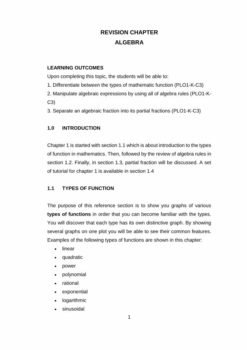
1.1.1 LINEAR FUNCTION

These are functions of the form:

y = m x + b,

where m and b are constants. A typical use for linear functions is converting

from one quantity or set of units to another. Graphs of these functions are

straight lines (see Figure 1.1). m is the slope and b is the y intercept. If m

is positive then the line rises to the right and if m is negative then the line

falls to the right.

Figure 1.1 Linear graph

3

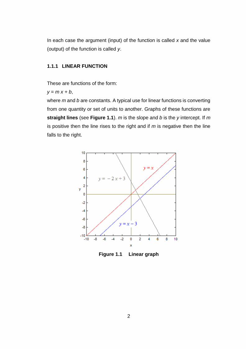
1.1.2 QUADRATIC FUNCTION

These are functions of the form:

y = a x 2 + b x + c,

where a, b and c are constants. Their graphs are called parabolas (see

Figure 1.2). This is the next simplest type of function after the linear

function. Falling objects move along parabolic paths. If a is a positive

number then the parabola opens upward and if a is a negative number

then the parabola opens downward.

Figure 1.2 Quadratic graph

1.1.3 POWER FUNCTION

These are functions of the form:

y = a x b,

where a and b are constants. They get their name from the fact that the

variable x is raised to some power. Many physical laws (e.g. the

gravitational force as a function of distance between two objects, or the

bending of a beam as a function of the load on it) are in the form of power

functions. We will assume that a = 1 and look at several cases for b:

4

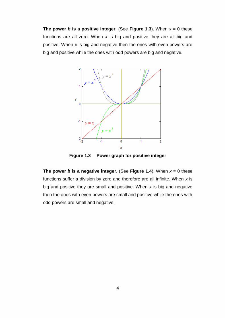
The power b is a positive integer. (See Figure 1.3). When x = 0 these

functions are all zero. When x is big and positive they are all big and

positive. When x is big and negative then the ones with even powers are

big and positive while the ones with odd powers are big and negative.

Figure 1.3 Power graph for positive integer

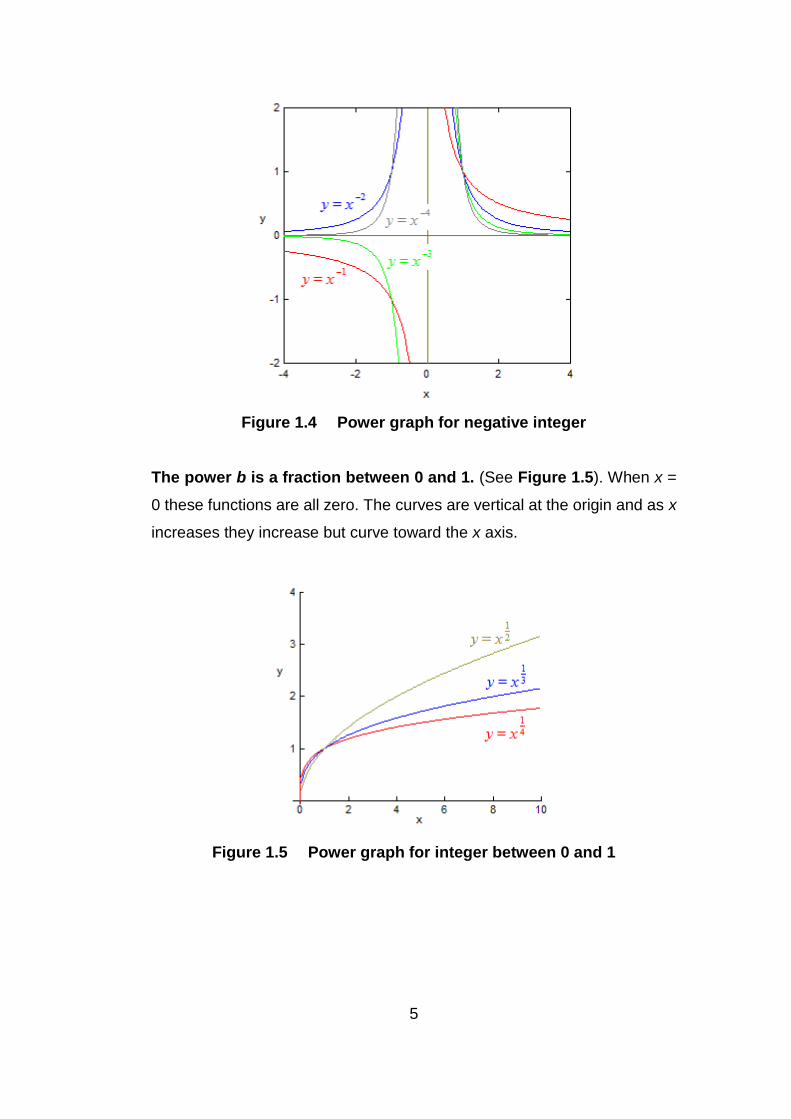
The power b is a negative integer. (See Figure 1.4). When x = 0 these

functions suffer a division by zero and therefore are all infinite. When x is

big and positive they are small and positive. When x is big and negative

then the ones with even powers are small and positive while the ones with

odd powers are small and negative.

5

Figure 1.4 Power graph for negative integer

The power b is a fraction between 0 and 1. (See Figure 1.5). When x =

0 these functions are all zero. The curves are vertical at the origin and as x

increases they increase but curve toward the x axis.

Figure 1.5 Power graph for integer between 0 and 1

6

1.1.4 POLYNOMIAL FUNCTION

These are functions of the form:

y = an · x n + an −1 · x n −1 + … + a2 · x 2 + a1 · x + a0,

where an, an −1, … , a2, a1, a0 are constants. Only whole number powers of

x are allowed. The highest power of x that occurs is called the degree of

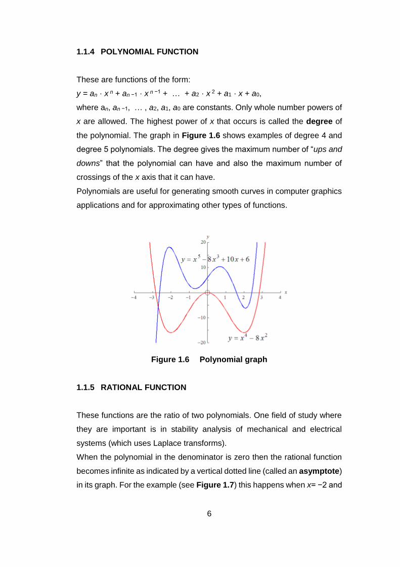
the polynomial. The graph in Figure 1.6 shows examples of degree 4 and

degree 5 polynomials. The degree gives the maximum number of “ups and

downs” that the polynomial can have and also the maximum number of

crossings of the x axis that it can have.

Polynomials are useful for generating smooth curves in computer graphics

applications and for approximating other types of functions.

Figure 1.6 Polynomial graph

1.1.5 RATIONAL FUNCTION

These functions are the ratio of two polynomials. One field of study where

they are important is in stability analysis of mechanical and electrical

systems (which uses Laplace transforms).

When the polynomial in the denominator is zero then the rational function

becomes infinite as indicated by a vertical dotted line (called an asymptote)

in its graph. For the example (see Figure 1.7) this happens when x= −2 and

7

when x = 7. When x becomes very large the curve may level off. The curve

to the right levels off at y = 5.

Figure 1.7 Rational graph with horizontal asymptote at y=5 and

vertical asymptote at x= −2 and x = 7

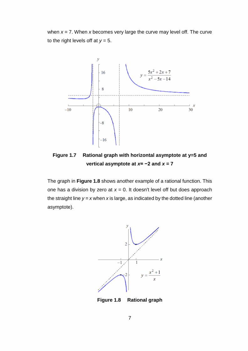
The graph in Figure 1.8 shows another example of a rational function. This

one has a division by zero at x = 0. It doesn't level off but does approach

the straight line y = x when x is large, as indicated by the dotted line (another

asymptote).

Figure 1.8 Rational graph

8

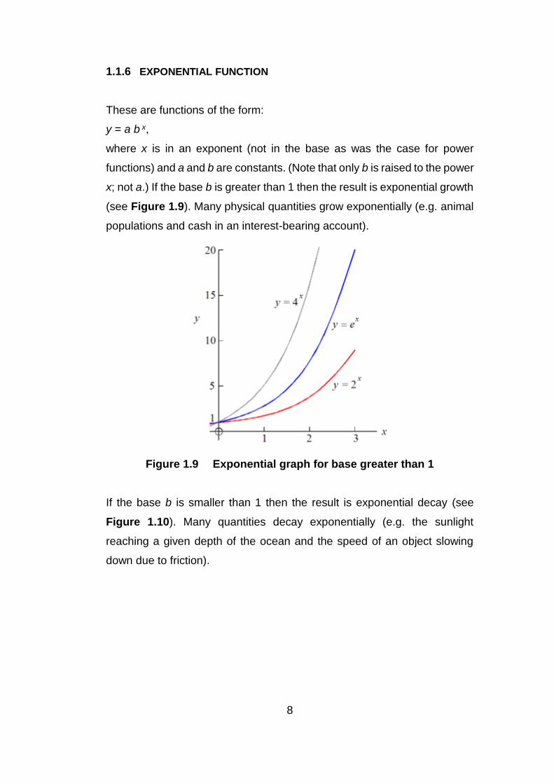
1.1.6 EXPONENTIAL FUNCTION

These are functions of the form:

y = a b x,

where x is in an exponent (not in the base as was the case for power

functions) and a and b are constants. (Note that only b is raised to the power

x; not a.) If the base b is greater than 1 then the result is exponential growth

(see Figure 1.9). Many physical quantities grow exponentially (e.g. animal

populations and cash in an interest-bearing account).

Figure 1.9 Exponential graph for base greater than 1

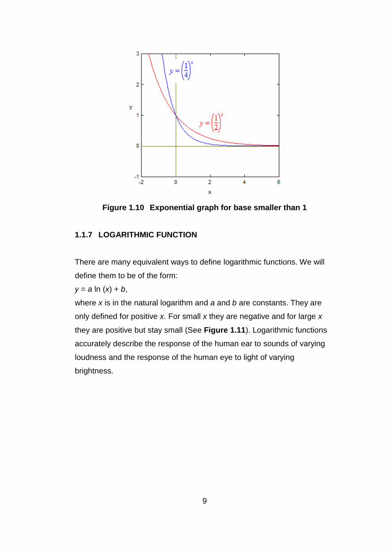
If the base b is smaller than 1 then the result is exponential decay (see

Figure 1.10). Many quantities decay exponentially (e.g. the sunlight

reaching a given depth of the ocean and the speed of an object slowing

down due to friction).

9

Figure 1.10 Exponential graph for base smaller than 1

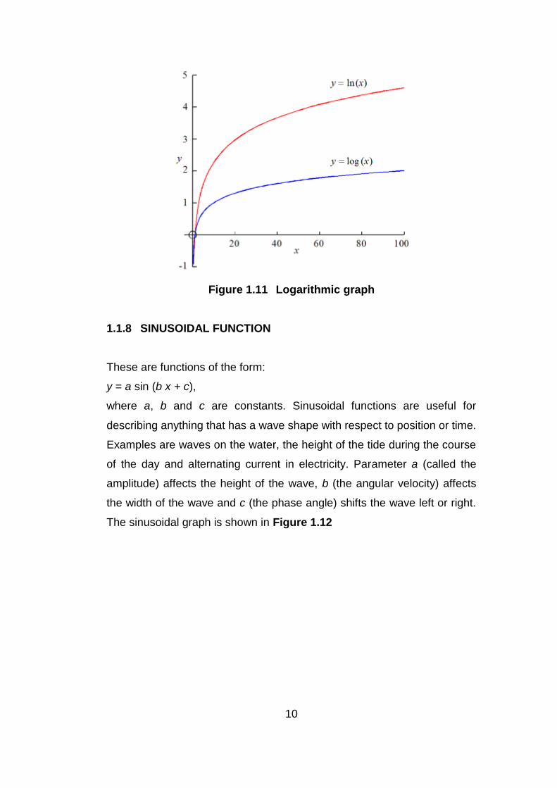
1.1.7 LOGARITHMIC FUNCTION

There are many equivalent ways to define logarithmic functions. We will

define them to be of the form:

y = a ln (x) + b,

where x is in the natural logarithm and a and b are constants. They are

only defined for positive x. For small x they are negative and for large x

they are positive but stay small (See Figure 1.11). Logarithmic functions

accurately describe the response of the human ear to sounds of varying

loudness and the response of the human eye to light of varying

brightness.

10

Figure 1.11 Logarithmic graph

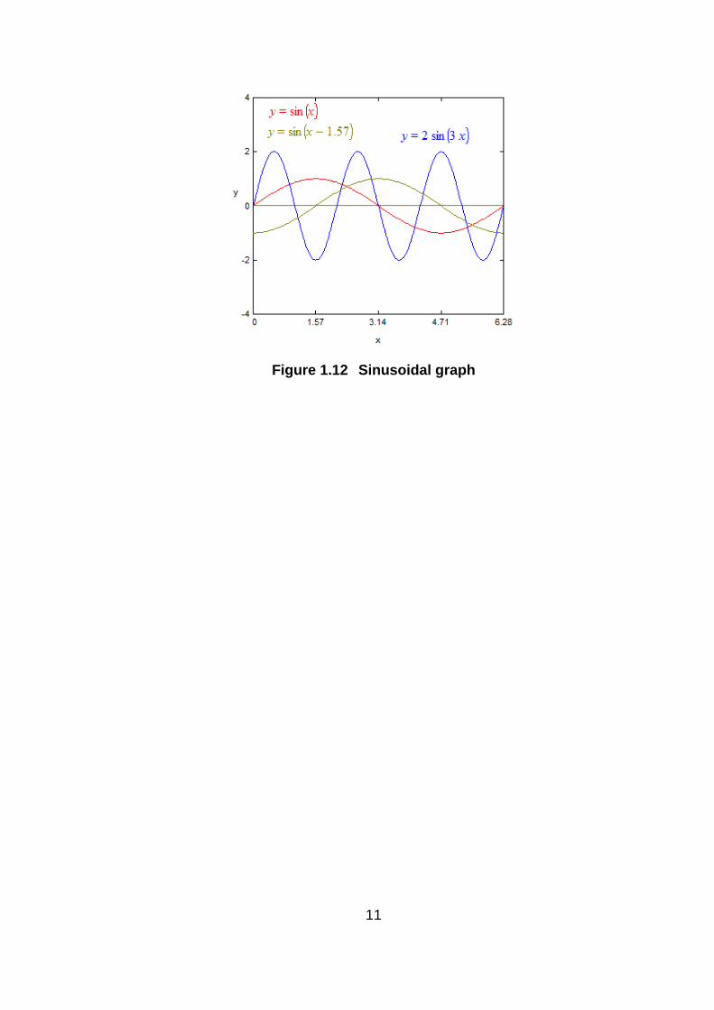
1.1.8 SINUSOIDAL FUNCTION

These are functions of the form:

y = a sin (b x + c),

where a, b and c are constants. Sinusoidal functions are useful for

describing anything that has a wave shape with respect to position or time.

Examples are waves on the water, the height of the tide during the course

of the day and alternating current in electricity. Parameter a (called the

amplitude) affects the height of the wave, b (the angular velocity) affects

the width of the wave and c (the phase angle) shifts the wave left or right.

The sinusoidal graph is shown in Figure 1.12

11

Figure 1.12 Sinusoidal graph

12

1.2 REVIEW OF ALGEBRA

Here we review the basic rules and procedures of algebra that you need

to know in order to be successful in calculus.

1.2.1 ARITHMETIC OPERATIONS

The real numbers have the following properties:

𝑎 + 𝑏 = 𝑏 + 𝑎 𝑎𝑏 = 𝑏𝑎 (Commutative Law)

(𝑎 + 𝑏) + 𝑐 = 𝑎 + (𝑏 + 𝑐) (𝑎𝑏)𝑐 = 𝑎(𝑏𝑐) (Associative Law)

𝑎(𝑏 + 𝑐) = 𝑎𝑏 + 𝑎𝑐 (Distributive law)

In particular, putting 𝑎 = −1 in the Distributive Law, we get

−(𝑏 + 𝑐) = (−1)(𝑏 + 𝑐) = (−1)𝑏 + (−1)𝑐

and so

−(𝑏 + 𝑐) = −𝑏 − 𝑐

Example 1.1

i. (3𝑥𝑦)(−4𝑥) = 3(−4)𝑥2𝑦 = −12𝑥2𝑦

ii. 2𝑡(7𝑥 + 2𝑡𝑥 − 11) = 14𝑡𝑥 + 4𝑡2 − 22𝑡

iii. 4 − 3(𝑥 − 2) = 4 − 3𝑥 + 6 = 10 − 3𝑥

If we use the Distributive Law three times, we get

(𝑎 + 𝑏)(𝑐 + 𝑑) = (𝑎 + 𝑏)𝑐 + (𝑎 + 𝑏)𝑑 = 𝑎𝑐 + 𝑏𝑐 + 𝑎𝑑 + 𝑏𝑑

This says that we multiply two factors by multiplying each term in one

factor by each term in the other factor and adding the products.

In the case where 𝑐 = 𝑎 and 𝑑 = 𝑏, we have

(𝑎 + 𝑏)2 = 𝑎2 + 𝑏𝑎 + 𝑎𝑏 + 𝑏2 = 𝑎2 + 2𝑎𝑏 + 𝑏2

Similarly, we obtain

(𝑎 − 𝑏)2 = 𝑎2 − 2𝑎𝑏 + 𝑏2

13

Exercise 1.1

Solve these using appropriate law.

i. (2𝑥 + 1)(3𝑥 − 5)

ii. (𝑥 + 6)2

iii. 3(𝑥 − 1)(4𝑥 + 3) − 2(𝑥 + 6)

1.2.2 FRACTIONS

To add two fractions with the same denominator, we use the Distributive

Law:

𝑎

𝑏+

𝑐

𝑏=

1

𝑏× 𝑎 +

1

𝑏× 𝑐 =

1

𝑏(𝑎 + 𝑐) =

𝑎 + 𝑐

𝑏

Thus, it is true that

𝑎 + 𝑐

𝑏=

𝑎

𝑏+

𝑐

𝑏

But remember to avoid the following common error:

𝑎

𝑏 + 𝑐≠

𝑎

𝑏+

𝑐

𝑏

(For instance, take 𝑎 = 𝑏 = 𝑐 = 1 to see the error.)

To add two fractions with different denominators, we use a common

denominator:

𝑎

𝑏+

𝑐

𝑑=

𝑎𝑑 + 𝑏𝑐

𝑏𝑑

We multiply such fractions as follows:

𝑎

𝑏∗

𝑐

𝑑=

𝑎𝑐

𝑏𝑑

In particular, it is true that

−𝑎

𝑏= −

𝑎

𝑏=

𝑎

−𝑏

To divide two fractions, we invert and multiply:

𝑎𝑏𝑐𝑑

=𝑎

𝑏×

𝑑

𝑐=

𝑎𝑑

𝑏𝑐

14

Example 1.2

i. 𝑥+3

𝑥=

𝑥

𝑥+

3

𝑥= 1 +

3

𝑥

ii. 𝑠2𝑡

𝑢∗

𝑢𝑡

−2=

𝑠2𝑡2𝑢

−2𝑢= −

𝑠2𝑡2

2

Exercise 2.2

i. 3

𝑥−1+

𝑥

𝑥+2

ii.

𝑥

𝑦+1

1−𝑦

𝑥

1.2.3 FACTORING

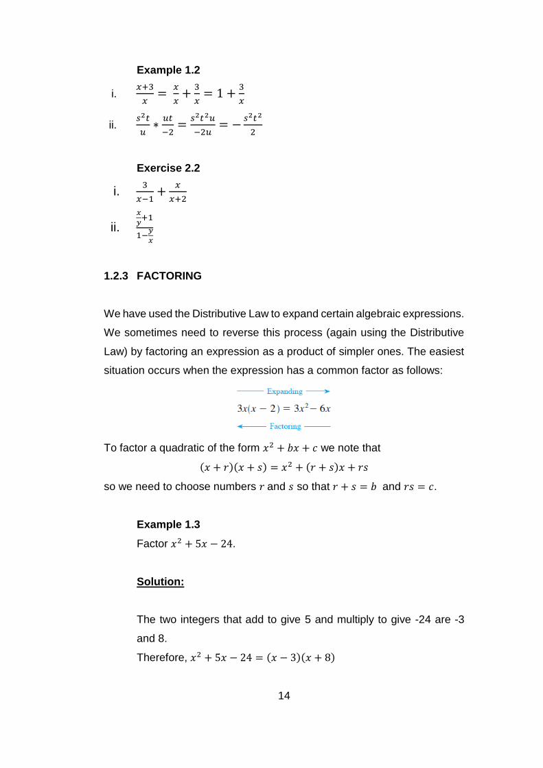
We have used the Distributive Law to expand certain algebraic expressions.

We sometimes need to reverse this process (again using the Distributive

Law) by factoring an expression as a product of simpler ones. The easiest

situation occurs when the expression has a common factor as follows:

To factor a quadratic of the form 𝑥2 + 𝑏𝑥 + 𝑐 we note that

(𝑥 + 𝑟)(𝑥 + 𝑠) = 𝑥2 + (𝑟 + 𝑠)𝑥 + 𝑟𝑠

so we need to choose numbers 𝑟 and 𝑠 so that 𝑟 + 𝑠 = 𝑏 and 𝑟𝑠 = 𝑐.

Example 1.3

Factor 𝑥2 + 5𝑥 − 24.

Solution:

The two integers that add to give 5 and multiply to give -24 are -3

and 8.

Therefore, 𝑥2 + 5𝑥 − 24 = (𝑥 − 3)(𝑥 + 8)

15

Example 1.4

Factor 2𝑥2 − 7𝑥 − 4.

Solution:

Even though the coefficient of is not 1, we can still look for factors of

the form 2𝑥 + 𝑟 and 𝑥 + 𝑠, where 𝑟𝑠 = −4. Experimentation reveals

that

2𝑥2 − 7𝑥 − 4 = (2𝑥 + 1)(𝑥 − 4)

Some special quadratics can be factored by using the formula for a

difference of squares:

a. a2 − b2 = (a − b)(a + b)

b. a3 − b3 = (a − b)(a2 + ab + b2)

c. a3 + b3 = (a + b)(a2 − ab + b2)

Exercise 1.3

i. 𝑥2 − 6𝑥 + 9

ii. 4𝑥2 − 25

iii. 𝑥3 + 8

Example 1.5

Simplify 𝑥2−16

𝑥2−2𝑥−8

Solution:

Factoring numerator and denominator, we have

𝑥2 − 16

𝑥2 − 2𝑥 − 8=

(𝑥 − 4)(𝑥 + 4)

(𝑥 − 4)(𝑥 + 2)=

𝑥 + 4

𝑥 + 2

To factor polynomials of degree 3 or more, we sometimes use the

following fact:

THE FACTOR THEOREM: If 𝑃 is a polynomial and 𝑃(𝑏) = 0, then

𝑥 − 𝑏 is a factor of 𝑃(𝑥)

16

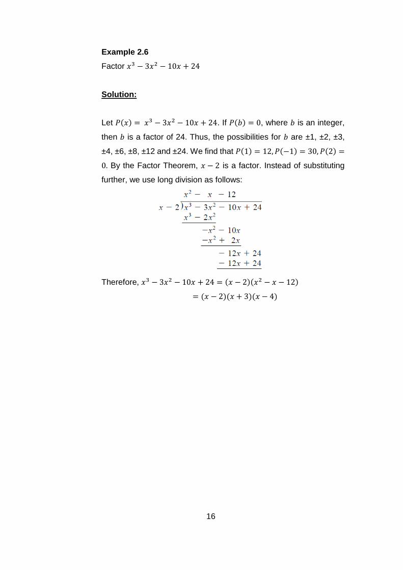
Example 2.6

Factor 𝑥3 − 3𝑥2 − 10𝑥 + 24

Solution:

Let 𝑃(𝑥) = 𝑥3 − 3𝑥2 − 10𝑥 + 24. If 𝑃(𝑏) = 0, where 𝑏 is an integer,

then 𝑏 is a factor of 24. Thus, the possibilities for 𝑏 are ±1, ±2, ±3,

±4, ±6, ±8, ±12 and ±24. We find that 𝑃(1) = 12, 𝑃(−1) = 30, 𝑃(2) =

0. By the Factor Theorem, 𝑥 − 2 is a factor. Instead of substituting

further, we use long division as follows:

Therefore, 𝑥3 − 3𝑥2 − 10𝑥 + 24 = (𝑥 − 2)(𝑥2 − 𝑥 − 12)

= (𝑥 − 2)(𝑥 + 3)(𝑥 − 4)

17

1.2.4 COMPLETING THE SQUARE

Completing the square is a useful technique for graphing parabolas or

integrating rational functions. Completing the square means rewriting a

quadratic 𝑎𝑥2 + 𝑏𝑥 + 𝑐 in the form 𝑎(𝑥 + 𝑝)2 + 𝑞 and can be accomplished

by:

1. Factoring the number from the terms involving 𝑥.

2. Adding and subtracting the square of half the coefficient of 𝑥.

In general, we have

𝑎𝑥2 + 𝑏𝑥 + 𝑐 = 𝑎 [𝑥2 +𝑏

𝑎𝑥] + 𝑐

= 𝑎 [𝑥2 +𝑏

𝑎𝑥 + (

𝑏

2𝑎)2 − (

𝑏

2𝑎)2] + 𝑐

= 𝑎(𝑥 +𝑏

2𝑎)2 + (𝑐 −

𝑏2

4𝑎)

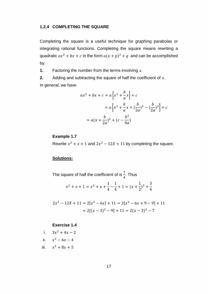
Example 1.7

Rewrite 𝑥2 + 𝑥 + 1 and 2𝑥2 − 12𝑋 + 11 by completing the square.

Solutions:

The square of half the coefficient of is 1

4. Thus

𝑥2 + 𝑥 + 1 = 𝑥2 + 𝑥 +1

4−

1

4+ 1 = (𝑥 +

1

2)2 +

3

4

2𝑥2 − 12𝑋 + 11 = 2[𝑥2 − 6𝑥] + 11 = 2[𝑥2 − 6𝑥 + 9 − 9] + 11

= 2[(𝑥 − 3)2 − 9] + 11 = 2(𝑥 − 3)2 − 7

Exercise 1.4

i. 3𝑥2 + 4𝑥 − 2

ii. 𝑥2 − 6𝑥 − 4

iii. 𝑥2 + 8𝑥 + 5

18

1.2.5 RADICALS

The most commonly occurring radicals are square roots. The symbol √

means “the positive square root of.” Thus

𝑥 = √𝑎 𝑚𝑒𝑎𝑛𝑠 𝑥2 = 𝑎 𝑎𝑛𝑑 𝑥 ≥ 0

Since 𝑎 = 𝑥2 ≥ 0, the symbol √𝑎 makes sense only when 𝑎 ≥ 0 . Here are

two rules for working with square roots:

a. √𝑎𝑏 = √𝑎√𝑏

b. √𝑎

𝑏=

√𝑎

√𝑏

However, there is no similar rule for the square root of a sum. In fact, you

should remember to avoid the following common error:

√𝑎 + 𝑏 ≠ √𝑎 + √𝑏

(For instance, take 𝑎 = 9 and 𝑏 = 16 to see the error.)

Example 1.8

i. √18

√2= √

18

2= √9 = 3

ii. √𝑥2𝑦 = √𝑥2 √𝑦 = 𝑥√𝑦

In general, if 𝑛 is a positive integer,

𝑥 = √𝑎 𝑛

𝑚𝑒𝑎𝑛𝑠 𝑥𝑛 = 𝑎

√𝑎𝑏𝑛

= √𝑎𝑛 √𝑏

𝑛 & √

𝑎

𝑏

𝑛=

√𝑎𝑛

√𝑏𝑛

To rationalize a numerator or denominator that contains an expression

such as √𝑎 − √𝑏 , we multiply both the numerator and the denominator by

the conjugate radical √𝑎 + √𝑏. Then we can take advantage of the formula

for a difference of squares:

(√𝑎 − √𝑏)(√𝑎 + √𝑏) = (√𝑎)2 − (√𝑏)2 = 𝑎 − 𝑏

19

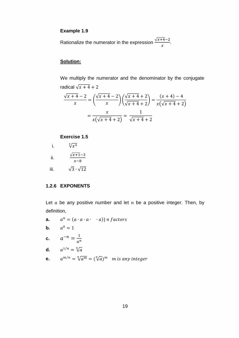
Example 1.9

Rationalize the numerator in the expression √𝑥+4−2

𝑥.

Solution:

We multiply the numerator and the denominator by the conjugate

radical √𝑥 + 4 + 2

√𝑥 + 4 − 2

𝑥= (

√𝑥 + 4 − 2

𝑥) (

√𝑥 + 4 + 2

√𝑥 + 4 + 2) =

(𝑥 + 4) − 4

𝑥(√𝑥 + 4 + 2)

=𝑥

𝑥(√𝑥 + 4 + 2)=

1

√𝑥 + 4 + 2

Exercise 1.5

i. √𝑥43

ii. √𝑥+1−3

𝑥−8

iii. √3 ∙ √12

1.2.6 EXPONENTS

Let 𝑎 be any positive number and let 𝑛 be a positive integer. Then, by

definition,

a. 𝑎𝑛 = (𝑎 ∙ 𝑎 ∙ 𝑎 ∙ ∙ 𝑎)} 𝑛 𝑓𝑎𝑐𝑡𝑜𝑟𝑠

b. 𝑎0 = 1

c. 𝑎−𝑛 =1

𝑎𝑛

d. 𝑎1 𝑛⁄ = √𝑎𝑛

e. 𝑎𝑚 𝑛⁄ = √𝑎𝑚𝑛= ( √𝑎

𝑛)𝑚 𝑚 𝑖𝑠 𝑎𝑛𝑦 𝑖𝑛𝑡𝑒𝑔𝑒𝑟

20

Laws of Exponents: Let 𝑎 and 𝑏 be positive numbers and let 𝑟 and 𝑠 be

any rational numbers (that is, ratios of integers). Then,

a. 𝑎𝑟 × 𝑎𝑠 = 𝑎𝑟+𝑠

b. 𝑎𝑟

𝑎𝑠= 𝑎𝑟−𝑠

c. (𝑎𝑟)𝑠 = 𝑎𝑟𝑠

d. (𝑎𝑏)𝑟 = 𝑎𝑟𝑏𝑟

e. (𝑎

𝑏)𝑟 =

𝑎𝑟

𝑏𝑟 𝑏 ≠ 0

In words, these five laws can be stated as follows:

1. To multiply two powers of the same number, we add the exponents.

2. To divide two powers of the same number, we subtract the exponents.

3. To raise a power to a new power, we multiply the exponents.

4. To raise a product to a power, we raise each factor to the power.

5. To raise a quotient to a power, we raise both numerator and denominator

to the power

Example 1.10

(𝑥

𝑦)3(

𝑦2𝑥

𝑧)4 =

𝑥3

𝑦3∙

𝑦8𝑥4

𝑧4= 𝑥7𝑦5𝑧−4

Exercise 1.6

i. 28 × 82

ii. 𝑥−2−𝑦−2

𝑥−1+𝑦−1

iii. 1

√𝑥43

21

1.3 PARTIAL FRACTION

Given a rational function, if the degree of the polynomial in the numerator

is less than the degree of the polynomial in the denominator, then the

rational function can be expressed as the sum of rational functions whose

denominators are powers of linear polynomials and powers of irreducible

quadratic functions. This sum is called the partial fraction decomposition of

the rational function.

Given the rational function 𝑟(𝑥) =𝑝(𝑥)

𝑞(𝑥).

If the factorization of the polynomial 𝑞(𝑥) contains 𝑚 identical linear factors,

𝑎𝑥 + 𝑏 then the partial fraction decomposition of 𝑟(𝑥) contains a sum of the

form:

𝐴1

𝑎𝑥 + 𝑏+

𝐴2

(𝑎𝑥 + 𝑏)2+

𝐴3

(𝑎𝑥 + 𝑏)3+∙∙∙∙∙ +

𝐴𝑚

(𝑎𝑥 + 𝑏)𝑚

Where 𝐴1, 𝐴2, 𝐴3, … . . , 𝐴𝑚 are constants to be determined.

If the factorization of the polynomial 𝑞(𝑥) contains 𝑚 identical irreducible

quadratic factors 𝑎𝑥2 + 𝑏𝑥 + 𝑐, then the partial fraction decomposition of

𝑟(𝑥) contains a sum of the form

𝐴1𝑥 + 𝐵1

𝑎𝑥2 + 𝑏𝑥 + 𝑐+

𝐴2𝑥 + 𝐵2

(𝑎𝑥2 + 𝑏𝑥 + 𝑐)2+∙∙∙∙∙ +

𝐴𝑚𝑥 + 𝐵𝑚

(𝑎𝑥2 + 𝑏𝑥 + 𝑐)𝑚

where 𝐴1, 𝐴2, … . . , 𝐴𝑚 and 𝐵1, 𝐵2, … . . , 𝐵𝑚 are constants to be determined.

22

Example 1.11

Evaluate the following function

6

𝑥2 − 9𝑥

Solution:

= 6

𝑥(𝑥 − 9)=

𝐴

𝑥+

𝐵

𝑥 − 9

We need to solve for A and B.

Multiplying both sides of the equation by 𝑥(𝑥 − 9), we obtain the

equation 6 = 𝐴(𝑥 − 9) + 𝐵𝑥. From here, there are two methods for

solving for A and B.

Method 1

The first method is to solve a system of equations obtained from

equating the coefficients of the terms on each side of the equation.

6 = 𝐴(𝑥 − 9) + 𝐵𝑥 → 6 = 𝐴𝑥 − 9𝐴 + 𝐵𝑥 → 6 = (𝐴 + 𝐵)𝑥 − 9𝐴

The coefficient of the x term on the right side of the equation is 𝐴 +

𝐵. Since there is not an x term on the left side of the equation, then

its coefficient is zero. Equating the coefficients of the x terms on each

side of the equation, we obtain that. 𝐴 + 𝐵 = 0. The constant term

on the right side of the equation is −9𝐴. The constant term on the

left side of the equation is 6. Equating the constant terms on each

side of the equation, we obtain that −9𝐴 = 6. Thus, to solve for A

and B, we will solve the system of equations 𝐴 + 𝐵 = 0 and −9𝐴 =

6. The second equation gives us that = −2

3 . The first equation

gives us that 𝐵 = −𝐴 =2

3.

23

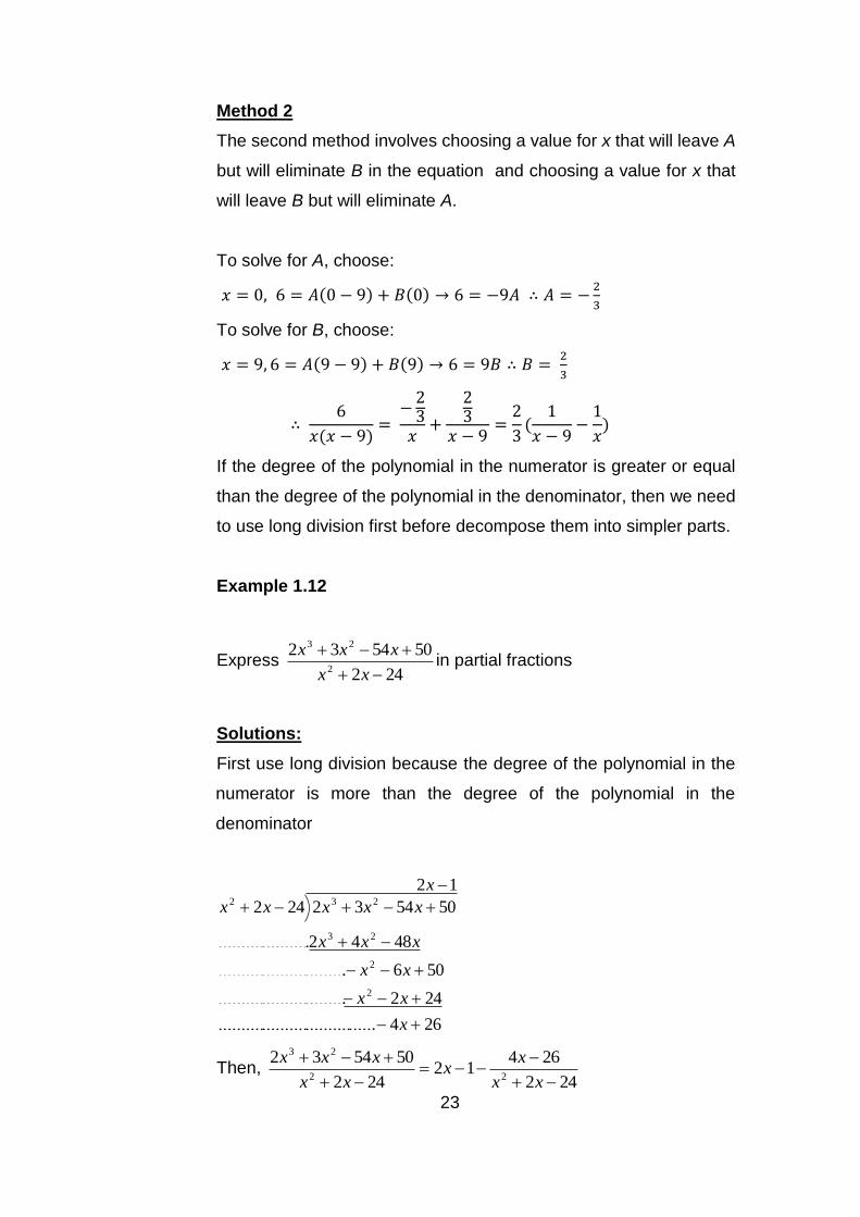
Method 2

The second method involves choosing a value for x that will leave A

but will eliminate B in the equation and choosing a value for x that

will leave B but will eliminate A.

To solve for A, choose:

𝑥 = 0, 6 = 𝐴(0 − 9) + 𝐵(0) → 6 = −9𝐴 ∴ 𝐴 = −2

3

To solve for B, choose:

𝑥 = 9, 6 = 𝐴(9 − 9) + 𝐵(9) → 6 = 9𝐵 ∴ 𝐵 = 2

3

∴ 6

𝑥(𝑥 − 9)=

−23

𝑥+

23

𝑥 − 9=

2

3(

1

𝑥 − 9−

1

𝑥)

If the degree of the polynomial in the numerator is greater or equal

than the degree of the polynomial in the denominator, then we need

to use long division first before decompose them into simpler parts.

Example 1.12

Express 242

5054322

23

xx

xxxin partial fractions

Solutions:

First use long division because the degree of the polynomial in the

numerator is more than the degree of the polynomial in the

denominator

264....................................

242.............................

506.............................

4842.....................

12

505432242

2

2

23

232

x

xx

xx

xxx

x

xxxxx

Then, 242

26412

242

50543222

23

xx

xx

xx

xxx

24

64)6)(4(

264

x

B

x

A

xx

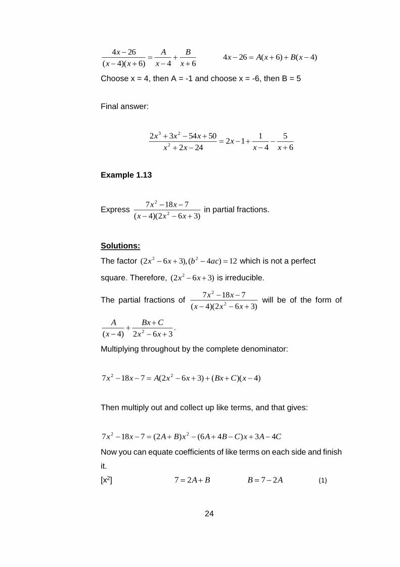
x )4()6(264 xBxAx

Choose x = 4, then A = -1 and choose x = -6, then B = 5

Final answer:

6

5

4

112

242

5054322

23

xxx

xx

xxx

Example 1.13

Express )362)(4(

71872

2

xxx

xx in partial fractions.

Solutions:

The factor 12)4(),362( 22 acbxx which is not a perfect

square. Therefore, )362( 2 xx is irreducible.

The partial fractions of )362)(4(

71872

2

xxx

xx will be of the form of

362)4( 2

xx

CBx

x

A.

Multiplying throughout by the complete denominator:

)4)(()362(7187 22 xCBxxxAxx

Then multiply out and collect up like terms, and that gives:

CAxCBAxBAxx 43)46()2(7187 22

Now you can equate coefficients of like terms on each side and finish

it.

[x2] BA 27 AB 27 (1)

25

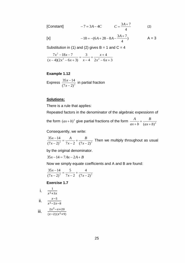
[Constant] CA 437 4

73

AC (2)

[x] )4

738286(18

AAA A = 3

Substitution in (1) and (2) gives B = 1 and C = 4

362

4

4

3

)362)(4(

718722

2

xx

x

xxxx

xx

Example 1.12

Express 2)27(

1435

x

x in partial fraction

Solutions:

There is a rule that applies:

Repeated factors in the denominator of the algebraic expessionn of

the form 2)( bax give partial fractions of the form 2)( bax

B

bax

A

Consequently, we write:

22 )27(27)27(

1435

x

B

x

A

x

x Then we multiply throughout as usual

by the original denominator.

BAAxx 271435

Now we simply equate coefficients and A and B are found:

22 )27(

4

27

5

)27(

1435

xxx

x

Exercise 1.7

i. 1

𝑥2+3𝑥

ii. 𝑥−5

𝑥2−2𝑥−8

iii. 2𝑥2−𝑥+20

(𝑥−2)(𝑥2+9)

26

1.4 TUTORIAL

a. Expand and simplify.

i. (−6𝑎𝑏)(0.5𝑎𝑐) ii. −(2𝑥2𝑦)(−𝑥𝑦4)

iii. 2𝑥(𝑥 − 5) iv. (4 − 3𝑥)𝑥

v. −2(4 − 3𝑎) vi. 8 − (4 + 𝑥)

vii. 4(𝑥2 − 𝑥 + 2) − 5(𝑥2 − 2𝑥 +

1)

viii. 5(3𝑡 − 4) − (𝑡2 + 2) −

2𝑡(𝑡 − 3)

ix. (4𝑥 − 1)(3𝑥 + 7) x. 𝑥(𝑥 − 1)(𝑥 + 2)

xi. (2𝑥 − 1)2 xii. (2 + 3𝑥)2

xiii. 𝑦4(6 − 𝑦)(5 + 𝑦) xiv. (𝑡 − 5)2 − 2(𝑡 + 3)(8𝑡 − 1)

xv. (𝑡 − 5)2 − 2(𝑡 + 3)(8𝑡 − 1) xvi. (1 + 2𝑥)(𝑥2 − 3𝑥 + 1)

b. Perform the indicated operations and simplify.

i. 2+8𝑥

2 ii.

9𝑏−6

3𝑏

iii. 1

𝑥+5+

2

𝑥−3 iv.

1

𝑥+1+

1

𝑥−1

v. 𝑢 + 1 +𝑢

𝑢+1 vi.

2

𝑎2−

3

𝑎𝑏+

4

𝑏2

vii. 𝑥 𝑦⁄

𝑧 viii.

𝑥

𝑦 𝑧⁄

ix. (−2𝑟

𝑠) (

𝑠2

−6𝑡) x.

𝑎

𝑏𝑐÷

𝑏

𝑎𝑐

xi. 1+

1

𝑐−1

1−1

𝑐−1

xii. 1 +

1

1+1

1+𝑥

27

c. Factor the expression.

i. 6𝑥2 − 5𝑥 − 6 ii. 𝑥2 + 10𝑥 + 25

iii. 𝑡3 + 1 iv. 4𝑡2 − 9𝑠2

v. 4𝑡2 − 12𝑡 + 9 vi. 𝑥3 − 27

vii. 𝑥3 + 2𝑥2 + 𝑥 viii. 𝑥3 − 4𝑥2 + 5𝑥 − 2

ix. 𝑥3 + 3𝑥2 − 𝑥 − 3 x. 𝑥3 − 2𝑥2 − 23𝑥 + 60

xi. 𝑥3 + 5𝑥2 − 2𝑥 − 24 xii. 𝑥3 − 3𝑥2 − 4𝑥 + 12

d. Simplify the expression.

i. 𝑥2+𝑥−2

𝑥2−3𝑥+2 ii.

2𝑥2−3𝑥−2

𝑥2−4

iii. 𝑥2−1

𝑥2−9𝑥+8 iv.

𝑥3+5𝑥2+6𝑥

𝑥2−𝑥−12

v. 1

𝑥+3+

1

𝑥2−9 vi.

𝑥

𝑥2+𝑥−2−

2

𝑥2−5𝑥+4

e. Complete the square.

i. 𝑥2 + 2𝑥 + 5 ii. 𝑥2 − 16𝑥 + 80

iii. 𝑥2 − 5𝑥 + 10 iv. 𝑥2 + 3𝑥 + 1

v. 4𝑥2 + 4𝑥 − 2 vi. 3𝑥2 − 24𝑥 + 50

f. Simplify the radicals.

i. √32√2 ii. √𝑥𝑦√𝑥3𝑦

iii. √−23

√543

iv. √16𝑎4𝑏3

v. √32𝑥44

√24 vi.

√96𝑎65

√3𝑎5

28

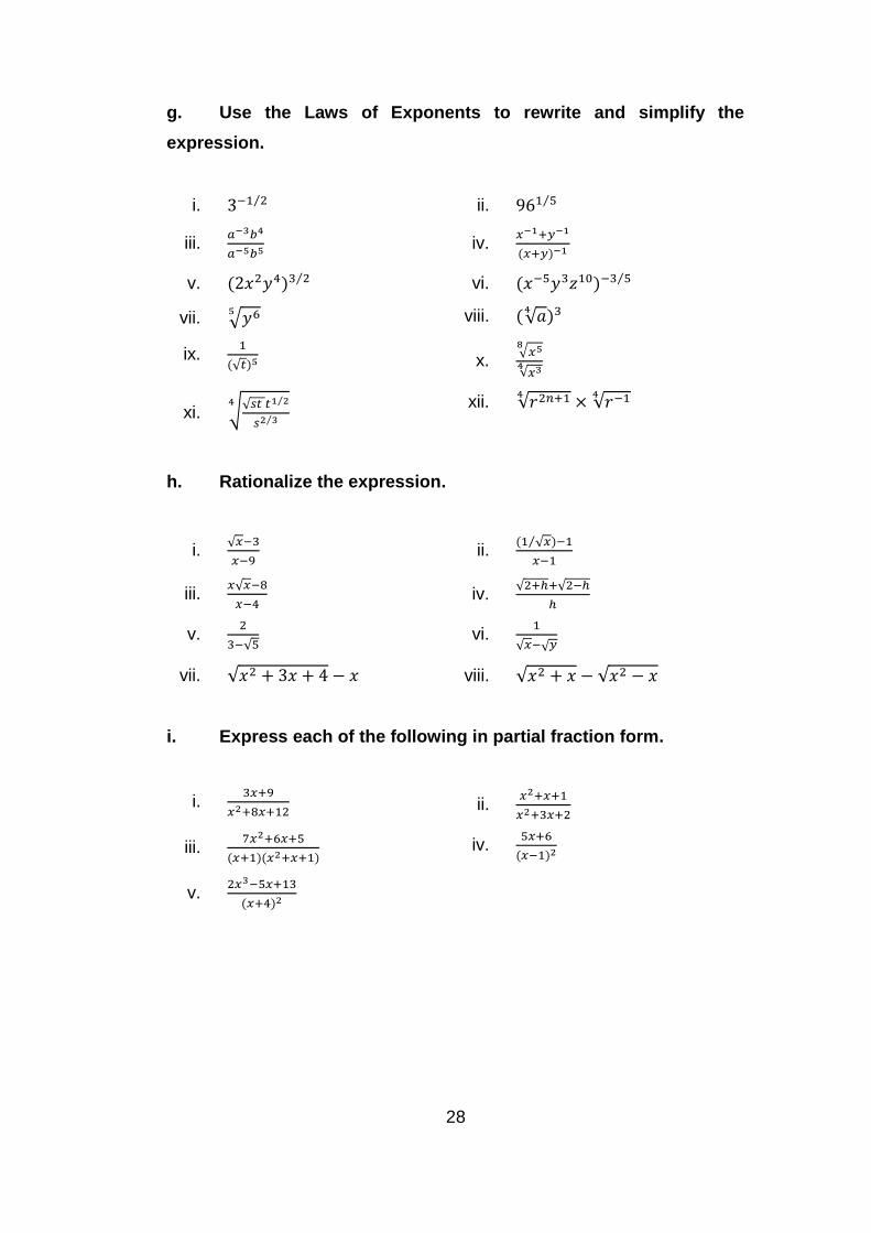
g. Use the Laws of Exponents to rewrite and simplify the

expression.

i. 3−1 2⁄ ii. 961 5⁄

iii. 𝑎−3𝑏4

𝑎−5𝑏5 iv.

𝑥−1+𝑦−1

(𝑥+𝑦)−1

v. (2𝑥2𝑦4)3 2⁄ vi. (𝑥−5𝑦3𝑧10)−3 5⁄

vii. √𝑦65 viii. (√𝑎

4)3

ix. 1

(√𝑡)5 x.

√𝑥58

√𝑥34

xi. √√𝑠𝑡 𝑡1 2⁄

𝑠2 3⁄

4

xii. √𝑟2𝑛+14

× √𝑟−14

h. Rationalize the expression.

i. √𝑥−3

𝑥−9 ii.

(1 √𝑥⁄ )−1

𝑥−1

iii. 𝑥√𝑥−8

𝑥−4 iv.

√2+ℎ+√2−ℎ

ℎ

v. 2

3−√5 vi.

1

√𝑥−√𝑦

vii. √𝑥2 + 3𝑥 + 4 − 𝑥 viii. √𝑥2 + 𝑥 − √𝑥2 − 𝑥

i. Express each of the following in partial fraction form.

i. 3𝑥+9

𝑥2+8𝑥+12 ii.

𝑥2+𝑥+1

𝑥2+3𝑥+2

iii. 7𝑥2+6𝑥+5

(𝑥+1)(𝑥2+𝑥+1) iv.

5𝑥+6

(𝑥−1)2

v. 2𝑥3−5𝑥+13

(𝑥+4)2