Revised Spring 2008

Santa Barbara City College

ENGR 101

Introduction To Engineering

Bookstore Packet

Nick Arnold

Table of Contents

ENGR 101, Introduction To Engineering, Bookstore Packet

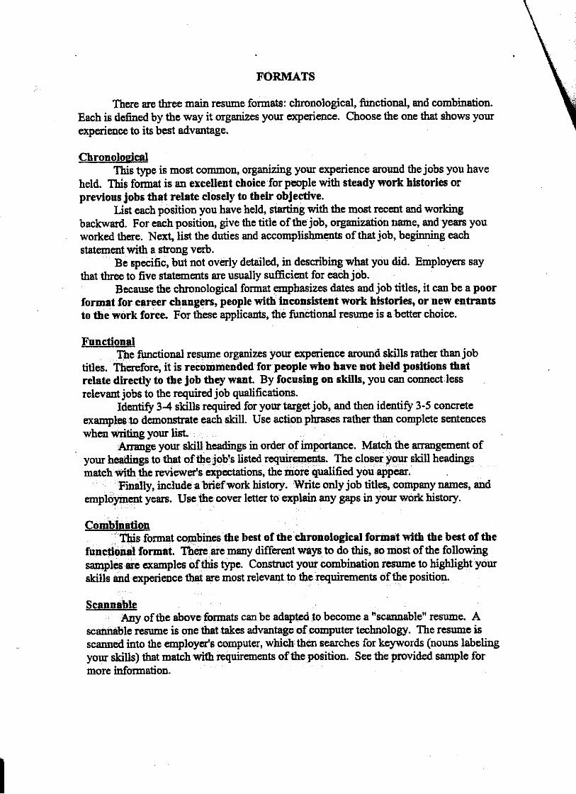
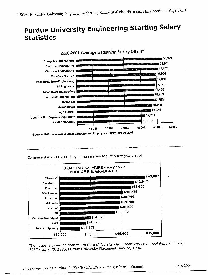
Preface: Important Information for Santa Barbara City College Students Majoring in Engineering SECTION 1: ENGINEERING PROFESSION Purdue University Engineering Starting Salary Statistics

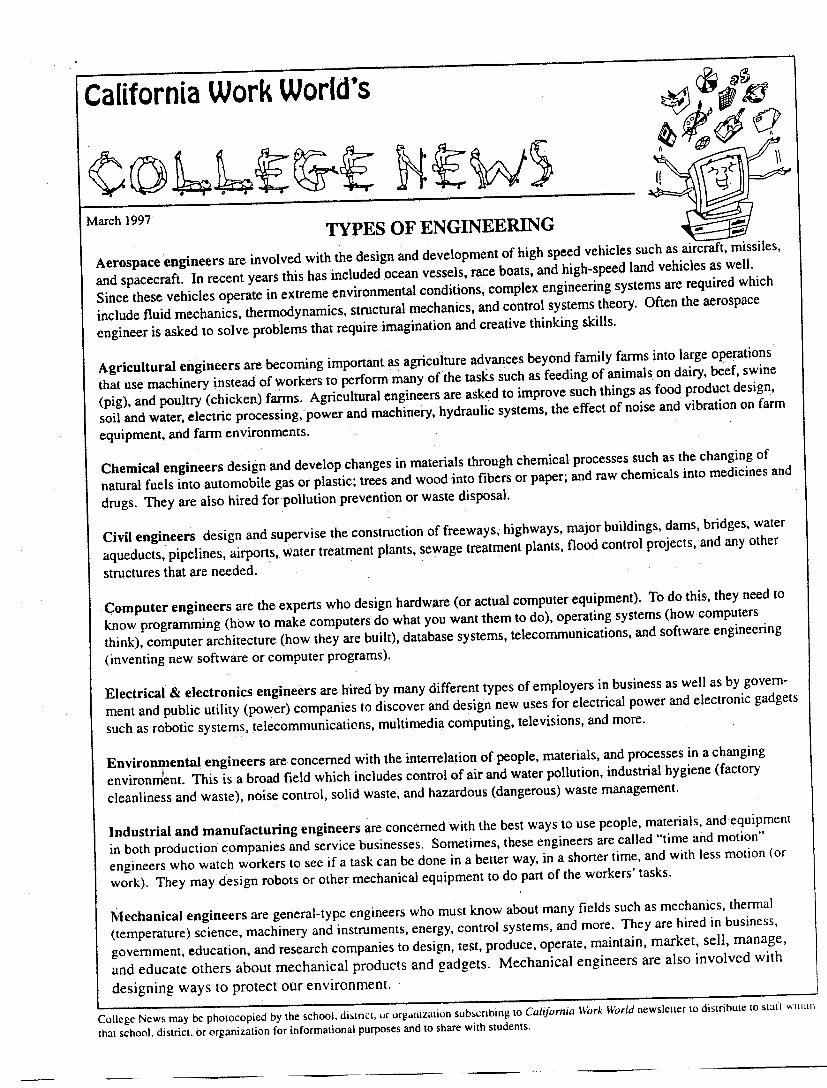
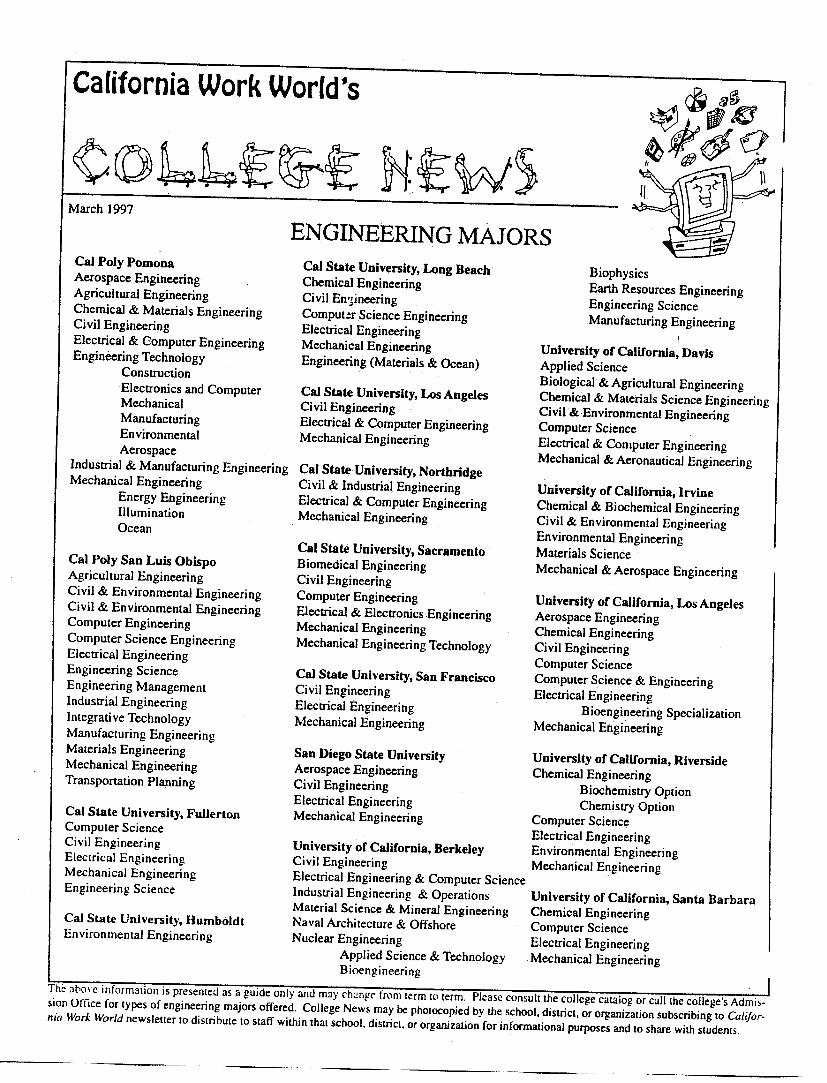
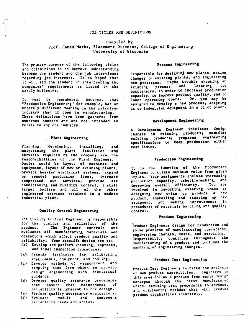
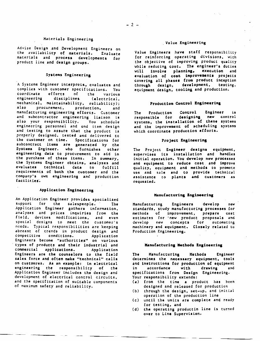
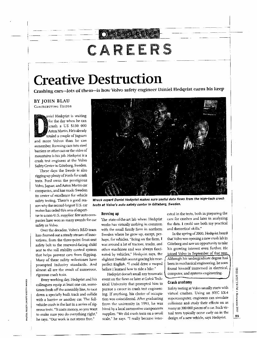
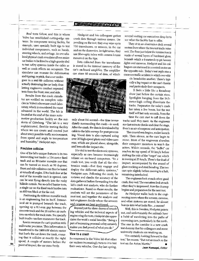
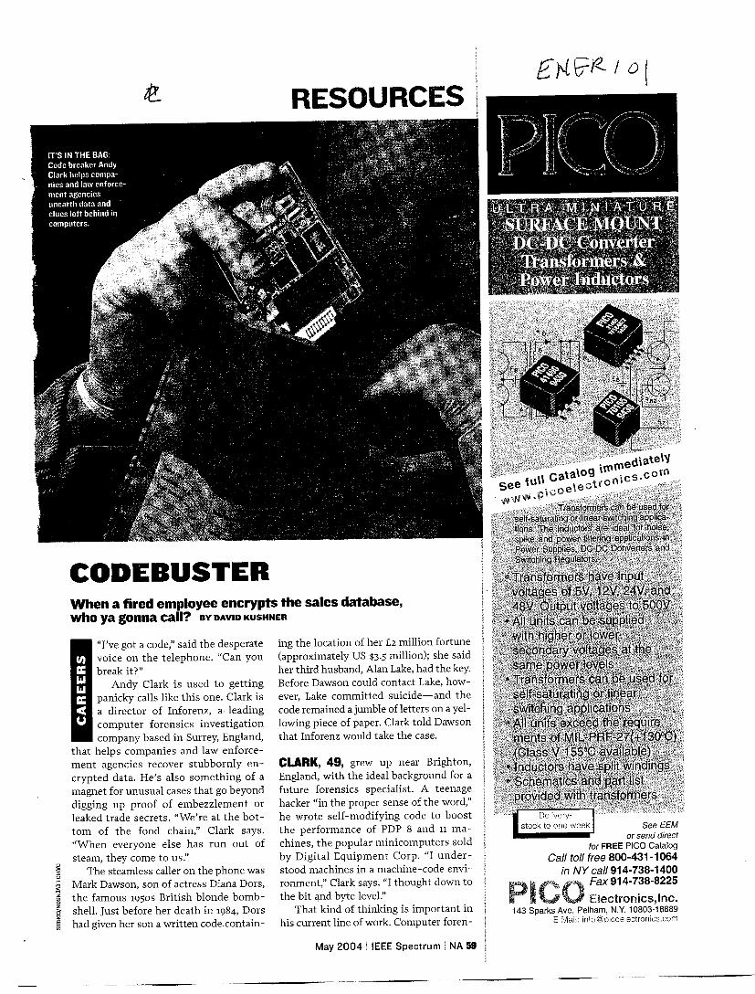
Types of Engineering Job Titles and Definitions Article, Creative Destruction Article, Code Buster

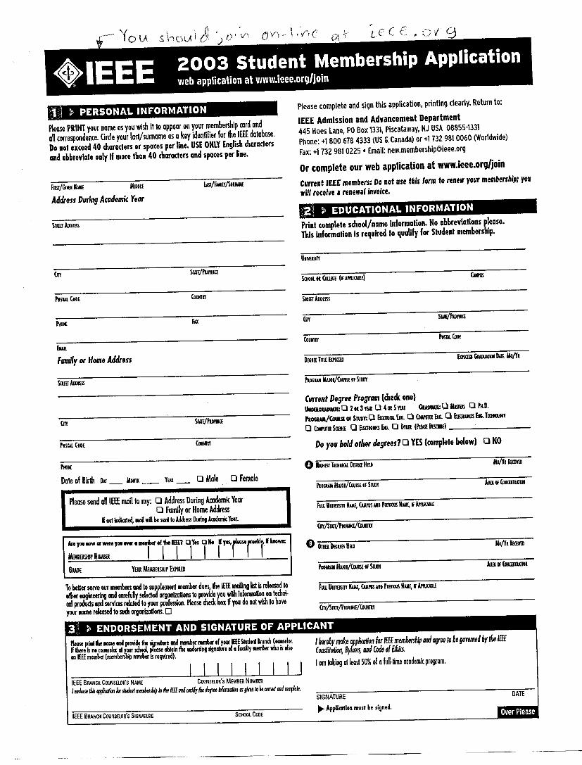
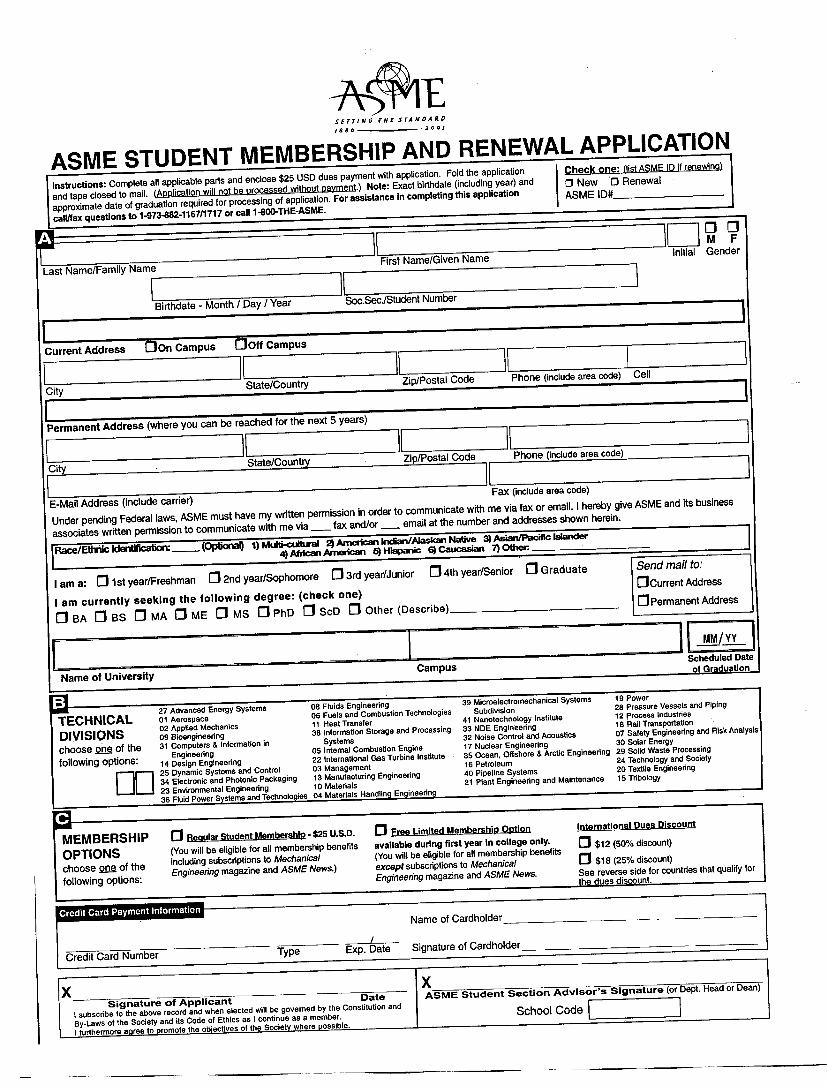
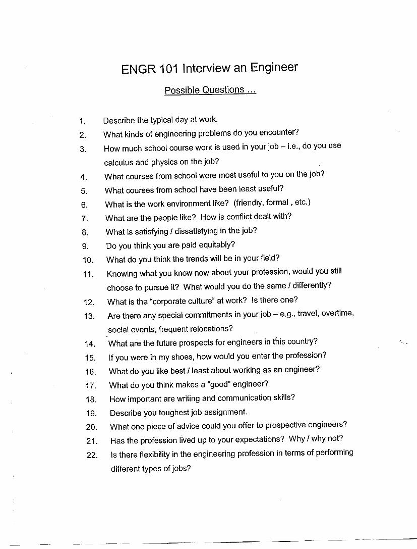
IEEE Membership Form (old, 2003, now you have to apply on-line) ASME Membership Form Interview an Engineer, Possible Questions

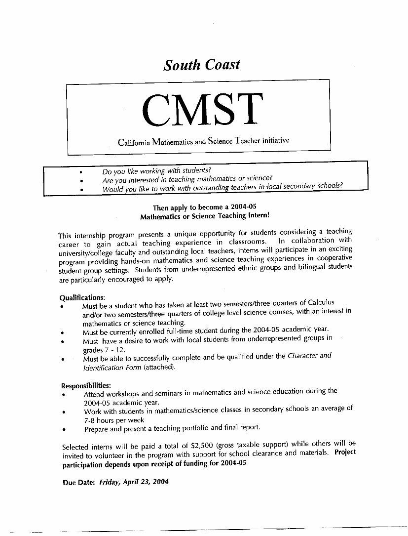
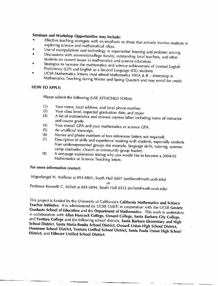
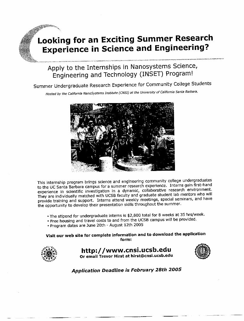
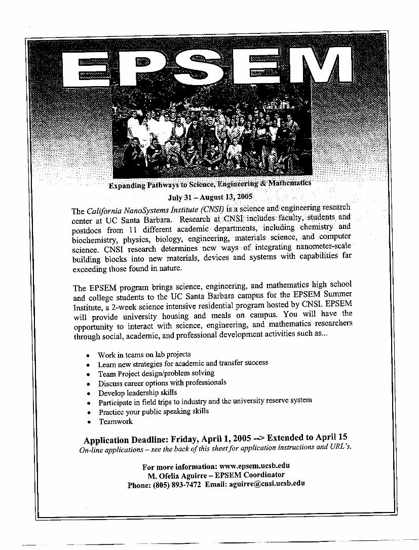
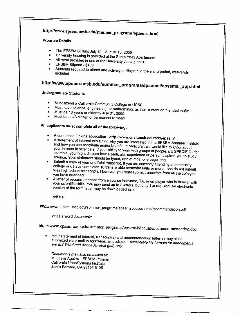
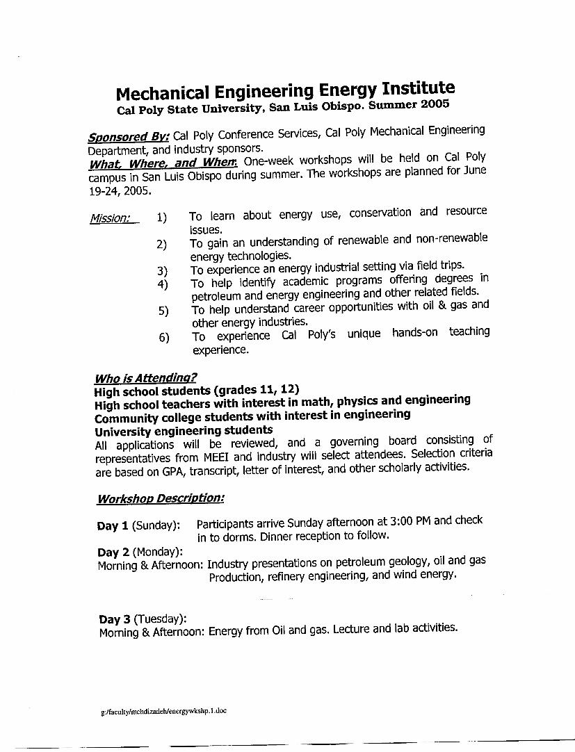
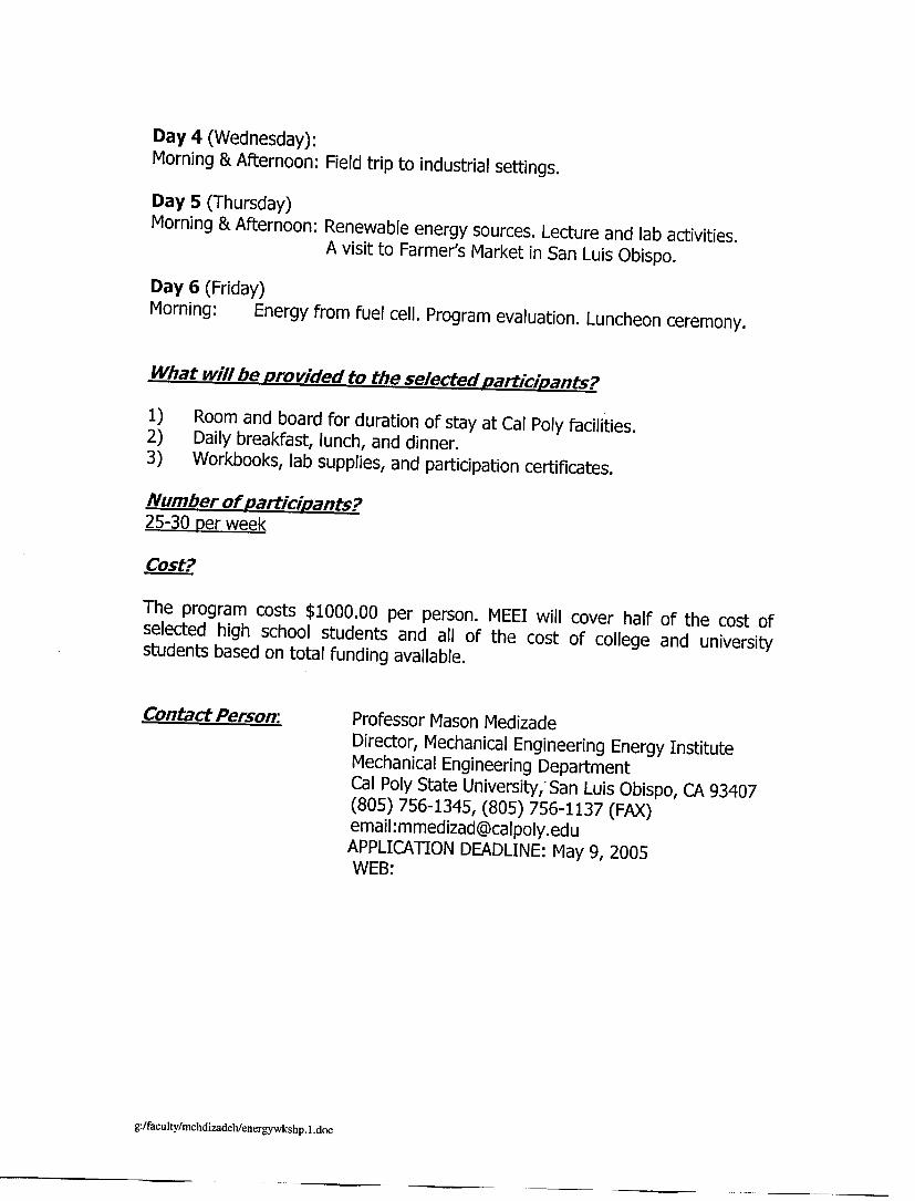
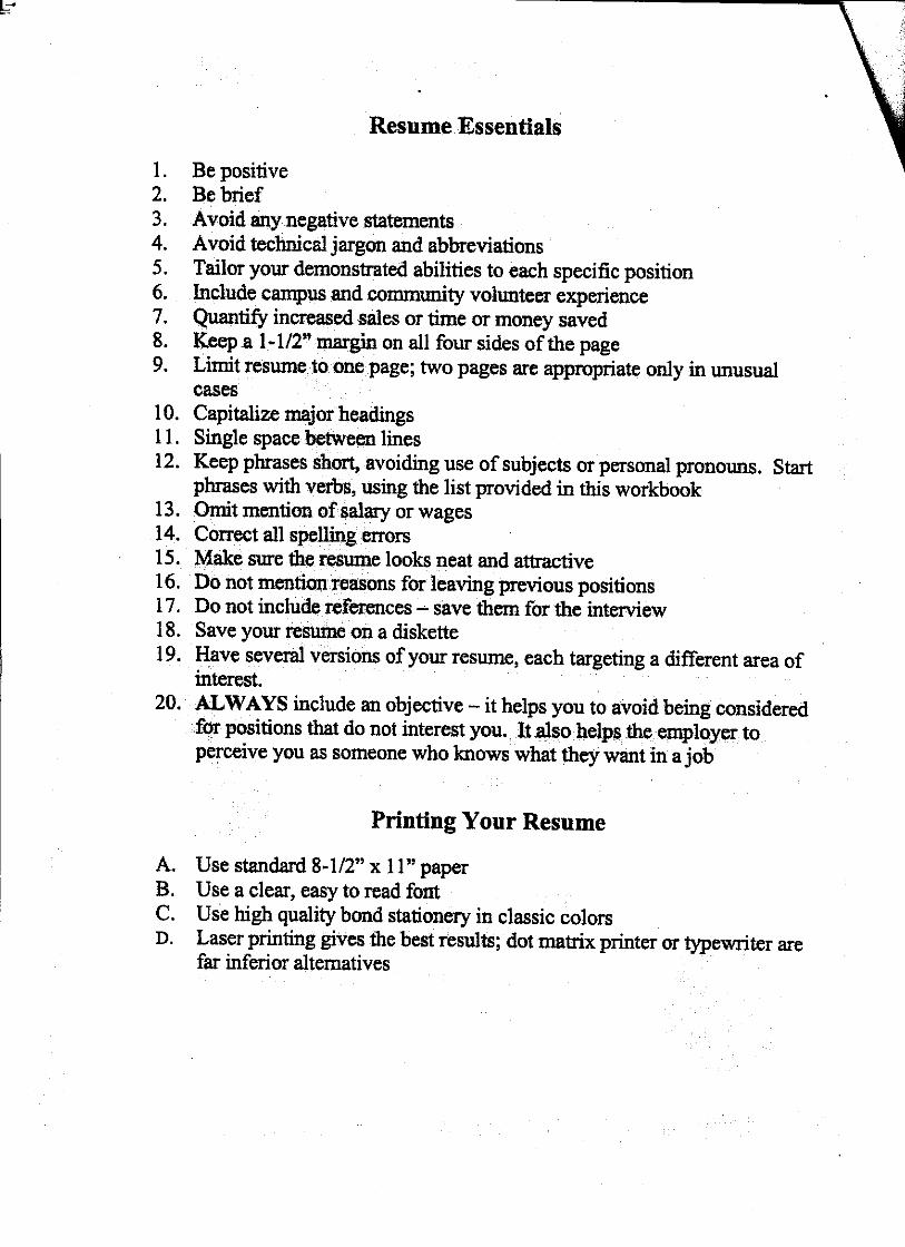
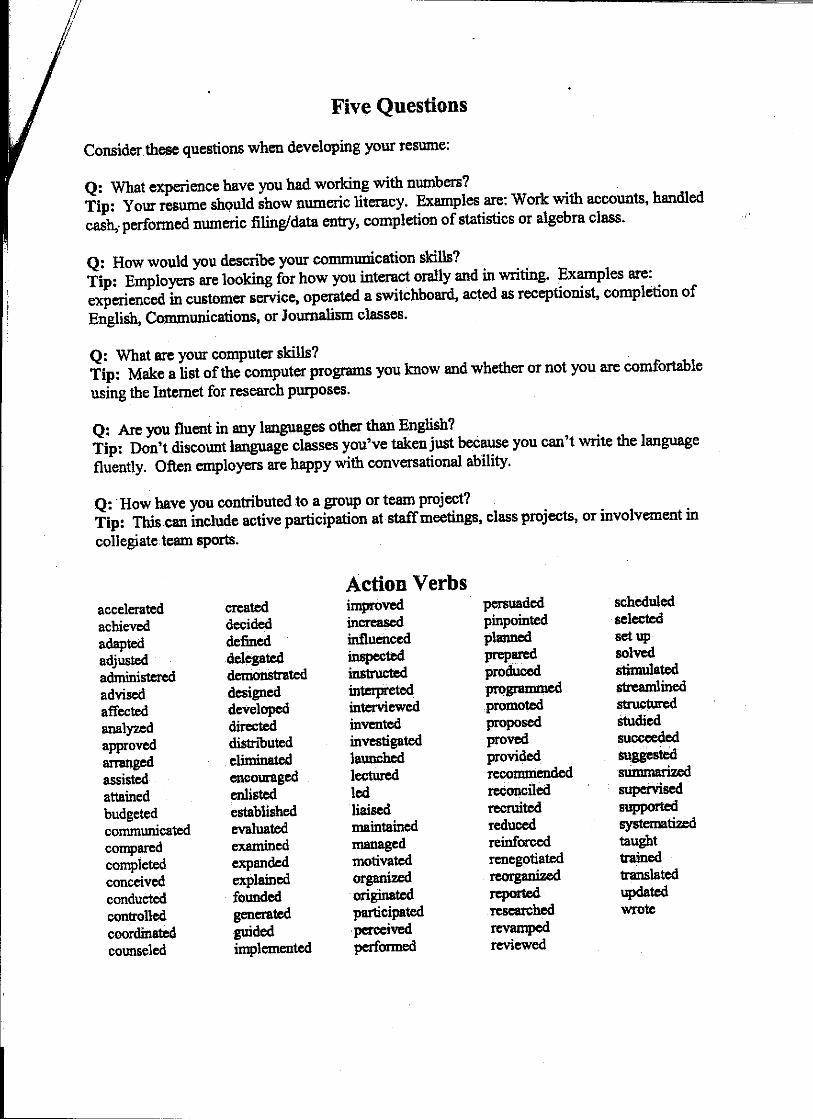
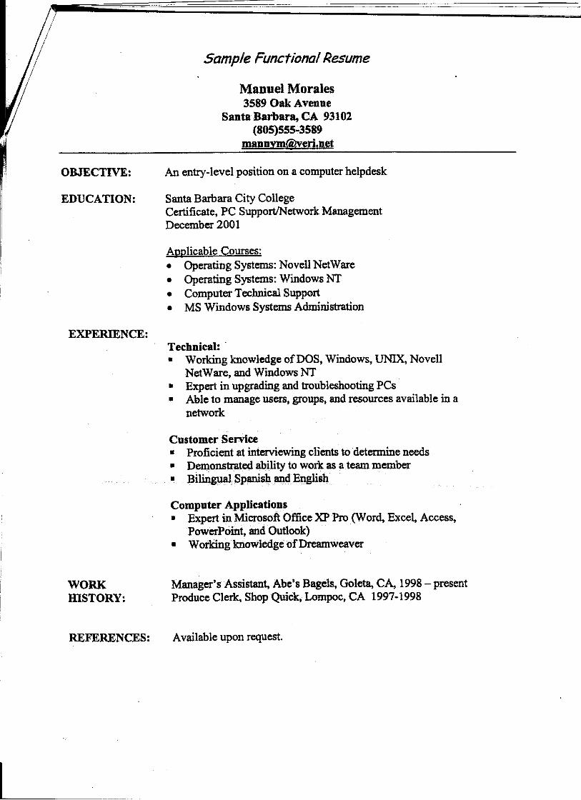
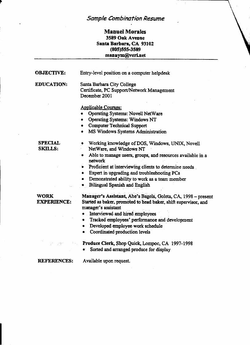
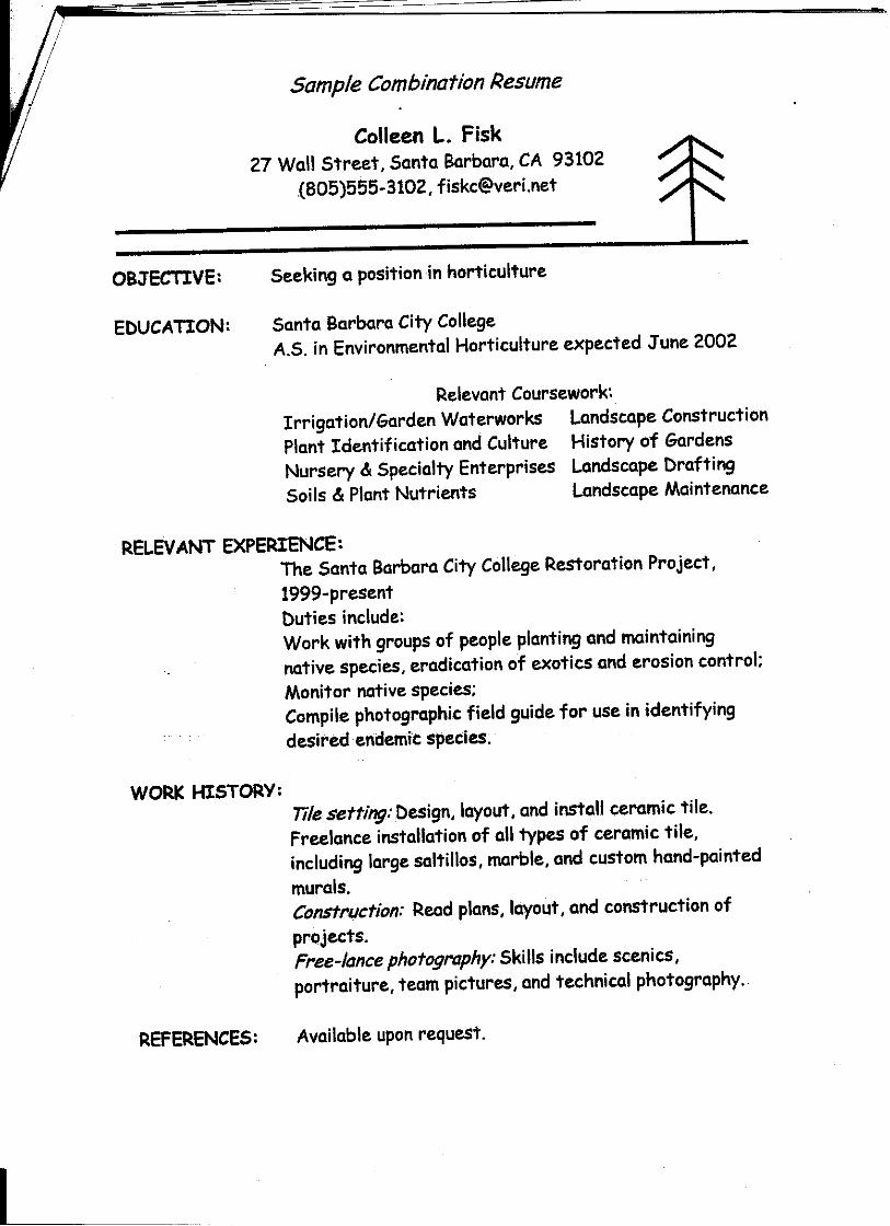
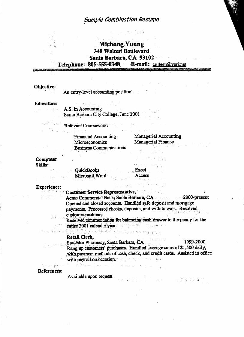
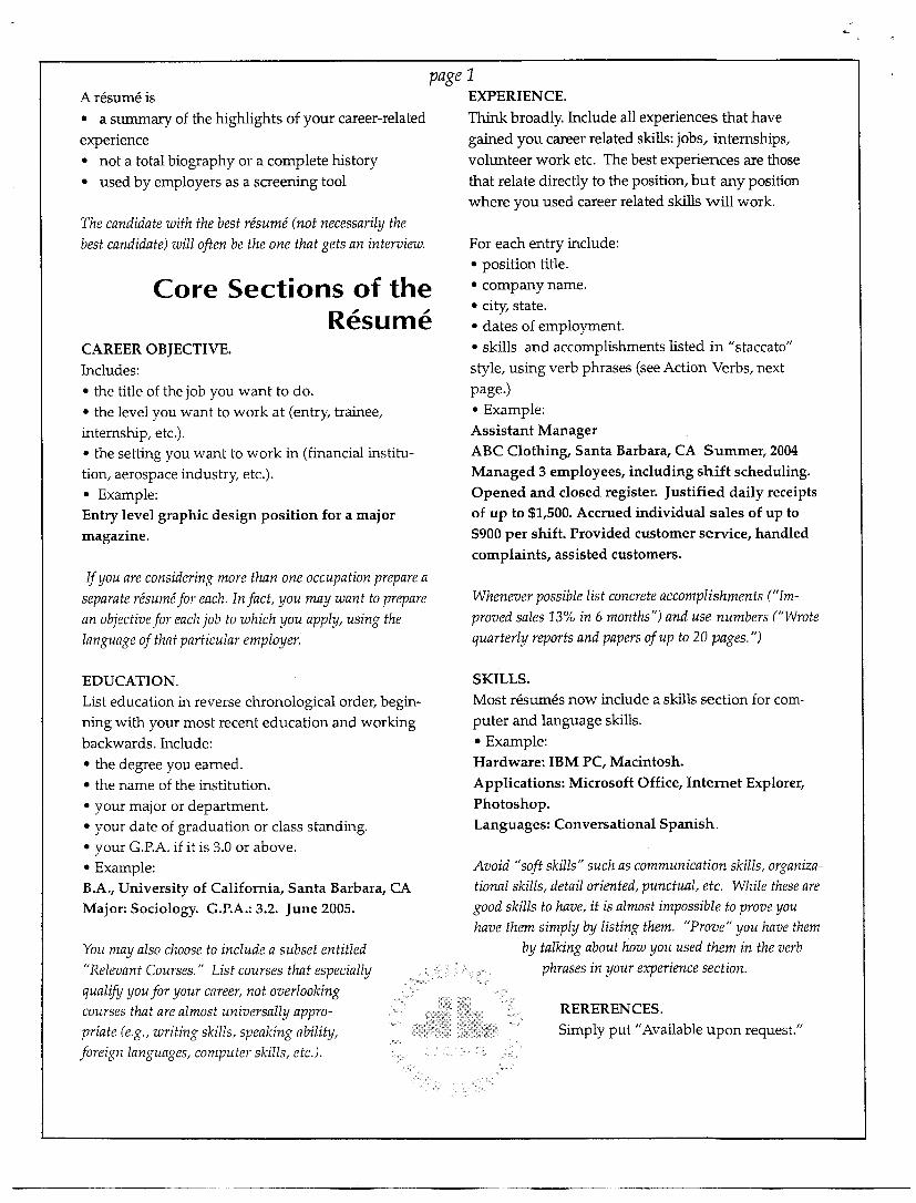
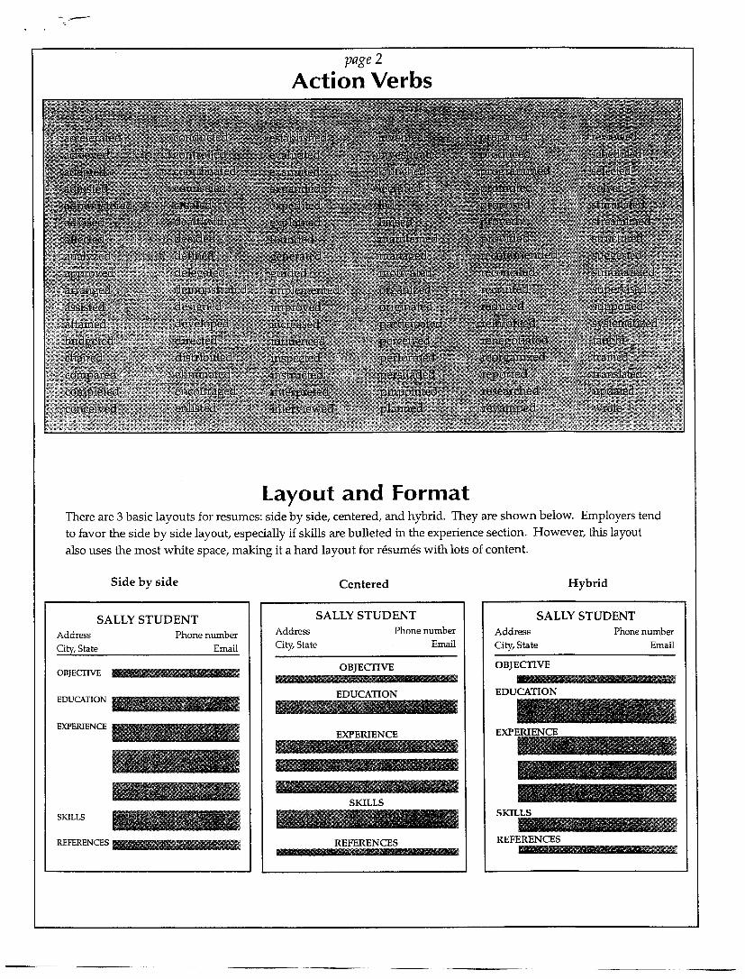
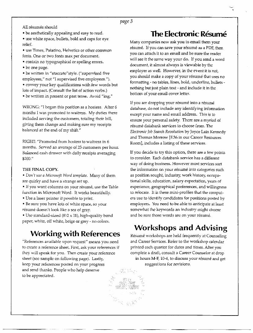
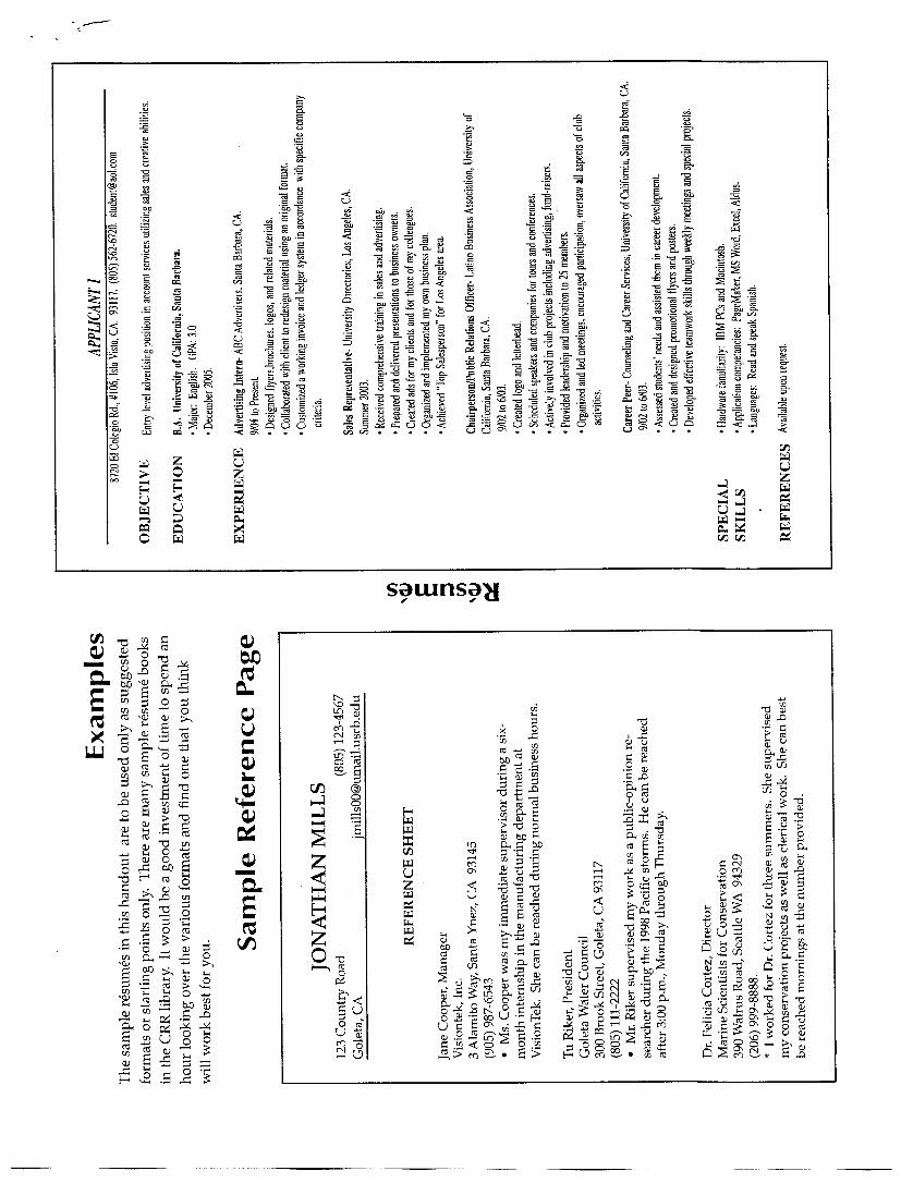
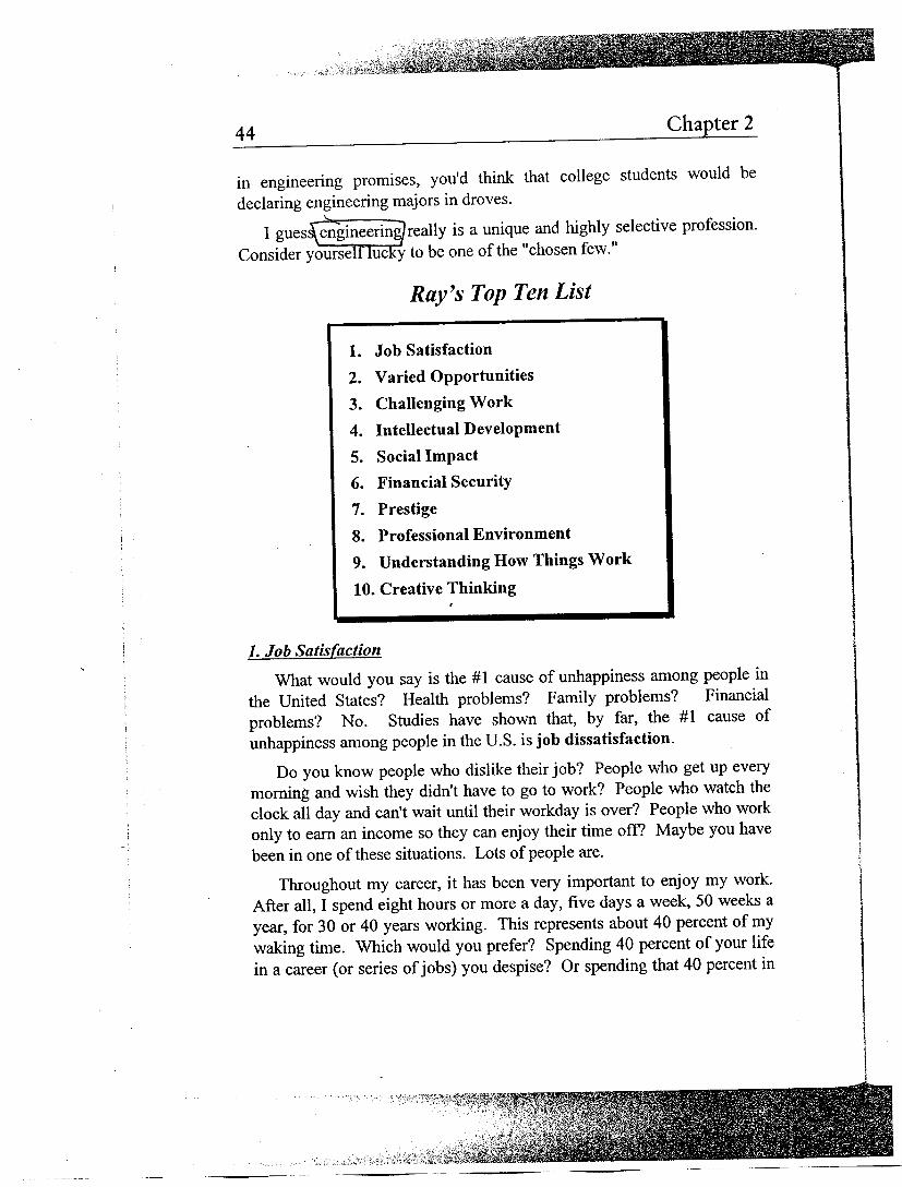
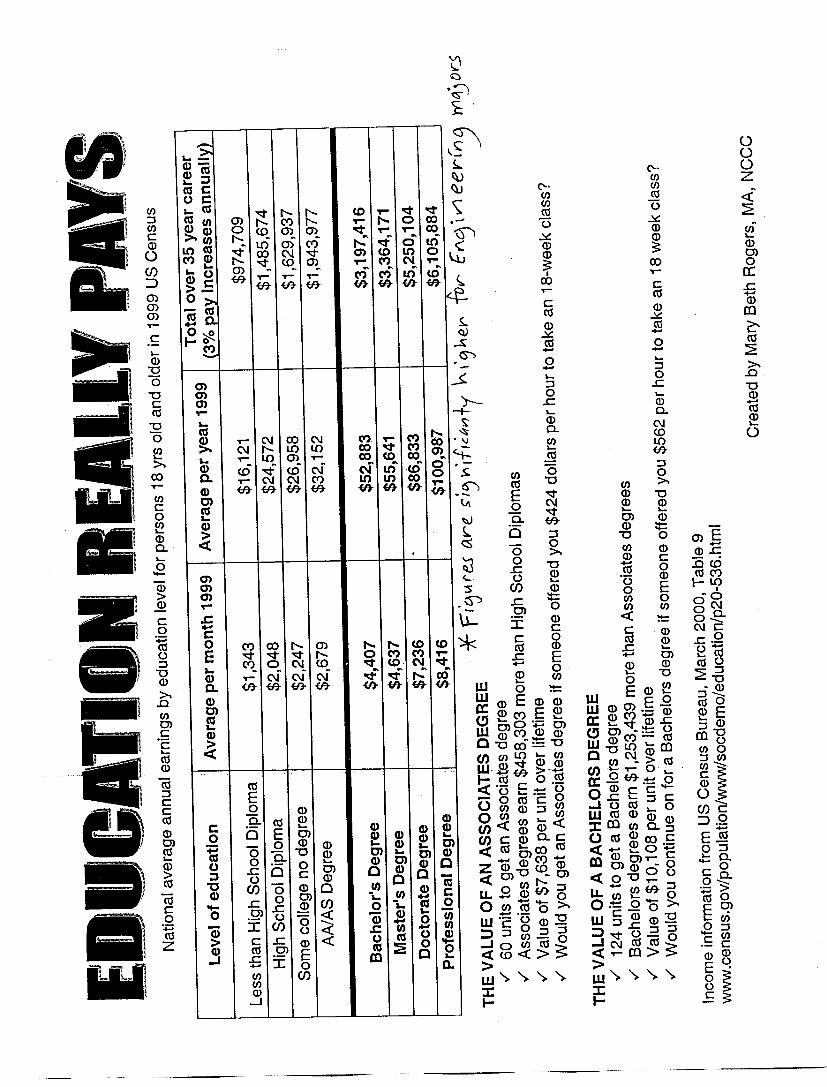
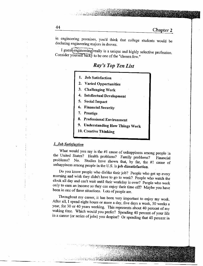
Ray’s Top Ten List SECTION 2: ENGINEERING ACADEMICS (* = not in this packet – to be handed out in class) “Education Really Pays” and “Ray’s Top Ten List” Helpful Hints & Hints for Taking a College Exam www.ASSIST.org Assignment for UCSB* www.ASSIST.org Assignment for Cal Poly and Others* IEP Assignment* SECTION 3: COMPUTER ASSIGNMENTS Excel Assignment #1: GPA Calculation Excel Assignment #2: Grade Calculation MatLab – Getting Started MatLab Assignment #1: M-files and Plotting MatLab Assignment #2: Random Roll of 1 Die and a Pair of Dice SECTION 4: INTERNSHIPS UCSB CMST Internship Info UCSB INSET Internship Info (see ENGR web site for other UC research internships for CC students) UCSB EPSEM Internship Info Seymour Duncan Internship Info Mechincal Engineering Energy Institute (MEEI) Internship Info, Cal Poly SECTION 5: APPENDIX The Resume Workbook, SBCC Career Center UCSB Resume Workbook

Important Information for Santa Barbara City College Students

Majoring in Engineering Who: * Santa Barbara City College Students Majoring in Engineering ! YOU! What: * Planning your personal schedule. * See a counselor – Maria Morales is one counselor who is very interested in helping

engineering students (the others in the “Engineering Cluster” are: Laura Castro, Wendy Peters, Sergio Perez & Shari Tucker).

* Visit the Transfer Center. * See Engineering Professor Nick Arnold to get up-to-date engineering program

information. * Go to www.ASSIST.org. When: * As Soon As Possible (ASAP)! * Especially while you can still add classes and change your schedule. Where: * Nick Arnold is in room ECC-10A (East Campus Classrooms) during his office hours,

or he can be reached at extension 4253, or email at arnold@sbcc.edu. * Maria Morales is in the counseling center, SS (Student Services) Bldg. * The Transfer Center is also in the SS (Student Services) Bldg. * www.ASSIST.org is on the internet. Why: * Taking the wrong classes, or taking classes in the wrong order can add years to the

time it takes you to complete your degree, and you could lose financial aid. * You may not be accepted for transfer without the proper courses, and some courses

need to be taken before you apply for transfer. * Learn about other strategies to ensure successful transfer. How: * Go to www.ASSIST.org. * Almost all engineering students should NOT do IGETC (Intersegmental General

Education Transfer Curriculum). * Talk to professors. * Talk to counselors. * Update and verify your IEP (Individual Education Plan) every semester. * Visit the Transfer Center. * Check the catalog and web pages of the schools you plan to apply to for transfer. * Talk to students who have transferred. * YOU are the one who is ultimately responsible for taking the right courses in the right

sequence and preparing yourself for transfer.

IGETC

Page 1 of 2

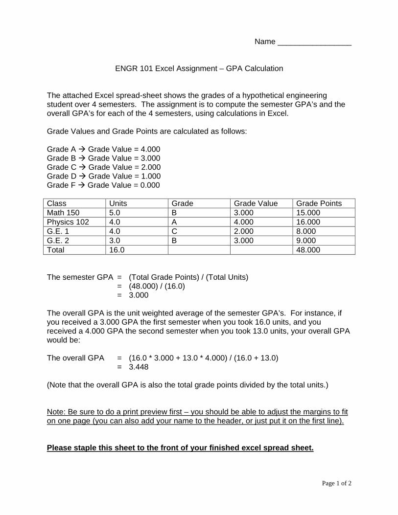
Name _________________

ENGR 101 Excel Assignment – GPA Calculation The attached Excel spread-sheet shows the grades of a hypothetical engineering student over 4 semesters. The assignment is to compute the semester GPA’s and the overall GPA’s for each of the 4 semesters, using calculations in Excel. Grade Values and Grade Points are calculated as follows: Grade A ! Grade Value = 4.000 Grade B ! Grade Value = 3.000 Grade C ! Grade Value = 2.000 Grade D ! Grade Value = 1.000 Grade F ! Grade Value = 0.000 Class Units Grade Grade Value Grade Points Math 150 5.0 B 3.000 15.000 Physics 102 4.0 A 4.000 16.000 G.E. 1 4.0 C 2.000 8.000 G.E. 2 3.0 B 3.000 9.000 Total 16.0 48.000 The semester GPA = (Total Grade Points) / (Total Units) = (48.000) / (16.0) = 3.000 The overall GPA is the unit weighted average of the semester GPA’s. For instance, if you received a 3.000 GPA the first semester when you took 16.0 units, and you received a 4.000 GPA the second semester when you took 13.0 units, your overall GPA would be: The overall GPA = (16.0 * 3.000 + 13.0 * 4.000) / (16.0 + 13.0) = 3.448 (Note that the overall GPA is also the total grade points divided by the total units.) Note: Be sure to do a print preview first – you should be able to adjust the margins to fit on one page (you can also add your name to the header, or just put it on the first line). Please staple this sheet to the front of your finished excel spread sheet.

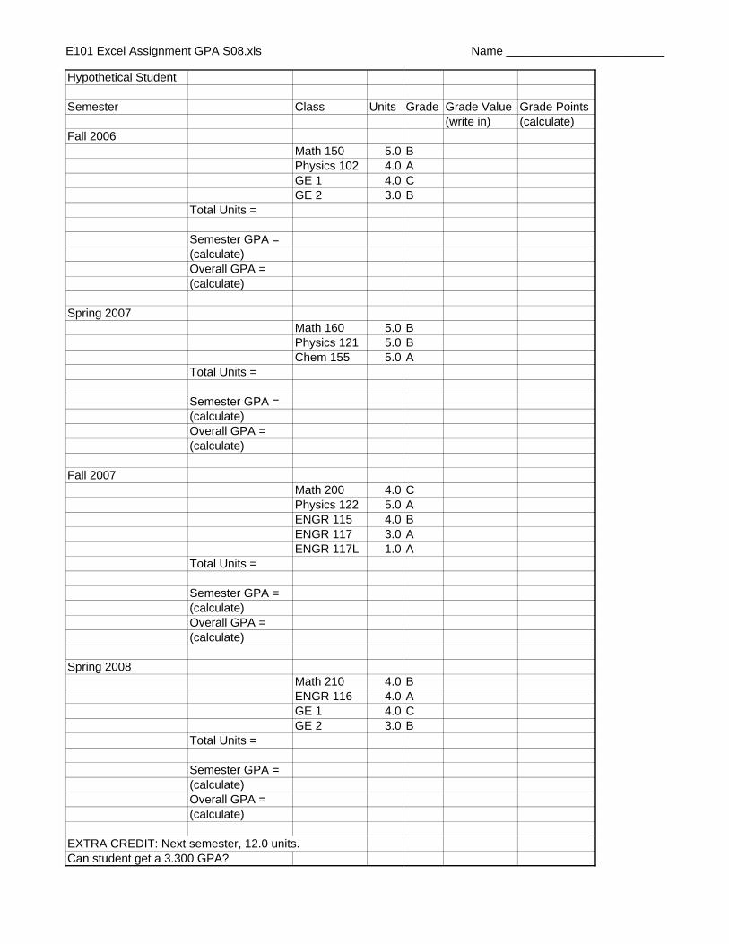
E101 Excel Assignment GPA S08.xls Name ________________________

Hypothetical Student

Semester Class Units Grade Grade Value Grade Points(write in) (calculate)

Fall 2006Math 150 5.0 BPhysics 102 4.0 AGE 1 4.0 CGE 2 3.0 B

Total Units =

Semester GPA = (calculate)Overall GPA = (calculate)

Spring 2007Math 160 5.0 BPhysics 121 5.0 BChem 155 5.0 A

Total Units =

Semester GPA = (calculate)Overall GPA = (calculate)

Fall 2007Math 200 4.0 CPhysics 122 5.0 AENGR 115 4.0 BENGR 117 3.0 AENGR 117L 1.0 A

Total Units =

Semester GPA = (calculate)Overall GPA = (calculate)

Spring 2008Math 210 4.0 BENGR 116 4.0 AGE 1 4.0 CGE 2 3.0 B

Total Units =

Semester GPA = (calculate)Overall GPA = (calculate)

EXTRA CREDIT: Next semester, 12.0 units.Can student get a 3.300 GPA?

Fall 2007

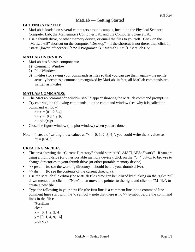
MatLab — Getting Started Page 1/2

MatLab — Getting Started GETTING STARTED: • MatLab is loaded on several computers around campus, including the Physical Sciences

Computer Lab, the Mathematics Computer Lab, and the Computer Science Lab. • Use a thumb drive, or other memory device, or email the files to yourself. Click on the

“MatLab 6.5” shortcut on the computer "Desktop" – if the shortcut is not there, then click on “start” (lower left corner) ! “All Programs” ! “MatLab 6.5” ! “MatLab 6.5”.

MATLAB OVERVIEW: • MatLab has 3 basic components:

1) Command Window 2) Plot Window 3) m-files (for saving your commands as files so that you can use them again – the m-file

actually becomes a command recognized by MatLab, in fact, all MatLab commands are written as m-files)

MATLAB COMMANDS: • The MatLab “command” window should appear showing the MatLab command prompt >> • Try entering the following commands into the command window (see why it is called the

command window): >> x = [0 1 2 3 4] >> y = [0 1 4 9 16] >> plot(x,y)

• Close the figure window (the plot window) when you are done. Note: Instead of writing the x-values as "x = [0, 1, 2, 3, 4]", you could write the x-values as

"x = [0:4]". CREATING M-FILES: • The area showing the “Current Directory” should start at “C:\MATLAB6p5\work”. If you are

using a thumb drive (or other portable memory device), click on the “…” button to browse to change directories to your thumb drive (or other portable memory device).

• >> pwd (to see the working directory – should be the your thumb drive). • >> dir (to see the contents of the current directory). • Use the MatLab file editor (the MatLab file editor can be utilized by clicking on the "File" pull

down menu, then click on "New", then move the pointer to the right and click on "M-file", to create a new file.

• Type the following in your new file (the first line is a comment line, not a command line – comment lines start with the % symbol – note that there is no >> symbol before the command lines in the file):

%test1.m clear x = [0, 1, 2, 3, 4] y = [0, 1, 4, 9, 16] plot(x,y)

Fall 2007

MatLab — Getting Started Page 2/2

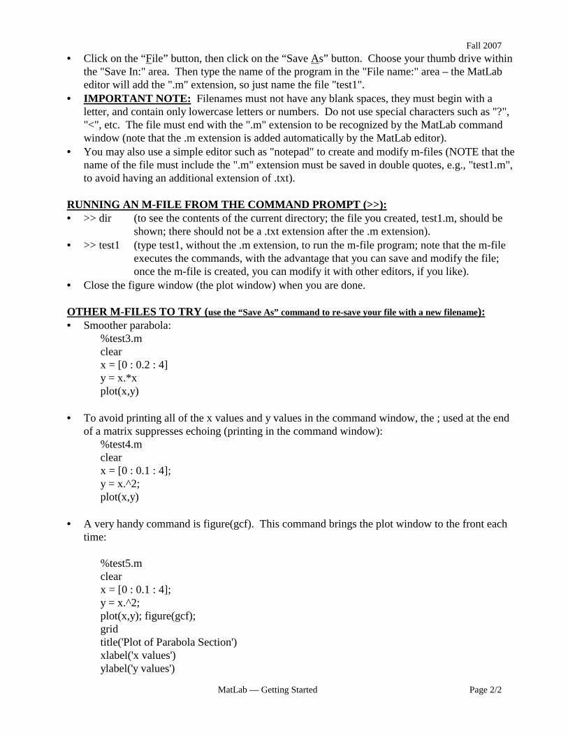
• Click on the “File” button, then click on the “Save As” button. Choose your thumb drive within the "Save In:" area. Then type the name of the program in the "File name:" area – the MatLab editor will add the ".m" extension, so just name the file "test1".

• IMPORTANT NOTE: Filenames must not have any blank spaces, they must begin with a letter, and contain only lowercase letters or numbers. Do not use special characters such as "?", "<", etc. The file must end with the ".m" extension to be recognized by the MatLab command window (note that the .m extension is added automatically by the MatLab editor).

• You may also use a simple editor such as "notepad" to create and modify m-files (NOTE that the name of the file must include the ".m" extension must be saved in double quotes, e.g., "test1.m", to avoid having an additional extension of .txt).

RUNNING AN M-FILE FROM THE COMMAND PROMPT (>>): • >> dir (to see the contents of the current directory; the file you created, test1.m, should be

shown; there should not be a .txt extension after the .m extension). • >> test1 (type test1, without the .m extension, to run the m-file program; note that the m-file

executes the commands, with the advantage that you can save and modify the file; once the m-file is created, you can modify it with other editors, if you like).

• Close the figure window (the plot window) when you are done. OTHER M-FILES TO TRY (use the “Save As” command to re-save your file with a new filename): • Smoother parabola:

%test3.m clear x = [0 : 0.2 : 4] y = x.*x plot(x,y)

• To avoid printing all of the x values and y values in the command window, the ; used at the end

of a matrix suppresses echoing (printing in the command window): %test4.m clear x = [0 : 0.1 : 4]; y = x.^2; plot(x,y)

• A very handy command is figure(gcf). This command brings the plot window to the front each

time:

%test5.m clear x = [0 : 0.1 : 4]; y = x.^2; plot(x,y); figure(gcf); grid title('Plot of Parabola Section') xlabel('x values') ylabel('y values')

Name ________________________________________

Page 1/1

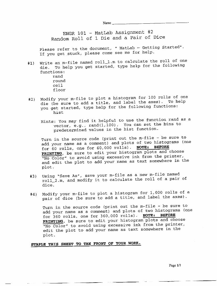
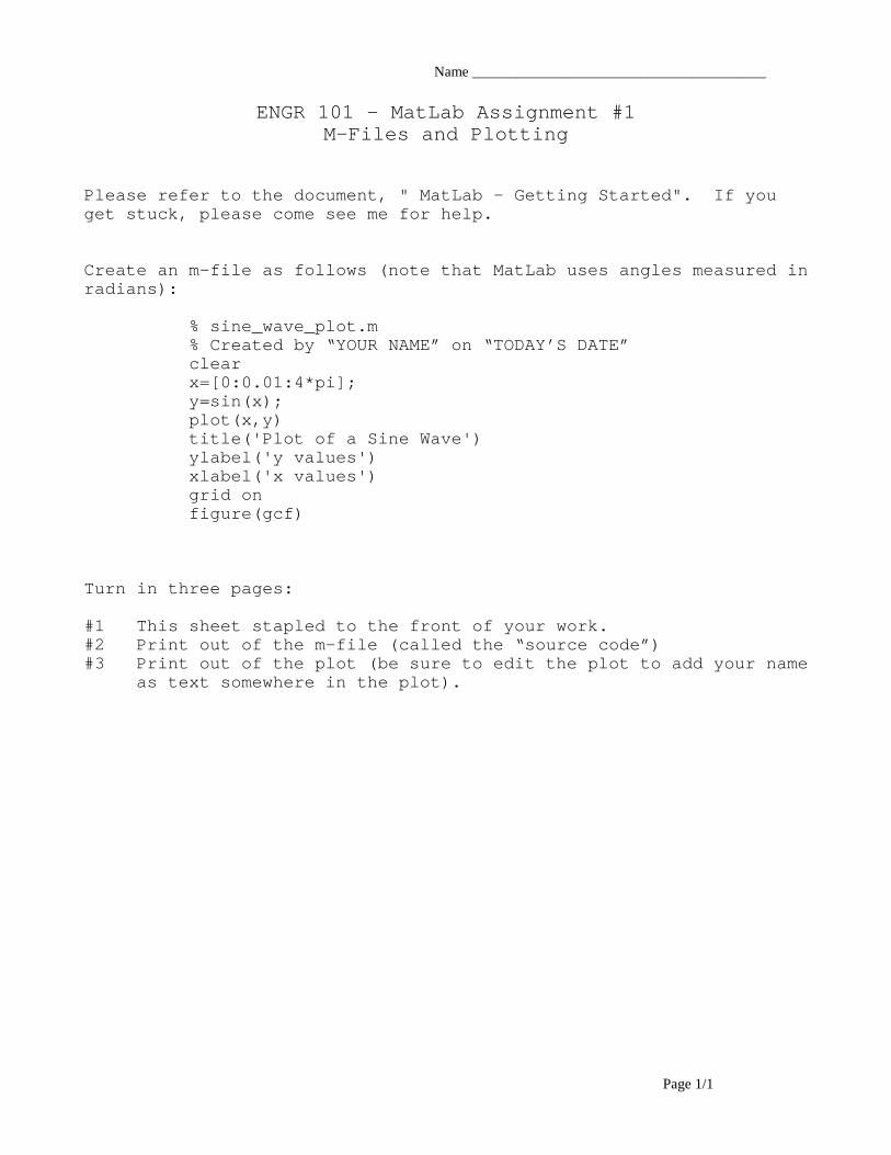
ENGR 101 – MatLab Assignment #1

M-Files and Plotting

Please refer to the document, " MatLab — Getting Started". If you get stuck, please come see me for help. Create an m-file as follows (note that MatLab uses angles measured in radians): % sine_wave_plot.m % Created by “YOUR NAME” on “TODAY’S DATE” clear

x=[0:0.01:4*pi]; y=sin(x); plot(x,y) title('Plot of a Sine Wave') ylabel('y values') xlabel('x values') grid on figure(gcf)

Turn in three pages: #1 This sheet stapled to the front of your work. #2 Print out of the m-file (called the “source code”) #3 Print out of the plot (be sure to edit the plot to add your name

as text somewhere in the plot).