Embed Size (px)
Citation preview
Revised Draft SGEIS 2011, Page 6-289
6.10 Noise 138
The noise impacts associated with horizontal drilling and high volume hydraulic fracturing are,
in general, similar to those addressed in the 1992 GEIS. The rigs and supporting equipment are
somewhat larger than the commonly used equipment described in 1992, but with the exception
of specialized downhole tools, horizontal drilling is performed using the same equipment,
technology, and procedures as used for many wells that have been drilled in New York.
Production-phase well site equipment is very quiet and has negligible impacts.
The greatest difference with respect to noise impacts, however, is in the duration of drilling. A
horizontal well takes four to five weeks of drilling at 24 hours per day to complete. The 1992
GEIS anticipated that most wells drilled in New York with rotary rigs would be completed in
less than one week, though drilling could extend two weeks or longer.
High-volume hydraulic fracturing is also of a larger scale than the water-gel fracs addressed in
1992. These were described as requiring 20,000 to 80,000 gallons of water pumped into the well
at pressures of 2,000 to 3,500 pounds per square inch (psi). High-volume hydraulic fracturing of
a typical horizontal well could require, on average, 3.6 million gallons of water and a maximum
pumping pressure that may be as high as 10,000 to 11,000 psi. This volume and pressure would
result in more pump and fluid handling noise than anticipated in 1992. The proposed process
requires three to five days to complete. There was no mention of the time required for hydraulic
fracturing in 1992.
There would also be significantly more trucking and associated noise involved with high-volume
hydraulic fracturing than was addressed in the 1992 GEIS.
Site preparation, drilling, and hydraulic fracturing activities could result in temporary noise
impacts, depending on the distance from the site to the nearest noise-sensitive receptors.
Typically, the following factors are considered when evaluating a construction noise impact:
138 Section 6.10, in its entirety, was provided by Ecology and Environment Engineering, P.C., August 2011, and was adapted by
the Department.
Revised Draft SGEIS 2011, Page 6-290
Difference between existing noise levels prior to construction startup and expected noise
levels during construction;
Absolute level of expected construction noise;
Adjacent land uses; and
The duration of construction activity.
In order to evaluate the potential noise impacts related to the drilling operation phases, a
construction noise model was used to estimate noise levels at various distances from the
construction site during a typical hour for each phase of construction. The algorithm in the
model considered construction equipment noise specification data, usage factors, and distance.
The following logarithmic equation was used to compute projected noise levels:
Lp1 = Lp2 + 10log(U.F./10) – 20log(d2/d1):
where:
Lp1 = the average noise level (dBA) at a distance (d2) due to the operation of a unit of
equipment throughout the day;
Lp2 = the equipment noise level (dBA) at a reference distance (d1);
U.F. = a usage factor that accounts for a fraction of time an equipment unit is in use
throughout the day;
d2 = the distance from the unit of equipment in feet; and
d1 = the distance at which equipment noise level data is known.
Noise levels and usage factor data for construction equipment were obtained from industry
sources and government publications. Usage factors were used to account for the fact that
construction equipment use is intermittent throughout the course of a normal workday.
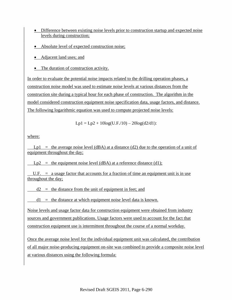
Once the average noise level for the individual equipment unit was calculated, the contribution
of all major noise-producing equipment on-site was combined to provide a composite noise level
at various distances using the following formula:
Revised Draft SGEIS 2011, Page 6-291
Using this approach, the estimated noise levels are conservative in that they do not take into
consideration any noise reduction due to ground attenuation, atmospheric absorption,
topography, or vegetation.
6.10.1 Access Road Construction
Newly constructed access roads are typically unpaved and are generally 20 to 40 feet wide
during the construction phase and 10 to 20 feet wide during the production phase. They are
constructed to efficiently provide access to the well pad while minimizing potential
environmental impacts.
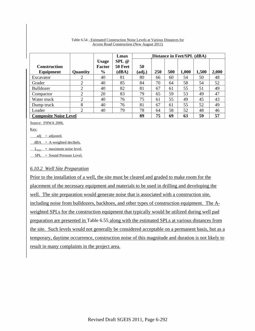
The estimated sound pressure levels (SPLs) produced by construction equipment that would be
used to build or improve access roads are presented in Table 6.54 for various distances. The
composite result is derived by assuming that all of the construction equipment listed in the table
is operating at the percent utilization time listed and by combining their SPLs logarithmically.
These SPLs might temporarily occur over the course of access road construction. Such levels
would not generally be considered acceptable on a permanent basis, but as a temporary, daytime
occurrence, construction noise of this magnitude and duration is not likely to result in many
complaints in the project area.
....101010log10 101010
321
etcLeq
LeqLeqLeq
total
Revised Draft SGEIS 2011, Page 6-292
Table 6.54 - Estimated Construction Noise Levels at Various Distances for
Access Road Construction (New August 2011)
Construction
Equipment Quantity
Usage
Factor
%
Lmax
SPL @
50 Feet
(dBA)
Distance in Feet/SPL (dBA)
50
(adj.) 250 500 1,000 1,500 2,000
Excavator 2 40 81 80 66 60 54 50 48
Grader 2 40 85 84 70 64 58 54 52
Bulldozer 2 40 82 81 67 61 55 51 49
Compactor 2 20 83 79 65 59 53 49 47
Water truck 2 40 76 75 61 55 49 45 43
Dump truck 8 40 76 81 67 61 55 52 49
Loader 2 40 79 78 64 58 52 48 46
Composite Noise Level 89 75 69 63 59 57
Source: FHWA 2006.
Key:
adj = adjusted.
dBA = A-weighted decibels.
Lmax = maximum noise level.
SPL = Sound Pressure Level.
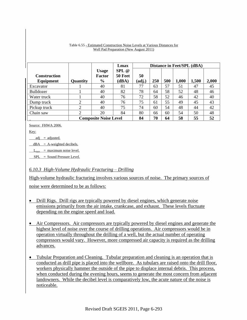
6.10.2 Well Site Preparation
Prior to the installation of a well, the site must be cleared and graded to make room for the
placement of the necessary equipment and materials to be used in drilling and developing the
well. The site preparation would generate noise that is associated with a construction site,
including noise from bulldozers, backhoes, and other types of construction equipment. The A-
weighted SPLs for the construction equipment that typically would be utilized during well pad
preparation are presented in Table 6.55 along with the estimated SPLs at various distances from
the site. Such levels would not generally be considered acceptable on a permanent basis, but as a
temporary, daytime occurrence, construction noise of this magnitude and duration is not likely to
result in many complaints in the project area.
Revised Draft SGEIS 2011, Page 6-293
Table 6.55 - Estimated Construction Noise Levels at Various Distances for
Well Pad Preparation (New August 2011)
Construction
Equipment Quantity
Usage
Factor
%
Lmax
SPL @
50 Feet
(dBA)
Distance in Feet/SPL (dBA)
50
(adj.) 250 500 1,000 1,500 2,000
Excavator 1 40 81 77 63 57 51 47 45
Bulldozer 1 40 82 78 64 58 52 48 46
Water truck 1 40 76 72 58 52 46 42 40
Dump truck 2 40 76 75 61 55 49 45 43
Pickup truck 2 40 75 74 60 54 48 44 42
Chain saw 2 20 84 80 66 60 54 50 48
Composite Noise Level 84 70 64 58 55 52
Source: FHWA 2006.
Key:
adj = adjusted.
dBA = A-weighted decibels.
Lmax = maximum noise level.
SPL = Sound Pressure Level.
6.10.3 High-Volume Hydraulic Fracturing – Drilling
High-volume hydraulic fracturing involves various sources of noise. The primary sources of
noise were determined to be as follows:
Drill Rigs. Drill rigs are typically powered by diesel engines, which generate noise
emissions primarily from the air intake, crankcase, and exhaust. These levels fluctuate
depending on the engine speed and load.
Air Compressors. Air compressors are typically powered by diesel engines and generate the
highest level of noise over the course of drilling operations. Air compressors would be in
operation virtually throughout the drilling of a well, but the actual number of operating
compressors would vary. However, more compressed air capacity is required as the drilling
advances.
Tubular Preparation and Cleaning. Tubular preparation and cleaning is an operation that is
conducted as drill pipe is placed into the wellbore. As tubulars are raised onto the drill floor,
workers physically hammer the outside of the pipe to displace internal debris. This process,
when conducted during the evening hours, seems to generate the most concern from adjacent
landowners. While the decibel level is comparatively low, the acute nature of the noise is
noticeable.
Revised Draft SGEIS 2011, Page 6-294
Elevator Operation. Elevators are used to move drill pipe and casing into and/or out of the
wellbore. During drilling, elevators are used to add additional pipe to the drill string as the
depth increases. Elevators are used when the operator is removing multiple sections of pipe
from the well or placing drill pipe or casing into the wellbore. Elevator operation is not a
constant activity and its duration is dependent on the depth of the well bore. The decibel
level is low.
Drill Pipe Connections. As the depth of the well increases, the operator must connect
additional pipe to the drill string. Most operators in the Appalachian Basins use a method
known as ―air-drilling.‖ As the drill bit penetrates the rock the cuttings must be removed
from the wellbore. Cuttings are removed by displacing pressurized air (from the air
compressors discussed above) into the well bore. As the air is circulated back to the surface,
it carries with it the rock cuttings. To connect additional pipe to the drill string, the operator
will release the air pressure. It is the release of pressure that creates a higher frequency noise
impact.
Once initiated, the drilling operation often continues 24 hours a day until completion and would
therefore generate noise during nighttime hours, when people are generally involved in activities
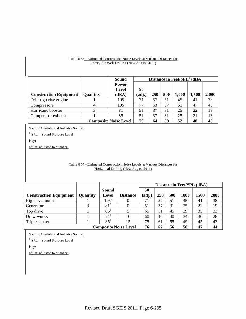
that require lower ambient noise levels. Certain noise-producing equipment is typically operated
on a fairly continuous basis during the drilling process. The types and quantities of this
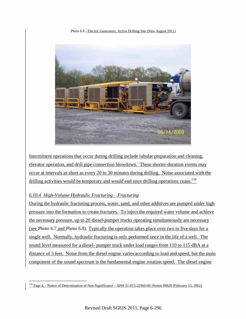
equipment are presented in Table 6.56 for rotary air drilling and in Table 6.57 for horizontal
drilling (see Photo 6.6), along with the estimated A-weighted individual and composite SPLs that
would be experienced at various distances from the operation. An analysis of both types of
drilling is included since according to industry sources, in accessing the natural gas formation,
rotary air drilling is often used for the vertical section of the well and then horizontal drilling is
used for making the turn and completing the horizontal section.
Revised Draft SGEIS 2011, Page 6-295
Table 6.56 - Estimated Construction Noise Levels at Various Distances for
Rotary Air Well Drilling (New August 2011)
Construction Equipment Quantity
Sound
Power
Level
(dBA)
Distance in Feet/SPL1 (dBA)
50
(adj.) 250 500 1,000 1,500 2,000
Drill rig drive engine 1 105 71 57 51 45 41 38
Compressors 4 105 77 63 57 51 47 45
Hurricane booster 3 81 51 37 31 25 22 19
Compressor exhaust 1 85 51 37 31 25 21 18
Composite Noise Level 79 64 58 52 48 45
Source: Confidential Industry Source.
1 SPL = Sound Pressure Level
Key:
adj = adjusted to quantity.
Table 6.57 - Estimated Construction Noise Levels at Various Distances for
Horizontal Drilling (New August 2011)
Construction Equipment Quantity
Sound
Level Distance
Distance in Feet/SPL (dBA)
50
(adj.) 250 500 1000 1500 2000
Rig drive motor 1 1052 0 71 57 51 45 41 38
Generator 3 812 0 51 37 31 25 22 19
Top drive 1 851 5 65 51 45 39 35 33
Draw works 1 741 10 60 46 40 34 30 28
Triple shaker 1 851 15 75 61 55 49 45 43
Composite Noise Level 76 62 56 50 47 44
Source: Confidential Industry Source.
1 SPL = Sound Pressure Level
Key:
adj = adjusted to quantity.
Revised Draft SGEIS 2011, Page 6-296
Photo 6.6 - Electric Generators, Active Drilling Site (New August 2011)
Intermittent operations that occur during drilling include tubular preparation and cleaning,
elevator operation, and drill pipe connection blowdown. These shorter-duration events may
occur at intervals as short as every 20 to 30 minutes during drilling. Noise associated with the
drilling activities would be temporary and would end once drilling operations cease.139
6.10.4 High-Volume Hydraulic Fracturing – Fracturing
During the hydraulic fracturing process, water, sand, and other additives are pumped under high
pressure into the formation to create fractures. To inject the required water volume and achieve
the necessary pressure, up to 20 diesel-pumper trucks operating simultaneously are necessary
(see Photo 6.7 and Photo 6.8). Typically the operation takes place over two to five days for a
single well. Normally, hydraulic fracturing is only performed once in the life of a well. The
sound level measured for a diesel- pumper truck under load ranges from 110 to 115 dBA at a
distance of 3 feet. Noise from the diesel engine varies according to load and speed, but the main
component of the sound spectrum is the fundamental engine rotation speed. The diesel engine
139 Page 4, - Notice of Determination of Non-Significance – API# 31-015-22960-00, Permit 08828 (February 13, 2002)
Revised Draft SGEIS 2011, Page 6-297
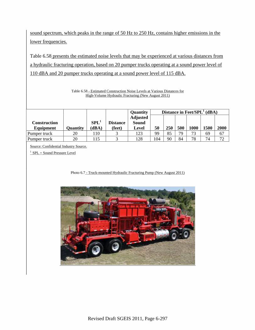
sound spectrum, which peaks in the range of 50 Hz to 250 Hz, contains higher emissions in the
lower frequencies.
Table 6.58 presents the estimated noise levels that may be experienced at various distances from
a hydraulic fracturing operation, based on 20 pumper trucks operating at a sound power level of
110 dBA and 20 pumper trucks operating at a sound power level of 115 dBA.
Table 6.58 - Estimated Construction Noise Levels at Various Distances for
High-Volume Hydraulic Fracturing (New August 2011)
Construction
Equipment Quantity
SPL1
(dBA)
Distance
(feet)
Quantity
Adjusted
Sound
Level
Distance in Feet/SPL1 (dBA)
50 250 500 1000 1500 2000
Pumper truck 20 110 3 123 99 85 79 73 69 67
Pumper truck 20 115 3 128 104 90 84 78 74 72
Source: Confidential Industry Source.
1 SPL = Sound Pressure Level
Photo 6.7 - Truck-mounted Hydraulic Fracturing Pump (New August 2011)
Revised Draft SGEIS 2011, Page 6-298
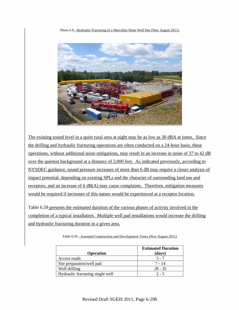
Photo 6.8 - Hydraulic Fracturing of a Marcellus Shale Well Site (New August 2011)
The existing sound level in a quiet rural area at night may be as low as 30 dBA at times. Since
the drilling and hydraulic fracturing operations are often conducted on a 24-hour basis, these
operations, without additional noise mitigations, may result in an increase in noise of 37 to 42 dB
over the quietest background at a distance of 2,000 feet. As indicated previously, according to
NYSDEC guidance, sound pressure increases of more than 6 dB may require a closer analysis of
impact potential, depending on existing SPLs and the character of surrounding land use and
receptors, and an increase of 6 dB(A) may cause complaints. Therefore, mitigation measures
would be required if increases of this nature would be experienced at a receptor location.
Table 6.59 presents the estimated duration of the various phases of activity involved in the
completion of a typical installation. Multiple well pad installations would increase the drilling
and hydraulic fracturing duration in a given area.
Table 6.59 - Assumed Construction and Development Times (New August 2011)
Operation
Estimated Duration
(days)
Access roads 3 - 7
Site preparation/well pad 7 - 14
Well drilling 28 - 35
Hydraulic fracturing single well 2 - 5
Revised Draft SGEIS 2011, Page 6-299
6.10.5 Transportation
Similar to any construction operation, drill sites require the use of support equipment and
vehicles. Specialized cement equipment and vehicles, water trucks, flatbed tractor trailers, and
delivery and employee vehicles are the most common forms of support machinery and vehicles.
Cement equipment would generate additional noise during operations, but this impact is typically
short lived and is at levels below that of the compressors described above.
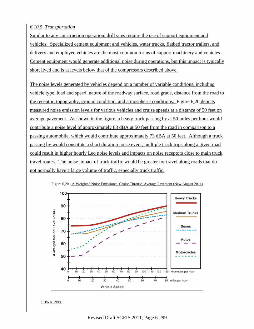
The noise levels generated by vehicles depend on a number of variable conditions, including
vehicle type, load and speed, nature of the roadway surface, road grade, distance from the road to
the receptor, topography, ground condition, and atmospheric conditions. Figure 6.20 depicts
measured noise emission levels for various vehicles and cruise speeds at a distance of 50 feet on
average pavement. As shown in the figure, a heavy truck passing by at 50 miles per hour would
contribute a noise level of approximately 83 dBA at 50 feet from the road in comparison to a
passing automobile, which would contribute approximately 73 dBA at 50 feet. Although a truck
passing by would constitute a short duration noise event, multiple truck trips along a given road
could result in higher hourly Leq noise levels and impacts on noise receptors close to main truck
travel routes. The noise impact of truck traffic would be greater for travel along roads that do
not normally have a large volume of traffic, especially truck traffic.
Figure 6.20 - A-Weighted Noise Emissions: Cruise Throttle, Average Pavement (New August 2011)
FHWA 1998.
Revised Draft SGEIS 2011, Page 6-300
In addition to the trucks required to deliver the drill rig and its associated equipment, trucks are
used to bring in water for drilling and hydraulic fracturing, sand for hydraulic fracturing additive,
and frac tanks. Trucks are also used for the removal of flowback for the site. Estimates of truck
trips per well and truck trips over time during the early development phase of a horizontal and a
vertical well installation are presented in Section 6.11, Transportation.
Development of multiple wells on a single pad would add substantial additional truck traffic
volume in an area, which would be at least partially offset by a reduction in the number of well
pads overall.
This level of truck traffic could have negative noise impacts on those living in proximity to the
well site and access road. Like other noise associated with drilling, this would be temporary.
Current regulations require that all wells on a multi-well pad be drilled within three years of
starting the first well. Thus, it is possible that someone living in proximity to the pad would
experience adverse noise impacts intermittently for up to three years.
6.10.6 Gas Well Production
Once the well has been completed and the equipment has been demobilized, the pad is partially
reclaimed. The remaining wellhead production does not generate a significant level of noise.
Operation and maintenance activities could include a truck visit to empty the condensate
collection tanks on an approximately weekly basis, but condensate production from the
Marcellus Shale in New York is not typically expected. Mowing of the well pad area occurs
approximately two times per year. These activities would result in infrequent, short-term noise
events.
6.11 Transportation Impacts140
While the trucking for site preparation, rig, equipment, materials, and supplies is similar for
horizontal drilling to what was anticipated in 1992, the water requirement of high–volume
hydraulic fracturing could lead to significantly more truck traffic than was discussed in the GEIS
in the regions where natural gas development would occur. This section presents (1) industry
140 Section 6.11, in its entirety, was provided by Ecology and Environment Engineering, P.C., August 2011, and was adapted by
the Department.
Revised Draft SGEIS 2011, Page 6-301
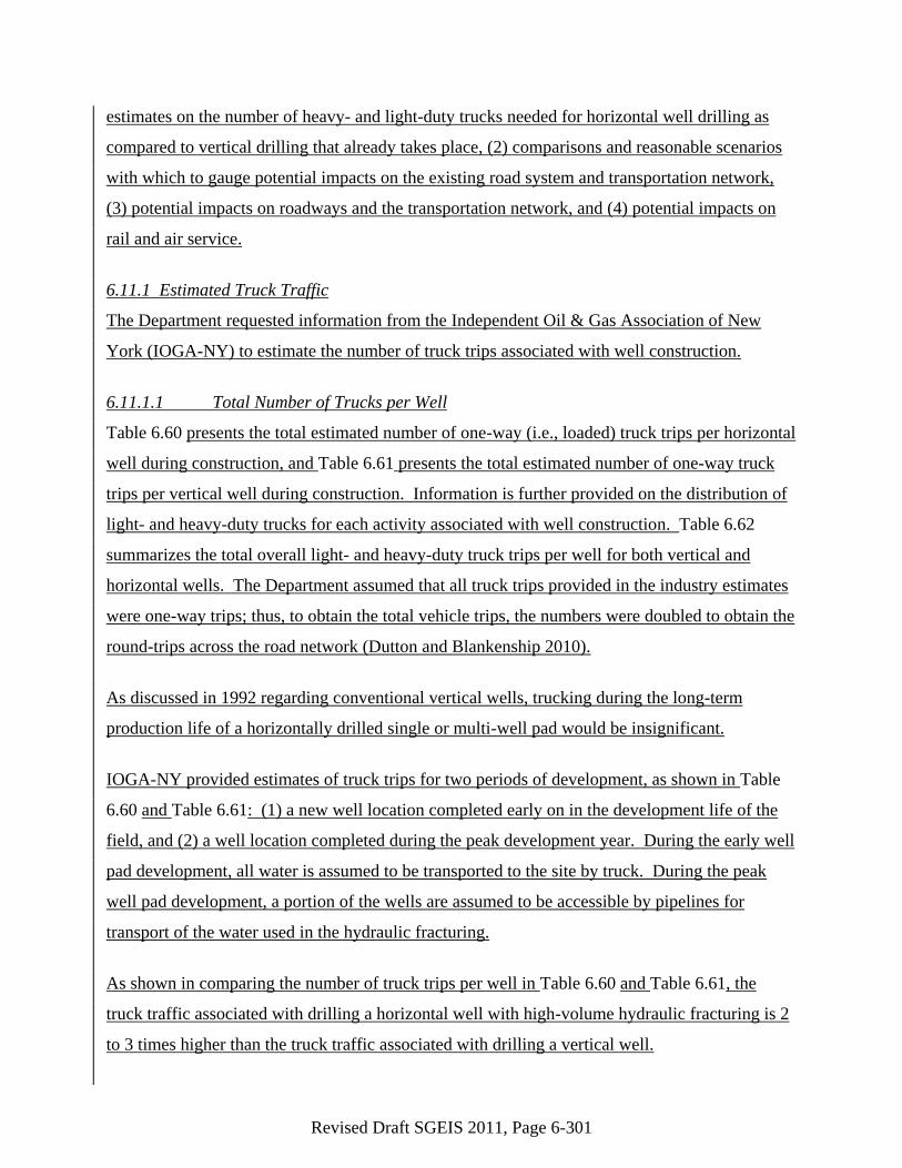
estimates on the number of heavy- and light-duty trucks needed for horizontal well drilling as
compared to vertical drilling that already takes place, (2) comparisons and reasonable scenarios
with which to gauge potential impacts on the existing road system and transportation network,
(3) potential impacts on roadways and the transportation network, and (4) potential impacts on
rail and air service.
6.11.1 Estimated Truck Traffic
The Department requested information from the Independent Oil & Gas Association of New
York (IOGA-NY) to estimate the number of truck trips associated with well construction.
6.11.1.1 Total Number of Trucks per Well
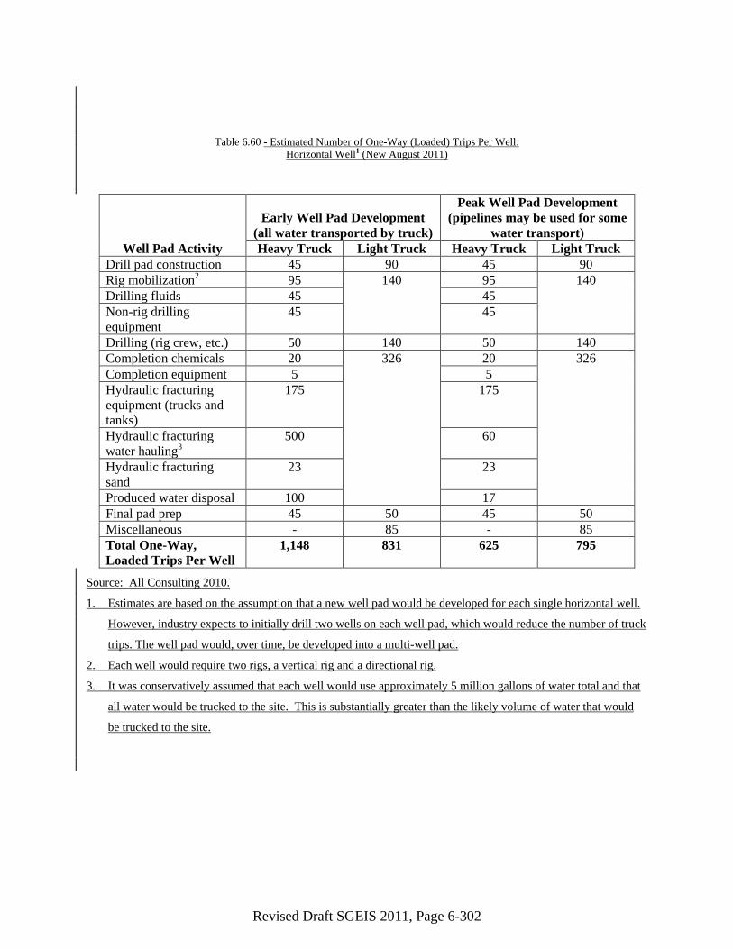
Table 6.60 presents the total estimated number of one-way (i.e., loaded) truck trips per horizontal
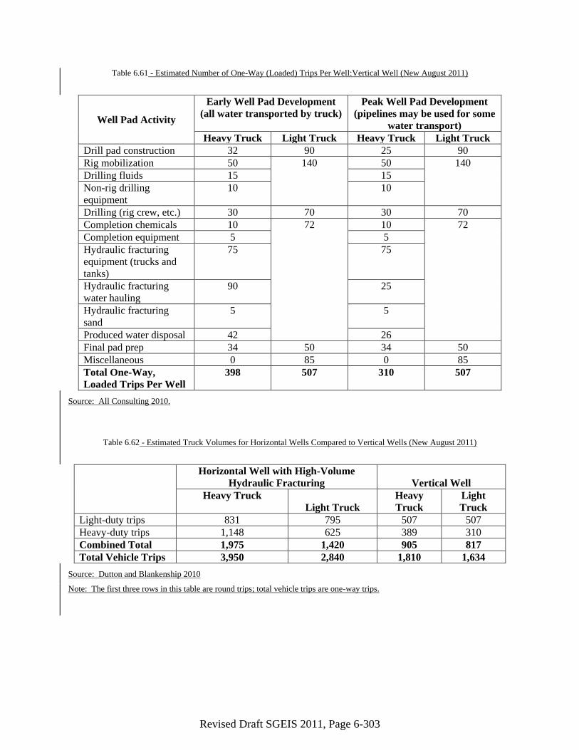
well during construction, and Table 6.61 presents the total estimated number of one-way truck
trips per vertical well during construction. Information is further provided on the distribution of
light- and heavy-duty trucks for each activity associated with well construction. Table 6.62
summarizes the total overall light- and heavy-duty truck trips per well for both vertical and
horizontal wells. The Department assumed that all truck trips provided in the industry estimates
were one-way trips; thus, to obtain the total vehicle trips, the numbers were doubled to obtain the
round-trips across the road network (Dutton and Blankenship 2010).
As discussed in 1992 regarding conventional vertical wells, trucking during the long-term
production life of a horizontally drilled single or multi-well pad would be insignificant.
IOGA-NY provided estimates of truck trips for two periods of development, as shown in Table
6.60 and Table 6.61: (1) a new well location completed early on in the development life of the
field, and (2) a well location completed during the peak development year. During the early well
pad development, all water is assumed to be transported to the site by truck. During the peak
well pad development, a portion of the wells are assumed to be accessible by pipelines for
transport of the water used in the hydraulic fracturing.
As shown in comparing the number of truck trips per well in Table 6.60 and Table 6.61, the
truck traffic associated with drilling a horizontal well with high-volume hydraulic fracturing is 2
to 3 times higher than the truck traffic associated with drilling a vertical well.
Revised Draft SGEIS 2011, Page 6-302
Table 6.60 - Estimated Number of One-Way (Loaded) Trips Per Well:
Horizontal Well1 (New August 2011)
Well Pad Activity
Early Well Pad Development
(all water transported by truck)
Peak Well Pad Development
(pipelines may be used for some
water transport)
Heavy Truck Light Truck Heavy Truck Light Truck
Drill pad construction 45 90 45 90
Rig mobilization2 95 140 95 140
Drilling fluids 45 45
Non-rig drilling
equipment
45 45
Drilling (rig crew, etc.) 50 140 50 140
Completion chemicals 20 326 20 326
Completion equipment 5 5
Hydraulic fracturing
equipment (trucks and
tanks)
175 175
Hydraulic fracturing
water hauling3
500 60
Hydraulic fracturing
sand
23 23
Produced water disposal 100 17
Final pad prep 45 50 45 50
Miscellaneous - 85 - 85
Total One-Way,
Loaded Trips Per Well
1,148 831 625 795
Source: All Consulting 2010.
1. Estimates are based on the assumption that a new well pad would be developed for each single horizontal well.
However, industry expects to initially drill two wells on each well pad, which would reduce the number of truck
trips. The well pad would, over time, be developed into a multi-well pad.
2. Each well would require two rigs, a vertical rig and a directional rig.
3. It was conservatively assumed that each well would use approximately 5 million gallons of water total and that
all water would be trucked to the site. This is substantially greater than the likely volume of water that would
be trucked to the site.
Revised Draft SGEIS 2011, Page 6-303
Table 6.61 - Estimated Number of One-Way (Loaded) Trips Per Well:Vertical Well (New August 2011)
Well Pad Activity
Early Well Pad Development
(all water transported by truck)
Peak Well Pad Development
(pipelines may be used for some
water transport)
Heavy Truck Light Truck Heavy Truck Light Truck
Drill pad construction 32 90 25 90
Rig mobilization 50 140 50 140
Drilling fluids 15 15
Non-rig drilling
equipment
10 10
Drilling (rig crew, etc.) 30 70 30 70
Completion chemicals 10 72 10 72
Completion equipment 5 5
Hydraulic fracturing
equipment (trucks and
tanks)
75 75
Hydraulic fracturing
water hauling
90 25
Hydraulic fracturing
sand
5 5
Produced water disposal 42 26
Final pad prep 34 50 34 50
Miscellaneous 0 85 0 85
Total One-Way,
Loaded Trips Per Well
398 507 310 507
Source: All Consulting 2010.
Table 6.62 - Estimated Truck Volumes for Horizontal Wells Compared to Vertical Wells (New August 2011)
Horizontal Well with High-Volume
Hydraulic Fracturing Vertical Well
Heavy Truck
Light Truck
Heavy
Truck
Light
Truck
Light-duty trips 831 795 507 507
Heavy-duty trips 1,148 625 389 310
Combined Total 1,975 1,420 905 817
Total Vehicle Trips 3,950 2,840 1,810 1,634
Source: Dutton and Blankenship 2010
Note: The first three rows in this table are round trips; total vehicle trips are one-way trips.
Revised Draft SGEIS 2011, Page 6-304
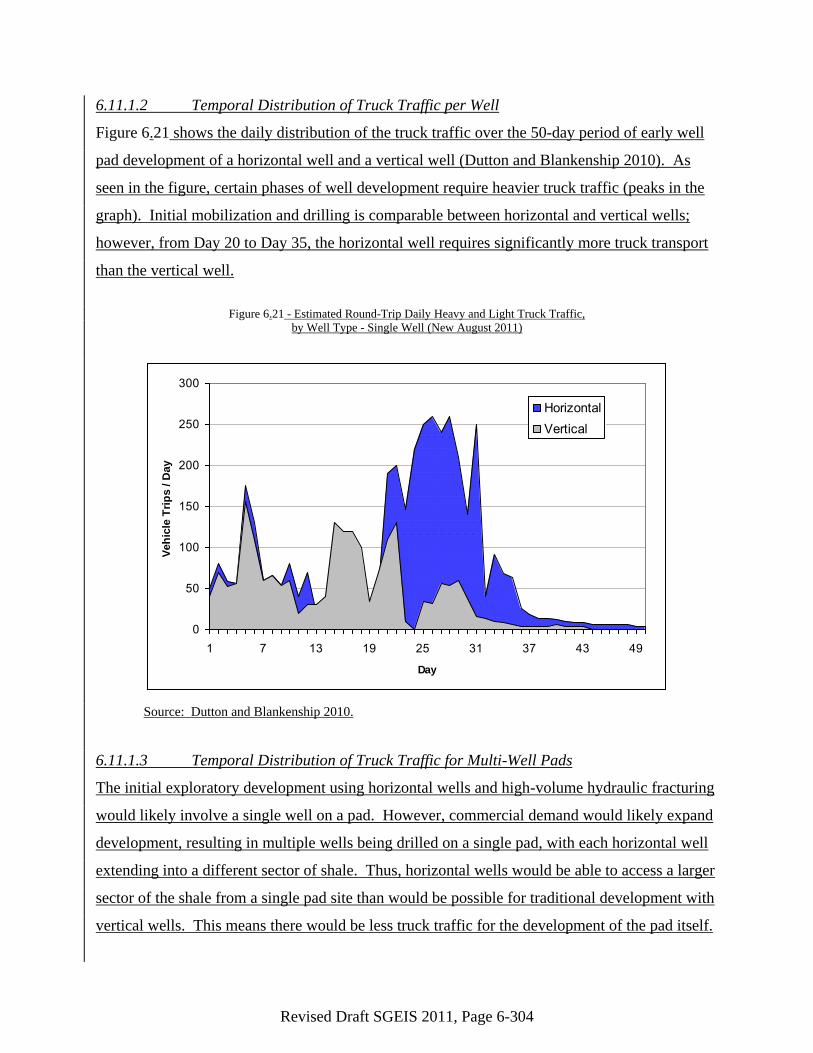
6.11.1.2 Temporal Distribution of Truck Traffic per Well
Figure 6.21 shows the daily distribution of the truck traffic over the 50-day period of early well
pad development of a horizontal well and a vertical well (Dutton and Blankenship 2010). As
seen in the figure, certain phases of well development require heavier truck traffic (peaks in the
graph). Initial mobilization and drilling is comparable between horizontal and vertical wells;
however, from Day 20 to Day 35, the horizontal well requires significantly more truck transport
than the vertical well.
Figure 6.21 - Estimated Round-Trip Daily Heavy and Light Truck Traffic,
by Well Type - Single Well (New August 2011)
0
50
100
150
200
250
300
1 7 13 19 25 31 37 43 49
Day
Veh
icle
Tri
ps / D
ay
Horizontal
Vertical
Source: Dutton and Blankenship 2010.
6.11.1.3 Temporal Distribution of Truck Traffic for Multi-Well Pads
The initial exploratory development using horizontal wells and high-volume hydraulic fracturing
would likely involve a single well on a pad. However, commercial demand would likely expand
development, resulting in multiple wells being drilled on a single pad, with each horizontal well
extending into a different sector of shale. Thus, horizontal wells would be able to access a larger
sector of the shale from a single pad site than would be possible for traditional development with
vertical wells. This means there would be less truck traffic for the development of the pad itself.
Revised Draft SGEIS 2011, Page 6-305
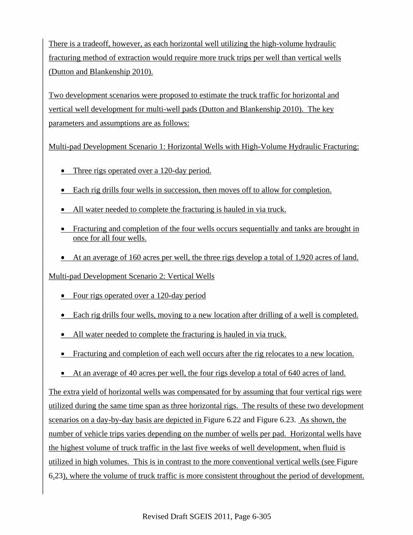
There is a tradeoff, however, as each horizontal well utilizing the high-volume hydraulic
fracturing method of extraction would require more truck trips per well than vertical wells
(Dutton and Blankenship 2010).
Two development scenarios were proposed to estimate the truck traffic for horizontal and
vertical well development for multi-well pads (Dutton and Blankenship 2010). The key
parameters and assumptions are as follows:
Multi-pad Development Scenario 1: Horizontal Wells with High-Volume Hydraulic Fracturing:
Three rigs operated over a 120-day period.
Each rig drills four wells in succession, then moves off to allow for completion.
All water needed to complete the fracturing is hauled in via truck.
Fracturing and completion of the four wells occurs sequentially and tanks are brought in
once for all four wells.
At an average of 160 acres per well, the three rigs develop a total of 1,920 acres of land.
Multi-pad Development Scenario 2: Vertical Wells
Four rigs operated over a 120-day period
Each rig drills four wells, moving to a new location after drilling of a well is completed.
All water needed to complete the fracturing is hauled in via truck.
Fracturing and completion of each well occurs after the rig relocates to a new location.
At an average of 40 acres per well, the four rigs develop a total of 640 acres of land.
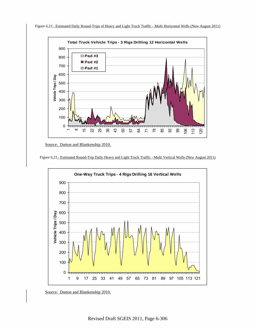
The extra yield of horizontal wells was compensated for by assuming that four vertical rigs were
utilized during the same time span as three horizontal rigs. The results of these two development
scenarios on a day-by-day basis are depicted in Figure 6.22 and Figure 6.23. As shown, the
number of vehicle trips varies depending on the number of wells per pad. Horizontal wells have
the highest volume of truck traffic in the last five weeks of well development, when fluid is
utilized in high volumes. This is in contrast to the more conventional vertical wells (see Figure
6.23), where the volume of truck traffic is more consistent throughout the period of development.
Revised Draft SGEIS 2011, Page 6-306
Figure 6.22 - Estimated Daily Round-Trips of Heavy and Light Truck Traffic - Multi Horizontal Wells (New August 2011)
Source: Dutton and Blankenship 2010.
Figure 6.23 - Estimated Round-Trip Daily Heavy and Light Truck Traffic - Multi Vertical Wells (New August 2011)
Source: Dutton and Blankenship 2010.
Total Truck Vehicle Trips - 3 Rigs Drilling 12 Horizontal Wells
0
100
200
300
400
500
600
700
800
900
1 8
15
22
29
36
43
50
57
64
71
78
85
92
99
106
113
120
Veh
icle
Tri
ps / D
ay
Pad #3
Pad #2
Pad #1
One-Way Truck Trips - 4 Rigs Drilling 16 Vertical Wells
0
100
200
300
400
500
600
700
800
900
1 9 17 25 33 41 49 57 65 73 81 89 97 105 113 121
Ve
hic
le T
rip
s / D
ay
Revised Draft SGEIS 2011, Page 6-307
The major conclusions to be drawn from this comparison of the truck traffic resulting from the
use of horizontal and vertical wells are as follows (Dutton and Blankenship 2010):
Peak-day traffic volumes given sequential completions with multiple rigs drilling
horizontal wells along the same access road could be substantially higher than those for
multiple rigs drilling vertical wells.
The larger the area drained per horizontal well and the drilling of multiple wells from a
pad without moving a rig offsets some of the increase in truck traffic associated with the
high-volume fracturing.
Based on industry data and other assumptions applied for these scenarios, the total
number of vehicle trips generated by the three rigs drilling 12 horizontal wells is roughly
equivalent to the number of vehicle trips associated with four rigs drilling 16 vertical
wells. However, the horizontal wells require three-times the amount of land (1,920 acres
for horizontal wells versus 640 acres for vertical wells). Thus, developing the same
amount of land using vertical wells would either require three times longer, or would
require deployment of 12 rigs during the same period, effectively tripling the total
number of trips and result in peak daily traffic volumes above the levels associated with
horizontal wells.
Based upon the information presented in these two development scenarios, utilizing horizontal
wells and high-volume hydraulic fracturing rather than vertical wells to access a section of land
would reduce the total amount of truck traffic. However, because vertical well hydraulic
fracturing is not as efficient in its extraction of natural gas, it is not always economically feasible
for operators to pursue. Currently, it is estimated that 10% of the wells drilled to develop low-
permeability reservoirs with high-volume hydraulic fracturing will be vertical. Thus, the number
of permits requested by applicants and issued by NYSDEC has not been fully reached.
Horizontal drilling with high-volume hydraulic fracturing would be expected to result in a
substantial increase in permits, well construction, and truck traffic over what is present in the
current environment.
6.11.2 Increased Traffic on Roadways
As described in Section 6.18, Socioeconomics, three possible development scenarios are being
assessed in this SGEIS to reflect the uncertainties associated with the future development of
natural gas reserves in the Marcellus and Utica Shales – a high, medium and low development
scenario. Each development scenario is defined by the number of vertical and horizontal wells
drilled annually. (A summary of the development scenarios is provided in Section 6.8). Based
on the number of wells estimated in each development scenario and the estimated number of
Revised Draft SGEIS 2011, Page 6-308
truck trips per well as discussed above in Section 6.1.1, the total estimated truck trips for all
wells developed annually is provided in Table 6.63. Annual trips are projected for Years 1
through 30 in 5-year increments. Estimated truck trips are provided for the three representative
regions (Regions A, B, and C), New York State outside of the three regions, and statewide.
The proposed action would also have an impact on traffic on federal, state, county, regional
local roadways. Given the generic nature of this analysis, and the lack of specific well pad
locations to permit the identification of specific road-segment impacts, the projected increase in
average annual daily traffic (AADT) and the associated impact on the level of service on specific
roadway segments, interchanges, and intersections cannot be determined. The AADT on
roadways can vary significantly, depending largely on functional class, and particularly whether
the count was taken in heavily populated communities or in proximity to heavily traveled
intersections/interchanges. Trucks traveling on higher level roadways along arterials and major
collectors are not anticipated to have a significant impact on traffic patterns and traffic flow, as
these roads are designed for a high level of vehicle traffic, and the anticipated increase in the
level of traffic associated with this action would only represent a small, incremental change in
existing conditions. However, certain local roads and minor collectors would likely experience
congestion during certain times of the day or during certain periods of well development.
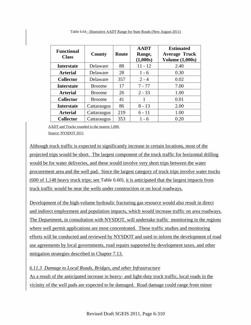
Table 6.64 illustrates this variation by providing the highest and lowest AADT on three
functional class roads in three counties, one in each of the representative regions. The counts
presented are the lowest and highest counts on the identified road in the designated functional
class in the county.
On some roads, truck traffic generated by high-volume hydraulic fracturing operations may be
small compared to total AADT, as would be the case on I-17 in Binghamton, where AADT was
approximately 77,000 vehicles. In other cases, and particularly on collectors and minor arterials,
traffic from high-volume hydraulic fracturing could be a large share of AADT. Truck traffic
from high-volume hydraulic fracturing operations could also be a large share of total daily truck
traffic on specific stretches of certain interstates and be much larger than existing truck volumes
on lower functional class roads that serve natural gas wells or link the wells to major truck heads
such as water supply, rail trans-loading, and staging areas.

Revised Draft SGEIS 2011, Page 6-309
Table 6.63 - Estimated Annual Heavy Truck Trips (in thousands) (New August 2011)
Region A Region B Region C
Counties Broome, Chemung, Tioga, Delaware, Otsego, Sullivan Cattaraugus, Chautauqua Rest of New York State State-Wide Totals
Low Development Scenario
Year Horizontal Vertical Total Horizontal Vertical Total Horizontal Vertical Total Horizontal Vertical Total Horizontal Vertical Total
1 4,334 226 4,561 2,053 113 2,166 456 0 456 1,597 113 1,710 8,441 453 8,893
5 21,216 1,245 22,460 9,809 566 10,375 2,053 113 2,166 9,353 453 9,806 42,431 2,376 44,807
10 42,431 2,376 44,807 19,391 1,132 20,522 4,334 226 4,561 18,478 1,018 19,496 84,634 4,752 89,387
15 42,431 2,376 44,807 19,391 1,132 20,522 4,334 226 4,561 18,478 1,018 19,496 84,634 4,752 89,387
20 42,431 2,376 44,807 19,391 1,132 20,522 4,334 226 4,561 18,478 1,018 19,496 84,634 4,752 89,387
25 42,431 2,376 44,807 19,391 1,132 20,522 4,334 226 4,561 18,478 1,018 19,496 84,634 4,752 89,387
30 42,431 2,376 44,807 19,391 1,132 20,522 4,334 226 4,561 18,478 1,018 19,496 84,634 4,752 89,387
Average Development Scenario
Year Horizontal Vertical Total Horizontal Vertical Total Horizontal Vertical Total Horizontal Vertical Total Horizontal Vertical Total
1 16,881 1,018 17,900 7,756 453 8,209 1,597 113 1,710 7,528 339 7,868 33,763 1,924 35,686
5 84,634 4,752 89,387 39,009 2,150 41,159 8,441 453 8,893 37,184 2,150 39,334 169,269 9,505 178,773
10 169,269 9,505 178,773 77,791 4,413 82,203 16,881 905 17,786 74,597 4,187 78,783 338,538 19,009 357,547
15 169,269 9,505 178,773 77,791 4,413 82,203 16,881 905 17,786 74,597 4,187 78,783 338,538 19,009 357,547
20 169,269 9,505 178,773 77,791 4,413 82,203 16,881 905 17,786 74,597 4,187 78,783 338,538 19,009 357,547
25 169,269 9,505 178,773 77,791 4,413 82,203 16,881 905 17,786 74,597 4,187 78,783 338,538 19,009 357,547
30 169,269 9,505 178,773 77,791 4,413 82,203 16,881 905 17,786 74,597 4,187 78,783 338,538 19,009 357,547
High Development Scenario
Year Horizontal Vertical Total Horizontal Vertical Total Horizontal Vertical Total Horizontal Vertical Total Horizontal Vertical Total
1 25,322 1,471 26,793 11,634 679 12,313 2,509 113 2,623 11,178 566 11,744 50,644 2,829 53,473
5 126,381 7,015 133,397 58,172 3,168 61,340 12,547 679 13,226 55,663 3,055 58,718 252,763 13,917 266,680
10 252,763 13,917 266,680 116,344 6,450 122,793 25,322 1,358 26,680 111,097 6,110 117,207 505,525 27,835 533,360
15 252,763 13,917 266,680 116,344 6,450 122,793 25,322 1,358 26,680 111,097 6,110 117,207 505,525 27,835 533,360
20 252,763 13,917 266,680 116,344 6,450 122,793 25,322 1,358 26,680 111,097 6,110 117,207 505,525 27,835 533,360
25 252,763 13,917 266,680 116,344 6,450 122,793 25,322 1,358 26,680 111,097 6,110 117,207 505,525 27,835 533,360
30 252,763 13,917 266,680 116,344 6,450 122,793 25,322 1,358 26,680 111,097 6,110 117,207 505,525 27,835 533,360
Revised Draft SGEIS 2011, Page 6-310
Table 6.64 - Illustrative AADT Range for State Roads (New August 2011)
Functional
Class County Route
AADT
Range,
(1,000s)
Estimated
Average Truck
Volume (1,000s)
Interstate Delaware 88 11 - 12 2.40
Arterial Delaware 28 1 - 6 0.30
Collector Delaware 357 2 - 4 0.02
Interstate Broome 17 7 - 77 7.00
Arterial Broome 26 2 - 33 1.00
Collector Broome 41 1 0.01
Interstate Cattaraugus 86 8 - 13 2.00
Arterial Cattaraugus 219 6 - 11 1.00
Collector Cattaraugus 353 1 - 6 0.20
AADT and Trucks rounded to the nearest 1,000.
Source: NYSDOT 2011
Although truck traffic is expected to significantly increase in certain locations, most of the
projected trips would be short. The largest component of the truck traffic for horizontal drilling
would be for water deliveries, and these would involve very short trips between the water
procurement area and the well pad. Since the largest category of truck trips involve water trucks
(600 of 1,148 heavy truck trips; see Table 6.60), it is anticipated that the largest impacts from
truck traffic would be near the wells under construction or on local roadways.
Development of the high-volume hydraulic fracturing gas resource would also result in direct
and indirect employment and population impacts, which would increase traffic on area roadways.
The Department, in consultation with NYSDOT, will undertake traffic monitoring in the regions
where well permit applications are most concentrated. These traffic studies and monitoring
efforts will be conducted and reviewed by NYSDOT and used to inform the development of road
use agreements by local governments, road repairs supported by development taxes, and other
mitigation strategies described in Chapter 7.13.
6.11.3 Damage to Local Roads, Bridges, and other Infrastructure
As a result of the anticipated increase in heavy- and light-duty truck traffic, local roads in the
vicinity of the well pads are expected to be damaged. Road damage could range from minor
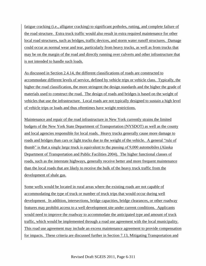
Revised Draft SGEIS 2011, Page 6-311
fatigue cracking (i.e., alligator cracking) to significant potholes, rutting, and complete failure of
the road structure. Extra truck traffic would also result in extra required maintenance for other
local road structures, such as bridges, traffic devices, and storm water runoff structures. Damage
could occur as normal wear and tear, particularly from heavy trucks, as well as from trucks that
may be on the margin of the road and directly running over culverts and other infrastructure that
is not intended to handle such loads.
As discussed in Section 2.4.14, the different classifications of roads are constructed to
accommodate different levels of service, defined by vehicle trips or vehicle class. Typically, the
higher the road classification, the more stringent the design standards and the higher the grade of
materials used to construct the road. The design of roads and bridges is based on the weight of
vehicles that use the infrastructure. Local roads are not typically designed to sustain a high level
of vehicle trips or loads and thus oftentimes have weight restrictions.
Maintenance and repair of the road infrastructure in New York currently strains the limited
budgets of the New York State Department of Transportation (NYSDOT) as well as the county
and local agencies responsible for local roads. Heavy trucks generally cause more damage to
roads and bridges than cars or light trucks due to the weight of the vehicle. A general ―rule of
thumb‖ is that a single large truck is equivalent to the passing of 9,000 automobiles (Alaska
Department of Transportation and Public Facilities 2004). The higher functional classes of
roads, such as the interstate highways, generally receive better and more frequent maintenance
than the local roads that are likely to receive the bulk of the heavy truck traffic from the
development of shale gas.
Some wells would be located in rural areas where the existing roads are not capable of
accommodating the type of truck or number of truck trips that would occur during well
development. In addition, intersections, bridge capacities, bridge clearances, or other roadway
features may prohibit access to a well development site under current conditions. Applicants
would need to improve the roadway to accommodate the anticipated type and amount of truck
traffic, which would be implemented through a road use agreement with the local municipality.
This road use agreement may include an excess maintenance agreement to provide compensation
for impacts. These criteria are discussed further in Section 7.13, Mitigating Transportation and
Revised Draft SGEIS 2011, Page 6-312
Road Use Impacts. Section 7.13 also discusses additional ways that compensatory mitigation
may be applied to pay for damages.
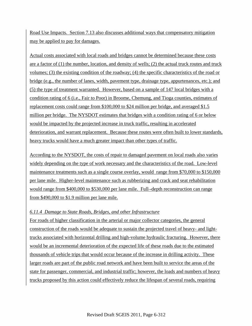
Actual costs associated with local roads and bridges cannot be determined because these costs
are a factor of (1) the number, location, and density of wells; (2) the actual truck routes and truck
volumes; (3) the existing condition of the roadway; (4) the specific characteristics of the road or
bridge (e.g., the number of lanes, width, pavement type, drainage type, appurtenances, etc.); and
(5) the type of treatment warranted. However, based on a sample of 147 local bridges with a
condition rating of 6 (i.e., Fair to Poor) in Broome, Chemung, and Tioga counties, estimates of
replacement costs could range from $100,000 to $24 million per bridge, and averaged $1.5
million per bridge. The NYSDOT estimates that bridges with a condition rating of 6 or below
would be impacted by the projected increase in truck traffic, resulting in accelerated
deterioration, and warrant replacement. Because these routes were often built to lower standards,
heavy trucks would have a much greater impact than other types of traffic.
According to the NYSDOT, the costs of repair to damaged pavement on local roads also varies
widely depending on the type of work necessary and the characteristics of the road. Low-level
maintenance treatments such as a single course overlay, would range from $70,000 to $150,000
per lane mile. Higher-level maintenance such as rubberizing and crack and seat rehabilitation
would range from $400,000 to $530,000 per lane mile. Full -depth reconstruction can range
from $490,000 to $1.9 million per lane mile.
6.11.4 Damage to State Roads, Bridges, and other Infrastructure
For roads of higher classification in the arterial or major collector categories, the general
construction of the roads would be adequate to sustain the projected travel of heavy- and light-
trucks associated with horizontal drilling and high-volume hydraulic fracturing. However, there
would be an incremental deterioration of the expected life of these roads due to the estimated
thousands of vehicle trips that would occur because of the increase in drilling activity. These
larger roads are part of the public road network and have been built to service the areas of the
state for passenger, commercial, and industrial traffic; however, the loads and numbers of heavy
trucks proposed by this action could effectively reduce the lifespan of several roads, requiring

Revised Draft SGEIS 2011, Page 6-313
unanticipated and early repairs or reconstruction, which would burden of the State and its
taxpayers.
When the cumulative and induced impacts of the total high-volume hydraulic fracturing gas
development are considered, the resulting traffic impacts can be considerable. The principal
cumulative traffic impacts would occur during drilling and well development. Impacts on the
road, bridge, and other infrastructure would be primarily from the cumulative impact of heavy
trucking.
Actual costs to roads of higher functional classification cannot be determined because these costs
are a factor of (1) the number, location and density of wells; (2) the actual truck routes and truck
volumes; (3) the existing condition of the roadway; (4) the specific characteristics of the road or
bridge (e.g., the number of lanes, width, pavement type, drainage type, appurtenances, etc.); and
(5) the type of treatment warranted, similar to the local roads discussed above.
However, based on a sample of 166 state bridges with a condition rating of 6 (i.e., Fair to Poor)
in Broome, Chemung, and Tioga counties, estimates of replacement costs could range from
$100,000 to $31 million per bridge, and averaged $3.3 million per bridge. The NYSDOT
estimates that bridges with a condition rating of 6 or below would be impacted by the projected
increase in truck traffic, resulting in accelerated deterioration, and warrant replacement.
According to the NYSDOT, the costs of repair to damaged pavement on state roads also varies
widely depending on the type of work necessary and the characteristics of the road. Low-level
maintenance treatments such as a single-course overlay, would range from $90,000 to $180,000
per lane mile. Higher-level maintenance such as rubberizing and crack and seat rehabilitation
would range from $540,000 to $790,000 per lane mile. Full depth reconstruction can range from
$910,000 to $2.1 million per lane mile.
Depending on the volume and location of high-volume hydraulic fracturing, there is a possibility
that a number of bridges and certain segments of state roads would require higher levels of
maintenance and possibly replacement. The extent of such road work that would be attributable
to high-volume hydraulic fracturing cannot be calculated because the proportion of truck and
vehicular traffic attributable to such operations compared to truck and vehicular traffic
Revised Draft SGEIS 2011, Page 6-314
attributable to other industries on any particular road would vary significantly. On collectors and
minor arterials, there is a potential for greater impacts from this activity because these routes
were often built to lower standards, and thus, heavy trucks would have a much greater impact
than other types of traffic. As a result, actual contribution of heavy trucks to road and bridge
deterioration would be greater than suggested by their proportion to total traffic. Conversely,
any additional traffic on higher functional class roads, and especially interstates and major
arterials, would result in little impact because these roads were built to higher construction and
pavement standards.
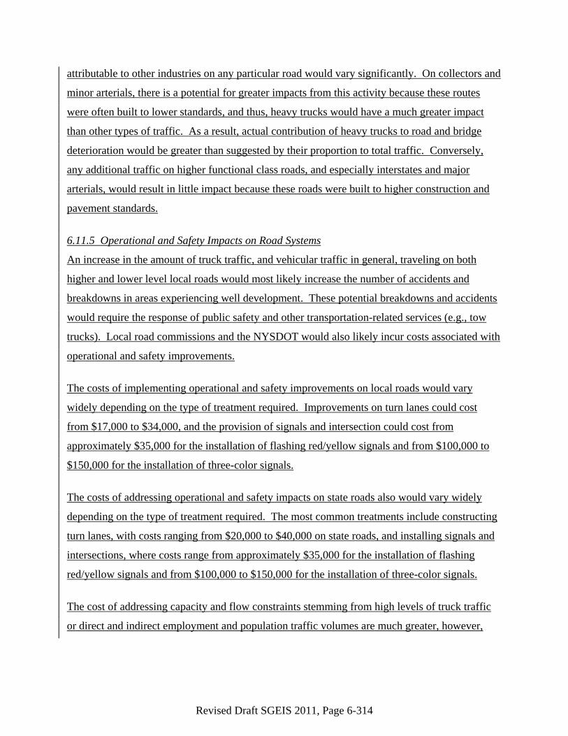
6.11.5 Operational and Safety Impacts on Road Systems
An increase in the amount of truck traffic, and vehicular traffic in general, traveling on both
higher and lower level local roads would most likely increase the number of accidents and
breakdowns in areas experiencing well development. These potential breakdowns and accidents
would require the response of public safety and other transportation-related services (e.g., tow
trucks). Local road commissions and the NYSDOT would also likely incur costs associated with
operational and safety improvements.
The costs of implementing operational and safety improvements on local roads would vary
widely depending on the type of treatment required. Improvements on turn lanes could cost
from $17,000 to $34,000, and the provision of signals and intersection could cost from
approximately $35,000 for the installation of flashing red/yellow signals and from $100,000 to
$150,000 for the installation of three-color signals.
The costs of addressing operational and safety impacts on state roads also would vary widely
depending on the type of treatment required. The most common treatments include constructing
turn lanes, with costs ranging from $20,000 to $40,000 on state roads, and installing signals and
intersections, where costs range from approximately $35,000 for the installation of flashing
red/yellow signals and from $100,000 to $150,000 for the installation of three-color signals.
The cost of addressing capacity and flow constraints stemming from high levels of truck traffic
or direct and indirect employment and population traffic volumes are much greater, however,
Revised Draft SGEIS 2011, Page 6-315
and might approach $1 million per lane per mile (roughly the cost of full reconstruction), not
including the costs of acquiring rights-of-way.
6.11.6 Transportation of Hazardous Materials
Vertical wells do not require the volumes of chemicals that would require consideration of
hazardous chemicals beyond the use of diesel fuel for the equipment on the surface. The truck
traffic supporting the development of the horizontal wells involving high-volume hydraulic
fracturing would be transporting a variety of equipment, supplies, and potentially hazardous
materials.
As described in Section 5.4 of the SGEIS, fracturing fluid is 98% freshwater and sand and 2% or
less chemical additives. There are 12 classes of chemical additives that could be in the
hazardous waste water being trucked to or from a location. Additive classes include: proppant,
acid, breaker, bactericide/biocide, clay stabilizer/control, corrosion inhibitor, cross linker,
friction reducer, gelling agent, iron control, scale inhibitor, and surfactant. These classes are
described in full detail in Section 5.4, Table 5.6. Although the composition of fracturing fluid
varies from one geologic basin or formation to another, the range of additive types available for
potential use remains the same. The selection may be driven by the formation and potential
interactions between additives, and not all additive types would be utilized in every fracturing
job (see Section 5.4). Table 5.7 (Section 5.4) shows the constituents of all hydraulic fracturing-
related chemicals submitted to NYSDEC to date for potential use at shale wells within New
York. Only a handful of these chemicals would be utilized at a single well. Data provided to
NYSDEC to date indicates that similar fracturing fluids are needed for vertical and horizontal
drilling methods.
Trucks transporting hazardous materials to the various well locations would be governed by
USDOT regulations, as discussed in Section 5.5 and Chapter 8. Transportation of any hazardous
materials always carries some risks from spills or accidents. Hazardous materials are moved
daily across the state without incident, but the additional transport resulting from horizontal
drilling poses an additional risk, which could be an adverse impact if spills occur.
Revised Draft SGEIS 2011, Page 6-316
6.11.7 Impacts on Rail and Air Travel
The development of high-volume hydraulic fracturing natural gas would require the movement
of large quantities of pipe, drilling equipment, and other large items from other locations and
from manufacturing sites that are likely far away from the well sites. Rail provides an
inexpensive and efficient means of moving such material. The final movement, from rail depots
to the well sites, would be accomplished with large trucks. The extent of rail and the choice of
unloading locations depends on the well sites and cannot be predicted at this time. However, the
use of rail to transport materials would have several predictable results:
Total truck traffic would decrease;
Truck traffic near the rail terminals would increase,
Truck traffic on the arterials between the terminals and well fields would increase.
These positive and negative impacts would likely alleviate some impacts but might exacerbate
impacts in neighborhoods along the routes to and from the rail centers. These impacts would
require examination as part of road use agreements.
The heavy, bulky, equipment utilized for horizontal drilling would not likely be transported by
air. However, the large numbers of temporary workers that the industry would employ would
likely utilize the network of small airports and commuter airlines that service New York State.
This would increase the traffic to and from these airports. None of the regional airports in New
York State are at capacity, so the air travel is not expected to be a significant impact. In fact, the
extra economic activity would be positive. However, residents that are along approach and
departure corridors would experience more noise from increased service by airplanes.
6.12 Community Character Impacts141
High-volume hydraulic fracturing operations could potentially have a significant impact on the
character of communities where drilling and production activities would occur. Both short-term
and long-term, impacts could result if this potentially large-scale industry were to start
operations. Experiences in Pennsylvania and West Virginia show that wholesale development of
141 Section 6.12, in its entirety, was provided by Ecology and Environment Engineering, P.C., August 2011, and was adapted by
the Department.

Revised Draft SGEIS 2011, Page 6-317
the low-permeable shale reserves could lead to changes in the economic, demographic, and
social characteristics of the affected communities.
While some of these impacts are expected to be significant, the determination of whether these
impacts are positive or negative cannot be made. Change would occur in the affected
communities, but how this change is viewed is subjective and would vary from individual to
individual. This section, therefore, seeks to identify expected changes that could occur to the
economic and social makeup of the impacted communities, but it does not attempt to make a
judgment on whether such change is beneficial or harmful to the local community character.
The amount of the change in community character that is expected to occur would be impacted
by several factors. However, the most important factors would be the speed at which high-
volume hydraulic fracturing activities would occur and the overall level of the natural gas
activities. Slow, moderate growth of the industry, if it were spread over several years, would
generate much less acute impacts than rapid expansion over a limited time. Community
character is constantly in a state of flux; a community‘s sense of place is constantly revised and
adapts as social, demographic, and economic conditions change. When these changes are
gradual, residents are given time to adapt and accommodate to the new conditions and typically
do not view them as negative. When these changes are abrupt and dramatic, residents typically
find them more adverse.
If the high-volume hydraulic fracturing operations reach some of the more optimistic
development levels described in previous sections, the size and structure of the regional
economies could be influenced by this new industry. Local communities that have experienced
declining employment and population levels for decades could quickly become some of the
fastest growing communities in the state. Traditional employment sectors could decline in
importance while new employment sectors, such as the natural gas extraction industry and its
suppliers, could expand in importance. Employment opportunities would increase in the
communities and the types of jobs offered would change.
Total population would increase in the communities and the demographic makeup of these
populations would change. In-migration resulting from the high-volume hydraulic fracturing

Revised Draft SGEIS 2011, Page 6-318
operations would bring a racially and ethnically diverse workforce into the area. Most of the
new population would be working age or their dependents. In addition, most of the employment
opportunities created would be for skilled blue collar jobs.
In addition to employment and demographic impacts, the proposed high-volume hydraulic
fracturing would greatly increase income and earnings throughout affected communities.
Royalty payments to local landowners, increased payroll earnings from the natural gas industry,
added profits to firms that supply the natural gas industry, and added earnings from all of the
induced economic activity that would occur in the communities would all add to the affluence of
the region. While total income in the communities would increase, this added income and
wealth would not be evenly distributed. Landowners that lease out their subsurface mineral
rights would benefit financially from the high-volume hydraulic fracturing operations; however,
those residents that do not own the subsurface mineral rights or chose not to exploit these rights
would not see the same financial benefits. Some entrepreneurs and property owners would see
large financial gains from the increase in economic activity, other residents may experience a
rise in living expenses without enjoying any corresponding financial gains.
In some areas, the housing market would experience an increase in value and price if there is not
sufficient outstanding supply to meet the increased demand. Existing property owners would
most likely benefit; residents not already property owners could experience price rises and
difficulties entering the market. Additional housing would most likely be constructed in response
to increased demand, and in certain instances such development could occur on currently
undeveloped land. Activities that achieve lower financial returns on property, such as
agriculture, may be considered less desirable compared to housing developments. While at the
same time, farmers who own large tracts of land could also benefit greatly from the royalty
payments on the new natural gas wells.
Local governments would see a rapid expansion in the amount of sales tax and property tax
generated by gas drilling and would now have the funding to complete a wide range of
community projects. At the same time, the large influx of population would demand additional
community services and facilities. Existing facilities would likely become overcrowded, and
additional new facilities would have to be built to accommodate this new population.
Revised Draft SGEIS 2011, Page 6-319
Commuting patterns in the affected communities would also change. An increase in traffic both
from the added truck transportation and from the additional population would likely increase
traffic on certain areas roadways and, as further explained in the Transportation subchapter,
would likely lead to the need for road improvements, reconstruction and repairs.
Ambient noise levels in the communities would likely increase as a direct result of drilling and
additional traffic at the well pads, and as a result of increased development in the region (see
Section 2.4.13). Aesthetic resources and viewsheds could be at least temporarily impacted and
changed during well pad construction and development (see Section 2.4.12).
6.13 Seismicity142
Economic development of natural gas from low permeability formations requires the target
formation to be hydraulically fractured to increase the rock permeability and expose more rock
surface to release the gas trapped within the rock. The hydraulic fracturing process fractures the
rock by controlled application of hydraulic pressure in the wellbore. The direction and length of
the fractures are managed by carefully controlling the applied pressure during the hydraulic
fracturing process.
The release of energy during hydraulic fracturing produces seismic pressure waves in the
subsurface. Microseismic monitoring commonly is performed to evaluate the progress of
hydraulic fracturing and adjust the process, if necessary, to limit the direction and length of the
induced fractures. Chapter 4 of this SGEIS presents background seismic information for New
York. Concerns associated with the seismic events produced during hydraulic fracturing are
discussed below.
6.13.1 Hydraulic Fracturing-Induced Seismicity
Seismic events that occur as a result of injecting fluids into the ground are termed ―induced.‖
There are two types of induced seismic events that may be triggered as a result of hydraulic
fracturing. The first is energy released by the physical process of fracturing the rock which
creates microseismic events that are detectable only with very sensitive monitoring equipment.
142 Alpha, 2009, Section 7; discussion was provided for NYSERDA by Alpha Environmental, Inc., and Alpha‘s references are
included for informational purposes.
Revised Draft SGEIS 2011, Page 6-320
Information collected during the microseismic events is used to evaluate the extent of fracturing
and to guide the hydraulic fracturing process. This type of microseismic event is a normal part
of the hydraulic fracturing process used in the development of both horizontal and vertical oil
and gas wells, and by the water well industry.
The second type of induced seismicity is fluid injection of any kind, including hydraulic
fracturing, which can trigger seismic events ranging from imperceptible microseismic, to small-
scale, ―felt‖ events, if the injected fluid reaches an existing geologic fault. A ―felt‖ seismic event
is when earth movement associated with the event is discernable by humans at the ground
surface. Hydraulic fracturing produces microseismic events, but different injection processes,
such as waste disposal injection or long term injection for enhanced geothermal, may induce
events that can be felt, as discussed in the following section. Induced seismic events can be
reduced by engineering design and by avoiding existing fault zones.
6.13.1.1 Background
Hydraulic fracturing consists of injecting fluid into a wellbore at a pressure sufficient to fracture
the rock within a designed distance from the wellbore. Other processes where fluid is injected
into the ground include deep well fluid disposal, fracturing for enhanced geothermal wells,
solution mining and hydraulic fracturing to improve the yield of a water supply well. The
similar aspect of these methods is that fluid is injected into the ground to fracture the rock;
however, each method also has distinct and important differences.
There are ongoing and past studies that have investigated small, felt, seismic events that may
have been induced by injection of fluids in deep disposal wells. These small seismic events are
not the same as the microseismic events triggered by hydraulic fracturing that can only be
detected with the most sensitive monitoring equipment. The processes that induce seismicity in
both cases are very different.
Deep well injection is a disposal technology which involves liquid waste being pumped under
moderate to high pressure, several thousand feet into the subsurface, into highly saline,
permeable injection zones that are confined by more shallow, impermeable strata (FRTR, August
Revised Draft SGEIS 2011, Page 6-321
12, 2009). The goal of deep well injection is to store the liquids in the confined formation(s)
permanently.
Carbon sequestration is also a type of deep well injection, but the carbon dioxide emissions from
a large source are compressed to a near liquid state. Both carbon sequestration and liquid waste
injection can induce seismic activity. Induced seismic events caused by deep well fluid injection
are typically less than a magnitude 3.0 and are too small to be felt or to cause damage. Rarely,
fluid injection induces seismic events with moderate magnitudes, between 3.5 and 5.5, that can
be felt and may cause damage. Most of these events have been investigated in detail and have
been shown to be connected to circumstances that can be avoided through proper site selection
(avoiding fault zones) and injection design (Foxall and Friedmann, 2008).
Hydraulic fracturing also has been used in association with enhanced geothermal wells to
increase the permeability of the host rock. Enhanced geothermal wells are drilled to depths of
many thousands of feet where water is injected and heated naturally by the earth. The rock at the
target depth is fractured to allow a greater volume of water to be re-circulated and heated.
Recent geothermal drilling for commercial energy-producing geothermal projects have focused
on hot, dry, rocks as the source of geothermal energy (Duffield, 2003). The geologic conditions
and rock types for these geothermal projects are in contrast to the shallower sedimentary rocks
targeted for natural gas development. The methods used to fracture the igneous rock for
geothermal projects involve high pressure applied over a period of many days or weeks
(Florentin 2007 and Geoscience Australia, 2009). These methods differ substantially from the
lower pressures and short durations used for natural gas well hydraulic fracturing.
Hydraulic fracturing is a different process that involves injecting fluid under higher pressure for
shorter periods than the pressure level maintained in a fluid disposal well. A horizontal well is
fractured in stages so that the pressure is repeatedly increased and released over a short period of
time necessary to fracture the rock. The subsurface pressures for hydraulic fracturing are
sustained typically for one or two days to stimulate a single well, or for approximately two
weeks at a multi-well pad. The seismic activity induced by hydraulic fracturing is only
detectable at the surface by very sensitive equipment.
Revised Draft SGEIS 2011, Page 6-322
Avoiding pre-existing fault zones minimizes the possibility of triggering movement along a fault
through hydraulic fracturing. It is important to avoid injecting fluids into known, significant,
mapped faults when hydraulic fracturing. Generally, operators would avoid faults because they
disrupt the pressure and stress field and the hydraulic fracturing process. The presence of faults
also potentially reduces the optimal recovery of gas and the economic viability of a well or wells.
Injecting fluid into the subsurface can trigger shear slip on bedding planes or natural fractures
resulting in microseismic events. Fluid injection can temporarily increase the stress and pore
pressure within a geologic formation. Tensile stresses are formed at each fracture tip, creating
shear stress (Pinnacle; ―FracSeis;‖ August 11, 2009). The increases in pressure and stress reduce
the normal effective stress acting on existing fault, bedding, or fracture planes. Shear stress then
overcomes frictional resistance along the planes, causing the slippage (Bou-Rabee and Nur,
2002). The way in which these microseismic events are generated is different than the way in
which microseisms occur from the energy release when rock is fractured during hydraulic
fracturing.
The amount of displacement along a plane that is caused by hydraulic fracturing determines the
resultant microseism‘s amplitude. The energy of one of these events is several orders of
magnitude less than that of the smallest earthquake that a human can feel (Pinnacle;
―Microseismic;‖ August 11, 2009). The smallest measurable seismic events are typically
between 1.0 and 2.0 magnitude. In contrast, seismic events with magnitude 3.0 are typically
large enough to be felt by people. Many induced microseisms have a negative value on the
MMS. Pinnacle Technologies, Inc. has determined that the characteristic frequencies of
microseisms are between 200 and 2,000 Hertz; these are high-frequency events relative to typical
seismic data. These small magnitude events are monitored using extremely sensitive instruments
that are positioned at the fracture depth in an offset wellbore or in the treatment well (Pinnacle;
―Microseismic;‖ August 11, 2009). The microseisms from hydraulic fracturing can barely be
measured at ground surface by the most sensitive instruments (Sharma, personal communication,
August 7, 2009).
There are no seismic monitoring protocols or criteria established by regulatory agencies that are
specific to high volume hydraulic fracturing. Nonetheless, operators monitor the hydraulic
Revised Draft SGEIS 2011, Page 6-323
fracturing process to optimize the results for successful gas recovery. It is in the operator‘s best
interest to closely control the hydraulic fracturing process to ensure that fractures are propagated
in the desired direction and distance and to minimize the materials and costs associated with the
process.
The routine microseismic monitoring that is performed during hydraulic fracturing serves to
evaluate, guide, and control the process and is important in optimizing well treatments. Multiple
receivers on a wireline array are placed in one or more offset borings (new, unperforated well(s)
or older well(s) with production isolated) or in the treatment well to detect microseisms and to
monitor the hydraulic fracturing process. The microseism locations are triangulated using the
arrival times of the various p- and s-waves with the receivers in several wells, and using the
formation velocities to determine the location of the microseisms. A multi-level vertical array of
receivers is used if only one offset observation well is available. The induced fracture is
interpreted to lie within the envelope of mapped microseisms (Pinnacle; ―FracSeis;‖ August 11,
2009).
Data requirements for seismic monitoring of a hydraulic fracturing treatment include formation
velocities (from a dipole sonic log or cross-well tomogram), well surface and deviation surveys,
and a source shot in the treatment well to check receiver orientations, formation velocities and
test capabilities. Receiver spacing is selected so that the total aperture of the array is about half
the distance between the two wells. At least one receiver should be in the treatment zone, with
another located above and one below this zone. Maximum observation distances for
microseisms should be within approximately 2,500 feet of the treatment well; the distance is
dependent upon formation properties and background noise level (Pinnacle; ―FracSeis;‖ August
11, 2009).
6.13.1.2 Recent Investigations and Studies
Hydraulic fracturing has been used by oil and gas companies to stimulate production of vertical
wells in New York State since the 1950s. Despite this long history, there are no records of
induced seismicity caused by hydraulic fracturing in New York State. The only induced
seismicity studies that have taken place in New York State are related to seismicity suspected to
have been caused by waste fluid disposal by injection and a mine collapse, as identified in
Revised Draft SGEIS 2011, Page 6-324
Section 4.5.4. The seismic events induced at the Dale Brine Field (Section 4.5.4) were the result
of the injection of fluids for extended periods of time at high pressure for the purpose of salt
solution mining. This process is significantly different from the hydraulic fracturing process that
would be undertaken for developing the Marcellus and other low-permeability shales in New
York.
Gas producers in Texas have been using horizontal drilling and high-volume hydraulic fracturing
to stimulate gas production in the Barnett Shale for the last decade. The Barnett is geologically
similar to the Marcellus, but is found at a greater depth; it is a deep shale with gas stored in
unconnected pore spaces and adsorbed to the shale matrix. High-volume hydraulic fracturing
allows recovery of the gas from the Barnett to be economically feasible. The horizontal drilling
and high-volume hydraulic fracturing methods used for the Barnett Shale play are similar to
those that would be used in New York State to develop the Marcellus, Utica, and other gas
bearing shales.
Alpha contacted several researchers and geologists who are knowledgeable about seismic
activity in New York and Texas, including:
Mr. John Armbruster, Staff Associate, Lamont-Doherty Earth Observatory, Columbia
University;
Dr. Cliff Frohlich, Associate Director of the Texas Institute for Geophysics, The
University of Texas at Austin;
Dr. Won-Young Kim, Doherty Senior Research Scientist, Lamont-Doherty Earth
Observatory, Columbia University;
Mr. Eric Potter, Associate Director of the Texas Bureau of Economic Geology, The
University of Texas at Austin;
Mr. Leonardo Seeber, Doherty Senior Research Scientist, Lamont-Doherty Earth
Observatory, Columbia University;
Dr. Mukul Sharma, Professor of Petroleum and Geosystems Engineering, The University
of Texas at Austin; and
Dr. Brian Stump, Albritton Professor, Southern Methodist University.
Revised Draft SGEIS 2011, Page 6-325
None of these researchers have knowledge of any seismic events that could be explicitly related
to hydraulic fracturing in a shale gas well. Mr. Eric Potter stated that approximately 12,500
wells in the Barnett play and several thousand wells in the East Texas Basin (which target tight
gas sands) have been stimulated using hydraulic fracturing in the last decade, and there have
been no documented connections between wells being fractured hydraulically and felt quakes
(personal communication, August 9, 2009). Dr. Mukul Sharma confirmed that microseismic
events associated with hydraulic fracturing can only be detected using very sensitive instruments
(personal communication, August 7, 2009).
The Bureau of Geology, the University of Texas‘ Institute of Geophysics, and Southern
Methodist University (SMU) are planning to study earthquakes measured in the vicinity of the
Dallas - Fort Worth (DFW) area, and Cleburne, Texas, that appear to be associated with salt
water disposal wells, and oil and gas wells. The largest quakes in both areas were magnitudes of
3.3, and more than 100 earthquakes with magnitudes greater than 1.5 have been recorded in the
DFW area in 2008 and 2009. There is considerable oil and gas drilling and deep brine disposal
wells in the area and a small fault extends beneath the DFW area. Dr. Frohlich recently stated
that ―[i]t‘s always hard to attribute a cause to an earthquake with absolute certainty.‖ Dr.
Frohlich has two manuscripts in preparation with SMU describing the analysis of the DFW
activity and the relationship with gas production activities (personal communication, August 4
and 10, 2009). Neither of these manuscripts was available before this document was completed.
Nonetheless, information posted online by SMU (2009) states that the research suggests that the
earthquakes seem to have been caused by injections associated with a deep production brine
disposal well, and not with hydraulic fracturing operations.
6.13.1.3 Correlations between New York and Texas
The gas plays of interest, the Marcellus and Utica Shales in New York and the Barnett Shale in
Texas, are relatively deep, low-permeability, gas shales deposited during the Paleozoic Era.
Horizontal drilling and high-volume hydraulic fracturing methods are required for successful,
economical gas production. The Marcellus Shale was deposited during the early Devonian, and
the slightly younger Barnett was deposited during the late Mississippian. The depth of the
Marcellus in New York ranges from exposure at the ground surface in some locations in the
northern Finger Lakes area to 7,000 feet or more below the ground surface at the Pennsylvania
Revised Draft SGEIS 2011, Page 6-326
border in the Delaware River valley. The depth of the Utica Shale in New York ranges from
exposure at the ground surface along the southern Adirondacks to more than 10,000 feet along
the New York Pennsylvania border.
Conditions for economic gas recovery likely are present only in portions of the Marcellus and
Utica members, as described in Chapter 4. The thickness of the Marcellus and Utica in New
York ranges from less than 50 feet in the southwestern portion of the state to approximately 250
feet at the south-central border. The Barnett Shale is 5,000 to 8,000 feet below the ground
surface and 100 to 500 feet thick (Halliburton; August 12, 2009). It has been estimated that the
entire Marcellus Shale may hold between 168 and 516 trillion cubic feet of gas; in contrast, the
Barnett has in-place gas reserves of approximately 26.2 trillion cubic feet (USGS, 2009A) and
covers approximately 4 million acres.
The only known induced seismicity associated with the stimulation of the Barnett wells are
microseisms that are monitored with downhole transducers. These small-magnitude events
triggered by the fluid pressure provide data to the operators to monitor and improve the
fracturing operation and maximize gas production. The hydraulic fracturing and monitoring
operations in the Barnett have provided operators with considerable experience with conditions
similar to those that would be encountered in New York State. Based on the similarity of
conditions, similar results are anticipated for New York State; that is, the microseismic events
would be unfelt at the surface and no damage would result from the induced microseisms.
Operators are likely to monitor the seismic activity in New York, as in Texas, to optimize the
hydraulic fracturing methods and results.
6.13.1.4 Affects of Seismicity on Wellbore Integrity
Wells are designed to withstand deformation from seismic activity. The steel casings used in
modern wells are flexible and are designed to deform to prevent rupture. The casings can
withstand distortions much larger than those caused by earthquakes, except for those very close
to an earthquake epicenter. The magnitude 6.8 earthquake event in 1983 that occurred in
Coalinga, California, damaged only 14 of the 1,725 nearby active oilfield wells, and the energy
released by this event was thousands of times greater than the microseismic events resulting from
hydraulic fracturing. Earthquake-damaged wells can often be re-completed. Wells that cannot
Revised Draft SGEIS 2011, Page 6-327
be repaired are plugged and abandoned (Foxall and Friedmann, 2008). Induced seismicity from
hydraulic fracturing is of such small magnitude that it is not expected to have any effect on
wellbore integrity.
6.13.2 Summary of Potential Seismicity Impacts
The issues associated with seismicity related to hydraulic fracturing addressed herein include
seismic events generated from the physical fracturing of the rock, and possible seismic events
produced when fluids are injected into existing faults.
The possibility of fluids injected during hydraulic fracturing the Marcellus or Utica Shales
reaching a nearby fault and triggering a seismic event are remote for several reasons. The
locations of major faults in New York have been mapped (Figure 4.13) and few major or
seismically active faults exist within the fairways for the Marcellus and Utica Shales. Similarly,
the paucity of historic seismic events and the low seismic risk level in the fairways for these
shales indicates that geologic conditions generally are stable in these areas. By definition, faults
are planes or zones of broken or fractured rock in the subsurface. The geologic conditions
associated with a fault generally are unfavorable for hydraulic fracturing and economical
production of natural gas. As a result, operators typically endeavor to avoid faults for both
practical and economic considerations. It is prudent for an applicant for a drilling permit to
evaluate and identify known, significant, mapped, faults within the area of effect of hydraulic
fracturing and to present such information in the drilling permit application. It is Alpha‘s
opinion that an independent pre-drilling seismic survey probably is unnecessary in most cases
because of the relatively low level of seismic risk in the fairways of the Marcellus and Utica
Shales. Additional evaluation or monitoring may be necessary if hydraulic fracturing fluids
might reach a known, significant, mapped fault, such as the Clarendon-Linden fault system.
Recent research has been performed to investigate induced seismicity in an area of active
hydraulic fracturing for natural gas development near Fort Worth, Texas. Studies also were
performed to evaluate the cause of the earthquakes associated with the solution mining activity
near the Clarendon-Linden fault system near Dale, NY in 1971. The studies indicated that the
likely cause of the earthquakes was the injection of fluid for production brine disposal for the
incidents in Texas, and the injection of fluid for solution mining for the incidents in Dale, NY

Revised Draft SGEIS 2011, Page 6-328
The studies in Texas also indicate that hydraulic fracturing is not likely the source of the
earthquakes.
The hydraulic fracturing methods used for enhanced geothermal energy projects are appreciably
different than those used for natural gas hydraulic fracturing. Induced seismicity associated with
geothermal energy projects occurs because the hydraulic fracturing is performed at greater
depths, within different geologic conditions, at higher pressures, and for substantially longer
durations compared with the methods used for natural gas hydraulic fracturing.
There is a reasonable base of knowledge and experience related to seismicity induced by
hydraulic fracturing. Information reviewed in preparing this discussion indicates that there is
essentially no increased risk to the public, infrastructure, or natural resources from induced
seismicity related to hydraulic fracturing. The microseisms created by hydraulic fracturing are
too small to be felt, or to cause damage at the ground surface or to nearby wells.
Seismic monitoring by the operators is performed to evaluate, adjust, and optimize the hydraulic
fracturing process. Monitoring beyond that which is typical for hydraulic fracturing does not
appear to be warranted, based on the negligible risk posed by the process and very low seismic
magnitude. The existing and well-established seismic monitoring network in New York is
sufficient to document the locations of larger-scale seismic events and would continue to provide
additional data to monitor and evaluate the likely sources of seismic events that are felt.
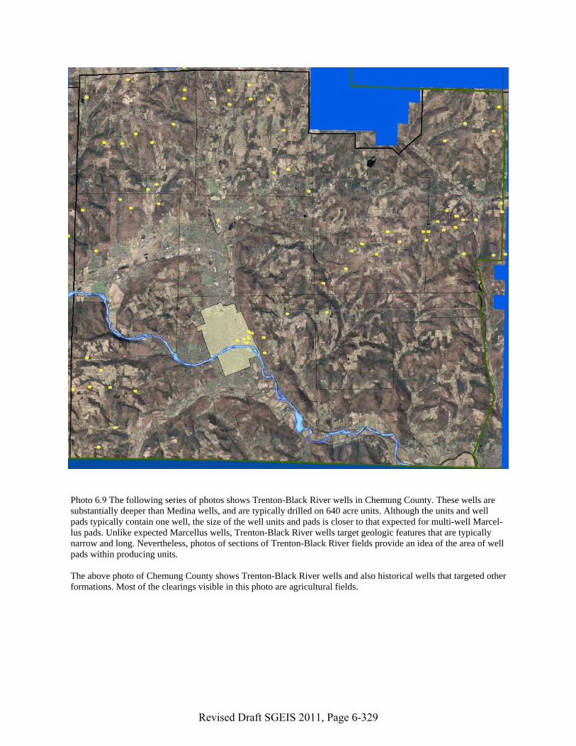
Photo 6.9 The following series of photos shows Trenton-Black River wells in Chemung County. These wells are substantially deeper than Medina wells, and are typically drilled on 640 acre units. Although the units and well pads typically contain one well, the size of the well units and pads is closer to that expected for multi-well Marcel-lus pads. Unlike expected Marcellus wells, Trenton-Black River wells target geologic features that are typically narrow and long. Nevertheless, photos of sections of Trenton-Black River fields provide an idea of the area of well pads within producing units. The above photo of Chemung County shows Trenton-Black River wells and also historical wells that targeted other formations. Most of the clearings visible in this photo are agricultural fields.
Revised Draft SGEIS 2011, Page 6-329
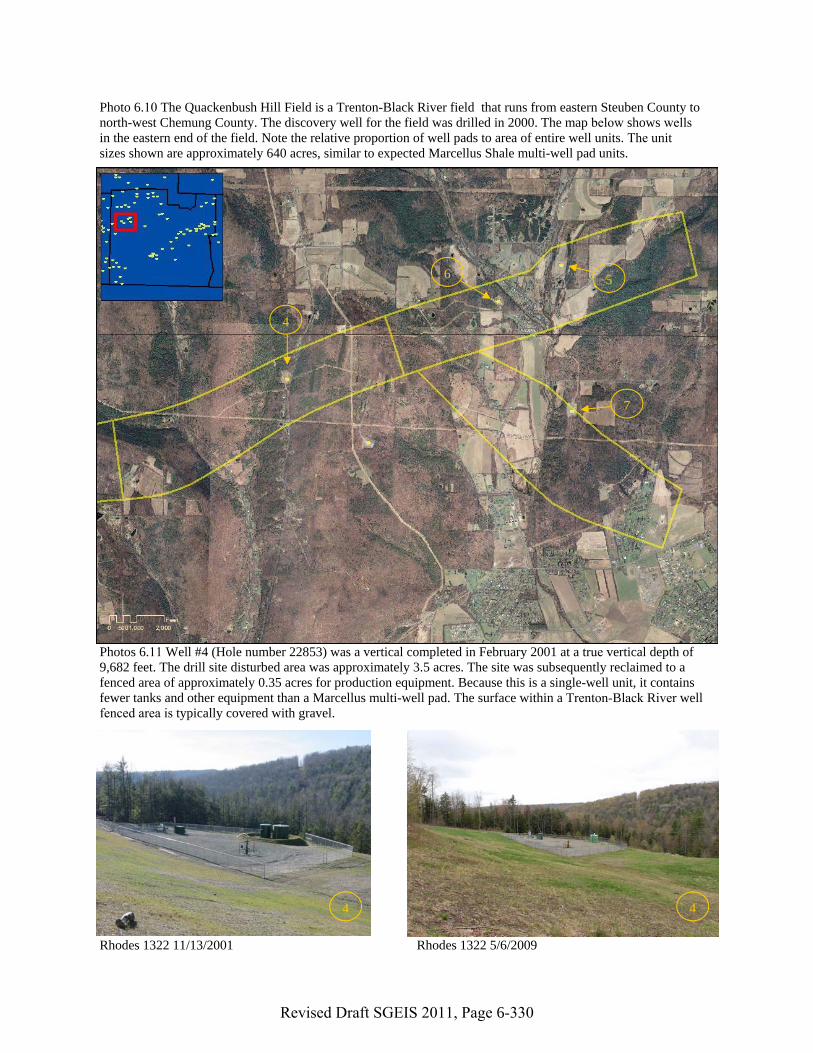
Photo 6.10 The Quackenbush Hill Field is a Trenton-Black River field that runs from eastern Steuben County to north-west Chemung County. The discovery well for the field was drilled in 2000. The map below shows wells in the eastern end of the field. Note the relative proportion of well pads to area of entire well units. The unit sizes shown are approximately 640 acres, similar to expected Marcellus Shale multi-well pad units.
5
4
Photos 6.11 Well #4 (Hole number 22853) was a vertical completed in February 2001 at a true vertical depth of 9,682 feet. The drill site disturbed area was approximately 3.5 acres. The site was subsequently reclaimed to a fenced area of approximately 0.35 acres for production equipment. Because this is a single-well unit, it contains fewer tanks and other equipment than a Marcellus multi-well pad. The surface within a Trenton-Black River well fenced area is typically covered with gravel.
Rhodes 1322 11/13/2001 Rhodes 1322 5/6/2009
4 4
6
7
Revised Draft SGEIS 2011, Page 6-330
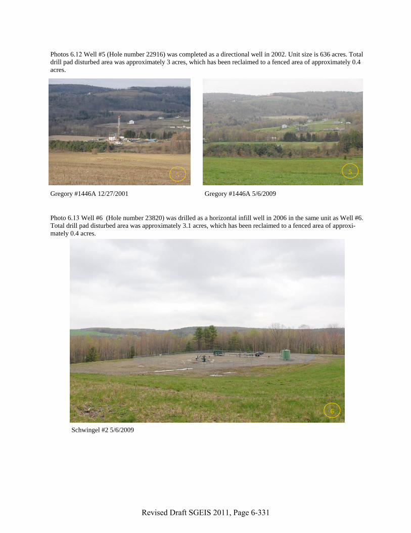
Schwingel #2 5/6/2009
6
Photos 6.12 Well #5 (Hole number 22916) was completed as a directional well in 2002. Unit size is 636 acres. Total drill pad disturbed area was approximately 3 acres, which has been reclaimed to a fenced area of approximately 0.4 acres.
Gregory #1446A 12/27/2001 Gregory #1446A 5/6/2009
5 5
Photo 6.13 Well #6 (Hole number 23820) was drilled as a horizontal infill well in 2006 in the same unit as Well #6. Total drill pad disturbed area was approximately 3.1 acres, which has been reclaimed to a fenced area of approxi-mately 0.4 acres.
Revised Draft SGEIS 2011, Page 6-331
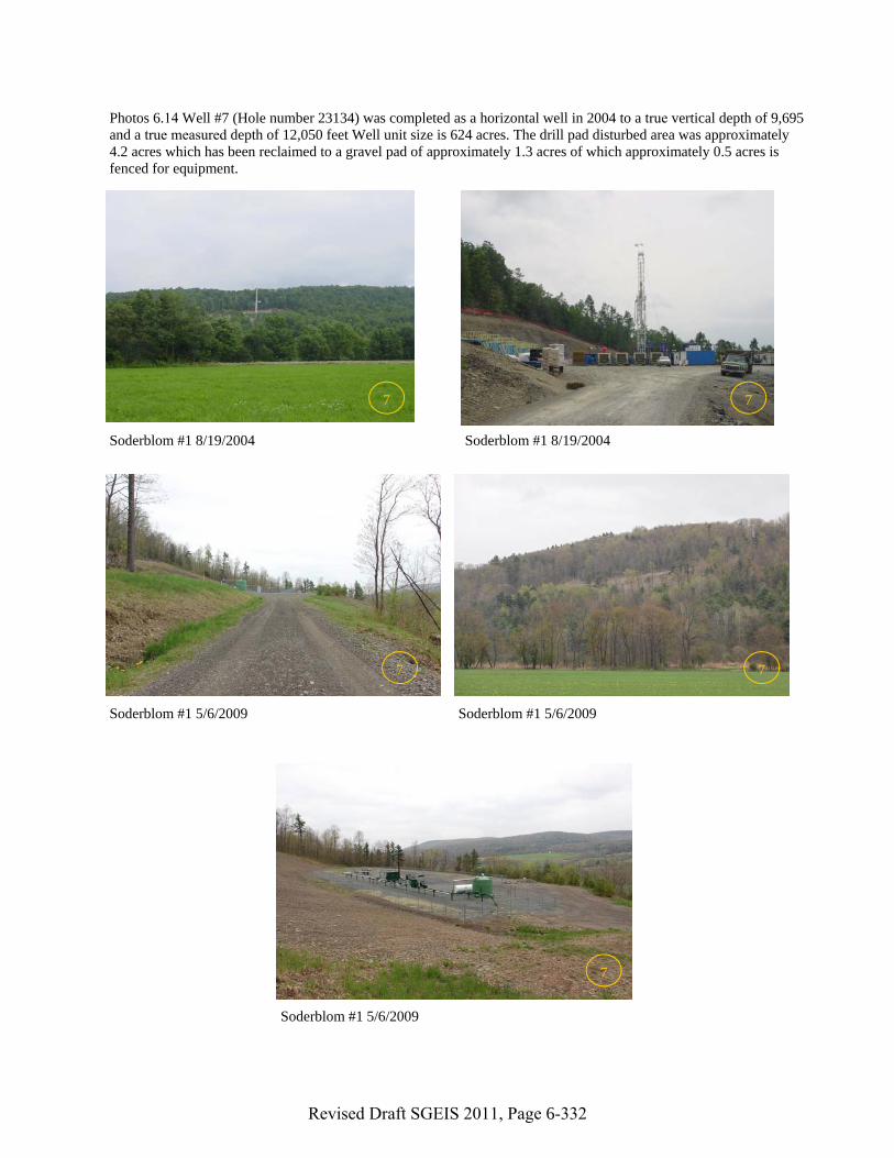
Soderblom #1 8/19/2004 Soderblom #1 8/19/2004
Soderblom #1 5/6/2009 Soderblom #1 5/6/2009
Photos 6.14 Well #7 (Hole number 23134) was completed as a horizontal well in 2004 to a true vertical depth of 9,695 and a true measured depth of 12,050 feet Well unit size is 624 acres. The drill pad disturbed area was approximately 4.2 acres which has been reclaimed to a gravel pad of approximately 1.3 acres of which approximately 0.5 acres is fenced for equipment.
Soderblom #1 5/6/2009
7 7
7 7
7
Revised Draft SGEIS 2011, Page 6-332
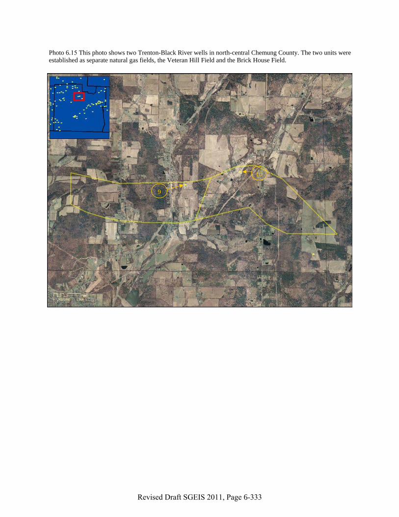
9
10
Photo 6.15 This photo shows two Trenton-Black River wells in north-central Chemung County. The two units were established as separate natural gas fields, the Veteran Hill Field and the Brick House Field.
Revised Draft SGEIS 2011, Page 6-333
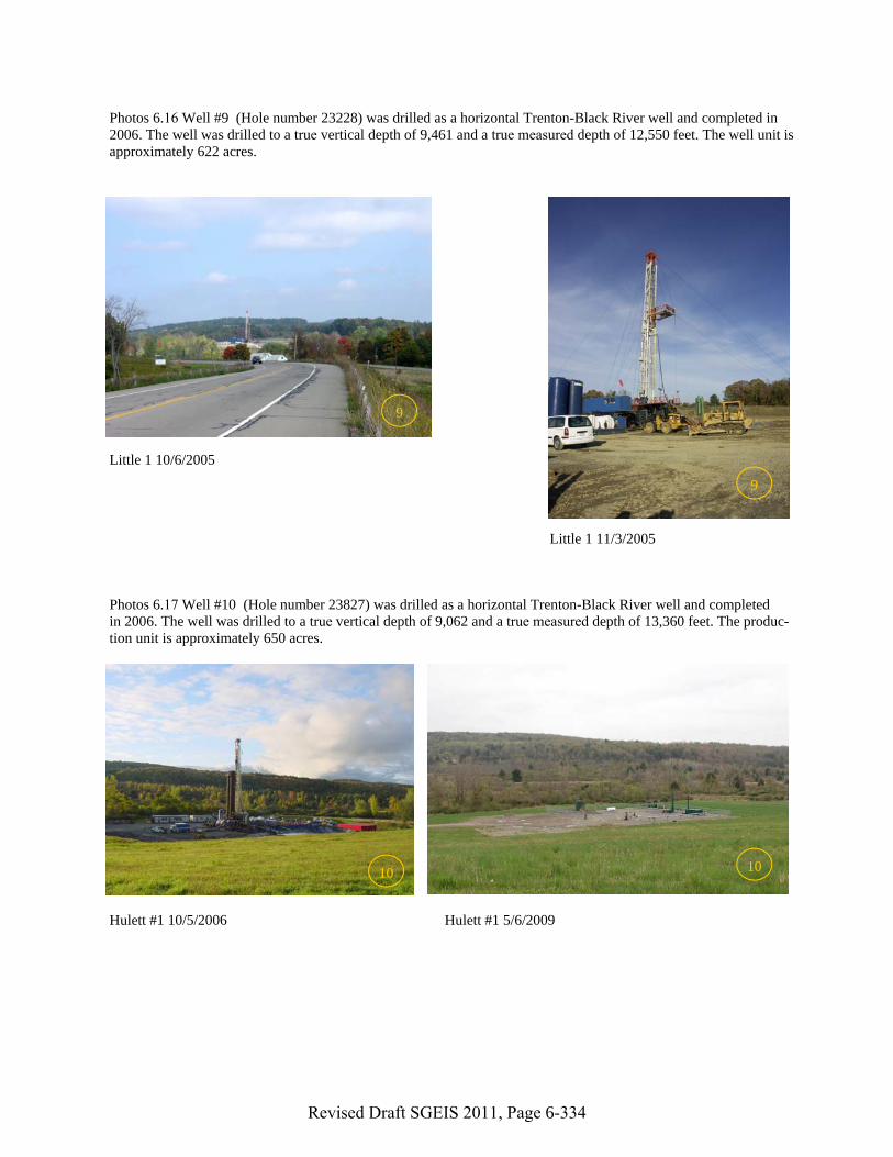
Hulett #1 10/5/2006 Hulett #1 5/6/2009
Little 1 10/6/2005
Little 1 11/3/2005
9
10
Photos 6.16 Well #9 (Hole number 23228) was drilled as a horizontal Trenton-Black River well and completed in 2006. The well was drilled to a true vertical depth of 9,461 and a true measured depth of 12,550 feet. The well unit is approximately 622 acres.
Photos 6.17 Well #10 (Hole number 23827) was drilled as a horizontal Trenton-Black River well and completed in 2006. The well was drilled to a true vertical depth of 9,062 and a true measured depth of 13,360 feet. The produc-tion unit is approximately 650 acres.
9
10
Revised Draft SGEIS 2011, Page 6-334
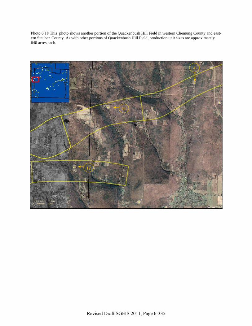
11
12
Photo 6.18 This photo shows another portion of the Quackenbush Hill Field in western Chemung County and east-ern Steuben County. As with other portions of Quackenbush Hill Field, production unit sizes are approximately 640 acres each.
4
Revised Draft SGEIS 2011, Page 6-335
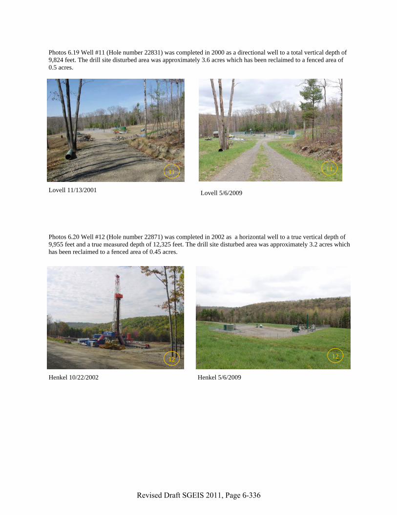
Lovell 11/13/2001 Lovell 5/6/2009
Henkel 10/22/2002 Henkel 5/6/2009
12
11
Photos 6.19 Well #11 (Hole number 22831) was completed in 2000 as a directional well to a total vertical depth of 9,824 feet. The drill site disturbed area was approximately 3.6 acres which has been reclaimed to a fenced area of 0.5 acres.
Photos 6.20 Well #12 (Hole number 22871) was completed in 2002 as a horizontal well to a true vertical depth of 9,955 feet and a true measured depth of 12,325 feet. The drill site disturbed area was approximately 3.2 acres which has been reclaimed to a fenced area of 0.45 acres.
11
12
Revised Draft SGEIS 2011, Page 6-336