Revised Better-than-BART Analysis for the Coronado

Revised Better-than-BART Analysis for the Coronado Generating Station using the CAMx

Photochemical Grid Model

Prepared for:

Salt River Project PO Box 52025

Phoenix, AZ 85072-2025

Prepared by:

Ramboll Environ US Corporation 773 San Marin Drive, Suite 2115

Novato, California, 94998 www.ramboll-environ.com

P-415-899-0700 F-415-899-0707

June 2016 06-35855C

http://www.google.com/url?sa=i&rct=j&q=&esrc=s&source=images&cd=&cad=rja&uact=8&ved=0CAcQjRxqFQoTCKy6hMS53cYCFQU5iAodS3gAtg&url=http://www.rshantz.com/Odds/General/20070827Coronado02.htm&ei=7XumVeyPMIXyoATL8IGwCw&bvm=bv.97949915,d.cGU&psig=AFQjCNHeQXb01LsyH71dZIADQsXnsW0I-g&ust=1437060445073448

June 2016

i

CONTENTS

1.0 INTRODUCTION ............................................................................................................. 1

1.1 CGS BART Analysis ........................................................................................................... 1

1.2 EPA BART Determination ................................................................................................. 1

1.3 SRP Proposed BART Alternatives ..................................................................................... 2

1.4 Document Purpose .......................................................................................................... 2

1.5 The Better-than-BART Test .............................................................................................. 3

1.5.1 Better-than-BART Test - Prong 1: No Decline in Visibility over Current Conditions at any Class I Area ............................................................................... 3

1.5.2 Better-than-BART Test - Prong 2: Overall Improvement in Visibility compared to BART control strategy ..................................................................... 4

1.6 Previous Subject-to-BART CALPUFF Modeling ................................................................ 4

1.7 Previous Better-than-BART CAMx Modeling ................................................................... 4

1.8 Report Organization ........................................................................................................ 5

2.0 DEVELOPMENT OF CAMX MODELING DATABASES .......................................................... 6

2.1 Model Selection ............................................................................................................... 6

2.2 CGS Modeling Domains ................................................................................................... 6

2.3 Meteorology .................................................................................................................... 8

2.4 Land Use ........................................................................................................................ 11

2.5 Photolysis Rates ............................................................................................................. 11

2.6 Initial and Boundary Conditions .................................................................................... 12

2.7 Emissions ....................................................................................................................... 12

2.7.1 2008 Actual Base Case Inventory ........................................................................ 12

2.7.2 2020 EPA Regional Emissions Inventory with Updates ...................................... 15

2.7.3 CGS Emission Scenarios ...................................................................................... 16

2.8 CAMx Model Performance Evaluation .......................................................................... 22

2.8.1 Model Performance Evaluation Approach ......................................................... 22

2.8.2 Total Visibility Extinction Model Performance ................................................... 24

2.8.3 Species-Specific Visibility Model Performance ................................................... 24

2.8.4 Monitor-Specific Visibility Model Performance.................................................. 27

2.8.5 Conclusions of CAMx CGS 12/4 km 2008 Base Case Model Performance ....................................................................................................... 32

2.9 CAMx CGS Better-than-BART Source Apportionment Modeling .................................. 34

June 2016

ii

2.9.1 CAMx Particulate Source Apportionment Tool (PSAT) ....................................... 34

2.9.2 CAMx PSAT Configuration ................................................................................... 34

3.0 POST-PROCESSING PROCEDURES FOR CGS CAMX MODELING ....................................... 36

3.1 Visibility Calculations using CAMx PSAT Results Following FLAG (2010) ...................... 38

3.1.1 IMPROVE Reconstructed Mass Extinction Equations ......................................... 38

3.1.2 Mapping of CAMx PSAT Species to the IMPROVE Equation Species .................. 39

3.1.3 Spatial Plots of Visibility Impacts Methodology ................................................. 40

4.0 CGS BETTER-THAN-BART RESULTS ................................................................................ 42

4.1 CGS Emission Scenarios ................................................................................................. 42

4.2 CGS Visibility Impacts .................................................................................................... 43

4.2.1 Example spatial plots for individual days ............................................................ 43

4.2.2 Delta Deciview Impacts at Class I areas .............................................................. 46

4.3 Discussions of Magnitude of Visibility Impacts ............................................................. 59

4.4 Better-than-BART Test Results ...................................................................................... 61

4.4.1 BtB1 Scenario ...................................................................................................... 63

4.4.2 BtB2 Scenario ...................................................................................................... 68

4.4.3 BtB3 Scenario ...................................................................................................... 73

4.4.4 BtB4 Scenario ...................................................................................................... 78

4.5 Conclusions of Better-than-BART Modeling.................................................................. 83

5.0 REFERENCES ................................................................................................................ 84

TABLES

Table 1-1. CGS unit 1 and unit 2 NOx and SO2 emission limits for Baseline (current), EPA BART and four SRP BtB alternative emission scenarios. ................. 2

Table 2-1. Definition of the CGS CAMx 12 and 4 km Lambert Conformation Projection (LCP) domains. ....................................................................................... 7

Table 2-2. Definition of the WRF 12/4 km modeling domains using LCP projection parameters from Table 2-1. .................................................................................... 9

Table 2-3. Vertical layer structure in WRF and CAMx. ........................................................... 10

Table 2-4. Physics options used in the WestJumpAQMS 2008 WRF simulation modeling. ............................................................................................................... 11

Table 2-5. Summary of emission sources used to develop the 2008 Actual Base Case emissions for model evaluation. ................................................................... 14

June 2016

iii

Table 2-6. CGS units 1 and 2 - diurnal emission factors by month. ....................................... 20

Table 2-7. Full load mass emission rates. ............................................................................... 21

Table 4-1. CGS emission rates and unit 1 shutdown periods for the CGS Baseline, EPA BART and four proposed alternative Better-than-BART (BtB) emission scenarios. ............................................................................................... 42

Table 4-2. CGS mass emission rates (lb/hr) for the CGS Baseline, EPA BART and four proposed alternative Better-than-BART (BtB) emission scenarios. .............. 43

Table 4-3. CGS visibility impacts from Baseline emissions..................................................... 46

Table 4-4. CGS visibility impacts from EPA BART emissions. ................................................. 48

Table 4-5. CGS visibility impacts from BtB1. .......................................................................... 51




Table 4-9. EPA BART Scenario evaluated in Prong 1 of Better-than-BART test. .................... 60

Table 4-10. Prong 1 BtB Test Summary Results ....................................................................... 61

Table 4-11. Prong 2 BtB Test Summary Results. ...................................................................... 62

Table 4-12. Prong 1 for BtB1 emissions scenario. .................................................................... 64








FIGURES

Figure 2-1. CGS CAMx 12/4 km resolution modeling domains with circle of radius 300 km centered on CGS. ........................................................................................ 8

Figure 2-2. WRF 36/12/4 km modeling domains used in the 2008 modeling. ......................... 9

Figure 2-3. Seasonal variation in heat input for CGS unit 1 and unit 2 ................................... 17

Figure 2-4. Diurnal variation of the hourly heat input rate for unit 1. .................................... 18

Figure 2-5. Diurnal variation of the hourly heat input rate for unit 2. .................................... 18

June 2016

iv

Figure 2-6. Diurnal variation of the hourly heat input rate for units 1 and 2 combined. .............................................................................................................. 19

Figure 2-7. Locations of IMPROVE monitoring sites in the CGS 4 km modeling domain where the CAMx 2008 Actual Base Case was evaluated for PM2.5 and subset of IMPROVE sites (green) where visibility evaluation was also performed. .............................................................................................. 23

Figure 2-8. Scatter plot (top) and monthly soccer plot (bottom) of 24-hour average total visibility extinction model performance across the IMPROVE sites in the 4 km CGS domain. .............................................................. 25

Figure 2-9. Soccer plots of monthly averaged visibility performance for sulfate (top left), nitrate (top right), organic aerosol (middle left), elemental carbon (middle right), soil (bottom left) and coarse mass (bottom right). ..................................................................................................................... 26

Figure 2-10. Predicted and observed 24-hour average visibility extinction and bias (Mm-1) at Petrified Forest (PEFO1) for total (top left), AmmSO4 (top right), AmmNO3 (middle left), OA (middle right), EC (bottom left) and SOIL (bottom right). ............................................................................................... 29

Figure 2-11. Predicted and observed annual average total extinction (Mm-1) stacked bar charts. ................................................................................................ 31

Figure 2-12. Predicted and observed quarterly average total extinction (Mm-1) stacked bar charts for Q1 (top left), Q2 (top right), Q3 (bottom left) and Q4 (bottom right). .......................................................................................... 32

Figure 3-1. Receptor 3x3 grid cells at IMPROVE sites and Class I areas. ................................. 37

Figure 4-1. Example single day delta deciview plume plot on February 27, 2008. ................. 44

Figure 4-2. Example single day delta deciview plume plot on May 12, 2008. ........................ 45

Figure 4-3. Spatial map of annual average delta deciview: Baseline. ..................................... 47

Figure 4-4. Spatial map of annual average delta deciview: EPA BART. ................................... 49

Figure 4-5. Spatial map of annual average delta deciview: BtB1. ........................................... 52



Figure 4-8. Spatial map of annual average delta deciview: BtB4. .......................................... 58

Figure 4-9. Spatial map of annual average Prong 1 of Better-than-BART test. BtB1. ............. 65




June 2016

v





June 2016

1

1.0 INTRODUCTION

The Salt River Project Agricultural Improvement and Power District (SRP) operates the Coronado Generating Station (CGS), a coal-fired steam electric generating station, located in Apache County, near St. Johns, Arizona. The CGS facility consists of two coal-fired units (unit 1 and unit 2) with a combined net power generating capacity of approximately 762 MW. The CGS facility became operational in 1979-1980.

1.1 CGS BART Analysis

The Clean Air Act’s Regional Haze Rule (RHR) contains a provision that each State has to address the Best Available Retrofit Technology (BART) requirements when preparing the State’s Regional Haze State Implementation Plan (SIP). A BART analysis for the CGS was performed by ENSR (2008) following the Environmental Protection Agency’s (EPA) July 6, 2005 final rule entitled “Regional Haze Regulations and Guidelines for Best Available Retrofit Technology (BART) Determinations; Final Rule” (“BART Guidelines”; EPA, 2005). The BART Guidelines include presumptive BART requirements for coal-fired electric steam generating sources greater than 750 MW.

The Arizona Department of Environmental Quality (ADEQ) determined that the CGS is a “BART-eligible source”. Based on air dispersion modeling performed by ENSR (2008), CGS is subject to BART. ENSR performed a BART analysis for the two units at CGS for two pollutants: sulfur dioxide (SO2) and oxides of nitrogen (NOx). A BART analysis was not performed for particulate matter (PM) because the hot-side electrostatic precipitators at CGS are considered to represent highly effective emission controls and because PM emissions are not a substantive contributor to regional haze in the region.

1.2 EPA BART Determination

After EPA failed to approve the BART provision in the Arizona RHR State Implementation Plan (SIP), EPA produced a Federal Implementation Plan (FIP) to define the CGS BART requirements. EPA determined1 that existing SO2 and PM emissions control at CGS satisfies BART so both CGS unit 1 and unit 2 retain the 0.08 lb/MMBtu emissions limit for SO2 emissions. A plant-wide BART limit for the averaged NOx emissions from units 1 and 2 was established as 0.065 lb/MMBtu (on a rolling 30-boiler-operating-day basis).

On April 13, 2016, EPA revised portions of the Arizona RHR FIP applicable to the CGS. In response to a petition for reconsideration from the SRP, EPA replaced a plant-wide compliance method with a unit-specific compliance method for determining compliance with the BART emission limits for NOX from units 1 and 2 at CGS. While the plant-wide limit for NOX emissions

1 http://www.epa.gov/region9/air/actions/pdf/az/haze/epa-r09-oar-2015-0165-coronado-nprm-factsheet-2015-

03-13.pdf

June 2016

2

from units 1 and 2 had been established as 0.065 lb/MMBtu, EPA has now set a unit-specific limit of 0.065 lb/MMBtu for unit 1 and 0.080 lb/MMBtu for unit 2.2

The CGS unit 2 currently can meet the 0.08 lb/MMBtu NOX emissions limit and it is presumed that CGS unit 1 could meet the 0.065 lb/MMBtu emissions limit by installing Selective Catalytic Reduction (SCR) NOX controls.

1.3 SRP Proposed BART Alternatives

On August 3, 2015, EPA finalized the Clean Power Plan (CPP)3 rulemaking to control carbon pollution from power plants to address climate change. The CPP sets state-specific goals for reducing carbon dioxide (CO2) emissions from fossil-fuel electrical generating units (EGUs). SRP is in the process of evaluating options for complying with the CPP CO2 emission reductions. In addition to evaluating options to comply with the CPP, SRP has developed alternative emission control strategies for CGS to comply with the RHR BART requirements. The SRP CGS proposed BART alternative emissions control strategies include NOX and SO2 emission limit options coupled with shutdown periods for CGS unit 1. Emissions from unit 1 of the CGS are zero during the shutdown period for all pollutants.

Table 1-1 lists the CGS unit 1 and 2 current (Baseline) SO2 and NOX emissions along with those for the EPA BART (SCR NOx controls) and the four CGS Better-than-BART (BtB) alternative emission scenarios that also include shutdown periods for CGS unit 1.

Table 1-1. CGS unit 1 and unit 2 NOx and SO2 emission limits for Baseline (current), EPA BART and four SRP BtB alternative emission scenarios.

Scenario

NOX SO2 unit 1

Shutdown Period (lb/MMBtu) (lb/MMBtu)

unit#1 unit#2 unit#1 unit#2

Baseline 0.320 0.080 0.080 0.080 None

EPA BART 0.065 0.080 0.080 0.080 None

BtB1 0.320 0.080 0.080 0.080 Oct 1 – Apr 15

BtB2 0.320 0.080 0.070 0.070 Oct 21 – Jan 31

BtB3 0.320 0.080 0.050 0.050 Nov 21 – Jan 20

BtB4 0.310 0.080 0.060 0.060 Nov 21 – Jan 20

1.4 Document Purpose

When a proposed BART alternative emissions control strategy has a different emissions distribution than the EPA BART control strategy, air quality modeling is used to quantify the visibility benefits of the proposed BART alternative strategy compared to the EPA BART strategy

2 https://www.federalregister.gov/articles/2016/04/13/2016-07911/promulgation-of-air-quality-implementation-

plans-arizona-regional-haze-federal-implementation-plan 3 http://www2.epa.gov/cleanpowerplan/clean-power-plan-existing-power-plants

June 2016

3

with the Better-than-BART test. This document presents results of the Better-than-BART modeling analysis for the CGS using the Comprehensive Air-quality Model with extensions (CAMx; www.camx.com) photochemical grid model.

1.5 The Better-than-BART Test

The requirements for demonstrating an alternative control strategy is better than a BART control strategy are outlined in EPA’s BART Guidelines (EPA, 20054). When the alternative control strategy has a different distribution of emissions, these regulations require the comparison of the modeled visibility impacts at Class I areas. EPA (2005) requires a two-pronged test to demonstrate that the proposed alternative control strategy is better than the BART control scenario (i.e., Better-than-BART):

“(t)he modeling study would demonstrate ‘greater reasonable progress’ if both of the following two criteria are met:

- Visibility does not decline in any Class I area, and

- Overall improvement in visibility, determined by comparing the average differences over all affected Class I areas.” (EPA, 2005)

To facilitate the comparisons, three emissions scenarios are evaluated: (1) Baseline scenario (current conditions); (2) the BART control scenario; and (3) the proposed alternative control scenario. Modeled visibility impacts for each scenario are calculated and compared. The comparison is performed for the observed best 20 percent (B20%) and worst 20 percent (W20%) days of the modeled year(s) for each Class I area. These days comprise the 20 % clearest and 20 % haziest days throughout a year based on observational data from the Interagency Monitoring of Protected Visual Environments network of monitors (IMPROVE5). Average visibility impacts over all B20% and W20% days are calculated and compared.

1.5.1 Better-than-BART Test - Prong 1: No Decline in Visibility over Current Conditions at any Class I Area

The difference in visibility impacts between the Baseline scenario and the proposed alternative control scenario is calculated for each Class I area for the B20% and W20% days in the modeled year. If the alternative control scenario has the same or lower visibility impacts than the Baseline scenario at all Class I areas and for both the B20% and W20% days, then “visibility does not decline in any Class I area”. Therefore, the proposed alternative control scenario passes the 1st Prong of the Better-than-BART test.

4 40 CFR Part 51 “Regional Haze Regulations and Guidelines for Best Available Retrofit Determinations” Federal

Register/ Vol. 70, No. 128/Wednesday, July 6, 2005/Rules and Regulations, pp.39104-39172. (http://www.gpo.gov/fdsys/pkg/FR-2005-07-06/pdf/05-12526.pdf). (USEPA, 2005) 5 http://vista.cira.colostate.edu/improve/

http://www.camx.com/

http://www.gpo.gov/fdsys/pkg/FR-2005-07-06/pdf/05-12526.pdf

June 2016

4

1.5.2 Better-than-BART Test - Prong 2: Overall Improvement in Visibility compared to BART control strategy

To test the 2nd Prong of the Better-than-BART test, the difference in visibility between the BART control scenario and the proposed BtB alternative control scenario is calculated. If the proposed alternative control scenario shows lower visibility impacts than the BART control scenario when averaged over all Class I areas for both the B20% and W20% days in the modeled year, then an “overall improvement in visibility” has been demonstrated. In this case, the proposed alternative control scenario passes the 2nd prong of the Better-than-BART test.

1.6 Previous Subject-to-BART CALPUFF Modeling

The CGS Subject-to-BART modeling was conducted using the CALPUFF non-steady-state Gaussian puff screening model (ENSR, 2008). CALPUFF was designated the EPA-preferred long range transport model in EPA’s 2003 modeling guidelines. However, in July 2015, EPA proposed revisions to their modeling guidelines that would delist CALPUFF as the EPA-preferred long range transport model. Instead, EPA would recommend photochemical grid models (PGMs) for applications involving secondary PM2.5 formation, including sulfate and nitrate that are the primary cause of visibility impairment in the CGS BtB modeling. Foremost among EPA’s concerns about CALPUFF is its simplistic treatment of sulfate and nitrate formation (chemistry) as CALPUFF has been shown to understate sulfate formation in summer, overstate sulfate formation in winter and overstate nitrate formation year-round (Morris et al., 2003; 2005; 2006). Given that the CGS BtB modeling trades off visibility benefits from reductions in SO2 emissions and operation (in the proposed alternative strategies) versus visibility benefits from reduced NOX emissions (BART control strategy), accurate and unbiased treatment of sulfate and nitrate formation chemistry is needed. Thus, the CGS BtB modeling is following EPA’s latest draft guidelines and using a PGM.

1.7 Previous Better-than-BART CAMx Modeling

Preliminary Better-than-BART modeling for the CGS facility was conducted with the Comprehensive Air-quality Model with extensions (CAMx) PGM. The results were documented in a Ramboll Environ (January 2016) report: “Better-than-BART Analysis for the Coronado Generating Station using the CAMx Photochemical Grid Model”. The methodologies and results were reviewed by EPA and revisions to the methodologies were requested. This report presents the results of a second round of CAMx Better-than-BART modeling in response to EPA-requested revisions. Specific revisions include: (1) use of a future year emissions CAMx modeling database instead of the 2008 base case emissions CAMx database, (2) use of temporally varying CGS emissions with seasonal and diurnal variation, (3) calculation of visibility impacts at each Class I area using an average of 3x3 receptors (grid cells) at IMPROVE sites and/or Class I area centroid locations instead of using the maximum visibility impacts from all receptors in a given Class I area, and (4) visualization of visibility impacts by presentation of spatial maps of delta deciview impacts and results of the BtB tests throughout the entire modeling domain.

June 2016

5

1.8 Report Organization

Chapter 1 presents background for the CGS BtB modeling. Development of the CAMx 2008 modeling database, and 2008 CAMx base case model performance evaluation (MPE) is contained in Chapter 2, with more details on the MPE provided in Appendix A. Chapter 3 describes the BtB tests and how the CAMx PGM modeling results were post-processed for the BtB tests. Chapter 4 presents the results of BtB tests using the CAMx modeling results from the Baseline, EPA BART, and BtB alternatives model output. References are provided in Chapter 5.

June 2016

6

2.0 DEVELOPMENT OF CAMX MODELING DATABASES

This chapter describes the development of the modeling databases for conducting the photochemical grid model (PGM) visibility assessment. Two modeling databases were used:

1. The 2008 West-wide Jump-Start Air Quality Modeling Study (WestJumpAQMS6; ENVIRON, Alpine and UNC, 20137) modeling database was used for the model performance evaluation and the previously reported preliminary Better-than-BART modeling.

2. A 2020 future year modeling database, based on the 2020 EPA emissions inventory with updates, was used for the Better-than-BART modeling presented in this report.

The Comprehensive Air-quality Model with extensions (CAMx) was used for the CGS visibility assessment for reasons listed below.

2.1 Model Selection

The CAMx PGM was selected for the CGS Better-than-BART modeling for the following reasons:

CAMx includes full science chemistry algorithms for secondary PM2.5 formation (e.g., sulfate and nitrate) that is of high importance in this application. EPA’s proposed modeling guidelines acknowledges that PGMs are generally most appropriate for addressing secondary PM2.5 which is needed for the simulation of regional visibility impairment (EPA, 2015). This is in contrast to the CALPUFF model that is recommended for Subject-to-BART screening modeling that has highly simplified chemical transformation algorithms that have been shown to have bias in sulfate and nitrate formation (Morris et al., 2003; 2005; 2006).

CAMx is one of the two PGMs mentioned in EPA’s latest modeling guidelines (EPA, 2015) and guidance (EPA, 2014d) that satisfies all the requirements for simulating secondary PM2.5 formation. CMAQ is the other PGM mentioned.

CAMx includes two-way grid nesting, which is not available in CMAQ. This is used to perform the simulation efficiently at 4 km grid cell resolution within 300 km of CGS.

CAMx includes a Plume-in-Grid module to simulate the near-source chemistry and plume dynamics that are subgrid-scale that is not included in CMAQ.

CAMx includes a mature, fully tested and evaluated Particulate Source Apportionment Technology (PSAT) tool for separately tracking the particulate matter (PM) impacts associated with emissions from CGS that is not available in CMAQ.

2.2 CGS Modeling Domains

The CAMx CGS modeling domain was chosen to provide sufficient resolution around CGS and fully encompass all Class I areas within 300 km of CGS. The study area used for the CGS Better-than-BART modeling is a nested 12 and 4 km horizontal resolution modeling domain encompassing CGS. The domain is based on the same Lambert Conformal Projection (LCP) as

6 http://www.wrapair2.org/WestJumpAQMS.aspx

7 http://www.wrapair2.org/pdf/WestJumpAQMS_FinRpt_Finalv2.pdf

June 2016

7

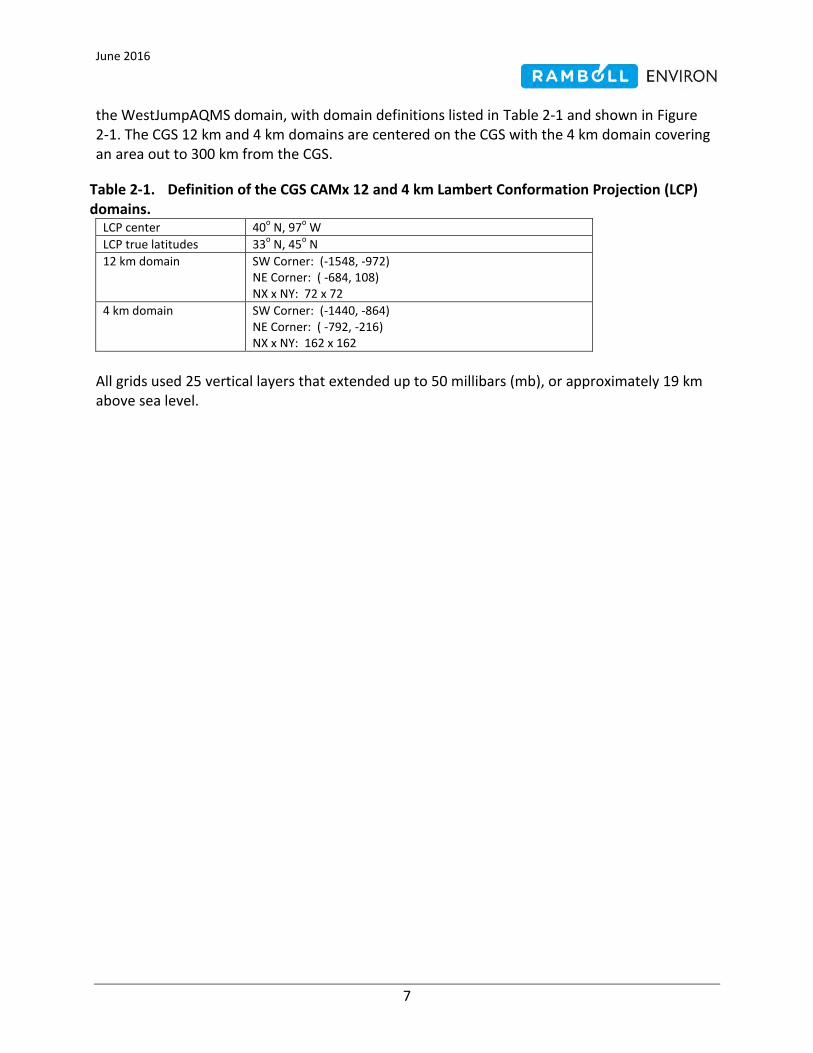
the WestJumpAQMS domain, with domain definitions listed in Table 2-1 and shown in Figure 2-1. The CGS 12 km and 4 km domains are centered on the CGS with the 4 km domain covering an area out to 300 km from the CGS.

Table 2-1. Definition of the CGS CAMx 12 and 4 km Lambert Conformation Projection (LCP) domains.

LCP center 40o N, 97

o W

LCP true latitudes 33o N, 45

o N

12 km domain SW Corner: (-1548, -972) NE Corner: ( -684, 108) NX x NY: 72 x 72

4 km domain SW Corner: (-1440, -864) NE Corner: ( -792, -216) NX x NY: 162 x 162

All grids used 25 vertical layers that extended up to 50 millibars (mb), or approximately 19 km above sea level.

June 2016

8

Figure 2-1. CGS CAMx 12/4 km resolution modeling domains with circle of radius 300 km centered on CGS.

Class I areas that are wholly or partially within 300 km of CGS were evaluated for visibility impacts. The CGS CAMx 12/4 km modeling domain shown in Figure 2-1 includes a ring of 300 km around the CGS source and displays all Class I areas within the 12/4 km modeling domain. If any part of a Class I area is included within 300 km of CGS, the visibility impacts were evaluated at that Class I area. For example, Grand Canyon National Park has only a small portion of the Class I area within 300 km of the CGS, but the entire Class I area was still included in the visibility assessment. However, Class I areas like Zion, Canyonlands, Weminuche, White Mountain and others that completely reside more than 300 km from CGS were not included in the visibility assessment.

2.3 Meteorology

The CGS Better-than-BART visibility assessment used meteorology generated by the prognostic Weather Research and Forecast (WRF) meteorological model (Skamarock et al., 2004; 2005;

June 2016

9

2006) that was applied as part of the WestJumpAQMS study (ENVIRON and Alpine, 20128). Version 3.3.1 of WRF was used in WestJumpAQMS to generate the CAMx meteorological input files for the 2008 calendar year (PGMs, due to their complexity, are typically run with only one year of modeled meteorology). WRF was configured with a 36/12/4 km nested domain structure using the LCP projection parameters given in Table 2-2 and extent shown in Figure 2-2. WRF was run with 37 vertical layers up to 50 mb (approximately 19 km above sea level) that were collapsed to 25 CAMx layers as shown in Table 2-3. The same meteorological data was used for the Better-than-BART CAMx modeling with the 2020 EPA emissions inventory with updates. All CAMx simulations used identical meteorological input files.

Table 2-2. Definition of the WRF 12/4 km modeling domains using LCP projection parameters from Table 2-1.

LCP center 40o N, 97

o W

LCP true latitudes 33o N, 45

o N

12 km domain (-2448, -1404) to ( 612, 1620) 255 x 252

4 km domain (-1632, -984) to (-156, 1236) 369 x 555

Figure 2-2. WRF 36/12/4 km modeling domains used in the 2008 modeling.

8 http://www.wrapair2.org/pdf/WestJumpAQMS_2008_Annual_WRF_Final_Report_February29_2012.pdf

June 2016

10

Table 2-3. Vertical layer structure in WRF and CAMx.

WRF Meteorological Model CAMx Air Quality Model

WRF Layer Sigma

Pressure (mb)

Approx. Height

(m) Thickness

(m) CAMx Layer

Approx. Height

(m) Thickness

(m)

37 0.0000 50.00 19260 2055 25 19260.0 3904.9

36 0.0270 75.65 17205 1850

35 0.0600 107.00 15355 1725 24 15355.1 3425.4

34 0.1000 145.00 13630 1701

33 0.1500 192.50 11930 1389 23 11929.7 2569.6

32 0.2000 240.00 10541 1181

31 0.2500 287.50 9360 1032 22 9360.1 1952.2

30 0.3000 335.00 8328 920

29 0.3500 382.50 7408 832 21 7407.9 1591.8

28 0.4000 430.00 6576 760

27 0.4500 477.50 5816 701 20 5816.1 1352.9

26 0.5000 525.00 5115 652

25 0.5500 572.50 4463 609 19 4463.3 609.2

24 0.6000 620.00 3854 461 18 3854.1 460.7

23 0.6400 658.00 3393 440 17 3393.4 439.6

22 0.6800 696.00 2954 421 16 2953.7 420.6

21 0.7200 734.00 2533 403 15 2533.1 403.3

20 0.7600 772.00 2130 388 14 2129.7 387.6

19 0.8000 810.00 1742 373 13 1742.2 373.1

18 0.8400 848.00 1369 271 12 1369.1 271.1

17 0.8700 876.50 1098 177 11 1098.0 176.8

16 0.8900 895.50 921 174 10 921.2 173.8

15 0.9100 914.50 747 171 9 747.5 170.9

14 0.9300 933.50 577 84 8 576.6 168.1

13 0.9400 943.00 492 84

12 0.9500 952.50 409 83 7 408.6 83.0

11 0.9600 962.00 326 82 6 325.6 82.4

10 0.9700 971.50 243 82 5 243.2 81.7

9 0.9800 981.00 162 41 4 161.5 64.9

8 0.9850 985.75 121 24

7 0.9880 988.60 97 24 3 96.6 40.4

6 0.9910 991.45 72 16

5 0.9930 993.35 56 16 2 56.2 32.2

4 0.9950 995.25 40 16

3 0.9970 997.15 24 12 1 24.1 24.1

2 0.9985 998.58 12 12

1 1.0000 1000 0 0

June 2016

11

Physics options used in the WestJumpAQMS 2008 WRF modeling are provided in Table 2-4. Detailed information on the WRF WestJumpAQMS application including a model performance evaluation can be found in the WestJumpAQMS WRF Application/Evaluation Report (ENVIRON and Alpine, 2012).

Table 2-4. Physics options used in the WestJumpAQMS 2008 WRF simulation modeling.

WRF Treatment Option Selected Notes Microphysics Thompson scheme New with WRF 3.1.

Longwave Radiation RRTMG Rapid Radiative Transfer Model for Global Circulation Models includes random cloud overlap and improved efficiency over RRTM.

Shortwave Radiation RRTMG Same as above, but for shortwave radiation.

Land Surface Model (LSM) NOAH Two-layer scheme with vegetation and sub-grid tiling.

Planetary Boundary Layer (PBL) scheme

YSU Yonsie University (Korea) Asymmetric Convective Model with non-local upward mixing and local downward mixing.

Cumulus parameterization Kain-Fritsch in the 36 km and 12 km domains. None in the 4 km domain.

4 km can explicitly simulate cumulus convection so parameterization not needed.

Analysis nudging Nudging applied to winds, temperature and moisture in the 36 km and 12 km domains

Temperature and moisture nudged above PBL only.

Observation Nudging Nudging applied to surface wind only in the 4 km domain

Surface temperature and moisture observation nudging can introduce instabilities.

Initialization Dataset 12 km North American Model (NAM)

Also used in analysis nudging

2.4 Land Use

The CGS 12 and 4 km resolution land use files were based on United States Geological Survey (USGS) Geographic Information Retrieval and Analysis System (GIRAS) data. These files contain the fraction of land cover in each of the 26 land use categories in the dry deposition scheme of Zhang et al. (2001; 2003) used by CAMx . In addition, monthly leaf area indices in each grid cell were prepared for the Zhang deposition scheme.

2.5 Photolysis Rates

The CAMx photolysis rates file is a lookup table of photolysis rates under clear sky conditions for a range of ozone column values, albedo, solar zenith angles, and heights above ground. Global and daily ozone column data were obtained from the database of space-based measurements from the Ozone Monitoring Instrument (OMI) on the Aura satellite (http://ozoneaq.gsfc.nasa.gov/OMIOzone.md) and processed for the 12 and 4 km domains

http://ozoneaq.gsfc.nasa.gov/OMIOzone.md

June 2016

12

using the O3MAP program. The Tropospheric Ultraviolet and Visible (TUV; NCAR, 2011) radiative transfer model developed by NCAR used ozone column outputs and appropriate chemical mechanism to calculate the photolysis rates.

2.6 Initial and Boundary Conditions

CAMx initial and boundary conditions (IC/BCs) for the CGS 12/4 km domain (Figure 2-1) were prepared by extracting hourly atmospheric concentrations of all modeled pollutants. The 2008 MPE CAMx simulation used IC/BCs from WestJumpAQMS 36 km CONUS and 12 km WESTUS 3-dimensional CAMx model outputs. The future year Better-than-BART CAMx simulations used IC/BCs from 3-dimensional model outputs of a 36 km CAMx simulation based on the 2020 EPA emissions inventory with updates.

2.7 Emissions

Emissions inputs were prepared for the CAMx 12/4 km CGS modeling domains shown in Figure 2-1 for multiple CAMx simulations. The first simulation was used for a model performance evaluation (MPE) to establish confidence in the model for this application. For this simulation the emissions were taken directly from the WestJumpAQMS emissions inventory and are referred to as the Actual 2008 Base Case emissions. This database was originally developed as part of the Western Regional Air Partnership (WRAP) West-wide Jump-Start Air Quality Modeling Study (WestJumpAQMS9; ENVIRON, Alpine and UNC, 201310) and then adopted by the Western Air Quality Study (WAQS, Adelman, Shanker, Yang and Morris, 2014) and is available on the Intermountain West Data Warehouse (IWDW11). The WestJumpAQMS website contains detailed documentation of the study including modeling plans and protocols, the meteorological model evaluation, technical memorandums detailing the emissions and the final report. The inventory is summarized in the following section but note that the CGS emissions for the Actual 2008 Base Case simulation were hour-specific from the 2008 Continuous Emissions Monitoring (CEM) database.

Preliminary Better-than-BART CAMx modeling was performed with the WestJumpAQMS database , and the results were documented in a Ramboll Environ (January 2016) report: “Better-than-BART Analysis for the Coronado Generating Station using the CAMx Photochemical Grid Model”. The results presented in this report are based on CAMx simulations with various BtB emissions scenarios using regional emissions based on the 2020 EPA emissions inventory with updates as requested by EPA that are described in Section 2.7.2. 2.7.1 2008 Actual Base Case Inventory

The 2008 Actual Base Case emissions inventory were used for the CAMx 2008 12/4 km base case simulation that was used in the model performance evaluation. The 2008 WestJumpAQMS emission inventory formed the framework for these data. The primary source for the 2008

9 http://www.wrapair2.org/WestJumpAQMS.aspx

10 http://www.wrapair2.org/pdf/WestJumpAQMS_FinRpt_Finalv2.pdf

11 http://views.cira.colostate.edu/tsdw/

June 2016

13

WestJumpAQMS emission was the 2008 National Emission Inventory, version 2 (2008 NEIv2.012).

Table 2-5 summarizes the sources of data and methods used to develop the 2008 base case emissions. The 2008 Actual Base Case emissions are based on the 2008 NEIv2.0 with the following improvements:

Emissions of SO2 and NOX from major Electrical Generating Units (EGUs) (i.e., those exceeding 25 MW), including CGS, were obtained from 2008 Continuous Emissions Monitor (CEM) measurement data that are available from the EPA Clean Air Markets Division (CAMD13). These data are hour-specific for SO2, NOx and heat input. The temporal variability of other pollutant emissions (e.g., PM and VOC) for the CEM sources were estimated using the hourly CEM heat input data to allocate the annual emissions from the 2008 NEIv2.0 to each hour of the year. Emissions, locations and stack parameters for point sources without CEM devices were based on the 2008 NEIv2.0.

The WRAP-IPAMS Phase III 2006 oil and gas emission inventories that WestJumpAQMS projected to 2008 were used in the emissions development. In addition, WestJumpAQMS developed new 2008 oil and gas emissions inventory for the Permian Basin in southern New Mexico and northwestern Texas. The CGS 12/4 km domain also includes portions of the WRAP 2008 oil and gas emissions for the North and South San Juan and Permian Basins.

On-road mobile source emissions were derived from the MOVES on-road mobile source emissions model.

The WRAP windblown dust (WBD) model14 was used to generate WBD emissions using day-specific hourly meteorology from the 2008 WRF simulation.

Sea salt and lightning emissions were generated using the 2008 WRF model hourly gridded output.

Emissions from fires (wildfires, prescribed burns and agricultural burning) were based on the 2008 fire emissions inventory developed in the Joint Fire Sciences Program (JFSP) Deterministic and Empirical Assessment of Smoke’s Contribution to Ozone (DEASCO315) study (Moore et al., 2011). Fire emissions were assumed to be constant across all scenarios.

Biogenic emissions were generated using an enhanced version of MEGAN that was updated by WRAP to better represent biogenic emissions for the western states. Biogenic emissions will be assumed constant across all scenarios.

Mexico emissions were based on the 2008 projections from the 1999 Mexico national emissions inventory.

The Environment Canada 2006 emissions inventory based on the National Pollutant Release Inventory (NPRI) were used for Canada.

12

http://www.epa.gov/ttn/chief/net/2008inventory.html 13

http://www.epa.gov/airmarkets 14

http://www.wrapair.org/forums/dejf/fderosion.html 15

https://wraptools.org/pdf/ei_methodology_20130930.pdf

http://www.wrapair.org/forums/dejf/fderosion.html

June 2016

14

New spatial surrogates for the emissions developed using the latest 2010 Census and other data that are now available were used in emissions modeling. Details on the new spatial surrogates used for allocating county-level emissions to the 4 km grid cells can be found in the WestJumpAQMS Emissions Technical Memorandum Number 13 (available at http://www.wrapair2.org/pdf/Memo13_Parameters_Sep30_2013.pdf).

The 2008 Actual Base Case emissions are fully documented in 16 Technical Memorandums that are available on the WestJumpAQMS website16.

Table 2-5. Summary of emission sources used to develop the 2008 Actual Base Case emissions for model evaluation.

Emissions Component Configuration Details

Oil and Gas Emissions

Update WRAP Phase III 2006 to 2008

Seven WRAP Phase III Basins in CO, NM, UT and WY plus add 2008 Permian Basin O&G Emissions

Area Source Emissions

2008 NEI Version 2.0 Western state updates, then SMOKE processing of http://www.epa.gov/ttn/chief/net/2008inventory.html

On-Road Mobile Sources

MOVES MOVES 2008 emissions run in inventory mode

Point Sources 2008 CEM and Non-CEM Sources

Use 2008 day-specific hourly measured CEM for SO2 and NOX emissions for CEM sources, 2008 NEIv2.0 for other pollutants and non-CEM sources

Off-Road Mobile Sources

2008 NEIv2.0 Based on EPA NONROAD model http://www.epa.gov/oms/nonrdmdl.htm

Wind Blown Dust Emissions

WRAP Wind Blown Dust (WBD)

WRAP WBD Model with 2008 WRF meteorology adjusted to be consistent with 2002 WBD modeling

Ammonia Emissions

NEIv2.0 Based on CMU Ammonia Model. Review and update spatial allocation if appropriate.

Biogenic Sources

MEGAN

Enhanced version of MEGAN Version 2.1 from WRAP Biogenics study http://www.wrapair2.org/pdf/WGA_BiogEmisInv_FinalReport_March20_2012.pdf

Fires 2008 DEASCO3 2008 DEASCO3 fire inventory used. https://wraptools.org/pdf/ei_methodology_20130930.pdf

Temporal Adjustments

Seasonal, day, hour Based on latest collected information

Chemical Speciation

CB6r2 Chemical Speciation

Revision 2 of the Carbon Bond Version 6 chemical mechanism

Gridding Spatial Surrogates based on land use

Develop new spatial surrogates using 2010 census data and other data

Quality Assurance

SMOKE QA Tools; PAVE, VERDI plots; Summary reports

Follow WRAP emissions QA/QC plan.

16

http://www.wrapair2.org/WestJumpAQMS.aspx

http://www.wrapair2.org/pdf/Memo13_Parameters_Sep30_2013.pdf

http://www.epa.gov/ttn/chief/net/2008inventory.html

http://www.epa.gov/oms/nonrdmdl.htm

http://www.wrapair2.org/pdf/WGA_BiogEmisInv_FinalReport_March20_2012.pdf


https://wraptools.org/pdf/ei_methodology_20130930.pdf

http://www.wrapair2.org/WestJumpAQMS.aspx

June 2016

15

2.7.2 2020 EPA Regional Emissions Inventory with Updates

The regional inventory that was used to develop the future year emissions scenario for the Better-than-BART CAMx modeling is described in this section. The 2020 EPA emissions inventory used for the PM NAAQS Rule (available at http://www.epa.gov/ttn/chief/emch) formed the framework of the future year regional emissions. The 2020 EPA emission inventory is based on the 2007 PM NAAQS emissions database which in turn is based on the 2008 NEI.

The 2020 EPA emissions inventory represents projected emissions with promulgated Federal and State control measures. It reflects projected economic changes and fuel usage for EGU and mobile sectors. The 2020 EGU projected inventory represents demand growth, fuel resource availability, generating technology cost and performance, and other economic factors affecting power sector behavior. It also reflects the expected 2020 emissions effects due to environmental rules and regulations, consent decrees and settlements, plant closures, control devices updated since 2007, and forecast unit construction through the calendar year 2020. The projected EGU emissions include the Final Mercury and Air Toxics (MATS) rule announced on December 21, 2011 and the Final Cross-State Air Pollution Rule (CSAPR) issued on July 6, 2011. For the future year emissions scenarios, the following emission categories were assumed to remain unchanged from the 2008 base case emissions scenario:

Biogenic emissions.

Fire emissions.

Lightning emissions.

Sea salt emissions.

Windblown dust emissions.

Emissions from Mexico and Canada.

2.7.2.1 Updates to 2020 EPA Regional Emissions Inventory

Oil and gas emissions were updated from the 2020 EPA inventory to account for additional reasonably foreseeable development (RFD). The RFD is defined as: 1) air emissions from the undeveloped portions of authorized NEPA projects and Resource Management Plans (RMPs), and 2) air emissions from not-yet-authorized NEPA projects (if emissions are quantified when emissions modeling commences). These sources are in addition to regional sources present in the 2020 EPA emissions inventory.

http://www.epa.gov/ttn/chief/emch

June 2016

16

2.7.3 CGS Emission Scenarios

For the CAMx simulations, the following CGS emission scenarios were modeled:

1. CGS Baseline conditions that represents current emissions conditions at the facility; 2. CGS EPA BART that represents CGS with the EPA BART NOX emission limits; and 3. Several CGS proposed alternative emission scenarios (herein referred to as BtB scenarios)

that have specific emission limits along with shutdown periods for CGS unit 1. One of EPA’s recommendations for the updated CGS CAMx Better-than-BART (BtB) modeling was to incorporate seasonal and diurnal variability into the modeled CGS unit 1 and 2 emissions. This would make the BtB modeling more similar to Regional Haze SIP Photochemical Grid Model (PGM) analyses. The varying “emission scalars” would be applied not only to the baseline emissions of all modeled species, but also to the EPA BART scenario and the Better-than-BART alternatives.

In order to develop these emission scalars, CGS unit 1 and 2 daily and hourly heat input data were analyzed from EPA's Acid Rain database for the 5 year period (2006-2010) centered on the BART analysis 2008 baseline year. This data was averaged across the five years and plotted to examine the typical seasonal and diurnal variations in heat input rates and resulting mass emission rates.

Figure 2-3 examines the seasonal variation in heat input for the units. This plot presents the total heat input rates for units 1 and 2 and both units combined for each day in the year, averaged across the 5 year period. Also plotted are the moving 30 day averages. The day averages do not include days with very low heat input rates (less than 26,000 MMBtu/day, equal to about 20% load), since those days represent startup/shutdown days and not normal operating days (there were only 70 boiler operating days excluded during the entire 5 year data period). Figure 2-3 indicates that there is some day to day variability throughout the year, and there is a reduced operating level for the period from approximately May through June. The data plot also indicates that on average, the daily utilization of units 1 and 2 are essentially equal and are on the order of 83% to 89%, indicating these are base load units with high utilization.

June 2016

17

Figure 2-3. Seasonal variation in heat input for CGS unit 1 and unit 2

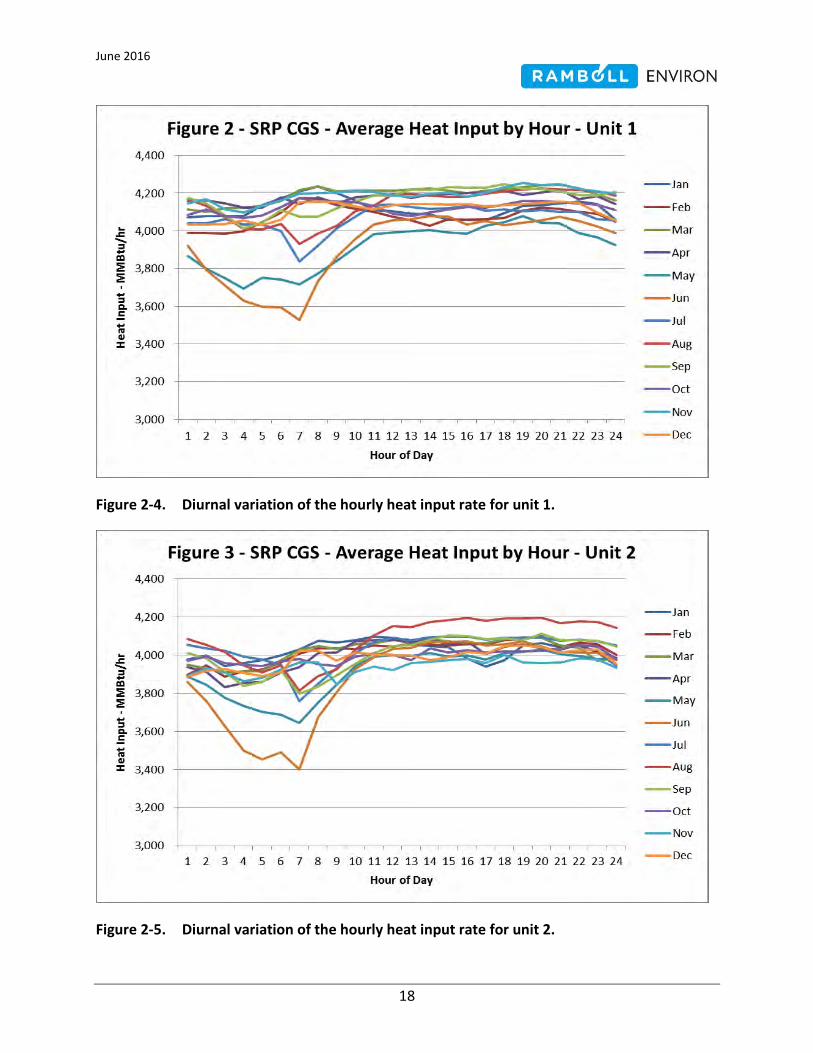
Figure 2-4 through Figure 2-6 present the diurnal variation of the hourly heat input rate for units 1 and 2 separately and combined, by month of the year. Once again, these hour averages are across the five year period 2006-2010 and do not include hours with low heat input rates (less than 471 MMBtu/hr), which reflect startup/shutdown operations and are not representative of normal operation; there were only 566 hours with heat input rates between 0 and 471 MMBtu/hr that were excluded during the 5 year (43,824 hour) data period. Figure 2-4 and Figure 2-5 indicate that the hourly average heat input rates for the two units are very similar. Figure 2-6 indicates that the heat input to the two units combined is relatively uniform after approximately 11 am, however in the morning hours there is somewhat lower utilization, particularly for the months of May and June and to some extent during July and August.

June 2016

18

Figure 2-4. Diurnal variation of the hourly heat input rate for unit 1.

Figure 2-5. Diurnal variation of the hourly heat input rate for unit 2.

June 2016

19

Figure 2-6. Diurnal variation of the hourly heat input rate for units 1 and 2 combined.

Using this heat input data, the diurnally varying emission scalars for each hour in the day and each month in the year were calculated and are presented in Table 2-6. These have been calculated based on the heat input for the two units combined divided by the maximum combined hourly capacity of 9,438 MMBtu/hr. The emission scalars vary over a range of 0.73 for the hour of 6 am during June, to a value of 0.89 during the late afternoon and early evening hours in August.

June 2016

20

Table 2-6. CGS units 1 and 2 - diurnal emission factors by month.

The full load mass emissions for various species are presented in Table 2-7, and are based on the lb/MMBtu emission factors and a 4,719 MMBtu/hr maximum heat input rate for each unit. These full load mass emission rates were multiplied by the monthly and diurnally varying emission scalars in Table 2-6 to calculate the time varying emission rates that were input to the CAMx model.

June 2016

21

Table 2-7. Full load mass emission rates.

SRP Scenario unit

lb/MMBtu Emissions in pounds per hour

SO2 Rate

NOx Rate SO2 SO4 NOX HNO3 NO3 PMF PMC EC SOA

Baseline 1 0.08 0.32 377.5 1.89 1,510.1 0 0 59.03 80.27 2.3 0

2 0.08 0.08 377.5 12.4 377.5 0 0 59.03 80.27 2.3 0

EPA BART 1 0.08 0.065 377.5 12.4 306.7 0 0 59.03 80.27 2.3 0

2 0.08 0.08 377.5 12.4 377.5 0 0 59.03 80.27 2.3 0

BtB1 1 0.08 0.32 377.5 1.89 1,510.1 0 0 59.03 80.27 2.3 0

2 0.08 0.08 377.5 12.4 377.5 0 0 59.03 80.27 2.3 0

BtB2 1 0.07 0.32 330.3 1.89 1,510.1 0 0 59.03 80.27 2.3 0

2 0.07 0.08 330.3 12.4 377.5 0 0 59.03 80.27 2.3 0

BtB3 1 0.05 0.32 236.0 1.89 1,510.1 0 0 59.03 80.27 2.3 0

2 0.05 0.08 236.0 12.4 377.5 0 0 59.03 80.27 2.3 0

BtB4 1 0.06 0.31 283.1 1.89 1,462.9 0 0 59.03 80.27 2.3 0

2 0.06 0.08 283.1 12.4 377.5 0 0 59.03 80.27 2.3 0 Notes:

The maximum heat input rate for each unit is 4719 MMBtu/hr

The combined PMF and PMC filterable emissions are equal to the consent decree PM limit of 0.03 lb/MMBtu, or 141.57 lb/hr

The PMF fraction of total PM10 is 43.30% based on AP-42 Table 1.1-6

Elemental Carbon is 3.7% of PMF, based on an analysis contained in SRP's BART Report.

Sulfate emissions for non-SCR scenarios are calculated using SRP stack test emission factor of 0.0004 lb/MMBtu.

Sulfate emissions for SCR scenarios are calculated using EPRI Method. Based on Coronado coal characteristics , the SCR scenario sulfate emissions are estimated at 12.4 lb/hr, equal to 0.0026 lb/MMBtu

The effective total PM10 emission rate when including condensible sulfate emissions is 0.0326 lb/MMBtu

June 2016

22

2.8 CAMx Model Performance Evaluation

The WestJumpAQMS and Western Air Quality Study (WAQS) CAMx 2008 base case modeling results were subjected to one of the most detailed and comprehensive model performance evaluations (MPE) ever conducted. The results of the MPE are documented in the WestJumpAQMS final report (ENVIRON, Alpine and UNC, 2013) and the WAQS report (Adelman, Shanker, Yang and Morris, 201417). Since the focus of this study is to assess visibility impacts only, the MPE for the CGS CAMx 2008 12/4 km Actual Base Case simulation focused on the model’s ability to simulate PM2.5 total mass, PM2.5 individual species mass, and species specific visibility extinctions only. The MPE will rely on the WestJumpAQMS and WAQS model evaluations for the other components.

In this section we present a summary of the evaluation of the CGS 2008 12/4 km Actual Base Case simulation for visibility. Additional details are provided in Appendix A.

2.8.1 Model Performance Evaluation Approach

The CGS CAMx 2008 12/4 km Actual Base Case was evaluated by comparing the model’s PM2.5 and visibility predictions at IMPROVE sites in the CGS 4 km domain as shown in Figure 2-7. The predicted and observed PM2.5 species and NO2 concentrations were converted to visibility extinction using the latest IMPROVE equation and Class I area-specific relative humidity adjustment factors [f(RH)] following the procedures in FLAG (2010). The total and species-specific PM2.5 mass and visibility extinction model performance statistics were compared against established PM Performance Goals and Criteria as well as the more stringent ozone Performance Goals. In addition, numerous graphical displays of model performance were used to illustrate model performance as follows:

Scatter plots of predicted and observed total extinction with summary model performance statistics.

Soccer plots of monthly bias and error for total extinction and by species extinction that are compared against ozone performance goals and PM performance goals and criteria. Monthly soccer plots allow the easy identification of when performance goals/criteria are achieved and a seasonal evaluation of performance. Note that because we are only evaluating visibility and PM2.5, the ozone performance goals are not relevant. However, they are included on the soccer plot displays and represent very good performance for visibility and PM2.5.

Time series plots that compare predicted and observed daily total visibility extinction and by species visibility extinction at individual monitoring sites.

Stacked bar charts that compare predicted and observed annual and seasonal total visibility extinction and by species visibility extinction at individual monitoring sites.

17

http://views.cira.colostate.edu/tsdw/Documents/

June 2016

23

Spatial statistical performance maps that display bias/error on a map at the locations of the monitoring sites in order to better understand spatial attributes of model performance along with tabular summaries of statistical performance metrics. (See Appendix A).

All performance statistics and displays are performed matching the predicted and observed concentrations by time and location using the modeled prediction in the 4 km grid cell containing the monitoring site.

The model performance statistics and displays were generated using the Atmospheric Model Evaluation Tool (AMET) developed by EPA, which is the MPE tool mentioned in EPA’s latest PGM modeling guidance (EPA, 2014d). Thus, the statistics and displays are limited to those produced by AMET. AMET uses screening criteria to make sure that sufficient observations are available at a monitoring site for use in the model evaluation. Consequently, some of the IMPROVE sites are dropped from the visibility MPE.

Figure 2-7. Locations of IMPROVE monitoring sites in the CGS 4 km modeling domain where the CAMx 2008 Actual Base Case was evaluated for PM2.5 and subset of IMPROVE sites (green) where visibility evaluation was also performed.

June 2016

24

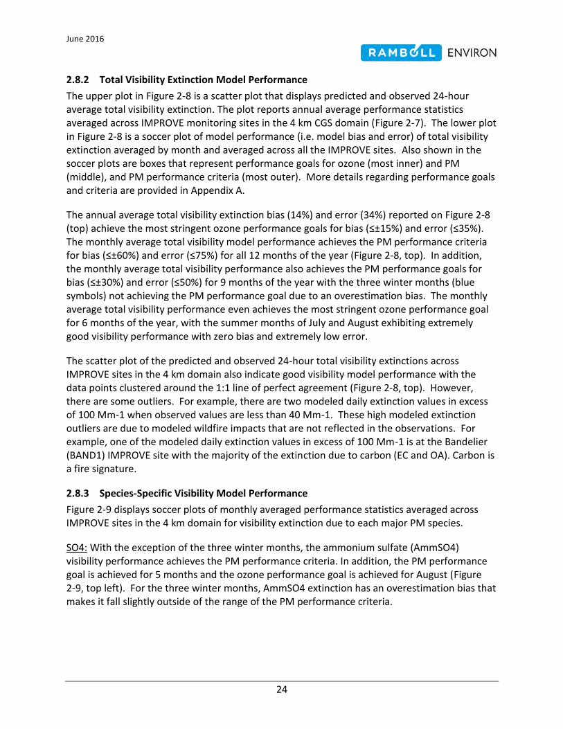
2.8.2 Total Visibility Extinction Model Performance

The upper plot in Figure 2-8 is a scatter plot that displays predicted and observed 24-hour average total visibility extinction. The plot reports annual average performance statistics averaged across IMPROVE monitoring sites in the 4 km CGS domain (Figure 2-7). The lower plot in Figure 2-8 is a soccer plot of model performance (i.e. model bias and error) of total visibility extinction averaged by month and averaged across all the IMPROVE sites. Also shown in the soccer plots are boxes that represent performance goals for ozone (most inner) and PM (middle), and PM performance criteria (most outer). More details regarding performance goals and criteria are provided in Appendix A.

The annual average total visibility extinction bias (14%) and error (34%) reported on Figure 2-8 (top) achieve the most stringent ozone performance goals for bias (≤±15%) and error (≤35%). The monthly average total visibility model performance achieves the PM performance criteria for bias (≤±60%) and error (≤75%) for all 12 months of the year (Figure 2-8, top). In addition, the monthly average total visibility performance also achieves the PM performance goals for bias (≤±30%) and error (≤50%) for 9 months of the year with the three winter months (blue symbols) not achieving the PM performance goal due to an overestimation bias. The monthly average total visibility performance even achieves the most stringent ozone performance goal for 6 months of the year, with the summer months of July and August exhibiting extremely good visibility performance with zero bias and extremely low error.

The scatter plot of the predicted and observed 24-hour total visibility extinctions across IMPROVE sites in the 4 km domain also indicate good visibility model performance with the data points clustered around the 1:1 line of perfect agreement (Figure 2-8, top). However, there are some outliers. For example, there are two modeled daily extinction values in excess of 100 Mm-1 when observed values are less than 40 Mm-1. These high modeled extinction outliers are due to modeled wildfire impacts that are not reflected in the observations. For example, one of the modeled daily extinction values in excess of 100 Mm-1 is at the Bandelier (BAND1) IMPROVE site with the majority of the extinction due to carbon (EC and OA). Carbon is a fire signature.

2.8.3 Species-Specific Visibility Model Performance

Figure 2-9 displays soccer plots of monthly averaged performance statistics averaged across IMPROVE sites in the 4 km domain for visibility extinction due to each major PM species.

SO4: With the exception of the three winter months, the ammonium sulfate (AmmSO4) visibility performance achieves the PM performance criteria. In addition, the PM performance goal is achieved for 5 months and the ozone performance goal is achieved for August (Figure 2-9, top left). For the three winter months, AmmSO4 extinction has an overestimation bias that makes it fall slightly outside of the range of the PM performance criteria.

June 2016

25

Figure 2-8. Scatter plot (top) and monthly soccer plot (bottom) of 24-hour average total visibility extinction model performance across the IMPROVE sites in the 4 km CGS domain.

June 2016

26

Figure 2-9. Soccer plots of monthly averaged visibility performance for sulfate (top left), nitrate (top right), organic aerosol (middle left), elemental carbon (middle right), soil (bottom left) and coarse mass (bottom right).

June 2016

27

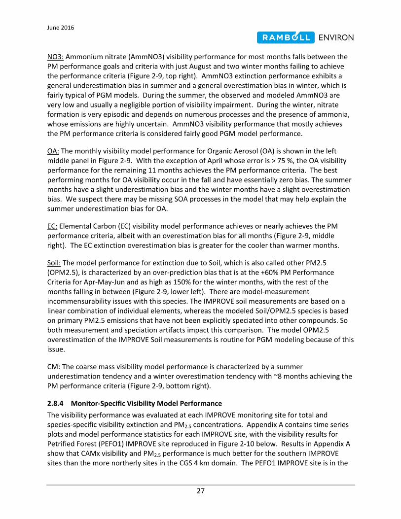
NO3: Ammonium nitrate (AmmNO3) visibility performance for most months falls between the PM performance goals and criteria with just August and two winter months failing to achieve the performance criteria (Figure 2-9, top right). AmmNO3 extinction performance exhibits a general underestimation bias in summer and a general overestimation bias in winter, which is fairly typical of PGM models. During the summer, the observed and modeled AmmNO3 are very low and usually a negligible portion of visibility impairment. During the winter, nitrate formation is very episodic and depends on numerous processes and the presence of ammonia, whose emissions are highly uncertain. AmmNO3 visibility performance that mostly achieves the PM performance criteria is considered fairly good PGM model performance.

OA: The monthly visibility model performance for Organic Aerosol (OA) is shown in the left middle panel in Figure 2-9. With the exception of April whose error is > 75 %, the OA visibility performance for the remaining 11 months achieves the PM performance criteria. The best performing months for OA visibility occur in the fall and have essentially zero bias. The summer months have a slight underestimation bias and the winter months have a slight overestimation bias. We suspect there may be missing SOA processes in the model that may help explain the summer underestimation bias for OA.

EC: Elemental Carbon (EC) visibility model performance achieves or nearly achieves the PM performance criteria, albeit with an overestimation bias for all months (Figure 2-9, middle right). The EC extinction overestimation bias is greater for the cooler than warmer months.

Soil: The model performance for extinction due to Soil, which is also called other PM2.5 (OPM2.5), is characterized by an over-prediction bias that is at the +60% PM Performance Criteria for Apr-May-Jun and as high as 150% for the winter months, with the rest of the months falling in between (Figure 2-9, lower left). There are model-measurement incommensurability issues with this species. The IMPROVE soil measurements are based on a linear combination of individual elements, whereas the modeled Soil/OPM2.5 species is based on primary PM2.5 emissions that have not been explicitly speciated into other compounds. So both measurement and speciation artifacts impact this comparison. The model OPM2.5 overestimation of the IMPROVE Soil measurements is routine for PGM modeling because of this issue.

CM: The coarse mass visibility model performance is characterized by a summer underestimation tendency and a winter overestimation tendency with ~8 months achieving the PM performance criteria (Figure 2-9, bottom right).

2.8.4 Monitor-Specific Visibility Model Performance

The visibility performance was evaluated at each IMPROVE monitoring site for total and species-specific visibility extinction and PM2.5 concentrations. Appendix A contains time series plots and model performance statistics for each IMPROVE site, with the visibility results for Petrified Forest (PEFO1) IMPROVE site reproduced in Figure 2-10 below. Results in Appendix A show that CAMx visibility and PM2.5 performance is much better for the southern IMPROVE sites than the more northerly sites in the CGS 4 km domain. The PEFO1 IMPROVE site is in the

June 2016

28

center of the 4 km domain and is fairly representative of average model performance. The exception to this is for elemental carbon (EC) extinction and concentration, where PEFO1 is the best performing site with the other IMPROVE sites exhibiting an overestimation bias for EC.

2.8.4.1 PEFO Time Series Analysis

The total extinction time series comparison at PEFO1 displays an overestimation in Q1, underestimation in Q2 and excellent performance in Q3 and Q4 (Figure 2-10, top left) resulting in very good annual model performance statistics with low bias (5%) and error (28%) that achieves the most stringent ozone performance goals. The AmmSO4 extinction at PEFO1 (Figure 2-10, top right) also has an overestimation bias in Q1 but good performance the rest of the year resulting in a positive annual bias (18%) that achieves the PM performance goal for bias and annual error (61%) that slightly exceeds the PM Performance Goal for error (≤±60%). The AmmNO3 extinction performance at PEFO1 (Figure 2-10, middle left) is fairly typical of AmmNO3 performance with the model underestimating the summer low values but overestimating the winter high values resulting in a low annual bias (4%) that achieves the ozone and PM performance goal for bias but much higher annual error (79%) that just barely exceeds the PM performance criterion for error (≤75%).

OA extinction is underestimated in Q2 and Q3 resulting in an annual bias (-30 %) that is equal to the PM performance goal and an annual error (42%) that achieves the PM performance goal (Figure 2-10, middle right). The EC extinction performance at PEFO1 is the best of any IMPROVE site with near zero bias (2%) and low error (33%) that achieves the most stringent ozone performance goals (Figure 2-10, bottom left). Note that EC extinction performance at all the other IMPROVE sites in the 4 km domain exhibit an overestimation bias of 23% to 79%. Soil extinction is overestimated except during Q2 with an annual bias value at PEFO1 of 127%, which is fairly typical (Figure 2-10, bottom right). As noted previously, the IMPROVE equation defines Soil using a linear combination of atmospheric elements differently than how the model defines this species. Although not included in Figure 2-6, but reported in Appendix A, extinction due to coarse mass at PEFO1 is underestimated (-24%) and achieves the PM performance goal with the error (73%) just achieving the PM performance criterion.

June 2016

29

Figure 2-10. Predicted and observed 24-hour average visibility extinction and bias (Mm-1) at Petrified Forest (PEFO1) for total (top left), AmmSO4 (top right), AmmNO3 (middle left), OA (middle right), EC (bottom left) and SOIL (bottom right).

June 2016

30

2.8.4.2 Annual Average and Quarterly Average Speciated Extinction Performance by Monitor

Figure 2-11 displays stacked bar charts of annual average total extinction at each IMPROVE site with the stacked bars showing each PM2.5 component of extinction. For most sites, the observed and predicted annual average total extinction are similar, although the modeled annual average total extinction tends to be the same or slightly higher than the observed value. Annual average AmmSO4 extinction agrees well at all IMPROVE sites. The annual AmmNO3 extinction also agrees well at most sites, although some have an annual overestimation bias (e.g., MEVE1) and others have an annual underestimation (e.g., SAGU1) bias. The predicted and observed annual average extinction due to OA (OC) are very similar. The model tends to overestimate extinction due to EC. The model consistently overstates the amount of extinction due to Soil at all sites. Finally, the annual average extinction comparison of coarse mass shows an overestimation bias at some sites (e.g., BAND1) and an underestimation bias at other sites (e.g., SYCA1). The site with the highest annual total overestimation bias is BAND1 whose overestimation is primarily due to overstated extinction due to EC, Soil and coarse mass that is partly due to modeled wildfire contributions that were not as large in the observations.

Stacked extinction bar charts by quarter are shown in Figure 2-12 that clearly show variations in the CAMx visibility model performance by quarter and by species. The modeled annual average extinction overestimation is primarily due to overstated extinction across several species in Q1 and Q4. The model extinction performance in Q2 and Q3 is quite good at all monitoring sites.

June 2016

31

Figure 2-11. Predicted and observed annual average total extinction (Mm-1) stacked bar charts.

June 2016

32

Figure 2-12. Predicted and observed quarterly average total extinction (Mm-1) stacked bar charts for Q1 (top left), Q2 (top right), Q3 (bottom left) and Q4 (bottom right).

2.8.5 Conclusions of CAMx CGS 12/4 km 2008 Base Case Model Performance

The CAMx total visibility extinction achieves the PM performance goal on an annual average basis as well as for 9 months of the year. The overestimation bias in winter months results in model performance falling between the PM performance goals and performance criteria levels for the other 3 months.

Visibility performance varies geographically, seasonally and by PM species. As shown in Appendix A, the visibility model performance at IMPROVE sites in the lower two-thirds of the 4 km CGS modeling domain is quite good at meeting the most stringent ozone performance goals, whereas the visibility model performance at IMPROVE sites in the top third of the domain have an overestimation bias, but still achieve the PM performance goals except at the Bandelier (BAND1) IMPROVE site. Part of the reason that the model overestimates visibility extinction at

June 2016

33

the BAND1 IMPROVE site is because of modeled impacts from wildfires that were not as high in the observations.

The seasonal total visibility model performance shows very good performance for the warmer months (e.g., Q2 and Q3) and an overestimation bias for the cooler months (e.g., Q1 and Q4). The monthly total visibility model performance achieves the PM performance criteria for all months, the PM performance goal for 9 months and the ozone performance goal for 7 months.

The ammonium sulfate (AmmSO4) and ammonium nitrate (AmmNO3) visibility performance is fairly good with 9 months achieving the PM performance criteria. AmmSO4 visibility performance also has many months achieving the PM performance goal.

Visibility performance due to organic aerosol is fairly good, albeit with a summer underestimation bias. And visibility performance for elemental carbon and soil generally exhibit an overestimation bias.

The main objective of the CGS Better-than-BART visibility modeling is to evaluate the trade-offs of visibility benefits between reducing CGS’s NOX versus SO2 emissions. The visibility performance for AmmSO4 and AmmNO3 is good and mostly unbiased and the bias that does occur (slight winter overestimation) is common to both AmmSO4 and AmmNO3. Given this, and the fact that CAMx incorporates state-of-the-science sulfate and nitrate formation chemistry algorithms, the CAMx 2008 12/4 km CGS modeling platform should provide an accurate and reliable database for evaluating and comparing visibility impacts of the BART modeling scenarios and proposed alternative control scenarios.

June 2016

34

2.9 CAMx CGS Better-than-BART Source Apportionment Modeling

CAMx was applied for CGS Baseline emissions, CGS EPA BART emissions, and proposed CGS BtB alternative emissions using the 12/4 km modeling domain, 2008 meteorological conditions and 2020 EPA regional emissions with updates for all other sources. The CAMx Particulate Source Apportionment Technology (PSAT) Probing Tool was used to separately track contributions of particulate matter (PM) and reactive gaseous nitrogen (RGN) concentrations (which include NO2) due to SO2, NOX and PM emissions from the CGS units.

2.9.1 CAMx Particulate Source Apportionment Tool (PSAT)

The PSAT source apportionment tool uses reactive tracers (also called tagged species) that run in parallel to the host model to determine the contributions to PM from user selected Source Groups. A Source Group is a tagged group of emissions sources whose impacts are separately tracked using the reactive tracers. Source Groups are usually defined as the intersection between geographic Source Regions (e.g., grid cell definitions of states) and user selected Source Categories (e.g., point, on-road mobile, etc.). However, for the CGS CAMx source apportionment modeling, the Source Groups will consist of the two CGS units and all other natural and anthropogenic emissions.

The CAMx PSAT particulate source apportionment method has five different families of tracers that can be invoked separately or together to track source apportionment for the following particulate species: (1) Sulfate (SO4); (2) Nitrate and Ammonium (NO3 and NH4); (3) Primary PM; (4) Secondary Organic Aerosol (SOA); and (5) Mercury. Because PSAT needs to track the PM source apportionment from the PM precursor emissions to the PM species, the number of tracers needed to track a Source Group’s source apportionment depends on the complexity of the chemistry and number of PM and intermediate species involved. The Sulfate family is the most simple as it requires only two reactive tracer species (SO2 and SO4) to track the formation of particulate SO4 from gaseous SO2 emission for each Source Group. Whereas, the SOA family is the most complicated (expensive) PSAT family with 18 reactive tracers needed for each Source Group to track the four VOC species emissions that are SOA precursors (aromatics, isoprene, terpenes and sesquiterpenes) and the 7 condensable gas (CG) and SOA pairs that are in equilibrium.

For the CAMx CGS Better-than-BART source apportionment application, the PSAT SO4, NO3/NH4, and Primary PM families of source apportionment tracers were used. The PSAT SOA family of source apportionment was not used because the CGS EGU units do not emit any VOC species that are SOA precursors.

2.9.2 CAMx PSAT Configuration

SO2, NOX and primary PM emissions from the CGS units were tagged for treatment by the PSAT tool for each of the emission scenarios. For the CGS baseline and CGS BART simulations, CAMx was run with 3 source groups representing: CGS unit 1; CGS unit 2; and, all other emissions sources.

June 2016

35

For the proposed alternative emission simulation BtB1, CAMx was run with 16 source groups. One source group represented non-CGS emissions, another represented unit 2 CGS emissions and the other 14 source groups represented the unit 1 CGS emissions for different time periods as follows:

January and February combined (1 group)

March and April ~ 15 day periods each (4 groups)

May, June, July, August as individual months (4 groups)

September and October ~ 15 day periods each (4 groups)

November and December combined (1 group)

Performing the CAMx simulations for the proposed alternative emission simulation BtB1 with CGS unit 1 tagged separately for different periods enables evaluation of the CGS proposed alternative visibility impacts using different CGS unit 1 shutdown assumptions without having to rerun CAMx. Preliminary CAMx simulations indicated that for the BtB1 alternative emissions scenario, the required shutdown period would include all of November through February as well as additional time periods, therefore January and February were tagged together and November and December were tagged together.

For the other three proposed alternative emission simulations BtB2, BtB3, and BtB4, CAMx was run with 18 source groups. One source group represented non-CGS emissions, another represented unit 2 CGS emissions and the other 16 source groups represented the unit 1 CGS emissions for different time periods as follows:

January 1 to March 10 (~ 10 day periods) (7 groups)

March 11 to June 30 (1 groups)

July 1 to October 20 (1 groups)

October 21 – December 31 (~ 10 day periods (7 groups)

Performing the CAMx simulations for the proposed alternative emission simulations BtB2, BtB3, BtB4 with CGS unit 1 tagged separately for ~10 day periods between October 21 and March 10 enabled evaluation of the CGS proposed alternative visibility impacts using different CGS unit 1 shutdown assumptions at 10-day increments without having to rerun CAMx.

June 2016

36

3.0 POST-PROCESSING PROCEDURES FOR CGS CAMX MODELING

Visibility impacts attributed to the CGS for baseline, EPA BART and proposed alternative emission scenarios were calculated at all Class I areas. The differences in visibility impacts between the different scenarios were then compared in the Better-than-BART two-pronged tests that were described in Section 1.5.

Visibility impacts were calculated based on the CAMx absolute modeled concentrations using incremental CGS concentrations as quantified by the CAMx PSAT tool in the IMPROVE extinction equation (described below). FLAG (2010) procedures were followed. The change in light extinction due to CGS emissions was calculated for each day for grid cells associated with Class I areas within 300 km of the CGS facility. The average visibility impact over a 3x3 grid cell array centered at: (1) the IMPROVE monitor associated with the Class I area, or (2) the centroid of the Class I area (if there was no associated IMPROVE site) was used to represent the visibility impact at that Class I area. The grid cells used are presented in Figure 3-1. The IMPROVE monitor name is shown on the map in yellow, and Class I area names are displayed in green italics. Results for all the Class I areas labelled on the figure are reported. Processing the CAMx concentrations to obtain visibility impacts using this method gives visibility impacts similar to those determined by CALPUFF, except that they are based on modeled results from a full-science model. In addition, calculating the average visibility on a 3x3 array of grid cells is similar to methodologies used by the EPAs Modeled Attainment Test Software (MATS18).

Two averaging approaches were taken to calculate the visibility impacts. The first approach averages the visibility impacts across the W20% and B20% days, the second approach performs the averaging across all modeled days which provides an annual average assessment of visibility impacts.

18

http://www3.epa.gov/ttn/scram/modelingapps_mats.htm

June 2016

37

Figure 3-1. Receptor 3x3 grid cells at IMPROVE sites and Class I areas.

June 2016

38

3.1 Visibility Calculations using CAMx PSAT Results Following FLAG (2010)

The visibility evaluation metric used in this analysis is based on the Haze Index which is measured in deciview (dv) units and is defined as follows:

HI = 10 x ln[bext/10] .

bext is the atmospheric light extinction reported in inverse megameters (Mm-1) and is calculated primarily from atmospheric concentrations of particulates. The incremental concentrations due to CGS emissions was added to natural background concentrations in the extinction equation (bext) and the difference between the Haze Index with added CGS concentrations to the Haze Index based solely on background concentrations was calculated. This quantity is the change in

Haze Index, which is referred to as “delta deciview” (dv):

Δdv = 10 x ln[bext(CGS+background)/10] - 10 x ln[bext(background)/10]

Δdv = 10 x ln[bext(CGS+background)/bext(background)]

Here bext(CGS+background) refers to atmospheric light extinction due to emissions from CGS plus natural background concentrations, and bext(background) refers to atmospheric light extinction due to natural background concentrations only. In Section 4, delta deciview impacts are referred to more simply as CGS visibility impacts.

3.1.1 IMPROVE Reconstructed Mass Extinction Equations

The FLAG (2010) procedures for evaluating visibility impacts at Class I areas use the revised IMPROVE reconstructed mass extinction equation to convert PM species in μgm-3 to light extinction (bext) in inverse megameters (Mm-1) as follows:

bext = bSO4 + bNO3 + bEC + bOCM + bSoil + bPMC+ bSeaSalt+ bRayleigh+ bNO2

where

bSO4 = 2.2 × fS(RH) × [Small Sulfate] + 4.8 × fL(RH) × [Large Sulfate]

bNO3 = 2.4 × fS(RH) × [Small Nitrate] + 5.1 × fL(RH) × [Large Nitrate]

bOCM = 2.8 × [Small Organic Mass] + 6.1 × [Large Organic Mass]

bEC = 10 × [Elemental Carbon]

bSoil = 1 × [Fine Soil]

bPMC = 0.6 × [Coarse Mass]

bSeaSalt = 1.7 × fSS(RH) × [Sea Salt]

June 2016

39

bRayleigh = Rayleigh Scattering (Site-specific)

bNO2 = 0.33 × [NO2 (ppb)] {or as: 0.1755 × [NO2 (μg/m3)]}.

f(RH) are relative humidity adjustment factors that account for the fact that sulfate, nitrate, organic aerosol and sea salt aerosols are hygroscopic and are more effective at scattering radiation at higher relative humidity. FLAG (2010) recommends using monthly average f(RH) values rather than the hourly averages recommended in the previous FLAG (2000) guidance document in order to moderate the effects of extreme weather events on the visibility results. The Class I area-specific monthly average f(RH) values from Tables 7 through 9 from FLAG (2010) will be used.

The revised IMPROVE equation treats “large sulfate” and “small sulfate” separately because large and small aerosols affect an incoming beam of light differently. However, the IMPROVE measurements do not separately measure large and small sulfate; they measure only the total PM2.5 sulfate. Similarly, CAMx writes out a single concentration of particulate sulfate for each grid cell. Part of the definition of the new IMPROVE equation is a procedure for calculating the large and small sulfate contributions based on the magnitude of the model output sulfate concentrations; the procedure is documented in FLAG (2010). The sulfate concentration magnitude is used as a surrogate for distinguishing between large and small sulfate concentrations. For a given grid cell, the large and small sulfate contributions are calculated from the model output sulfate (which is the “Total Sulfate” referred to in the FLAG (2010) guidance) as:

For Total Sulfate < 20 μg/m3:

[Large Sulfate] = ([Total Sulfate] / 20 μg/m3) × [Total Sulfate]

For Total Sulfate ≥ 20 μg/m3:

[Large Sulfate] = [Total Sulfate]

For all values of Total Sulfate:

[Small Sulfate] = [Total Sulfate] – [Large Sulfate]

The procedure is identical for nitrate and organic mass. The split between Large and Small Sulfate is based on the Total Sulfate concentrations from the model. We assume that the incremental Sulfate concentrations due to just emissions from CGS have the same split between Large and Small Sulfate concentrations as the modeled Total Sulfate concentration.

3.1.2 Mapping of CAMx PSAT Species to the IMPROVE Equation Species

The CAMx PSAT source apportionment runs provide incremental concentration contributions due to CGS emissions for the following species that will be used in the revised IMPROVE equation discussed above:

June 2016

40

Sulfate (SO4)

Nitrate (NO3)

Elemental Carbon (EC)

Primary Organic Aerosol (POA, used for Organic Mass)

Fine Crustal (FCRS) and Other (FPRM) primary PM2.5 emissions (used for Soil).

Coarse Crustal (CCRS) and Other (CPRM) coarse (PM2.5-10) PM species (used for CM or PMC)

Reactive Gaseous Nitrogen (RGN, used for NO2)

The CGS incremental sulfate and nitrate concentrations will be assumed to be completely neutralized by ammonium.

The PSAT source apportionment algorithm does not separately track NO2 concentrations but instead tracks total reactive nitrogen (RGN) that consists mainly of NO, NO2 and other smaller mass reactive nitrogen species (e.g., N2O5, NO3 radical, etc.). The CGS incremental concentrations of the PSAT RGN species were used to represent light extinction due to NO2. This may overstate the CGS visibility impairment associated with NO2. In terms of the Better-than-BART test, this assumption will be conservative by overstating the visibility reductions in the EPA BART scenario relative to the proposed BtB alternative scenario since the EPA BART scenario has more NOX emission reductions. In any event, the vast majority of visibility impairment due to emissions from CGS is due to ammonium sulfate and ammonium nitrate and the treatment of NO2 in the visibility calculations has a minimal impact.

Although sodium and particulate chloride are treated in the CAMx core model, these species are not carried in the CAMx PSAT tool; neglecting sea salt in the visibility calculations in the CGS visibility assessment does not compromise the accuracy of the analysis as IMPROVE measurements show that sea salt concentrations are negligible in this inland area and there are no sodium or chloride emissions associated with the CGS units.

3.1.3 Spatial Plots of Visibility Impacts Methodology

In addition to tabulated results of the Better-than-BART tests at the individual Class I areas, software was developed to produce spatial plots of annual average delta deciviews across the entire CAMx 4 km modeling domain as well as spatial plots of the annual average Prong 1 and Prong 2 of the Better-than-BART test. These plots are to aid understanding of the small delta deciview values and to provide assurance that the small numbers are not numerical “noise” but do represent actual visibility impacts.

The calculation of visibility impacts for the spatial plots follows the same methodology that is outlined above. Annual average results are presented in the spatial plots. Note that the B20% days and W20% days are based on different sets of days at each Class I area (and B20% and W20% days are not defined for grid cells outside of the Class I areas), plotting regional variations in B20% days and W20% days impacts would result in inconsistent time periods being

June 2016

41

plotted for the various grid cells, which would make the analysis less useful. Note that domain-wide average values were used for relative humidity adjustment factors (f(RH)) and background concentrations in the spatial plots, rather than Class I area-specific values, in order to simplify the processing and avoid discontinuities across Class I area boundaries. Therefore the plot results are not expected to agree exactly with the tabulated result, but differences will be small.

June 2016

42

4.0 CGS BETTER-THAN-BART RESULTS

The Better-than-BART tests were applied for four proposed alternative emission scenarios for CGS using the CAMx absolute modeling results for the Baseline, EPA BART and four proposed BtB alternative emission scenarios.

4.1 CGS Emission Scenarios

Six separate CGS emissions scenarios were modeled as described in Section 2.7.3. Table 4-1 summarizes the six CGS emission scenarios modeled by CAMx in this analysis. Throughout this chapter the proposed alternative emissions scenarios are referred to as Better-than-BART (BtB) scenarios numbered 1 – 4, based on the emission rates and shutdown periods shown in Table 4-1. The CGS baseline scenario represents current emissions, note that the proposed alternative emissions scenario BtB1 is based on the same emissions and has a shutdown period of October 1 to April 15. The EPA BART emissions scenario has a lower CGS unit 1 NOX emissions rate (0.065 lb/MMBtu) than all other emission scenarios (0.320-0.310 lb/MMBtu). The proposed alternative emissions scenarios BtB2, BtB3 and BtB4 have lower SO2 emissions rates (0.070, 0.050 and 0.060 lb/MMBtu, respectively) for CGS units 1 and 2 than the Baseline, EPA BART, and BtB1 scenarios (0.080 lb/MMBtu).

Table 4-1. CGS emission rates and unit 1 shutdown periods for the CGS Baseline, EPA BART and four proposed alternative Better-than-BART (BtB) emission scenarios.

Scenario

NOX SO2

unit 1 Shutdown Period

(lb/MMBtu) (lb/MMBtu)

unit#1 unit#2 unit#1 unit#2

Baseline 0.320 0.080 0.080 0.080 None

EPA BART 0.065 0.080 0.080 0.080 None

BtB1 0.320 0.080 0.080 0.080 Oct 1 – Apr 15

BtB2 0.320 0.080 0.070 0.070 Oct 21 – Jan 31

BtB3 0.320 0.080 0.050 0.050 Nov 21 – Jan 20

BtB4 0.310 0.080 0.060 0.060 Nov 21 – Jan 20

The proposed alternative emission scenarios (BtB1, BtB2, BtB3, and BtB4) have been developed to improve upon the visibility benefits of the EPA BART NOX reductions by obtaining greater benefits in visibility due to lower SO2 emissions and the CGS unit 1 shutdown periods.

Table 4-2 shows the full load hourly mass emission rates for the six CGS emission scenarios while the CGS is operating. Note that these mass emissions rates are multiplied by the monthly and diurnal emissions scalars in Table 2-6 to calculate the time varying emission rates that were input to the CAMx model. The hourly emissions for the Baseline and BtB1 emission scenarios are the same although the annual emissions will be different as CGS unit 1 is shut down for six and a half months. The EPA BART unit 1 NOX emissions are reduced by approximately 79% from the Baseline level, which is assumed to be due to implementation of Selective Catalytic

June 2016

43

Reduction (SCR) post-combustion emissions control technology. The use of SCR will also increase primary sulfate emissions.

Table 4-2. CGS mass emission rates (lb/hr) for the CGS Baseline, EPA BART and four proposed alternative Better-than-BART (BtB) emission scenarios.

SRP Scenario unit

CGS Emissions in pounds per hour

SO2 SO4 NOX HNO3 NO3 PMF PMC EC SOA

Baseline 1 377.5 1.89 1,510.1 0 0 59.03 80.27 2.3 0

2 377.5 12.4 377.5 0 0 59.03 80.27 2.3 0

EPA BART 1 377.5 12.4 306.7 0 0 59.03 80.27 2.3 0

2 377.5 12.4 377.5 0 0 59.03 80.27 2.3 0

BtB1 1 377.5 1.89 1,510.1 0 0 59.03 80.27 2.3 0

2 377.5 12.4 377.5 0 0 59.03 80.27 2.3 0

BtB2 1 330.3 1.89 1,510.1 0 0 59.03 80.27 2.3 0

2 330.3 12.4 377.5 0 0 59.03 80.27 2.3 0

BtB3 1 236.0 1.89 1,510.1 0 0 59.03 80.27 2.3 0

2 236.0 12.4 377.5 0 0 59.03 80.27 2.3 0

BtB4 1 283.1 1.89 1,462.9 0 0 59.03 80.27 2.3 0

2 283.1 12.4 377.5 0 0 59.03 80.27 2.3 0

4.2 CGS Visibility Impacts

Visibility impacts due to emissions from the two CGS units at each Class I area are presented in this section.

4.2.1 Example spatial plots for individual days

This section provides spatial maps of visibility impacts on 2 example days to visualize the extent of visibility impairment plumes over the modeling domain.

Figure 4-1 and Figure 4-2 show delta deciview impact plume plots for the CGS Baseline (top left), EPA BART (top right), BtB1 (middle left), BtB2 (middle right), BtB3 (bottom left) and BtB4 (bottom right) emissions scenarios over the entire CAMx 4 km modeling domain for February 27 and May 12, respectively. The transport wind directions are different on these two days, therefore different Class I areas are impacted by CGS. More Class I areas are impacted under the easterly winds on February 27 than under the south-westerly winds observed on May 12.

For the February 27 plots, the BtB1 emissions scenario has zero emissions from unit 1 on that day, therefore, the CGS impacts under the BtB1 scenario are the lowest of all the emissions scenarios. February 27 shows a more dispersed plume than on May 12. For the May 12 plots, the CGS impact plume only overlaps two Class I areas, and the plume impacts at the two Class I areas are similar for all the emission cases.

June 2016

44

Figure 4-1. Example single day delta deciview plume plot on February 27, 2008.

June 2016

45

Figure 4-2. Example single day delta deciview plume plot on May 12, 2008.

June 2016

46

4.2.2 Delta Deciview Impacts at Class I areas

Table 4-3 presents CGS visibility impacts (i.e., delta deciview impacts described in Section 3.1) from the CGS Baseline emissions averaged over the B20% days, W20% days, and all days in 2008. Maximum impacts for all three time-averaged methods are reported at Petrified Forest NP (0.0406 dv) which is the Class I area located closest to the CGS facility.

Figure 4-3 is a spatial plot of the annual average delta deciview impacts for the Baseline CGS emissions scenario. The domain was defined so that the CGS facility is located approximately in the center of the modeling domain. Annual average delta deciview impacts are highest close to CGS facility and decrease with distance away from the facility. The rate of decrease varies depending on the direction, for example annual average delta decivews east of the CGS facility are in general higher than annual average delta decivews west of the facility.

Table 4-3. CGS visibility impacts from Baseline emissions.

Delta Dv

Average Best 20% Days*

Average Worst 20% Days*

Annual Average

Class I Area Absolute (dv) Absolute (dv) Absolute (dv)

Bandalier NM 0.0063 0.0170 0.0096

Bosque 0.0063 0.0049 0.0104

Chiricahua NM 0.0081 0.0015 0.0040

Chiricahua Wild 0.0092 0.0015 0.0041

Galiuro Wild 0.0051 0.0016 0.0031

Gila Wild 0.0151 0.0030 0.0140

Grand Canyon NP 0.0006 0.0030 0.0044

Mazatzal Wild 0.0167 0.0039 0.0053

Mesa Verde NP 0.0013 0.0063 0.0071

Mount Baldy Wild 0.0209 0.0172 0.0226

Petrified Forest NP 0.0087 0.0147 0.0406

Pine Mountain Wild 0.0133 0.0025 0.0052

Saguro NP 0.0041 0.0013 0.0023

San Pedro Parks Wild 0.0080 0.0134 0.0126

Sierra Ancha Wild 0.0087

Superstition Wild 0.0224 0.0027 0.0060

Sycamore Canyon Wild 0.0058 0.0037 0.0050

Maximum 0.0224 0.0172 0.0406

Cumulative (sum) 0.1521 0.0982 0.1649

Average 0.0095 0.0061 0.0097

Minimum 0.0006 0.0013 0.0023

* Best and Worst Days of Monitored visibility, from MATS (IMPROVE) database, some sites/years lack data

June 2016

47

Figure 4-3. Spatial map of annual average delta deciview: Baseline.

June 2016

48

Table 4-4 reports the CGS visibility impacts from the CGS EPA BART emissions averaged over the

B20% days, W20% days, and all days in 2008. Figure 4-4 is a spatial plot of the annual average

delta deciview impacts for the EPA BART CGS emissions scenario.

Table 4-4. CGS visibility impacts from EPA BART emissions. Case: EPA_BART_R3

Delta Dv



Annual Average


Bandalier NM 0.0050 0.0138 0.0077

Bosque 0.0052 0.0040 0.0085

Chiricahua NM 0.0060 0.0014 0.0033

Chiricahua Wild 0.0069 0.0014 0.0034

Galiuro Wild 0.0041 0.0014 0.0025

Gila Wild 0.0121 0.0026 0.0113

Grand Canyon NP 0.0004 0.0024 0.0039

Mazatzal Wild 0.0127 0.0033 0.0043

Mesa Verde NP 0.0011 0.0055 0.0064

Mount Baldy Wild 0.0171 0.0137 0.0175



Saguro NP 0.0034 0.0012 0.0019





Maximum 0.0184 0.0138 0.0346

Cumulative (sum) 0.1213 0.0806 0.1368

Average 0.0076 0.0050 0.0080

Minimum 0.0004 0.0012 0.0019

* Best and Worst Days of Monitored visibility, from MATS (IMPROVE) database, some sites/years lack data.

June 2016

49

Figure 4-4. Spatial map of annual average delta deciview: EPA BART.

June 2016

50

Table 4-5, Table 4-6, Table 4-7, and Table 4-8 report CGS visibility impacts from the CGS proposed alternative BtB1, BtB2, BtB3, and BtB4 emissions scenarios, respectively, averaged over the B20% days, W20% days, and all days in 2008.

Annual average CGS visibility impacts averaged over all class I areas for the BtB scenarios range from 0.0074 to 0.0080 dv. The corresponding CGS Baseline impact is 0.0097 dv and the corresponding CGS EPA BART impact is 0.0080 dv. For annual average visibility impacts, all CGS BtB emissions scenarios show lower visibility impacts than the CGS EPA BART scenario.

The evaluation of the Better-than-BART two-prong test using these calculated visibility impacts is presented in Section 4.4.

Figure 4-5, Figure 4-6, Figure 4-7, and Figure 4-8 present spatial plots of annual average delta deciview impacts for the BtB1, BtB2, BtB3, and Bt4 CGS emissions scenarios, respectively.

Differences between the four BtB scenarios are subtle and difficult to discern in this spatial representation. This is because the annual average delta deciview values are similar on each grid cell for all BtB emissions scenarios. Differences between the four scenarios are more easily discernible in the Prong 2 test plots presented in Section 4.4.

June 2016

51

Table 4-5. CGS visibility impacts from BtB1. Case: BtB1_R4

Delta Dv



Annual Average


Bandalier NM 0.0039 0.0118 0.0074

Bosque 0.0040 0.0039 0.0083

Chiricahua NM 0.0051 0.0015 0.0032

Chiricahua Wild 0.0057 0.0015 0.0033

Galiuro Wild 0.0035 0.0016 0.0024

Gila Wild 0.0092 0.0029 0.0109

Grand Canyon NP 0.0004 0.0029 0.0033

Mazatzal Wild 0.0105 0.0038 0.0039

Mesa Verde NP 0.0008 0.0050 0.0054

Mount Baldy Wild 0.0128 0.0145 0.0174



Saguro NP 0.0033 0.0011 0.0017





Maximum 0.0137 0.0145 0.0316

Cumulative (sum) 0.0949 0.0801 0.1260

Average 0.0059 0.0050 0.0074

Minimum 0.0004 0.0011 0.0017 * Best and Worst Days of Monitored visibility, from MATS (IMPROVE) database, some sites/years lack data.

June 2016

52

Figure 4-5. Spatial map of annual average delta deciview: BtB1.

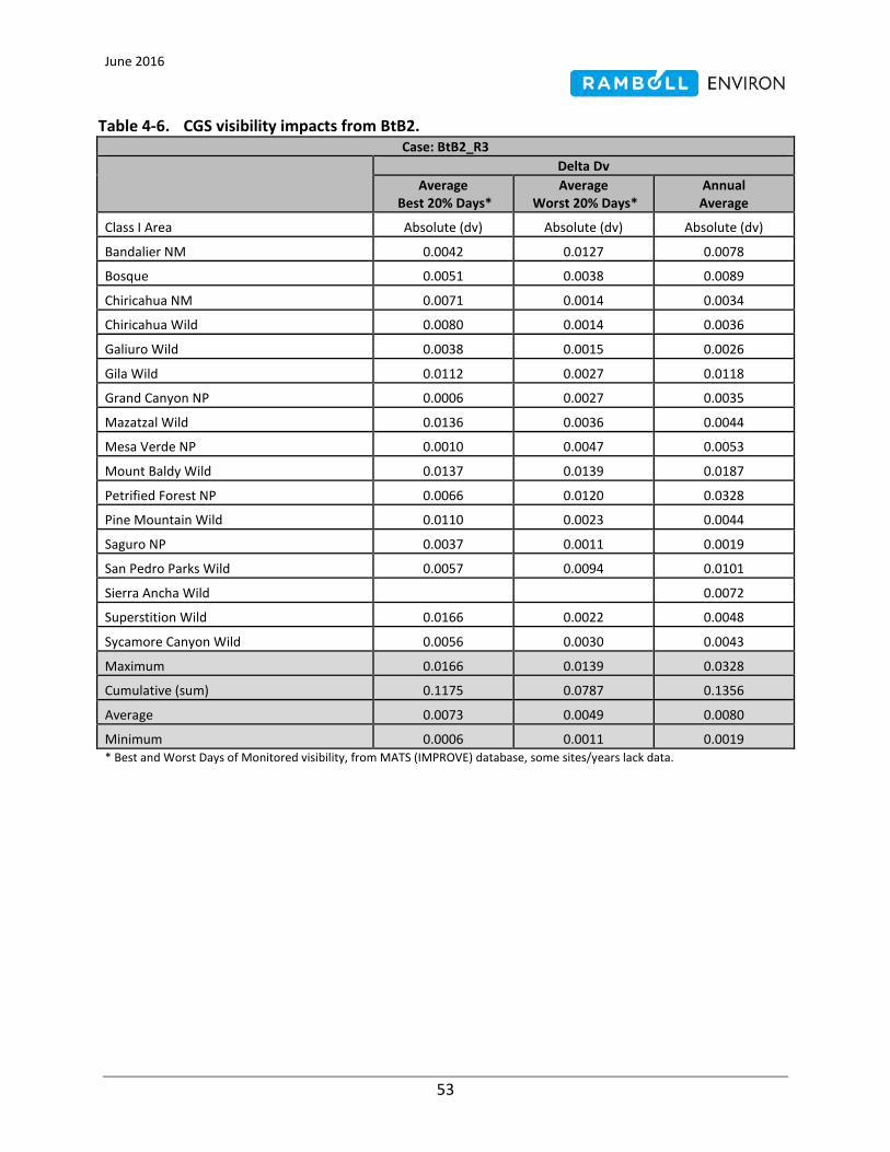
June 2016

53


Delta Dv



Annual Average


Bandalier NM 0.0042 0.0127 0.0078

Bosque 0.0051 0.0038 0.0089

Chiricahua NM 0.0071 0.0014 0.0034

Chiricahua Wild 0.0080 0.0014 0.0036

Galiuro Wild 0.0038 0.0015 0.0026

Gila Wild 0.0112 0.0027 0.0118

Grand Canyon NP 0.0006 0.0027 0.0035

Mazatzal Wild 0.0136 0.0036 0.0044

Mesa Verde NP 0.0010 0.0047 0.0053

Mount Baldy Wild 0.0137 0.0139 0.0187



Saguro NP 0.0037 0.0011 0.0019





Maximum 0.0166 0.0139 0.0328

Cumulative (sum) 0.1175 0.0787 0.1356

Average 0.0073 0.0049 0.0080


June 2016

54


June 2016

55


Delta Dv



Annual Average


Bandalier NM 0.0042 0.0120 0.0071

Bosque 0.0047 0.0034 0.0081

Chiricahua NM 0.0067 0.0011 0.0031

Chiricahua Wild 0.0075 0.0011 0.0032

Galiuro Wild 0.0035 0.0012 0.0023

Gila Wild 0.0108 0.0023 0.0110

Grand Canyon NP 0.0005 0.0023 0.0032

Mazatzal Wild 0.0142 0.0031 0.0042

Mesa Verde NP 0.0009 0.0047 0.0049

Mount Baldy Wild 0.0141 0.0148 0.0183



Saguro NP 0.0031 0.0010 0.0017





Maximum 0.0157 0.0148 0.0326

Cumulative (sum) 0.1146 0.0757 0.1287

Average 0.0072 0.0047 0.0076


June 2016

56


June 2016

57


Delta Dv



Annual Average


Bandalier NM 0.0042 0.0127 0.0076

Bosque 0.0049 0.0036 0.0086

Chiricahua NM 0.0069 0.0013 0.0033

Chiricahua Wild 0.0078 0.0013 0.0034

Galiuro Wild 0.0037 0.0013 0.0025

Gila Wild 0.0111 0.0025 0.0115

Grand Canyon NP 0.0006 0.0025 0.0035

Mazatzal Wild 0.0140 0.0033 0.0044

Mesa Verde NP 0.0010 0.0052 0.0054

Mount Baldy Wild 0.0139 0.0155 0.0191



Saguro NP 0.0034 0.0011 0.0018





Maximum 0.0164 0.0155 0.0338

Cumulative (sum) 0.1169 0.0804 0.1356

Average 0.0073 0.0050 0.0080


June 2016

58


June 2016

59

4.3 Discussions of Magnitude of Visibility Impacts

In this section the magnitude of CGS visibility impacts and the differences between the Baseline and alternative BtB scenarios impacts (i.e. Prong 1 of the Better-than-BART test) is put into context. To provide this context, the EPA BART scenario is evaluated in Prong 1 of the Better-than-BART test to examine the visibility improvements that would be expected from the EPA BART NOX SCR emissions controls compared to current (Baseline) conditions.

As reported in Section 4.2, the largest CGS visibility impact calculated at any Class I area for any of the emissions scenarios and for any time averaging method is the annual average visibility impact at Petrified Forest National Park (NP) for the Baseline emission scenario with a visibility impact of 0.0406 dv. Note that 1.0 dv is a small but perceptible scenic change under a wide range of visibility conditions19 that is “just perceptible to the human eye”20. Given that the Better-than-BART tests evaluate differences between small CGS visibility impacts, the differences between impacts are even smaller deciview values (potentially nearly an order of magnitude smaller again). It is difficult to assign significance to these very small delta deciview differences between the Baseline and EPA BART versus the Better-than-BART alternative scenarios. Therefore, in addition to absolute delta deciview differences, relative percent differences are also presented in the Better-than-BART tests.

Table 4-9 presents the results of the Prong 1 evaluation of the EPA BART emissions scenario. Note that this information is provide for context only and is not part of the Better-than-BART test. The minimum absolute delta deciview differences over all Class I areas range from 0.0002 dv to 0.0003 dv for the three averaging methods. The minimum percent differences range from 7.22 % to 9.91% for the three averaging methods. The magnitude of the Prong 1 test results for the EPA BART emission scenario will be compared to the BtB Prong 1 test results in the next section.

19

http://www3.epa.gov/ttnamti1/files/ambient/visible/tracking.pdf 20

http://www3.epa.gov/ttn/scram/11thmodconf/IWAQM3_LRT_Report-07152015.pdf

June 2016

60

Table 4-9. EPA BART Scenario evaluated in Prong 1 of Better-than-BART test. Prong 1 of BtB Test (Case Provided for Context)

Case: Baseline_R3 - EPA BART_R3

Class I Area

Delta Dv Differences

Average Average

Annual Average Best 20% Days Worst 20% Days

Absolute

Relative

Absolute

Relative

Absolute

Relative (dv) (dv) (dv)

Bandalier NM 0.0012 19.44% 0.0032 18.84% 0.0019 19.49%

Bosque 0.0011 17.66% 0.0009 19.12% 0.0019 17.89%

Chiricahua NM 0.0021 25.57% 0.0002 10.50% 0.0007 18.33%

Chiricahua Wild 0.0023 24.67% 0.0002 9.91% 0.0008 18.18%

Galiuro Wild 0.0009 18.41% 0.0002 13.77% 0.0005 17.94%

Gila Wild 0.0031 20.31% 0.0004 11.92% 0.0027 19.47%

Grand Canyon NP 0.0002 26.24% 0.0006 19.28% 0.0005 12.10%

Mazatzal Wild 0.0040 24.00% 0.0006 16.38% 0.0009 17.73%

Mesa Verde NP 0.0002 14.32% 0.0007 11.64% 0.0007 9.27%

Mount Baldy Wild 0.0038 18.34% 0.0035 20.49% 0.0050 22.24%

Petrified Forest NP 0.0006 7.22% 0.0031 20.71% 0.0060 14.78%

Pine Mountain Wild 0.0030 22.72% 0.0003 10.04% 0.0008 14.45%

Saguro NP 0.0007 16.98% 0.0002 11.85% 0.0003 14.46%

San Pedro Parks Wild 0.0019 24.16% 0.0027 19.88% 0.0027 21.33%

Sierra Ancha Wild 0.0012 13.88%

Superstition Wild 0.0040 17.92% 0.0006 20.45% 0.0010 15.95%

Sycamore Canyon Wild 0.0016 26.89% 0.0005 13.72% 0.0006 11.20%

Minimum 0.0002 7.22% 0.0002 9.91% 0.0003 9.27%

June 2016

61

4.4 Better-than-BART Test Results

Table 4-10 displays the results of Prong 1 of the Better-than-BART test for the four proposed alternative BtB emissions scenarios with shutdown periods. This first prong of the Better-than-BART test examines the differences in visibility impacts (delta dv) between the Baseline and the proposed alternative BtB scenarios (Baseline - BtB). The BtB scenario passes if the difference in visibility impact is positive or zero for all Class I areas for the W20% and B20% days. Also reported are differences in visibility impacts averaged over all 365 modeled days.

The results in Table 4-10 show the minimum differences in visibility impacts across all Class I areas between the Baseline and the proposed alternative BtB scenarios. Since the minimum differences are all positive, the proposed alternative BtB scenarios exhibit visibility improvements compared to current conditions at all Class I areas. Therefore the proposed alternative BtB scenarios with the specified shutdown periods show “Visibility does not decline in any Class I area” and hence the BtB scenarios pass the first prong of the Better-than-BART test. Note that the results are presented to four decimal places unless the results show 0.0000 in which case the number of decimal places is increased to show a non-zero result.

The Prong 1 minimum absolute differences across all Class I areas range from 0.000002 dv to 0.0006 dv for the various BtB emission scenarios and three averaging methods. The Prong 1 minimum percent differences across all Class I areas range from 0.11% to 19.45% for the various BtB emission scenarios and three averaging methods. Note that for all BtB scenarios the annual average results report more visibility improvement than the EPA BART emissions scenario relative to Baseline. In addition, the majority of the Prong 1 results for the various BtB scenarios and averaging methods result in greater visibility improvements relative to Baseline than the EPA BART scenario.

The Prong 1 results for each BtB scenario are further discussed in the following sections.

Table 4-10. Prong 1 BtB Test Summary Results Prong 1 of BTB Test: Baseline - Scenario

Scenario: Shutdown

Period

Minimum Delta Dv Difference of Class I Areas

Average Best 20% Days

Average Worst 20% Days Annual Average

Absolute (dv) Relative



BtB1 Oct 1 – Apr 15 0.0002 18.14% 0.000002 0.11% 0.0005 19.45%

BtB2 Oct 21 – Jan 31 0.00002 3.65% 0.0001 7.30% 0.0004 13.75%

BtB3 Nov 21 – Jan 20 0.0001 11.55% 0.0003 13.67% 0.0006 18.73%

BtB4 Nov 21 – Jan 20 0.00004 6.06% 0.0002 9.86% 0.0004 15.36%

June 2016

62

Table 4-11 presents the Prong 2 Better-than-BART results. The second prong of the Better-than-BART test examines the differences in visibility impacts (delta dv) between the EPA BART and the proposed alternative BtB scenarios (EPA BART - BtB) and is passed when the average difference in visibility across all Class I areas is positive for the W20% and B20% days. Also reported are differences in visibility impacts averaged over all 365 modeled days. These annual average results provide further evidence that the proposed alternative BtB scenarios will provide more visibility benefits at the Class I areas than the EPA BART NOX emission control strategy.

Table 4-11 reports the Prong 2 absolute and relative visibility differences averaged across all the Class I areas. The absolute modeling results are presented with 4 decimal places unless the results show 0.0000 in which case the number of decimal places is increased to show a non-zero result. For each BtB scenario and averaging method, positive visibility impact benefits are calculated. Positive visibility impact benefits show that the BtB emissions/shutdown scenarios provide an “overall improvement in visibility” compared to the EPA BART control case and hence all the BtB alternative scenarios pass the second prong of the Better-than-BART test.

The Prong 2 relative visibility impact improvements over the EPA BART scenario range from 0.35 % to 21.79 % for the various BtB scenarios and three averaging methods. The Prong 2 results are discussed in more detail in the following sections.

Table 4-11. Prong 2 BtB Test Summary Results. Prong 2 of BTB Test: EPA BART - Scenario

Scenario: Shutdown

Period

Average Delta Dv of Class I Areas

Average Best 20% Days

Average Worst 20% Days Annual Average




BtB1 Oct 1 – Apr 15 0.0017 21.79% 0.00003 0.63% 0.0006 7.88%

BtB2 Oct 21 – Jan 31 0.0002 2.50% 0.0001 1.26% 0.0001 1.04%

BtB3 Nov 21 – Jan 20 0.0004 3.62% 0.0003 9.13% 0.0005 7.90%

BtB4 Nov 21 – Jan 20 0.0003 0.35% 0.00001 2.00% 0.0001 2.09%

June 2016

63

4.4.1 BtB1 Scenario

The proposed BtB1 alternative emissions scenario has the same emissions rates as the Baseline case with a shutdown period from October 1 – April 15. Emissions from unit 1 of the CGS are zero during the shutdown period for all pollutants.

Table 4-12 presents the Prong 1 delta dv differences between the Baseline and BtB1 scenario. For the B20% days averaging method, the minimum absolute difference in delta dv is 0.0002 dv which occurs at the Grand Canyon NP, and the minimum relative difference is 18.14 % at Saguro NP. The maximum relative difference is at Petrified Forest NP which shows a 42.6 % visibility impact benefit. Visibility impact benefits are smaller for the W20% days averaging method compared to the B20% days, since the visibility impact benefits occur during the winter shutdown period and the W20% days are less likely to occur in winter. However, visibility impact benefits are positive at every Class I area and are as high as 30.64 % at Bandalier NM. Annual average visibility impact benefits are at least 19.45 % at all Class I areas.

Figure 4-9 presents annual average absolute differences of delta deciview for Prong 1 of the Better-than-BART test for the BtB1 emissions scenario. Differences are positive throughout the entire domain indicating that BtB1 shows no decline in visibility (from Baseline conditions) across the entire domain.

Table 4-13 presents the Prong 2 results for the proposed BtB1 alternative emissions/shutdown scenario. For the B20 % days, all visibility impact differences are positive indicating that BtB1 shows benefits over the EPA BART scenario. For the W20% days, visibility impact differences are mixed, with some Class I areas experiencing smaller visibility impacts with BtB1 emissions compared to EPA BART emissions and other Class I areas experiencing higher visibility impacts with the BtB1 emissions compared to EPA BART emissions. However, when averaged over the Class I areas on the W20% days, the BtB1 emissions/shutdown scenario visibility impact benefits are still positive at 0.00003 dv or 0.63 % and therefore pass the Prong 2 test. Considered on an annual average basis, visibility impact benefits are 7.88 % averaged over all the Class I areas.

Figure 4-10 presents annual average absolute differences of delta deciview for Prong 2 of the Better-than-BART test for the BB1 emissions scenario. Differences are mostly positive throughout the entire domain, including at the Class I areas, indicating that BTtB1 shows generally smaller visibility impacts and an overall improvement in visibility compared to the EPA BART emissions scenario.

June 2016

64

Table 4-12. Prong 1 for BtB1 emissions scenario. Prong 1 of BTB Test (Curt: October 1 - April 15 )

Case: Baseline_R3 - BTB1_R4

Class I Area


Average Average


Absolute

Relative

Absolute

Relative

Absolute


Bandalier NM 0.0023 37.32% 0.0052 30.64% 0.0022 22.71%

Bosque 0.0023 36.49% 0.0010 20.49% 0.0021 20.45%

Chiricahua NM 0.0030 37.05% 0.000002 0.16% 0.0008 19.45%

Chiricahua Wild 0.0034 37.53% 0.000002 0.11% 0.0008 20.51%

Galiuro Wild 0.0015 30.37% 0.00003 1.66% 0.0007 22.09%

Gila Wild 0.0060 39.38% 0.00004 1.21% 0.0032 22.63%

Grand Canyon NP 0.0002 35.58% 0.0001 2.37% 0.0011 24.47%

Mazatzal Wild 0.0062 37.05% 0.0001 3.09% 0.0014 26.68%

Mesa Verde NP 0.0006 42.41% 0.0013 21.08% 0.0017 24.27%

Mount Baldy Wild 0.0081 38.76% 0.0027 15.64% 0.0052 22.97%



Saguro NP 0.0007 18.14% 0.0003 19.94% 0.0005 23.55%





Minimum 0.0002 18.14% 0.000002 0.11% 0.0005 19.45%

June 2016

65

Figure 4-9. Spatial map of annual average Prong 1 of Better-than-BART test. BtB1.

June 2016

66

Table 4-13. Prong 2 for BtB1 emissions scenario. Prong 2 of BtB Test (Curt: October 1 - April 15 )

Case: EPA_BART_R3 - BtB1_R4

Class I Area


Average Average


Absolute

Relative

Absolute

Relative

Absolute


Bandalier NM 0.0011 22.20% 0.0020 14.54% 0.0003 3.99%

Bosque 0.0012 22.88% 0.0001 1.70% 0.0003 3.12%

Chiricahua NM 0.0009 15.43% -0.0002 -11.55% 0.0000 1.36%

Chiricahua Wild 0.0012 17.07% -0.0002 -10.87% 0.0001 2.86%

Galiuro Wild 0.0006 14.66% -0.0002 -14.04% 0.0001 5.06%

Gila Wild 0.0029 23.93% -0.0003 -12.15% 0.0004 3.93%

Grand Canyon NP 0.0001 12.65% -0.0005 -20.96% 0.0005 14.08%

Mazatzal Wild 0.0022 17.17% -0.0005 -15.90% 0.0005 10.89%

Mesa Verde NP 0.0004 32.78% 0.0006 10.68% 0.0011 16.54%

Mount Baldy Wild 0.0043 25.01% -0.0008 -6.09% 0.0002 0.94%

Petrified Forest NP 0.0031 38.13% -0.0007 -5.95% 0.0030 8.75%

Pine Mountain Wild 0.0020 19.06% -0.0001 -6.01% 0.0007 15.43%

Saguro NP 0.0000 1.40% 0.0001 9.18% 0.0002 10.63%



Superstition Wild 0.0047 25.30% -0.0001 -2.64% 0.0009 18.27%

Sycamore Canyon Wild 0.0006 12.95% 0.0000 -0.93% 0.0008 17.45%

Average 0.0017 21.79% 0.00003 0.63% 0.0006 7.88%

June 2016

67


June 2016

68

4.4.2 BtB2 Scenario

The proposed BtB2 alternative emissions scenario has NOx emissions limits the same as the Baseline case but has lower SO2 emissions for both units (0.070 lb/MMBtu compared to 0.080 lb/MMBtu). The SO2 emissions are also lower than the EPA BART SO2 emission which are also 0.080 lb/MMBtu. The BtB2 shutdown period is from October 20 – January 31. Emissions from unit 1 of the CGS are zero during the shutdown period for all pollutants.

Table 4-14 presents the Prong 1 delta dv differences between the Baseline and BtB2 scenario. For the B20% days averaging method, the minimum absolute difference in delta dv is 0.00002 dv which occurs at Grand Canyon NP, and the minimum relative difference is 3.65 % also at Grand Canyon, NP. Other Class I areas experience greater visibility impact benefits, the largest relative benefit is at Mount Baldy Wilderness with a 34.64 % benefit. The minimum visibility impact benefits for the W20% days averaging method occur at three locations with 0.0001 dv absolute visibility impact benefits which translates to a ~9 % benefit. Annual average visibility impact benefits are at least 13.75 % at all Class I areas. For all three averaging methods, positive visibility impact benefits are observed for the Prong 1 test.


Table 4-15 presents the Prong 2 results for the proposed BtB2 alternative emissions/shutdown scenario. For all three averaging methods, mixed positive/negative visibility impact benefits are observed at different Class I areas. However, the average visibility impact benefits over all Class I area are positive for each averaging metric indicating overall improvement in visibility with the proposed BtB2 alternative emissions/shutdown strategy compared to the EPA BART emissions control strategy.

Figure 4-12 presents annual average absolute differences of delta deciview for Prong 2 of the Better-than-BART test for the Bt23 emissions scenario. Differences are positive and negative throughout the entire domain, however a larger area is positive indicating that BtB2 shows general improvement in visibility compared to the EPA BART emissions scenario.

June 2016

69

Table 4-14. Prong 1 for BtB2 emissions scenario. Prong 1 of BtB Test (Curt6 = Oct 20 - January 30)

Case: Baseline_R3 - BtB3_R3

Class I Area


Average Average


Absolute

Relative

Absolute

Relative

Absolute


Bandalier NM 0.0021 33.56% 0.0043 25.14% 0.0017 18.01%

Bosque 0.0012 18.87% 0.0011 21.85% 0.0015 14.59%

Chiricahua NM 0.0010 12.24% 0.0001 8.95% 0.0005 13.75%

Chiricahua Wild 0.0011 12.29% 0.0001 9.06% 0.0006 13.95%

Galiuro Wild 0.0012 24.17% 0.0001 9.19% 0.0004 14.65%

Gila Wild 0.0040 26.25% 0.0002 7.84% 0.0023 16.34%

Grand Canyon NP 0.00002 3.65% 0.0003 8.95% 0.0009 19.59%

Mazatzal Wild 0.0032 18.85% 0.0003 7.30% 0.0008 15.43%

Mesa Verde NP 0.0003 24.36% 0.0015 24.29% 0.0018 25.40%

Mount Baldy Wild 0.0072 34.64% 0.0033 18.97% 0.0039 17.10%



Saguro NP 0.0004 9.87% 0.0002 15.23% 0.0004 15.70%





Minimum 0.00002 3.65% 0.0001 7.30% 0.0004 13.75%

June 2016

70


June 2016

71

Table 4-15. Prong 2 for BtB2 emissions scenario. Prong 2 of BtB Test (Curt6 = Oct 20 - Jan 30)


Class I Area


Average Average


Absolute

Relative

Absolute

Relative

Absolute


Bandalier NM 0.0009 17.53% 0.0011 7.76% -0.0001 -1.84%

Bosque 0.0001 1.48% 0.0001 3.37% -0.0003 -4.01%

Chiricahua NM -0.0011 -17.91% 0.0000 -1.73% -0.0002 -5.61%

Chiricahua Wild -0.0011 -16.44% 0.0000 -0.95% -0.0002 -5.16%

Galiuro Wild 0.0003 7.06% -0.0001 -5.31% -0.0001 -4.01%

Gila Wild 0.0009 7.45% -0.0001 -4.63% -0.0004 -3.89%

Grand Canyon NP -0.0001 -30.62% -0.0003 -12.81% 0.0003 8.52%

Mazatzal Wild -0.0009 -6.77% -0.0004 -10.86% -0.0001 -2.79%

Mesa Verde NP 0.0001 11.72% 0.0008 14.32% 0.0011 17.78%

Mount Baldy Wild 0.0034 19.96% -0.0003 -1.90% -0.0012 -6.60%

Petrified Forest NP 0.0015 18.14% -0.0004 -3.01% 0.0018 5.16%

Pine Mountain Wild -0.0007 -7.17% 0.0000 -0.95% 0.0001 1.17%

Saguro NP -0.0003 -8.57% 0.0000 3.83% 0.0000 1.45%

San Pedro Parks Wild 0.0003 5.49% 0.0013 12.34% -0.0003 -2.53%



Sycamore Canyon Wild -0.0013 -30.44% 0.0001 4.17% 0.0002 3.68%

Average 0.0002 2.50% 0.0001 1.26% 0.0001 1.04%

June 2016

72


June 2016

73

4.4.3 BtB3 Scenario

The proposed BtB3 alternative emissions scenario has NOx emissions limits the same as the Baseline case. However, the proposed BtB3 scenario has lower SO2 emissions (0.050 lb/MMBtu) for both units than the Baseline case, the EPA BART case, and all other proposed BtB alternative cases. The shutdown period for BtB3 is from November 21 – January 20. Emissions from unit 1 of the CGS are zero during the shutdown period for all pollutants.

Table 4-16 presents the Prong 1 delta dv differences between the Baseline and BtB3 scenario. For the B20% days averaging method, the minimum absolute difference in Delta dv is 0.0001 dv which occurs at Grand Canyon NP, the minimum relative difference is 11.55 % also at Grand Canyon NP. Other Class I areas experience greater visibility impact benefits on B20% days, the largest relative benefit is at Bandalier NM with a 33.21 % benefit. The minimum absolute visibility impact benefits for the W20% days averaging method occur at Saguro NP which reports a 0.0003 dv visibility impact benefits. Relative visibility impact benefits averaged over the W20% days are at least 13.67 %. Annual average visibility impact benefits are at least 18.73 % at all Class I areas. For all three averaging methods, positive visibility impact benefits are observed at all Class I areas.


Table 4-17 presents the Prong 2 results for the proposed BtB3 alternative emissions/shutdown scenario. All three averaging metrics show Class I areas with negative visibility impacts, however most Class I areas report positive visibility impact benefits and the average visibility impact benefits over all Class I area are positive for each averaging metric indicating overall improvement in visibility with the proposed BtB3 alternative emissions/shutdown strategy compared to the EPA BART emissions control strategy. The range of relative visibility impact benefits is 3.62 to 9.13 % across the three averaging methods.

Figure 4-14 presents annual average absolute differences of delta deciview for Prong 2 of the Better-than-BART test for the BTB3 emissions scenario. Differences are mostly positive throughout the entire domain and at the Class I areas, indicating that BtB3 shows general improvement in visibility compared to the EPA BART emissions scenario.

June 2016

74

Table 4-16. Prong 1 for BtB3 emissions scenario. Prong 1 of BtB Test (Curt2 = Nov 21 - Jan 20)


Class I Area


Average Average


Absolute

Relative

Absolute

Relative

Absolute


Bandalier NM 0.0021 33.21% 0.0050 29.64% 0.0024 25.17%

Bosque 0.0016 25.42% 0.0015 30.78% 0.0023 21.82%

Chiricahua NM 0.0014 17.34% 0.0004 26.56% 0.0009 22.08%

Chiricahua Wild 0.0016 17.73% 0.0004 26.98% 0.0009 22.22%

Galiuro Wild 0.0016 30.72% 0.0004 23.60% 0.0007 23.48%

Gila Wild 0.0044 28.85% 0.0007 23.53% 0.0030 21.50%

Grand Canyon NP 0.0001 11.55% 0.0006 20.78% 0.0012 26.99%

Mazatzal Wild 0.0025 15.11% 0.0008 20.96% 0.0010 19.42%

Mesa Verde NP 0.0004 32.94% 0.0015 24.43% 0.0022 31.25%

Mount Baldy Wild 0.0069 32.76% 0.0024 13.67% 0.0042 18.73%



Saguro NP 0.0010 23.64% 0.0003 25.06% 0.0006 25.57%





Minimum 0.0001 11.55% 0.0003 13.67% 0.0006 18.73%

June 2016

75


June 2016

76



Class I Area


Average Average


Absolute

Relative

Absolute

Relative

Absolute


Bandalier NM 0.0009 17.09% 0.0018 13.30% 0.0005 7.06%

Bosque 0.0005 9.43% 0.0006 14.42% 0.0004 4.79%

Chiricahua NM -0.0007 -11.05% 0.0002 17.95% 0.0001 4.58%

Chiricahua Wild -0.0006 -9.22% 0.0003 18.94% 0.0002 4.95%

Galiuro Wild 0.0006 15.09% 0.0002 11.40% 0.0002 6.76%

Gila Wild 0.0013 10.71% 0.0003 13.18% 0.0003 2.52%

Grand Canyon NP -0.0001 -19.92% 0.0000 1.86% 0.0007 16.94%

Mazatzal Wild -0.0015 -11.70% 0.0002 5.47% 0.0001 2.06%

Mesa Verde NP 0.0002 21.74% 0.0008 14.48% 0.0016 24.23%

Mount Baldy Wild 0.0030 17.66% -0.0012 -8.57% -0.0008 -4.51%


Pine Mountain Wild -0.0009 -8.55% 0.0004 17.92% 0.0003 7.64%

Saguro NP 0.0003 8.03% 0.0002 14.98% 0.0003 12.99%





Average 0.0004 3.62% 0.0003 9.13% 0.0005 7.90%

June 2016

77


June 2016

78

4.4.4 BtB4 Scenario

The proposed BtB4 alternative emissions scenario has a NOx emissions limit of 0.310 lb/MMBtu on CGS unit 1 which is lower than the Baseline case and the other proposed BtB scenarios. The BtB4 SO2 emissions limit is 0.060 lb/MMBtu for both units, which is lower that all the other SO2 emissions limits, except the BtB3 scenario. The shutdown period for BtB4 is from November 21 – January 20. Emissions from unit 1 of the CGS are zero during the shutdown period for all pollutants.

Table 4-18 presents the Prong 1 delta dv differences between the Baseline and BtB4 scenario. For the B20% days averaging method, the minimum absolute difference in delta dv is 0.00004 dv which occurs at Grand Canyon NP, and the minimum relative difference is 6.06 % also at Grand Canyon NP. Other Class I areas experience greater visibility impact benefits on the B20% days, the largest relative benefit is at Mount Baldy Wilderness with a 33.56 % benefit. The minimum absolute visibility impact benefits for the W20% days averaging method occur at Saguro NP which reports a 0.0002 dv visibility impact benefits. Relative visibility impact benefits averaged over the W20% days are a minimum of 9.86 %. Annual average visibility impact benefits are at least 15.36 % at all Class I areas. For all three averaging methods, positive visibility impact benefits are observed at all Class I areas.

Figure 4-15 presents annual average absolute differences of delta deciview for Prong 1 of the Better-than-BART test for the BTB4 emissions scenario. Differences are positive throughout the entire domain indicating that BtB4 shows no decline in visibility (from Baseline conditions) across the entire domain.

Table 4-19 presents the Prong 2 results for the proposed BtB4 alternative emissions/shutdown scenario. All three averaging metrics report some Class I areas with negative visibility differences, however the average visibility impact benefits over all Class I area are positive for each averaging metric indicating overall improvement in visibility with the proposed BtB4 alternative emissions/shutdown strategy compared to the EPA BART emissions control strategy. The range of relative visibility impact benefits is 0.35 % to 2.09 % across the three averaging methods.

Figure 4-16 presents annual average absolute differences of delta deciview for Prong 2 of the Better-than-BART test for the BtB4 emissions scenario. Differences are mostly positive throughout the entire domain and at the Class I areas, indicating that BtB4 shows general improvement in visibility compared to the EPA BART emissions scenario.

June 2016

79



Class I Area


Average Average


Absolute

Relative

Absolute

Relative

Absolute


Bandalier NM 0.0020 32.19% 0.0043 25.53% 0.0019 20.26%

Bosque 0.0015 22.93% 0.0013 26.89% 0.0018 17.01%

Chiricahua NM 0.0012 14.93% 0.0003 18.15% 0.0007 16.68%

Chiricahua Wild 0.0014 15.08% 0.0003 18.39% 0.0007 16.88%

Galiuro Wild 0.0013 26.11% 0.0003 16.31% 0.0006 18.49%

Gila Wild 0.0040 26.47% 0.0005 16.10% 0.0025 17.95%

Grand Canyon NP 0.00004 6.06% 0.0004 14.64% 0.0009 20.48%

Mazatzal Wild 0.0028 16.57% 0.0006 14.67% 0.0008 15.52%

Mesa Verde NP 0.0004 27.48% 0.0011 16.84% 0.0017 23.89%

Mount Baldy Wild 0.0070 33.56% 0.0017 9.86% 0.0035 15.36%



Saguro NP 0.0007 17.48% 0.0002 17.21% 0.0004 19.65%





Minimum 0.00004 6.06% 0.0002 9.86% 0.0004 15.36%

June 2016

80


June 2016

81



Class I Area


Average Average


Absolute

Relative

Absolute

Relative

Absolute


Bandalier NM 0.0008 15.83% 0.0011 8.24% 0.0001 0.96%

Bosque 0.0003 6.40% 0.0004 9.60% -0.0001 -1.07%

Chiricahua NM -0.0009 -14.29% 0.0001 8.55% -0.0001 -2.02%

Chiricahua Wild -0.0009 -12.74% 0.0001 9.41% -0.0001 -1.58%

Galiuro Wild 0.0004 9.44% 0.0000 2.94% 0.0000 0.67%

Gila Wild 0.0009 7.73% 0.0001 4.76% -0.0002 -1.89%

Grand Canyon NP -0.0001 -27.37% -0.0001 -5.76% 0.0004 9.53%

Mazatzal Wild -0.0012 -9.77% -0.0001 -2.04% -0.0001 -2.68%

Mesa Verde NP 0.0002 15.36% 0.0003 5.88% 0.0010 16.12%

Mount Baldy Wild 0.0032 18.64% -0.0018 -13.36% -0.0016 -8.84%


Pine Mountain Wild -0.0007 -6.84% 0.0002 8.74% 0.0001 2.27%

Saguro NP 0.0000 0.60% 0.0001 6.07% 0.0001 6.06%

San Pedro Parks Wild 0.0002 3.35% -0.0002 -1.67% -0.0001 -0.73%




Average 0.0003 0.35% 0.00001 2.00% 0.0001 2.09%

June 2016

82


June 2016

83

4.5 Conclusions of Better-than-BART Modeling

The CAMx modeling demonstrated that all four proposed alternative BtB emissions/shutdown scenarios passed Prong 1 of the Better-than-BART test, hence “visibility does not decline in any Class I area” for all four proposed alternative BtB scenarios. In addition, since all four proposed alternative BtB emissions/shutdown scenarios also passed Prong 2 of the Better-than-BART tests, all four proposed alternative BtB emissions/shutdown scenarios provide an “overall improvement in visibility” compared to the EPA BART control scenario. Both prongs of the Better-than-BART test passed for all four proposed alternative BtB emissions/shutdown scenarios considering the B20% /W20% and annual average averaging approaches. Hence, all four proposed alternative BtB emissions scenarios with the specified shutdown periods have been demonstrated to pass the full Better-than-BART test.

June 2016

84

5.0 REFERENCES

Adelman, Z., U. Shanker, D. Yang and R. Morris. 2014. Three-State Air Quality Modeling Study -- CAMx Photochemical Grid Model Final Model Performance Evaluation Simulation Year 2008. University of North Caroline, Institute for the Environment. Ramboll Environ US Corporation. September. (http://views.cira.colostate.edu/tsdw/Documents/).

Coats, C.J. 1995. Sparse Matrix Operator Kernel Emissions (SMOKE) Modeling System, MCNC Environmental Programs, Research Triangle Park, NC.

Colella, P., and P.R. Woodward. 1984. The Piecewise Parabolic Method (PPM) for Gas-dynamical Simulations. J. Comp. Phys., 54, 174201.

ENVIRON and Alpine. 2012. Western Regional Air Partnership (WRAP) West-wide Jump-start Air Quality Modeling Study (WestJumpAQMS) WRF Application/Evaluation. ENVIRON International Corporation, Novato, CA and Alpine Geophysics, LLC, Arvada CO. February 29. (http://www.wrapair2.org/pdf/WestJumpAQMS_2008_Annual_WRF_Final_Report_February29_2012.pdf).

ENVIRON, Alpine, UNC. 2013. Western Regional Air Partnership (WRAP) West-wide Jump-start Air Quality Modeling Study (WestJumpAQMS) – Final Report. ENVIRON International Corporation, Novato, California. Alpine Geophysics, LLC. University of North Carolina. September 2013. (http://wrapair2.org/pdf/WestJumpAQMS_FinRpt_Finalv2.pdf).

ENVIRON. 2015. User’s Guide Comprehensive Air-quality Model with extensions Version 6.2. ENVIRON International Corporation, Novato, CA. March. (http://www.camx.com/files/camxusersguide_v6-20.pdf).

EPA. 1991. "Guidance for Regulatory Application of the Urban Airshed Model (UAM), "Office of Air Quality Planning and Standards, U.S. Environmental Protection Agency, Research Triangle Park, N.C.

EPA. 2005. CFR Part 51 “Regional Haze Regulations and Guidelines for Best Available Retrofit Determinations” Federal Register/ Vol. 70, No. 128/Wednesday, July 6, 2005/Rules and Regulations, pp.39104-39172. (http://www.gpo.gov/fdsys/pkg/FR-2005-07-06/pdf/05-12526.pdf).

EPA. 2007. Guidance on the Use of Models and Other Analyses for Demonstrating Attainment of Air Quality Goals for Ozone, PM2.5 and Regional Haze. U.S. Environmental Protection Agency, Research Triangle Park, NC. EPA-454/B-07-002. April. (http://www.epa.gov/ttn/scram/guidance/guide/final-03-pm-rh-guidance.pdf).

EPA. 2014a. Motor Vehicle Emissions Simulator (MOVES) – User Guide for MOVES2014. Assessment and Standards Division, Office of Transportation and Air Quality, U.S.

http://views.cira.colostate.edu/tsdw/Documents/

http://www.wrapair2.org/pdf/WestJumpAQMS_2008_Annual_WRF_Final_Report_February29_2012.pdf

http://www.wrapair2.org/pdf/WestJumpAQMS_2008_Annual_WRF_Final_Report_February29_2012.pdf

http://wrapair2.org/pdf/WestJumpAQMS_FinRpt_Finalv2.pdf

http://www.camx.com/files/camxusersguide_v6-20.pdf



http://www.epa.gov/ttn/scram/guidance/guide/final-03-pm-rh-guidance.pdf

http://www.epa.gov/ttn/scram/guidance/guide/final-03-pm-rh-guidance.pdf

June 2016

85

Environmental Protection Agency. (EPA-420-B-14-055). July. (http://www.epa.gov/oms/models/moves/documents/420b14055.pdf).

EPA. 2014b. Motor Vehicle Emissions Simulator (MOVES) –MOVES2014 User Interface Manual. Assessment and Standards Division, Office of Transportation and Air Quality, U.S. Environmental Protection Agency. (EPA-420-B-14-067). July. (http://www.epa.gov/oms/models/moves/documents/420b14057.pdf).

EPA. 2014c. Motor Vehicle Emissions Simulator (MOVES) –MOVES2014 Software Design Reference Manual. Assessment and Standards Division, Office of Transportation and Air Quality, U.S. Environmental Protection Agency. (EPA-420-B-14-058). December. (http://www.epa.gov/oms/models/moves/documents/420b14056.pdf).

EPA. 2014d. Draft Modeling Guidance for Demonstrating Attainment of Air Quality Goals for Ozone, PM2.5 and Regional Haze. U.S. Environmental Protection Agency, Office of Air Quality Planning and Standards, RTP, NC. December 3. (http://www.epa.gov/ttn/scram/guidance/guide/Draft_O3-PM-RH_Modeling_Guidance-2014.pdf).

EPA. 2015. Revision to the Guideline on Air Quality Models: Enhancement to the AERMOD Dispersion Modeling System and Incorporation of Approaches to Address Ozone and Fine Particulate Matter – Appendix W. 40 CFR Part 51, EPA-HQ-OAR-2015-0310; FRL-9930-11-OAR, RIN 2060-AS54. July. (http://www.epa.gov/ttn/scram/11thmodconf/9930-11-OAR_AppendixW_Proposal.pdf).

Guenther, A., X. Jiang, T. Duhl, T. Sakulyanontvittaya, J. Johnson and X. Wang. 2014. MEGAN version 2.10 User’s Guide. Washington State University, Pullman, WA. May 12. (http://lar.wsu.edu/megan/docs/MEGAN2.1_User_GuideWSU.pdf).

Moore, C.T. et al. 2011. “Deterministic and Empirical Assessment of Smoke’s Contribution to Ozone – Final Report. Western Governors’ Association, Denver, CO. (https://wraptools.org/pdf/11-1-6-6_final_report_DEASCO3_project.pdf).

Morris, R.E., C. Tana and G. Yarwood. Evaluation of the Sulfate and Nitrate Formation Mechanism in the CALPUFF Modeling System. Presented at the Air and Waste Management System Specialty Conference Guideline on Air Quality Models: The Path Forward. October 22-24, 2003. Mystic, Connecticut.

Morris, R.E., S. Lau and B. Koo. 2005. Evaluation of the CALPUFF Chemistry Algorithms. Presented at the 98th Annual Air and Waste Management Association Conference and Exhibition. June 21-25, 2005. Minneapolis, Minnesota.

Morris, R.E., S. Lau, B. Koo, A. Hoats and G. Yarwood. 2006. Further Evaluation of the Chemistry Algorithms used in the CALPUFF Modeling System. Presented at the Air and Waste Management System Specialty Conference Guideline on Air Quality Models. Denver, Colorado.

http://www.epa.gov/oms/models/moves/documents/420b14055.pdf



http://www.epa.gov/ttn/scram/guidance/guide/Draft_O3-PM-RH_Modeling_Guidance-2014.pdf

http://www.epa.gov/ttn/scram/guidance/guide/Draft_O3-PM-RH_Modeling_Guidance-2014.pdf

http://www.epa.gov/ttn/scram/11thmodconf/9930-11-OAR_AppendixW_Proposal.pdf

http://www.epa.gov/ttn/scram/11thmodconf/9930-11-OAR_AppendixW_Proposal.pdf

http://lar.wsu.edu/megan/docs/MEGAN2.1_User_GuideWSU.pdf

https://wraptools.org/pdf/11-1-6-6_final_report_DEASCO3_project.pdf

June 2016

86

Sakulyanontvittaya, T., G. Yarwood and A. Guenther. 2012. Improved Biogenic Emission Inventories across the West. ENVIRON International Corporation, Novato, CA. March 19. (http://www.wrapair2.org/pdf/WGA_BiogEmisInv_FinalReport_March20_2012.pdf).

Simon, H., K. Baker and S. Phillips. 2012. Compilations and Interpretation of Photochemical Model Performance Statistics Published between 2006 and 2012. Atmos. Env. 61 (2012) 124-139. December. (http://www.sciencedirect.com/science/article/pii/S135223101200684X).

Skamarock, W. C. 2004. Evaluating Mesoscale NWP Models Using Kinetic Energy Spectra. Mon. Wea. Rev., Volume 132, pp. 3019-3032. December. (http://www.mmm.ucar.edu/individual/skamarock/spectra_mwr_2004.pdf).

Skamarock, W. C., J. B. Klemp, J. Dudhia, D. O. Gill, D. M. Barker, W. Wang and J. G. Powers. 2005. A Description of the Advanced Research WRF Version 2. National Center for Atmospheric Research (NCAR), Boulder, CO. June. (http://www.mmm.ucar.edu/wrf/users/docs/arw_v2.pdf)

Skamarock, W. C. 2006. Positive-Definite and Monotonic Limiters for Unrestricted-Time-Step Transport Schemes. Mon. Wea. Rev., Volume 134, pp. 2241-2242. June. (http://www.mmm.ucar.edu/individual/skamarock/advect3d_mwr.pdf).

UNC. 2008. Atmospheric Model Evaluation Tool (AMET) User’s Guide. Institute for the Environment, University of North Carolina at Chapel Hill. May 30. (https://www.cmascenter.org/amet/documentation/1.1/AMET_Users_Guide_V1.1.pdf).

UNC. 2015. SMOKE v3.6.5 User’s Manual. University of North Carolina at Chapel Hill, Institute for the Environment. (https://www.cmascenter.org/smoke/documentation/3.6.5/html/).

Yarwood, G., J. Jung, G. Z. Whitten, G. Heo, J. Mellberg and M. Estes. 2010. Updates to the Carbon Bond Mechanism for Version 6 (CB6). 2010 CMAS Conference, Chapel Hill, NC. October. (http://www.cmascenter.org/conference/2010/abstracts/emery_updates_carbon_2010.pdf)

Zhang, L., S. Gong, J. Padro, L. Barrie. 2001. A size-segregated particle dry deposition scheme for an atmospheric aerosol module. Atmos. Environ., 35, 549-560.

Zhang, L., J. R. Brook, and R. Vet. 2003. A revised parameterization for gaseous dry deposition in air-quality models. Atmos. Chem. Phys., 3, 2067–2082.


http://www.sciencedirect.com/science/article/pii/S135223101200684X

http://www.mmm.ucar.edu/individual/skamarock/spectra_mwr_2004.pdf

http://www.mmm.ucar.edu/wrf/users/docs/arw_v2.pdf

http://www.mmm.ucar.edu/individual/skamarock/advect3d_mwr.pdf

https://www.cmascenter.org/amet/documentation/1.1/AMET_Users_Guide_V1.1.pdf

https://www.cmascenter.org/amet/documentation/1.1/AMET_Users_Guide_V1.1.pdf

https://www.cmascenter.org/smoke/documentation/3.6.5/html/

http://www.cmascenter.org/conference/2010/abstracts/emery_updates_carbon_2010.pdf

http://www.cmascenter.org/conference/2010/abstracts/emery_updates_carbon_2010.pdf

June 2016

APPENDIX A CAMX MODEL PERFORMANCE EVALUATION

June 2016

1

A.1 Model Performance Evaluation (MPE) Introduction

The CAMx 2008 12/4 km Actual Base Case simulation was performed for the 2008 calendar year using 2008 Actual Base Case emissions on the Coronado Generating Station (CGS) 12/4 km domain depicted in Figure 2-1. The 2008 Actual Base Case emissions scenario included day-specific hourly SO2 and NOX emissions from Continuous Emissions Monitor (CEM) devices on large Electrical Generating Units (EGUs), including the CGS.

Previously CAMx 2008 base case simulations using essentially the same model inputs have been performed by the West-wide Jump-start Air Quality Modeling Study (WestJumpAQMS; ENVIRON, Alpine and UNC, 2013) and Western Air Quality Study (WAQS; Adelman, Shanker, Yang and Morris, 2014). Both the WestJumpAQMS and WAQS performed a comprehensive and detailed model performance evaluation (MPE) of the CAMx 2008 base case for concentrations, depositions and visibility impairment. The WestJumpAQMS and WAQS CAMx model evaluations focused mainly on surface monitoring sites, although ozone aloft was also evaluated using ozonesonde measurements with the closest site being in Boulder, Colorado.

The objective of the CGS Better-than-BART modeling is to evaluate the CGS visibility impacts in Class I areas within 300 km of the facility. Thus, CAMx MPE in this Appendix focused on visibility and PM2.5 model performance at IMPROVE monitoring sites within the CGS 4 km modeling domain (Figure A-1). The evaluation for other parameters (e.g., ozone and deposition) has already been performed under WestJumpAQMS and WAQS so was not repeated here and the reader is referred to the WestJumpAQMS and Intermountain West Data Warehouse (IWDW) websites for documentation on the WestJumpAQMS and WAQS CAMx 2008 base case model evaluation.

A.1.1 Monitoring Data Used in the Evaluation

Figure A-1 displays the locations of the IMPROVE sites within the CGS 4 km modeling domain where the CGS CAMx 2008 Actual Base Case modeling results were evaluated for visibility extinction and PM2.5 concentrations. The observed and predicted PM species concentrations are converted to visibility impairment units in inverse megameters (Mm-1) using the latest IMPROVE extinction equation with monthly average relative humidity adjustment factors [f(RH)] and procedures from FLAG (2010). These are the same procedures as used to assess a source’s emissions contribution to visibility impairment at a Class I areas that is described in Section 3.1. Note that in these procedures, NH4 is not used and the extinction is calculated assuming that SO4 and NO3 are completely neutralized by NH4. The visibility evaluation was conducted by comparing predicted and observed 24-hour total extinction in megameters (Mm-

1) as well as each component of extinction in a similar manner as done for PM2.5.

Note that not all IMPROVE monitoring sites are associated with Class I areas so do not have the associated f(RH) values from FLAG (2010) that are needed to convert the IMPROVE PM2.5 concentrations to visibility extinction. There are 19 IMPROVE monitoring sites in the 4 km domain where CAMx was evaluated for PM2.5 concentrations. Of those, we were able to calculate visibility impairment for 9 of the IMPROVE monitoring sites that corresponded to

June 2016

2

some of the Class I areas (see green dots in Figure A-1). Note that several of the IMPROVE sites where FLAG (2010) f(RH) data were available did not make it in the visibility evaluation (e.g., BALD1, BOAP1, GILC1), which was due to the AMET evaluation tool dropping sites that it determined had insufficient data. However, the evaluation for PM2.5 is available and the high correlation between the visibility and PM2.5 evaluation will identify any visibility performance issues at the dropped IMPROVE sites.

Figure A-1. Locations of IMPROVE monitoring sites in the CGS 4 km modeling domain where the CAMx 2008 Actual Base Case was evaluated for PM2.5 and subset of IMPROVE sites (green) where visibility evaluation was also performed.

June 2016

3

A.2 Model Performance Statistics and Goals

For over two decades, ozone model performance for bias and error has been compared against EPA’s 1991 ozone modeling guidance model performance goals as follows (EPA, 1991):

Mean Normalized Bias (MNB) ≤ ±15%

Mean Normalized Gross Error (MNGE) ≤ 35%

For PM species, a separate set of model performance statistics and performance goals and criteria have been developed as part of the regional haze modeling performed by several Regional Planning Organizations (RPOs). EPA’s modeling guidance notes that PM models might not be able to achieve the same level of model performance as ozone models. Indeed, PM2.5 species definitions are defined by the measurement technology used to measure them and different measurement technologies can produce very different PM2.5 concentrations. Given this, several researchers have developed PM model performance goals and criteria that are less stringent than the ozone goals that are shown in Table A-1 (Boylan, 2004; Boylan and Russell, 2006; Morris et al., 2009a,b). However, unlike the 1991 ozone model performance goals that use the MNB and MNGE performance metrics, for PM species the Fractional Bias (FB) and Fractional Error (FE) and Normalized Mean Bias (NMB) and Error (NME) are typically used with no observed concentration threshold screening. Table A-1 summarizes the ozone and PM performance goals and criteria that will be used to help evaluate the CAMx model performance. Table A-2 presents the definitions of the model performance evaluation statistics.

Table A-1. Ozone and PM model performance goals and criteria. Bias

(FB/NMB) Error

(FE/NME) Comment

≤±15% ≤35% Ozone model performance goal that would be considered very good model performance for PM species

≤±30% ≤50% PM model performance Goal, considered good PM performance

≤±60% ≤75% PM model performance Criteria, considered average PM performance.

It should be pointed out that these model performance goals and criteria are not used to assign passing or failing grades to model performance, but rather to help interpret the model performance and compare performance across locations, species, time periods and model applications. As noted in EPA’s current modeling guidance “By definition, models are simplistic approximations of complex phenomena” (EPA, 2007, pg. 98). The model inputs to the air quality models vary hourly, but tend to represent average conditions that do not account for unusual or extreme events or conditions.

More recently, EPA compiled and interpreted the model performance from 69 PGM modeling studies in the peer-reviewed literature between 2006 and March 2012 and developed recommendations on what should be reported in a model performance evaluation (Simon, Baker and Phillips, 2012). Although these recommendations are not official EPA guidance, their recommendations were integrated in this CAMx MPE.

June 2016

4

PGM MPE studies should at a minimum report the Mean Bias (MB) and Error (ME or RMSE), and Normalized Mean Bias (NMB) and Error (NME) and/or Fractional Bias (FB) and Error (FE). Both the MNB and FB are symmetric around zero with the FB bounded by -200% to +200%.

Use of the Mean Normalized Bias (MNB) and Gross Error (MNGE) is not encouraged because they are skewed toward low observed concentrations and can be misinterpreted due to the lack of symmetry around zero.

The model evaluation statistics should be calculated for the highest resolution temporal resolution available (e.g., hourly ozone) and for important regulatory averaging times (e.g., daily maximum 8-hour ozone).

It is important to report processing steps in the model evaluation and how the predicted and observed data were paired and whether data are spatially/temporally averaged before the statistics are calculated.

Predicted values should be taken from the grid cell that contains the monitoring site, although bilinear interpolation to the monitoring site point can be used for higher resolution modeling (< 12 km).

PM2.5 should also be evaluated separately for each major component species (e.g., SO4, NO3, NH4, EC, OA and remainder other PM2.5 [OPM2.5]).

Evaluation should be performed for subsets of the data including, high observed concentrations (e.g., ozone > 60 ppb), by subregion and by season or month.

Spatial displays should be used in the model evaluation to evaluate model predictions away from the monitoring sites. Time series of predicted and observed concentrations at a monitoring site should also be used.

It is necessary to understand measurement artifacts in order to make meaningful interpretation of the model performance evaluation.

The recommendations above were accounted for where appropriate in the MPE presented in this Appendix.

June 2016

5

Table A-2. Definitions of model performance evaluation statistical metrics. Statistical Measure

Mathematical Expression Notes

Ap: Accuracy of paired peak

Comparison of the peak observed value (Opeak) with the predicted value at same time and location

NME: Normalized Mean Error

Reported as %

RMSE: Root Mean Square Error

Reported as %

FE: Fractional Gross Error

Reported as % and bounded by 0% to 200%

MAGE: Mean Absolute Gross Error

Reported as concentration (e.g., µg/m3)

MNGE: Mean Normalized Gross Error

Reported as %

MB: Mean Bias

Reported as concentration (e.g., µg/m3)

MNB: Mean Normalized Bias

Reported as %

FB: Mean Fractionalized Bias

Reported as %, bounded by -200% to +200%

NMB: Normalized Mean Bias

Reported as %

peak

peak

O

OP

N

i

i

N

i

ii

O

OP

1

1

2

1

1

21

N

i

iiOP

N

N

i ii

ii

OP

OP

N 1

2

N

i

iiOP

N 1

1

N

i i

ii

O

OP

N 1

1

N

i

iiOP

N 1

1

N

i i

ii

O

OP

N 1

1

N

i ii

ii

OP

OP

N 1

2

N

i

i

N

i

ii

O

OP

1

1

)(

June 2016

6

A.3 Model Evaluation Approach

The additional CAMx evaluation performed as part of the CGS BART modeling study focused on visibility extinction and PM2.5 concentrations in terms of total and their components at IMPROVE monitoring sites within the CGS 4 km modeling domain (Figure A-1). The evaluation was performed across all IMPROVE monitoring sites within the 4 km domains as well as at each individual site on an annual, seasonal (quarterly) and monthly basis. In addition to generating numerous statistical performance metrics (see Table A-2), graphical representation of model performance were generated as follows:

Soccer Plots of monthly bias and error that are compared against the ozone performance goals and the PM performance goals and criteria (see Table A-1). Monthly soccer plots allow the easy identification of when performance goals/criteria are achieved and an evaluation of performance across seasons. Note that because we are evaluating for just visibility and PM2.5, the ozone performance goals are not really relevant. But they are included on the soccer plot displays and represent very good performance for visibility and PM2.5.

Spatial statistical performance maps that display bias/error on a map at the locations of the monitoring sites in order to better understand spatial attributes of model performance along with tabular summaries of statistical performance metrics.

Time series plots that compare predicted and observed daily visibility extinction and PM concentrations at monitoring sites.

Scatter plots of predicted and observed concentrations.

All performance statistics and displays are performed matching the predicted and observed concentrations by time and location using the modeled prediction in the 4 km grid cell containing the monitoring site.

The model performance statistics and displays were generated using the Atmospheric Model Evaluation Tool (AMET21) developed by EPA that is the MPE tool mentioned in EPA’s latest PGM modeling guidance (EPA, 2014). Thus, the statistics and displays are limited to those produced by AMET. AMET uses screening criteria to make sure that sufficient observations are available at a monitoring site for use in the model evaluation that ended up dropping some sites from the visibility model evaluation.

A.4 Visibility and Particulate Matter Model Performance

The CAMx performance for visibility and fine particulate matter was evaluated using total visibility extinction and PM2.5 mass as well as each component of visibility impairment and PM2.5 concentration. The visibility and PM performance was compared against the PM performance goals and criteria given in Table A-1. Note that the PM goals and criteria are not as stringent as those for ozone because PM measurements are much more uncertain than

21

https://www.cmascenter.org/help/documentation.cfm?MODEL=amet&VERSION=1.1

June 2016

7

ozone, emissions are more uncertain (e.g., dust) and there are more processes involved in PM (e.g., primary and secondary). Each PM measurement technique has its own artifacts; different measurement technology could produce different observed PM2.5 values that differ by as much as 30 percent. EPA’s latest PGM modeling guidance includes a section on PM measurement artifacts for the monitoring technologies used in routine networks in the U.S. (EPA, 2014d). Thus, the PM model performance needs to recognize these measurement uncertainties and artifacts and take them into account in the interpretation of model performance as even a “perfect” model may not achieve the PM performance goals and criteria.

PM10 consists of particles with a mean aerodynamic diameter of 10 microns or less and consists of fine (PM2.5, i.e. particles with a diameter of 2.5 microns or less) and coarse (PMC, i.e., particles with diameter between 2.5 and 10 microns) modes. Visibility is calculated using the latest IMPROVE equation (FLAG, 2010) from the PM species (see Section 3.1). Visibility extinction and PM10 is composed of the following component species:

Sulfate (SO4) that for visibility extinction is assumed to be in the form of ammonium sulphate (AmmSO4 = 1.37 x SO4);

Nitrate (NO3) that is also assumed to be ammonium nitrate for calculating visibility extinction (AmmNO3 = 1.29 x NO3);

Ammonium (NH4) that is not directly measured by IMPROVE monitors so it is derived assuming SO4 and NO3 are completely neutralized by NH4 (NH4d = 0.37 x SO4 + 0.29 x NO3) when doing PM2.5 evaluation;

Elemental Carbon (EC) that is also called Black Carbon (BC) and Light Absorbing Carbon (LAC);

Organic Aerosol (OA) that includes primary (POA) and secondary organic aerosol (SOA) and is composed or Organic Carbon (OC) and other atoms (e.g., oxygen) that are adhered to the OC; and

Other PM2.5 (OPM2.5) that is primarily crustal in nature (SOIL) but can also include other compounds as well as measurement artifacts.

Coarse particulate matter (PMC or PM2.5-10) that will have a large dust component.

Note that the IMPROVE visibility extinction equation also includes visibility impairment due to nitrogen dioxide (NO2), however NO2 was not included in this evaluation.

A.4.1 Evaluation for Total Extinction and PM2.5 Mass

Daily total extinction is calculated using the IMPROVE equation and total PM2.5 mass are evaluated at IMPROVE monitoring sites in the CGS 4 km domain.

A.4.1.1 Total Visibility Extinction and PM2.5 Mass Performance across the 4 km Domain

Figure A-2 displays Soccer Plots of total visibility extinction and PM2.5 mass monthly model performance across the IMPROVE monitoring network in the 4 km CGS domain. Also shown in

June 2016

8

the Soccer Plots are boxes that represent the Performance Goals for ozone (most inner) and PM (middle) and the PM Performance Criteria (most outer).

The annual 24-hour visibility extinction bias and error model performance across IMPROVE sites in the 4 km domain achieves the PM Performance Criteria for all 12 months of the year (Figure A-2, top). The CAMx visibility performance achieves the PM Performance Goal for 9 months of the year with the three winter months (blue symbols) not achieving the PM Performance Goal due to an overestimation bias. The CAMx visibility performance achieves the most stringent ozone Performance Goal for 6 months of the year, with the summer months of July and August exhibiting extremely good visibility performance with zero bias and extremely low error.

The performance for total PM2.5 mass across IMPROVE sites in the 4 km CGS domain is not as good as seen for visibility. 7 of 12 months achieve the PM Performance Goal for PM2.5 with the best performance seen for the warmer months (April through October). For the cooler months, CAMx exhibits a PM2.5 mass overestimation bias that is sufficiently great for the winter months (approximately +100%) that the PM Performance Criteria (≤±60%) is not achieved.

The total PM2.5 mass performance and especially total visibility extinction performance is encouraging. The model performance mostly achieves the PM Performance Goals and when it doesn’t it is due to an overestimation bias, so the resultant CAMx visibility modeling results will be conservative. The reasons why the total visibility extinction model performance is better than the total PM2.5 mass model performance is two-fold. First is that total PM2.5 mass and visibility extinction weigh each component of PM differently, with visibility weighting the best performing PM2.5 species (e.g., Sulfate) more than those species that perform poorly (e.g., Soil also called OPM2.5), whereas total PM2.5 mass weighs the mass for each PM2.5 component equally. The second reason total visibility extinction performs better that total PM2.5 mass is that Rayleigh Scattering (background, ~10 Mm-1) for both the observed and predicted total extinction are the same and is added to the observed and modeled extinction so makes the modeled values closer to the observed values than total PM2.5 mass concentrations.

June 2016

9

Figure A-2. Soccer plots of total visibility extinction (top) and total PM2.5 mass (bottom) model performance across the IMPROVE sites in the 4 km CGS domain.

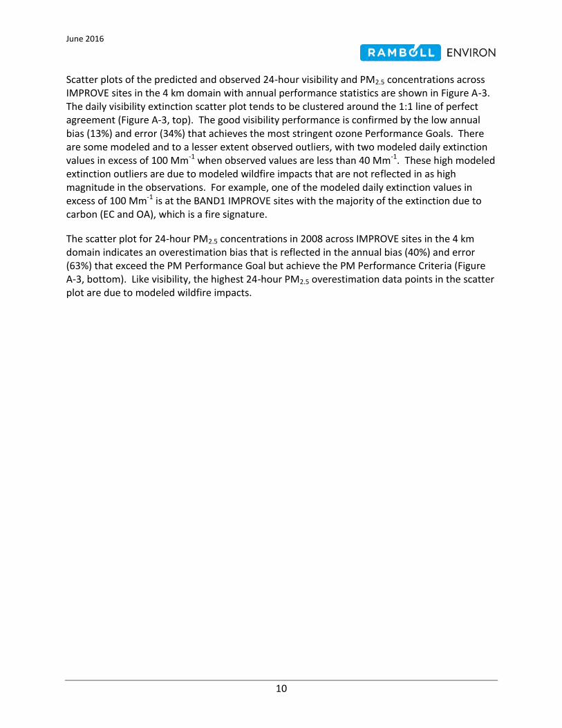
June 2016

10

Scatter plots of the predicted and observed 24-hour visibility and PM2.5 concentrations across IMPROVE sites in the 4 km domain with annual performance statistics are shown in Figure A-3. The daily visibility extinction scatter plot tends to be clustered around the 1:1 line of perfect agreement (Figure A-3, top). The good visibility performance is confirmed by the low annual bias (13%) and error (34%) that achieves the most stringent ozone Performance Goals. There are some modeled and to a lesser extent observed outliers, with two modeled daily extinction values in excess of 100 Mm-1 when observed values are less than 40 Mm-1. These high modeled extinction outliers are due to modeled wildfire impacts that are not reflected in as high magnitude in the observations. For example, one of the modeled daily extinction values in excess of 100 Mm-1 is at the BAND1 IMPROVE sites with the majority of the extinction due to carbon (EC and OA), which is a fire signature.

The scatter plot for 24-hour PM2.5 concentrations in 2008 across IMPROVE sites in the 4 km domain indicates an overestimation bias that is reflected in the annual bias (40%) and error (63%) that exceed the PM Performance Goal but achieve the PM Performance Criteria (Figure A-3, bottom). Like visibility, the highest 24-hour PM2.5 overestimation data points in the scatter plot are due to modeled wildfire impacts.

June 2016

11

Figure A-3. Scatter plots and annual performance statistics of predicted and observed 24-hour visibility extinction (top) and PM2.5 mass concentrations (bottom) for 2008 and all IMPROVE sites in 4 km CGS domain.

June 2016

12

A.4.1.2 Total Visibility Extinction and PM2.5 Mass Performance at Individual Monitoring Sites

Figures A-4 and A-5 displays spatial maps of annual total daily visibility extinction and PM2.5 mass Normalized Mean Bias (NMB) and Normalized Mean Error (NME) performance statistics, respectively, at IMPROVE monitoring sites. Tabular summaries of total extinction and Pm2.5 performance statistics for many metrics (see Table A-2) are provided in Tables A-3 and A-4. The visibility NMB (Figure A-4, top) achieves the ≤±30% PM Performance Goal at all sites but BAND1 (39%), which is also the only site (52%) that the NME just barely doesn’t achieve the error PM Performance Goal (≤50%). CAMx exhibits better visibility performance for the southern two-thirds of the 4 km domain with NMB that achieves the most stringent ozone Performance Goal ≤±15%, whereas the IMPROVE sites in the northern one-third of the 4 km domain have NMB in the 20-39% range.

The CAMx total PM2.5 mass model performance achieves the PM Performance Criteria (≤±60%) at all sites but BAND1 (+124%), albeit with an overestimation bias. Of the 19 IMPROVE sites, only 3 have NMB that fail to achieve the ≤±30% PM Performance Goal with four sites having Fractional Bias that fails to achieve the PM Performance Goal (Table A-4; i.e., 79-84% of the IMPROVE sites have PM2.5 bias that achieves the PM performance goal). The IMPROVE sites where the total PM2.5 mass bias fail to achieve the PM Performance Goal are located in the northern portion of the 4 km domain (i.e., BAND1, SAPE1, MEVE1 and GRCA1). The PM2.5 error performance statistics (NME and FE) achieve the PM Performance Criteria at all sites except BAND1. As seen in the PM2.5 summary statistics in Table A-4, the poor PM2.5 model performance at BAND1 appears to be an outlier with all other sites achieving the PM Performance Criteria for bias and error and most sites bias achieving the PM Performance Goal.

June 2016

13

Figure A-4. Normalized Mean Bias (NMB) of total visibility extinction (top) and total PM2.5 mass (bottom) by IMPROVE site in 4 km domain (PM Goal ≤±30% and PM Criteria ≤±60%).

June 2016

14

Figure A-5. Normalized Mean Error (NME) of total visibility extinction (top) and total PM2.5 mass (bottom) by IMPROVE site in 4 km domain (PM Goal ≤50% and PM Criteria ≤75%).

June 2016

15

Table A-3. Annual total visibility extinction model performance statistics at selected IMPROVE monitoring sites in the 4 km CGS domain and comparison with PM Performance Goals and Criteria (yellow shading indicate PM Performance Criteria is exceeded).

Site N AvObs AvMod MB ME NMB NME FB FE COR

Goal ≤±30% ≤50% ≤±30% ≤50%

Criteria ≤±60% ≤75% ≤±60% ≤75%

BAND1 102 20.8 29.0 8.2 10.8 39.3 51.8 30.5 40.6 0.012

CHIR1 104 22.3 23.3 0.9 5.6 4.1 24.9 6.6 23.7 0.225

GRCA2 97 18.6 22.5 3.9 6.6 20.9 35.7 19.3 31.8 0.069

MEVE1 111 19.3 23.9 4.5 7.5 23.5 38.6 21.1 33.4 0.071

PEFO1 110 21.9 23.1 1.2 6.1 5.4 28.0 7.2 26.4 0.057

SAGU1 93 26.4 28.7 2.3 6.4 8.9 24.4 9.0 23.8 0.187

SAPE1 95 17.4 21.0 3.6 6.1 20.4 35.0 19.3 31.0 0.158

SIAN1 72 23.4 25.0 1.6 6.9 6.9 29.5 5.2 25.7 0.202

SYCA1 111 24.8 24.9 0.1 9.0 0.4 36.2 -0.1 32.8 0.080

June 2016

16

Table A-4. Annual total PM2.5 mass model performance statistics at selected IMPROVE monitoring sites in the 4 km CGS domain and comparison with PM Performance Goals and Criteria (yellow shading indicates PM Performance Criteria not achieved).

Site N AvObs AvMod MB ME NMB NME FB FE COR Goal ≤±30% ≤50% ≤±30% ≤50%

Criteria ≤±60% ≤75% ≤±60% ≤75%

BALD1 118 7.7 7.7 0.0 5.3 -0.6 68.8 11.4 57.1 0.105

BAND1 104 6.8 15.3 8.4 10.2 124.0 149.8 78.6 91.1 -0.238

BOAP1 100 9.1 10.8 1.7 5.8 18.5 64.3 25.0 57.2 0.098

CHIR1 116 8.6 8.7 0.1 4.1 0.9 47.8 14.7 49.2 0.474

GICL1 101 6.0 6.8 0.8 3.6 12.6 59.1 33.1 57.6 0.481

GRCA2 116 5.7 7.9 2.2 4.1 39.4 72.5 42.8 65.2 0.240

IKBA1 122 8.6 8.9 0.3 4.4 2.9 50.5 15.1 48.3 0.318

INGA1 119 10.3 8.3 -2.0 6.2 -19.7 60.3 -3.7 68.7 0.170

MEVE1 115 6.5 8.4 1.8 4.7 28.3 71.8 39.8 64.9 0.423

PEFO1 110 8.5 8.5 0.0 4.7 0.1 56.0 17.1 54.8 0.284

PHOE1 117 26.1 24.0 -2.0 7.9 -7.9 30.4 -6.4 31.6 0.399

QUVA1 109 14.8 11.9 -2.9 6.3 -19.7 42.4 -9.4 43.7 0.283

SAGU1 113 12.2 14.7 2.5 5.6 20.2 45.9 25.1 45.1 0.354

SAPE1 112 5.4 7.7 2.3 3.9 42.9 72.6 50.6 67.5 0.349

SAWE1 109 15.3 11.9 -3.4 6.1 -22.3 40.1 -18.7 43.5 0.255

SHMI1 119 8.4 7.2 -1.2 4.9 -14.6 58.1 5.9 64.1 0.357

SIAN1 77 7.9 8.2 0.3 4.2 4.0 52.9 14.7 51.6 0.330

SYCA1 111 11.7 8.5 -3.2 6.7 -27.3 57.5 -9.2 60.8 0.156

TONT1 116 10.4 10.2 -0.3 4.9 -2.7 46.6 13.2 48.6 0.434

June 2016

17

A.4.2 Evaluation of Visibility and PM2.5 by Species Across the 4 km Domain

Figure A-6 displays soccer plots of monthly performance statistics across IMPROVE sites in the 4 km domain for visibility extinction and PM2.5 concentration for each major PM species. With the exception of the three winter months, the sulfate visibility and mass performance achieves the PM Performance Criteria and even the PM Performance Goals for 5 months and Ozone Performance Goal for August (Figure A-6a, top). For the three winter months, sulfate extinction and concentration has an overestimation bias that makes it fall outside of the range of the PM Performance Criteria.

Nitrate visibility and concentration performance for most months falls between the PM Performance Goals and Criteria with just August and two winter months failing to achieve the Criteria (Figure A6a, middle). There is a general summer underestimation and winter overestimation bias, which is fairly typical of PGM model performance for nitrate. During the summer, the observed and modeled nitrate extinction and concentrations are very low and usually a negligible portion of PM mass or visibility impairment. During the winter, nitrate formation is very episodic and depends on numerous processes and presence of ammonia, whose emissions are highly uncertain. The nitrate performance mostly achieving the PM Performance Criteria represents relatively good PGM model performance for nitrate.

The bottom panels in Figure A-6a display visibility and concentration model performance for Organic Aerosol (OA). With the exception of April, whose error is too large, the remaining 11 months achieve the PM Performance Criteria. The best performing months for OAC occur in the fall and have essentially zero bias with the summer having a slight underestimation and winter a slight overestimation bias. We suspect there may be missing SOA processes in the model that may help explain the summer underestimation bias for OA.

Elemental Carbon (EC) visibility and mass model performance achieves or nearly achieves the PM Performance Criteria, albeit with an overestimation bias for all months (Figure A-6b, top). The overestimation bias is greater for the cooler than warmer months.

The model performance for extinction due to Soil, which is also called other PM2.5 (OPM2.5), is characterized by an over-prediction bias that is at the +60% PM Performance Criteria for Apr-May-Jun and as high as 150% for the winter months, with the rest of the months falling in between (Figure A-6b, middle). There are model-measurement incommensurability with this species with the IMPROVE Soil measurement based on a linear combination of individual elements, whereas the modeled Soil/OPM2.5 species is based on primary PM2.5 emissions that have not been explicitly speciated into other compounds so also includes measurement and speciation artifacts. The model OPM2.5 overestimation of the IMPROVE Soil measurement is common for PGM modeling because of this.

The coarse mass visibility and mass model performance is characterized by a summer underestimation and winter overestimation tendency with 8-9 months achieving the PM Performance Criteria (Figure A-6b, bottom).

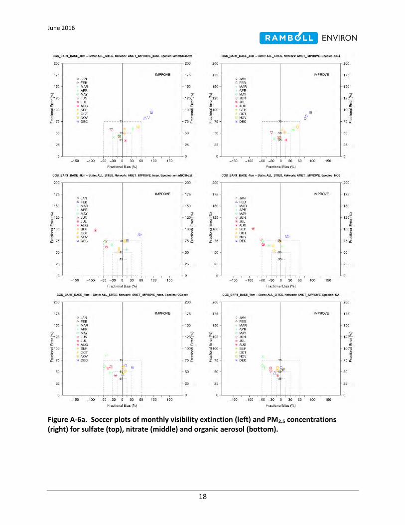
June 2016

18

Figure A-6a. Soccer plots of monthly visibility extinction (left) and PM2.5 concentrations (right) for sulfate (top), nitrate (middle) and organic aerosol (bottom).

June 2016

19

Figure A-6b. Soccer plots of monthly visibility extinction (left) and PM2.5 concentrations (right) for elemental carbon (top), other PM2.5 or Soil (middle) and coarse mass (bottom).

June 2016

20

Figure A-7 displays annual scatter plots of predicted and observed 24-hour extinction (left) and concentrations (right) for six PM component species. Sulfate visibility and mass performance is fairly good with a 20% bias that achieves the PM Performance Goal and an 62-65% error that falls between the PM Performance Goal and Criteria (Figure A-7a, top). The nitrate visibility extinction has a positive 13% overestimation bias but the nitrate concentration performance has a negative -29% underestimation bias (Figure A-7a, bottom). In the nitrate visibility extinction scatter plot there are numerous high overestimation points that are not as prevalent in the nitrate concentrations. This is due to the model’s tendency toward overestimation nitrate in the cooler months and underestimation of nitrate in the warmer months. When averaged over the year, the nitrate concentrations end up having a negative bias. However, when nitrate visibility extinction calculations are made the f(RH) adjustments will tend to inflate the nitrate extinction more in the cooler wetter months than in the warm dry months resulting in an annual nitrate visibility extinction overestimation bias.

The annual OA extinction and concentration performance is shown in the top panels of Figure A-7b. The bias for OA extinction (-9%) and concentration (-21%) both achieve the PM Performance Goal with the error (~60%) falling between the PM Performance Goal and Criteria. The reasons why there is a reduction in the OA underestimation bias when going from concentrations (-21%) to extinction (-9%) is due to the f(RH) effects described above for nitrate and the tendency of the model to underestimate OA in the summer and overestimate in the winter (see Figure A-6a, bottom).

Elemental Caron (EC) extinction and concentrations both exhibit an annual overestimation bias (44% and 37%) and an error (73% and 71%) that falls between the PM Performance Goal and Criteria (Figure A-7b, bottom). As seen in the soccer plots, Soil/OPM2.5 extinction and concentrations are greatly overestimated and fail to achieve the PM Performance Criteria for the reasons described previously (Figure A-7c, top). Finally, coarse mass (CM or PMC) bias for visibility extinction (-3%) and concentration (-24%) achieves the PM Performance Goal but with lots of scatter so that the error (76% and 66%) is at the PM Performance Criteria (Figure A-7c, bottom). Coarse mass has a large contribution from dust whose emissions are more uncertain and has a shorter transport distance so some impacts may be local in nature and subgrid-scale to the model.

June 2016

21

Figure A-7a. Annual scatter plots and performance statistics for 24-hour visibility extinction (left) and PM2.5 mass (right) and sulfate (top) and nitrate (bottom).

June 2016

22

Figure A-7b. Annual scatter plots and performance statistics for 24-hour visibility extinction (left) and PM2.5 mass (right) and organic aerosol (top) and elemental carbon (bottom).

June 2016

23

Figure A-7c. Annual scatter plots and performance statistics for 24-hour visibility extinction (left) and PM2.5 mass (right) and other PM2.5 or SOIL (top) and coarse mass (bottom).

June 2016

24

A.4.3 Site-Specific Evaluation of Visibility by Species

Table A-5 displays annual visibility model performance statistics at IMPROVE monitoring sites by each major component of visibility extinction: AmmSO4, AmmNO3, OA, EC, Soil and Coarse Mass. Annual time series plots of visibility extinction component for each IMPROVE site are given in Figures A-8 through A-16. The visibility performance at each IMPROVE sites by component is discussed in the following sections starting with CHIR1 in the south and going counter clockwise and finishing with BAND1 in the northeast (see Figure A-1). The emphasis of this discussion is on those species of most importance in the CGS BtB modeling, namely AmmSO4 and AmmNO3.

A.4.3.1 Chiricahua (CHIR1)

The annual total visibility extinction model performance statistics at CHIR1 are quite good with low bias (4-7% and error (24-25%) (Table A-3). This is reflected in the time series of predicted and observed total extinction that has low bias, except for one day that is underestimated near the end of September (Figure A-8, top left). The model does slightly overestimate extinction in the winter and slightly underestimate it in the summer. The high observed extinction the end of September is due to AmmSO4 with the AmmSO4 visibility performance at CHIR1 being very good for the rest of the year (Figure A-8, top right) with low bias (-1% and 7%) and error at the PM Performance Goal level (53-54%). The model also predicts the observed extinction due to AmmNO3 quite well for all days except one day in early February that is greatly overestimated (Figure A-8, middle left). The AmmNO3 extinction bias at CHIR1 achieves the PM Performance Goal with the error in between the PM Performance Goal and Criteria.

There is a lot of day-to-day variation in the predicted and observed OA extinction at CHIR1 with the model overall following the seasonal trend in the observations (higher in summer and lower in winter) with bias and error statistics that achieve the PM Performance Goal (Figure A-8, middle right). There is a high observed OA extinction day in mid-April that is not reflected in the model that could be due to fires, the high Soil extinction on this day also supports this hypothesis but the low EC extinction does not. The model tends to overestimate visibility extinction due to EC throughout the year resulting in high bias (65% and 52%) and error (87% and 68%). Extinction due to Soil is also greatly overestimated (> 100%) that is due in part to differences in how the IMPROVE equation and model defines this species (Figure A-8, bottom right). The bias for extinction due to coarse mass (-28% and -19%) achieves the PM Performance Goal with the error (55% and 63%) falling between the PM Performance Goal and Criteria (Table A-5b).

June 2016

25

Table A-5a. Annual model performance statistics for visibility extinction (Mm-1) by species (AmmSO4, AmmNO3 and OA) at IMPROVE monitoring sites in the 4 km CGS domain and comparison with PM Performance Goals and Criteria (bold statistics fail to achieve the PM Performance Criteria).

Site N AvObs AvMod MB ME NMB NME FB FE COR PM Goal ≤±30% ≤50% ≤±30% ≤50%

PM Criteria ≤±60% ≤75% ≤±60% ≤75%

Ammonium Sulfate (AmmSO4) Extinction

BAND1 102 4.5 5.1 0.7 2.8 15.3 62.2 16.3 55.9 0.118

CHIR1 104 5.2 5.1 -0.1 2.8 -1.1 54.6 6.7 53.3 0.242

GRCA2 97 3.7 5.1 1.3 2.9 36.0 76.4 28.3 64.3 0.034

MEVE1 111 4.1 5.6 1.6 2.9 38.2 70.9 30.4 57.4 0.026

PEFO1 110 4.2 5.0 0.8 2.6 18.2 61.4 18.2 55.7 0.091

SAGU1 93 4.8 5.1 0.2 2.8 4.8 57.3 2.4 56.1 0.126

SAPE1 95 3.7 4.8 1.1 2.6 29.4 70.3 27.9 60.2 0.038

SIAN1 72 4.5 5.2 0.7 2.8 15.7 62.8 22.8 57.6 0.171

SYCA1 111 3.9 5.0 1.2 2.8 30.0 72.2 28.4 61.7 0.080

Ammonium Nitrate (AmmNO3) Extinction

BAND1 102 1.3 1.6 0.3 1.3 27.1 99.3 -5.5 69.4 0.327

CHIR1 104 0.6 0.7 0.1 0.5 14.5 73.6 2.4 63.8 0.215

GRCA2 97 0.9 1.0 0.1 0.9 12.5 92.6 -4.3 78.1 0.320

MEVE1 111 1.0 1.9 1.0 1.4 98.0 146.3 16.7 67.9 0.259

PEFO1 110 0.9 1.0 0.0 0.8 3.9 79.2 -27.5 67.2 0.238

SAGU1 93 1.2 0.5 -0.7 0.8 -57.3 67.3 -70.1 82.0 0.154

SAPE1 95 0.9 1.2 0.3 0.8 27.1 86.0 2.7 62.4 0.423

SIAN1 72 1.2 0.7 -0.4 0.8 -37.7 69.0 -40.0 74.7 0.384

SYCA1 111 1.1 1.3 0.2 1.0 18.9 98.7 -15.6 80.3 0.271

Organic Aerosol (OA) Extinction

BAND1 102 1.8 2.0 0.1 1.2 8.1 64.8 -12.8 48.6 0.419

CHIR1 104 1.3 1.1 -0.2 0.6 -15.6 49.0 -12.3 53.9 0.326

GRCA2 97 1.4 1.3 -0.1 0.9 -6.3 68.6 2.1 69.3 0.234

MEVE1 111 1.5 1.2 -0.4 0.9 -23.4 57.5 -14.2 61.1 0.088

PEFO1 110 1.8 1.2 -0.5 0.8 -30.1 42.3 -32.6 50.7 0.506

SAGU1 93 1.9 2.0 0.1 1.1 5.0 55.3 1.0 54.1 0.046

SAPE1 95 1.4 1.0 -0.4 0.7 -27.5 53.3 -29.5 57.2 0.459

SIAN1 72 2.4 2.3 -0.1 1.6 -4.9 66.5 -37.7 63.3 0.578

SYCA1 111 2.4 2.5 0.1 1.8 3.9 74.9 -20.7 59.6 0.254

June 2016

26

Table A-5b. Annual model performance statistics for visibility extinction (Mm-1) by species (EC, Soil and PMC) at selected IMPROVE monitoring sites in the 4 km CGS domain and comparison with PM Performance Goals and Criteria (bold statistics fail to achieve the PM Performance Criteria).

Site N AvObs AvMod MB ME NMB NME FB FE COR PM Goal ≤±30% ≤50% ≤±30% ≤50%

PM Criteria ≤±60% ≤75% ≤±60% ≤75%

Elemental Carbon (EC) Extinction

BAND1 102 1.1 2.0 0.9 1.0 78.7 88.5 45.3 52.9 0.442

CHIR1 104 0.7 1.1 0.4 0.6 65.3 86.5 51.9 67.8 0.230

GRCA2 97 0.8 1.3 0.6 0.8 75.7 103.0 56.8 74.7 0.227

MEVE1 111 0.7 1.1 0.4 0.6 65.8 86.0 47.7 63.8 0.133

PEFO1 110 1.8 1.9 0.0 0.6 1.8 33.0 2.3 33.8 0.533

SAGU1 93 1.4 2.4 1.0 1.2 67.9 83.1 48.6 63.3 0.235

SAPE1 95 0.6 1.0 0.3 0.5 53.1 82.6 43.4 64.3 0.509

SIAN1 72 1.4 2.2 0.7 1.3 52.0 87.9 14.4 53.2 0.320

SYCA1 111 2.1 2.6 0.5 1.4 23.1 66.0 12.0 50.5 0.386

Fine Soil (OPM2.5) Extinction

BAND1 102 1.0 3.7 2.7 2.9 275.3 291.6 126.7 131.6 0.179

CHIR1 104 1.2 2.7 1.6 1.9 133.6 158.6 98.4 106.0 0.449

GRCA2 97 0.9 2.6 1.7 1.8 193.5 209.0 111.9 117.4 0.501

MEVE1 111 0.9 2.7 1.7 1.9 188.2 206.2 113.3 119.2 0.542

PEFO1 110 1.2 2.7 1.5 1.7 126.6 146.1 94.0 100.3 0.486

SAGU1 93 1.8 3.8 1.9 2.2 104.7 119.1 81.1 86.6 0.432

SAPE1 95 1.0 2.7 1.7 1.9 165.5 190.8 112.4 118.5 0.406

SIAN1 72 1.2 2.8 1.6 1.9 136.1 160.2 96.0 103.9 0.378

SYCA1 111 2.2 2.7 0.5 1.9 25.1 85.5 50.9 83.3 0.205

Coarse Mass (PMC) Extinction

BAND1 102 2.1 5.5 3.3 4.2 157.8 198.8 89.7 106.2 -0.293

CHIR1 104 3.2 2.3 -0.9 1.8 -27.8 54.9 -19.3 62.6 0.396

GRCA2 97 1.9 2.1 0.2 1.4 11.2 77.6 12.8 66.9 0.067

MEVE1 111 2.2 2.3 0.1 1.7 4.4 78.6 28.9 72.9 0.440

PEFO1 110 2.8 2.2 -0.7 2.1 -23.8 72.8 -2.6 75.8 0.137

SAGU1 93 4.8 4.8 0.0 2.0 -0.3 41.0 10.0 43.6 0.455

SAPE1 95 1.6 2.1 0.5 1.2 29.6 73.3 44.5 69.4 0.328

SIAN1 72 2.5 1.7 -0.8 1.5 -32.8 58.4 -20.2 67.3 0.213

SYCA1 111 4.1 1.7 -2.4 3.1 -58.3 74.2 -46.1 87.5 0.066

June 2016

27

Figure A-8. Predicted and observe 24-hour average visibility extinction (Mm-1) at Chiricahua (CHIR1) IMPROVE sites for total (top left), AmmSO4 (top right), AmmNO3 (middle left), OA (middle right), EC (bottom left) and SOIL (bottom right).

June 2016

28

A.4.3.2 Saguro (SAGU1)

The total visibility extinction performance at SAGU1 was quite good with bias (9%) and error (24%) that achieves the most stringent ozone Performance Goal (Table A-3). The time series of predicted and observed total extinction at SAGU confirms the performance statistics that the model is unbiased (Figure A-9, top left). Although there are some modeled daily spikes not reflected in the observations, the AmmSO4 extinction performance at SAGU also exhibits very low bias (5% and 2%) but some scatter so the error just barely exceeds the PM Performance Goal (57% and 56%) (Table A-5a and Figure A-9, top right). The observed AmmNO3 at SAGU is generally quite low, with the exception of a large AmmNO3 spike in December (Figure A-9, middle left) . The modeled AmmNO3 at SAGU is also low, and in fact is lower than observed resulting in a large underestimate bias of -57% and -70% (Table A-5a). With the exception of the observed December AmmNO3 extinction spikes, the observations and model agree that visibility impairment due to AmmNO3 at SAGU is small and a negligible part of the extinction budget. The model is also unbiased for extinction due to OA with near zero bias (5% and 1%) and error that just barely exceeds the PM Performance Goal (54-55%) (Table A-5a). This is reflected in the OA extinction time series plots that shows lots of variation in the predicted and observed values, but no systematic bias (Figure A-9, middle right). The usual modeled OA underestimation bias is not seen at SAGU1. As seen at CHIR1, extinction due to EC is overestimated by the model resulting in bias (68% and 49%) and error (83% and 63%) that achieves or barely does not achieve the PM Performance Criteria. Soil extinction is overestimated by the model at SAGU1. Good performance is seem for extinction due to coarse mass at SAGU1 with low bias (0% and 10%) and error (41% and 4%) that achieves the PM Performance Goal (Table A-5b).

A.4.3.3 Sierra Ancha (SIAN1)

The SIAN1 total extinction achieves the PM Performance Goal with low bias (7%b and 5%; Table A-3. The AmmSO4 extinction performance is also good and achieves the PM Performance Goals (Figure A-10, top). Extinction due to AmmNO3 at SIAN has an underestimation bias of approximately -40% but achieves the PM Performance Criteria. The OA extinction performance exhibits a fairly consistent underestimation bias except during modeled daily spikes in March and in the fall. This unusual distribution results in very different bias values using the NME (-5%) and FB (-38%) that still achieve the PM Performance Criteria. The model and observed have fairly good agreement for EC extinction except for a few high modeled days that results in an overestimation bias (52% and 14%). As seen at other sites, Soil extinction is overestimated and extinction due to coarse mass is underestimated but achieves the PM Performance Criteria with some metrics also achieving the PM Performance Goal.

June 2016

29

Figure A-9. Predicted and observe 24-hour average visibility extinction (Mm-1) at Saguro (SAGU1) IMPROVE sites for total (top left), AmmSO4 (top right), AmmNO3 (middle left), OA (middle right), EC (bottom left) and SOIL (bottom right).

June 2016

30

Figure A-10. Predicted and observe 24-hour average visibility extinction (Mm-1) at Sierra Ancha (SIAN1) IMPROVE sites for total (top left), AmmSO4 (top right), AmmNO3 (middle left), OA (middle right), EC (bottom left) and SOIL (bottom right).

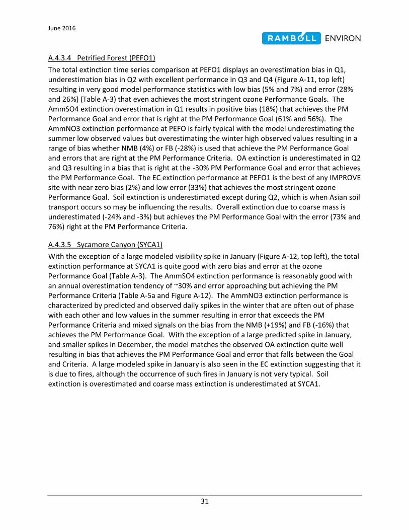
June 2016

31

A.4.3.4 Petrified Forest (PEFO1)

The total extinction time series comparison at PEFO1 displays an overestimation bias in Q1, underestimation bias in Q2 with excellent performance in Q3 and Q4 (Figure A-11, top left) resulting in very good model performance statistics with low bias (5% and 7%) and error (28% and 26%) (Table A-3) that even achieves the most stringent ozone Performance Goals. The AmmSO4 extinction overestimation in Q1 results in positive bias (18%) that achieves the PM Performance Goal and error that is right at the PM Performance Goal (61% and 56%). The AmmNO3 extinction performance at PEFO is fairly typical with the model underestimating the summer low observed values but overestimating the winter high observed values resulting in a range of bias whether NMB (4%) or FB (-28%) is used that achieve the PM Performance Goal and errors that are right at the PM Performance Criteria. OA extinction is underestimated in Q2 and Q3 resulting in a bias that is right at the -30% PM Performance Goal and error that achieves the PM Performance Goal. The EC extinction performance at PEFO1 is the best of any IMPROVE site with near zero bias (2%) and low error (33%) that achieves the most stringent ozone Performance Goal. Soil extinction is underestimated except during Q2, which is when Asian soil transport occurs so may be influencing the results. Overall extinction due to coarse mass is underestimated (-24% and -3%) but achieves the PM Performance Goal with the error (73% and 76%) right at the PM Performance Criteria.

A.4.3.5 Sycamore Canyon (SYCA1)

With the exception of a large modeled visibility spike in January (Figure A-12, top left), the total extinction performance at SYCA1 is quite good with zero bias and error at the ozone Performance Goal (Table A-3). The AmmSO4 extinction performance is reasonably good with an annual overestimation tendency of ~30% and error approaching but achieving the PM Performance Criteria (Table A-5a and Figure A-12). The AmmNO3 extinction performance is characterized by predicted and observed daily spikes in the winter that are often out of phase with each other and low values in the summer resulting in error that exceeds the PM Performance Criteria and mixed signals on the bias from the NMB (+19%) and FB (-16%) that achieves the PM Performance Goal. With the exception of a large predicted spike in January, and smaller spikes in December, the model matches the observed OA extinction quite well resulting in bias that achieves the PM Performance Goal and error that falls between the Goal and Criteria. A large modeled spike in January is also seen in the EC extinction suggesting that it is due to fires, although the occurrence of such fires in January is not very typical. Soil extinction is overestimated and coarse mass extinction is underestimated at SYCA1.

June 2016

32

Figure A-11. Predicted and observe 24-hour average visibility extinction (Mm-1) at Petrified Forest (PEFO1) IMPROVE sites for total (top left), AmmSO4 (top right), AmmNO3 (middle left), OA (middle right), EC (bottom left) and SOIL (bottom right).

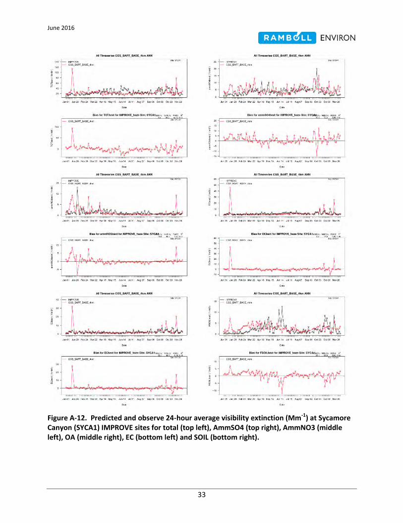
June 2016

33

Figure A-12. Predicted and observe 24-hour average visibility extinction (Mm-1) at Sycamore Canyon (SYCA1) IMPROVE sites for total (top left), AmmSO4 (top right), AmmNO3 (middle left), OA (middle right), EC (bottom left) and SOIL (bottom right).

June 2016

34

A.4.3.6 Grand Canyon (GRCA1)

The annual total extinction performance at GRCA1 achieves the PM Performance Goal but with a 20% overestimation bias (Table A-5a). This annual extinction overestimation is due to overestimations during Q1 (72%) and Q4 (59%) with the performance during Q2 (-1%) and Q3 (15%) being quite good. The GRCA1 Q1 and Q4 total extinction overestimation is from too high extinction due to AmmSO4, AmmNO3 and Soil, as well as EC to a lesser extent (Figure A-13). The AmmSO4 extinction annual performance statistics fall between the PM Performance Goal and Criteria. The extinction due to AmmNO3 performs quite well at GRCA1 with the winter high values and summer low values replicated well resulting in low bias (13% and -4%) but high error (93% and 73%) due to the highly variable daily AmmNO3 extinction spikes during the colder months.

A.4.3.7 Mesa Verde (MEVE1)

Annual total extinction is overestimated at MEVE1 but achieves the PM Performance Goals (Table A-3). This is due to too high total extinction in Q1 and Q4 and is caused by too high AmmSO4, AmmNO3 and Soil extinction (Figure A-16). Better AmmSO4 and AmmNO3 extinction performance is seen during the warmer months, although extinction due to OA is underestimated during the summer. Except for April, when the Asian dust transport is greatest, extinction due to Soil is overestimated the rest of the year.

A.4.3.7 San Pedro Parks (SAPE1)

Total extinction at SAPE1 achieves the PM Performance Goal but with an overestimation bias of ~20% that again is mainly due to AmSO4 and AmmNO3 and Soil overestimation in Q1 and Q4 (Figure A-15). There is a large daily modeled extinction spike in September that is caused mainly from OA and EC so is clearly a modeled wildfire impact that is not reflected in the observations.

A.4.3.8 Bandelier (BAND1)

BAND1 is close to SAPE1 (Figure A-1) so shares many of its performance characteristics but with a larger overestimation bias (39% and 31%; Table A-3). The modeled daily fire impact in September is even greater at BAND1 than at SAPE1 with modeled total extinction exceeding 100 Mm-1. AmmSO4 and AmmNO3 are overestimated with the modeled AmmNO3 overestimation in Q1 being particularly high (Figure A-16).

June 2016

35

Figure A-13. Predicted and observe 24-hour average visibility extinction (Mm-1) at Grand Canyon (GRCA1) IMPROVE sites for total (top left), AmmSO4 (top right), AmmNO3 (middle left), OA (middle right), EC (bottom left) and SOIL (bottom right).

June 2016

36

Figure A-14. Predicted and observe 24-hour average visibility extinction (Mm-1) at Mesa Verde (MEVE1) IMPROVE sites for total (top left), AmmSO4 (top right), AmmNO3 (middle left), OA (middle right), EC (bottom left) and SOIL (bottom right).

June 2016

37

Figure A-15. Predicted and observe 24-hour average visibility extinction (Mm-1) at San Pedro Parks (SAPE1) IMPROVE sites for total (top left), AmmSO4 (top right), AmmNO3 (middle left), OA (middle right), EC (bottom left) and SOIL (bottom right).

June 2016

38

Figure A-16. Predicted and observe 24-hour average visibility extinction (Mm-1) at Bandelier (BAND1) IMPROVE sites for total (top left), AmmSO4 (top right), AmmNO3 (middle left), OA (middle right), EC (bottom left) and SOIL (bottom right).

June 2016

39

A.4.4 Visibility Performance Summary

Figure A-17 displays stacked bar charts of annual total extinction at each IMPROVE sites with the stacked bars showing each component. For most sites, the observed and predicted total extinction are similar, although the modeled value tends to be the same or higher than the observed value. Annual AmmSO4 extinction agrees well at all IMPROVE sites. The annual AmmNO3 extinction also agrees well at most sites, although some have an overestimation (e.g., MEVE1) and others an underestimation (e.g., SAGU1). The largest overestimation site is BAND1 whose overestimation is primarily due to overstated extinction due to Soil and coarse mass.

Stacked extinction bar charts by quarter are shown in Figure A-18. This figure clearly shows that the modeled annual extinction overestimation is primarily due to overstated extinction across several species in Q1 and Q4. The model extinction performance in Q2 and Q3 is quite good.

Figure A-19 displays the stacked bar chart performance for extinction averaged across the best 20 percent (B20%) and worst 20 percent (W20%) days at each IMPROVE site. The model overestimates the average observed extinction on the B20% days, with the overestimation bias approximately a factor of 2 at BAND1 (Figure A-19, top). The B20% days extinction overestimation is mainly due to overstated extinction due to AmmSO4, OA, EC, Soil, coarse mass and sometimes AmmNO3.

The model does a better job at reproducing the observed extinction for the W20% days (Figure A-19, bottom). There is a slight underestimation of the extinction due to AmmSO4 and AmmNO3 with larger underestimation of extinction due to coarse mass at some sites (e.g., SYCA1).

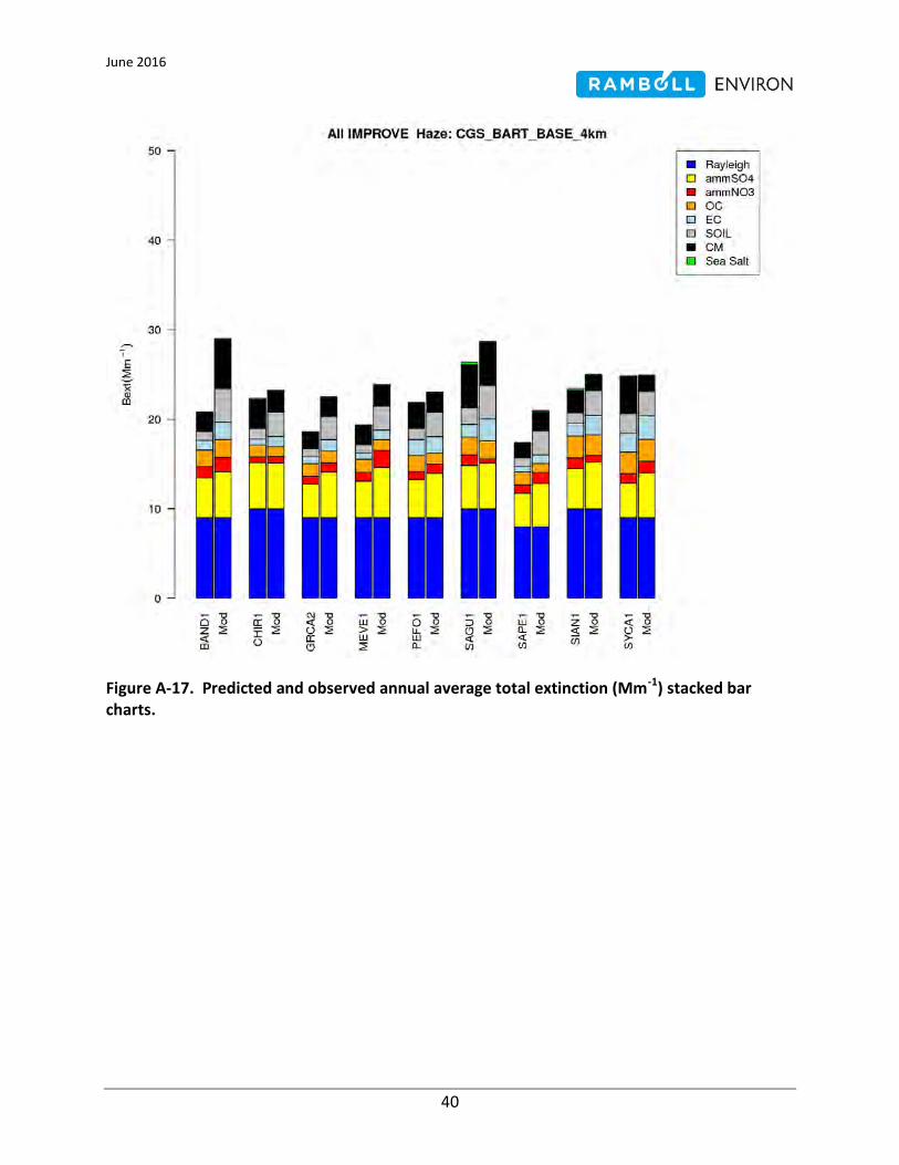
June 2016

40

Figure A-17. Predicted and observed annual average total extinction (Mm-1) stacked bar charts.

June 2016

41

Figure A-18. Predicted and observed seasonal average total extinction (Mm-1) stacked bar charts for Q1 (top left), Q2 (top right), Q3 (bottom left) and Q4 (bottom right)..

June 2016

42

Figure A-19. Predicted and observed extinction for best (top) and worst (bottom) 20 percent days.

June 2016

43

A.5 Model Performance Evaluation Conclusions

The CAMx total visibility extinction achieves the PM Performance Goal on an annual basis as well as for 9 of 12 months with the overestimation bias in the winter months being high enough so that it falls between the PM Performance Goals and Criteria. The visibility performance varies geographically, seasonally and by PM species. The visibility performance at IMPROVE sites in the lower two-thirds of the 4 km CGS modeling domain is quite good meeting the most stringent ozone Performance Goals with the visibility performance at IMPROVE sites in the top third of the 4 km domain having an overestimation bias, but still achieves the PM Performance Goals except at the Bandelier (BAND1) IMPROVE whose overestimation bias is due in part to modeled wildfire impacts that are high enough that the PM Performance Criteria is not achieved.

The seasonal visibility model performance shows good performance for the warmer months and an overestimation bias for the cooler months. The monthly visibility model performance achieves the PM Performance Criteria for all months, the PM Performance Goal for 12 months and the ozone Performance Goal for 7 months, the overestimation bias for the three winter months is sufficiently high that the visibility model performance falls between the PM Performance Goal and Criteria.

The ammonium sulfate (AmmSO4) and ammonium nitrate (AmmNO3) visibility performance is fairly good with 9 of 12 months achieving the PM Performance Criteria. AmmSO4 visibility performance also has many months achieving the PM Performance Goal, but the overestimation bias in the three winter months is sufficiently high that the PM Performance Criteria is not achieved. The seasonal variation of the observed AmmNO3 visibility is reproduced well by the model with extremely low values in the warm months and high values in the cooler months with lots of day-to-day variations. The model does not always match the observed day-to-day variations of high and low AmmNO3 events in the cooler months. Visibility performance due to organic aerosol is also fairly good, albeit with a summer underestimation bias. And visibility performance for elemental carbon and soil exhibits an overestimation bias.

The main objective of the CGS Better-than-BART visibility modeling is to evaluate the trade-offs of visibility benefits between reducing CGS’s NOX versus SO2 emissions. Given that the visibility performance for AmmSO4 and AmmNO3 is fairly good and mostly unbiased with what bias that does occur (slight winter overestimation) being common among AmmSO4 and AmmNO3 and the fact that CAMx incorporates state-of-science sulfate and nitrate formation chemistry algorithms, then the CAMx 2008 12/4 km CGS modeling platform should provide an accurate and reliable database for evaluating the alternative BART modeling scenarios.