Contents lists available at ScienceDirect

Wear

journal homepage: www.elsevier.com/locate/wear

Review of the API RP 14E erosional velocity equation: Origin, applications,misuses, limitations and alternativesF. Madani Sania,⁎, S. Huizingab, K.A. Esaklulc, S. Nesicaa Ohio University, USAb Sytze Corrosion Consultancy, The Netherlandsc Occidental Petroleum Corporation, USA

A R T I C L E I N F O

Keywords:API RP 14EErosional velocityVelocity limitErosionSand erosionErosion-corrosion

A B S T R A C T

Oil and gas companies apply different methods to limit erosion-corrosion of mild steel lines and equipmentduring the production of hydrocarbons from underground geological reservoirs. One of the frequently usedmethods is limiting the flow velocity to a so-called "erosional velocity", below which it is assumed that noerosion-corrosion would occur. Over the last 40 years, the American Petroleum Institute recommended practice14E (API RP 14E) equation has been used by many operators to estimate the erosional velocity. The API RP 14Eequation has become popular because it is simple to apply and requires little in the way of inputs. However, dueto a lack of alternatives and its simplicity, the API RP 14E equation has been frequently misused by it beingapplied to conditions where it is invalid, by simply adjusting the empirical c-factor. Even when used within thespecified conditions and associated applications, the API RP 14E equation has some limitations, such as notproviding any quantitative guidelines for estimating the erosional velocity in the two most common scenariosfound in the field: when solid particles are present in the production fluids and when erosion and corrosion areboth involved. A range of alternatives to the API RP 14E equation that are available in the open literature ispresented. Some of these alternatives overlap with API RP 14E, while others go beyond its narrow applicationrange, particularly when it comes to erosion by solid particles. A comparison between the experimentally ob-tained and calculated erosion by different models is presented. The erosional velocity calculated by some of themodels was compared with that estimated by the API RP 14E equation.

1. Introduction

Erosion of carbon steel piping and equipment is a major challengeduring production of hydrocarbons from underground geological re-servoirs, becoming even more complicated when electrochemical cor-rosion is involved. With the need to maintain production rates, opera-tors continuously drill deeper into such reservoirs and/or use proppantsas well as other fracturing techniques. Thus, deeper aquifers are en-countered, water cuts are increased, more multiphase streams areproduced, and more solids and corrosive species are introduced into theproduction, transportation and processing systems, which in turn leadsto increased erosion and erosion-corrosion problems [1–4].

The terms erosion and erosion-corrosion are often inadequatelydescribed and distinguished. For clarity, erosion is defined as puremechanical removal of the base metal, usually due to impingement bysolid particles, although liquid droplet impingement and bubble

collapse impacts can cause the same type of damage [5–7]. Corrosion isconsidered to be an (electro)chemical mode of material degradation,where metal oxidatively dissolves in a typically aqueous environment.Corrosion can be enhanced by intense turbulent flow; in this case it iscalled flow induced corrosion (FIC) or flow accelerated corrosion (FAC)[8–11]. Erosion-corrosion is a combined chemo-mechanical mode ofattack where both erosion and corrosion are involved [7,12,13]. Theresulting erosion-corrosion rate can be larger than the sum of individualerosion and corrosion rates, due to synergistic effects between erosionand corrosion processes [14–18].

Oil and gas companies have always tried to develop appropriatemethods to limit erosion-corrosion to an acceptable level [1,19,20].One of the commonly used methods is reducing the flow velocity belowa so-called “erosional velocity” limit, where it is thought that no metalloss would occur below this velocity [1,21,22]. However, there havebeen persistent concerns about the validity and accuracy in

https://doi.org/10.1016/j.wear.2019.01.119Received 24 October 2018; Received in revised form 16 January 2019; Accepted 20 January 2019

⁎ Correspondence to: Institute for Corrosion and Multiphase Technology, Department of Chemical and Biomolecular Engineering, Ohio University, 342 W State St.,Athens, OH 45701, USA.

E-mail addresses: fm874012@ohio.edu, fazlollah.madani.sani@gmail.com (F. Madani Sani).

Wear 426–427 (2019) 620–636

0043-1648/ © 2019 Elsevier B.V. All rights reserved.

T

Nomenclature

Normal letters

Ai Empirical constant, Eq. (42)Apipe Cross sectional area of pipe (m2), Eq. (24)At Area exposed to erosion (m2), Eqs. (24), (27)C1 Model geometry factor, Eqs. (25), (27)Cstd r/D of a standard elbow (assumed to be 1.5), Eq. (30)Cunit Unit conversion in Eq. (27) (3.15× 1010), Eqs. (26), (27)D Standard particle diameter (μm), Eq. (36)Deff Effective pipe diameter, Eq. (53)Do Reference pipe diameter (1″ or 25.4mm), Eqs. (28), (40)DP Particle diameter (μm), Eq. (36)E90 A unit of material volume removed per mass of particles at

90° (mm3/kg), Eqs. (35), (36)EL,y Annual surface thickness loss (mm/year), Eq. (27)EL Erosion rate or annual surface thickness loss (mm/year),

Eq. (17)Em Material loss rate (kg/s), Eq. (15)FM Empirical constant that accounts for material hardness,

Eqs. (28), (29)FP Penetration factor for material based on 1″ (25.4mm) pipe

diameter (m/kg), Eqs. (28), (40)Fr/D Penetration factor for elbow radius of curvature, Eqs. (28),

(30)Fs Empirical particle shape coefficient, Eqs. (28), (39)HV Material’s initial Vicker’s hardness (GPa), Eqs. (36), (38),

(41), (43)Ks Fitting erosion constant, Eq. (13)Lo Reference equivalent stagnation length for a 1″ ID pipe

(in), Eqs. (31), (32)QG Volumetric flow rate of gas, Eq. (53)QL Volumetric flow rate of liquid, Eq. (53)Sg Gas specific gravity at standard conditions, (air= 1) Eq.

(2)Sl Liquid specific gravity at standard conditions (water= 1);

use average gravity for hydrocarbon-water mixtures), Eq.(2)Geometry-dependent constant, Eq. (14)

UP Particle impact velocity (m/s) (equal to the mixture fluidvelocity), Eqs. (15), (17), (19), (27)

V Standard particle impact velocity (m/s), Eq. (36)Ve Fluid erosional velocity (ft/s), Eqs. (1), (3), (13)Vf Fluid velocity along the stagnation zone, Eqs. (33), (34),

(50), (51)VL Characteristic particle impact velocity (m/s), Eqs. (28),

(39)Vm Fluid mixture velocity (m/s) (=VSG +VSL), Eq. (14)Vm Mixture velocity, Eq. (46)Vo Fluid bulk (average) velocity (flow stream velocity), Eqs.

(34), (46), (47)VP Particle velocity along the stagnation zone, Eqs. (33), (50)VP Particle impact velocity (m/s), Eq. (36)VSG Superficial gas velocity, Eqs. (44)-(49)VSL Superficial liquid velocity, Eqs. (44)-(49)dP,c Critical particle diameter (m), Eq. (21)dP Particle diameter (m), Eqs. (22), (30)dP Particle diameter, Eqs. (33), (51), (52)mP Mass rate of particles (kg/s), Eqs. (15), (17), (27)n n,1 2 Empirical exponents, Eqs. (37), (38)n n n, ,1 2 3 Empirical exponents, Eq. (43)qs Solid (sand) flow rate (ft3/day), Eq. (13)s q s q, , ,1 1 2 2 Empirical parameters, Eq. (38)uM Mean velocity of two-phase mixture (m/s), Eq. (4)

A Minimum pipe cross-sectional flow area required (in2/1000 barrels liquid per day), Eq. (3)

A Cross-sectional area of the pipe (ft2), Eq. (6)A Dimensionless parameter group, Eqs. (19), (21)B Brinell hardness (B), Eqs. (29), (39), (41)C Empirical constant, Eq. (29)C Empirical constant, Eq. (39)D Pipe internal diameter (mm), Eq. (14)D Inner pipe diameter (m), Eqs. (17), (19), (21), (22), (24)D Pipe diameter (in or mm), Eqs. (28), (40)D Ratio of pipe diameter to 1-in pipe, Eq. (30)D Pipe inner diameter (in), Eqs. (31), (32)E ( ) A unit of material volume removed per mass of particles at

arbitrary angle (mm3/kg), Eq. (35)ER Erosion rate (penetration rate) (mm/y), Eq. (14)ER Erosion ratio (kg/kg), Eqs. (39), (40)F ( ) Impact angle function, Eqs. (39), (42), (43)F ( ) Impact angle function, Eqs. (15), (16), (27)G Correction function for particle diameter, Eqs. (23), (27)GF Geometry factor, Eq. (27)ID Pipe inner diameter, Eq. (53)K High-speed erosion coefficient ( 0.01), Eq. (6)K Material erosion constant ((m/s)-n), Eqs. (15), (27)K , k1, k2, k3 Empirical coefficients, Eq. (36)L Stagnation length (in), Eqs. (31), (32), (34), (52)P Operating pressure (psia), Eqs. (2), (3)P Target material hardness (psi) (= 1.55× 105 psi for steel),

Eq. (6)R Gas/liquid ratio at standard conditions (ft3/barrel) (1

barrel assumed to be 5.61 ft3), Eqs. (2), (3)R Radius of curvature of elbow (Reference of radius of cur-

vature is centerline of pipe), Eq. (18)Re Particle Reynolds number, Eqs. (50), (51)T Operating temperature (°R), Eqs. (2), (3)V Fluid velocity (ft/s), Eq. (5)V Impact velocity of the fluid (ft/s), Eq. (6)-(8)V Velocity to remove the corrosion inhibitor film from the

surface (ft/s), Eqs. (9), (10)V Maximum velocity of gas to avoid noise (m/s), Eq. (11)V Maximum velocity of mixture (m/s), Eq. (12)W Sand flow rate (kg/day), Eq. (14)W Sand production rate (kg/s), Eqs. (28), (40)c Empirical constant (√(lb/(ft s2))), multiply by 1.21 for SI

units, Eq. (1)d Pipe inner diameter (in), Eq. (13)d Sand size (μm), Eq. (14)f Friction factor, Eq. (9)f Maximum value of F ( ), Eq. (43)g Gravitational constant (32.2 ft/s2), Eqs. (6), (9)g ( ) Impact angle function, Eqs. (35), (37)h Erosion rate (mpy), Eq. (6)h Penetration rate (m/s), Eqs. (28), (40)i Empirical exponent, Eq. (42)n Velocity exponent, Eqs. (15), (27)r Elbow radius of curvature (a multiple of D) (e.g. 5D), Eq.

(30)x Particle location along the stagnation zone, Eqs. (33), (34)

Greek letters

c Critical ratio of particle diameter to geometrical diameter,Eqs. (21), (23)

µf Fluid viscosity (pa-s), Eq. (30)µf Fluid dynamic viscosity, Eqs. (33), (51)µG Gas phase dynamic viscosity, Eq. (45)

F. Madani Sani, et al. Wear 426–427 (2019) 620–636

621

determination of this critical velocity, given the complexities of con-joint attack by erosion and corrosion. When the erosional velocity isestimated conservatively (to be too low), the companies inexcusablylose production; when it is determined too optimistically (to be toohigh) then they risk severe damage and loss of system integrity. One ofthe guidelines that has been used extensively over the last 40 years forestimating the erosional velocity is a recommended practice proposedby the American Petroleum Institute called API RP 14E [1,23,24].

API RP 14E was originally developed for sizing of new piping sys-tems on production platforms located offshore that carry single or two-phase flow [25]. Overtime, the application of API RP 14E mostly shiftedto estimation of the erosional velocity, so that it is typically acknowl-edged as the “API RP 14E erosional velocity equation” in the field of oiland gas production.

The widespread use of the API RP 14E erosional velocity equation isa result of it being simple to apply and requiring little in the way ofinputs [26,27]. However, it is often quoted that the API RP 14E ero-sional velocity equation is overly conservative and frequently un-justifiably restricts the production rate or overestimates pipe sizes[28–30]. The present work provides a critical review of literature on theorigin of the API RP 14E erosional velocity equation, its applications,misuses, limitations and finally lists a few alternatives.

2. Summary of API RP 14E

API RP 14E provides “minimum requirements and guidelines for thedesign and installation of new piping systems on production platformslocated offshore”. The API RP 14E offers sizing criteria for piping sys-tems across three flow regimes: single-phase liquid, single-phase gasand two-phase gas/liquid. The API RP 14E sizing criteria for each ca-tegory are briefly discussed below with a focus on how they relate toerosion-corrosion.

(1) Single-phase liquid flow linesThe primary basis for sizing single-phase liquid lines is flow velocityand pressure drop. It is recommended that the pressure should al-ways be above the vapor pressure of liquid at the given tempera-ture, in order to avoid cavitation that could lead to erosion. On theother hand, it is suggested that the velocity should not be less than3 ft/s to minimize deposition of sand and other solids [25]; whichpresumably may lead to underdeposit corrosion attack. No otherlimiting criteria for determining flow velocity are mentioned thatare related to either erosion or erosion-corrosion.

(2) Single-phase gas flow linesFor single-phase gas lines, pressure drop is the primary basis forsizing. Only a passing reference is made to a velocity limitation

related to “stripping a corrosion inhibitor film from the pipe wall”,which clearly points towards erosion-corrosion. However, no spe-cific guidance is offered on how to determine this limitation [25].

(3) Gas/liquid two-phase linesAPI RP 14E lists erosional velocity , minimum velocity, pressure drop,noise, and pressure containment as criteria for sizing gas/liquid two-phase lines. The guideline states that “flow lines, productionmanifolds, process headers and other lines transporting gas and li-quid in two-phase flow should be sized primarily on the basis offlow velocity”, what leads to the erosional velocity criterion. API RP14E recommends that, “when no other specific information as toerosive or corrosive properties of the fluid is available”, the flowvelocity should be limited to the so-called “erosional velocity”,above which “erosion” may occur. API RP 14E suggests the fol-lowing empirical equation for calculating the erosional velocity[25]:

=V ce

m (1)

Even though in the definition of the erosional velocity only erosionis mentioned, the recommended c-factors by the API RP 14E for Eq.(1) cover situations where both corrosion and erosion-corrosion areproblematic. API RP 14E states that “industry experience to dateindicates that for solid-free fluids values of c =100 for continuousservice and c =125 for intermittent service are conservative”, i.e.higher c-factors may be used. Although it is not clearly specified inAPI RP 14E, the solid-free condition mentioned in above statementis meant to cover corrosive fluids (e.g. production water) [31], sothe resulting velocity limit actually refers to situations where FIC/FAC is an issue. “For solid-free fluids where corrosion is not an-ticipated or when corrosion is controlled by inhibition or by em-ploying corrosion resistant alloys”, API RP 14E recommends ahigher c-factor of 150–200 for continuous service and up to 250 forintermittent service [25]. These three scenarios cannot be lumpedtogether; when corrosion is not anticipated only mechanical erosionby liquid droplet impingement can occur, while when inhibition orcorrosion resistant alloys (CRA) are employed erosion-corrosionmight be a problem.API RP 14E further instructs that “if solids production is antici-pated, fluid velocities should be significantly reduced.” However, itdoes not offer any specific guidance, even though this is the mostcritical scenario. Instead, API RP 14E suggests that appropriatec-factors need to be found from “specific application studies”, i.e.through customized testing. Finally, API RP 14E recommends whatseems to be an insurance policy that in conditions under which

µL Liquid phase dynamic viscosity, Eq. (45)µm Viscosity of fluid mixture (kg/m-s), Eq. (19)µm Mixture dynamic viscosity, Eq. (45)

f Fluid density (kg/m3), Eq. (30)f Fluid density, Eqs. (33), (51), (52)G Gas phase density, Eq. (44)L Liquid phase density, Eq. (44)m Gas/liquid mixture density at flowing pressure and tem-

perature (lb/ft3), Eqs. (1), (2)M Mean density of two-phase mixture (kg/m3), Eq. (4)m Fluid mixture density (kg/m3) (= ( +V Vl l g g)/Vm), Eq.

(14)m Density of fluid mixture (kg/m3), Eqs. (19), (20)m The density of mixture (kg/m3), Eq. (12)m Mixture density, Eq. (44)P Density of particle (kg/m3), Eqs. (19), (20)P Particle density, Eqs. (33), (52)

t Density of target material (kg/m3), Eq. (27)c Critical strain to failure (0.1 for steel), Eq. (6)P Total pressure drop along the flow path (psi), Eq. (5)

Gas compressibility factor, Eqs. (2), (3)Dimensionless parameter (mass ratio), Eqs. (50), (52)Particle impact angle (rad), Eqs. (15), (16), (18), (19),(24), (27), (37)Density ratio between particle and fluid, Eqs. (20), (21)Ratio of particle diameter to geometrical diameter, Eqs.(22), (23)Impact angle (rad or degree), Eqs. (39), (42)Impact angle (rad), Eq. (43)Impacting fluid volume rate (ft3/s) (= AV ), Eq. (6)Fluid density (lb/ft3), Eqs. (5) to (10)Density of gas (kg/m3), Eq. (11)Shear strength of the inhibitor interface (psi), Eq. (9)

F. Madani Sani, et al. Wear 426–427 (2019) 620–636

622

solids are present, or corrosion is a concern or c-factors higher than100 for continuous service are used –practically covering all ima-ginable scenarios– periodic surveys are required in order to assesspipe wall thickness [25]. In this statement, a mixture of erosion anderosion-corrosion scenarios is mentioned by API RP 14E, as if theyare indistinguishable. Table 1 summarizes the c-factors suggestedby API RP 14E for different conditions.The API RP 14E erosional velocity equation (Eq. (1)) only needs thegas/liquid mixture density ( m) in terms of input, which makes theequation easy to use. The following empirical equation is suggestedby API RP 14E for calculating m:

=++

S P RS PP RT

12409 2.7198.7m

l g

(2)

After calculating the erosional velocity (Ve), API RP 14E re-commends using the equation below to determine “the minimumcross-sectional area required to avoid fluid erosion”:

=+

AV

9.35 RTP21.25

e (3)

While API RP 14E presents a simple equation to estimate the ero-sional velocity as a sizing criterion for pipework systems carryingtwo-phase gas/liquid flow, it is not clear at all how such a simpleexpression, with only one adjustable constant, can cover a broadarray of scenarios seen in these systems; including various flowregimes (stratified, slug, annular-mist, bubble, churn, etc.), thepresence or absence of solids, the presence or absence of corrosion,with and without inhibition, and mild steel or CRA as the pipematerial. The differences in erosion and erosion-corrosion me-chanisms are so large that it seems next to impossible to capture allthe possible scenarios with one such simple expression. However,before jumping to any conclusion, the origin of this empiricalequation should be examined because it may form a rationale for itsuse.

3. Origin of API RP 14E erosional velocity equation

API RP 14E was first published in 1978. Ever since, its origin hasbeen the subject of much debate in the open literature. The oldest re-ference found proposing an equation similar to the API RP 14E equationis Coulson and Richardson’s Chemical Engineering book from 1979[32]. It suggests the following empirical equation to obtain the velocityat which erosion becomes significant:

=u 15, 000M M2 (4)

By solving Eq. (4) for the velocity (uM) the same expression as theAPI RP 14 equation will be obtained with a c-factor of 122. When ac-counting for the conversion from SI units used in this reference to theImperial units used in the API RP 14 equation, a c-factor of 100 is re-covered. However, there is no information in the book about the originof Eq. (4) either. It can be speculated that Eq. (4) represents some sort of

an energy balance, with the left side representing the kinetic energy ofthe flow and the right side being the amount of energy required to causeerosion. A qualitatively similar argument was presented later by Lotz[33].

In 1983, Salama and Venkatesh [2] speculated that the API RP 14Eequation might be not purely empirical and suggested three possibleapproaches that could theoretically justify its derivation. It is worthsummarizing those arguments in an attempt to bring the reader closerto the origin of the API RP 14E equation:

(1) Bernoulli equation with a constant pressure dropSolving the Bernoulli equation for velocity (V ), assuming no gravityeffects and a final velocity of zero results in Eq. (5), which has asimilar form as the API RP 14E equation.

=V P2(5)

Salama and Venkatesh [2] claimed that a typical total pressure dropfor high capacity wells is between 3000 and 5000 psi. Substitutingthese numbers into Eq. (5) results in a c-factor in the range of77–100. They concluded that although Eq. (5) and the API RP 14Eequation seem to be similar, “they should have no correlation be-cause they represent two completely different phenomena.” [2]Indeed, it is difficult to imagine how the Bernoulli equation can beconnected to erosion of a metal without introducing speculativeassumptions along the way. One such hypothetical scenario wouldbe flow of a fluid through a sudden constriction, such as the dis-charge of a valve or the suction of a pump, which causes an abruptpressure drop that can be estimated by using (5). If the total pres-sure of the system falls below the vapor pressure of the liquid phase,cavitation could happen that leads to metal erosion [34–36]. Si-milar equations to Eq. (5) have been used to estimate the velocitylimit above which cavitation erosion happens in pipeline systems[37–39].

(2) Erosion due to liquid impingementIn another attempt to justify the origin of the API RP 14E equation,Salama and Venkatesh [2] used the following equation introducedby Griffith and Rabinowicz for calculating the erosion rate due toliquid droplet impingement:

=h K VPg

VgP A2

227

12 2

c2

2

(6)

By making a number of arbitrary assumptions, Salama andVenkatesh [2] were apparently able to reduce this equation to aform similar to the API RP 14E equation:

V 300(7)

For more details on the simplification procedure, the reader is re-ferred to the original publication [2]. However, the authors of thispaper determined that it was not possible to reproduce the deri-vation of Eq. (7) and recover the same c-factor (300). It seems thatthere was an inconsistency in the units in the original paper.Craig [40] modified Salama and Venkatesh’s simplifications of Eq.(6) using a high speed coefficient (K ) of 10−5, and units of ft/s forthe penetration rate and psf for the target material hardness (P).Craig [40] proposed that liquid droplet impingement causes da-mage by removing the corrosion product layer from the surface andnot removing the base metal itself as was originally considered bySalama and Venkatesh. Thus, in Eq. (6), Craig substituted the valuesof P and the critical failure strain ( c) for steel with those formagnetite (Fe3O4) (P =1.23×108 psf and c =0.003). Craig’s

Table 1Recommended c-factors by API RP 14E for Eq. (1).

Fluid Recommended c -factor

Continuous service Intermittent service

Solids-free Non-corrosive 150–200 250Corrosive+inhibitor 150–200 250Corrosive+CRA* 150–200 250Corrosive (?) 100 125

With solids Determined from specific application studies

* Corrosion resistant alloy.

F. Madani Sani, et al. Wear 426–427 (2019) 620–636

623

simplification of Eq. (6) with a penetration rate of 10−11 ft/s re-sulted in the following equation:

=V 1503 (8)

The denominators in Eqs. (7) and (8) are different, which proves thepoint made earlier about the inconsistency of units in the Salamaand Venkatesh’ calculations.Using an argument similar to Craig, Smart [41] stated that the APIRP 14E equation represents velocities needed to remove a corrosionproduct layer by “droplet impingement fatigue”, as the flow regimein multiphase systems transits to annular mist flow (presumably anerosion-corrosion scenario). However, Arabnejad et al. [42] showedthat the trend of the erosional velocity calculated by the API RP 14Eequation did not correlate well with empirical data on erosion-corrosion caused by liquid droplet impingement. Deffenbaugh et al.[43] suggested that 400 ft/s is the approximate droplet impinge-ment erosional velocity. The DNV GL recommended practice O501suggests a threshold velocity of 230–262 ft/s to avoid droplet im-pingement erosion in gas-condensate systems [44]. If these velo-cities are plugged into the API RP 14E equation with a c-factorranging from 100 to 300, the resulting mixture density falls be-tween 0.06 and 1.7 lb/ft3, which is extremely low for a gas/liquidtwo-phase flow mixture, making the linkage between the API RP14E equation and liquid impingement implausible. Moreover, ty-pical fluid velocities seen in oil and gas piping applications are farbelow the abovementioned droplet impingement erosional velo-cities, casting doubts that liquid droplet impingement can be con-sidered as a reasonable erosional mechanism behind the API RP 14Eequation [43].

(3) Removal of corrosion inhibitor filmsAs their last attempt, Salama and Venkatesh [2] assumed that theAPI RP 14E equation presents a velocity above which the flow couldremove a protective corrosion inhibitor film from the surface ofsteel tubulars (an erosion-corrosion scenario). According to Salamaand Venkatesh, the resulting erosional velocity can be calculatedfrom the equation below:

=Vgf

8

(9)

Eq. (9) is apparently obtained by setting the flow-induced wallshear stress equal to the shear strength ( ) of the inhibitor film.However, Eq. (9) is not consistent when it comes to the units, i.e.the gravitational constant (g) does not fit into the equation [8,45].Despite this, Salama and Venkatesh [2] derived an equation similarto the API RP 14E equation by simplifying Eq. (9) with equals8000 psi and f equals 0.0015:

=V 35, 000(10)

Craig [40] reported that f =0.0015 is meant for smooth pipes andf =0.03 is more consistent with scale-roughened surfaces. In ad-dition, Craig [40] used psf units instead of psi for in Eq. (9), re-sulting in a constant value of approximately 100,000 instead of35,000 in Eq. (10). Either way, Eq. (10) has the same form as theAPI RP 14E equation; however, the constants found by Salama andVenkatesh as well as Craig were much larger than the c-factorsproposed by API RP 14E, leading to very high velocities –orders ofmagnitude higher than those seen in the oil and gas industry.Therefore, even if the error in Eq. (10) is disregarded, it seems thatthe removal of the corrosion inhibitor film could not have been

used as a background for deriving the API RP 14E equation.In terms of a broader context for this argument, it should be notedthat there is a longstanding belief, which is based on mostly anec-dotal evidence, that above certain fluid velocities corrosion in-hibition fails, what is often attributed to pure mechanical removalof the corrosion inhibitor film by the high wall shear stresses foundin turbulent flow [36,46]. However, recent detailed studies haveshown that pure mechanical removal of the inhibitor film from themetal surface by high-velocity flow is practically impossible, be-cause the shear stresses required to remove a corrosion inhibitorfilm from the surface are of very high order (106–108 Pa), while themaximum wall shear stresses caused by highly turbulent multiphaseflow in oil and gas fields are orders of magnitude lower (ca. 103 Pa)[36,47–49].

At the other end of the spectrum are authors who opined that theAPI RP 14E equation had no theoretical justification and that it is apurely empirical equation. A wide variety of sources was mentioned.For example, Smart [50] stated that the API RP 14E equation was ap-parently obtained from Keeth’s report [51] on erosion-corrosion pro-blems encountered in steam power plants, where multiphase steamcondensate piping systems were used. However, no information onvelocity limitation could be found in this report [31,51,52]. Castle et al.[53] claimed that the API RP 14E equation was formulated based onfield experience with wells in the Gulf Coast area, as a criterion for themaximum velocity in carbon steel piping needed to avoid the removalof protective inhibitor films or corrosion products (an erosion-corrosionscenario). Heidersbach [54] suggested that the API RP 14E equationwas adapted from a petroleum refinery practice in which the flow ve-locity was kept below the API RP 14E erosional velocity to minimizepumping requirements that become prohibitively expensive at highflow velocities. Salama [31] cited Gipson who mentioned that theproposed c-factor in the API RP 14E equation was meant to preventexcessive noise in piping systems. Wood [7] stated that the origin of theAPI RP 14E equation was from US Naval steam pipe specifications.Patton [55] reported that the API RP 14E equation was developed bythe US Navy during World War II with a c-factor of 160 for carbon steelpiping in solid-free fluids. Subsequently, the c-factor was changed to100 when the equation was incorporated by the API. Another anecdoteis that similar equations to the API RP 14E equation with c-factorsranging from 80 to 160 had been used in various oil companies beforethe API committee members wrote the API recommended practice 14E[50]; however, the origin of those equations was not specified.

Clearly, none of the abovementioned theoretical explanations (en-ergy balance, Bernoulli equation, liquid impingement, corrosion in-hibitor/product removal) that supposedly underpin the API RP 14Eequation seem to properly justify its form. The alternative explanationsinvolving anecdotal evidence are even less convincing. Subscribing toany of the above explanations about the origin of the API RP 14E doesnot change the fact that the API RP 14E equation has been used widelyin the oil and gas industry, albeit with varying degrees of success.Therefore, it is worthwhile reviewing some of the publicized applica-tions of the API RP 14E equation, followed by its misuses and limita-tions.

4. Some applications of API RP 14E erosional velocity equation

Although the origin and even the validity of the API RP 14E equa-tion seems to be questionable, its application within the oil and gasindustry has been prevalent. The following are a few examples of theapplication of the API RP 14E equation in the oil and gas industry.

Deffenbaugh and Buckingham [43] reported that Atlantic RichfieldCompany (ARCO) considered the API RP 14E equation as overly con-servative for straight tubing with non-corrosive solid-free fluids. ARCOrecommended a c-factor of 150 for continuous service and a c-factor of250 for intermittent service when corrosion is prevented or controlled

F. Madani Sani, et al. Wear 426–427 (2019) 620–636

624

by dehydrating the fluids, applying corrosion inhibitors or employingCRAs [43]. It is not entirely clear in this scenario how metal loss hap-pened at all, when there were no solids in the flow stream, neither wasthere any corrosion.

Salama [24] has quoted Erichsen who reported data from a con-densate field in the North Sea operating with a c-factor of 726(equivalent to a flow velocity of 286 ft/s) for 3 years until a failureoccurred in AISI 4140 carbon steel tubing at the flow coupling, whichwas attributed to liquid droplet impingement. Another operator in theNorth Sea chose a c-factor of 300 as the upper limit for the Gullfaks oilfield subsea water injectors completed with API L80 13Cr tubing.

Chevron produced from a gas-condensate reservoir in the NorthWest Shelf of Western Australia with a pressure of 4500 psi and tem-perature of 110 °C at a velocity just below the wellhead of 121 ft/s(corresponding to a c-factor of 400) in 7″ OD tubing and at 59 ft/s(corresponding to a c-factor of 200) in 9 5/8″ OD tubing with no failure[56].

At North Rankin offshore gas field in the North West region ofWestern Australia, velocities up to 98 ft/s, three times the API re-commended erosional velocity, were handled in carbon steel tubingover long periods of production without any sign of erosion [53].

In a field study done by the National Iranian Oil Company on fourgas wells in the Parsian gas-condensate field in southern Iran, c-factorsin the range of 149 (velocity of 55 ft/s) to 195 (velocity of 74 ft/s)caused no unexpected erosion damage. Therefore, the operator sug-gested using an average c-factor of 170 as a safe value for all those wells[27]. In similar research conducted on four gas-condensate wells in theSouth Pars gas field in southern Iran, it was reported that c-factors inthe range of 138–193 were safe for production [57].

BP Amoco limited the velocities in production from gas wells in theEndicott field of the Alaskan North Slope to approximately three timesthe API erosional velocity based on an experience that fluids with verysmall amounts of entrained solids flowing through SS pipelines causedminimal risk of erosion at those velocities [58].

Before 1993, Shell used a modified version of the API RP 14Eequation with a c-factor of 160 for sand-free, 120 for moderate-sandand 80 for severe-sand service. Since 1993 and before switching to amodified version of the Tulsa Model (see Section 7.5), Shell stoppedusing the API RP 14E equation and set the limiting erosional velocitydirectly according to the type of failure mechanism, and verified thatvelocity with appropriate monitoring and inspection [59].

TOTAL has been using the API RP 14E equation to define erosion-corrosion velocity limits for carbon steel facilities, sometimes in com-bination with fixed velocities not to be exceeded, whichever is smaller.For CRAs, copper alloys, and nonmetallic materials fixed velocity limitsare solely used. TOTAL has specific criteria (decision tables) in case oferosion-corrosion for determining the most appropriate c-factor rangingfrom 75 to 250 based on the concentration of solid particles, the mainproduced phases (liquid or multiphase, gas dominant or oil dominant),the corrosiveness of the water (if any), and the presence of corrosioninhibitors. Below is a summary of the decision tables:

• c-factors< 100 for corrosive fluids containing significant amountsof solid particles, which are considered highly detrimental in termsof erosion-corrosion;• c-factors from 100 to 160 for various liquid or multiphase fluids,depending on their corrosiveness and the confidence given to thecorrosion mitigation;• c-factors from 200 to 300 for fluids not significantly corrosive andwithout significant amount of solid particles (e.g. deaerated sea-water, dry gas, etc.) [60].

TOTAL apparently does not use the API RP 14E equation to de-termine the erosional velocity when pure mechanical erosion is in-volved. TOTAL defines an indicative velocity limit of 50m/s for pas-sivating alloys such as stainless steel (SS) as a typical “hold point”

above which pure erosion might happen in the presence of traceamounts of solid particles. This 50m/s value is not a definitive velocitylimit but rather a break point for further assessment of the conditions.Generally, TOTAL uses specially developed erosion models such as theDNV GL model (Section 7.4) or the Tulsa model (Section 7.5) for pre-dicting pure erosional damages [60].

It is quite possible that the above practices no longer reflect thecurrent practices being used in the mentioned companies. Even then, inalmost all the reported field cases, c-factors higher than those suggestedby API RP 14E were used, with a very large spread.

5. Misuses of API RP 14E erosional velocity equation

The API RP 14E equation was intended for establishing an erosionalvelocity in “new piping systems on production platforms located off-shore”, transporting gas and liquid two-phase fluids. API RP 14E clearlystates a specific range of c-factors for “solid-free fluids where corrosionis not anticipated or when corrosion is controlled by inhibition or byemploying CRAs”. These conditions are commonly recognized as“clean” service. Presumably, for solid-free corrosive fluids the API RP14E equation can also be used with a c-factor of 100, although it isconsidered conservative. In the presence of solids, reduced c-factors arerecommended if “specific application studies have shown them to beappropriate”, without an explicit guideline provided by the API RP 14E[25]. Obviously, in conditions other than those mentioned above, theAPI RP 14E equation should not be used, at least not without a properjustification.

Probably due to a lack of alternatives and its simplicity, the API RP14E equation has been used widely with arbitrary choice of c-factors fora variety of unfitting conditions such as single-phase flow service anduninhibited corrosive systems with a corrosion product layer[24,52,61]. Another problematic use of the API RP 14E equation wasfor sizing downhole tubulars, which were not included in the originalrecommended practice [23,50,54]. The steel grade recommended fordownhole tubulars (specified in API SPEC 5CT [62]) is generallystronger and harder than API 5 L steel grade recommended in API RP14E [54]. Therefore, if applicable at all, the original API RP 14E ero-sional velocity would be conservative for downhole tubulars.

The lack of generality of the API RP 14E equation was clearly re-cognized in the past, and some attempts were made to improve itsperformance by presenting functions for calculation of the c-factor atdifferent operating conditions [31]. However, this just compounded theproblem where an empirical equation–which already performed in-adequately and could not be extrapolated across different conditions–was altered by making it even more complex, without proper justifi-cations.

In the most general sense, the misuse of the API RP 14E equationstems from its doubtful origin and unclear theoretical basis, what led toit being used in all kinds of conditions and applications for which it wasnot intended. This is based on a problematic assumption (often implicit)that the API RP 14E equation can be used as a means of generalizingobserved empirical erosion, FIC/FAC or erosion-corrosion data to de-rive safe operational velocities for a broad variety of conditions, usuallyoutside operational or experimental ranges. This assumption ignoresthe fact that the mechanism and the rate of degradation can be verydifferent (by orders of magnitude) depending on type of service or evenwithin the same type of service. Therefore, the API RP 14E equationcannot be simply applied to all kinds of conditions by just modifying thec-factor, assuming that the equation is universally valid and it will givereasonable values.

The dubious origin and the unfavorable assessment of the validity ofthe API RP 14E equation cannot be ignored, boldly assuming that it iscorrect and can be used unquestionably (obviously done so many timesbefore); one should be aware of its serious limitations, which aresummarized in the following section.

F. Madani Sani, et al. Wear 426–427 (2019) 620–636

625

6. Limitations of API RP 14E erosional velocity equation

The API RP 14E equation while offering a simple approach to cal-culate the erosional velocity, has some serious limitations:

• The equation only considers the density of fluid in calculating theerosional velocity, while many other influential factors such as pipematerial, fluid properties, flow geometry and flow regime are notaccounted [23,63,64].• The API RP 14E equation treats flow lines, production manifolds,process headers and other lines transporting oil and gas similarly interms of limiting the velocity. However, areas with flow dis-turbances such as chokes, elbows, long radius bends, and tees,where most of the erosion/corrosion problems occur, are not dif-ferentiated by the API RP 14E equation [63,65].• The API RP 14E equation suggests that the limiting erosional velo-city increases when the fluid density decreases. This does not agreewith experimental observations for sand erosion and liquid dropletimpingement in which erosion is higher in low-density fluids [2,23].In high-density fluids most solid particles are carried in the center ofthe flow stream without significantly impacting the surface [2].Moreover, the presence of a high-density fluid cushions the impactof solid particles or droplets at the pipe wall. Thus, a higher limitingerosional velocity can actually be applied to fluids with a higherdensity [21].• The API RP 14E equation does not offer any guidelines regardinghow to estimate the erosion rate, neither below nor above the lim-iting erosional velocity. It also does not specify a general allowableerosion rate, in terms of rate of wall thickness loss (e.g. 5–10mpy)[23].• Probably the most significant limitation of the API RP 14E equationis that it does not provide any quantitative guidelines for estimatingthe erosional velocity when solids are present in the production fluid(erosion) or when erosion and corrosion are both an issue (erosion-corrosion), assuming that c =100 is defined for corrosion service.Some amount of solid particles as well as a certain degree of cor-rosion are almost inevitable in real production systems [43,50].Even in so-called “sand-free” or “clean” service, where sand pro-duction rates are as low as a few lb/day, erosion and erosion-cor-rosion damage could be very severe at high production velocities[23]. Therefore, in most of the alternatives to the API RP 14Eequation (described below), the effect of erosion by sand particles isthe focus. However, the effects of flow on mixed erosion-corrosionscenarios have not been properly addressed in the open literaturedue to the complexity of erosion-corrosion process. Over the pastdecade an approach called erosion-corrosion mapping sometimes incombination with computational fluid dynamics (CFD) has beenemployed in modeling of erosion-corrosion [66]. Erosion-corrosionmapping identifies the relative contributions of erosion, corrosion(whether it is active dissolution or passivation), flow and their sy-nergistic effects on the total wastage rate [67]. For review of recentadvances in the area of predictive models for erosion-corrosion, thereader is directed to Refs. [66–68].

7. Alternatives to API RP 14E erosional velocity equation

Given the problematic origin of the API RP 14E erosional velocityequation, its misuses and limitations, it is worthwhile to take a look atsome key alternatives that are available in the open literature.

When it comes to the intent and scope, some of these alternativesdiscussed below overlap largely with API RP 14E, and in some aspectsgo beyond the narrow application range of the API RP 14E erosionalvelocity equation. Examples are the NORSOK P-002 standard [68] andto some extent the recommendations of Svedeman and Arnold [63].

In other cases, the alternatives focus on addressing one of the mostimportant limitations of the API RP 14E equation –how to derive

velocity limits in the presence of solid particles, beyond just arbitrarilyusing the API RP 14E erosional velocity equation with a smallerc-factor. These alternatives are usually based on field experience, em-pirical correlations or theoretical models. Most theoretical modelsevaluate erosion based on the displaced volume of metal or dissipationof energy during particle impact on the metal surface [69]. The best-known examples of such sand erosion models that have been commonlyused in the oil and gas industry are the Salama model, the DNV GLmodel and the various versions of the Tulsa model. In the followingsections, these alternatives are reviewed and compared with each other,whenever possible.

7.1. NORSOK P-002 standard

The NORSOK P-002 standard [68] was developed by the Norwegianpetroleum industry to provide “requirements for the following aspectsof topside process piping and equipment design on offshore productionfacilities: design pressure and temperature; safety instrumented sec-ondary pressure protection systems; line sizing; system and equipmentisolation; and insulation and heat tracing.” NORSOK P-002 definesstandard criteria for sizing pipes in new installations, mainly based onpressure drop and erosional velocity, similarly as is done in API RP 14E.Actually, the NORSOK P-002 standard recommends that sizing lines ingeneral should be in accordance with ISO 13703 [70], which is basedon API RP 14E. Just like API RP 14E, the NORSOK P-002 standard di-vides the flow lines into three main categories: single-phase gas, single-phase liquid and two-phase/multiphase gas/liquid lines [68]. Theerosional velocity limits for each category are briefly discussed below:

1. Single-phase gas linesFor single-phase gas lines where pressure drop is not critical, thestandard requires not to exceed velocities, which may create noiseor vibration problems. As a rule-of-thumb, the standard suggestskeeping the velocity below the following equation or 60m/s,whichever is lower, to avoid noise problem:

= ×V 175 (1/ )0.43 (11)

The constant 175 may be replaced with 200 during process upsets, ifthe noise level is acceptable. Although Eq. (11) is for avoiding noise,it is similar in form to the API RP 14E equation. The standard statesthat if solid particles exist in the gas, particle erosion and an al-lowable erosion rate should be considered for determination of themaximum velocity, without being any more specific about it [68].

2. Single-phase liquid linesFor single-phase liquid lines, the standard advises to keep the ve-locity sufficiently low to prevent problems with erosion, water-hammer pressure surges, noise, vibration, and reaction forces.Table 2 summarizes the recommended maximum velocities for dif-ferent conditions and materials in continuous service, although isnot clear how these limits were derived and what was the limitingCriterion. For intermittent service, the NORSOK P-002 standard al-lows using a maximum velocity of 10m/s depending on the dura-tion and frequency of operation [68].

3. Two-phase and multiphase gas/liquid linesThe NORSOK P-002 standard states that: “Wellhead flow-lines,production manifolds, process headers and other lines made of steeland transporting two-phase or multiphase flow, have a velocitylimitation. When determining the maximum allowable velocity,factors such as piping geometry, well-stream composition, sandparticle (or proppant) contamination and the material choice for theline shall be considered.” Then the standard recommends the fol-lowing equation to calculate the maximum velocity:

= ×V 183 (1/ )m0.5 (12)

F. Madani Sani, et al. Wear 426–427 (2019) 620–636

626

NORSOK P-002 does neither indicate the source nor the reasoningbehind Eq. (12), even if it is obvious that in form it is identical to theAPI RP 14E erosional velocity equation. When adjusting for the units,the constant in Eq. (12) matches with the c-factor of 150 recommendedby API RP 14E.

For non-corrosive well streams and for corrosion resistant pipematerials, with small amounts of solid particles (typically less than30mg sand/liter in the mixed flow) the NORSOK P-002 standard limitsthe maximum velocity to 25m/s. For well streams with larger amountsof solids, the NORSOK P-002 standard suggests calculating the max-imum allowable velocity based on “sand concentration, piping geo-metry (bend radius, restrictions), pipe size, and added erosion allow-ance.” For this, one presumably needs to use erosion models such asthose described below; however, no more specific guidance is provided[68].

For corrosive service (apparently in case of FIC/FAC and erosion-corrosion) where carbon steel piping is used, the NORSOK P-002standard recommends restricting the maximum velocity to 10m/s toavoid removal of the protective corrosion product layer and/or corro-sion inhibitor films, although the rationale behind this limiting velocityis not mentioned [68].

Comparing the velocity limits given by the NORSOK P-002 standardwith those estimated by the API RP 14E equation at similar conditionsshows that the NORSOK P-002 standard is less conservative than theAPI RP 14E equation.

7.2. Svedeman and Arnold

Svedeman and Arnold [63] recommended using the following cri-teria for determining the erosional velocity in “flow lines, productionmanifolds, process headers, and other lines transporting gas and liquidtwo-phase flow”:

(1) For clean serviceClean service was defined as sand-free non-corrosive fluids (absenceof corrosive species or application of corrosion resistant alloys orcorrosion inhibitors), where liquid-droplet impingement is the onlypossible cause of erosion of the base metal. Based on various la-boratory studies, Svedeman and Arnold suggested that no erosionoccurs up to at least 100 ft/s (possibly even up to 300 ft/s) for theclean service.

(2) For erosive serviceFor erosive service involving solid particles, Svedeman and Arnold[63] adopted the following equation for predicting the erosionalvelocity in pipe fittings based on Bourgoyne’s empirical approach

[72]:

=V K dqe s

s (13)

Eq. (13) was derived based on an allowable metal erosion rate of 5mpy. The values of the fitting erosion constant (Ks) for differentcomponent geometries, materials and flow regimes can be found inRef. [73].

(3) For corrosive serviceAccording to Svedeman and Arnold, in corrosive service, the ero-sion criterion is removal of the corrosion product layer from thesurface due to liquid droplet impingement, which occurs when theflow regime is annular-mist. Therefore, the velocity should be keptbelow the transition velocity for the annular-mist flow regime.However, it is mentioned that further experimental work is neededto prove the appropriateness of this approach.

(4) For erosive-corrosive serviceFor erosive-corrosive service, the mechanism of material loss is thecombined effect of erosion and corrosion. No velocity limit is pro-posed in this case because the interaction of erosion and corrosionis complicated. This case was left open for further investigations[63].

7.3. Salama model

Salama [24] proposed the following criteria for estimating theerosional velocity in multiphase flow:

(1) For solid-free, non-corrosive fluids when pressure drop is not aconcern, the API RP 14E equation with a c-factor of 400 is re-commended (apparently covering liquid droplet impingement).

(2) For solid-free, corrosive fluids, the API RP 14E equation withc-factors higher than 300 can be used, provided that the inhibitorsbeing used in the system remain effective at velocities corre-sponding to these c-factors (clearly referring to an FIC/FAC sce-nario).

(3) For sand-laden fluids, the erosional velocity can be calculated fromEq. (14) by considering an allowable erosion rate for the system, forexample 0.1 mm/y.

=ERS

WV dD

1m

m2

2m (14)

Eq. (14) is a semi-empirical equation for predicting erosion causedby sand-laden multiphase fluids in pipe bends [24]. Salama sug-gested a value of 5.5 for the geometry-dependent constant S( )m forpipe bends based on experimental results. The effect of bend radiuswas not considered in the Salama model because test results did notshow a major difference in the erosion rates for 1.5 and 5D bends[24].

7.4. DNV GL-RP-O501

DNV GL-RP-O501 is a guideline on “how to safely and cost effec-tively manage the consequences of sand produced from the oil and gasreservoirs through production wells, flowlines and processing facil-ities.” [44] Major oil and gas operators such as Statoil, Norsk Hydro,ConocoPhillips, and Amoco have contributed to the development of thisguideline [74]. DNV GL-RP-O501 qualitatively ranks the erosion po-tential for piping systems with reference to bulk flow velocities, con-sidering the flow velocity as the only parameter that affects erosion(Table 2-1 of the original standard). DNV GL-RP-O501 suggests thefollowing general empirical equation for quantitative assessment ofsand particle erosion [44]:

=E K U F m( )nm P p (15)

Table 2Recommended maximum velocities for liquid lines according to NORSOK P-002[68].

Fluid Maximum velocity (m/s)

CS SS/Titanium CuNic GRP

Liquids 6 7b 3 6Liquids with sandd 5 7 n/a 6Liquids with large quantities of mud or siltd 4 4 n/a n/aUntreated seawatera 3 7 3 6Deoxygenated seawater 6 7b 3 6

CS: carbon steel; SS: stainless steel; GRP: glass fiber-reinforced plastic.a For pipe diameters less than 8 in (DN 200), BS MA-18 standard [71] issuggested.

b For SS and titanium the maximum velocity is limited by system design(available pressure drop/reaction forces). 7 m/s may be used as a typicalstarting value for sizing.

c Minimum velocity for CuNi is 1m/s.d Minimum velocity for liquids with sand should be in accordance with ISO13703 [70].

F. Madani Sani, et al. Wear 426–427 (2019) 620–636

627

For CS, duplex SS, 316 SS, and Inconel (Ni-Cr alloy), the materialcoefficients K( ) and the velocity exponent (n) are 2×10−9 and 2.6,respectively. For other materials, the reader is referred to Table 3-1 ofthe original standard. The particle impact velocity (UP) is assumed to beequal to the mixture flow velocity (V )m , which is the summation ofsuperficial velocities of all phases. The impact angle function (F ( ))describes the dependency of erosion on the particle impact angle. Forductile materials including steel grades, F ( ) can be calculated fromthe following equation [44]:

= +F sin

F

( ) 0.6[ sin ( ) 7.2( sin ( ) ( ))] [1 exp( 20 )]

( ) [0, 1] for 0,2

2 0.6

(16)

Eq. (15) is the general correlation for erosion rate prediction de-veloped empirically by Finnie in 1960 [75]. DNV GL-RP-O501 suggestscorrections to Eq. (15) for different piping components (e.g. straightpipes, elbows, blinded tees, welded joints, and reducers), accounting forparameters such as size, concentration, and multiple impact of sandparticles; the geometry of components; and the distance of straightpiping between the components. These corrections were determined bydetailed CFD erosion simulations and by comparison of model resultswith field experience [44].

For smooth and straight pipes under turbulent conditions, the sug-gested equation is as follows:

= ×E U m D2.5 10L5

P2.6

p2 (17)

It should be noted that Eq. (17) is independent of the fluid density,viscosity, and particle size.

For disturbed flow geometries, different procedures are suggested tocalculate the erosion rate. As an example, below is the procedure forpredicting the erosion rate in bends [44]:

(1) Calculate the characteristic impact angle ( ):

=R

arctan 12 (18)

For a 5D bend, R and are equal to 5 and 0.3, respectively.(2) Compute the dimensionless parameters A and :

=AU D

µtan ( )m

2P

P m (19)

= P

m (20)

(3) Calculate the ratio ( ) and the critical ratio ( c) of particle diameter(dP) to geometrical diameter (D) using the parameters obtained instep 2:

= =< <d

D 0 or

0 0.1

0.1 0. 1cA

c

P,c1

[1.88 ln( ) 6.04] c

c (21)

= dD

P(22)

(4) Determine the particle-size correction function (G) by using theparameters found in step 3:

=<

G1

c

c

c

(23)

(5) Calculate the characteristic pipe bend area exposed to erosion:

= =A D A4sin ( ) sin ( )t

2 pipe

(24)

(6) Determine the value of the impact angle function from Eq. (16) byusing the angle found in Step 1.

(7) The model/geometry factor (C1) is set equal to:

=C 2.51 (25)

C1 accounts for multiple impact of the sand particles, concentrationof particles at the outer part of the bend and model uncertainty.

(8) For m/s to mm/y conversion, the following unit conversion factormust be used:

= = ×C 1000 3600 24 365 3.15 10unit10 (26)

(9) The maximum erosion rate (mm/y) in a pipe bend is estimated byusing the following expression:

=E K F UA

G C GF m C( ). n

L,yP

t t1 P unit

(27)

The geometry factor (GF) is considered to be 1 based on an as-sumption that the straight pipe section upstream the bend is greaterthan 10D. When the distance of straight piping is less than 10D, a dif-ferent GF should be used. For more details about GF and other type offlow geometries, the reader is referred to the original standard.DNV GL-RP-O501 suggests that for each specific system design andoperating conditions, further CFD erosion simulations and/or experi-mental investigations might be needed to estimate the erosion rateaccurately [44].

For an allowable erosion rate (e.g. 0.1 mm/y), the erosional velocitycan be calculated by solving Eq. (27) for UP. The empirical modelssuggested by DNVGL-RP-O501 only address erosion by solids and donot account for erosion-corrosion, or other mechanisms such as dropletimpingement erosion or cavitation. The models are applicable onlywhere quartz sand is the erosive agent. Moreover, there are limitationsto the range of model input parameters, found in Table 4-1 of the ori-ginal standard [44]. The DNV GL model is applicable to all multiphaseflow regimes [76]. An engineering software called Pipeng Toolbox(pipeng.com) has been developed based on DNV GL-RP-O501 that en-ables a simple and time efficient assessment of sand erosion potentialfor standard piping components.

7.5. Tulsa model

The Tulsa model refers to a series of semi-empirical models devel-oped by the Erosion/Corrosion Research Center (E/CRC) at TheUniversity of Tulsa for estimating erosion rate and safe operating ve-locity in oil and gas flow lines where sand is present [77,78]. The Tulsamodel is currently the most widely used tool for sand erosion assess-ment in major oil and gas companies. The original model was devel-oped in 1993 for single-phase flow; however, over time it was extendedto cover multiphase flow conditions [23,79,80]. Eq. (28) is one of theearly versions of the Tulsa model that allows the calculation of themaximum erosion rate in elbows for both single and multiphase flow[80]:

=( )

h F F F F W VD

D

M s P r/D 2 L1.73

o (28)

The pipe diameter (D) and the sand production rate (W ) are as-sumed to be known. The material hardness coefficient (FM) that ac-counts for the effect of target (pipe) material on erosion is obtained

F. Madani Sani, et al. Wear 426–427 (2019) 620–636

628

using the following equation [77]:

=F C BM0.59 (29)

Table 3 lists the values of Brinell hardness (B) and empirical con-stant (C) for different pipe materials.

The particle shape coefficient (Fs) is an empirical parameter used toaccount for the effect of particle shape on erosion. Table 4 shows thevalues of Fs for different particle shapes.

The penetration factor (FP) was defined as the decrease in thethickness of the eroded material per unit of mass loss of that samematerial. It can be seen as a measure of how concentrated the erosionattack is, depending on the geometry of the component. FP was estab-lished for a reference pipe with 1-in ID (Do =1 in). The term D D( / )o

2 inEq. (28) was used to correct Fp for the pipe diameter [79]. Table 5shows the Fp values for different geometries.

The penetration factor for elbow radius (Fr/D) is a semi-empiricalparameter developed to take into account the effect of elbow geometryand particle size on erosion. The following equation was suggested tocalculate Fr/D for a particle density of approximately 165 lb/ft3

(2650 kg/m3) [80]:

= + +Fµ

drD

Cexp 0.1 0.015 0.12r/Df0.4

f0.65

p0.3 f

0.25std

(30)

For pipe geometries other than the elbow, Fr/D was presumably con-sidered to be 1.

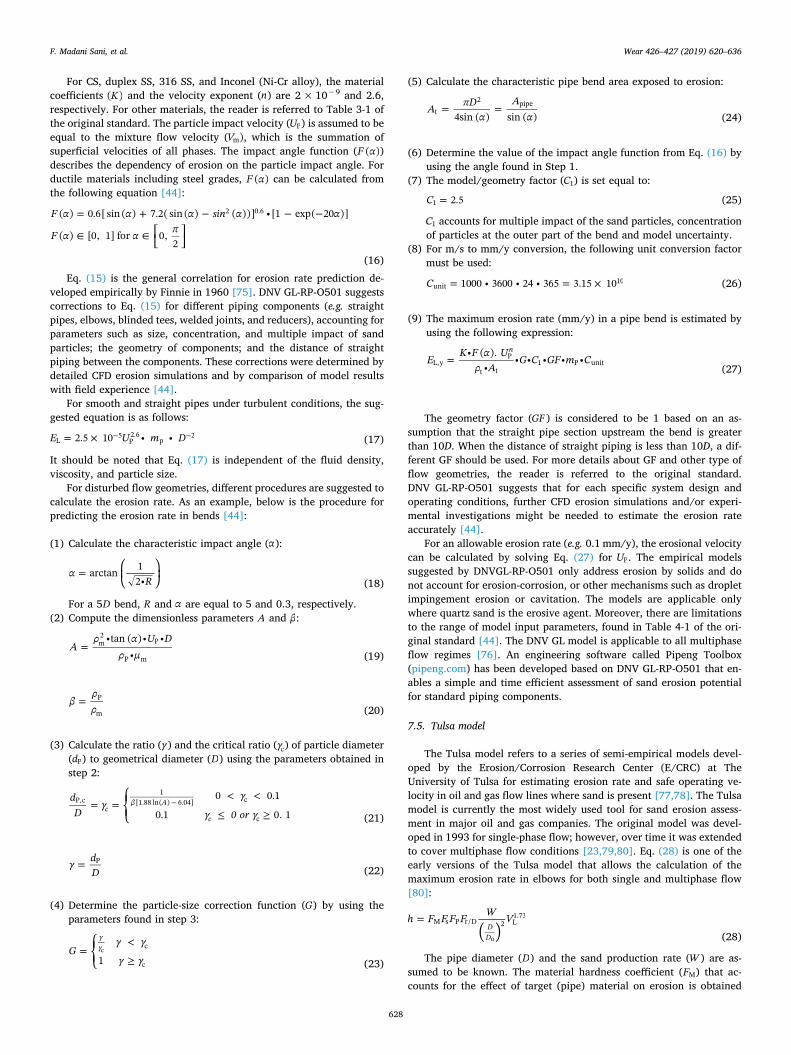
The characteristic particle impact velocity (VL) in Eq. (28) is theparticle velocity when the particle hits the pipe wall [82]. In order tocalculate VL in a complex pipe geometry such as a tee or an elbow, theerosion in that geometry was related to the erosion occurring in asimple 90° impingement situation [23,77,78]. Sand particles, beforeimpinging the pipe wall and causing erosion, enter a region near thewall in which their motion will be retarded by the fluid. This region iscalled the stagnation zone and its length is called the stagnation length[78,82]. Fig. 1 illustrates graphically the concepts of the stagnationzone and the stagnation length.

For a given pipe geometry, an equivalent stagnation length (L) wasdefined with reference to the stagnation length of a simple 90° im-pingement situation that will result in the same erosion rate as theaverage erosion rate in that geometry. L was determined by conductingerosion experiments for small pipe diameters followed by extrapolatingthe data to larger pipe diameters, using CFD simulations. For elbowsand tees, L can be calculated using the following semi-empiricalequations, respectively [79]:

= +

=

LL

tan D D

L in

1 1.27 (1.01 )

1.18o

1 1.89 0.129

o (31)

= +

=

LL

tan D D

L in

1.35 1.32 (1.63 )

1.06o

1 2.96 0.247

o (32)

Eqs. (31) and (32) are not applicable for diameters smaller than 1″ [80].A simplified particle tracking model was suggested to compute the

particle velocity profile along the stagnation zone (VP), assuming thatwhen a particle enters the stagnation zone it travels through a 1D-flowfield and only a drag force acts on the particle [23,77]:

= +dVd d

V V V VV

µ V VV dx

0.75 1 0.5( ) 24 ( )P

P

f

P

f P f p

P

f f P

P f P (33)

Vf in Eq. (33) is the fluid velocity along the stagnation zone, whichwas assumed to decrease linearly from the fluid bulk (average) velocity(Vo) at the beginning of the stagnation zone (x= 0) to zero at the targetwall (x= L) (See Fig. 1) [82]:

=V V xL

1f o (34)

Generally, Vp is not the same as Vf [82].VL is equal toVP at the pipe wall (x= L d

2P ) and can be determined

by solving Eq. (33) with a boundary condition of VP =Vo at =x 0. Fi-nally, the penetration rate (h) can be determined by substituting all theparameters explained above into Eq. (28).

In 2005, Oka et al. [83,84] proposed a new version of the Tulsamodel by assuming that erosion damage at an arbitrary impact angleE( ( )) is equal to the erosion damage at normal impact angle (E90)multiplied by a function (g ( )) that accounts for the effect of impactangle on the erosion damage. They expressed the erosion predictiveequation in terms of unit of material volume loss per mass of particles(mm3/kg) as follows:

=E g E( ) ( ) 90 (35)

=E K H VV

DD

( )kk k

90 VP P1

2 3

(36)

= +g H( ) (sin ) (1 (1 sin ))n n1V 2 (37)

= =n s H n s H( ) , ( )Vq

Vq

1 1 2 21 2 (38)

All parameters in the Oka et al. [83,84] model were obtained em-pirically. Table 6 shows the values of these parameters for a type ofsand (density= 2600 kg/m3) typically found in oil and gas fields.

Zhang et al. [85] in 2007 proposed a modified version of the Tulsamodel as presented below:

=ER CB F V F ( )s L0.59 2.41 (39)

The erosion ratio (ER) in Eq. (39) was defined as the ratio of targetmass loss to the total mass of particles impacting the target. The erosionratio can be converted to the penetration rate (h) by using the following

Table 3The values for B and C in Eq. (29) [59,79].

Material Brinell hardness (B) C

for VL in m/s for VL in ft/s

AISI 1018 210 1.95E-05 2.50E-06AISI 1020 150 1.94E-05 2.49E-0613Cr annealed 190 2.80E-05 3.59E-0613Cr heat treated 180 2.33E-05 2.98E-062205 duplex 217 1.88E-05 2.41E-06316 SS 183 1.98E-05 2.54E-06API Q125 290 1.95E-05 2.50E-06Incoloy 825 160 1.75E-05 2.24E-06

Table 4The particle shape coefficient (Fs) in Eq. (28) [23].

Particle shape Fs

Sharp corners (angular) 1.00Semi-rounded (rounded corners) 0.53Fully rounded 0.20

Table 5The penetration factor (FP) in Eq. (28) [59,81].

Geometry FP (for CS) FP (for SS316)

m/kg in/lb m/kg in/lb

90° elbow 0.206 3.68 0.631 11.26Tee 0.206 3.68 n/a n/aChoke 0.055 0.98 n/a n/aDirect impingement 0.224 4.00 n/a n/a

F. Madani Sani, et al. Wear 426–427 (2019) 620–636

629

equation:

=h ER F WD D( / )

P

o2 (40)

The material’s Brinell hardness in Eq. (39) was related to theVicker’s hardness by the equation below:

= +B H 0.10230.0108

V(41)

For the impact angle function (F ( )) in Eq. (39) a polynomialfunction was proposed by Zhang et al. [85] as follows:

==

F A( )i

i

0

5

i(42)

The values for empirical coefficients (Ai) and the corresponding Cconstant in Eq. (39) are given Table 7.

F(θ) depends on the target material, particle properties and flowconditions. F ( ) varies between zero and one. For ductile materialssuch as steels, different values have been reported for the impact angle( ) at which the maximum erosion occurs, ranging from 15° to 60°[24,69,75,76,85,87].

In 2009, Torabzadehkhorasani [88] and Okita [89] suggested a newversion of F ( ) based on the Oka et al. model (Eq. (37)):

= +Ff

sin H sin( ) 1 ( ) (1 (1 ))n n nV1 3 2

(43)

Table 8 summarizes f and ni in Eq. (43) and the corresponding Cconstant in Eq. (39) for different target materials and test conditions.The reader is encouraged to check the experimental details for each

case listed in Table 8 in order to establish a relevance for their case.There are other versions of the Tulsa model that came after Eq. (39),

such as Arabnejad et al. [69] and Shirazi et al. [95] versions. However,the most popular version of the Tulsa model at present is Eq. (39).

The early (Eq. (28)) and the new (Eq. (39)) versions of the Tulsamodel have the same form (see Eq. (40)) except for the impact anglefunction and the velocity exponent. The term Fr/D in the early versionseems to be substituted with F ( ) in the new version. Both terms ac-count for pipe geometry in erosion calculations. Moreover, it can beguessed that F ( ) in the early version of the Tulsa model was con-sidered to be 1, in order to give the maximum penetration rate.

When it comes to the velocity exponent in the Tulsa model, Zhang[96] observed that 1.73 over-predicted the erosion rate and suggestedto use 2.41 (along with a smaller C constant), instead. However, incertain cases acceptable results have been obtained by using 1.73 [81].The velocity exponent is an empirical value that varies with change inthe target material, particle properties and flow conditions. Vieira [81]reported velocity exponents of 2.71 and 2.77 for SS 316 in single-phaseair flow with 150 and 300 µm sand particles, respectively; or 2.93 forInconel 625 in the same flow with 300 µm sand particles. In anotherresearch, Vieira et al. [87] reported velocity exponents of 2.39 for300 µm and 2.49 for 150 µm sand particles in single-phase air flow.Mansouri [93] showed that in dry impact testing with single-phase airflow, 300 µm sand size and SS 316 target material, the velocity ex-ponent varied from 2.45 for 15° to 2.58 for 90° impact angle. However,2.41 was chosen as the velocity exponent for all pipe materials, sandparticles, and flow conditions in Eq. (39) and the C constant waschanged alternatively. The values for the C constant shown in Table 8are calculated by taking the average of the experimental results at aspecific test condition [93].

In the Tulsa model, it is suggested that for multiphase flow, the fluidmixture properties should be used wherever applicable. Mixture prop-erties such as mixture density and viscosity can be obtained from thefollowing equations:

=+

++

VV V

VV Vm

SL

SL SGL

SG

SL SGG (44)

=+

++

µ VV V

µ VV V

µLmSL

SL SG

SG

SL SGG (45)

The mixture velocity (Vm) in the API RP 14E equation and all thealternative models discussed in this article was assumed to be equal tothe average fluid velocity (Vo) and expressed as the summation of su-perficial liquid (VSL) and superficial gas (VSG) velocities [24,25,73,97]:

= = +V V V Vm o SG SL (46)

However, alternatively, a set of ad-hoc equations was also proposedfor the Tulsa model to calculate Vo in terms of VSL and VSG [97]:

= +V V V1n no L SL L SG (47)

Fig. 1. Graphical illustration of the stagnation zone and the stagnation length.Adopted from Ref. [80]. Vo is the fluid bulk (average) velocity; Vf is the fluidvelocity along the stagnation zone; L is the equivalent stagnation length or thelength of the stagnation zone in a direct 90° impingement geometry; and x is theparticle location along the stagnation zone.

Table 6Empirical constants and exponents in Eqs. (36)–(38) [83,84].

Particle K k1 k2 k3 s1 q1 s2 q2 V (m/s) D (μm)

SiO2-1 65 −0.12 2.3 H( )v 0.038 0.19 0.71 0.14 2.4 −0.94 104 326

Table 7Values of Ai in Eq. (42) and the corresponding C constant in Eq. (39).

Material C A0 A1 A2 A3 A4 A5 unit Ref.

Inconel 718 2.17E-07 0 5.4 −10.11 10.93 −6.33 1.42 Rad [85]SS 316 1.42E-07 −0.05065 0.04065 5.39E-04 −3.97E-05 5.14E-07 −2.07E-09 Degree [86]

F. Madani Sani, et al. Wear 426–427 (2019) 620–636

630

=+

VV VL

SL

SL SG

0.11

(48)

=n VV

1 exp 0.25 SG

SL (49)

In all the alternative models presented to this point, including theTulsa model, the quantification of erosion for multiphase flow is per-formed using the mixture fluid properties. These models do not considerthe multiphase-flow regimes in the erosion prediction calculations.Experiments showed that for an identical average fluid velocity inmultiphase flow, different flow regimes can lead to different erosionrates up to an order of magnitude. The main flow regimes in horizontalmultiphase lines are dispersed bubble, stratified, slug and annular-mistand in vertical multiphase lines are bubble, annular-mist, slug andchurn flow [82,98]. McLaury et al. [99] reported that the vertical or-ientation is 1.6–5 times more erosive than the horizontal orientation.Among the vertical flow regimes, the severity of erosion is highest inthe annular-mist flow [100]. Thus, the effect of flow regimes should beincorporated in modeling erosion for multiphase flow.

In multiphase flow, the interfacial forces between the phases, theproperties of the phases, the superficial velocities, flow orientation andpipe inclination angle are parameters that influence the flow regime.For various multiphase-flow regimes, the erosion models should differin the way they account for the characteristic particle impact velocity(VL). In erosion models that include the effect of flow regimes, thecharacteristic particle impact velocity is estimated based on the physicsinvolved in the given flow regime [82]. For example, in annular-mistflow the sand particles travelling in the gas core must pass through thethin liquid film at the pipe wall before impacting the wall and causingerosion. In slug flow, it is assumed that erosion is mainly caused by sandparticles uniformly distributed in the slug body [100]. For details onhow to calculate the characteristic particle impact velocity in differentmultiphase-flow regimes, the reader is referred to Refs. [101,102] forbubbly, Refs. [26,101–104] for annular, Refs. [26,101,105] for slug,and Refs. [100,101] for churn flow. For multiphase flow with ahomogeneous flow regime such as dispersed bubble, the mixture fluidproperties approach (Eqs. (44)–(46)) can be used for the erosion pre-diction calculations [106].

The Tulsa model can be used to estimate the erosional velocity if anallowable erosion rate (for example 5 or 10mpy) is specified. Theprocedure to determine the erosional velocity is outlined as follows:

(1) Establish an allowable erosion rate (e.g. 5 mpy).

(2) CalculateVL from Eq. (28) or Eq. (39) or any other erosion equationfrom the Tulsa model.

(3) Calculate L from Eq. (31) or Eq. (32).(4) Make an initial guess for Vo and plug it into Eq. (34) for Vf .(5) Plug Vf equation into Eq. (33) (or any other particle tracking

equation) and solve the final equation for VP with an initialboundary condition of VP=Vo at x= 0. If VP at the pipe wall( =x L d

2P ) equals toVL found in Step 2, then the initial guess ofVo is

considered as the erosional velocity. Otherwise, change the initialguess and repeat the procedure until the condition in step 5 is sa-tisfied.

The Tulsa model has advantages over other sand erosion modelsexplained in this paper when it comes to how it describes the erosionprocess. For example, it considers the reduction in the particle velocityas the particle moves through the fluid stagnation zone before im-pinging the pipe wall [59]; it accounts for many key factors in sanderosion including flow geometry type, size, and material; flow regimeand velocity; and sand shape, size and density [82].

However, the original Tulsa model has limitations as well. Thecalculation of the particle impact velocity is based on a 1D particletracking equation. In other words, only the particle velocity componentalong the stagnation length is considered for the calculations and theother two components that might be essential in erosion prediction arenot considered. In 2010, Zhang el at. [107] used a 2D particle trackingmethod for the Tulsa model. They reported that the 2D model agreedvery well with the experimental data from other researchers, while the1D model over predicted for most cases. In similar research, Zhang et al.[105] showed that in single-phase flow, the 1D model underpredictederosion caused by small particles (~20 µm), while predicted success-fully for relatively large particles (> 50 µm). In slug flow, they reportedthat the 1D model overpredicted erosion for the large particles; how-ever, it performed very well for the small particles. CFD simulations canbe used for a more accurate estimation of the particle impact velocityby including all three flow velocity components (3D particle trackingequation) [107].

The effect of turbulent dispersion of sand particles is not consideredin the original Tulsa model. This limits the model’s application to re-latively large sand particles (> 50–100 µm) and single-phase gas flowbecause large particles possess more momentum and are not affected bythe turbulence as much as small particles. Also, turbulent fluctuationsaffect particle motion less in gas flow comparing to liquid flow [107].Shirazi et al. [95] included the effect of turbulent flow in the Tulsa

Table 8Parameters used in Eqs. (39) and (43).

n1 n2 n3 Hv(GPa) f C(metric units) Target material conditions Ref. (year)

1.40 1.64 2.60 1.50 1.72 1.42E-07 SS 316 Air/sand (150 µm) [89] (2010)0.59 3.60 2.50 1.20 5.27 1.50E-07 Al 6061 Air/sand (150 µm)0.50 2.50 0.50 1.20 2.19 3.28E-07 Al 6061 Air/sand (300 µm)1.90 0.96 35 1.10 3.25 2.55E-07 Al 6061 Air/glass beads (50 µm) [90] (2011)0.85 0.60 44 1.09 3.67 4.65E-07 Al 6061 Air/glass beads (150 µm)1.38 0.68 44 1.09 3.64 2.80E-07 Al 6061 Air/glass beads (350 µm)0.40 0.80 3.00 1.52 1.71 2.20E-07 SS 316 Air/sand (300 µm) [81] (2014)0.60 0.50 2.80 2.27 1.64 3.41E-07 Inconel 625 Air/sand (300 µm)0.65 1.40 1.50 2.74 3.46 (2.72 ± 0.44)E-07 22Cr Air/sand (300 µm)0.50 1.40 1.20 1.92 2.05 (1.88 ± 0.79)E-07 13Cr Duplex Air/sand (300 µm)0.98 1.70 2.91 1.72 4.13 (2.36 ± 0.44)E-07 1018 CS Air/sand (300 µm)0.40 1.50 2.50 1.44 2.81 (2.25 ± 0.14)E-07 4130 CS Air/sand (300 µm)0.60 2.20 13 1.09 5.94 (1.36 ± 1.44)E-07 Al 6061 Air/sand (300 µm)0.40 0.80 3.00 1.52 1.71 (3.08 ± 0.39)E-07 SS 316 Air/sand (300 µm) [91] (2014)0.20 0.85 0.65 1.83 1.71 4.49E-07 SS 316 Water/sand (300 µm) [92] (2015)0.20 0.85 0.65 1.83 1.43 4.92E-07 SS 316 Air/sand (300 µm) [93] (2016)1.52 8.90 0.01 1.83 18.74 2.04E-07 SS 316 Water/sand (300 µm)0.15 0.85 0.65 1.83 1.54 4.62E-07 SS 316 Air/sand (300 µm) [87] (2016)0.40 0.80 2.08 1.83 1.72 1.14E-08 SS 316 Air/sand (150 and 300 µm) [94] (2016)

F. Madani Sani, et al. Wear 426–427 (2019) 620–636

631

model (Eq. (28)) by introducing another velocity component thatcharacterizes motion of eddies in the flow stream or in the turbulentboundary layer close to the wall. They claimed that this new modelshowed a relatively good agreement between the experimental andcalculated results for single and multiphase flow, except for few cases inannular flow, which was probably because the effect of liquid film wasnot considered in the model [95].

The Tulsa model relies on empirical equations to account for theparticle size and shape, and material target in erosion prediction cal-culations. However, these equations are not always accurate [69]. Asshown in Table 8, for similar erodent particle and target material dif-ferent C constants have been incorporated into the final erosion equa-tion (Eq. (39)). Even with the same parameters for the impact anglefunction, different C constants have been considered for Eq. (39)(compare rows 7 and 14 of Table 8).

Finally, the original Tulsa model is mainly limited to simple geo-metries such as elbows and tees and single-phase carrier fluid such asgas or liquid [95]. For complex geometries and multiphase flow, CFDcodes have been employed in the Tulsa model, primarily for calculatingthe particle impact velocity (VL). The CFD-based models — CFD codeslinked with empirical erosion equations — can be used for developingsimplified models for erosion prediction in complex geometries andmultiphase flow. Zhang et al. [107] in 2010 claimed that while CFD-based models are powerful tools, they require too much computationaleffort, and therefore, are not practical for engineering applications.However, with the constant advancement of CFD software packagesand faster computers, CFD techniques are rapidly becoming a main-stream tool fully available to practicing engineers. Therefore, this ar-gument may not carry as much weight today as it did 10 years ago.

7.6. Shell model

The Shell model also called the Reduced Order model was devel-oped around 1997 based on the Tulsa model for estimating the erosionrate and the erosional velocity in multiphase flow. In the Shell model,Eq. (28) was used for the sand erosion rate calculations with two main

simplifications. First, instead of Eq. (33) for calculating the impactparticle velocity which requires significant numerical computation tosolve, a simpler particle tracking equation was offered [59]:

= ++Re Re

VV

1 10.147 23.62 11

P

f

2

6 (50)

The two dimensionless numbers: (mass ratio) and Re (particleReynolds number) in Eq. (50) are as below [59]:

=ReV dµ

f Pf

f (51)

=L

df

P P (52)

The second simplification was setting the total erosion rate equal tothe summation of the erosion rate caused by each phase. An effectivepipe diameter (Deff ) was defined for each phase in order to calculate theerosion rate for that phase. The following equation is the effective pipediameter for the liquid phase:

=+

D ID QQ Qeff,L

L

L G

12

(53)

A similar equation can be used for the gas phase [59].The phase separation assumption was not entirely correct because

for low liquid flow rates (small QL) like annular-mist flow, Deff,L will besmall, which literally means there is no stagnation zone (it is a functionof the diameter), while for high liquid flow rates the effect of stagnationzone will be considerable [59].

8. Comparison of erosion models

Fig. 2 uses the box-and-whisker plot format to present the ratio ofcalculated to experimentally measured erosion in the presence of solids.A value of 1 for the ratio (indicated on the y-axis) represents perfectagreement. Above 1 indicates that the erosion model overpredicts the

Fig. 2. The ratio of calculated to measured erosion in the presence of solids shown by box-and-whisker plots (min, quartile 1, median, quartile 3 and max). Each boxrepresents a separate set of experimental data compared with an erosion model. 1D and 2D indicate one and two-dimensional equations of motion used in the Tulsamodel, respectively. The description of each model and the Refs. data taken from: Salama: Eq. (14) [76,95,97]; DNV GL: Eqs. (18)–(27) [44,76,87,97]; Old Eq. 1D:Eq. (28), flow-regime independent [76,97]; Old + Ad-hoc Eqs.: Eq. (28) and Eqs. (47)–(49) [97]; Oka et al.: Eqs. (35)–(38) [87,97]; New Eq. 2D: Eq. (39), based onZhang et al. [107] [76,87,97]; CFD + New Eq.: CFD codes + Eq. (39), based on Zhang et al. [85] [3,86,87,89,92,94,97]; Annular + Old Eq.: Eq. (28), based onMazumder et al. [100,101] [26,97,103,108]; Annular + New Eq.: Eq. (39), based on Zahedi et al. [103]; Slug 1D: Eq. (28), based on Mazumder et al. [100,101][26,105]; Slug 2D: Eq. (39), based on Zhang et al. [105]; Arabnejad et al.: based on Arabnejad et al. [69] [3,97]; Shirazi et al.: turbulent model, based on Shirazi et al.[95].

F. Madani Sani, et al. Wear 426–427 (2019) 620–636

632

corresponding experimental data and vice versa. Overprediction oferosion corresponds to a lower erosional velocity limit, implying thatthe model is conservative. Conversely, underprediction of erosiontranslates to a higher erosional velocity limit, which may lead to riskydecisions. The experimental values presented in Fig. 2 are generated bya statistical analysis of data gathered from various publications in theopen literature. Each box corresponds to a separate set of erosion ex-perimental data that is compared with the corresponding erosion valuescalculated by a given model.

Three groups of erosion calculations are shown in Fig. 2: the Salamamodel, the DNV GL model, and different versions of the Tulsa model.The Salama model overpredicted the experimental data in almost allcases (often by one order of magnitude or more), and hence can beconsidered quite conservative. The DNV GL model showed similar ac-curacy (within an order of magnitude); however, the underpredictionwas frequent and presents a potential risk as it can lead to an over-estimation of the erosional velocity.

When it comes to different versions of the Tulsa model, Fig. 2 showsthat both “Old Eq. 1D” and “New Eq. 2D” models tended to overpredicterosion, performing in general similarly to Salama model. However, thedispersion of the “Old Eq. 1D” predictions was less than that for the“New Eq. 2D” model, suggesting that it is somewhat more accurate.This conclusion is at odds with Zhang et al. [107]’s claim that the “NewEq. 2D” model predicts erosion behavior much better than the “Old Eq.1D” model. Recall that the “Old + Ad-hoc Eqs.” model is the same asthe “Old Eq. 1D” model except that Eqs. (47)–(49) are used instead ofEq. (46) for calculating the fluid bulk velocity. The single data set usedfor the evaluation of the “Old + Ad-hoc Eqs.” model shows that itunderpredicted the experimental results. However, more data are re-quired to make a more accurate conclusion about the accuracy of thismodel. Even though the Oka et al. model appears to be relatively ac-curate, it underpredicted most of the erosion data, which makes themodel less safe for practical purposes.

The “CFD + New Eq.” model refers to the Tulsa model in whichCFD codes were used for flow modeling and particle tracking, and Eq.(39) was used for erosion prediction. As mentioned above, this type ofmodel is the most commonly used version of the Tulsa model as is in-dicated in the open literature. The Zhang et al. [85] model is the basisof the “CFD +new Eq.” model. The exact CFD packages used in the“CFD + New Eq.” models are not explicitly referenced in the originalpublications. It is possible that the boxes in Fig. 2 for the “CFD + NewEq.” models are based on different CFD packages, such as FLUENT, CFXor STAR-CCM+, which may be the source of difference in the results.Fig. 2 shows that the “CFD + New Eq.” models underpredicted theexperimental data for the majority of cases (considering the median)and in some cases the spread was unacceptably large. Several re-searchers reported that the CFD-based Tulsa models underpredicted theexperimental erosion data [85,86,89,92], e.g. Zhang et al. [85] andOkita [89] mentioned that the CFD-based Tulsa model underpredictedthe experimental data as the viscosity of the carrier fluid increases.

When it comes to different multiphase flow regimes, both Annularmodels predicted the experimental data relatively well with an order ofmagnitude accuracy. For both Slug models, the ratio of calculated tomeasured erosion scattered significantly, with the Slug 2D model beingmore accurate than the Slug 1D model.

In summary, among all the models presented in Fig. 2, it appearsthat the Arabnejad et al. [69] and Shirazi et al. [95] models were themost accurate and suitable models for estimating the erosional velocity,which is not a surprise as they are the most recent models presented bythis group.

Some of the erosion models discussed above were used for a hy-pothetical case (with conditions listed in Table 9) to compare the ero-sional velocity calculated by them with that estimated by the API RP14E equation.

Fig. 3 shows the results of such a comparison for a given allowableerosion rate of 5mpy. Above and to the right of each curve indicates

velocities resulting in the erosion rate being greater than 5mpy, andvice versa. Where the complete descriptions of the erosion models weregiven in the open literature, i.e. for the API RP 14E, Salama, and DNVGL models, the models were recreated and used for the erosional ve-locity calculations. For the Tulsa model, the SPPS 1D software version5.3. was used. For the Shirazi et al. (turbulent) model, because of theincomplete information available in the public domain, data were takendirectly from the source publication [95]. The comparison for theShirazi et al. model might not be completely correct because not all theinput conditions listed in Table 9 were mentioned in the source pub-lication.

The comparison shows that the API RP 14E equation is the mostconservative model for high liquid superficial velocities (flow lines witha considerable amount of liquid). At these conditions, the API RP 14Eerosional velocity amounting to a total velocity of approximately10–20 ft/s corresponds roughly to the transition from slug to dispersedbubble flow, as shown in the flow regime map in Fig. 4 (and as graydotted lines in Fig. 3), generated for the same conditions. While thismight be a coincidence, it makes little sense to limit the velocity so thatthe flow regime does not transit from slug (which is generally con-sidered to be the most violent) to dispersed bubble (which is thought asone of the most benign). At high liquid superficial velocities, the Salamamodel allows the highest operating velocities, yet at unrealistic levels,where other operational restrictions must apply. The DNV GL, Tulsaand Shirazi et al. models predict the erosional velocity somewhere inbetween the API RP 14E equation and the Salama model.

Conversely, at high superficial gas velocities and low superficialliquid velocities (flow lines with a considerable amount of gas and asmall amounts of liquid), the API RP 14E equation allows the highestvelocity and is actually the least conservative model, while the Salamaand Shirazi et al. models are the most conservative models, with theothers being in between. This is probably the reason for recommending50% of the API RP 14E erosional velocity as the safe operating velocityfor gas pipelines [109]. From comparisons with the flow regime map(Fig. 4) it appears that most of the models restrict the transition to theannular-mist flow regime, which is logical as the high gas velocitiesmay lead to significant levels of droplet and sand impingement. How-ever, this could be just a coincidence, as most of the models do notexplicitly account for the effect of various two-phase flow regimes.

Table 9Parameters for calculation of the erosional velocity.

Parameter Value Unit Description

Operating pressure 514.7 psia –Operating temperature 100 °F –Carrier fluids – – Water and methaneWater cut 1 – Ratio of water to total liquidGas specific gravity 0.55 – SgGas density 1.445 lb/ft3 –Gas viscosity 0.033 cp –Liquid specific gravity 1 – SlLiquid density 62.01 lb/ft3 –Liquid viscosity 0.682 cp –Gas compressibility 0.998 –Gas-liquid surface tension 7.21 dyne/cm –Pipe geometry – – Seamless long radius elbowMaterial – – Carbon steelMaterial density 486.94 lb/ft3 –Pipe diameter 4 in –Radius of curvature 5 – –Material hardness 140 B BrinellPipe roughness 20 µm –Sand feed rate 10 lb/day –Sand size 150 μm –Sand shape – – Semi-roundedSand density 162.31 lb/ft3 –

F. Madani Sani, et al. Wear 426–427 (2019) 620–636

633

9. Current oilfield approaches

Current oilfield practices generally combine several of the ap-proaches discussed previously:

• For non-corrosive fluids without solids, any restrictions due topossible erosion are not a limiting factor, i.e. the API RP 14Eequation that is actually defined for this type of service, is not used.• The effect of flow for the case of transportation of corrosive fluidswithout solids (FIC/FAC scenario) are covered by existing corrosionmodels (such as MULTICORP™, OLI Systems, ECE®, Thermo-Calc,etc.).• For non-corrosive fluids with solids (erosion scenario), instead ofusing the API RP 14E equation with a reduced c-factor, the alter-natives, such as the DNV GL or the Tulsa erosion models aresometimes used. In special cases with more complicated geometries,more advanced CFD models are used.• For corrosive fluids with solids (case of erosion-corrosion), specificstudies are often performed or field experience may be applied whenavailable. Although researchers have been trying to model thecombined process of erosion and corrosion [11,67,110–115], sincethe mechanism for erosion-corrosion is still not fully understood this

area needs further improvement. Rules of thumb and simple em-pirical guidelines are used in most applications. These often amountto specifying the erosional velocity directly or using simple criteriain the forms of decision tables or flowcharts on how to determinethe limiting velocity. The rules and guidelines differ from companyto company. They are based on operational conditions such asconcentration of solids, type of service, corrosiveness of the fluid,and presence of corrosion inhibitors.

10. Conclusions

• The widespread use of the API RP 14E erosional velocity equation isa result of its simplicity and requiring little in the way of inputs.However, the API RP 14E equation does not account for most of thefactors important in erosion, FIC/FAC and erosion-corrosion.• The origin of the API RP 14E erosional velocity equation remainsunclear. The theoretical explanations (e.g. energy balance, Bernoulliequation, liquid droplet impingement, and corrosion inhibitor/pro-duct removal) that supposedly underpin the derivation of the API RP14E equation do not seem to properly justify its form. The alter-native explanations involving anecdotal evidence on empiricalorigin of the API RP 14E equation are even less convincing.• There is a problematic assumption (often implicit) that the API RP14E equation can be used as a means of generalizing observed em-pirical erosion, FIC/FAC or erosion-corrosion data to derive safeoperational velocities for a broad variety of conditions, usuallyoutside operational or experimental ranges. This assumption ignoresthe fact that the mechanism and the rate of degradation can be verydifferent (by orders of magnitude) depending on type of service oreven within the same type of service.• The API RP 14E equation cannot be simply applied to all kinds ofconditions by just modifying the c-factor, assuming that it is uni-versally valid and it will give reasonable values.• Despite its widespread use, the API RP 14E equation has manylimitations. Probably the most significant is that it does not provideany quantitative guidelines for limiting the velocity in the two mostcritical scenarios: when solid particles are present in the productionfluids (erosion) and when erosion and corrosion are both an issue(erosion-corrosion). A reduction in the c-factor is recommended byAPI RP 14E, although it is unclear how to obtain the exact value.• Some of the alternative approaches overlap with and in some as-pects go beyond the narrow application range of the API RP 14Eerosional velocity equation. Examples are the NORSOK P-002standard [68] and to some extent the recommendations of Sve-deman and Arnold [63]. In other cases, the alternatives focus onhow to derive velocity limits in the presence of solid particles, be-yond just arbitrarily using the API RP 14E erosional velocity equa-tion with a smaller c-factor. The best-known examples are theSalama model, the DNV GL model, and various versions of the Tulsamodel.• When it comes to the complicating effect of combined erosion-cor-rosion attack, researchers have been pursuing the so called erosion-corrosion mapping approach [66,110,112]. However, in the appli-cations, rules-of-thumb and simple empirical guidelines are used inmost cases.

Acknowledgments

The authors would like to gratefully acknowledge the constructivehelp of Dr. Michel Bonis (TOTAL); Dr. Bruce Brown, Dr. David Young,and Dr. Luciano Paolinelli (Institute for Corrosion and MultiphaseTechnology); Mr. Kamal Pakdaman (BACO for Oil IndustryConstruction, Basra), and Mr. Hossein Jafari (Iranian OffshoreEngineering and Construction Company) during the writing of this re-view paper.

Fig. 3. Comparison of erosional velocity curves calculated by the API RP 14equation and other models based on conditions listed in Table 9. Data for theShirazi et al. model are taken from Ref. [95]. The gray dotted lines present theflow regime map shown in Fig. 4. For the API RP 14E equation, the ideal gaslaw was used to convert the gas velocity at operating conditions to that atstandard conditions and the gas/liquid ratio at standard conditions (R) wasassumed to be equal to V5.61( /Vsg sl) (see the Supplementary Materials for detailson calculations).

Fig. 4. The flow regime map for a 4-in vertical pipe operating at conditionslisted in Table 9. Calculated with MULTICORP™ 5.5.0.

F. Madani Sani, et al. Wear 426–427 (2019) 620–636

634

Appendix A. Supporting information

Supplementary data associated with this article can be found in theonline version at https://doi.org/10.1016/j.wear.2019.01.119.

References

[1] B.S. McLaury, J. Wang, S.A. Shirazi, J.R. Shadley, E.F. Rybicki, Solid particleerosion in long radius elbows and straight pipes, in: Soc. Pet. Eng., 1997. https://doi.org/10.2118/38842-MS.

[2] M.M., Salama, E.S., Venkatesh, Evaluation of API RP 14E erosional velocity lim-itations for offshore gas wells, in: Proceedings of the Offshore TechnologyConference, Houston, TX, 1983: Paper No. OTC-4485-MS. ⟨https://doi.org/10.4043/4485-MS⟩.

[3] H. Arabnejad, A. Mansouri, S.A. Shirazi, B.S. McLaury, Abrasion erosion modelingin particulate flow, Wear 376–377 (Part B) (2017) 1194–1199, https://doi.org/10.1016/j.wear.2017.01.042.

[4] D. Lusk, M. Gupta, K. Boinapally, Armoured against corrosion, Hydrocarb. Eng.(2008).

[5] A. Thiruvengadam, Erosion, Wear, and Interfaces with Corrosion, ASTMInternational, Philadelphia, PA, 1982.

[6] F.J. Heymann, Liquid impingement erosion, in: Frict. Lubr. Wear Technol.American Society for Metals International, 1992, pp. 221–232.

[7] R.J.K. Wood, Erosion–corrosion interactions and their effect on marine and off-shore materials, Wear 261 (2006) 1012–1023, https://doi.org/10.1016/j.wear.2006.03.033.

[8] D.C. Silverman, Rotating cylinder electrode — geometry relationships for pre-diction of velocity-sensitive corrosion, Corrosion 44 (1988) 42–49, https://doi.org/10.5006/1.3582024.

[9] E. Heitz, Chemo-mechanical effects of flow on corrosion, Corrosion 47 (1991)135–145, https://doi.org/10.5006/1.3585229.

[10] K.J. Kennelley, R.H. Hausler, D.C. Silverman, Flow-Induced Corrosion:Fundamental Studies and Industry Experience, NACE, Houston, TX, 1992.

[11] J.R. Shadley, S.A. Shirazi, E. Dayalan, E.F. Rybicki, Prediction of erosion-corrosionpenetration rate in a carbon dioxide environment with sand, Corrosion 54 (1998)972–978, https://doi.org/10.5006/1.3284819.

[12] R. Barker, X. Hu, A. Neville, S. Cushnaghan, Flow-induced corrosion and erosion-corrosion assessment of carbon steel pipework in oil and gas production, in:Corrosion, NACE International, Houston, TX, 2011, p. 11245.

[13] M.M. Stack, B.D. Jana, S.M. Abdelrahman, 6- Models and mechanisms of ero-sion–corrosion in metals, in: Proceedings of the Tribocorrosion Passive Met. Coat.,1st ed., Woodhead Publishing, 2011, pp. 153–187. ⟨https://doi.org/10.1533/9780857093738.1.153⟩.

[14] R.J.K. Wood, S.P. Hutton, The synergistic effect of erosion and corrosion: trends inpublished results, Wear 140 (1990) 387–394, https://doi.org/10.1016/0043-1648(90)90098-U.

[15] R. Malka, S. Nesic, D.A. Gulino, Erosion–corrosion and synergistic effects in dis-turbed liquid-particle flow, Wear 262 (2007) 791–799, https://doi.org/10.1016/j.wear.2006.08.029.

[16] M.M. Stack, S. Zhou, R.C. Newman, Identification of transitions in erosion-cor-rosion regimes in aqueous environments, Wear 186–187 (1995) 523–532, https://doi.org/10.1016/0043-1648(95)07175-X.

[17] S. Hassani, K.P. Roberts, S.A. Shirazi, J.R. Shadley, E.F. Rybicki, C. Joia, Flow loopstudy of NaCl concentration effect on erosion, corrosion, and erosion-corrosion ofcarbon steel in CO2-saturated systems (026001.1-026001.9), Corrosion 68 (2012),https://doi.org/10.5006/1.3683229.

[18] Y. Zheng, Z. Yao, X. Wei, W. Ke, The synergistic effect between erosion and cor-rosion in acidic slurry medium, Wear 186–187 (1995) 555–561, https://doi.org/10.1016/0043-1648(95)07132-6.

[19] S. Hassani, K.P. Roberts, S.A. Shirazi, J.R. Shadley, E.F. Rybicki, C. Joia, A newapproach for predicting inhibited erosion-corrosion in CO2-saturated oil/brineflow condition, SPE Prod. Oper. 28 (2013) 135–144, https://doi.org/10.2118/155136-PA.

[20] S. Hassani, K.P. Roberts, S.A. Shirazi, J.R. Shadley, E.F. Rybicki, C. Joia,Characterization and prediction of chemical inhibition performance for erosion-corrosion conditions in sweet oil and gas production, Corrosion 68 (2012)885–896, https://doi.org/10.5006/0546.

[21] H. Arabnejad, S.A. Shirazi, B.S. McLaury, J.R. Shadley, Calculation of ErosionalVelocity Due to Liquid Droplets with Application to Oil and Gas IndustryProduction, in: Society of Petroleum Engineers, New Orleans, LA, 2013, , https://doi.org/10.2118/166423-MS.

[22] J.R. Shadley, E.F. Rybicki, S.A. Shirazi, E. Dayalan, Velocity guidelines foravoiding erosion-corrosion damage in sweet production with sand, J. EnergyResour. Technol. 120 (1998) 78–83, https://doi.org/10.1115/1.2795014.

[23] S.A. Shirazi, B.S. McLaury, J.R. Shadley, E.F. Rybicki, Generalization of the API RP14E guideline for erosive services, J. Pet. Technol. 47 (1995) 693–698, https://doi.org/10.2118/28518-PA.

[24] M.M. Salama, An alternative to API 14E erosional velocity limits for sand ladenfluids, J. Energy Resour. Technol. 122 (2000) 71–77, https://doi.org/10.4043/8898-MS.

[25] API RP 14E, recommended practice for design and installation of offshore pro-duction platform piping systems, American Petroleum Institute, 5th ed., 1991.

[26] B.S. McLaury, S.A. Shirazi, E.F. Rybicki, Sand erosion in multiphase flow for slugand annular flow regimes, in: Corrosion, NACE International, San Antonio, TX,

2010, p. 10377.[27] H. Mansoori, F. Esmaeilzadeh, D. Mowla, A.H. Mohammadi, Case study: produc-

tion benefits from increasing C-values, Oil Gas J. (2013).[28] S.R. Mofrad, Erosional velocity limit, 2014.[29] R. Russell, S. Shirazi, J. Macrae, A New Computational Fluid Dynamics Model to

Predict Flow Profiles and Erosion Rates in Downhole Completion Equipment, in:Society of Petroleum Engineers, Houston, TX, 2004, , https://doi.org/10.2118/90734-MS.

[30] H. Arabnejad, S.A. Shirazi, B.S. McLaury, J.R. Shadley, A Guideline to CalculateErosional Velocity Due to Liquid Droplets for Oil and Gas Industry, in: Society ofPetroleum Engineers, Amsterdam, Netherlands, 2014.

[31] M.M. Salama, Erosion velocity limits for water injection systems, Mater. Perform.32 (1993) 44–49.

[32] J.M. Coulson, J.F. Richardson, Chemical Engineering, Vol. 1: SI Units, 3rd ed.,Pergamon Press, 1977.

[33] U. Lotz, Velocity effects in flow induced corrosion, in: Corrosion, NACEInternational, Las Vegas, NV, 1990, p. 27.

[34] C.E. Brennen, Chapter 5- Cavitation parameters and inception, in: Hydrodynamicsof Pumps, Cambridge University Press, 2011, pp. 55–77, , https://doi.org/10.1017/CBO9780511976728.007.

[35] M. Dular, B. Stoffel, B. Sirok, Development of a cavitation erosion model, Wear261 (2006) 642–655, https://doi.org/10.1016/j.wear.2006.01.020.

[36] W. Li, B.F.M. Pots, X. Zhong, S. Nesic, Inhibition of CO2 corrosion of mild steel –Study of mechanical effects of highly turbulent disturbed flow, Corros. Sci. 126(2017) 208–226, https://doi.org/10.1016/j.corsci.2017.07.003.

[37] S. Hattori, M. Takinami, Comparison of cavitation erosion rate with liquid im-pingement erosion rate, Wear 269 (2010) 310–316, https://doi.org/10.1016/j.wear.2010.04.020.

[38] F. Cheng, W. Ji, C. Qian, J. Xu, Cavitation bubbles dynamics and cavitation erosionin water jet, Results Phys. 9 (2018) 1585–1593, https://doi.org/10.1016/j.rinp.2018.05.002.

[39] T. Shakouchi, K. Kinoshita, K. Tsujimoto, T. Ando, Flow-accelerated corrosion inpipe wall downstream of orifice for water and air-water bubble flows, J. Flow.Control Meas. Vis. 04 (2016) 93, https://doi.org/10.4236/jfcmv.2016.43009.

[40] B. Craig, Critical velocity examined for effects of erosion-corrosion, Oil Gas J. 83(1985) 99–100.

[41] J.S. Smart, The meaning of the API RP 14E formula for erosion corrosion in oil andgas production, in: Corrosion, NACE International, Cincinnati, OH, 1991, p. 468.

[42] H. Arabnejad, A. Mansouri, S.A. Shirazi, B.S. McLaury, J.R. Shadley, Erosion-corrosion study of oil-field materials due to liquid impact, in: Corrosion, NACEInternational, Dallas, TX, 2015, p. 6136.

[43] D.M. Deffenbaugh, J.C. Buckingham, A Study of the Erosional Corrosional VelocityCriterion for Sizing Multi-phase Flow Lines, Phase I, Southwest Research Institute,Reston, VA, 1989.

[44] DNVGL-RP-O501, recommended practice: managing sand production and erosion,Det Norske Veritas, 2015.

[45] M.H. Chaudhry, Applied Hydraulic Transients, 3rd ed., Springer Science &Business Media, 2013.

[46] R.H. Hausler, C. Consulta, G. Schmitt, Hydrodynamic and flow effects on corrosioninhibition, in: Corrosion, NACE International, New Orleans, LA, 2004, p. 04402.

[47] Y. Xiong, B. Brown, B. Kinsella, S. Nesic, A. Pailleret, Atomic force microscopystudy of the adsorption of surfactant corrosion inhibitor films, Corrosion 70 (2013)247–260, https://doi.org/10.5006/0915.

[48] W. Li, B.F.M. Pots, B. Brown, K.E. Kee, S. Nesic, A direct measurement of wallshear stress in multiphase flow—Is it an important parameter in CO2 corrosion ofcarbon steel pipelines? Corros. Sci. 110 (2016) 35–45, https://doi.org/10.1016/j.corsci.2016.04.008.

[49] S. Nesic, Effects of multiphase flow on internal CO2 corrosion of mild steel pipe-lines, Energy Fuels 26 (2012) 4098–4111, https://doi.org/10.1021/ef3002795.

[50] J.S. Smart, A review of erosion corrosion in oil and gas production, in: Corrosion,NACE International, Las Vegas, NV, 1990, p. 10.

[51] J.A. Keeth, Some corrosion problems encountered in steam plant operations,Corrosion 11 (1946) 101–124.

[52] P. Andrews, T.F. Illson, S.J. Matthews, Erosion–corrosion studies on 13 Cr steel ingas well environments by liquid jet impingement, Wear 233–235 (1999) 568–574,https://doi.org/10.1016/S0043-1648(99)00228-8.

[53] M.J. Castle, D.T. Teng, Extending gas well velocity limits: problems and solutions,in: Proceedings of the Soc. Pet. Eng. SPE, Perth, Western Australia: 1991, pp.135–144.

[54] R. Heidersbach, Velocity Limits for Erosion-Corrosion, in: Dallas, TX, 1985.[55] C.C. Patton, Are we out of the iron age yet? in: Corrosion, NACE International,

Houston, TX, 1993, p. 93056.[56] D. Panic, J. House, Challenging conventional erosional velocity limitations for

high rate gas wells, in: 2009, p. 6.[57] M.A. Ariana, F. Esmaeilzadeh, D. Mowla, Beyond the limitations of API RP-14E

erosional velocity - a field study for gas condensate wells, Phys. Chem. Res. 6(2018) 193–207, https://doi.org/10.22036/pcr.2017.93963.1403.

[58] Annual report to Alaska department of environmental conservation: commitmentto corrosion monitoring, Corrosion, Inspection and Chemicals (CIC) Group, BPExploration (Alaska) Inc., 2002.

[59] K. Jordan, Erosion in multiphase production of oil & gas, in: Corrosion, NACEInternational, San Diego, California, 1998, p. 5834.

[60] M. Bonis, Private technical communication, TOTAL, 2018.[61] J.H. Gerretsen, A. Visser, Inhibitor performance under liquid droplet impingement

conditions in CO2-containing environment, Corros. Sci. 34 (1993) 1299–1310,https://doi.org/10.1016/0010-938X(93)90089-Y.

F. Madani Sani, et al. Wear 426–427 (2019) 620–636

635

[62] API Specification 5CT, Specification for Casing and Tubing, 10th ed., AmericanPetroleum Institute, 2018.

[63] S.J. Svedeman, K.E. Arnold, Criteria for sizing multiphase flowlines for erosive/corrosive service, SPE Prod. Facil 9 (1994) 74–80, https://doi.org/10.2118/26569-PA.

[64] U.R. Richard, Sand and Fines in Multiphase Oil and Gas Production (Master’sthesis), Norwegian University of Science and Technology, Trondheim, Norway,2013.

[65] A.T. Salazar, Erosional velocity limitations for oil and gas wells - extracted fromNeotec Wellflow Manual, 2012.

[66] C.B. Burson-Thomas, R.J.K. Wood, Developments in erosion–corrosion over thepast 10 Years, J. Bio- Tribo Corros. 3 (2017) 14, https://doi.org/10.1007/s40735-017-0073-4.

[67] M.M. Stack, B.D. Jana, Modelling particulate erosion–corrosion in aqueous slur-ries: some views on the construction of erosion–corrosion maps for a range of puremetals, Wear 256 (2004) 986–1004, https://doi.org/10.1016/j.wear.2003.09.004.

[68] NORSOK P-002, Process system design (Revision 1), Standards Norway (SN),2014.

[69] H. Arabnejad, A. Mansouri, S.A. Shirazi, B.S. McLaury, Development of mechan-istic erosion equation for solid particles, Wear 332–333 (2015) 1044–1050,https://doi.org/10.1016/j.wear.2015.01.031.

[70] International Standard, ISO 13703: petroleum and natural gas industries—designand installation of piping systems on offshore production platforms, 2000.

[71] Specifications for salt water piping systems in ships (BS MA18: 1973), BritishStandards Institution.1976.

[72] A.T.J. Bourgoyne, Experimental study of erosion in diverter systems due to sandproduction, in: Soc. Pet. Eng., 1989, pp. 807–816. https://doi.org/10.2118/18716-MS.

[73] S.J. Svedeman, A Study of the Erosional/Corrosional Velocity Criterion for SizingMultiphase Flow Lines, Phase II, Southwest Research Institute, Reston, VA, 1990.

[74] A. Huser, O. Kvernvold, Prediction of sand erosion in process and pipe compo-nents, in: Proceedings of the 1st North Am. Conference Multiph. Technol., Banff,Canada: 1998: pp. 217–227.

[75] I. Finnie, Erosion of surfaces by solid particles, Wear 3 (1960) 87–103, https://doi.org/10.1016/0043-1648(60)90055-7.

[76] H. Arabnejad, A. Mansouri, S.A. Shirazi, B.S. McLaury, Evaluation of solid particleerosion equations and models for oil and gas industry applications, in: Proceedingsof the Soc. Pet. Eng., Society of Petroleum Engineers, Houston, TX: 2015, PaperNo. SPE-174987-MS. ⟨https://doi.org/10.2118/174987-MS⟩.

[77] B.S. McLaury, S.A. Shirazi, J.R. Shadley, E.F. Rybicki, A particle tracking methodto predict sand erosion threshold velocities in elbows and tees, in: Proceedings ofthe ASME Fluids Eng. Div., Lake Tahoe, Nevada, 1:994, pp. 145–154.

[78] S.A. Shirazi, J.R. Shadley, B.S. McLaury, E.F. Rybicki, A procedure to predict solidparticle erosion in elbows and tees, J. Press. Vessel Technol. 117 (1995) 45–52,https://doi.org/10.1115/1.2842089.

[79] B.S. McLaury, A Model to Predict Solid Particle Erosion in OilfieldGeometries (Master’s thesis), The University of Tulsa, Tulsa, OK, 1993.

[80] B.S. McLaury, S.A. Shirazi, An alternative method to API RP 14E for predictingsolids erosion in multiphase flow, J. Energy Resour. Technol. 122 (2000) 115–122.

[81] R.E. Vieira, Sand Erosion Model Improvement for Elbows in Gas Production,Multiphase Annular and Low-liquid Flow (Ph.D. thesis), The University of Tulsa,Tulsa, OK, 2014.

[82] M. Parsi, K. Najmi, F. Najafifard, S. Hassani, B.S. McLaury, S.A. Shirazi, A com-prehensive review of solid particle erosion modeling for oil and gas wells andpipelines applications, J. Nat. Gas Sci. Eng. 21 (2014) 850–873, https://doi.org/10.1016/j.jngse.2014.10.001.

[83] Y.I. Oka, K. Okamura, T. Yoshida, Practical estimation of erosion damage causedby solid particle impact, Wear 259 (2005) 95–101, https://doi.org/10.1016/j.wear.2005.01.039.

[84] Y.I. Oka, T. Yoshida, Practical estimation of erosion damage caused by solidparticle impact: part 2: mechanical properties of materials directly associated witherosion damage, Wear 259 (2005) 102–109, https://doi.org/10.1016/j.wear.2005.01.040.

[85] Y. Zhang, E.P. Reuterfors, B.S. McLaury, S.A. Shirazi, E.F. Rybicki, Comparison ofcomputed and measured particle velocities and erosion in water and air flows,Wear 263 (2007) 330–338, https://doi.org/10.1016/j.wear.2006.12.048.

[86] A. Mansouri, S.A. Shirazi, B.S. McLaury, Experimental and numerical investigationof the effect of viscosity and particle size on the erosion damage caused by solidparticles, (2014) V01DT31A002. ⟨https://doi.org/10.1115/FEDSM2014-21613⟩.

[87] R.E. Vieira, A. Mansouri, B.S. McLaury, S.A. Shirazi, Experimental and computa-tional study of erosion in elbows due to sand particles in air flow, Powder Technol.288 (2016) 339–353, https://doi.org/10.1016/j.powtec.2015.11.028.

[88] S. TorabzadehKhorasani, Erosion Experiments and Calculations in Gas and LiquidImpacts Varying Particle Size and Viscosity (Master’s thesis), The University ofTulsa, Tulsa, OK, 2009.

[89] R. Okita, Effects of Viscosity and Particle Size on Erosion Measurements andPredictions (Master’s thesis), The University of Tulsa, Tulsa, OK, 2010.

[90] S.A. Nidasanametla, Effect of Viscosity, Particle Size and Shape on ErosionMeasurements and Predictions (Master’s thesis), The University of Tulsa, Tulsa,

OK, 2011.[91] R.E. Vieira, N.R. Kesana, S.A. Shirazi, B.S. McLaury, Experiments for sand erosion

model improvement for elbows in gas production, low-liquid loading and annularflow conditions, in: Corrosion, NACE International, San Antonio, TX, 2014, p.4325.

[92] A. Mansouri, M. Mahdavi, S.A. Shirazi, B.S. McLaury, Investigating the effect ofsand concentration on erosion rate in slurry flows, in: Corrosion, NACEInternational, Dallas, TX, 2015, p. 6130.

[93] A. Mansouri, A Combined CFD-Experimental Method for Developing an ErosionEquation for Both Gas-sand and Liquid-sand Flows (Ph.D. thesis), The Universityof Tulsa, Tulsa, OK, 2016.

[94] P. Zahedi, S. Karimi, M. Mahdavi, B.S. McLaury, S.A. Shirazi, Parametric analysisof erosion in 90° and long radius bends, in: Proceedings of the Fluid Eng. Div.Summer Meet., Washington, DC, 2016, Paper No. FEDSM2016-7735. ⟨https://doi.org/10.1115/FEDSM2016-7735⟩.

[95] S.A. Shirazi, B.S. McLaury, H. Arabnejad, A semi-mechanistic model for predictingsand erosion threshold velocities in gas and multiphase flow production, in: Soc.Pet. Eng., Dubai, UAE, 2016. https://doi.org/10.2118/181487-MS.

[96] Y. Zhang, Application and Improvement of Computational Fluid Dynamics (CFD)in Solid Particle Erosion Modeling (Ph.D. thesis), The University of Tulsa, Tulsa,OK, 2006.

[97] M. Parsi, M. Kara, P. Sharma, B.S. McLaury, S.A. Shirazi, Comparative study ofdifferent erosion model predictions for single-phase and multiphase flow condi-tions, in: Proceedings of the Offshore Technology Conference, Houston, TX, 2016,Paper. No. OTC-27233-MS. ⟨https://doi.org/10.4043/27233-MS⟩.

[98] A.M. Ansari, N.D. Sylvester, C. Sarica, O. Shoham, J.P. Brill, A comprehensivemechanistic model for upward two-phase flow in wellbores, SPE Prod. Facil 9(1994) 143–151, https://doi.org/10.2118/20630-PA.

[99] B.S. McLaury, V. Viswanathan, S.A. Shirazi, Q.H. Mazumder, Effect of upstreampipe orientation on erosion/corrosion in bends for annular flow, in: Corrosion,NACE International, San Diego, Ca, 2006, p. 06572.

[100] Q.H. Mazumder, S.A. Shirazi, B.S. McLaury, A mechanistic model to predict ero-sion in multiphase flow in elbows downstream of vertical pipes, in: Corrosion,NACE International, New Orleans, LA, 2004, p. 04662.

[101] Q.H. Mazumder, S.A. Shirazi, B.S. McLaury, J.R. Shadley, E.F. Rybicki,Development and validation of a mechanistic model to predict solid particle ero-sion in multiphase flow, Wear 259 (2005) 203–207, https://doi.org/10.1016/j.wear.2005.02.109.

[102] X. Chen, B.S. McLaury, S.A. Shirazi, A comprehensive procedure to estimate ero-sion in elbows for gas/Liquid/sand multiphase flow, J. Energy Resour. Technol.128 (2005) 70–78, https://doi.org/10.1115/1.2131885.

[103] P. Zahedi, R.E. Vieira, S.A. Shirazi, B.S. McLaury, Liquid film thickness and erosionof elbows in gas-liquid annular flow, in: Corrosion, NACE International,Vancouver, BC, 2016, p. 7711.

[104] L.B. Fore, A.E. Dukler, The distribution of drop size and velocity in gas-liquidannular flow, Int. J. Multiph. Flow 21 (1995) 137–149, https://doi.org/10.1016/0301-9322(94)00061-N.

[105] Y. Zhang, B.S. McLaury, S.A. Shirazi, E.F. Rybicki, S. Nesic, Predicting sand ero-sion in slug flows using a two-dimensional mechanistic model, in: Corrosion,NACE International, Houston, TX, 2011, p. 11243.

[106] S.A. Shirazi, B.S. McLaury, J.R. Shadley, K.P. Roberts, Erosion-corrosion in oil andgas pipelines, in: Oil Gas Pipelines, Wiley-Blackwell, 2015, pp. 399–422, , https://doi.org/10.1002/9781119019213.ch28.

[107] Y. Zhang, B.S. McLaury, S.A. Shirazi, E.F. Rybicki, A two-dimensional mechanisticmodel for sand erosion prediction including particle impact characteristics, in:Corrosion, NACE International, San Antonio, TX, 2010, p. 10378.

[108] Q.H. Mazumder, S.A. Shirazi, B.S. McLaury, Prediction of solid particle erosivewear of elbows in multiphase annular flow-model development and experimentalvalidations (023001.1-023001.10), J. Energy Resour. Technol. 130 (2008),https://doi.org/10.1115/1.2824284.

[109] E.S. Menon, Gas Pipeline Hydraulics, Taylor & Francis, 2005, https://doi.org/10.1201/9781420038224.

[110] F.M. Al-Mutahar, K.P. Roberts, S.A. Shirazi, E.F. Rybicki, J.R. Shadley, Modelingand experiments of FeCO3 scale growth and removal for erosion-corrosion con-ditions, in: Corrosion, NACE International, Salt Lake City, UT, 2012, p. 1132.

[111] G.H. Al-Aithan, F.M. Al-Mutahar, J.R. Shadley, S.A. Shirazi, E.F. Rybicki,K.P. Roberts, A mechanistic erosion-corrosion model for predicting iron carbonate(FeCO3) scale thickness in a CO2 environment with sand, in: Corrosion, NACEInternational, San Antonio, TX, 2014, p. 3854.

[112] M.M. Stack, S.M. Abdelrahman, B.D. Jana, A new methodology for modellingerosion–corrosion regimes on real surfaces: gliding down the galvanic series for arange of metal-corrosion systems, Wear 268 (2010) 533–542, https://doi.org/10.1016/j.wear.2009.09.013.

[113] J. Postlethwaite, S. Nesic, G. Adamopoulos, D.J. Bergstrom, Predictive models forerosion-corrosion under disturbed flow conditions, Corros. Sci. 35 (1993)627–633, https://doi.org/10.1016/0010-938X(93)90197-O.

[114] S. Nesic, J. Postlethwaite, A predictive model for localized erosion—corrosion,Corrosion 47 (1991) 582–589, https://doi.org/10.5006/1.3585295.

[115] A. Keating, S. Nesic, Numerical prediction of erosion-corrosion in bends, Corrosion57 (2001) 621–633, https://doi.org/10.5006/1.3290389.

F. Madani Sani, et al. Wear 426–427 (2019) 620–636

636