Embed Size (px)
Citation preview
University of VermontScholarWorks @ UVM
Graduate College Dissertations and Theses Dissertations and Theses
2016
Reviewing Power Outage Trends, ElectricReliability Indices and Smart Grid FundingShawn AdderlyUniversity of Vermont
Follow this and additional works at: https://scholarworks.uvm.edu/graddis
Part of the Electrical and Electronics Commons, Power and Energy Commons, and the Statisticsand Probability Commons
This Thesis is brought to you for free and open access by the Dissertations and Theses at ScholarWorks @ UVM. It has been accepted for inclusion inGraduate College Dissertations and Theses by an authorized administrator of ScholarWorks @ UVM. For more information, please [email protected].
Recommended CitationAdderly, Shawn, "Reviewing Power Outage Trends, Electric Reliability Indices and Smart Grid Funding" (2016). Graduate CollegeDissertations and Theses. 531.https://scholarworks.uvm.edu/graddis/531
Reviewing Power Outage Trends,Electric Reliability Indices and Smart
Grid Funding
A Thesis Presented
by
Shawn Adderly
to
The Faculty of the Graduate College
of
The University of Vermont
In Partial Fulfillment of the Requirementsfor the Degree of Master of Science
Specializing in Statistics
May, 2016
Defense Date: June 17th, 2015Thesis Examination Committee:
Mun Son, Ph.D, AdvisorRuth Mickey, Ph.DTim Sullivan, Ph.DPeter Sauer, Ph.D
Paul Hines, Ph.D, ChairpersonCynthia J. Forehand, Ph.D., Dean of Graduate College
Abstract
As our electric power distribution infrastructure has aged, considerable investmenthas been applied to modernizing the electrical power grid through weatherizationand in deployment of real-time monitoring systems. A key question is whether or notthese investments are reducing the number and duration of power outages, leading toimproved reliability.
Statistical methods are applied to analyze electrical disturbance data (from theDepartment of Energy, DOE) and reliability index data (from state utility public ser-vice commission regulators) to detect signs of improvement. The number of installedsmart meters provided by several utilities is used to determine whether the numberof smart meters correlate with a reduction in outage frequency.
Large blackout events exceeding 5 GW continue to be rare, and certain poweroutage events are seasonally dependent. There was a linear relationship betweenthe number of customers and the magnitude of a power outage event. However, norelationship was found between the magnitude of power outages and time to restorepower. The frequency of outages maybe decreasing as the number of installed smartmeters has increased.
Recommendations for inclusion of additional metrics, changes to formatting andsemantics of datasets currently provided by federal and state regulators are made tohelp aid researchers in performing more effective analysis. Confounding variables andlack of information that has made the analysis difficult is also discussed.
Indication emerged that the number of power outages may be decreasing overtime. The magnitude of power loss has decreased from 2003 to 2007, and behavescyclically from 2008 to 2014, with a few outlier points in both groups. The durationalso appears to be decreasing between 2003-2014.
Acknowledgements
This has been a long journey, not in the only in culmination of this thesis, but ingetting through undergraduate, graduate school, and working at IBM and PacificGas and Electric. At each step many people have played a large part in shaping theperson I am today, including my parents, Jun Meng, high school, undergraduate, mytime at UVM, my work experience at IBM, and my thesis committee members. Allhave taught me that each person has their own way of mentoring people, supportingand providing a different perspective of looking at things.
My parents have always supported me both emotionally and financially throughthe years – without them I would be nowhere. In many ways I have modeled myselfafter my father, striving to be a hard worker, be open to learning new things andlearn to fix or take apart anything, and to not be set back when obstacles come in myway. He has always encouraged me to think about how I can build something new.When I started using my first computer at age three, I broke it, and he had to take itto get fixed, he did not take it away. Later he told me that it was part of the learningprocess to break something. He used to stay up late many nights to help me withmath problems and homework assignments, even though he had to wake up early forwork the next day. He always told me to do my best. I am glad that my parents neverpressured me with any expectations and let me be myself. They encouraged me topursue the things I was interested in. My mom has always been there for me, and hercare shaped the first 18 years of my life. I remember when we used to watch cartoonstogether that only aired during the morning, before we had cable. She chose thebest schools for me to attend, giving me the first steps on the long road towards thisthesis and my career. My mom is a hard worker, and she enjoys finding improvisedsolutions to things other people would not think of. She has taken care of me everyday, and both my dad and I have benefited from her support.
For the past 5 years Jun Meng has been the brightest part of my life. Since thetime we met in undergraduate at Illinois, she has been a very positive influence onme. There has been no one more supportive of me and that cared more about mywell-being than her over the past few years. Without her, I would not have been ableto grow personally and professionally the way I have. There have been very few daysover the past 5 years where she has not been the last call I have taken each nightbefore I go to bed. She is undoubtedly my best friend, and I care about her deeply,I am very proud of her and everything she has accomplished.
Palmer Trinity School has been an important part of my life. Since attendinggrades 7-12 there, I gained the critical thinking skills and exposure to problems thathave helped to make me the person I am, one that appreciates the intersection ofengineering and social science. Several teachers at PTS played a large role in shaping
ii

my thought processes: Jeff Rose, Aldo Regalado, Mark Hayes, Julie Nagel, ClintJones, Ruthanne Vogel, and Ernest Robertson. My writing skills improved becauseof Mark Hayes, who convinced me that scientists and engineers also needed to begood writers and that learning to write well was a skill I could gain. Aldo Regaladoencouraged me to find ways to tie together my talents in different fields. Jeff Roseand Ernest Robertson served as good role models to me, both offering me valuablelife lessons on the field and in the classroom. Not to mention that three of my bestfriends come from high school – Luciana Salinas, Mohamed Ashouri, and AlejandraOrtiz.
Being a student at the University of Illinois at Urbana-Champaign, greatly shapedthe way I think and how I approach problems in both life and engineering. The mostvaluable thing I took away from Illinois was not the knowledge, but to work hard everyday, enjoy new challenges, to be entrepreneurial and continually adapt to changingsituations. It also taught me that the answers to the important problems wouldnot come in the back of a textbook. I would like to include Sarah McDougal, MikeReisner, Dan Mast and Dane Sievers as people I have looked up to. At Illinois Ihave met some very good friends – Sayo Chaoka, Vivian Liang, Arica Inglis, RoshanBhojwani, Gulsim Kulsharova, Daria Manukian, Jennifer Mark, John Kelm, ShaneRyoo, Sue Feng, Ethan and Sarah Miller, and Rahul Mehta. Vivian has been a verygood friend to me for almost 9.5 years and during that time we’ve had many insightfulconversations. We both share the goal of using technology to make the world a betterplace, reduce inequality and injustice.
Five professors left a strong impression on me: Erhan Kudeki, Pete Sauer, JonathanMakela, Umberto Ravaoli, and Rayvon Fouche. From Erhan Kudeki I learned thatI had to be myself, that people will naturally have strengths and weaknesses, andthat things are what they are. One day in the hallway after ECE 450 I asked him"Why are the problems so hard?" and he replied, "We only make the best engineers".I appreciate his support in helping me get through the ECE program and helping medevelop my confidence as a student. I have always appreciated Pete Sauer as beinghelpful both when I was a student in ECE 430 and in research projects that I haveworked on. I appreciate his integrity, thoughtfulness as a professor and his dedicationto helping students, providing service to the University of Illinois and his willingnessto give me advice. I feel in many ways that he exemplifies the values that a professorshould have. Umberto Ravaoli – being the only undergraduate student in the collegeof engineering whom he advised was a great honor. He believed in me each step ofthe way at Illinois and encouraged me to improve year after year. He helped me chosethe best path to succeed and for that I am very grateful. Jonathan Makela was thefirst professor I worked for and many of the things I learned while working with him Iuse every day in writing, programming and solving problems. He has a keen sense ofattention to detail, in his scientific work as well as his presentation and writing skills,
iii

and he was always a fair and high-integrity person to work for. I owe him a hugedebt of gratitude as I got my first summer internship because of working with him,and I appreciate the mentoring and support I received from him. Rayvon Fouche isa unique historian who bridges the technology and history gap. He made me thinkof the interactions of technology and society, and it has made me a better engineerwho strives to make the profession take into account the impacts of technology onour world.
From my IBM colleagues, I have learned a lot about how to approach complexsemiconductor and data problems, find innovative solutions and become a betterengineer. Working at IBM has been a great privilege. Tony Speranza was the firstsenior engineer I worked under, and I learned a lot about managing a client account,running structured problem-solving sessions and having lively discussions on politics.Gary Endicott taught me how to program well using statistical software including codeused to conduct analysis in this thesis and offered me much advice on engineeringand life topics. Jeff Gambino taught me how to publish in major journals and how togenerate patents. Dave Mosher is a dedicated process engineer who has been a greatsupport to me both professionally and personally. At IBM I would also like to thankKendra Kreider, Nancy Zhou, John Cohn, Donald Letourneau, Kenneth McAvey andKristen Tutlis.
Finally, I would like to thank my UVM Thesis Committee: Mun Son, Ruth Mickey,Tim Sullivan, Peter Sauer and Paul Hines. They have all put countless hours intoreading my thesis and guiding me through developing the quality piece of work thatyou see today. My advisor Mun Son has been very supportive of me throughout mygraduate studies at UVM. Ruth Mickey has been instrumental in helping me balancemy coursework and working a full-time job.
My colleague Tim Sullivan has dedicated a lot of time to helping me become abetter analytical thinker and writer. I would also like to thank Paul Hines for takingtime out of his busy schedule to serve as my chairperson and the staff of the UVMgraduate college for their assistance.
Shawn Adderly
iv
At Pacific Gas and Electric, I would like to thank Todd Peterson for providinginsight about some of the data in Chapter 1, and for helping me transition to theenergy industry and engaging in lively discussions about the economics of energy. Ad-ditionally, I would like to thank Mallik Angalakudati for offering me the opportunityto join the advanced analytics group at Pacific Gas and Electric.
Table of Contents
1 Introduction 11.1 Motivation . . . . . . . . . . . . . . . . . . . . . . . . . . . . . . . . . 11.2 Research Questions . . . . . . . . . . . . . . . . . . . . . . . . . . . . 31.3 Smart Grid Funding . . . . . . . . . . . . . . . . . . . . . . . . . . . 51.4 Customers, Pricing, Generation . . . . . . . . . . . . . . . . . . . . . 61.5 Assertions . . . . . . . . . . . . . . . . . . . . . . . . . . . . . . . . . 7
1.5.1 Assertion 1 . . . . . . . . . . . . . . . . . . . . . . . . . . . . 71.5.2 Assertion 2 . . . . . . . . . . . . . . . . . . . . . . . . . . . . 91.5.3 Assertion 3 . . . . . . . . . . . . . . . . . . . . . . . . . . . . 101.5.4 Assertion 4 . . . . . . . . . . . . . . . . . . . . . . . . . . . . 11
1.6 Thesis Structure . . . . . . . . . . . . . . . . . . . . . . . . . . . . . . 12
2 Literature Review 142.1 Blackout Trends and Reliability . . . . . . . . . . . . . . . . . . . . . 152.2 Weather Trends . . . . . . . . . . . . . . . . . . . . . . . . . . . . . . 162.3 Infrastructure . . . . . . . . . . . . . . . . . . . . . . . . . . . . . . . 162.4 Smart Grid Deployment . . . . . . . . . . . . . . . . . . . . . . . . . 172.5 Spending . . . . . . . . . . . . . . . . . . . . . . . . . . . . . . . . . . 172.6 Cascading Blackout Trends . . . . . . . . . . . . . . . . . . . . . . . . 182.7 Claims made by Fact sheets . . . . . . . . . . . . . . . . . . . . . . . 19
3 Methods 203.1 Testing for Normality . . . . . . . . . . . . . . . . . . . . . . . . . . . 213.2 Spearman’s rank correlation coefficient . . . . . . . . . . . . . . . . . 213.3 Power Law Distribution . . . . . . . . . . . . . . . . . . . . . . . . . 223.4 Kolmogorov-Smirnov . . . . . . . . . . . . . . . . . . . . . . . . . . . 243.5 ANOVA . . . . . . . . . . . . . . . . . . . . . . . . . . . . . . . . . . 253.6 Median Analysis . . . . . . . . . . . . . . . . . . . . . . . . . . . . . 263.7 Analysis of Means Methods . . . . . . . . . . . . . . . . . . . . . . . 273.8 Model Building . . . . . . . . . . . . . . . . . . . . . . . . . . . . . . 27
3.8.1 Generalized Linear Model . . . . . . . . . . . . . . . . . . . . 273.8.2 Poisson Regression Model . . . . . . . . . . . . . . . . . . . . 283.8.3 ARMA . . . . . . . . . . . . . . . . . . . . . . . . . . . . . . . 28
v
Acknowledgements . . . . . . . . . . . . . . . . . . . . . . . . . . . . . . . iiList of Figures . . . . . . . . . . . . . . . . . . . . . . . . . . . . . . . . . . ixList of Tables . . . . . . . . . . . . . . . . . . . . . . . . . . . . . . . . . . x Acronyms and Definitions . . . . . . . . . . . . . . . . . . . . . . . . xi
3.8.4 Spline . . . . . . . . . . . . . . . . . . . . . . . . . . . . . . . 293.8.5 Software Package . . . . . . . . . . . . . . . . . . . . . . . . . 29
4 Understanding Electrical Disturbances Events 304.1 Introduction . . . . . . . . . . . . . . . . . . . . . . . . . . . . . . . . 304.2 Methods . . . . . . . . . . . . . . . . . . . . . . . . . . . . . . . . . . 31
4.2.1 Descriptive Statistics . . . . . . . . . . . . . . . . . . . . . . . 334.2.2 Correlation . . . . . . . . . . . . . . . . . . . . . . . . . . . . 374.2.3 ANOVA . . . . . . . . . . . . . . . . . . . . . . . . . . . . . . 38
4.3 Research Hypothesis 1 . . . . . . . . . . . . . . . . . . . . . . . . . . 424.3.1 Regression Analysis . . . . . . . . . . . . . . . . . . . . . . . . 444.3.2 Median Analysis . . . . . . . . . . . . . . . . . . . . . . . . . 45
4.4 Research Hypothesis 2 . . . . . . . . . . . . . . . . . . . . . . . . . . 464.4.1 Median Analysis . . . . . . . . . . . . . . . . . . . . . . . . . 49
4.5 Research Hypothesis 3 . . . . . . . . . . . . . . . . . . . . . . . . . . 504.5.1 Regression Analysis . . . . . . . . . . . . . . . . . . . . . . . . 514.5.2 Median Analysis . . . . . . . . . . . . . . . . . . . . . . . . . 52
4.6 Research Hypothesis 4 . . . . . . . . . . . . . . . . . . . . . . . . . . 524.7 Research Hypothesis 5 . . . . . . . . . . . . . . . . . . . . . . . . . . 544.8 Research Hypothesis 6 . . . . . . . . . . . . . . . . . . . . . . . . . . 554.9 Research Hypothesis 7 . . . . . . . . . . . . . . . . . . . . . . . . . . 574.10 Research Hypothesis 8 . . . . . . . . . . . . . . . . . . . . . . . . . . 604.11 Research Hypothesis 9 . . . . . . . . . . . . . . . . . . . . . . . . . . 614.12 Discussion . . . . . . . . . . . . . . . . . . . . . . . . . . . . . . . . . 63
5 Exploring Power Reliability Metrics and AMI deployment 665.1 Introduction . . . . . . . . . . . . . . . . . . . . . . . . . . . . . . . . 665.2 Methodology . . . . . . . . . . . . . . . . . . . . . . . . . . . . . . . 675.3 Descriptive Statistics . . . . . . . . . . . . . . . . . . . . . . . . . . . 695.4 Distribution Across States . . . . . . . . . . . . . . . . . . . . . . . . 705.5 Research Hypothesis 10 . . . . . . . . . . . . . . . . . . . . . . . . . . 725.6 Research Hypothesis 11 . . . . . . . . . . . . . . . . . . . . . . . . . . 745.7 Research Hypothesis 12 . . . . . . . . . . . . . . . . . . . . . . . . . . 755.8 Correlation of AMI . . . . . . . . . . . . . . . . . . . . . . . . . . . . 785.9 NIPSCO Case Study . . . . . . . . . . . . . . . . . . . . . . . . . . . 795.10 Discussion . . . . . . . . . . . . . . . . . . . . . . . . . . . . . . . . . 83
6 Recommendations and Conclusion 856.1 Confounding Variables . . . . . . . . . . . . . . . . . . . . . . . . . . 856.2 Using the Data to make better decisions . . . . . . . . . . . . . . . . 87
vi
6.3 Data Available . . . . . . . . . . . . . . . . . . . . . . . . . . . . . . . 886.4 Syntax recommendation . . . . . . . . . . . . . . . . . . . . . . . . . 896.5 Future Work . . . . . . . . . . . . . . . . . . . . . . . . . . . . . . . . 90
7 Appendix 93
vii
List of Figures
1.1 Smart Grid Funding in the US . . . . . . . . . . . . . . . . . . . . . . 61.2 Total Number of Power Customers in the United States by year . . . 81.3 Mean pricing in cents/kilowatt-hour from 1990-2013 . . . . . . . . . . 91.4 Total MW Generation across the Electrical Industry from 1990-2013 . 101.5 Scatter plot between Number of Customers and Electricity Generation
Annually . . . . . . . . . . . . . . . . . . . . . . . . . . . . . . . . . . 12
4.1 Histogram of Loss Amount . . . . . . . . . . . . . . . . . . . . . . . . 354.2 Histogram of Customers Impacted . . . . . . . . . . . . . . . . . . . . 364.3 Histogram of Duration . . . . . . . . . . . . . . . . . . . . . . . . . . 374.4 Number of outage events vs. year of occurrence . . . . . . . . . . . . 434.5 Diagnostic plot showing actual vs. fitted . . . . . . . . . . . . . . . . 444.6 Number of outage events vs. year of occurrence . . . . . . . . . . . . 454.7 Number of Power Outage Events between 2002-2008 vs. 2009-2014
above and below the overall median between 2002-2014. . . . . . . . . 464.8 Loss Amount by Year . . . . . . . . . . . . . . . . . . . . . . . . . . . 474.9 Loss Amount by Year with spline fit . . . . . . . . . . . . . . . . . . 484.10 Loss Amount by Year with polynomial fit . . . . . . . . . . . . . . . . 484.11 Median Frequency of Loss Magnitude . . . . . . . . . . . . . . . . . . 494.12 Duration by Year . . . . . . . . . . . . . . . . . . . . . . . . . . . . . 504.13 Duration by Year Linear Regression . . . . . . . . . . . . . . . . . . . 514.14 Median Duration . . . . . . . . . . . . . . . . . . . . . . . . . . . . . 524.15 Linear Fit of Transformed log(Loss) and log(Customers) . . . . . . . 534.16 Linear Fit of Transformed log(Loss) and log(Customers) including only
customers > 1000 . . . . . . . . . . . . . . . . . . . . . . . . . . . . . 544.17 Scatter of Log Loss vs. Log Duration . . . . . . . . . . . . . . . . . . 554.18 Histogram of Hour Outage Occurred . . . . . . . . . . . . . . . . . . 584.19 Outage Size by Year and Category . . . . . . . . . . . . . . . . . . . 62
5.1 Reliability Metric Definitions . . . . . . . . . . . . . . . . . . . . . . . 685.2 Scatter of SAIFI by State . . . . . . . . . . . . . . . . . . . . . . . . 705.3 Histogram of SAIFI by State . . . . . . . . . . . . . . . . . . . . . . . 715.4 Scatter of CAIDI by State . . . . . . . . . . . . . . . . . . . . . . . . 715.5 Histogram of CAIDI by State . . . . . . . . . . . . . . . . . . . . . . 725.6 Analysis of Means Chart SAIFI . . . . . . . . . . . . . . . . . . . . . 735.7 Analysis of Means Chart CAIDI . . . . . . . . . . . . . . . . . . . . . 755.8 ACF Plot . . . . . . . . . . . . . . . . . . . . . . . . . . . . . . . . . 78
viii

5.9 NIPSCO SAIFI . . . . . . . . . . . . . . . . . . . . . . . . . . . . . . 805.10 FPL SAIFI . . . . . . . . . . . . . . . . . . . . . . . . . . . . . . . . 815.11 NIPSCO CAIDI . . . . . . . . . . . . . . . . . . . . . . . . . . . . . . 825.12 FPL CAIDI . . . . . . . . . . . . . . . . . . . . . . . . . . . . . . . . 83
ix
List of Tables
1.1 Several Major Blackout Events . . . . . . . . . . . . . . . . . . . . . . 2
3.1 Critical Values for KS-Test . . . . . . . . . . . . . . . . . . . . . . . . 253.2 ANOVA Table Definitions . . . . . . . . . . . . . . . . . . . . . . . . 26
4.1 Description of OE-417 Variables . . . . . . . . . . . . . . . . . . . . . 314.2 Descriptive Statistics . . . . . . . . . . . . . . . . . . . . . . . . . . . 334.3 Frequency of Causes . . . . . . . . . . . . . . . . . . . . . . . . . . . 344.4 Correlation Matrix . . . . . . . . . . . . . . . . . . . . . . . . . . . . 384.5 ANOVA table where group = Cause of Outage . . . . . . . . . . . . . 394.6 ANOVA table where group = Season . . . . . . . . . . . . . . . . . . 404.7 ANOVA table where group = Time of Day . . . . . . . . . . . . . . . 414.8 Numbers of Outages . . . . . . . . . . . . . . . . . . . . . . . . . . . 434.9 Parameter Estimates Linear Fit . . . . . . . . . . . . . . . . . . . . . 454.10 Parameter Estimates Polynomial Fit . . . . . . . . . . . . . . . . . . 494.11 Parameter Estimates for Duration . . . . . . . . . . . . . . . . . . . . 514.12 Parameter Estimates for Log Loss vs. Customers Impacts . . . . . . . 544.13 Distributions p-values . . . . . . . . . . . . . . . . . . . . . . . . . . . 564.14 Number of Losses by Time . . . . . . . . . . . . . . . . . . . . . . . . 574.15 Frequency Table of causes of outage events by Time Period . . . . . . 594.16 Frequency Table of cause of outage events by season . . . . . . . . . . 604.17 Loss events by Size and Year . . . . . . . . . . . . . . . . . . . . . . . 62
5.1 Reliability Data Summary and Description . . . . . . . . . . . . . . . 675.2 SAIFI and CAIDI Descriptive Statistics . . . . . . . . . . . . . . . . . 695.3 Mean and Std Deviations SAIFI . . . . . . . . . . . . . . . . . . . . . 735.4 Mean and Std Deviations CAIDI . . . . . . . . . . . . . . . . . . . . 745.5 Variable Description and Summary for SAIFI, AMI Data . . . . . . 765.6 Sample of data used for AMI vs. SAIFI Exploration . . . . . . . . . . 775.7 Parameters of the Model for SAIFI vs. log(AMI+1) . . . . . . . . . . 775.8 Correlation Coefficient between SAIFI and logAMI with associated p-
Values . . . . . . . . . . . . . . . . . . . . . . . . . . . . . . . . . . . 795.9 NIPSCO SAIFI . . . . . . . . . . . . . . . . . . . . . . . . . . . . . . 805.10 FPL SAIFI . . . . . . . . . . . . . . . . . . . . . . . . . . . . . . . . 815.11 NIPSCO CAIDI . . . . . . . . . . . . . . . . . . . . . . . . . . . . . . 825.12 FPL CAIDI . . . . . . . . . . . . . . . . . . . . . . . . . . . . . . . . 83
x
ANOVA: Analysis of variance
AMI: Advanced Metering Infrastructure
ARMA: Autoregressive Moving-Average
CAIDI: Customer Average Interruption Duration Index
DOE: Design of Experiments
EIA: Energy Information Agency
EMF: Electromotive Force
Factors: Process inputs the investigator manipulates to cause a change in the output
The Grid: The US Electric Grid
KS: Kolmogorov-Smirnov
MW: MegaWatt
Model: The mathematical relationship that relates changes in a given response to
changes in one or more factors
OE-417: Electric Emergency Incident and Disturbance Report
NERC: North American Electric Reliability Corporation
NBC: National Broadcasting Company
PUC: Public Utiliites Commission
SAIFI: System Average Interruption Frequency Index
xi
Acronyms and Definitions

Chapter 1
Introduction
1.1 Motivation
In 1831, Michael Faraday discovered the electromotive force (emf), leading to the
creation of the electric motor and making large scale power generation possible [1].
Society has since become reliant on electricity to power homes, run businesses that fuel
our economic growth, and provide the telecommunications infrastructure. Ultimately,
disruptions in power cause disruptions in our way of life. A fictional depiction of
potential disruptions is explored in the drama series "Revolution", broadcast by NBC,
which describes the impact of an on-going 15 year worldwide blackout. The blackout
led to on-going anarchy and chaos, resetting a bright technology-driven future back
to a pre-industrial revolution way of life. We do not need to rely on fiction alone to
bring us examples of massive blackout events; fortunately these temporary events are
not as bleak as the event depicted in Revolution.
1
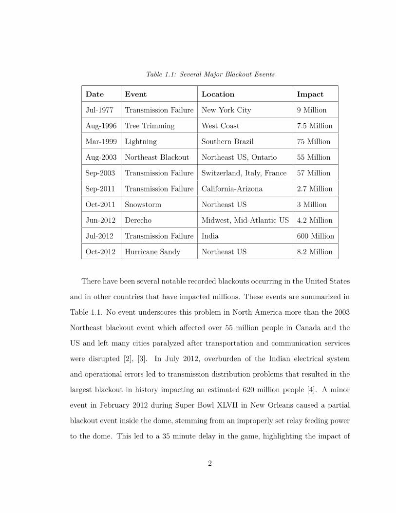
Table 1.1: Several Major Blackout Events
Date Event Location Impact
Jul-1977 Transmission Failure New York City 9 Million
Aug-1996 Tree Trimming West Coast 7.5 Million
Mar-1999 Lightning Southern Brazil 75 Million
Aug-2003 Northeast Blackout Northeast US, Ontario 55 Million
Sep-2003 Transmission Failure Switzerland, Italy, France 57 Million
Sep-2011 Transmission Failure California-Arizona 2.7 Million
Oct-2011 Snowstorm Northeast US 3 Million
Jun-2012 Derecho Midwest, Mid-Atlantic US 4.2 Million
Jul-2012 Transmission Failure India 600 Million
Oct-2012 Hurricane Sandy Northeast US 8.2 Million
There have been several notable recorded blackouts occurring in the United States
and in other countries that have impacted millions. These events are summarized in
Table 1.1. No event underscores this problem in North America more than the 2003
Northeast blackout event which affected over 55 million people in Canada and the
US and left many cities paralyzed after transportation and communication services
were disrupted [2], [3]. In July 2012, overburden of the Indian electrical system
and operational errors led to transmission distribution problems that resulted in the
largest blackout in history impacting an estimated 620 million people [4]. A minor
event in February 2012 during Super Bowl XLVII in New Orleans caused a partial
blackout event inside the dome, stemming from an improperly set relay feeding power
to the dome. This led to a 35 minute delay in the game, highlighting the impact of
2
the event to over a billion confused viewers.
An analysis of the power disruption trends is necessary to guide policymakers and
utilities to invest in building a next generation power grid, and to guide engineers
toward designs that make the grid more resilient to blackout events.
1.2 Research Questions
Summarizing power outage events helps us examine questions such as whether power
outage events are decreasing in number because smart grid funding in the United
States is increasing.1Funding of smart grid assets from government grants has been
roughly $6 billion2 with money spent on installing and deploying assets that are
supposedly increasing the reliability of our electric system. Studies into power outages
tend to focus on large individual events because they generate a large amount of
discomfort to the public and media coverage. This focus is useful in determining point
of cause and root-causes in the specific events, but may conceal other underlying
problems that are affecting the grid. Some of these problems include equipment
failure, weather vulnerabilities, operator error, and infrastructure failure. Examining
trends over time will allow us to understand crucial trends such as the frequency of
blackouts, magnitude, time of year, time of day and the geographic location of the
events. These questions can be answered using data from the Department of Energy
Office of Electricity Delivery and Energy Reliability.1This thesis only focuses on Electrical Disturbance and Reliability Event data from United States
based utilities.2In 2007 support for the smart grid became federal policy with the passage of the Energy In-
dependence and Security Act of 2007. One hundred million dollars per fiscal year was allocatedto build smart grid capabilities, and further support was provided in the American Recovery andReinvestment Act of 2009.
3
We will examine Power Outage Data from 2002-2013 provided by the DOE and
explore trends of duration, magnitude, and location. We will also explore State Re-
liability Utility Trends and attempt to determine a correlation between utilities and
states and reliability rates and smart grid investments. We will then provide recom-
mendations to utilities, and to state and federal regulatory bodies to use resources
more appropriately and enable researchers to analyze smart grid data.
Electrical Disturbance Event Hypotheses:
1. The number of power outage events is decreasing over time.
2. The loss magntiude in MW by year is decreasing over time.
3. The duration of power outage events is decreasing over time.
4. There is a relationship between the number of customers and the magnitude of
a power outage event.
5. There is a relationship between power outage duration and the magnitude of
the event.
6. The magnitude of power outage events fits a power-law distribution.
7. The number of power outage events is greater during specific times of day.
8. Some types of power outage events are more likely to occur during specific
seasons.
9. Blackout events larger than 5000 MW are rare.
Reliability Event Hypotheses:
4
10. SAIFI (Reliability Index for the frequency of outage events) values vary from
state-to-state
11. CAIDI (Reliability Index for the duration of outage events) values vary from
state-to-state
12. The frequency of power outage events is decreasing with the deployment of
smart grid assets.
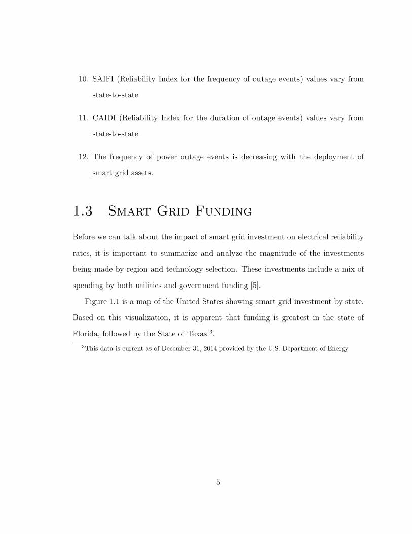
1.3 Smart Grid Funding
Before we can talk about the impact of smart grid investment on electrical reliability
rates, it is important to summarize and analyze the magnitude of the investments
being made by region and technology selection. These investments include a mix of
spending by both utilities and government funding [5].
Figure 1.1 is a map of the United States showing smart grid investment by state.
Based on this visualization, it is apparent that funding is greatest in the state of
Florida, followed by the State of Texas 3.3This data is current as of December 31, 2014 provided by the U.S. Department of Energy
5
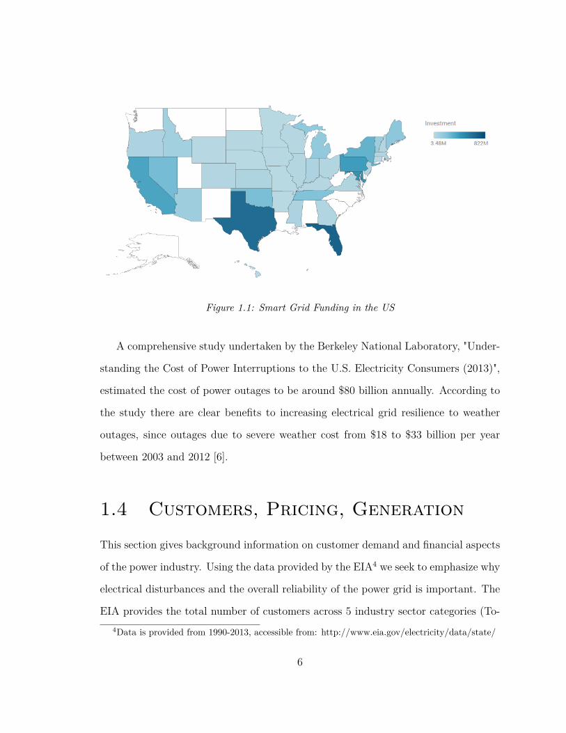
Figure 1.1: Smart Grid Funding in the US
A comprehensive study undertaken by the Berkeley National Laboratory, "Under-
standing the Cost of Power Interruptions to the U.S. Electricity Consumers (2013)",
estimated the cost of power outages to be around $80 billion annually. According to
the study there are clear benefits to increasing electrical grid resilience to weather
outages, since outages due to severe weather cost from $18 to $33 billion per year
between 2003 and 2012 [6].
1.4 Customers, Pricing, Generation
This section gives background information on customer demand and financial aspects
of the power industry. Using the data provided by the EIA4 we seek to emphasize why
electrical disturbances and the overall reliability of the power grid is important. The
EIA provides the total number of customers across 5 industry sector categories (To-4Data is provided from 1990-2013, accessible from: http://www.eia.gov/electricity/data/state/
6
tal Electric Industry, Full-Service Providers, Restructured Retail Service Providers,
Energy-Only Providers, and Delivery-Only Service). The number of customer ref-
erenced in Figure 1.2 is the Total Electric Industry value. The population of the
United States has increased from 250 to 309.3 million as measured by the 2000 and
2010 census. We expect therefore, that the number of customers and consequentially
the generation capacity should increase. Consequently, we list these out as assertions
to motivate why it is important to understand electrical disturbances and reliability.
1.5 Assertions
1.5.1 Assertion 1
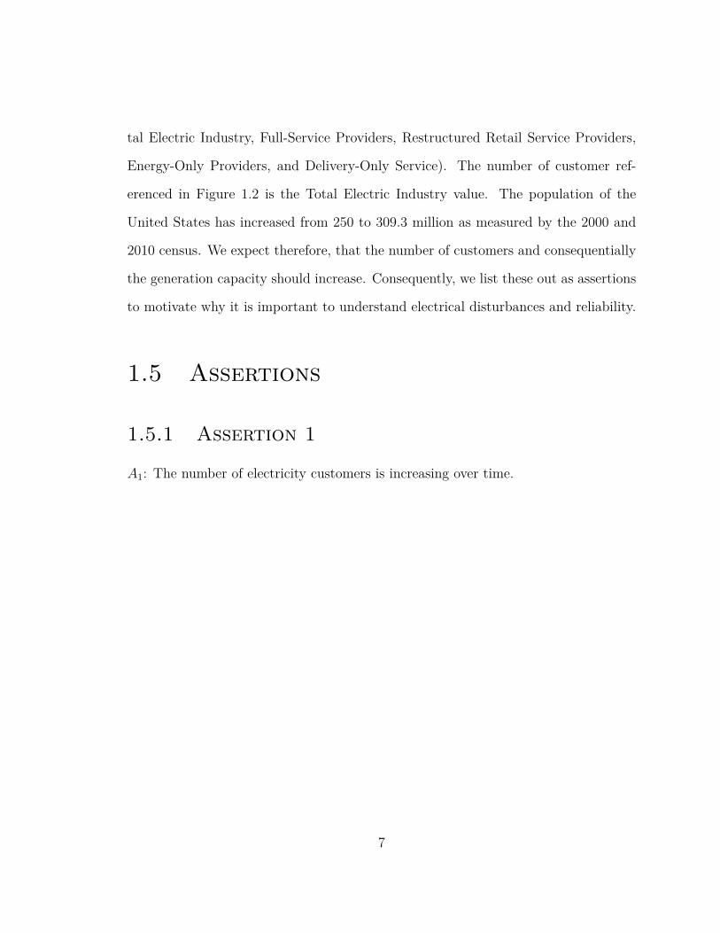
A1: The number of electricity customers is increasing over time.
7
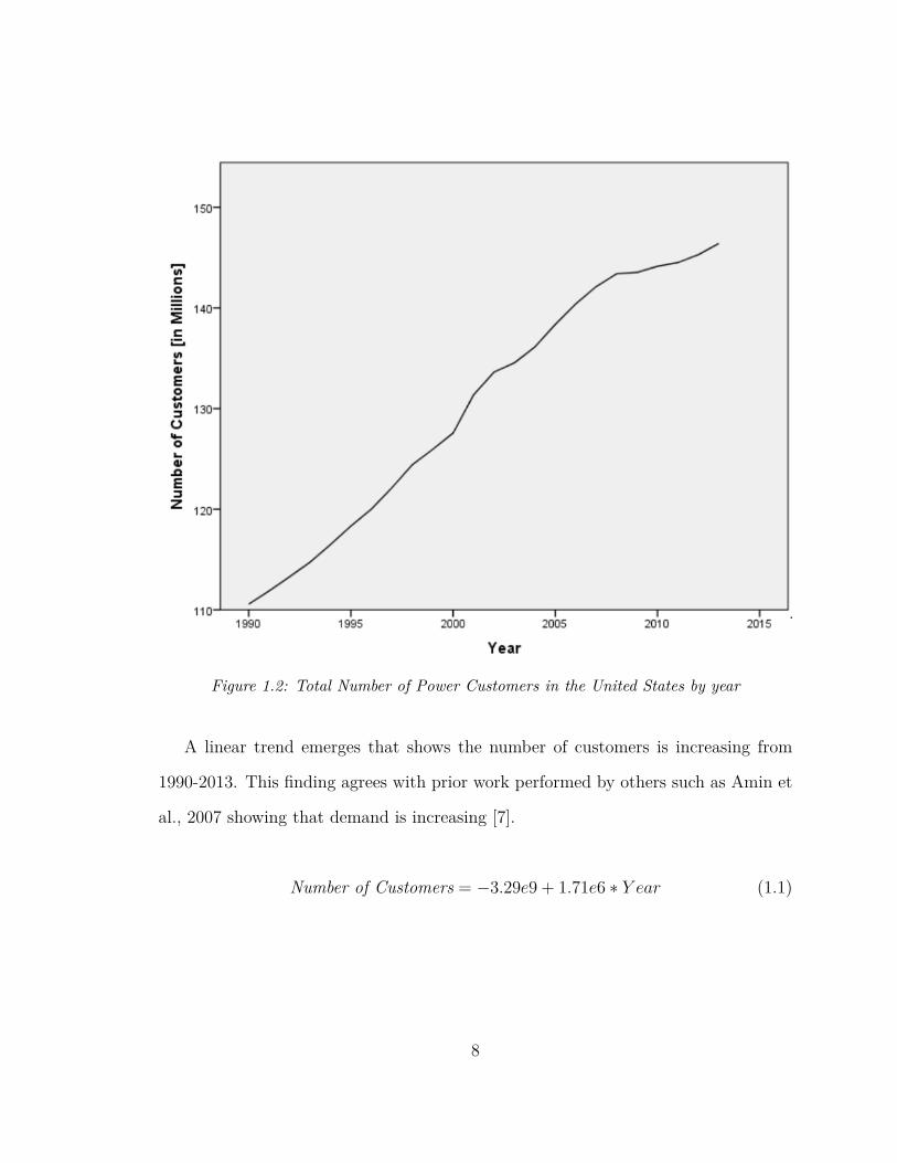
Figure 1.2: Total Number of Power Customers in the United States by year
A linear trend emerges that shows the number of customers is increasing from
1990-2013. This finding agrees with prior work performed by others such as Amin et
al., 2007 showing that demand is increasing [7].
Number of Customers = −3.29e9 + 1.71e6 ∗ Y ear (1.1)
8
1.5.2 Assertion 2
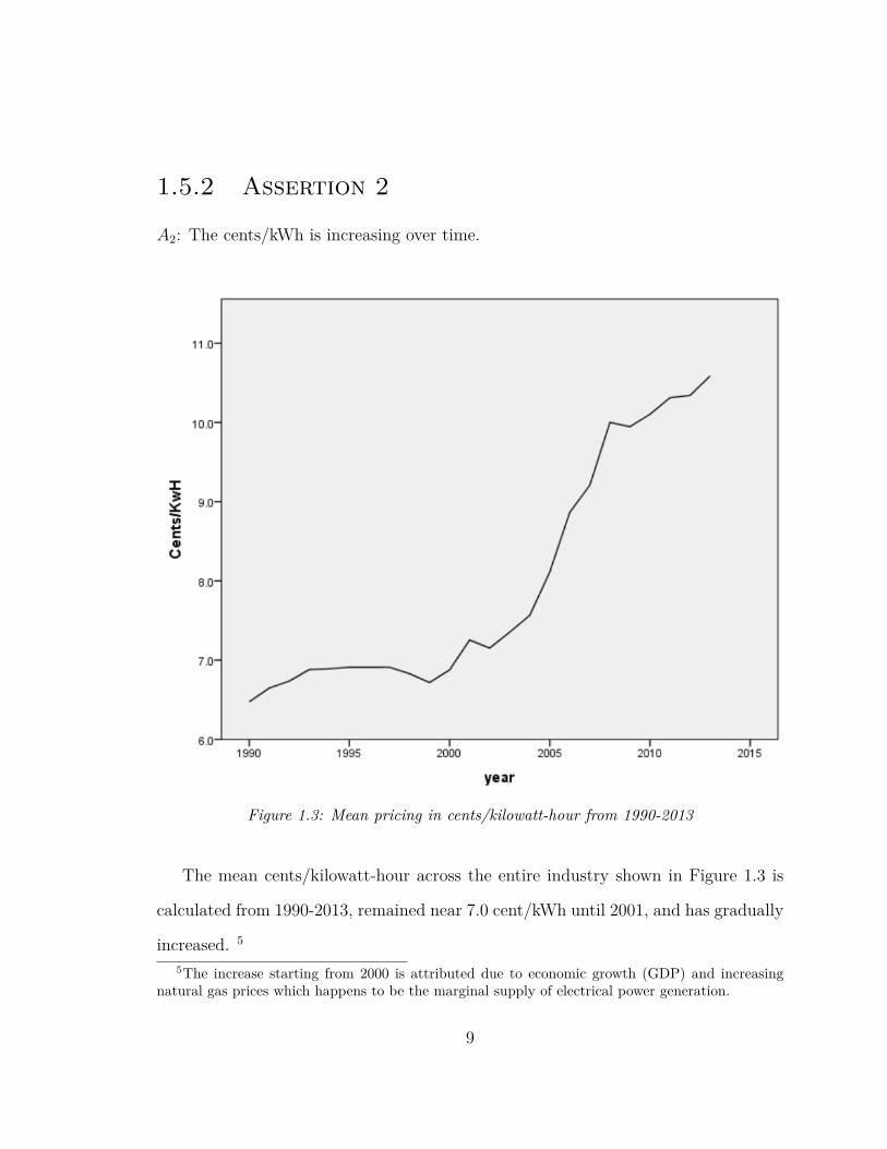
A2: The cents/kWh is increasing over time.
Figure 1.3: Mean pricing in cents/kilowatt-hour from 1990-2013
The mean cents/kilowatt-hour across the entire industry shown in Figure 1.3 is
calculated from 1990-2013, remained near 7.0 cent/kWh until 2001, and has gradually
increased. 5
5The increase starting from 2000 is attributed due to economic growth (GDP) and increasingnatural gas prices which happens to be the marginal supply of electrical power generation.
9
Cost = −3.73e2 + 0.19 ∗ Y ear + 1.12e− 2 ∗ (Y ear − 2001.5)2 (1.2)
1.5.3 Assertion 3
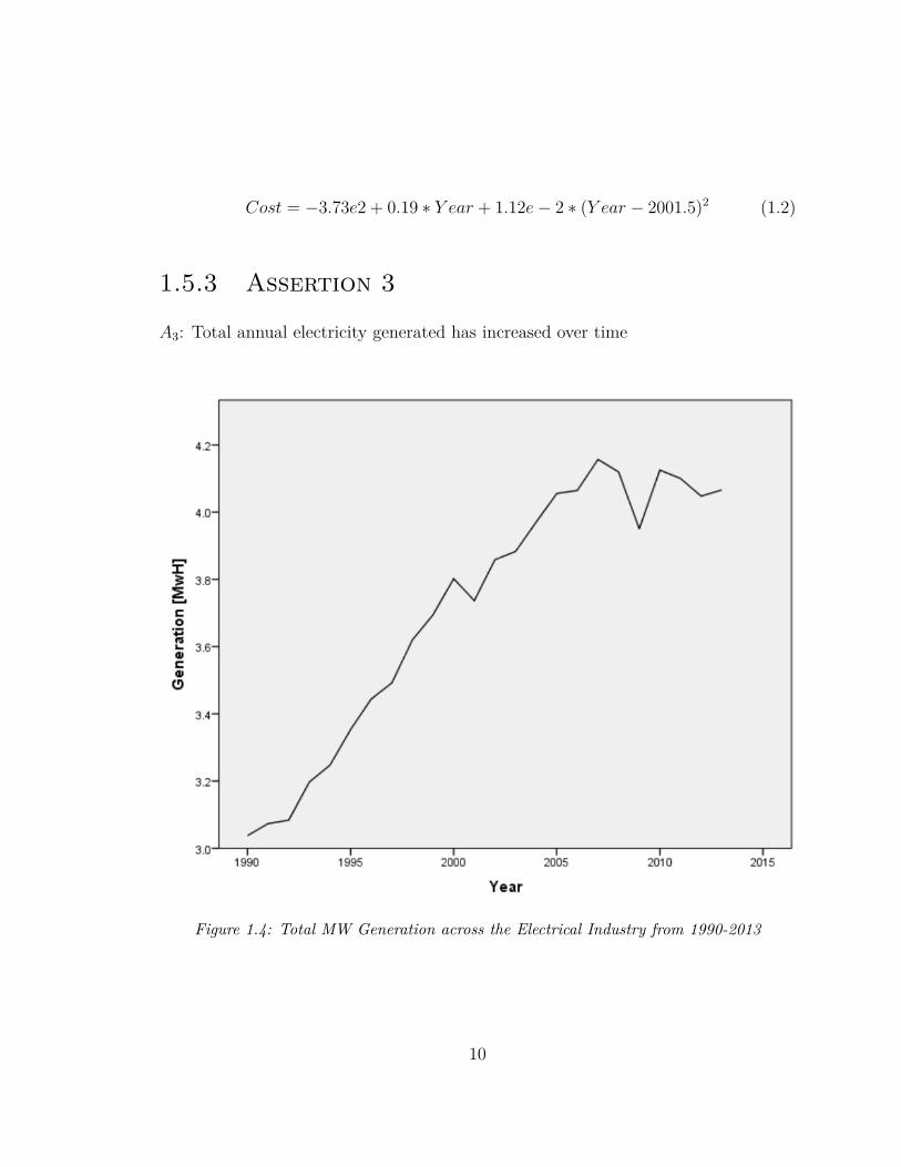
A3: Total annual electricity generated has increased over time
Figure 1.4: Total MW Generation across the Electrical Industry from 1990-2013
10
Generation MegaWattHours = −9.84e10 + 5.11e7 ∗ Y ear− 2.46e6 ∗ (Y ear− 2001.5)2
(1.3)
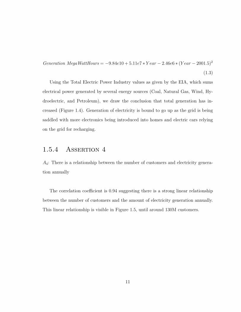
Using the Total Electric Power Industry values as given by the EIA, which sums
electrical power generated by several energy sources (Coal, Natural Gas, Wind, Hy-
droelectric, and Petroleum), we draw the conclusion that total generation has in-
creased (Figure 1.4). Generation of electricity is bound to go up as the grid is being
saddled with more electronics being introduced into homes and electric cars relying
on the grid for recharging.
1.5.4 Assertion 4
A4: There is a relationship between the number of customers and electricity genera-
tion annually
The correlation coefficient is 0.94 suggesting there is a strong linear relationship
between the number of customers and the amount of electricity generation annually.
This linear relationship is visible in Figure 1.5, until around 130M customers.
11
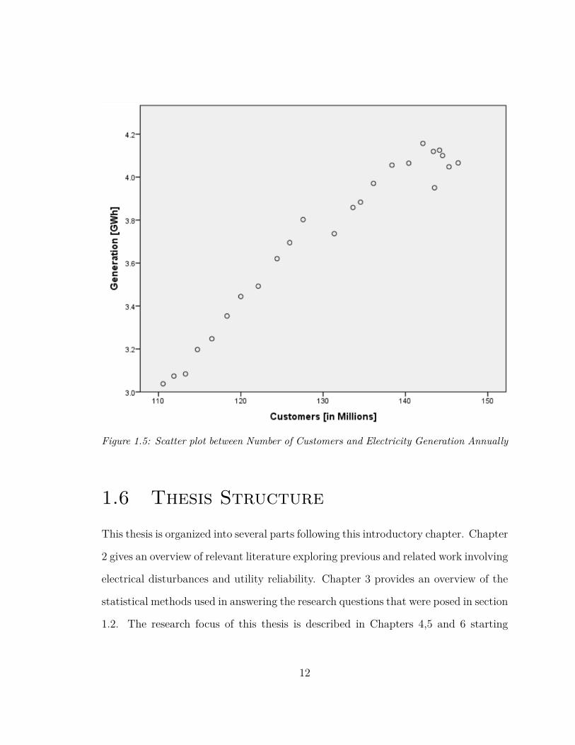
Figure 1.5: Scatter plot between Number of Customers and Electricity Generation Annually
1.6 Thesis Structure
This thesis is organized into several parts following this introductory chapter. Chapter
2 gives an overview of relevant literature exploring previous and related work involving
electrical disturbances and utility reliability. Chapter 3 provides an overview of the
statistical methods used in answering the research questions that were posed in section
1.2. The research focus of this thesis is described in Chapters 4,5 and 6 starting
12
with an exploration of electrical disturbance data, followed by reliability data, and
concluded with a summary of recommendations and future work.
13
Chapter 2
Literature Review
A significant number of publications from research organizations, governmental bod-
ies, and utilities have focused on understanding the causes of power outages, and
providing analysis of those events. Several articles provide trends of blackout data,
weather trends, and discussions of the age of the infrastructure and need for invest-
ment in the grid. There are also a number of white papers and fact sheets from
special interest organizations that extol the benefits of the smart gird. In this sec-
tion, we will provide an overview of previously published work and discuss research
questions that have been posed. It is also our goal to detect gaps in current research
work. In addition, the literature review should clarify why we are choosing to focus
on the research questions posed in the introduction. The review also helps the reader
understand why answering questions related to electrical disturbance, reliability, and
smart grid funding is important. We want the reader to take away why our research
is new compared to previous approaches.
14
2.1 Blackout Trends and Reliability
The most relevant and well cited article on this topic, Hines, et al., "Large Blackouts
in North America Historical Trends and Policy Implications", summarized blackout
trends in North America using NERC Data from 1984-2006 [8]. They conclude that
the frequency of large scale blackouts is not decreasing. They have shown that these
trends hold even after adjusting for elevated demand and increased population. The
authors did not find a correlation between blackout sizes and blackout duration.
Considering that the trends were examined from 1984-2006, it is worth examining
more recent data to further extend their work.
A study, "An Examination of Temporal Trends in Electricity Reliability Based on
Reports from U.S. Electric Utilities", conducted by the Lawrence Berkeley National
Lab [9] found that power interruptions have increased at a rate of about 2 percent per
year over a period of over 10 years, using utility reliability data obtained from state
regulatory bodies. The study drew the conclusion that reliability data trends are
not improving because smart grid technology such as automated outage management
systems is reporting service interruptions more accurately. The authors make it clear
that since their findings are based on a sample of reliability data from several utilities,
they do not attempt to make claims about overall power reliability in the US.
One thing we are very interested in is looking at is the implementation of smart
grid assets such as smart meters and their impact on reliability at several utilities.
With our study we will also use a "convenience sample" based on information that is
already available.
15
2.2 Weather Trends
A report by Climate Central, (Kenward et al.) analyzed power outage data over
a 28 year period using a combination of reporting from the DOE and NERC [10].
Summarized in the report, it is pointed out that between 2003-2012 80% of all outages
were caused by weather. 1 The authors’ data shows a clear trend of weather related
incidents, but the authors highlight the fact that physical attacks, and cyber attacks
have also increased on the power grid and should be reported. Campbell et al., 2012,
of the Congressional Research Service, highlights the damage to the electrical grid
caused by seasonal storms, rain, and high winds. These weather events lead to trees
failing on local distribution and transmission lines causing power outages.
2.3 Infrastructure
Amin et al., 2003, show the impact of infrastructure on grid reliability. They cite
several reasons why grid reliability has decreased, but the primary reason is that the
grid relies on technology that was developed in the mid-20th century. Due to the
age of the infrastructure and without a methodical plan to take into account growing
demands on the grid from the digital era, the grid is not very reliable. They argue
that investment in technologies made by utilities, independent regional transmission
operations, and funding from the government will improve the overall reliability of
the electrical grid, and make the grid more resilient to natural disasters and secure
to terrorist attacks. I would like to test the assertion that investment in smart grid1We will use our DOE data from 2002-2014 to see if we reach a similar conclusion.
16
technologies is improving overall reliability.
2.4 Smart Grid Deployment
Farhangi et al., 2010, explain some of the most commonly touted advantages of the
smart grid, including the ability to better predict demand with a network of smart
meters. Distribution automation, substation automation, and IT infrastructure to
provide real-time feedback, control and monitoring of transmission and distribution
systems.
There are a number of government white papers that have been published cat-
aloging the progress made by utilities that have received funding from the federal
government. For instance, the Smart Grid Investment Grant Program (run by the
DOE), published a progress report in October 2013, that highlights reliability im-
provements observed through decreasing reliability indices (CAIDI,SAIFI, etc). The
report pointed out that projects using automated feeder switching were able to re-
duce the frequency of outages. No statistics were shown in the report to make the
correlation between reliability indices and spending.
2.5 Spending
An Associated Press (AP) article by Fahey 2013 et al. [11] detailing an analysis of
utility spending and reliability concluded that consumers are spending more money on
their utility bill while power loss duration has increased. In the conclusion reached
by the AP analysis, they believe that utilities are misspending the money or not
17
spending enough money.
The article makes a few good points, including that power reliability steadily
increased from the 1950s to the middle of the 1990s as automatic switches were
installed that prevented small failures from becoming cascading failures. Accordingly,
(argued by the authors) given that reliability rates leveled off, utilities and regulators
diverted their attention. Overall spending has increased in the past decade. It is
worth examining some of the claims made by the article, in particular, the fact that
there has been a 15% increase in outage duration time.
In this analysis, they compared reliability statistics with spending across 210 util-
ities and across 24 categories of local distribution equipment. This article raises the
question of how to correlate spending on smart grid to improvements in reliability.
This is exactly one question that we are seeking to answer. They do not provide an
overview of the statistical methods used in their article. While there is no reason to
believe the article is biased or incorrect, we should investigate these assertions as a
third party with no agenda in mind.
2.6 Cascading Blackout Trends
Dobson et al., 2006, stipulates that large blackouts are rare and unpredictable, and, as
a result are hard to analyze and simulate. Calculating the risk of blackouts of all sizes
can be accomplished by using data collected from regulatory bodies that include MW,
restoration time, and the number of customers. From this data, Dobson estimates the
probability distribution of blackout sizes. It is verified by the work of several authors
(Dobson et al., 2006, Hines et al. 2009, etc) that large blackouts follow a power law
18
distribution [12].
2.7 Claims made by Fact sheets
The claims made by fact sheets from utilities, special interest groups, and government
organizations are almost endless on advantages of the smart grid, and tout the benefits
to the consumers.
A fact sheet released by the White House in 2011, states that not much has
changed in the electric grid since Edison brought the first electric grid into operation.
The administration points out that $4.5 billion of the American Recovery and Invest-
ment Act (also known as the Stimulus Bill) has been allocated towards modernizing
American aging infrastructure. A fact sheet produced by the Energy Defense Fund,
a special interest group, argues that the smart grid will provide more reliable service
through shorter and fewer outages.
The Smart Grid Consumer Collaborative published in 2011 that the smart grid
technologies will overhaul aging equipment and reduce the number of blackouts by
enabling the grid to meet increasing demand. Reduced cost to both the end-customer
and the utility is claimed. We are interested in being able to perform a return-
on-investment analysis for utilities on smart grid technologies to determine whether
spending on the technological upgrades produce a positive return in investment.
19
Chapter 3
Methods
The goal of this chapter is to provide an overview of the statistical methods used
in this thesis to answer the underlying research questions listed in the introduction.
We don’t know whether the data is normally or non-normally distributed. This is
important to determine so we know whether to use parametric or non-parametric
techniques, respectively.
Many of the research questions involve determining whether certain trends ex-
ist, such as if power outage events are decreasing over time. Regression techniques
(ANOVA, Possion) and time series models (ARMA) are favored when looked for
trends over a period of time.
In addition to regression techniques, pre-and-post analysis of the number of power
outage events grouped pre-2008, post-2008, would need to be assessed using a com-
parison technique such as Kolmogorov-Smirnov or Kruskal-Wallis evaluating whether
the median differs between two populations.
An overview of the statistical methods used in this thesis to analyze data is re-
viewed in this chapter.
20
3.1 Testing for Normality
In order to determine whether it is appropriate to use parametric tests to analyze our
dataset we must determine if the data are normal or not [13]. There are a number of
ways to do this. A simple plot of the data may yield information showing the data is
skewed. The properties of a normal (or Gaussian) distribution include:
• Continuous and symmetrical with both tails extending to infinity
• Arithmetic mean, mode, median are identical
• Shape of the curve is determined by the mean and standard deviation
The normal distribution is given by:
F (x, u, σ) = 1σ√
2πe−
(x− µ)2σ2
2
(3.1)
µ is defined as the mean or expectation of the distribution. σ is the standard
deviation
3.2 Spearman’s rank correlation coef-
ficient
Often researchers are interested in determining the relationship between two variables.
We do not know the underlying distribution of the data and there is evidence it is not
normally distributed. Thus we rely on non-parametric methods to determine if there
21
is a statistical dependence between the two variables. It assesses if the relationship
between the two variables can be described using a monotonic function.
The Spearman correlation coefficient is defined as the Pearson correlation coeffi-
cient between the ranked variables. For a sample size of n, the n raw scores Xi, Yi
are converted to ranks to xi, yi and ρ is computed from Eq. 3.2, and di = xi − yi is
the difference between ranks.
ρ = 1− 6 ∑ ∗d2i
n(n2 − 1) (3.2)
The coefficient is interpreted such that the sign of the Spearman correlation indi-
cates the direction of the association between X(the independent variable) and Y(the
dependent variable). The Spearman correlation coefficient is positive is Y tends to
increase when X increases, and negative when Y tends to decrease when X increases.
3.3 Power Law Distribution
A power law, in statistical terms describes a functional relationship between two
quantities, such that one quantity varies as a power of another. A variety of things fit a
power law distribution including physical, biological, and man-made phenomena [14].
It has been found that the size of power outages follow a power law distribution.
p(x) ∝ x−α (3.3)
A quantity x is drawn from a probability distribution (X), with ∝ (referred to as
the scaling or exponent parameter). This parameter typically ranges between 2 and
22
3. A continuous power-law distribution is described by p(x):
p(x)dx = Pr(x ≤ X < x+ dx) = Ax−αdx (3.4)
where X is the observed value and A is the normalization constant. We see that
the density diverges as x −→ 0. Noticing the equation cannot hold for α ≥ 0, we must
generate a lower bound to the power-law behavior. This bound can be denoted xmin
leading to equation 3.4, if α > 1, we calculate a normalizing constant and generate
the following equation.
p(x) = α− 1xmin
( x
xmin)−α (3.5)
Fitting the power law to empirical data, requires estimating the scaling parameter
α, that also requires calculating the xmin value. If the value is unknown we can
calculate this from the dataset. Assuming our data follows a power law distribution
for xi >≥ xmin, the α can be calculated using: 1 + n, where n are the observed values
of x.
Using the Kolmogorov-Smirnov or KS statistic, where we can find xmin, that
minimizes D, where D = max | F(x) - S(x) |, and where we define S(x) as the empirical
distribution function, and F(x) as the specified hypothetical distribution function.
Thus we can summarize the fitting procedure as:
1. xmin is estimated using maximum likelihood and we calculate the KS good-of-fit
statistic D
2. Using our estimate of x-min, we chose the minimum value of D over all values
of xmin
23
In the next section we will discuss the KS statistic.
3.4 Kolmogorov-Smirnov
When it is not known whether the underlying distribution is normally distributed
or if is determined not to be so, we rely on non-parametric methods just like the
Spearman correlation coefficient previously discussed. The Kolmogorov-Smirnov test
can be used to compare a sample with a reference probability distribution referred
to as a (one-sample KS test), or used to compare two samples with each other a
(two-sample KS test). The KS statistic quantifies the distance between the empirical
distribution function of the sample and the cumulative distribution function of the
reference function. The Kolmogorov-Smirnov test is defined by the following:
Ho: The data follow a specified distribution
Ha: The data do not follow the specified distribution
For two-sample testing, the KS test is preferred because it is sensitive to differences
in both location and shape of the empirical cumulative distribution function of the
two samples. In the two-sample case, the KS statistic is, where n is the items :
D = supx|F1,n(x)− F2,n′(x)| (3.6)
where F1,n and F2,n′ are the empirical distribution functions of the first and second
sample, n and n’ are the observation numbers for the sampling corresponding to F1,n
and F2,n′ , and sup is the supremum function. The null hypothesis is rejected at level
noted in table 3.1. If
24
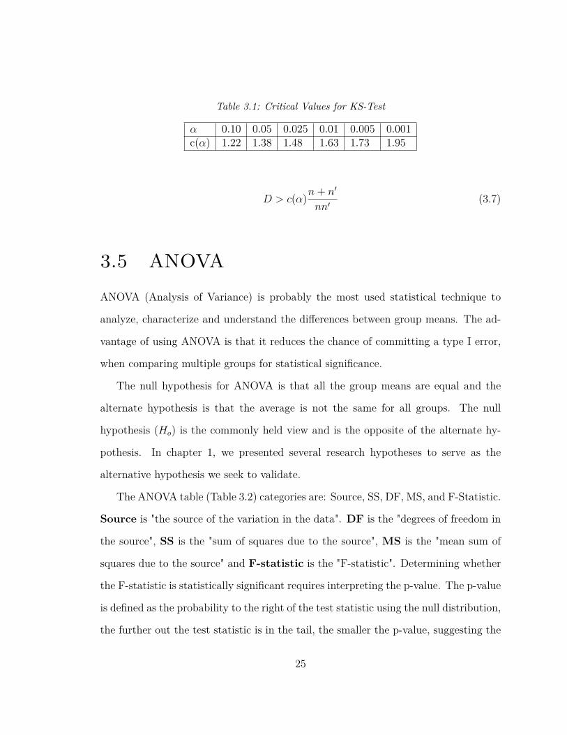
Table 3.1: Critical Values for KS-Test
α 0.10 0.05 0.025 0.01 0.005 0.001c(α) 1.22 1.38 1.48 1.63 1.73 1.95
D > c(α)n+ n′
nn′(3.7)
3.5 ANOVA
ANOVA (Analysis of Variance) is probably the most used statistical technique to
analyze, characterize and understand the differences between group means. The ad-
vantage of using ANOVA is that it reduces the chance of committing a type I error,
when comparing multiple groups for statistical significance.
The null hypothesis for ANOVA is that all the group means are equal and the
alternate hypothesis is that the average is not the same for all groups. The null
hypothesis (Ho) is the commonly held view and is the opposite of the alternate hy-
pothesis. In chapter 1, we presented several research hypotheses to serve as the
alternative hypothesis we seek to validate.
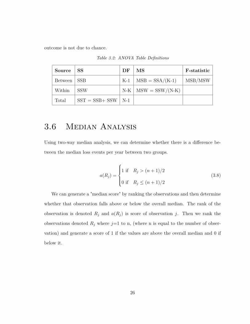
The ANOVA table (Table 3.2) categories are: Source, SS, DF, MS, and F-Statistic.
Source is "the source of the variation in the data". DF is the "degrees of freedom in
the source", SS is the "sum of squares due to the source", MS is the "mean sum of
squares due to the source" and F-statistic is the "F-statistic". Determining whether
the F-statistic is statistically significant requires interpreting the p-value. The p-value
is defined as the probability to the right of the test statistic using the null distribution,
the further out the test statistic is in the tail, the smaller the p-value, suggesting the
25
outcome is not due to chance.
Table 3.2: ANOVA Table Definitions
Source SS DF MS F-statistic
Between SSB K-1 MSB = SSA/(K-1) MSB/MSW
Within SSW N-K MSW = SSW/(N-K)
Total SST = SSB+ SSW N-1
3.6 Median Analysis
Using two-way median analysis, we can determine whether there is a difference be-
tween the median loss events per year between two groups.
a(Rj) =
1 if Rj > (n+ 1)/2
0 if Rj ≤ (n+ 1)/2(3.8)
We can generate a "median score" by ranking the observations and then determine
whether that observation falls above or below the overall median. The rank of the
observation is denoted Rj and a(Rj) is score of observation j. Then we rank the
observations denoted Rj where j=1 to n, (where n is equal to the number of obser-
vation) and generate a score of 1 if the values are above the overall median and 0 if
below it.
26
3.7 Analysis of Means Methods
The analysis of means (ANOM) methods compare means and variances and other
measures of location and scale across several groups. It can be used to test whether
any of the group means are statistically different from the overall (sample) mean. It
can also be used to test whether any of the group ranges are statistically different
from the overall mean of the ranges. An analysis of means chart can be used to
determine whether there is a statistical difference between a group’s statistic and the
overall average of the statistics for all the groups.
3.8 Model Building
3.8.1 Generalized Linear Model
A generalized linear model (GLM) is an ordinary linear regression that allows for
response variables that fit error distribution models other than the normal distribu-
tions.
g(µm) = β0 + β1X1 + ...+ βmXm (3.9)
where m = variable of interest, β0 = intercept, β1 = coefficient for X1, X1 =
independent variable 1.
27
3.8.2 Poisson Regression Model
Poisson regression is used for modeling count variables. The result is a generalized
linear model with Poisson response and log link. The Poisson Distribution is as
follows: A Random Variable (Z) has a Poisson distribution with parameter µ if it
takes a integer z = 0,1,2...with probability:
Pr(Z = z) = e−µµz
z! (3.10)
with expected value and variance, defined by
E(Z) = var(Z) = µ. (3.11)
We can model a Poisson regression by using equation 3.12.
log(Counts) = Intercept+ b1X1 + b2X2 + bmXm (3.12)
3.8.3 ARMA
Autoregressive-moving average (ARMA) models provide a stationary stochastic pro-
cess in terms of two polynomials, one for auto-regression and the second for the
moving average. There are two parts of the ARMA(p,q) model, where p is the or-
der of the autoregressive part and q is the order of the moving average part. The
autoregressive processes have in general, infinite non-zero autocorrelation coefficients
that decay with the lag. The AR processes have a relatively long memory, since the
current value of a series is correlated with all previous ones, although with decreasing
28
coefficients.
ARMA(1, 1) = Xt − φXt−1 = Zt + θ ∗ Zt−1 (3.13)
Hence, when φ = 0 then ARMA(1,1) = MA(1), Movingaverage(1), and we denote
such a process as ARMA(0,1). Similarly, when θ = 0 then ARMA(1,1) = AR(1),
Autoregressive(1), and we denote such process as ARMA(1,0).
3.8.4 Spline
A spline is numerical fuction that is piecewise-defined by polynomial functions and
maintains a high degree of smoothness.
3.8.5 Software Package
Several statistical software packages are used to perform analysis including JMP, R,
SAS and SPSS.
29
Chapter 4
Understanding Electrical Distur-
bances Events
4.1 Introduction
Electrical Disturbance Events are reported on form (OE-417) by the Department of
Energy (DOE). This is the information we chose for statistical analysis. As discussed
in the introduction, OE-417 must be filled out by electric utilities and reliability
authorities when an electrical disturbance exceeds the reporting threshold. A copy
of the form is attached in the appendix. Form OE-417 is approved for use by all 50
states, the District of Columbia, Puerto Rico, the US Virgin Islands and the US Trust
Territories. Each year an annual summary is compiled in spreadsheet/PDF format
and made available on-line from the DOE website to those that are interested. A
listing and description of the variables is given in Table 4.1.
30
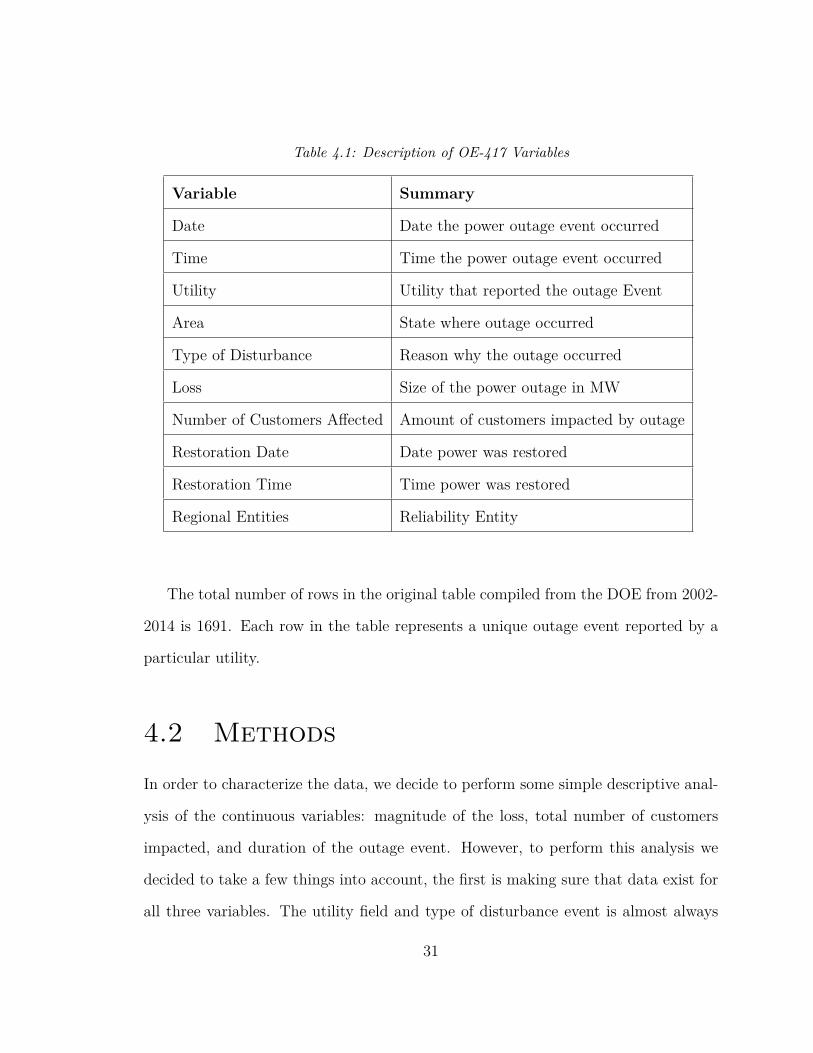
Table 4.1: Description of OE-417 Variables
Variable Summary
Date Date the power outage event occurred
Time Time the power outage event occurred
Utility Utility that reported the outage Event
Area State where outage occurred
Type of Disturbance Reason why the outage occurred
Loss Size of the power outage in MW
Number of Customers Affected Amount of customers impacted by outage
Restoration Date Date power was restored
Restoration Time Time power was restored
Regional Entities Reliability Entity
The total number of rows in the original table compiled from the DOE from 2002-
2014 is 1691. Each row in the table represents a unique outage event reported by a
particular utility.
4.2 Methods
In order to characterize the data, we decide to perform some simple descriptive anal-
ysis of the continuous variables: magnitude of the loss, total number of customers
impacted, and duration of the outage event. However, to perform this analysis we
decided to take a few things into account, the first is making sure that data exist for
all three variables. The utility field and type of disturbance event is almost always
31
filled out, however the number of customers, loss magnitude and duration is sometime
unknown. After the applying this criteria only 614 observations remained.
Distribution information was generated for several of the variables, and a variety of
visualizations created to examine trends for a variety of things we were interested in.
A frequency table was created based on the cause of outage events was generated so it
could be determined which outage events were occurring more than others. Based on
findings from previous research we expect that number of customers, loss magnitude,
and duration would be skewed so we decide to perform a logarithmic transformation
on the data. Then we use ANOVA to determine whether there are differences between
the number of customers impacted, the magnitude of the loss, and the duration of
the outage, when grouped by season, time of day, and cause of outage.
In order to determine if season has an effect we split the events using the month
they occured into the categories: Spring, Summer, Fall, and Winter. To determine
if the the time of day impacts the number of outage events we define time period as
Period1-Period4: 0-7, 7-12, 13-18, 19-24 on a 24-Hour clock.
The smart grid became federal policy with the passage of the Energy Independence
and Security Act of 2007. Passage of the act set aside $100 million in funding per
fiscal year from 2008-2012, and further supplemented that by another $4.5 billion from
the American Recovery and Reinvestment Act of 2009 for the creation of the smart
grid. Taking these facts into account while testing hypothesis statements looking for
trends over time, it makes sense to separate pre-2008, and post-2008 data to give us
an idea of whether the focus on improving the grid played a role. This splitting of the
date range makes sense as we would expect with spending in smart grid technology,
perhaps a decrease in outage event metrics would be apparent in our analysis.
32
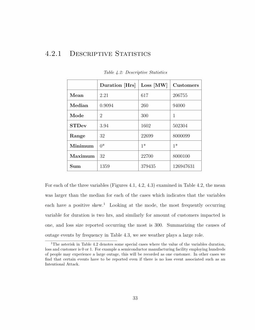
4.2.1 Descriptive Statistics
Table 4.2: Descriptive Statistics
Duration [Hrs] Loss [MW] Customers
Mean 2.21 617 206755
Median 0.9094 260 94000
Mode 2 300 1
STDev 3.94 1602 502304
Range 32 22699 8000099
Minimum 0* 1* 1*
Maximum 32 22700 8000100
Sum 1359 379435 126947631
For each of the three variables (Figures 4.1, 4.2, 4.3) examined in Table 4.2, the mean
was larger than the median for each of the cases which indicates that the variables
each have a positive skew.1 Looking at the mode, the most frequently occurring
variable for duration is two hrs, and similarly for amount of customers impacted is
one, and loss size reported occurring the most is 300. Summarizing the causes of
outage events by frequency in Table 4.3, we see weather plays a large role.1The asterisk in Table 4.2 denotes some special cases where the value of the variables duration,
loss and customer is 0 or 1. For example a semiconductor manufacturing facility employing hundredsof people may experience a large outage, this will be recorded as one customer. In other cases wefind that certain events have to be reported even if there is no loss event associated such as anIntentional Attack.
33
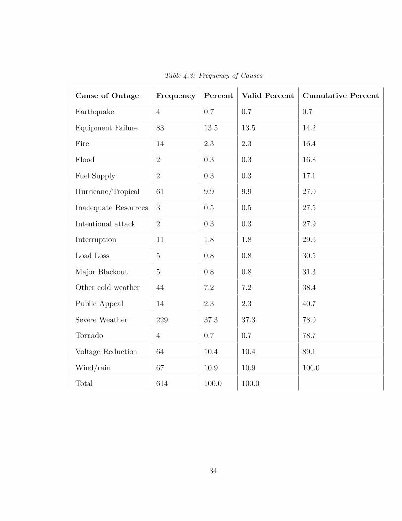
Table 4.3: Frequency of Causes
Cause of Outage Frequency Percent Valid Percent Cumulative Percent
Earthquake 4 0.7 0.7 0.7
Equipment Failure 83 13.5 13.5 14.2
Fire 14 2.3 2.3 16.4
Flood 2 0.3 0.3 16.8
Fuel Supply 2 0.3 0.3 17.1
Hurricane/Tropical 61 9.9 9.9 27.0
Inadequate Resources 3 0.5 0.5 27.5
Intentional attack 2 0.3 0.3 27.9
Interruption 11 1.8 1.8 29.6
Load Loss 5 0.8 0.8 30.5
Major Blackout 5 0.8 0.8 31.3
Other cold weather 44 7.2 7.2 38.4
Public Appeal 14 2.3 2.3 40.7
Severe Weather 229 37.3 37.3 78.0
Tornado 4 0.7 0.7 78.7
Voltage Reduction 64 10.4 10.4 89.1
Wind/rain 67 10.9 10.9 100.0
Total 614 100.0 100.0
34
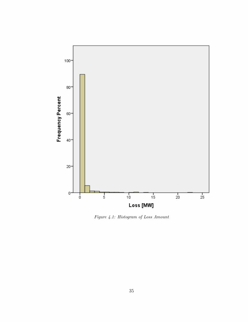
Figure 4.1: Histogram of Loss Amount
35
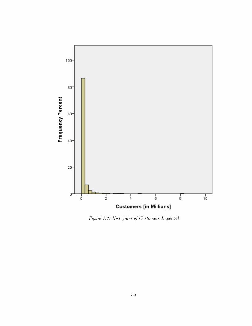
Figure 4.2: Histogram of Customers Impacted
36
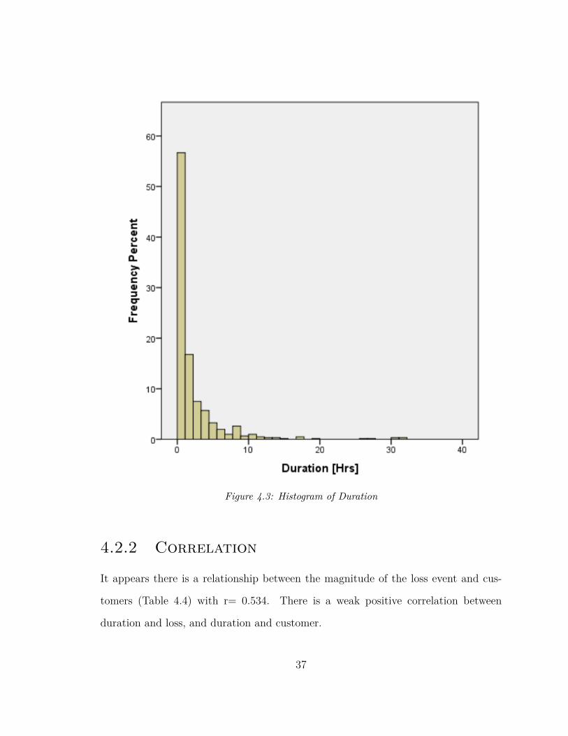
Figure 4.3: Histogram of Duration
4.2.2 Correlation
It appears there is a relationship between the magnitude of the loss event and cus-
tomers (Table 4.4) with r= 0.534. There is a weak positive correlation between
duration and loss, and duration and customer.
37
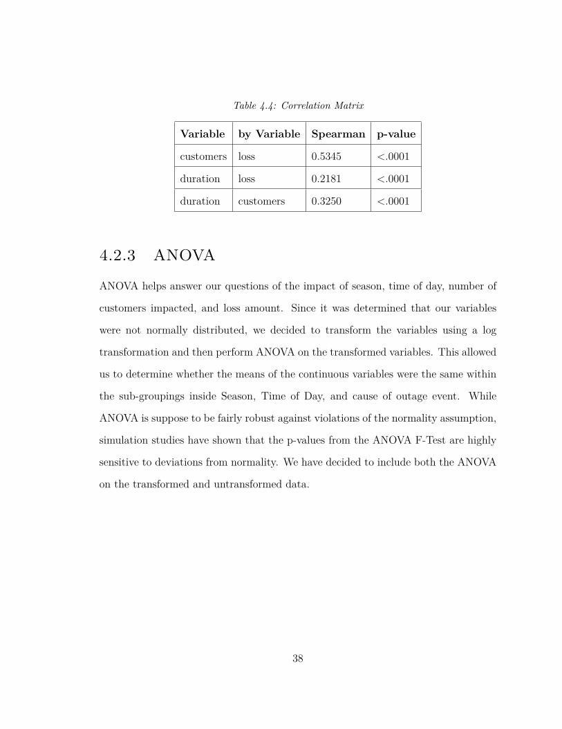
Table 4.4: Correlation Matrix
Variable by Variable Spearman p-value
customers loss 0.5345 <.0001
duration loss 0.2181 <.0001
duration customers 0.3250 <.0001
4.2.3 ANOVA
ANOVA helps answer our questions of the impact of season, time of day, number of
customers impacted, and loss amount. Since it was determined that our variables
were not normally distributed, we decided to transform the variables using a log
transformation and then perform ANOVA on the transformed variables. This allowed
us to determine whether the means of the continuous variables were the same within
the sub-groupings inside Season, Time of Day, and cause of outage event. While
ANOVA is suppose to be fairly robust against violations of the normality assumption,
simulation studies have shown that the p-values from the ANOVA F-Test are highly
sensitive to deviations from normality. We have decided to include both the ANOVA
on the transformed and untransformed data.
38

Table 4.5: ANOVA table where group = Cause of Outage
Variable Sum of Squares df Mean Square F Sig.
loss Between Groups 197412174 16 12338260 5.35 .000
Within Groups 1376817084 597 2306226
Total 1574229259 613
duration Between Groups 1836 16 114 8.890 .000
Within Groups 7708.937 597 12.913
Total 9545.671 613
customers Between Groups 16347198005664 16 1021699875354 4.410 .000
Within Groups 138318879942262 597 231689916151
Total 154666077947927 613
log_loss Between Groups 206 16 12.90 7.78 .000
Within Groups 989 597 1.65
Total 1196 613
log_duration Between Groups 911 16 56.95 21.61 .000
Within Groups 1572 597 2.635
Total 2484 613
log_customers Between Groups 1033 16 64.60 11.752 .000
Within Groups 3282 597 5.498
Total 4315 613
39
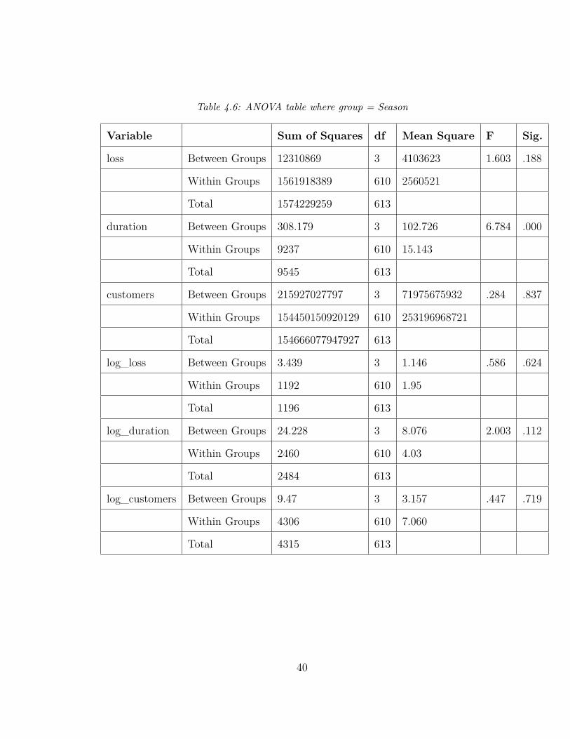
Table 4.6: ANOVA table where group = Season
Variable Sum of Squares df Mean Square F Sig.
loss Between Groups 12310869 3 4103623 1.603 .188
Within Groups 1561918389 610 2560521
Total 1574229259 613
duration Between Groups 308.179 3 102.726 6.784 .000
Within Groups 9237 610 15.143
Total 9545 613
customers Between Groups 215927027797 3 71975675932 .284 .837
Within Groups 154450150920129 610 253196968721
Total 154666077947927 613
log_loss Between Groups 3.439 3 1.146 .586 .624
Within Groups 1192 610 1.95
Total 1196 613
log_duration Between Groups 24.228 3 8.076 2.003 .112
Within Groups 2460 610 4.03
Total 2484 613
log_customers Between Groups 9.47 3 3.157 .447 .719
Within Groups 4306 610 7.060
Total 4315 613
40
Table 4.7: ANOVA table where group = Time of Day
Variable Sum of Squares df Mean Square F Sig.
loss Between Groups 8302800 3 2767600 1.078 .358
Within Groups 1565926458 610 2567092
Total 1574229259 613
duration Between Groups 5.517 3 1.839 .118 .950
Within Groups 9540 610 15.640
Total 9545 613
customers Between Groups 169064084240 3 56354694746 .223 .881
Within Groups 154497013863686 610 253273793219
Total 154666077947927 613
log_loss Between Groups 5.73 3 1.91 .979 .402
Within Groups 1190 610 1.95
Total 1196 613
log_duration Between Groups 64.81 3 21.60 5.447 .001
Within Groups 2419 610 3.966
Total 2484 613
log_customers Between Groups 4.953 3 1.651 .234 .873
Within Groups 4310 610 7.067
Total 4315 613
We will make a few comments on the ANOVA analysis (Tables 4.5,4.6 and 4.7).
For both the transformed and untransformed variables: duration, loss, and customers
there appears to be differences for these variables depending on the cause of the
41
4.3 Research Hypothesis 1
H1: The number of power outages events is decreasing over time.
The number of power outages occurring by year (Table 4.8) is obtained by sum-
ming the total number of outages reported in OE-417 for a given year. Since it is
possible that multiple outages come from the same utility, we cannot assume inde-
pendence between the events. Furthermore, the data may not exhibit a trend that
can be fitted to a mathematical model, so descriptive statistics parameters such as
the median may give us an indication whether outages are decreasing or not.
42
outage. It appears that duration is related to certain seasons. We base this on
the fact that the p-value was significant for the effect of season on duration at the
α = 0.05 level of significance. With regards to Time Period (the time of day the
outage occurred) there appears to be a relationship on the log-transformed variables
of duration. We explore these relationship further in Chapter 4.
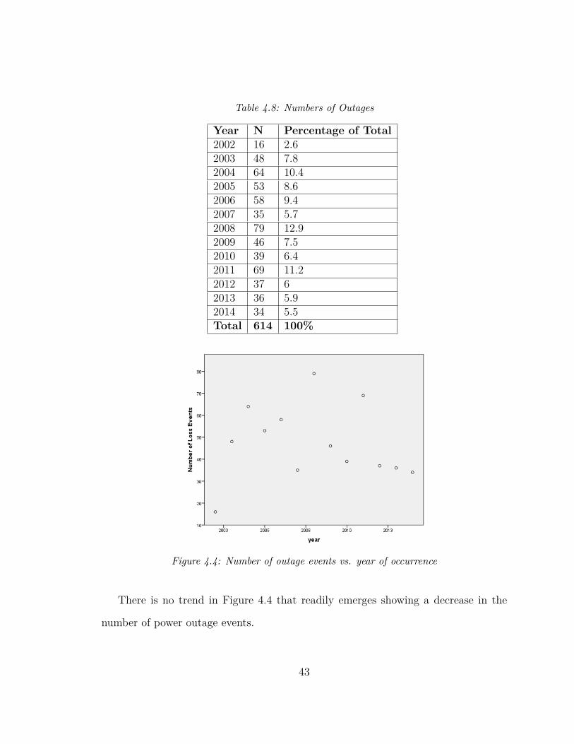
Table 4.8: Numbers of Outages
Year N Percentage of Total2002 16 2.62003 48 7.82004 64 10.42005 53 8.62006 58 9.42007 35 5.72008 79 12.92009 46 7.52010 39 6.42011 69 11.22012 37 62013 36 5.92014 34 5.5Total 614 100%
Figure 4.4: Number of outage events vs. year of occurrence
There is no trend in Figure 4.4 that readily emerges showing a decrease in the
number of power outage events.
43
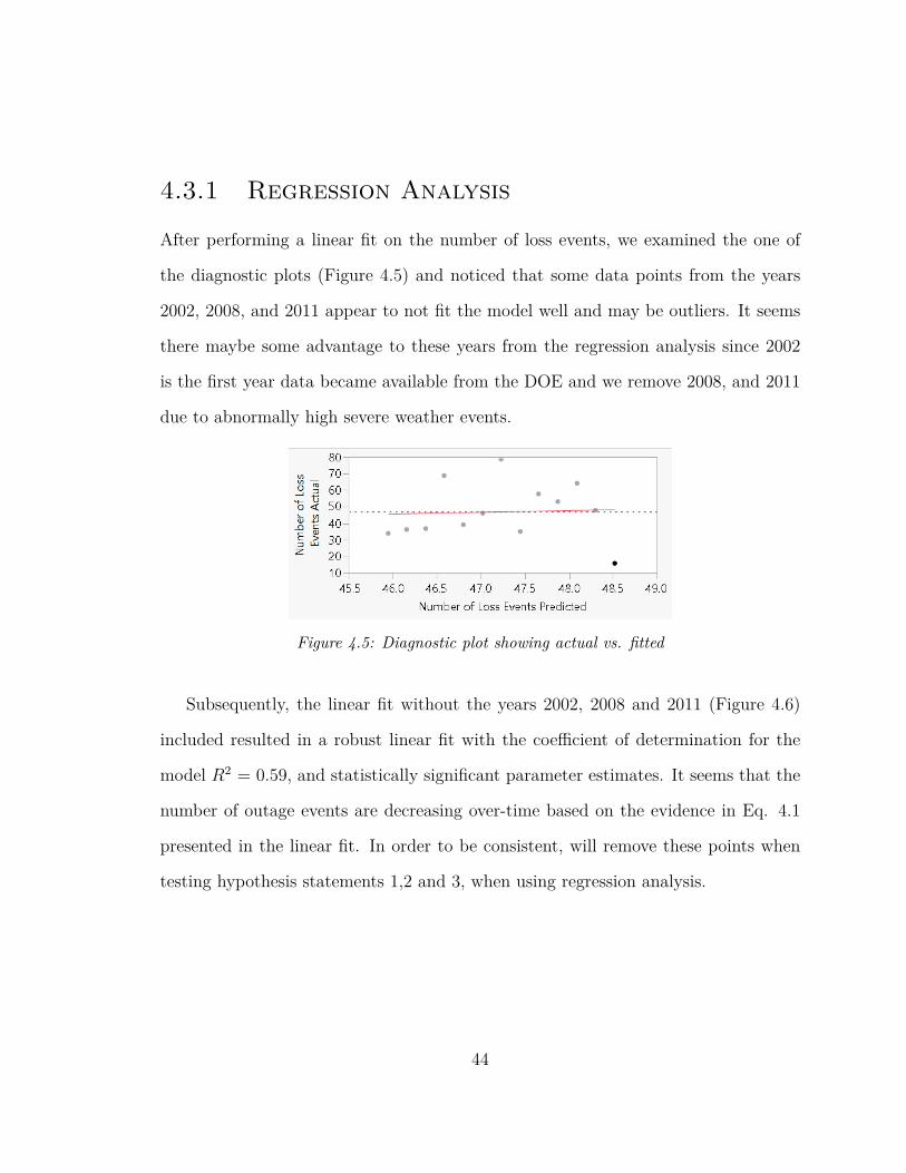
4.3.1 Regression Analysis
After performing a linear fit on the number of loss events, we examined the one of
the diagnostic plots (Figure 4.5) and noticed that some data points from the years
2002, 2008, and 2011 appear to not fit the model well and may be outliers. It seems
there maybe some advantage to these years from the regression analysis since 2002
is the first year data became available from the DOE and we remove 2008, and 2011
due to abnormally high severe weather events.
Figure 4.5: Diagnostic plot showing actual vs. fitted
Subsequently, the linear fit without the years 2002, 2008 and 2011 (Figure 4.6)
included resulted in a robust linear fit with the coefficient of determination for the
model R2 = 0.59, and statistically significant parameter estimates. It seems that the
number of outage events are decreasing over-time based on the evidence in Eq. 4.1
presented in the linear fit. In order to be consistent, will remove these points when
testing hypothesis statements 1,2 and 3, when using regression analysis.
44
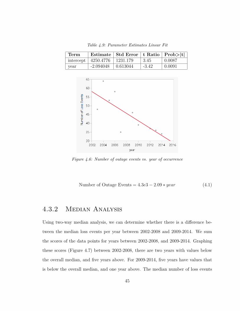
Table 4.9: Parameter Estimates Linear Fit
Term Estimate Std Error t Ratio Prob>|t|intercept 4250.4776 1231.179 3.45 0.0087year -2.094048 0.613044 -3.42 0.0091
Figure 4.6: Number of outage events vs. year of occurrence
Number of Outage Events = 4.3e3− 2.09 ∗ year (4.1)
4.3.2 Median Analysis
Using two-way median analysis, we can determine whether there is a difference be-
tween the median loss events per year between 2002-2008 and 2009-2014. We sum
the scores of the data points for years between 2002-2008, and 2009-2014. Graphing
these scores (Figure 4.7) between 2002-2008, there are two years with values below
the overall median, and five years above. For 2009-2014, five years have values that
is below the overall median, and one year above. The median number of loss events
45
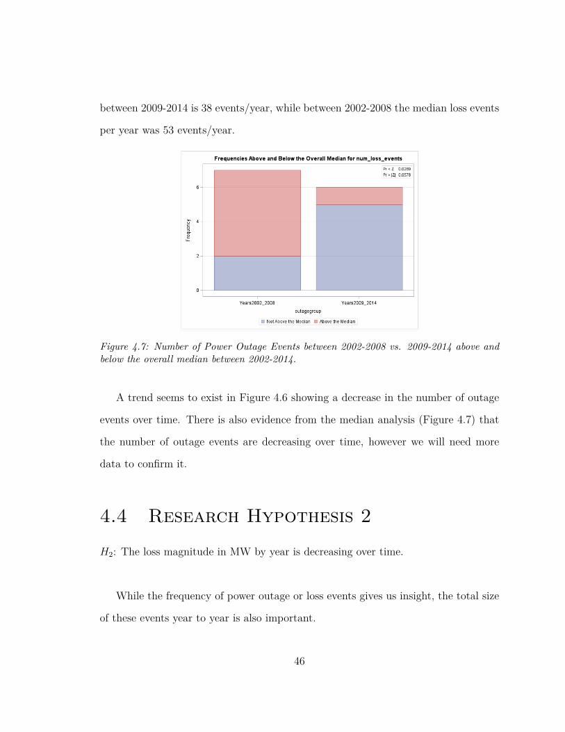
between 2009-2014 is 38 events/year, while between 2002-2008 the median loss events
per year was 53 events/year.
Figure 4.7: Number of Power Outage Events between 2002-2008 vs. 2009-2014 above andbelow the overall median between 2002-2014.
A trend seems to exist in Figure 4.6 showing a decrease in the number of outage
events over time. There is also evidence from the median analysis (Figure 4.7) that
the number of outage events are decreasing over time, however we will need more
data to confirm it.
4.4 Research Hypothesis 2
H2: The loss magnitude in MW by year is decreasing over time.
While the frequency of power outage or loss events gives us insight, the total size
of these events year to year is also important.
46
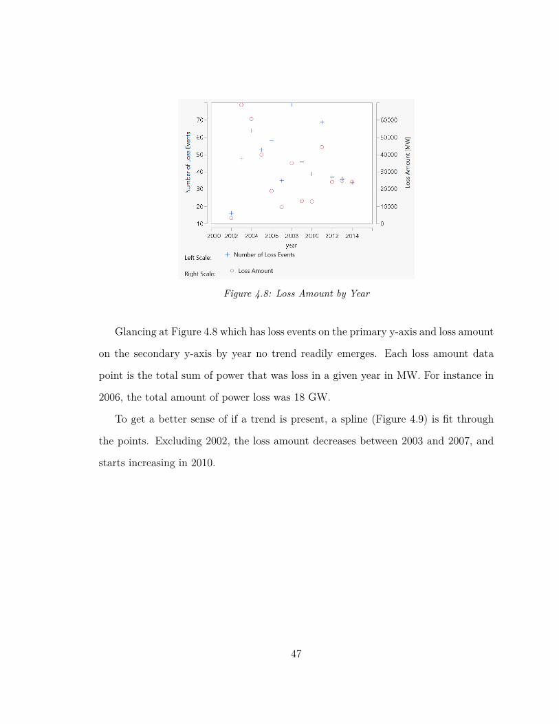
Figure 4.8: Loss Amount by Year
Glancing at Figure 4.8 which has loss events on the primary y-axis and loss amount
on the secondary y-axis by year no trend readily emerges. Each loss amount data
point is the total sum of power that was loss in a given year in MW. For instance in
2006, the total amount of power loss was 18 GW.
To get a better sense of if a trend is present, a spline (Figure 4.9) is fit through
the points. Excluding 2002, the loss amount decreases between 2003 and 2007, and
starts increasing in 2010.
47
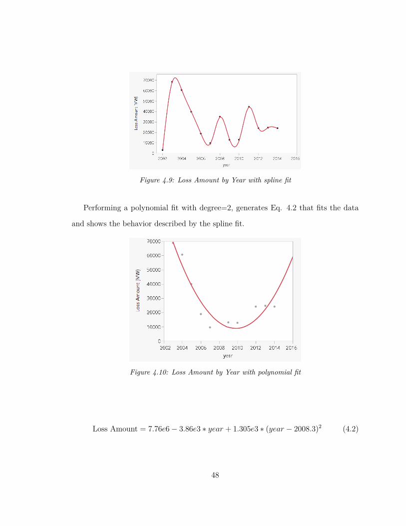
Figure 4.9: Loss Amount by Year with spline fit
Performing a polynomial fit with degree=2, generates Eq. 4.2 that fits the data
and shows the behavior described by the spline fit.
Figure 4.10: Loss Amount by Year with polynomial fit
Loss Amount = 7.76e6− 3.86e3 ∗ year + 1.305e3 ∗ (year − 2008.3)2 (4.2)
48
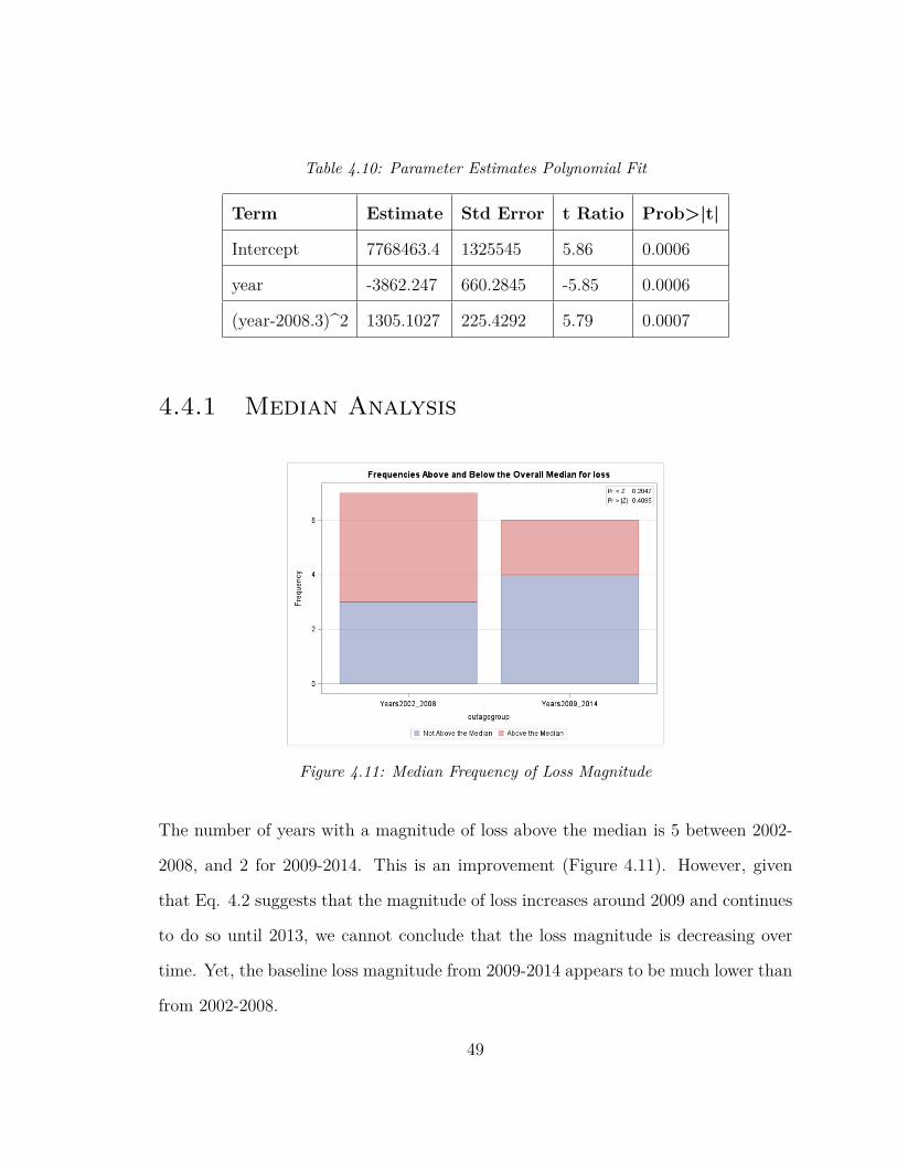
Table 4.10: Parameter Estimates Polynomial Fit
Term Estimate Std Error t Ratio Prob>|t|
Intercept 7768463.4 1325545 5.86 0.0006
year -3862.247 660.2845 -5.85 0.0006
(year-2008.3)^2 1305.1027 225.4292 5.79 0.0007
4.4.1 Median Analysis
Figure 4.11: Median Frequency of Loss Magnitude
The number of years with a magnitude of loss above the median is 5 between 2002-
2008, and 2 for 2009-2014. This is an improvement (Figure 4.11). However, given
that Eq. 4.2 suggests that the magnitude of loss increases around 2009 and continues
to do so until 2013, we cannot conclude that the loss magnitude is decreasing over
time. Yet, the baseline loss magnitude from 2009-2014 appears to be much lower than
from 2002-2008.
49
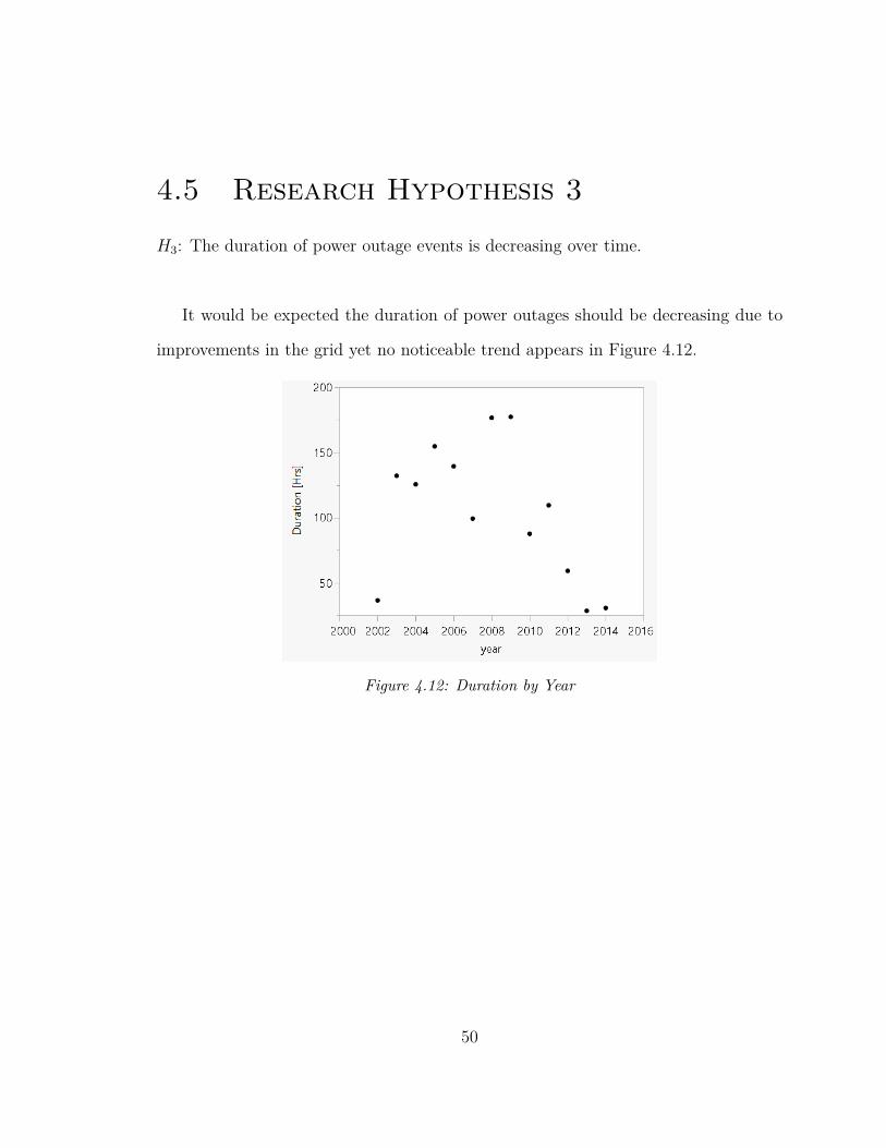
4.5 Research Hypothesis 3
H3: The duration of power outage events is decreasing over time.
It would be expected the duration of power outages should be decreasing due to
improvements in the grid yet no noticeable trend appears in Figure 4.12.
Figure 4.12: Duration by Year
50
4.5.1 Regression Analysis
Figure 4.13: Duration by Year Linear Regression
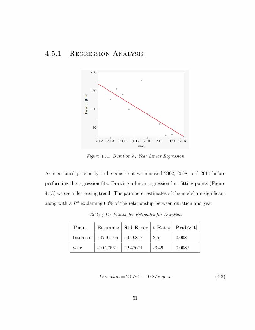
As mentioned previously to be consistent we removed 2002, 2008, and 2011 before
performing the regression fits. Drawing a linear regression line fitting points (Figure
4.13) we see a decreasing trend. The parameter estimates of the model are significant
along with a R2 explaining 60% of the relationship between duration and year.
Table 4.11: Parameter Estimates for Duration
Term Estimate Std Error t Ratio Prob>|t|
Intercept 20740.105 5919.817 3.5 0.008
year -10.27561 2.947671 -3.49 0.0082
Duration = 2.07e4− 10.27 ∗ year (4.3)
51
4.5.2 Median Analysis
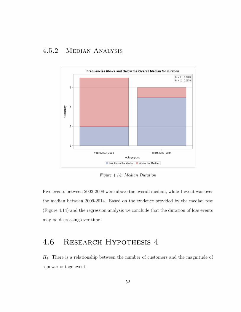
Figure 4.14: Median Duration
Five events between 2002-2008 were above the overall median, while 1 event was over
the median between 2009-2014. Based on the evidence provided by the median test
(Figure 4.14) and the regression analysis we conclude that the duration of loss events
may be decreasing over time.
4.6 Research Hypothesis 4
H4: There is a relationship between the number of customers and the magnitude of
a power outage event.
52
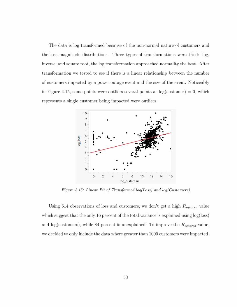
The data is log transformed because of the non-normal nature of customers and
the loss magnitude distributions. Three types of transformations were tried: log,
inverse, and square root, the log transformation approached normality the best. After
transformation we tested to see if there is a linear relationship between the number
of customers impacted by a power outage event and the size of the event. Noticeably
in Figure 4.15, some points were outliers several points at log(customer) = 0, which
represents a single customer being impacted were outliers.
Figure 4.15: Linear Fit of Transformed log(Loss) and log(Customers)
Using 614 observations of loss and customers, we don’t get a high Rsquared value
which suggest that the only 16 percent of the total variance is explained using log(loss)
and log(customers), while 84 percent is unexplained. To improve the Rsquared value,
we decided to only include the data where greater than 1000 customers were impacted.
53
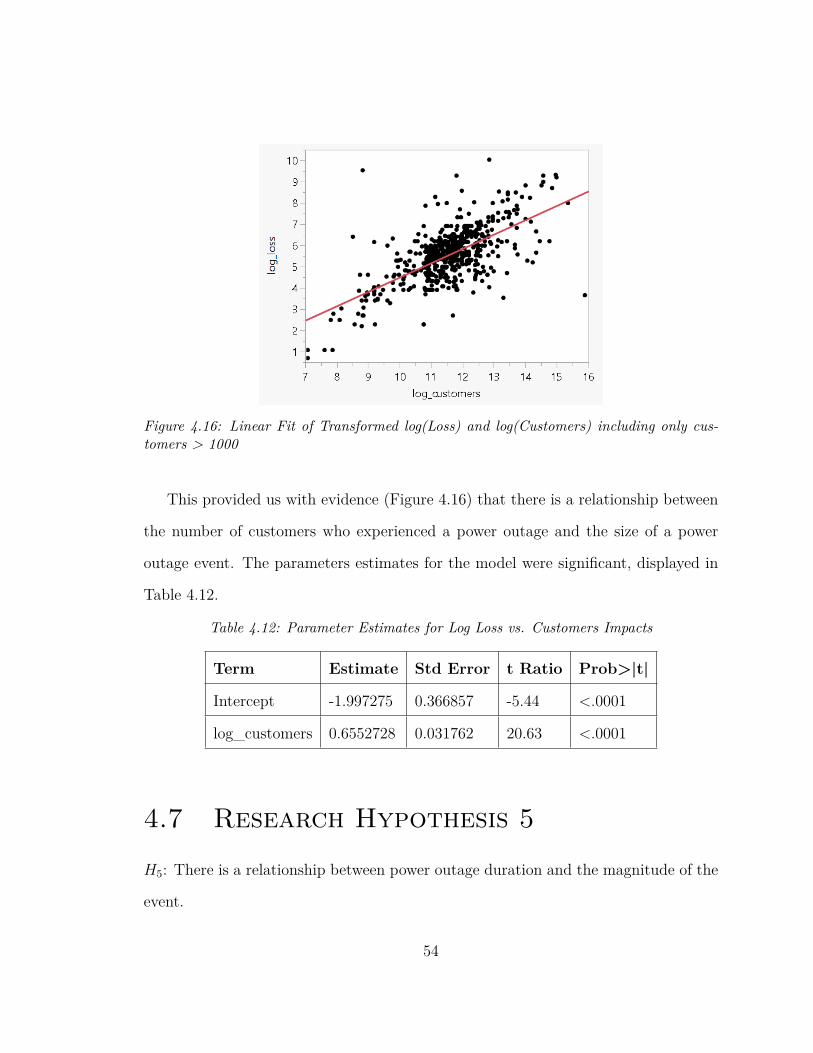
Figure 4.16: Linear Fit of Transformed log(Loss) and log(Customers) including only cus-tomers > 1000
This provided us with evidence (Figure 4.16) that there is a relationship between
the number of customers who experienced a power outage and the size of a power
outage event. The parameters estimates for the model were significant, displayed in
Table 4.12.
Table 4.12: Parameter Estimates for Log Loss vs. Customers Impacts
Term Estimate Std Error t Ratio Prob>|t|
Intercept -1.997275 0.366857 -5.44 <.0001
log_customers 0.6552728 0.031762 20.63 <.0001
4.7 Research Hypothesis 5
H5: There is a relationship between power outage duration and the magnitude of the
event.
54
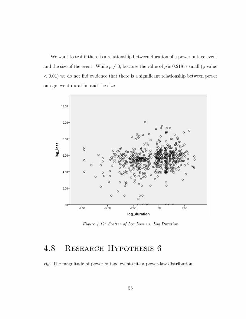
We want to test if there is a relationship between duration of a power outage event
and the size of the event. While ρ 6= 0, because the value of ρ is 0.218 is small (p-value
< 0.01) we do not fnd evidence that there is a significant relationship between power
outage event duration and the size.
Figure 4.17: Scatter of Log Loss vs. Log Duration
4.8 Research Hypothesis 6
H6: The magnitude of power outage events fits a power-law distribution.
55
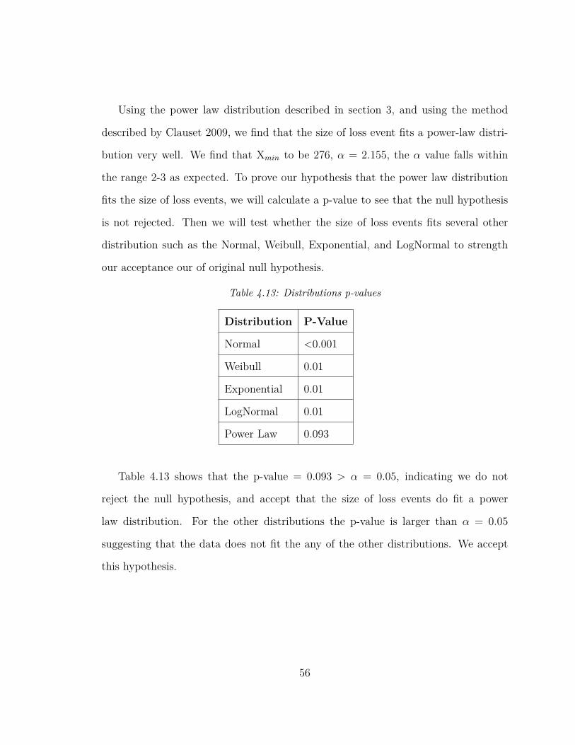
Using the power law distribution described in section 3, and using the method
described by Clauset 2009, we find that the size of loss event fits a power-law distri-
bution very well. We find that Xmin to be 276, α = 2.155, the α value falls within
the range 2-3 as expected. To prove our hypothesis that the power law distribution
fits the size of loss events, we will calculate a p-value to see that the null hypothesis
is not rejected. Then we will test whether the size of loss events fits several other
distribution such as the Normal, Weibull, Exponential, and LogNormal to strength
our acceptance our of original null hypothesis.
Table 4.13: Distributions p-values
Distribution P-Value
Normal <0.001
Weibull 0.01
Exponential 0.01
LogNormal 0.01
Power Law 0.093
Table 4.13 shows that the p-value = 0.093 > α = 0.05, indicating we do not
reject the null hypothesis, and accept that the size of loss events do fit a power
law distribution. For the other distributions the p-value is larger than α = 0.05
suggesting that the data does not fit the any of the other distributions. We accept
this hypothesis.
56
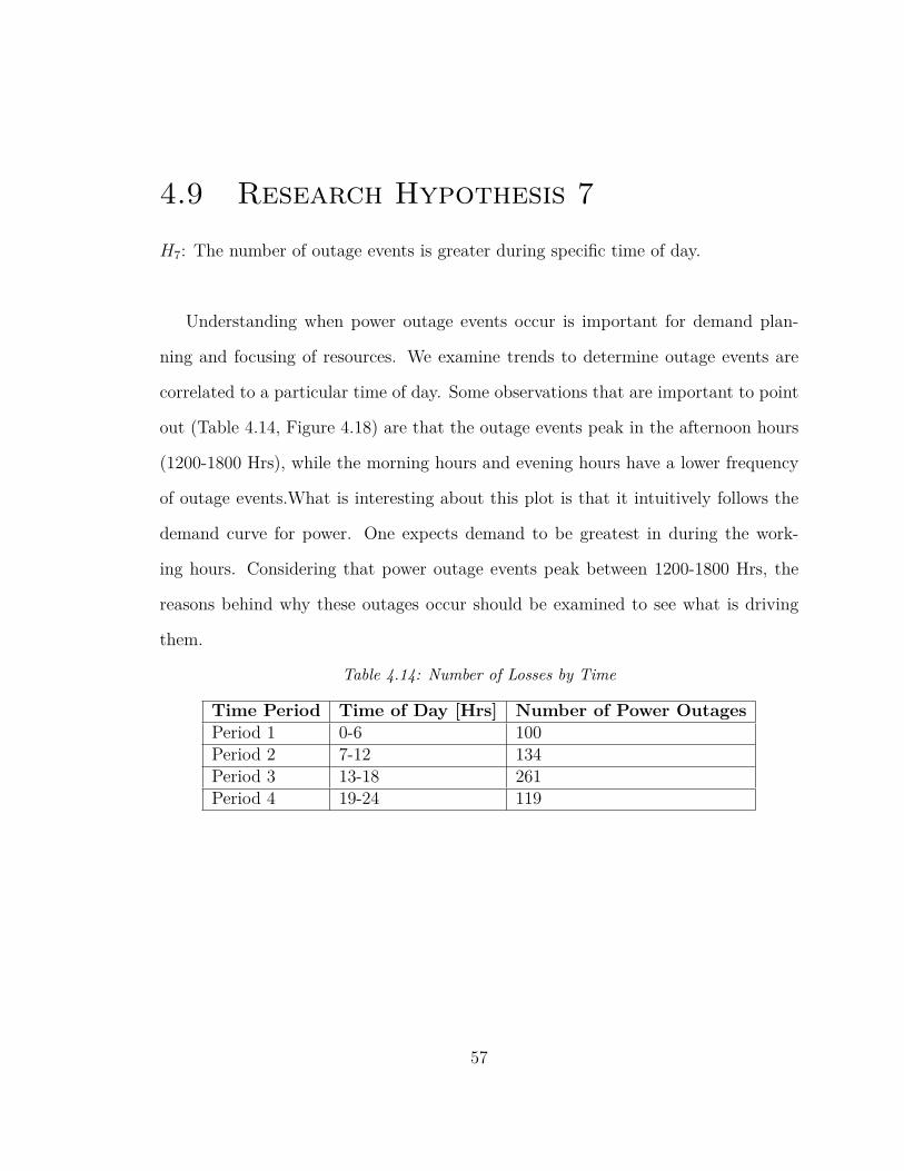
4.9 Research Hypothesis 7
H7: The number of outage events is greater during specific time of day.
Understanding when power outage events occur is important for demand plan-
ning and focusing of resources. We examine trends to determine outage events are
correlated to a particular time of day. Some observations that are important to point
out (Table 4.14, Figure 4.18) are that the outage events peak in the afternoon hours
(1200-1800 Hrs), while the morning hours and evening hours have a lower frequency
of outage events.What is interesting about this plot is that it intuitively follows the
demand curve for power. One expects demand to be greatest in during the work-
ing hours. Considering that power outage events peak between 1200-1800 Hrs, the
reasons behind why these outages occur should be examined to see what is driving
them.
Table 4.14: Number of Losses by Time
Time Period Time of Day [Hrs] Number of Power OutagesPeriod 1 0-6 100Period 2 7-12 134Period 3 13-18 261Period 4 19-24 119
57
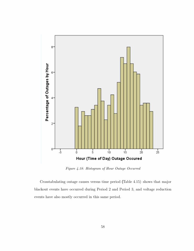
Figure 4.18: Histogram of Hour Outage Occurred
58
Crosstabulating outage causes versus time period (Table 4.15) shows that major
blackout events have occurred during Period 2 and Period 3, and voltage reduction
events have also mostly occurred in this same period.
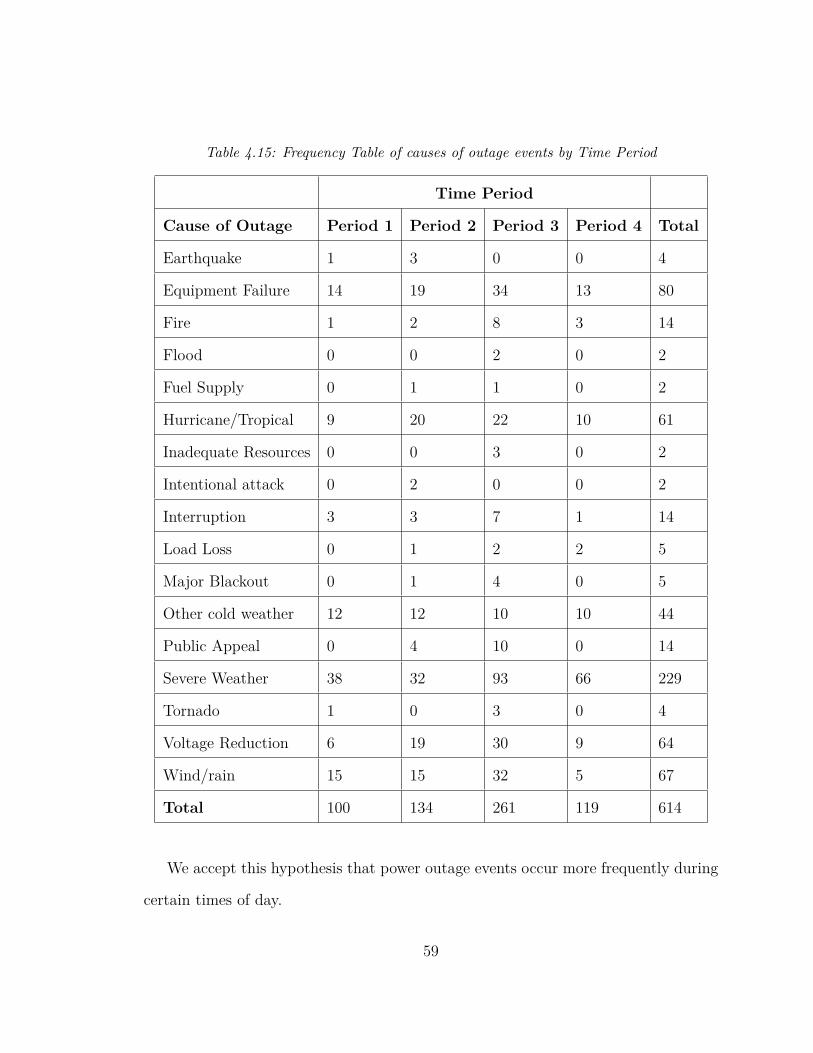
Table 4.15: Frequency Table of causes of outage events by Time Period
Time Period
Cause of Outage Period 1 Period 2 Period 3 Period 4 Total
Earthquake 1 3 0 0 4
Equipment Failure 14 19 34 13 80
Fire 1 2 8 3 14
Flood 0 0 2 0 2
Fuel Supply 0 1 1 0 2
Hurricane/Tropical 9 20 22 10 61
Inadequate Resources 0 0 3 0 2
Intentional attack 0 2 0 0 2
Interruption 3 3 7 1 14
Load Loss 0 1 2 2 5
Major Blackout 0 1 4 0 5
Other cold weather 12 12 10 10 44
Public Appeal 0 4 10 0 14
Severe Weather 38 32 93 66 229
Tornado 1 0 3 0 4
Voltage Reduction 6 19 30 9 64
Wind/rain 15 15 32 5 67
Total 100 134 261 119 614
We accept this hypothesis that power outage events occur more frequently during
certain times of day.
59
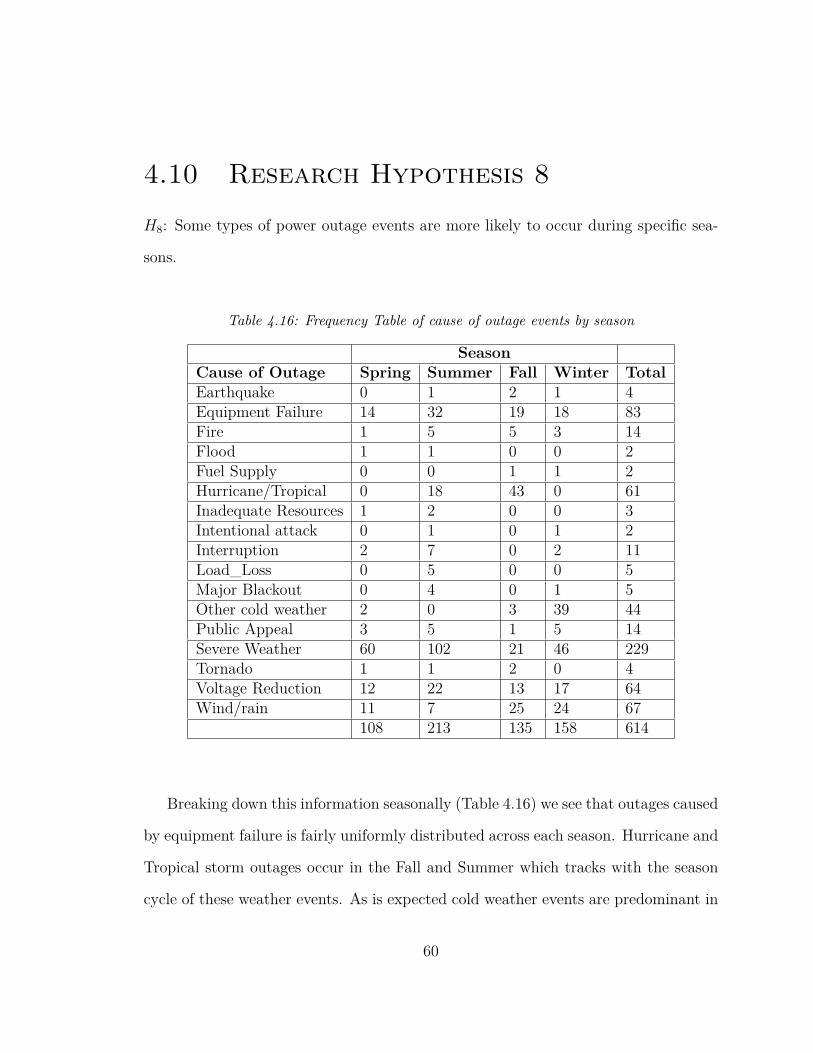
4.10 Research Hypothesis 8
H8: Some types of power outage events are more likely to occur during specific sea-
sons.
Table 4.16: Frequency Table of cause of outage events by season
SeasonCause of Outage Spring Summer Fall Winter TotalEarthquake 0 1 2 1 4Equipment Failure 14 32 19 18 83Fire 1 5 5 3 14Flood 1 1 0 0 2Fuel Supply 0 0 1 1 2Hurricane/Tropical 0 18 43 0 61Inadequate Resources 1 2 0 0 3Intentional attack 0 1 0 1 2Interruption 2 7 0 2 11Load_Loss 0 5 0 0 5Major Blackout 0 4 0 1 5Other cold weather 2 0 3 39 44Public Appeal 3 5 1 5 14Severe Weather 60 102 21 46 229Tornado 1 1 2 0 4Voltage Reduction 12 22 13 17 64Wind/rain 11 7 25 24 67
108 213 135 158 614
Breaking down this information seasonally (Table 4.16) we see that outages caused
by equipment failure is fairly uniformly distributed across each season. Hurricane and
Tropical storm outages occur in the Fall and Summer which tracks with the season
cycle of these weather events. As is expected cold weather events are predominant in
60
the Winter, while several general weather events occur during all times of year. We
accept this hypothesis that power outage events occur more frequently during certain
times of year.
4.11 Research Hypothesis 9
H9: Blackout events larger than 5000 MW are rare.
Blackout events of any size are detrimental and a nuisance, but large scale events
are more disruptive. The majority of blackout are composed of events under 300
MW and below 1000 MW (Figure 4.19), suggesting that large-scale blackouts are not
prevalent. In the restricted dataset used there were several years where there were no
blackout events greater than 5000 MW. It is important to reiterate that events under
300 MW are not required to be reported, however it appears that utilities are still
choosing to report these events. The percentage of events with loss size of at least
1000 MW, 5000 MW (Table 4.17) is 10.58%, and 2.28% respectively.
61
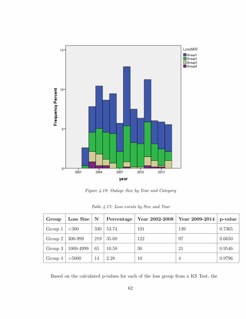
Figure 4.19: Outage Size by Year and Category
Table 4.17: Loss events by Size and Year
Group Loss Size N Percentage Year 2002-2008 Year 2009-2014 p-value
Group 1 <300 330 53.74 191 139 0.7365
Group 2 300-999 219 35.68 122 97 0.6650
Group 3 1000-4999 65 10.58 30 21 0.9546
Group 4 >5000 14 2.28 10 4 0.9796
Based on the calculated p-values for each of the loss group from a KS Test, the
62
loss size between years 2002-2008 and 2009-2014 for each loss size group (Table 4.17)
do not vary. We accept the hypothesis that Blackout events larger than 5000 MW
are rare.
4.12 Discussion
With the limited data available it seems that the number of power outage events may
be decreasing. The median number of events between 2009-2014 is lower than 2002-
2008. The linear regression trends shows that the number of loss events are decreasing
over time and the parameter estimates of the model were significant. We believe we
are justified in removing 2002, 2008, and 2011 from our regression analysis as 2002 was
the first year data was being logged by the DOE for outage events and was abnormally
low when compared to the other years. Our justification for removing 2008 and 2011
stems from the fact that these years had abnormally high severe weather events.
While the loss magnitude decreased over several years, it increased in later years.
Perhaps there has been significant progress made in infrastructure investments and
smart grid technology to prevent large loss events from occurring. It is our believe
that that the inclusion of smart grid technology is isolating outage events better and
preventing large-scale cascading outages.
There is evidence that the duration of an outage event is decreasing over time.
There could be a number of potential explanations, including additional resources
being deployed to reduce the outage duration, systems are able to restart power flow
using redundancy built in, and that outage events are being reported faster using
smart metering technology so they can be fixed quicker.
63
When we look for relationships between the number of customers and the size of a
power outage events, there is a moderate correlation. Intuitively, it makes sense that
larger loss amounts would be driven by a larger number of customers. The outliers
in the data when, log(loss) and log(customer) are plotted on an XY chart are likely
from commercial customers that have substantially large loss, but are listed as only
one customer being impacted. Surprisingly, I did not find a relationship between
power outage duration and the size of the event. I thought the larger the loss event,
the longer the duration of the event, but there is no correlation. It was interesting
that there appeared to be no correlation between the loss magnitude and duration.
Perhaps this is due to the fact that an increased amount of resources are deployed to
reduce the restoration time. Or it could be due to systems that are allowing utilities
to bring power back on-line faster.
The size of power loss events fits a power-law distribution, and does not fit any
of several other distributions tested. This exercise served as a verification of previous
research work using a new set of data.
It appears that some types of outage events are more likely to occur during certain
times of day. There is a time of day dependence for power outage with the number of
events peaking during the 1200-1800 Hrs period. This time range is the one with the
highest anticipated usage by customers, so it is expected that the largest number of
outages would come in this period. Interestingly, the number of outage events, is fairly
uniformly distributed in the other time periods. Weather accounts for around 65%
of the reasons leading to a power outage, followed by equipment failure and voltage
reduction events. Outage events during the summer are driven by Hurricane/Tropical
storm events. It has been postulated that climate change is causing more severe
64

weather which is in turn impacting our power system greatly. However, if we examine
the Table 4.15 which shows outage events by Time Period, we see that there is a usage
factor correlated to weather events. This suggests that the weather event alone is most
likely not sufficient in itself to lead to the outage and customer usage plays a large
role as usage peaks in Time Period 3 (13-18 Hrs).
Large blackout events are rare with events around 5000 MW account for 2.28%
of power outage events. Perhaps, this could be due to isolating systems from causing
cascading failures.
65
Chapter 5
Exploring Power Reliability Met-
rics and AMI deployment
5.1 Introduction
In the United States power reliability is tracked utility to utility by indices, in par-
ticular SAIFI and CAIDI. We are interested in looking at several states and utilities
to assess whether the frequency and duration of power outage events vary state to
state using SAIFI and CAIDI indices. It is our intention to test these hypotheses
mentioned in the introduction using the reliability metrics. With the inclusion of
smart grid technology we are interested in knowing whether the frequency of outage
events is decreasing with more smart meters. Previous studies have stated that 35
states including the District of Columbia mandate the reporting of reliability event
information. However, not all states make the data publicly available or make them
easy to be found on the section of the state government website dedicated to electrical
regulatory oversight. Therefore we use a convenience sample of the information that
66
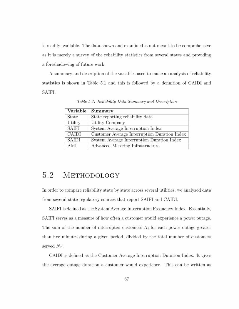
is readily available. The data shown and examined is not meant to be comprehensive
as it is merely a survey of the reliability statistics from several states and providing
a foreshadowing of future work.
A summary and description of the variables used to make an analysis of reliability
statistics is shown in Table 5.1 and this is followed by a definition of CAIDI and
SAIFI.
Table 5.1: Reliability Data Summary and Description
Variable SummaryState State reporting reliability dataUtility Utility CompanySAIFI System Average Interruption IndexCAIDI Customer Average Interruption Duration IndexSAIDI System Average Interruption Duration IndexAMI Advanced Metering Infrastructure
5.2 Methodology
In order to compare reliability state by state across several utilities, we analyzed data
from several state regulatory sources that report SAIFI and CAIDI.
SAIFI is defined as the System Average Interruption Frequency Index. Essentially,
SAIFI serves as a measure of how often a customer would experience a power outage.
The sum of the number of interrupted customers Ni for each power outage greater
than five minutes during a given period, divided by the total number of customers
served NT .
CAIDI is defined as the Customer Average Interruption Duration Index. It gives
the average outage duration a customer would experience. This can be written as
67
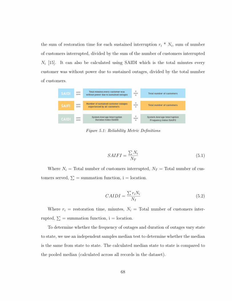
the sum of restoration time for each sustained interruption ri * Ni, sum of number
of customers interrupted, divided by the sum of the number of customers interrupted
Ni [15]. It can also be calculated using SAIDI which is the total minutes every
customer was without power due to sustained outages, divided by the total number
of customers.
Figure 5.1: Reliability Metric Definitions
SAIFI =∑Ni
NT
(5.1)
Where Ni = Total number of customers interrupted, NT = Total number of cus-
tomers served, ∑ = summation function, i = location.
CAIDI =∑riNi
NI
(5.2)
Where ri = restoration time, minutes, Ni = Total number of customers inter-
rupted, ∑ = summation function, i = location.
To determine whether the frequency of outages and duration of outages vary state
to state, we use an independent samples median test to determine whether the median
is the same from state to state. The calculated median state to state is compared to
the pooled median (calculated across all records in the dataset).
68
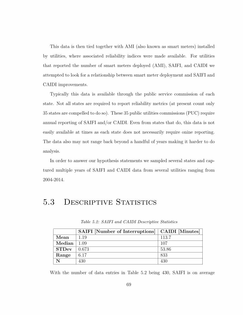
This data is then tied together with AMI (also known as smart meters) installed
by utilities, where associated reliability indices were made available. For utilities
that reported the number of smart meters deployed (AMI), SAIFI, and CAIDI we
attempted to look for a relationship between smart meter deployment and SAIFI and
CAIDI improvements.
Typically this data is available through the public service commission of each
state. Not all states are required to report reliability metrics (at present count only
35 states are compelled to do so). These 35 public utilities commissions (PUC) require
annual reporting of SAIFI and/or CAIDI. Even from states that do, this data is not
easily available at times as each state does not necessarily require onine reporting.
The data also may not range back beyond a handful of years making it harder to do
analysis.
In order to answer our hypothesis statements we sampled several states and cap-
tured multiple years of SAIFI and CAIDI data from several utilities ranging from
2004-2014.
5.3 Descriptive Statistics
Table 5.2: SAIFI and CAIDI Descriptive Statistics
SAIFI [Number of Interruptions] CAIDI [Minutes]Mean 1.19 113.7Median 1.09 107STDev 0.673 53.86Range 6.17 833N 430 430
With the number of data entries in Table 5.2 being 430, SAIFI is on average
69
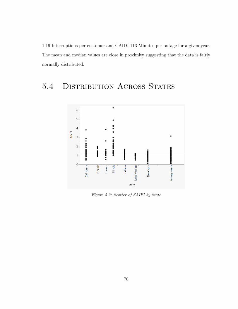
1.19 Interruptions per customer and CAIDI 113 Minutes per outage for a given year.
The mean and median values are close in proximity suggesting that the data is fairly
normally distributed.
5.4 Distribution Across States
Figure 5.2: Scatter of SAIFI by State
70
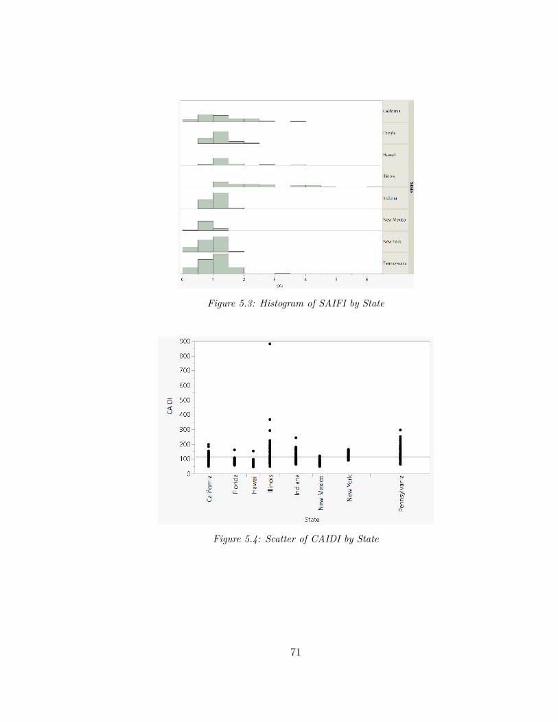
Figure 5.3: Histogram of SAIFI by State
Figure 5.4: Scatter of CAIDI by State
71
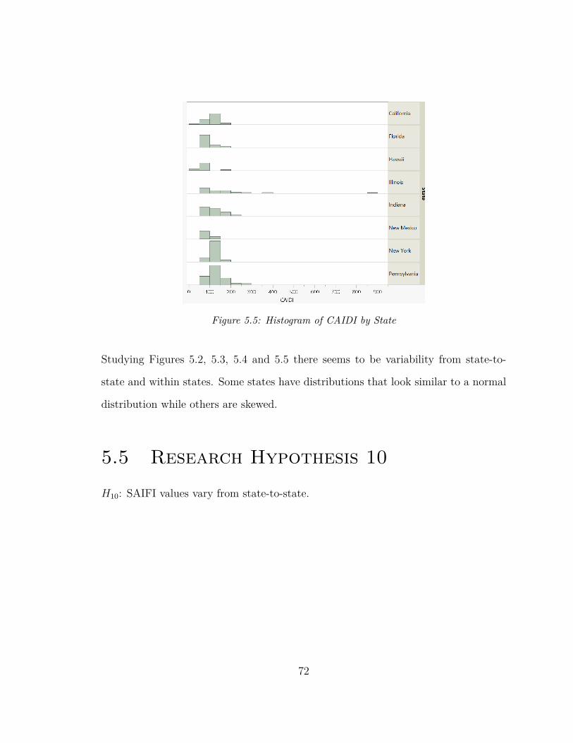
Figure 5.5: Histogram of CAIDI by State
Studying Figures 5.2, 5.3, 5.4 and 5.5 there seems to be variability from state-to-
state and within states. Some states have distributions that look similar to a normal
distribution while others are skewed.
5.5 Research Hypothesis 10
H10: SAIFI values vary from state-to-state.
72
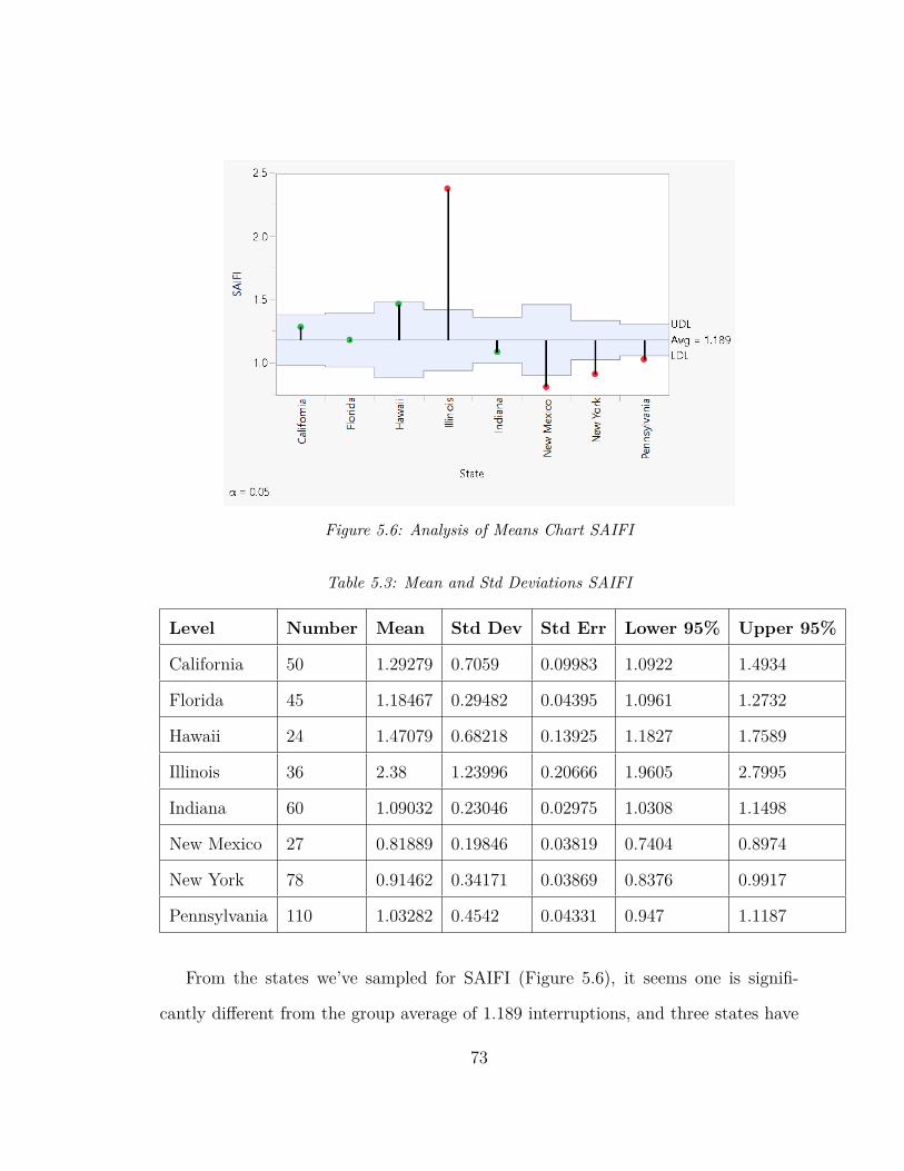
Figure 5.6: Analysis of Means Chart SAIFI
Table 5.3: Mean and Std Deviations SAIFI
Level Number Mean Std Dev Std Err Lower 95% Upper 95%
California 50 1.29279 0.7059 0.09983 1.0922 1.4934
Florida 45 1.18467 0.29482 0.04395 1.0961 1.2732
Hawaii 24 1.47079 0.68218 0.13925 1.1827 1.7589
Illinois 36 2.38 1.23996 0.20666 1.9605 2.7995
Indiana 60 1.09032 0.23046 0.02975 1.0308 1.1498
New Mexico 27 0.81889 0.19846 0.03819 0.7404 0.8974
New York 78 0.91462 0.34171 0.03869 0.8376 0.9917
Pennsylvania 110 1.03282 0.4542 0.04331 0.947 1.1187
From the states we’ve sampled for SAIFI (Figure 5.6), it seems one is signifi-
cantly different from the group average of 1.189 interruptions, and three states have
73
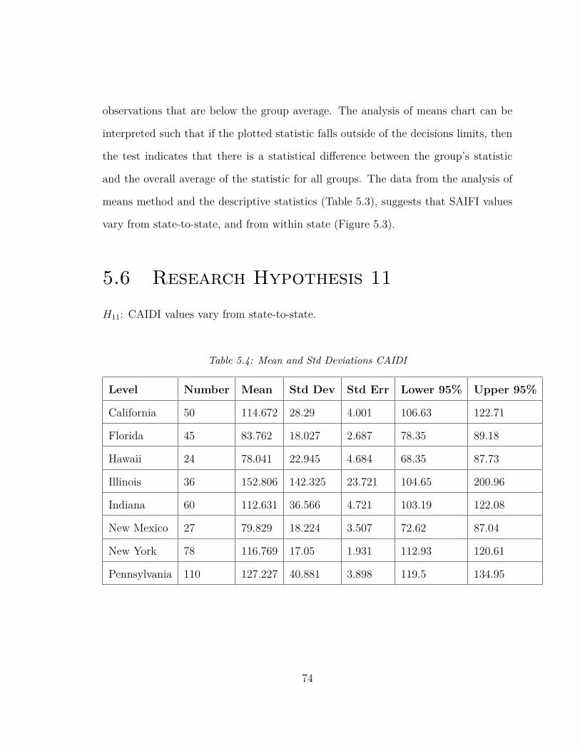
observations that are below the group average. The analysis of means chart can be
interpreted such that if the plotted statistic falls outside of the decisions limits, then
the test indicates that there is a statistical difference between the group’s statistic
and the overall average of the statistic for all groups. The data from the analysis of
means method and the descriptive statistics (Table 5.3), suggests that SAIFI values
vary from state-to-state, and from within state (Figure 5.3).
5.6 Research Hypothesis 11
H11: CAIDI values vary from state-to-state.
Table 5.4: Mean and Std Deviations CAIDI
Level Number Mean Std Dev Std Err Lower 95% Upper 95%
California 50 114.672 28.29 4.001 106.63 122.71
Florida 45 83.762 18.027 2.687 78.35 89.18
Hawaii 24 78.041 22.945 4.684 68.35 87.73
Illinois 36 152.806 142.325 23.721 104.65 200.96
Indiana 60 112.631 36.566 4.721 103.19 122.08
New Mexico 27 79.829 18.224 3.507 72.62 87.04
New York 78 116.769 17.05 1.931 112.93 120.61
Pennsylvania 110 127.227 40.881 3.898 119.5 134.95
74
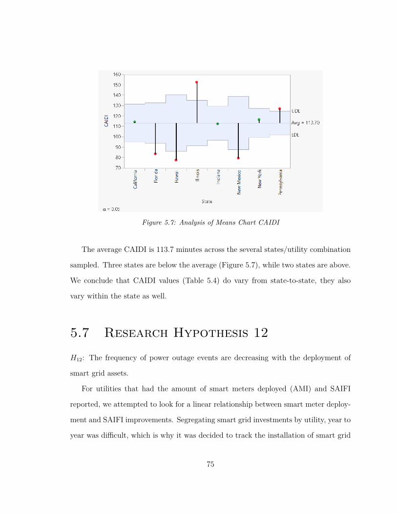
Figure 5.7: Analysis of Means Chart CAIDI
The average CAIDI is 113.7 minutes across the several states/utility combination
sampled. Three states are below the average (Figure 5.7), while two states are above.
We conclude that CAIDI values (Table 5.4) do vary from state-to-state, they also
vary within the state as well.
5.7 Research Hypothesis 12
H12: The frequency of power outage events are decreasing with the deployment of
smart grid assets.
For utilities that had the amount of smart meters deployed (AMI) and SAIFI
reported, we attempted to look for a linear relationship between smart meter deploy-
ment and SAIFI improvements. Segregating smart grid investments by utility, year to
year was difficult, which is why it was decided to track the installation of smart grid
75
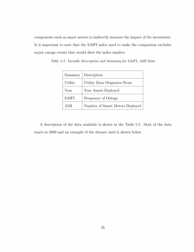
components such as smart meters to indirectly measure the impact of the investment.
It is important to note that the SAIFI index used to make the comparison excludes
major outage events that would skew the index number.
Table 5.5: Variable Description and Summary for SAIFI, AMI Data
Summary Description
Utility Utility Data Originates From
Year Year Assets Deployed
SAIFI Frequency of Outage
AMI Number of Smart Meters Deployed
A description of the data available is shown in the Table 5.5. Most of the data
starts in 2009 and an example of the dataset used is shown below.
76
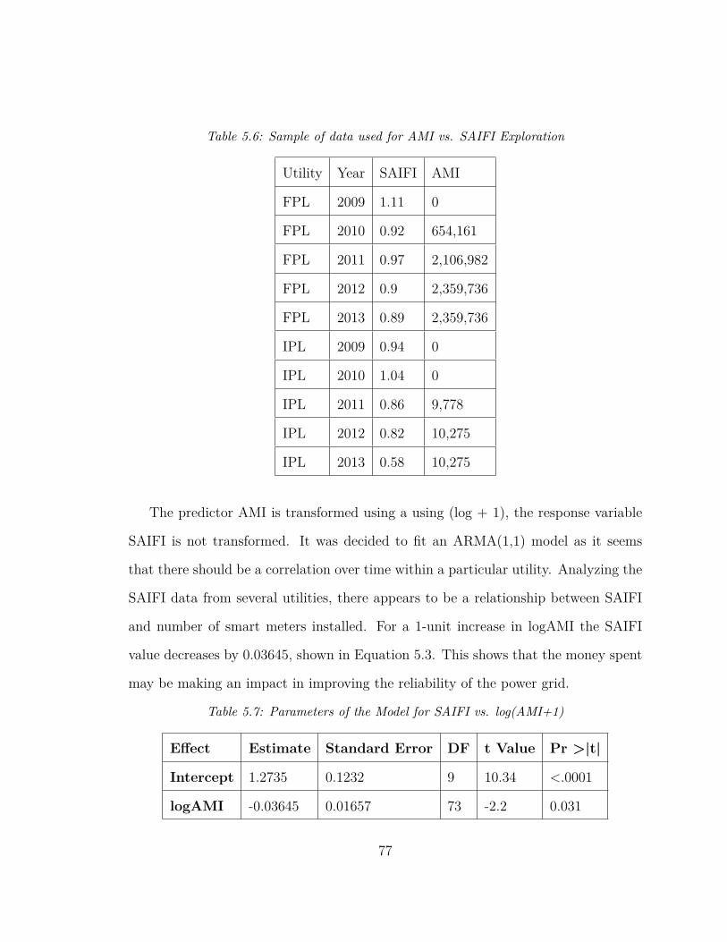
Table 5.6: Sample of data used for AMI vs. SAIFI Exploration
Utility Year SAIFI AMI
FPL 2009 1.11 0
FPL 2010 0.92 654,161
FPL 2011 0.97 2,106,982
FPL 2012 0.9 2,359,736
FPL 2013 0.89 2,359,736
IPL 2009 0.94 0
IPL 2010 1.04 0
IPL 2011 0.86 9,778
IPL 2012 0.82 10,275
IPL 2013 0.58 10,275
The predictor AMI is transformed using a using (log + 1), the response variable
SAIFI is not transformed. It was decided to fit an ARMA(1,1) model as it seems
that there should be a correlation over time within a particular utility. Analyzing the
SAIFI data from several utilities, there appears to be a relationship between SAIFI
and number of smart meters installed. For a 1-unit increase in logAMI the SAIFI
value decreases by 0.03645, shown in Equation 5.3. This shows that the money spent
may be making an impact in improving the reliability of the power grid.
Table 5.7: Parameters of the Model for SAIFI vs. log(AMI+1)
Effect Estimate Standard Error DF t Value Pr >|t|
Intercept 1.2735 0.1232 9 10.34 <.0001
logAMI -0.03645 0.01657 73 -2.2 0.031
77
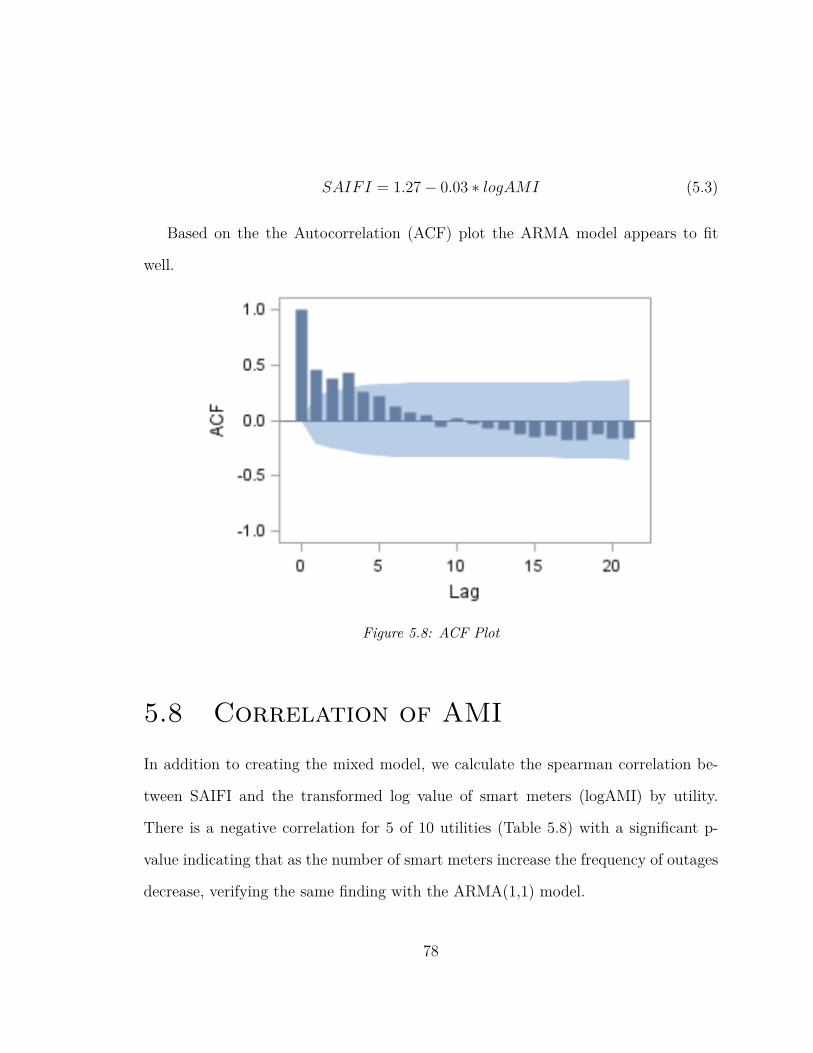
SAIFI = 1.27− 0.03 ∗ logAMI (5.3)
Based on the the Autocorrelation (ACF) plot the ARMA model appears to fit
well.
Figure 5.8: ACF Plot
5.8 Correlation of AMI
In addition to creating the mixed model, we calculate the spearman correlation be-
tween SAIFI and the transformed log value of smart meters (logAMI) by utility.
There is a negative correlation for 5 of 10 utilities (Table 5.8) with a significant p-
value indicating that as the number of smart meters increase the frequency of outages
decrease, verifying the same finding with the ARMA(1,1) model.
78
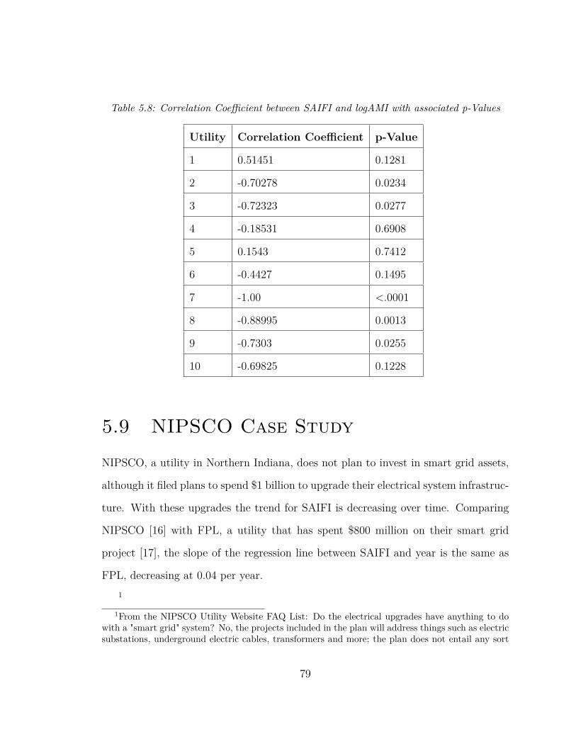
Table 5.8: Correlation Coefficient between SAIFI and logAMI with associated p-Values
Utility Correlation Coefficient p-Value
1 0.51451 0.1281
2 -0.70278 0.0234
3 -0.72323 0.0277
4 -0.18531 0.6908
5 0.1543 0.7412
6 -0.4427 0.1495
7 -1.00 <.0001
8 -0.88995 0.0013
9 -0.7303 0.0255
10 -0.69825 0.1228
5.9 NIPSCO Case Study
NIPSCO, a utility in Northern Indiana, does not plan to invest in smart grid assets,
although it filed plans to spend $1 billion to upgrade their electrical system infrastruc-
ture. With these upgrades the trend for SAIFI is decreasing over time. Comparing
NIPSCO [16] with FPL, a utility that has spent $800 million on their smart grid
project [17], the slope of the regression line between SAIFI and year is the same as
FPL, decreasing at 0.04 per year.1
1From the NIPSCO Utility Website FAQ List: Do the electrical upgrades have anything to dowith a "smart grid" system? No, the projects included in the plan will address things such as electricsubstations, underground electric cables, transformers and more; the plan does not entail any sort
79
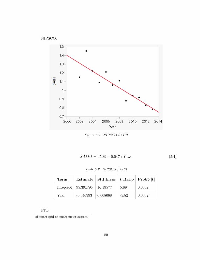
NIPSCO:
Figure 5.9: NIPSCO SAIFI
SAIFI = 95.39− 0.047 ∗ Y ear (5.4)
Table 5.9: NIPSCO SAIFI
Term Estimate Std Error t Ratio Prob>|t|
Intercept 95.391795 16.19577 5.89 0.0002
Year -0.046993 0.008068 -5.82 0.0002
FPL:of smart grid or smart meter system.
80
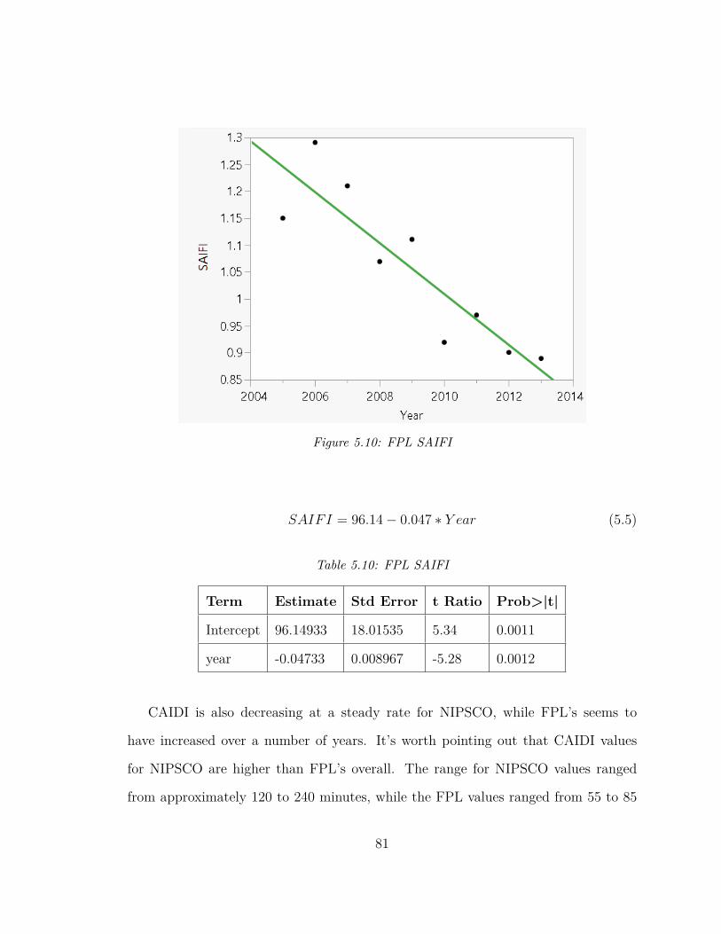
Figure 5.10: FPL SAIFI
SAIFI = 96.14− 0.047 ∗ Y ear (5.5)
Table 5.10: FPL SAIFI
Term Estimate Std Error t Ratio Prob>|t|
Intercept 96.14933 18.01535 5.34 0.0011
year -0.04733 0.008967 -5.28 0.0012
CAIDI is also decreasing at a steady rate for NIPSCO, while FPL’s seems to
have increased over a number of years. It’s worth pointing out that CAIDI values
for NIPSCO are higher than FPL’s overall. The range for NIPSCO values ranged
from approximately 120 to 240 minutes, while the FPL values ranged from 55 to 85
81
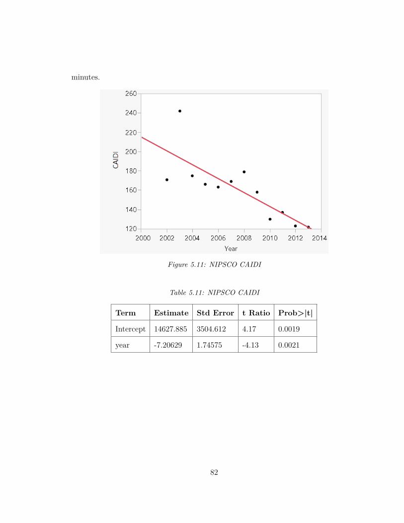
minutes.
Figure 5.11: NIPSCO CAIDI
Table 5.11: NIPSCO CAIDI
Term Estimate Std Error t Ratio Prob>|t|
Intercept 14627.885 3504.612 4.17 0.0019
year -7.20629 1.74575 -4.13 0.0021
82
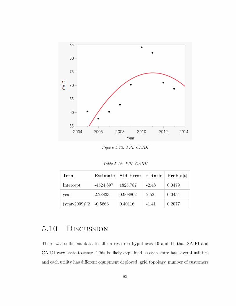
Figure 5.12: FPL CAIDI
Table 5.12: FPL CAIDI
Term Estimate Std Error t Ratio Prob>|t|
Intercept -4524.897 1825.787 -2.48 0.0479
year 2.28833 0.908802 2.52 0.0454
(year-2009)^2 -0.5663 0.40116 -1.41 0.2077
5.10 Discussion
There was sufficient data to affirm research hypothesis 10 and 11 that SAIFI and
CAIDI vary state-to-state. This is likely explained as each state has several utilities
and each utility has different equipment deployed, grid topology, number of customers
83
and age of equipment.
The ARMA model created shows there may be reduction of power outage events
as the number of smart grid assets are being deployed.The ARMA model created sug-
gests that there is a reduction in average number of power outage events per customer
[SAIFI] as the number of smart meters deployed increase. We cannot definitively tie
the reduction in the SAIFI to an increase of smart meters, due to other confounding
variables that may be present, but the evidence is encouraging and hypothesis 12 may
be confirmed in the future with more data. This was further verified with correlation
coefficients greater than 0.70 for 5 out of 10 utilities SAIFI, documented in Table 5.8.
The NIPSCO vs. FPL case study makes us think about what factors are most
important in reducing SAIFI values. It shows smart grid assets may not be the only
thing reducing SAIFI and CAIDI. Factors other than smart meters may be helping
FPL decrease their SAIFI and CAIDI values.
84
Chapter 6
Recommendations and Conclusion
The previous chapters provide a detailed analysis of power outage events and electrical
reliability metrics. Additionally we stated the conclusions that we drew from these
each of the hypothesis statements that we tested. In this chapter we will discuss
factors that interfered with our analysis, recommendations for utilities and policy
makers, and information that would be more helpful for research to draw more solid
conclusions.
After concluding our analysis in the subsquent chapters, we need to ask how this
information should used to better inform the general public, public policy makers,
and public utilities companies to make better decisions.
6.1 Confounding Variables
There were several variables that interfered with our ability to answer certain research
hypothesis or questions. Initially we wanted to correlate smart grid funding to an
improvement in reliability indices. This was difficult because the spending on all
85
smart grid assets is not broken down year by year for a given utility. This lead
us to use the deployment of specific smart grid assets which was broken down year
by year as an indirect measure of smart grid funding. These assets include smart
meter infrastructure (AMI), Autofeeders (AF) and Phase Monitoring Units (PMUs).
However, there is only sufficient data from smart meter assets to draw any inference.
Consequently, we don’t know the impact of the other two smart grid assets that
were being deployed. Furthermore, we only analyzed data from utilities that received
smart grid funding from the government because some utilities do not exactly report
how they are spending their money.
We also wanted to do a correlation between the number of outage events and
region, but this was not possible because some outage events were listed as impacting
multiple locations. This is likely evidence of a cascading failure, but we are not
sure whether or not this is true. Because the magnitude, duration, and number of
customers impacted was not always available, we eliminated these observations. We
could have estimated these values but we chose not to given that we might use a false
assumption to estimate them. Another confounding factor is that utility reliability
data is heavily based on the service area (above ground, underground lines), rural or
urban, types of assets, and age of assets. This information is not readily available, so
it hard to adjust for these factors as we perform analysis.
86
6.2 Using the Data to make better de-
cisions
Based on the data we draw several conclusions and recommendations for focus points.
Weather accounts for nearly 67% of the recorded electrical disturbances. In unison
with smart grid asset deployment, infrastructure needs to be reinforced to be resilient
against weather events. The benefits realized from this would include a reduction in
overburden on repair crews to restore power after storms. Aging infrastructure needs
to be replaced with new equipment, and risk analysis needs to be undertaken to figure
out which assets to replace first through the use of cost-benefit analysis.
From a seasonal perspective it makes sense to have more repair crews on hand
during storm events in the summer and winter based on the projected meteorology
forecasts. As a higher call volume is expected from customers reporting outage events,
more staff should be on hand to assist customers in reporting outages and proving
information when power will return. If cellular networks are not impacted, SMS alerts
(Text Messaging Alerts) could be sent or customers could report outages by SMS.
A number of companies are turning to social media channels such as Twitter and
Facebook to spread their message.
It is our opinion that short outages (5 minutes or less) occurring infrequently is
preferred over long sustained power outages. Thus there is a valid question as to
whether a trade-off could be achieved by ensuring that longer events are significantly
reduced at the expense of more shorter duration outages. Considering commercial
customers are impacted the greatest should resources be focused to make sure they
87
are better protected, or perhaps should commercial customers protect themselves by
adding backup systems? Perhaps a discount in service rates could be given for such
an agreement.
From a consumer perspective, Time-of-Use (TOU) pricing could be implemented
to encourage consumers to use power outside of the highest demand windows (1200-
1800 Hrs), by charging less for electricity during non-peak hours. This would help
the utility in preparing for demand by reducing the number of outage events. Even if
TOU is not implemented, the time of outage data gives us insight into telling power
utilities that they should add more capacity during hours likely to be impacted by
outage events.
6.3 Data Available
Utilities, Academics, the Government, are going to continue be looking at correlations
between smart grid asset deployment, funding, and reliability metrics. Requiring that
detailed and more accessible data from the DOE and Utilities be available would
allow conclusions to be drawn from it more quickly. It would be useful in having
SAIFI, CAIDI, year, smart grid assets deployed including AMI, PMU, and AF. This
information may be available from several sources. For instance, SAIFI and CAIDI
are available from state utility regulators for states requiring reporting, but smart grid
asset deployment data is not necessarily required. Furthermore, having the number of
customers, number of lines above ground and below ground, and age of infrastructure
would allow conclusions to be drawn between age of the infrastructure and reliability.
It is our opinion that more information needs to be available (such as Number of
88
Customers served by the utility should be available, Electricity Cost, Number of Lines
Overhead, Underground) across the board so more research questions can be answered
more readily. Finding this information can be heavily time consuming and may exist
readily for one utility but not for another. It would be good to provide year-by-year
funding on smart grid assets for a particular utility, by asset type. Understandably,
it is possible that some of this information could be misused by someone looking for
a vulnerability in the grid.
6.4 Syntax recommendation
In the DOE reported Electrical Disturbance data, column locations are changed for
some years. For instance, date was in the first column in the provided spreadsheet,
followed by time of the outage and the next year date was in the second column,
while the time of the outage was in the first column. This requires manipulation of
the spreadsheet to make the data importable into a software program to analyze the
data. Manipulation must be performed manually, or by a software solution which is
a waste of a researcher taking time away from the intended purpose. Classification
of the type of disturbance are not consistently logged from entry to entry.
For example the following classifications have appeared in different years: Severe
Storms with Strong Winds, Storm with High Winds, Severe Weather vs. Severe
Storms.
This in itself highlights the importance of machine learning and data classification
algorithms to correctly classify items.
Many states do not provide data in a research friendly format for instance most
89
states do not provide data in spreadsheets, csv format, or another format that makes
data readily readable into statistic analysis software. Dealing with data in this manner
requires a lot of effort in re-transcribing the data. A potential consequence of this is
that errors can be made resulting in a incorrect understanding of the data.
6.5 Future Work
We intend to publish our findings in two papers. We will continue to explore elec-
trical disturbance data and the connection between smart grid assets and reliability
statistics. Maintaining robust and reliability electrical grid is important for America’s
growth and security.
90
Bibliography
[1] S. Chatterjee, “Michael Faraday: Discovery of electromagnetic induction,” Res-
onance, vol. 7, pp. 35–45, 2002.
[2] B. Liscouski and W. Elliot, “U.S.-Canada Power System Outage Task Force,”
US-Canada Power System Outage Task Force, no. April, p. 238, 2004.
[3] G. Andersson, P. Donalek, R. Farmer, N. Hatziargyriou, I. Kamwa, P. Kundur,
N. Martins, J. Paserba, P. Pourbeik, J. Sanchez-Gasca, R. Schulz, A. Stankovic,
C. Taylor, and V. Vittal, “Causes of the 2003 major grid blackouts in North
America Europe, and recommended means to improve system dynamic perfor-
mance,” IEEE Transactions on Power Systems, vol. 20, no. 4, pp. 1922–1928,
2005.
[4] J. Romero, “Blackouts illuminate India’s power problems,” IEEE Spectrum,
vol. 49, pp. 11–12, Oct. 2012.
[5] DOE Electriciy Delivery and Energy Reliability, “Smart Grid Investment Grant
Program Progress Report II,” vol. Oct., 2013.
[6] R. J. Campbell, “Weather-Related Power Outages and Electric System Re-
siliency,” Congressional Research Service Report, vol. August 28, pp. 1–15, 2012.
91
[7] M. Amin, “Preventing Blackouts: Building a Smarter Power Grid - Scientific
American,” 2007.
[8] P. Hines, “Large blackouts in North America: Historical trends and policy im-
plications,” Energy Policy, vol. 37, pp. 5249–5259, 2009.
[9] J. H. Eto, K. H. Lacommare, P. Larsen, A. Todd, and E. Fisher, “An Examina-
tion of Temporal Trends in Electricity Reliability Based on Reports from U . S
. Electric Utilities,” 2012.
[10] A. Kenward and U. Raja, “Blackout: Extreme Weather , Climate Change and
Power Outages,” tech. rep., 2014.
[11] J. Fahey, “Power costs rise; service slips | The Seattle Times,” 2013.
[12] I. Dobson, “Risk of Large Cascading Blackouts,” no. October, 2006.
[13] D. S. Moore, G. P. McCabe, and B. Craig, “Nonparametric Tests (Chapter 15),”
Introduction to the Practice of Statistics, pp. 1–36, 2007.
[14] A. Clauset, C. R. Shalizi, and M. E. J. Newman, “Power-law distributions in
empirical data,” SIAM review, vol. 51, pp. 661–703, 2007.
[15] G. Rouse and J. Kelly, “Electricity Reliability: Problems, Progress, and Policy
Solutions,” Galvin Electricity Initiative, Chicago, IL, 2011.
[16] K. Benman, “NIPSCO plans $1 billion in upgrades to electrical grid,” 2013.
[17] K. Bullis, “Florida Power & Light Completes First Large-Scale, Comprehensive
Smart Grid,” 2013.
92

93
Appendix
Chapter 7

U.S. Department of Energy Electricity Delivery and Energy Reliability
Form OE-417 ELECTRIC EMERGENCY INCIDENT
AND DISTURBANCE REPORT
Form Approved
OMB No. 1901-0288
Approval Expires 03/31/2018
Burden Per Response: 2.16 hours NOTICE: This report is mandatory under Public Law 93-275. Failure to comply may result in criminal fines, civil penalties and other sanctions as provided by law. For the sanctions and the provisions concerning the confidentiality of information submitted on this form, see General Information portion of the
instructions. Title 18 USC 1001 makes it a criminal offense for any person knowingly and willingly to make to any Agency or Department of the United
States any false, fictitious, or fraudulent statements as to any matter within its jurisdiction.
RESPONSE DUE: Within 1 hour of the incident, submit Schedule 1 and lines 13-17 in Schedule 2 as an Emergency Alert report if criteria 1-8 are met. Within 6 hours of the incident, submit Schedule 1 and lines 13-17 in Schedule 2 as a Normal Report if only criteria 9-12 are met. Submit updates as needed and a final
report (all of Schedules 1 and 2) within 72 hours of the incident.
METHODS OF FILING RESPONSE
(Retain a completed copy of this form for your files.)
Online: Submit your form via online submission using the link at https://www.oe.netl.doe.gov/OE417/ FAX: FAX your Form OE-417 to the following facsimile number: (202) 586-8485. Telephone: If you are unable to e-mail or fax the form, please call and report the information to the following telephone number: (202) 586-8100.
SCHEDULE 1 -- ALERT NOTICE (page 1 of 3)
Criteria for Filing (Check all that apply)
See Instructions For More Information
If any box 1-8 on the right is
checked, this form must be
filed within 1 hour of the incident; check Emergency
Alert (for the Alert Status) on
Line 1 below.
1. [ ] Physical attack that causes major interruptions or impacts to critical infrastructure facilities or to operations
2. [ ] Cyber event that causes interruptions of electrical system operations
3. [ ] Complete operational failure or shut-down of the transmission and/or distribution electrical system
4. [ ] Electrical System Separation (Islanding) where part or parts of a power grid remain(s) operational in an otherwise blacked out area or within the partial failure of an integrated electrical system
5. [ ] Uncontrolled loss of 300 Megawatts or more of firm system loads for more than 15 minutes from a single incident
6. [ ] Load shedding of 100 Megawatts or more implemented under emergency operational policy
7. [ ] System-wide voltage reductions of 3 percent or more
8. [ ] Public appeal to reduce the use of electricity for purposes of maintaining the continuity of the electric power system
If any box 9-12 on the right is
checked AND none of the boxes 1-8 are checked, this
form must be filed within 6
hours of the incident; check Normal Alert (for the Alert
Status) on Line 1 below.
9. [ ] Physical attack that could potentially impact electric power system adequacy or reliability; or vandalism which targets
components of any security systems
10. [ ] Cyber event that could potentially impact electric power system adequacy or reliability
11. [ ] Loss of electric service to more than 50,000 customers for 1 hour or more
12. [ ] Fuel supply emergencies that could impact electric power system adequacy or reliability
If significant changes have occurred after filing the initial report, re-file the form with the changes and check Update (for the Alert Status) on Line 1 below.
The form must be re-filed within 72 hours of the incident with the latest information and with Final (for the Alert Status) checked on Line 1 below
LINE
NO. ORGANIZATION FILING
1. Alert Status (check one)
Emergency Alert [ ]
1 Hour
Normal Alert [ ]
6 Hours
Update [ ]
As required
Final [ ]
72 Hours
2. Organization Name
3. Address of Principal Business Office
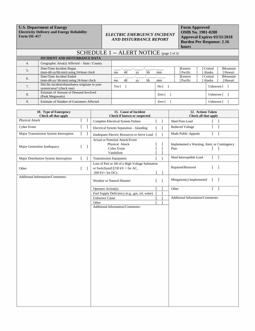
U.S. Department of Energy Electricity Delivery and Energy Reliability
Form OE-417 ELECTRIC EMERGENCY INCIDENT
AND DISTURBANCE REPORT
Form Approved
OMB No. 1901-0288
Approval Expires 03/31/2018
Burden Per Response: 2.16
hours
SCHEDULE 1 -- ALERT NOTICE (page 2 of 3) INCIDENT AND DISTURBANCE DATA
4. Geographic Area(s) Affected – State / County
5. Date/Time Incident Began (mm-dd-yy/hh:mm) using 24-hour clock
____ - _____ - _____ / _____: _____ [ ]Eastern [ ] Central [ ]Mountain mo dd yy hh mm [ ] Pacific [ ] Alaska [ ] Hawaii
6. Date/Time Incident Ended
(mm-dd-yy/ hh:mm) using 24-hour clock
_____ - _____ - _____ / _____: _____ [ ]Eastern [ ] Central [ ]Mountain
mo dd yy hh mm [ ] Pacific [ ] Alaska [ ] Hawaii
7. Did the incident/disturbance originate in your system/area? (check one)
Yes [ ] No [ ] Unknown [ ]
8. Estimate of Amount of Demand Involved
(Peak Megawatts) Zero [ ] Unknown [ ]
9. Estimate of Number of Customers Affected Zero [ ] Unknown [ ]
10. Type of Emergency
Check all that apply
11. Cause of Incident
Check if known or suspected
12. Actions Taken
Check all that apply
Physical Attack [ ] Complete Electrical System Failure [ ] Shed Firm Load [ ]
Cyber Event [ ] Electrical System Separation – Islanding [ ] Reduced Voltage [ ]
Major Transmission System Interruption [ ] Inadequate Electric Resources to Serve Load [ ] Made Public Appeals [ ]
Major Generation Inadequacy [ ]
Actual or Potential Attack/Event
Physical Attack [ ]
Cyber Event [ ]
Vandalism [ ]
Implemented a Warning, Alert, or Contingency
Plan [ ]
Major Distribution System Interruption [ ] Transmission Equipment [ ] Shed Interruptible Load [ ]
Other [ ]
Loss of Part or All of a High Voltage Substation
or Switchyard (230 kV + for AC,
200 kV+ for DC). [ ]
Repaired/Restored [ ]
Additional Information/Comments: Weather or Natural Disaster [ ] Mitigation(s) Implemented [ ]
Operator Action(s) [ ] Other [ ] Fuel Supply Deficiency (e.g., gas, oil, water) [ ]
Unknown Cause [ ] Additional Information/Comments: Other [ ]
Additional Information/Comments:

U.S. Department of Energy Electricity Delivery and Energy Reliability
Form OE-417 ELECTRIC EMERGENCY INCIDENT
AND DISTURBANCE REPORT
Form Approved
OMB No. 1901-0288
Approval Expires 03/31/2018
Burden Per Response: 2.16 hours
SCHEDULE 2 -- NARRATIVE DESCRIPTION (page 3 of 3)
Information on Schedule 2 will not be disclosed to the public to the extent that it satisfies the criteria for
exemption under the Freedom of Information Act, e.g., exemptions for confidential commercial information
and trade secrets or certain information that could endanger the physical safety of an individual.
NAME OF OFFICIAL THAT NEEDS TO BE CONTACTED FOR FOLLOW-UP AND ANY ADDITIONAL INFORMATION
13. Name
14. Title
15. Telephone Number ( )-( )-( )
16. FAX Number ( )-( )-( )
17. E-mail Address
Provide a description of the incident and actions taken to resolve it. Include as appropriate, the cause of the incident/disturbance,
change in frequency, mitigation actions taken, equipment damaged, critical infrastructures interrupted, effects on other systems, and
preliminary results from any investigations. Be sure to identify: the estimate restoration date, the name of any lost high voltage
substations or switchyards, whether there was any electrical system separation (and if there were, what the islanding boundaries were),
and the name of the generators and voltage lines that were lost (shown by capacity type and voltage size grouping). If necessary, copy
and attach additional sheets. Equivalent documents, containing this information can be supplied to meet the requirement; this includes the
NERC EOP-004 Disturbance Report. Along with the filing of Schedule 2, a final (updated) Schedule 1 needs to be filed. Check the Final
box on line 1 for Alert Status on Schedule 1 and submit this and the completed Schedule 2 no later than 72 hours after detection that a
criterion was met.
18. Narrative:
19. Estimated Restoration Date for all Affected Customers
Who Can Receive Power
_____ - _____ - _____
mo dd yy
20. Name of Assets Impacted