Review - Stanford University€¢ Sample exam questions to posted on website ... – Protein design ... – Even ab initio approaches usually take advantage of

Review

CS/CME/BioE/Biophys/BMI279Nov.30andDec.5,2017

RonDror

1

Information on the exam

• The exam will focus on high-level concepts – You may use two (single-sided) pages of notes, but the

emphasis is not on memorization of detail – You won’t be pressed for time

• Lecture slides (and homeworks) are a good way to review – Based on the mid-quarter survey, we’ve posted annotated

versions of the slides on the web page—but the main points are usually made explicitly on the lecture slides

– Homework solutions available in class (hard copies) • Sample exam questions to posted on website • In this lecture, I’ll review some of the most important

points and discuss recurring themes 2

Outline

• Atomic-level modeling of proteins and other macromolecules – Protein structure – Energy functions and their relationship to molecular conformation – Molecular dynamics simulation – Protein structure prediction – Protein design – Ligand docking

• Coarser-level modeling and imaging-based methods – Fourier transforms and convolution – Image analysis – X-ray crystallography – Single-particle electron microscopy – Microscopy – Diffusion and cellular-level simulation – Genome structure

• Recurring themes 3

Atomic-level modeling of proteins and other macromolecules

4

Protein Structure

5

Atomic-level modeling

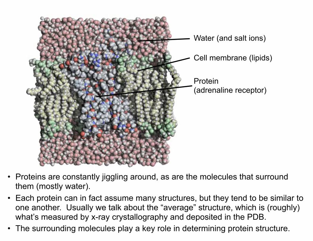
Water (and salt ions)

Protein (adrenaline receptor)

Cell membrane (lipids)

• Proteins are constantly jiggling around, as are the molecules that surround them (mostly water).

• Each protein can in fact assume many structures, but they tend to be similar to one another. Usually we talk about the “average” structure, which is (roughly) what’s measured by x-ray crystallography and deposited in the PDB.

• The surrounding molecules play a key role in determining protein structure.

Two-dimensional protein structure

• Proteins are chains of amino acids • These amino acids are identical except for their

sidechains (R groups in the diagram below). – Therefore proteins have regular (repeating) backbones

with differing side chains – The different side chains have different chemical

properties, and they ultimately determine the 3D structure of the protein.

7http://bcachemistry.wordpress.com/2014/05/28/chemical-bonds-in-spider-silk-and-venom/

What determines the three-dimensional structure of a protein?

• Basic interactions – Bond length stretching – Bond angle bending – Torsional angle twisting – Electrostatic interaction – Van der Waals interaction

• Complex interactions – Hydrogen bonds – Hydrophobic effect – These “complex interactions,” which result from the basic

interactions above, are particularly important to understanding why proteins adopt particular 3D structures

8

Energy functions and their relationship to molecular conformation

9


Potential energy functions

• A potential energy function U(x) specifies the total potential energy of a system of atoms as a function of all their positions (x) – For a system with n atoms, x is a vector of length 3n (x, y, and z

coordinates for every atom) – In the general case, include not only atoms in the protein but also

surrounding atoms (e.g., water) • The force on each atom can be computed by taking derivatives of

the potential energy function

10

Ene

rgy

(U)

Position

Ene

rgy

(U)

PositionPosition

Bonded terms

Non-bonded terms

Exampleofapotentialenergyfunction:molecularmechanicsforcefield

( )angles

20kθ θ θ+ −∑

i j

i j i ij

q qr>

+∑∑

12 6ij ij

i j i ij ij

A Br r>

+ −∑∑

Bond lengths (“Stretch”)

Bond angles (“Bend”)

Torsional/dihedral angles

Electrostatic

Van der Waals

U = kb b− b0( )2bonds∑

+ kφ ,n 1+ cos nφ −φn( )⎡⎣ ⎤⎦n∑

torsions∑

Aboveistheformofatypicalmolecularmechanicsforcefield(asusedinmoleculardynamicssimulations,forexample).Thetermscorrespondtothe“basicinteractions”discussedpreviously.

The Boltzmann Distribution

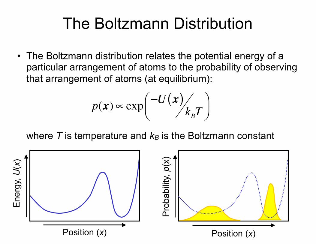
• The Boltzmann distribution relates the potential energy of a particular arrangement of atoms to the probability of observing that arrangement of atoms (at equilibrium):where T is temperature and kB is the Boltzmann constant

p(x)∝ exp −U x( )kBT

⎛⎝⎜

⎞⎠⎟

Ene

rgy,

U(x

)

Position (x)

Pro

babi

lity,

p(x

)

Position (x)

Macrostates• We typically care most about the probability that protein atoms

will be in some approximate arrangement, with any arrangement of surrounding atoms

• We thus care about the probability of sets of atomic arrangements, called macrostates – These correspond roughly to wells of the potential energy function – To calculate probability of a well, we sum the probabilities of all the

specific atomic arrangements it contains

13

Ene

rgy,

U(x

)

Position (x)

Pro

babi

lity,

p(x

)

Position (x)

Free energies• The free energy GA of a macrostate A satisfies:

• Clarifications: – Free energies are clearly defined only for macrostates – However, in protein structure prediction, protein design,

and ligand docking, it’s often useful to define a “free energy function” that approximates a free energy for some neighborhood of each arrangement of protein atoms • To predict protein structure, we minimize free energy, not

potential energy – The term “energy function” is used for both potential

energy and free energy functions14

P(A) = exp −GAkBT( )

Molecular dynamics simulation

15


Molecular dynamics (MD) simulation• An MD simulation predicts how atoms move around based on

physical models of their interactions • Of the atomic-level modeling techniques we covered, this is

closest to the physics; it attempts to predict the real dynamics of the system

• It can thus be used to capture functionally important processes, including structural changes in proteins, protein-ligand binding, or protein folding

16

Basic MD algorithm

• Step through time (very short steps) • At each time step, calculate force acting on every

atom using a molecular mechanics force field • Then update atom positions and velocities using

Newton’s second law

17

dxdt

= v

dvdt

=F x( )m

Note:thisisinherentlyanapproximation,becausewe’reusingclassicalphysicsratherthanquantummechanics.(Quantummechanicalcalculationsareusedtoparameterizeforcefields,however.)

MD is computationally intensive

• Because: – One needs to take millions to trillions of timesteps to get

to timescales on which events of interest take place – Computing the forces at each time step involves

substantial computation • Particularly for the non-bonded force terms, which act

between every pair of atoms

18

Sampling• Given enough time, an MD simulation will sample the full

Boltzmann distribution of the system – This means that if one took a snapshot from the simulation after

a long period of time, the probability of the atoms being in a particular arrangement is given by the Boltzmann distribution

• One can also sample the Boltzmann distribution in other ways, including Monte Carlo sampling with the Metropolis criterion – Metropolis Monte Carlo: generate moves at random. Accept any

move that decreases the energy. Accept moves that increase the energy by ∆U with probability

– If one decreases the temperature over time, this becomes a minimization method (simulated annealing) 19

e−ΔU

kBT

Protein structure prediction

20


Protein structure prediction

• The goal: given the amino acid sequence of a protein, predict its average three-dimensional structure

• In theory, one could do this by MD simulation, but that isn’t practical

• Practical methods for protein structure prediction take advantage of existing data on protein structure (and sequence)

21

Two main approaches to protein structure prediction

• Template-based modeling (homology modeling) – Used when one can identify one or more likely

homologs of known structure (usually the case) • Ab initio structure prediction

– Used when one cannot identify any likely homolog of known structure

– Even ab initio approaches usually take advantage of available structural data, but in more subtle ways

22

Template-based structure prediction: basic workflow

• User provides a query sequence with unknown structure

• Search the PDB for proteins with similar sequence and known structure. Pick the best match (the template).

• Build a model based on that template – One can also build a model based on multiple

templates, where different templates are used for different parts of the protein.

23

Principle underlying template-based modeling: structure is more conserved than sequence

• Proteins with similar sequences tend to be homologs, meaning that they evolved from a common ancestor

• The fold of the protein (i.e., its overall structure) tends to be conserved during evolution

• This tendency is very strong. Even proteins with 15% sequence identity usually have similar structures. – During evolution, sequence changes more quickly than

structure

24

Ab initio structure prediction (as exemplified by Rosetta)

• Search for structure that minimizes an energy function – This energy function is knowledge-based (informed, in particular,

by statistics of the PDB), and it approximates a free energy function

• Use a knowledge-based search strategy – Rosetta uses a Monte Carlo search method involving “fragment

assembly,” in which it tries replacing structures of small fragments of the protein with fragment structures found in the PDB

25

Proteinfoldinggame:letpeoplehelpwiththesearchprocess

Protein design

26


Protein design

• Goal: given a desired approximate three-dimensional structure (or structural characteristics), find an amino acid sequence that will fold to that structure

• In principle, we could do this by searching over sequences and doing ab initio structure prediction for each possible sequence, but that’s not practical

27

Simplifying the problem

• Instead of predicting the structure for each sequence considered, just focus on the desired structure, and find the sequence that minimizes its energy – Energy is generally measured by a knowledge-based

free energy function • Consider a discrete set of rotamers for each

amino acid side chain – Minimize simultaneously over identities and rotamers

of amino acids • Assume the backbone is fixed

– Or give it a bit of “wiggle room” 28

Heuristic but effective

• These simplifications mean that practical protein design methodologies are highly heuristic, but they’ve proven surprisingly effective

• The minimization problem itself is also usually solved with heuristic methods (e.g., Metropolis Monte Carlo)

29

Ligand docking

30


Ligand docking

• Goals: – Given a ligand known to bind a particular protein,

determine its binding pose (i.e., location, orientation, and internal conformation of the bound ligand)

– Determine how tightly a ligand binds a given protein

31

http://www.slideshare.net/baoilleach/proteinligand-docking-13581869

Binding affinity

• Binding affinity quantifies the binding strength of a ligand to a protein (or other target)

• Conceptual definition: if we mix the protein and the ligand (with no other ligands around), what fraction of the time will the protein have a ligand bound?

• Affinity can be expressed as the difference ΔG in free energy of the bound state and the unbound state, or as the concentration of unbound ligand molecules at which half the protein molecules will have a ligand bound

32

Docking is heuristic

• In principle, we could estimate binding affinity by measuring the fraction of time the ligand is bound in an MD simulation, but this isn’t practical

33

Docking methodology

• Ligand docking is a fast, heuristic approach with two key components – A scoring function that very roughly approximates the binding affinity

of a ligand to a protein given a binding pose – A search method that searches for the best-scoring binding pose for

a given ligand • Most ligand docking methods assume that

– The protein is rigid – The approximate binding site is known

• That is, one is looking for ligands that will bind to a particular site on the target

• In reality, ligand mobility, protein mobility, and water molecules all play a major role in determining binding affinity – Docking is approximate but useful – The term scoring function is used instead of energy function to

emphasize the highly approximate nature of the scoring function 34

• Some of these concepts apply with little or no modification to RNA and other biomolecules – Energy functions and their relationship to molecular

conformation – Molecular dynamics simulation – Ligand docking

• In other cases, the basic ideas apply, but the techniques are different – (RNA) structure prediction – (RNA) design

To what extent do these concepts apply to other biomolecules (e.g, RNA)?

RNA’ssecondarystructureisquitedifferentfromaprotein’s

Coarser-level modeling and imaging-based methods

36

Fourier transforms and convolution

37


Writing functions as sums of sinusoids• Given a function defined on an interval of length L, we can write it as

a sum of sinusoids with the following frequencies/periods: – Frequencies: 0, 1/L, 2/L, 3/L, …. – Periods: constant term, L, L/2, L/3, …

38

Originalfunction Sumofsinusoidsbelow

+ + +

DecreasingperiodIncreasingfrequency

+ +

Magnitude:0.39

+

• Each of these sinusoidal terms has a magnitude (scale factor) and a phase (shift).

Originalfunction Sumofsinusoidsbelow

Magnitude:1.9Phase:-.94

Magnitude:0.27Phase:-1.4 Phase:-2.8

Writing functions as sums of sinusoids

Magnitude:-0.3Phase:0(arbitrary)

• We can thus express the original function as a series of magnitude and phase coefficients – We can express each pair of magnitude and phase coefficients as a

complex number • The Fourier transform maps the function to this set of complex

numbers, providing an alternative representation of the function. • This also works for functions of 2 or 3 variables (e.g., images) • Fourier transforms can be computed efficiently using the Fast

Fourier Transform (FFT) algorithm

40

The Fourier Transform: Expressing a function as a set of sinusoidal term coefficients

Magnitude:0.39Magnitude:1.9Phase:-.94

Magnitude:0.27Phase:-1.4 Phase:-2.8

Magnitude:-0.3

Sinusoid1(periodL,frequency1/L)

Constantterm(frequency0)

Sinusoid2(periodL/2,frequency2/L)

Sinusoid3(periodL/3,frequency3/L)

Phase:0(arbitrary)

Convolution

• Convolution is a weighted moving average – To convolve one function with another, we computed a

weighted moving average of one function using the other function to specify the weights

41

f g fconvolvedwithg

Convolution = multiplication in frequency domain

• Convolving two functions is equivalent to multiplying them in the frequency domain

• In other words, we can perform a convolution by taking the Fourier transform of both functions, multiplying the results, and then performing an inverse Fourier transform

• Why is this important? – It provides an efficient way to perform large convolutions

(thanks to the FFT) – It allows us to interpret convolutions in terms of what they do

to different frequency components (e.g., high-pass and low-pass filters) 42

Image analysis

43


Representations of an image• We can think of a grayscale image

as: – A two-dimensional array of brightness

values – A function of two variables (x and y),

which returns the brightness of the pixel at position (x, y)

• A color image can be treated as: – Three separate images, one for each

color channel (red, green, blue) – A function that returns three values (red,

green, blue) for each (x, y) pair44

x

y

Reducing image noise

• We can reduce image noise using various filters (e.g., mean, median, Gaussian) – These all rely on the fact that nearby pixels in an image tend to

be similar • The mean and Gaussian filters (and many others) are

convolutions, and can thus be expressed as multiplications in the frequency domain – These denoising filters are low-pass filters. They reduce high-

frequency components while preserving low-frequency components

– These filters work because real images have mostly low-frequency content, while noise tends to have a lot of high-frequency content

45

High-pass filters

• A high-pass filter reduces low-frequency components while preserving high-frequency components

• We can sharpen images by adding a high-pass filtered version of the image to the original image

• High-pass filtering can also be used to remove undesired background brightness that varies smoothly across the image

46

Principal component analysis (PCA)• Basic idea: given a set of points in a multi-dimensional

space, we wish to find the linear subspace (line, plane, etc.) that best fits those points.

47

• PCA provides a way to represent high-dimensional data sets (such as images) approximately in just a few dimensions

• It is thus useful in summarization and classification of images

Firstprincipalcomponent

Secondprincipalcomponent

X-ray crystallography

48


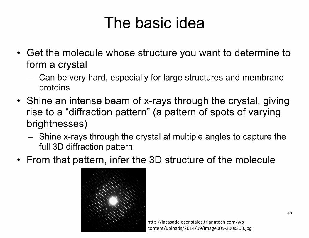
The basic idea

• Get the molecule whose structure you want to determine to form a crystal – Can be very hard, especially for large structures and membrane

proteins • Shine an intense beam of x-rays through the crystal, giving

rise to a “diffraction pattern” (a pattern of spots of varying brightnesses) – Shine x-rays through the crystal at multiple angles to capture the

full 3D diffraction pattern • From that pattern, infer the 3D structure of the molecule

49

http://lacasadeloscristales.trianatech.com/wp-content/uploads/2014/09/image005-300x300.jpg

How does the diffraction pattern relate to the molecular structure?

• The diffraction pattern is the Fourier transform of the electron density! – But only the magnitude of each Fourier coefficient is

measured, not the phase – The lack of phase information makes solving the

structure (i.e., going from the diffraction pattern to a set of 3D atomic coordinates) challenging

50

http://www.lynceantech.com/images/electron_density_map.png

Contourmapofelectrondensity

Solving for molecular structure

• Step 1: Initial phasing – Come up with an approximate solution for the structure

(and thus an approximate set of phases), often using a homologous protein as a model

• Step 2: Phase refinement – Search for perturbations that improve the fit to the

experimental data (the diffraction pattern), often using simulated annealing

– Restrain the search to “realistic” molecular structures, usually using a molecular mechanics force field

51

Single-particle electron microscopy

52


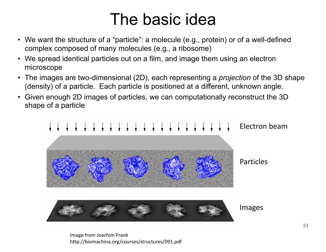
The basic idea• We want the structure of a “particle”: a molecule (e.g., protein) or of a well-defined

complex composed of many molecules (e.g., a ribosome) • We spread identical particles out on a film, and image them using an electron

microscope • The images are two-dimensional (2D), each representing a projection of the 3D shape

(density) of a particle. Each particle is positioned at a different, unknown angle. • Given enough 2D images of particles, we can computationally reconstruct the 3D

shape of a particle

53

ImagefromJoachimFrankhttp://biomachina.org/courses/structures/091.pdf

Electronbeam

Particles

Images

Determining the 3D structure: key steps

• 2D image analysis: First, go from raw image data to high-resolution 2D projections – Image preprocessing – Particle picking – Image clustering and class averaging: reduce image

noise by identifying images with similar view angles, aligning them, and averaging them

54ImagefromJoachimFrankhttp://biomachina.org/courses/structures/091.pdf

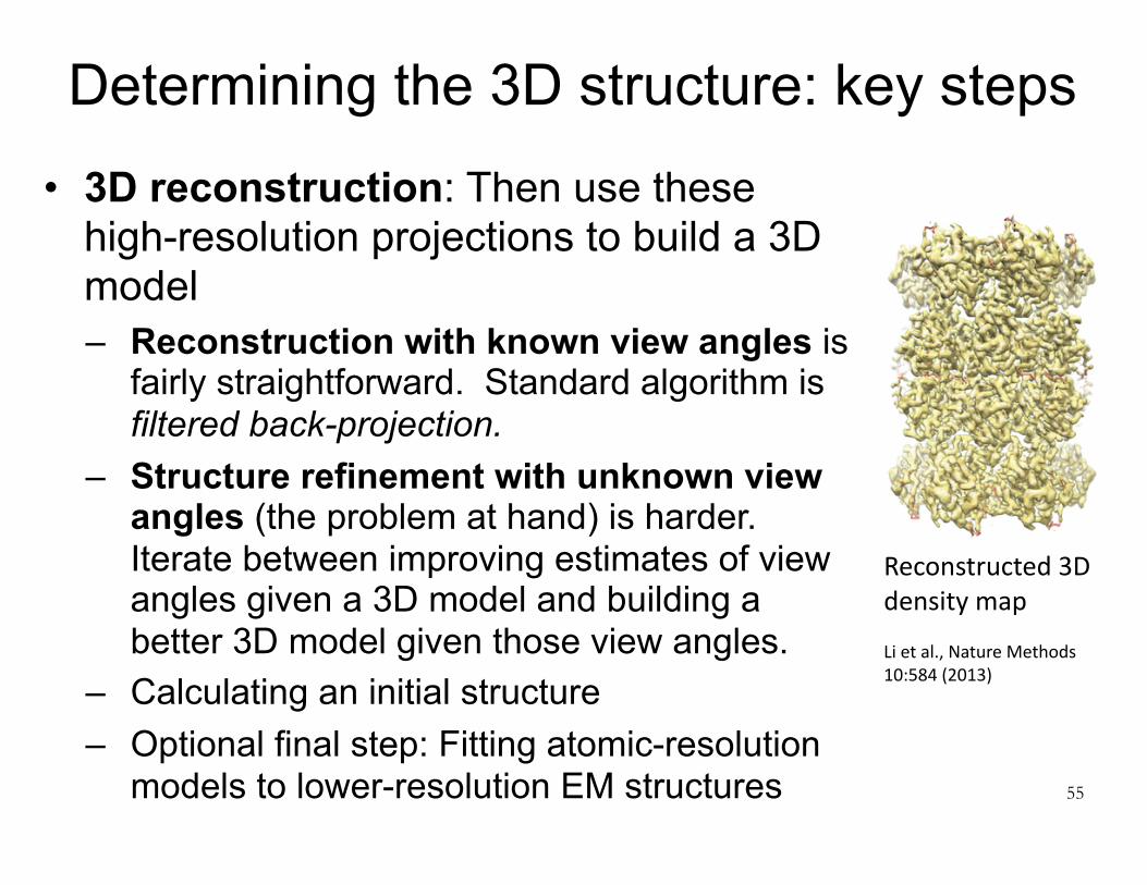
Determining the 3D structure: key steps

• 3D reconstruction: Then use these high-resolution projections to build a 3D model – Reconstruction with known view angles is

fairly straightforward. Standard algorithm is filtered back-projection.

– Structure refinement with unknown view angles (the problem at hand) is harder. Iterate between improving estimates of view angles given a 3D model and building a better 3D model given those view angles.

– Calculating an initial structure – Optional final step: Fitting atomic-resolution

models to lower-resolution EM structures 55

Reconstructed3Ddensitymap

Lietal.,NatureMethods10:584(2013)

Microscopy

56


Fluorescence microscopy: basic idea

• Suppose we want to know where a particular type of protein is located in the cell, or how these proteins move around

• We can’t do this by simply looking through a microscope, because: – We (usually) don’t have sufficient resolution – The protein of interest doesn’t look different from those

around it • Solution: Make the molecules of interest glow by

attachment of fluorophores (fluorescent molecules) – When you shine light of a particular wavelength on a

fluorophore, it emits light of a different wavelength 57

Single-molecule tracking• If the density of fluorescent molecules is sufficiently

low, we can track individual molecules – Doing this well is a challenging computational problem

Data:BettinavanLengerich,NataliaJuraTrackingandmovie:RobinJia

58

The diffraction limit

• The image observed under a microscope is always slightly blurred due to fundamental limitations on how well a lens can focus light – The observed image is a low-pass filtered version of

the ideal image • This leads to a limit on resolution known as the

diffraction limit – The achievable resolution scales with wavelength of

the radiation used (i.e., a shorter wavelength leads to a smaller minimum distance between resolvable points)

– X-rays have shorter wavelength than visible light. Electrons have much shorter wavelengths. 59

Diffusion and cellular-level simulation

60


How do molecules move within a cell?

• Molecules jiggle about because other molecules keep bumping into them

• Individual molecules thus follow a random walk • Diffusion = many random walks by many molecules

– Substance goes from region of high concentration to region of lower concentration

– Aggregate behavior is deterministic61

From Inner Life of the Cell | Protein Packing, XVIVO and Biovisions @ Harvard

https://www.youtube.com/watch?v=1jYabtziQZo

Particle-based perspective

• In the basic case of random, unconfined, undirected motion: – Individual molecules follow a random walk, leading to

Brownian motion – Mean squared displacement is proportional to time – The proportionality constant is specified by the

diffusion constant • Faster-moving molecules have larger diffusion constants

62

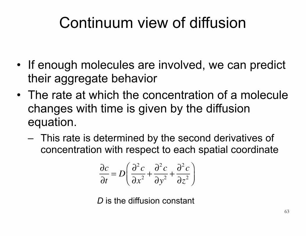
Continuum view of diffusion

• If enough molecules are involved, we can predict their aggregate behavior

• The rate at which the concentration of a molecule changes with time is given by the diffusion equation. – This rate is determined by the second derivatives of

concentration with respect to each spatial coordinate

63

∂c∂t

= D ∂2c∂x2

+ ∂2c∂y2

+ ∂2c∂z2

⎛⎝⎜

⎞⎠⎟

D is the diffusion constant

Reaction-diffusion simulation

• A common way to model how molecules move within the cell involves reaction-diffusion simulation

• Basic rules: – Molecular move around by diffusion – When two molecules come close together, they have

some probability of reacting to combine or modify one another

• Two implementation strategies: – Particle-based models – Continuum models

(based on the diffusion equation) 64

Genome structure

65


10 bp

100 bp

1 Kbp

10 Kbp

100 Kbp

1 Mbp

10 Mbp

100 Mbp

Genomeorganizationisstudiedatmultiplescales

4)Wholechromosomes

3)Loopsanddomains

2)Chromatin

1)DNA

bp = base pair. Usually one writes “1 Mb” instead of “1 MBp”, etc.

Note:the“30-nmfiber”isobservedinvitrobutmaynotexistinvivo(andwon’tappearonthefinal!)

FromAdrianSanbornandhttps://www.slideshare.net/vjcummins/chromosome-structure-v2

DNA structure

• At the scale of protein structure, DNA forms just a single dominant structure: the double helix – DNA primarily stores information, in contrast to proteins,

which act as molecular machines • On scales of hundreds of base pairs (bp), DNA wraps

around histone proteins, forming nucleosomes – Strings of nucleosomes are called chromatin

• On scales of 10 Kbp or greater, chromatin has a complicated, dynamic structure – This has a big effect on gene expression – It’s a focus of current research

67

#ofPicturesTogether

SIMPSONS CONTACT MAP

ChromosomeconformationcapturetechniquesidentifyfrequenciesofcontactsbetweenonepartofaDNAstrandandanother.Thesecontactfrequenciescanbeusedtoinferstructuralfeaturesofchromatin,suchasdomainsandloops.

FromErezLieberman-Aiden

Simulating chromatin’s spatial organization

• Simulations are used: – To reconstruct 3D genome structure, beginning with a contact

map. Here, the contact map is used as a set of constraints. – To test mechanistic hypotheses (e.g., for how loops and domains

are formed). One generally compares the results to experimental contact maps.

• Multiple scales – The simulations above are coarse-grained, with one particle

representing 1-500 Kbp (closer to 1 Kbp for simulation of loops/domains, closer to 500 Kbp for simulation of whole chromosomes)

– Simulations are also used to study DNA structure on finer scales. These might be all-atom MD simulations (one particle represents one atom), or they might be somewhat coarser grained (e.g., one particle represents one base).

Recurring Themes

70

Physics-based vs. data-driven approaches

• Physics-based approaches: modeling based on first-principles physics

• Data-driven approaches: inference/learning based on experimental data

• Examples: – Physics-based vs. knowledge-based energy functions – Molecular dynamics vs. protein structure prediction

• Most methods fall somewhere on the continuum between these two extremes – Examples: ligand docking or solving x-ray crystal

structures 71

Energy functions

• Energy functions (representing either potential energy or free energy) play a key role in many of the techniques we’ve covered, including: – Molecular dynamics – Protein structure prediction – Protein design – Ligand docking – X-ray crystallography

72

Both structural interpretation of experimental data and structural predictions require computation

• Structural predictions – Protein structure prediction – Molecular dynamics simulation – Ligand docking – Reaction-diffusion simulations

• Structural interpretation of experimental data – X-ray crystallography – Single-particle electron microscopy – Image analysis for fluorescence microscopy data – Analyzing chromosome conformation capture data

73

Recurring math concepts

• Fourier transforms and convolution play important roles in: – Image analysis – X-ray crystallography – Single-particle electron microscopy – (And also in molecular dynamics and some docking

methods, though you’re not responsible for that) • Another recurring math concept: Monte Carlo

methods

74

Similarities and differences in methods employed at different spatial scales

• Atomic-level modeling of single proteins vs. coarser-level modeling of complexes and cells

• Experimental methods: x-ray crystallography vs. single-particle electron microscopy

• Simulation methods: molecular dynamics vs. reaction-diffusion simulations

75

How did people do these things before they had powerful computers?

76

Large-scale simulation in 1971• Excerpt from “Protein synthesis: an epic on the cellular level” • Performed at Stanford!

77

https://www.youtube.com/watch?v=u9dhO0iCLww

Next quarter: CS/CME/Biophys/BMI 371 “Computational biology in four dimensions”

• I’m teaching a course next quarter that complements this one

• Similar topic area, but with a focus on current cutting-edge research – Focus is on reading, presentation, discussion, and

critique of published papers

78

Course evaluations

• Please fill them out

79

Documents

Review - Stanford University€¢ Sample exam questions to posted on website ... – Protein design ... – Even ab initio approaches usually take advantage of