Review. Review of Standard Errors (cont.) Problem: we do not know 2 Solution: estimate 2 We do not observe the ACTUAL error terms, i We DO observe

Review

0 1 1

2

( ) 0

( )

( , ) 0

Gauss–Markov DGP

, if

's fixed across samples.

i i i

i

i

i j

Y X

E

Var

Cov i j

X

Review of Standard Errors (cont.)

• Problem: we do not know 2

• Solution: estimate 2

• We do not observe the ACTUAL error terms, i

• We DO observe the residual, ei

s2

ei2

n k 1

Review of Standard Errors (cont.)

• Our formula for Estimated Standard Errors relied on ALL the Gauss–Markov DGP assumptions.

• For this lecture, we will focus on the assumption of homoskedasticity.

• What happens if we relax the assumption that ?Var(i ) 2

Heteroskedasticity (Chapter 10.1)

• HETEROSKEDASTICITY

– The variance of i is NOT a constant 2.

– The variance of i is greater for some observations than for others.

Var(i ) i2

Heteroskedasticity (cont.)

• For example, consider a regression of housing expenditures on income.

• Consumers with low values of income have little scope for varying their rent expenditures. Var(i ) is low.

• Wealthy consumers can choose to spend a lot of money on rent, or to spend less, depending on tastes. Var(i ) is high.

Renti

0

1Income

i

i

Figure 10.1 Rents and Incomes for a Sample of New Yorkers

OLS and Heteroskedasticity

• What are the implications of heteroskedasticity for OLS?

• Under the Gauss–Markov assumptions (including homoskedasticity), OLS was the Best Linear Unbiased Estimator.

• Under heteroskedasticity, is OLS still Unbiased?

• Is OLS still Best?

OLS and Heteroskedasticity (cont.)

• A DGP with Heteroskedasticity

0 1 1

2

...

( ) 0

( )

( , ) 0

’s fixed across samples

i i k ki i

i

i i

i j

Y X X

E

Var

Cov for i j

X


• The unbiasedness conditions are the same as under the Gauss–Markov DGP.

• OLS is still unbiased!


• To determine whether OLS is “Best” (i.e. the unbiased linear estimator with the lowest variance), we need to calculate the variance of a linear estimator under heteroskedasticity.

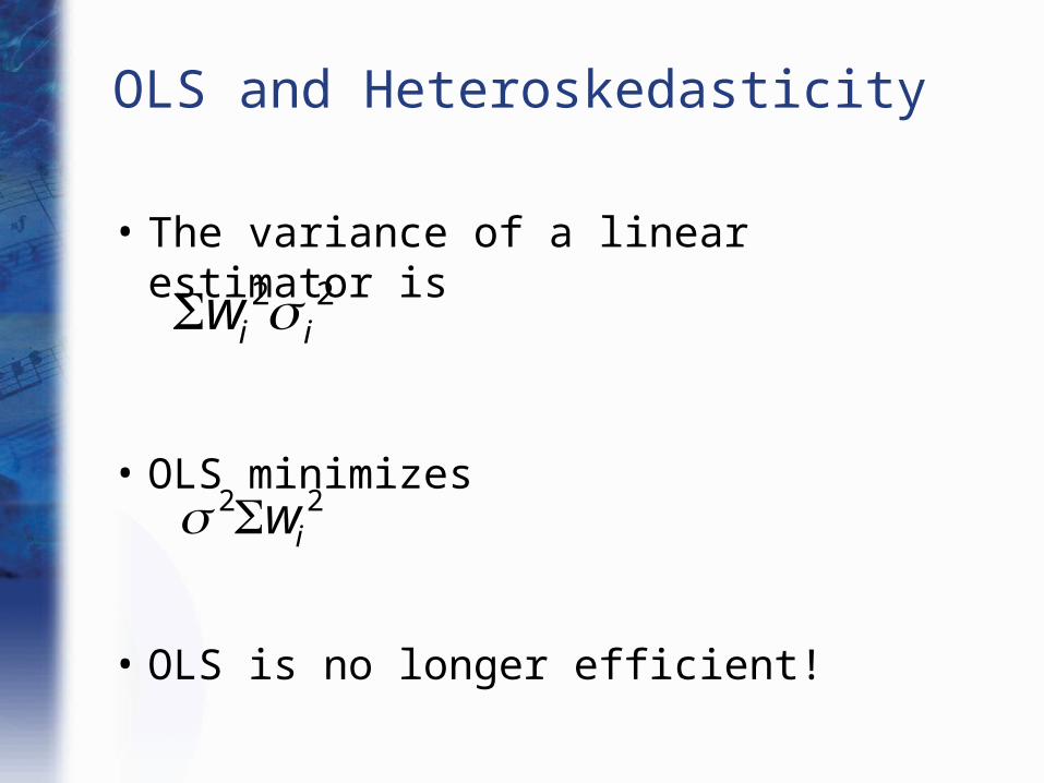
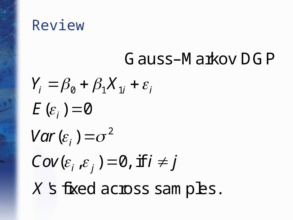
2 2i iw

2 2iw

OLS and Heteroskedasticity

• The variance of a linear estimator is

• OLS minimizes

• OLS is no longer efficient!


• Under heteroskedasticity, OLS is unbiased but inefficient.

• OLS does not have the smallest possible variance, but its variance may be acceptable. And the estimates are still unbiased.

• However, we do have one very serious problem: our estimated standard error formulas are wrong!


• Implications of Heteroskedasticity:

–OLS is still unbiased.

–OLS is no longer efficient; some other linear estimator will have a lower variance.

– Estimated Standard Errors will be incorrect; C.I.’s and hypothesis tests (both t- and F- tests) will be incorrect.


• Implications of Heteroskedasticity

–OLS is no longer efficient; some other linear estimator will have a lower variance.•Can we use a better estimator?

– Estimated Standard Errors will be incorrect; C.I.’s and hypothesis tests (both t- and F- tests) will be incorrect.• If we keep using OLS, can we calculate

correct e.s.e.’s?

Tests for Heteroskedasticity

• Before we turn to remedies for heteroskedasticity, let us first consider tests for the complication.

• There are two types of tests:

1. Tests for continuous changes in variance: White and Breusch–Pagan tests

2. Tests for discrete (lumpy) changes in variance: the Goldfeld–Quandt test

The White Test

• The White test for heteroskedasticity has a basic premise: if disturbances are homoskedastic, then squared errors are on average roughly constant.

• Explanators should NOT be able to predict squared errors, or their proxy, squared residuals.

• The White test is the most general test for heteroskedasticity.

The White Test (cont.)

• Five Steps of the White Test:

1. Regress Y against your various explanators using OLS

2. Compute the OLS residuals, e1...en

3. Regress ei2 against a constant, all of

the explanators, the squares of the explanators, and all possible interactions between the explanators (p slopes total)

The White Test (cont.)

• Five Steps of the White Test (cont.)

4. Compute R2 from the “auxilliary equation” in step 3

5. Compare nR2 to the critical value from the Chi-squared distribution with p degrees of freedom.

The White Test: Example

0 1 2 3

0 1 2 3

2 2 20 1 2 3 4

25 6 7

exp

ˆ ˆ ˆ ˆexp

exp exp

exp

i(1) Estimate Wage

(2) Calculate

(3) Regress

i i i i

i i i i i

i i i i

i i i i

ed IQ

e Wage ed IQ

e ed ed

IQ IQ ed

8 9

2

2

exp

9 16.92

(4) Compute from (3)

(5) Reject homoskedasticity if Chi-Squared critical

value with degrees of freedom ( , if the

significa

i i i i ied IQ IQ v

nR

nR

0.05nce level is )

The White Test

• The White test is very general, and provides very explicit directions. The econometrician has no judgment calls to make.

• The White test also burns through degrees of freedom very, very rapidly.

• The White test is appropriate only for “large” sample sizes.

The Breusch–Pagan Test

• The Breusch–Pagan test is very similar to the White test.

• The White test specifies exactly which explanators to include in the auxilliary equation. Because the test includes cross-terms, the number of slopes (p) increases very quickly.

• In the Breusch–Pagan test, the econometrician selects which explanators to include. Otherwise, the tests are the same.

The Breusch–Pagan Test (cont.)

• In the Breusch–Pagan test, the econometrician selects m explanators to include in the auxilliary equation.

• Which explanators to include is a judgment call.

• A good judgment call leads to a more powerful test than the White test.

• A poor judgment call leads to a poor test.

The Goldfeld–Quandt Test

• Both the White test and the Breusch–Pagan test focus on smoothly changing variances for the disturbances.

• The Goldfeld–Quandt test compares the variance of error terms across discrete subgroups.

• Under homoskedasticity, all subgroups should have the same estimated variances.

The Goldfeld–Quandt Test (cont.)

• The Goldfeld–Quandt test compares the variance of error terms across discrete subgroups.

• The econometrician must divide the data into h discrete subgroups.


• If the Goldfeld–Quandt test is appropriate, it will generally be clear which subgroups to use.


• For example, the econometrician might ask whether men and women’s incomes vary similarly around their predicted means, given education and experience.

• To conduct a Goldfeld–Quandt test, divide the data into h = 2 groups, one for men and one for women.


(1) Divide the n observations into h groups, of sizes n1..n

h

(2) Choose two groups, say 1 and 2.

H0

:12

22 against H

a:

12

22

(3) Regress Y against the explanators for group 1.

(4) Regress Y against the explanators for group 2.

Goldfeld–Quandt Test (cont.)

(5) Relabel the groups as L and S, such that SSR

L

nL k

SSR

S

nS k

Compute G

SSRL

nL k

SSRS

nS k

(6) Compare G to the critical value for an F-statistic

with (nL k) and (n

S k) degrees of freedom.

Goldfeld–Quandt Test: An Example

• Do men and women’s incomes vary similarly about their respective means, given education and experience?

• That is, do the error terms for an income equation have different variances for men and women?

• We have a sample with 3,394 men and 3,146 women.

(1) Divide the n observations into men and women,

of sizes nm and n

w.

(2) We have only two groups, so choose both of them.

H0

:m

2 w

2 against Ha

:m

2 w

2

(3) For the men, regress

log(income)i

0

1ed

i

2exp

i

3exp

i2

i

(4) For the women, regress

log(income)i

0

1ed

i

2exp

i

3exp

i2 v

i

Goldfeld–Quandt Test: An Example (cont.)

Goldfeld–Quandt Test: An Example (cont.)

(5) sm

2 SSR

m

nm k

1736.64

3394 - 40.5123

sw

2 SSR

w

nw k

1851.52

3146 - 40.5893

Compute G 0.5893

0.51231.15

(6) Compare G to the critical value for an F-statistic

with 3142 and 3390 degrees of freedom, which is

0.99997 for the 5% significance level.

We reject the null hypothesis at the 5% level.

WHAT TO DO?

1. Sometimes logging the variables can solve the problem. Sometimes not.2. Use Generalized Least Squares to estimate the model with heteroscedasticity.

Generalized Least Squares

• OLS is unbiased, but not efficient.

• The OLS weights are not optimal.

• Suppose we are estimating a straight line through the origin:

• Under homoskedasticity, observations with higher X values are relatively less distorted by the error term.

• OLS places greater weight on observations with high X values.

Y X

Figure 10.2 Homoskedastic Disturbances More Misleading at Smaller X ’s


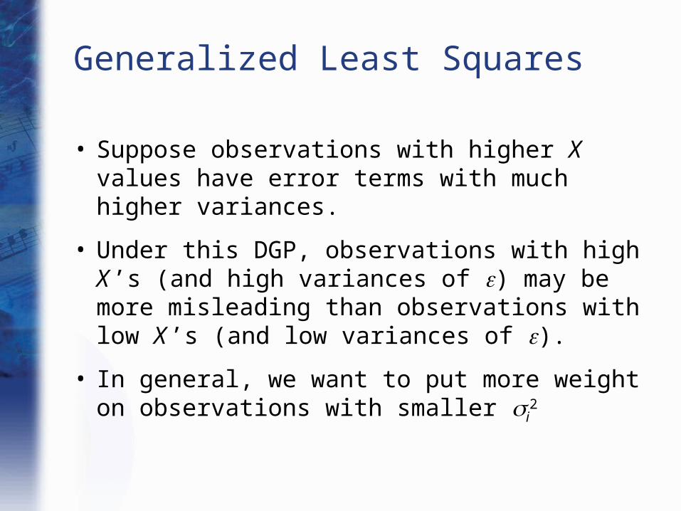
• Suppose observations with higher X values have error terms with much higher variances.

• Under this DGP, observations with high X ’s (and high variances of ) may be more misleading than observations with low X ’s (and low variances of ).

• In general, we want to put more weight on observations with smaller i

2

Heteroskedasticity with Smaller Disturbances at Smaller X ’s


• To construct the BLUE Estimator for S, we follow the same steps as before, but with our new variance formula. The resulting estimator is “Generalized Least Squares.”

Start with a linear estimator, wiY

i

Impose the unbiasedness conditions,

wiX

Ri0 for R S , w

iX

Si1

Find wi to minimize w

i2

i2

Generalized Least Squares (cont.)

• In practice, econometricians choose a different method for implementing GLS.

• Historically, it was computationally difficult to program a new estimator (with its own weights) for every different dataset.

• It was easier to re-weight the data first, and THEN apply the OLS estimator.


• We want to transform the data so that it is homoskedastic. Then we can apply OLS.

• It is convenient to rewrite the variance term of the heteroskedastic DGP as

Var(i ) 2di2


• If we know the di factor for each observation, we can transform the data by dividing through by di.

• Once we divide all variables by di, we obtain a new dataset that meets the Gauss–Markov conditions.

0 1

2 2 22 2

1

0

1 1

1, ( , ) 0

fixed across samples.

i i i

i i i i

i

i

ii i

i i i

jii j

i j i j

i

i

Y X

d d d d

Ed

Var Var dd d d

Cov Covd d d d

X

d

GLS: DGP for Transformed Data


• This procedure, Generalized Least Squares, has two steps:

1. Divide all variables by di

2. Apply OLS to the transformed variables

• This procedure optimally weights down observations with high di’s

• GLS is unbiased and efficient


• Note: we derive the same BLUE Estimator (Generalized Least Squares) whether we:

1. Find the optimal weights for heteroskedastic data, or

2. Transform the data to be homoskedastic, then use OLS weights

GLS: An Example

• We can solve heteroskedasticity by dividing our variables through by di.

• The DGP with the transformed data is Gauss–Markov.

• The catch: we don’t observe di. How can we implement this strategy in practice?

GLS: An Example (cont.)

• We want to estimate the relationship

• We are concerned that higher income individuals are less constrained in how much income they spend in rent. Lower income individuals cram into what housing they can afford; higher income individuals find housing to suit their needs/tastes.

• That is, Var(i ) may vary with income.

renti 0 1incomei i


• An initial guess:

• di = incomei

• If we have modeled heteroskedasticity correctly, then the BLUE Estimator is:

rent

income i

0

1

incomei

1 v

i

Var(i ) 2 ·incomei2

TABLE 10.1 Rent and Income in New York

TABLE 10.5 Estimating a Transformed Rent–Income Relationship, var(

i) 2 X

i2

Checking Understanding

• An initial guess:

• di = incomei

• How can we test to see if we have correctly modeled the heteroskedasticity?

rent

income i

0

1

incomei

1 v

i


Checking Understanding

• If we have the correct model of heteroskedasticity, then OLS with the transformed data should be homoskedastic.

• We can apply either a White test or a Breusch–Pagan test for heteroskedasticity to the model with the transformed data.

rent

income i

0

1

incomei

1 v

i

ei

0

1

1

incomei

2

1

incomei2

i

Checking Understanding (cont.)

• To run the White test, we regress

• nR2 = 7.17

• The critical value at the 0.05 significance level for a Chi-square statistic with 2 degrees of freedom is 5.99

• We reject the null hypothesis.

GLS: An Example

• Our initial guess:

• This guess didn’t do very well. Can we do better?

• Instead of blindly guessing, let’s try looking at the data first.


Figure 10.4 The Rent–Income Ratio Plotted Against the Inverse of Income

GLS: An Example

• We seem to have overcorrected for heteroskedasticity.

• Let’s try

rent

income i

0

1

income i

1

incomei v

i

Var(i ) 2 ·incomei

TABLE 10.6 Estimating a Second Transformed Rent–Income Relationship, var(i ) 2 Xi

GLS: An Example

• Unthinking application of the White test procedures for the transformed data leads to

• The interaction term reduces to a constant, which we already have in the auxilliary equation, so we omit it and use only the first 4 explanators.

0 1 2 3

4 5

1 1

1

ii i

i ii

e incomeincomeincome

income incomeincome


• nR2 = 6.16

• The critical value at the 0.05 significance level for a Chi-squared statistic with 4 degrees of freedom is 9.49

• We fail to reject the null hypothesis that the transformed data are homoskedastic.

• Warning: failing to reject a null hypothesis does NOT mean we can “accept” it.


• Generalized Least Squares is not trivial to apply in practice.

• Figuring out a reasonable di can be quite difficult.

• Next time we will learn another approach to constructing di , Feasible Generalized Least Squares.

Review

• In this lecture, we began relaxing the Gauss–Markov assumptions, starting with the assumption of homoskedasticity.

• Under heteroskedasticity, – OLS is still unbiased

– OLS is no longer efficient

– OLS e.s.e.’s are incorrect, so C.I., t-, and F- statistics are incorrect

Var(i ) 2di

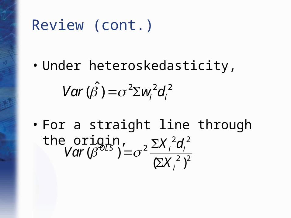
Review (cont.)

• Under heteroskedasticity,

• For a straight line through the origin,

2 2 2ˆ( ) i iVar w d

2 22

2 2ˆ( )

( )OLS i i

i

X dVar

X

Review (cont.)

• We can use squared residuals to test for heteroskedasticity.

• In the White test, we regress the squared residuals against all explanators, squares of explanators, and interactions of explanators. The nR2 of the auxilliary equation is distributed Chi-squared.

Review (cont.)

• The Breusch–Pagan test is similar, but the econometrician chooses the explanators for the auxilliary equation.

Review (cont.)

• In the Goldfeld–Quandt test, we first divide the data into distinct groups, and conduct our OLS regression on each group separately.

• We then estimate s2 for each group.

• The ratio of two s2 estimates is distributed as an F-statistic.

Review (cont.)

• Under heteroskedasticity, the BLUE Estimator is Generalized Least Squares

• To implement GLS:1. Divide all variables by di

2. Perform OLS on the transformed variables

• If we have used the correct di , the transformed data are homoskedastic. We can test this property.

Documents

Review. Review of Standard Errors (cont.) Problem: we do not know 2 Solution: estimate 2 We do not observe the ACTUAL error terms, i We DO observe