Nuclear SafetyNEA/CSNI/R(2016)4February 2016www.oecd-nea.org

Review of Uncertainty Methods for Computational Fluid Dynamics Application to Nuclear Reactor Thermal Hydraulics

Unclassified NEA/CSNI/R(2016)4 Organisation de Coopération et de Développement Économiques Organisation for Economic Co-operation and Development ___________________________________________________________________________________________

English text only NUCLEAR ENERGY AGENCY COMMITTEE ON THE SAFETY OF NUCLEAR INSTALLATIONS

Review of Uncertainty Methods for Computational Fluid Dynamics Application to Nuclear Reactor Thermal Hydraulics

Complete document available on OLIS in its original format This document and any map included herein are without prejudice to the status of or sovereignty over any territory, to the delimitation of international frontiers and boundaries and to the name of any territory, city or area.

NEA

/CSN

I/R(2016)4

Unclassified

English text only

2

ORGANISATION FOR ECONOMIC CO-OPERATION AND DEVELOPMENT The OECD is a unique forum where the governments of 34 democracies work together to address the economic, social and environmental challenges of globalisation. The OECD is also at the forefront of efforts to understand and to help governments respond to new developments and concerns, such as corporate governance, the information economy and the challenges of an ageing population. The Organisation provides a setting where governments can compare policy experiences, seek answers to common problems, identify good practice and work to co-ordinate domestic and international policies.

The OECD member countries are: Australia, Austria, Belgium, Canada, Chile, the Czech Republic, Denmark, Estonia, Finland, France, Germany, Greece, Hungary, Iceland, Ireland, Israel, Italy, Japan, Luxembourg, Mexico, the Netherlands, New Zealand, Norway, Poland, Portugal, the Republic of Korea, the Slovak Republic, Slovenia, Spain, Sweden, Switzerland, Turkey, the United Kingdom and the United States. The European Commission takes part in the work of the OECD.

OECD Publishing disseminates widely the results of the Organisation’s statistics gathering and research on economic, social and environmental issues, as well as the conventions, guidelines and standards agreed by its members.

NUCLEAR ENERGY AGENCY The OECD Nuclear Energy Agency (NEA) was established on 1 February 1958. Current NEA membership consists of

31 countries: Australia, Austria, Belgium, Canada, the Czech Republic, Denmark, Finland, France, Germany, Greece, Hungary, Iceland, Ireland, Italy, Japan, Korea, Luxembourg, Mexico, the Netherlands, Norway, Poland, Portugal, Russia, the Slovak Republic, Slovenia, Spain, Sweden, Switzerland, Turkey, the United Kingdom and the United States. The European Commission also takes part in the work of the Agency.

The mission of the NEA is:

– to assist its member countries in maintaining and further developing, through international co-operation, the scientific, technological and legal bases required for a safe, environmentally friendly and economical use of nuclear energy for peaceful purposes;

– to provide authoritative assessments and to forge common understandings on key issues, as input to government decisions on nuclear energy policy and to broader OECD policy analyses in areas such as energy and sustainable development.

Specific areas of competence of the NEA include the safety and regulation of nuclear activities, radioactive waste management, radiological protection, nuclear science, economic and technical analyses of the nuclear fuel cycle, nuclear law and liability, and public information.

The NEA Data Bank provides nuclear data and computer program services for participating countries. In these and related tasks, the NEA works in close collaboration with the International Atomic Energy Agency in Vienna, with which it has a Co-operation Agreement, as well as with other international organisations in the nuclear field.

This document and any map included herein are without prejudice to the status of or sovereignty over any territory, to the delimitation of international frontiers and boundaries and to the name of any territory, city or area.

Corrigenda to OECD publications may be found online at: www.oecd.org/publishing/corrigenda.

© OECD 2016

You can copy, download or print OECD content for your own use, and you can include excerpts from OECD publications, databases and multimedia products in your own documents, presentations, blogs, websites and teaching materials, provided that suitable acknowledgment of the OECD as source and copyright owner is given. All requests for public or commercial use and translation rights should be submitted to rights@oecd.org. Requests for permission to photocopy portions of this material for public or commercial use shall be addressed directly to the Copyright Clearance Center (CCC) at info@copyright.com or the Centre français d'exploitation du droit de copie (CFC) contact@cfcopies.com.

3

COMMITTEE ON THE SAFETY OF NUCLEAR INSTALLATIONS

The NEA Committee on the Safety of Nuclear Installations (CSNI) is an international committee made up of senior scientists and engineers with broad responsibilities for safety technology and research programmes, as well as representatives from regulatory authorities. It was created in 1973 to develop and co-ordinate the activities of the NEA concerning the technical aspects of the design, construction and operation of nuclear installations insofar as they affect the safety of such installations.

The committee’s purpose is to foster international co-operation in nuclear safety among NEA member countries. The main tasks of the CSNI are to exchange technical information and to promote collaboration between research, development, engineering and regulatory organisations; to review operating experience and the state of knowledge on selected topics of nuclear safety technology and safety assessment; to initiate and conduct programmes to overcome discrepancies, develop improvements and reach consensus on technical issues; and to promote the co-ordination of work that serves to maintain competence in nuclear safety matters, including the establishment of joint undertakings.

The priority of the CSNI is on the safety of nuclear installations and the design and construction of new reactors and installations. For advanced reactor designs, the committee provides a forum for improving safety-related knowledge and a vehicle for joint research.

In implementing its programme, the CSNI establishes co-operative mechanisms with the NEA Committee on Nuclear Regulatory Activities (CNRA), which is responsible for issues concerning the regulation, licensing and inspection of nuclear installations with regard to safety. It also co-operates with other NEA Standing Technical Committees, as well as with key international organisations such as the International Atomic Energy Agency (IAEA), on matters of common interest.

4

5

ACKNOWLEDGEMENTS

This report was prepared by D. Bestion (CEA, France), A. de Crécy (CEA, France), R. Camy (EDF, France), A. Barthet (EDF, France), S. Bellet (EDF, France), A. Badillo (PSI, Switzerland), B. Niceno (PSI, Switzerland), P. Hedberg (SSM, Sweden), J.L. Muñoz Cobo (UPV, Spain), F. Moretti (GRNSPG, Italy), M. Scheuerer (GRS, Germany), A. Nickolaeva (OKB Guidropress, Russia). The NEA official supporting the task was M.P. Kissane.

6

7

TABLE OF CONTENTS

Executive summary ......................................................................................................................................... 9

1. Introduction ............................................................................................................................................... 14

2. The domain of possible application of single-phase CFD for NRS .......................................................... 16

3. Links between PIRT, scaling, verification, validation and uncertainty quantification .............................. 20

3.1 Solving a complex reactor thermal-hydraulic issue .......................................................................... 20

3.2 Phenomena identification and ranking table ..................................................................................... 21

3.3 Scaling .............................................................................................................................................. 22

3.4 Verification and validation ............................................................................................................... 23

3.5 Uncertainty quantification ................................................................................................................ 24

3.6 Reassembling uncertainties .............................................................................................................. 25

4. Sources of uncertainty in LWR thermal-hydraulic simulations ................................................................ 26

4.1 The various sources of uncertainty in CFD applications to LWR .................................................... 26

4.2 Differences between system codes and single-phase CFD codes with respect to uncertainty ......... 28

5. Classification of methods for uncertainty quantification........................................................................... 30

5.1 Methods based on propagation of uncertainties ............................................................................... 30

5.2 Accuracy extrapolation methods ...................................................................................................... 31

5.3 The ASME V&V20 .......................................................................................................................... 31

5.4 Comparison of methods .................................................................................................................... 32

5.5 The role of validation in SETs and IETs/CETs in the UQ process .................................................. 32

6. An uncertainty propagation method extended to CFD .............................................................................. 34

6.1 Short description of the method ........................................................................................................ 34

6.2 Categorical variables and their treatment ......................................................................................... 34

6.3 An application case: “The heating floor” ......................................................................................... 36

6.4 Conclusions regarding the method ................................................................................................... 42

6.5 Characteristics of the method ........................................................................................................... 43

7. UMAE method applied to CFD ................................................................................................................. 43

7.1 Brief description of UMAE .............................................................................................................. 44

7.2 Short description of CIAU ................................................................................................................ 47

7.3 Towards a UMAE-CIAU-like approach to CFD UQ ....................................................................... 50

7.4 Characteristics of the method ........................................................................................................... 52

8

8. Summary of the asme method ................................................................................................................... 54

8.1 Characteristics of the method ........................................................................................................... 56

9. Uncertainty quantification using the deterministic sampling method ....................................................... 57

9.1 Statistical moments ........................................................................................................................... 57

9.2 A one-parameter example ................................................................................................................. 58

9.3 Inverse uncertainty quantification .................................................................................................... 61

9.4 Summary ........................................................................................................................................... 62

9.5 Characteristics of the DS method ..................................................................................................... 62

10. Polynomial chaos expansions .................................................................................................................. 65

10.1 Introduction ...................................................................................................................................... 65

10.2 Uncertainty quantification using generalised polynomial chaos expansion methods....................... 66

10.3 Some results of CFD uncertainty calculations using the non-intrusive GPCE method .................... 72

10.4 Conclusions ...................................................................................................................................... 78

10.5 Characteristics of the method ........................................................................................................... 78

11. Methods for numerical error evaluation .................................................................................................. 81

11.1 Error estimation ................................................................................................................................ 81

11.2 The Richardson extrapolation ........................................................................................................... 81

11.3 Least-squares approach ..................................................................................................................... 83

11.4 Uncertainty estimation ...................................................................................................................... 84

12. Brief description of two procedures tested in EDF ................................................................................. 87

12.1 Univariate uncertainty quantification ............................................................................................... 87

12.1.1 General presentation .............................................................................................................. 87

12.1.2 Notation ................................................................................................................................. 87

12.1.3 Mathematical formulation ..................................................................................................... 88

12.1.4 Calculation of the various terms ............................................................................................ 90

12.1.5 Characteristics of the method ................................................................................................ 91

12.2 Multivariate uncertainty quantification ............................................................................................ 91

12.2.1 Some elements of feedback from an experience in EDF ....................................................... 91

12.2.2 The main principle of the procedure ...................................................................................... 93

12.2.3 Definition of the transfer function ......................................................................................... 93

12.2.4 Step-by-step description of the procedure ............................................................................. 94

12.2.5 Conclusions on the procedure ................................................................................................ 96

12.2.6 Characteristics of the procedure ............................................................................................ 96

13. Critical review of some CFD UQ investigations found in the literature ................................................. 98

13.1 On the accuracy quantification for CFD ........................................................................................... 98

9

13.2 An application of a solution verification for CFD ............................................................................ 99

13.3 Iaccarino’s vision of UQ ................................................................................................................. 100

13.4 Methods for epistemic uncertainties ............................................................................................... 102

13.5 An uncertainty analysis of coupled system-CFD codes ................................................................. 103

14. Synthesis of the review .......................................................................................................................... 104

15. Conclusions and recommendations ....................................................................................................... 107

16. References ............................................................................................................................................. 109

17. Nomenclature ........................................................................................................................................ 113

18. List of abbreviations and acronyms ...................................................................................................... 121

Appendix A: Elements needed to create a PIRT ......................................................................................... 123

Appendix B: The concept of a validation table for CFD models ................................................................ 128

10

EXECUTIVE SUMMARY

Single-phase Computational Fluid Dynamics (CFD) is used more and more for design and safety issues related to Light-Water Reactor (LWR) thermal hydraulics. Over the past ten years, the Working Group for the Analysis and Management of Accidents (WGAMA) has initiated activities to promote the use of CFD for Nuclear Reactor Safety (NRS). A list of safety issues for which CFD may bring real benefits was established. Best practice guidelines (BPGs) applicable to single phase CFD were written. Assessment requirements were also addressed in a report with particular attention to a few safety issues. These past activities provided more confidence in the application of CFD for safety by defining the conditions and requirements for having some confidence in the predictions. However, no applicable methods have been published about a possible quantitative evaluation of the uncertainty of predictions, and such an evaluation is mandatory for complementing a best estimate approach within a nuclear reactor licensing framework. Thus, a review of the methodologies for determining the uncertainty of CFD predictions applied to reactor thermal hydraulics was initiated. This is a very recent area of investigation, and the reported activity is rather limited. Only a few prospective works are in progress. One must first list what exists in order to conclude what needs remain. A comparison with system codes may be useful since available uncertainty methods for system codes are rather mature as the BEMUSE project (NEA/CSNI/R(2011)4) has shown.

However, in the OECD CFD BPGs (NEA/CSNI/R(2014)11), some concepts are given to reach high quality of CFD results in the context of thermal-hydraulic safety. Based on the concepts described in the OECD CFD BPG report, which underline the key role physical analysis plays in thermal-hydraulic safety, this document introduces a more detailed proposal for a CFD uncertainty quantification (UQ) global approach to show the link between Phenomena Identification and Ranking Tables (PIRTs), verification, validation, and uncertainty quantification. The domain of possible application of single-phase CFD for NRS is first summarised. Next, the various sources of uncertainty are identified. Methods for uncertainty quantification are then reviewed, with special consideration of accuracy extrapolation and uncertainty propagation methods and the possible use of meta-models. Subsequently, a few methods and elements of methods are summarised in respective subsections. The roles of Separate-Effect Tests (SETs) and Integral-Effect Tests (IETs) in the UQ process are mentioned. Finally, some conclusions are drawn, remaining needs are identified, and recommendations for further research and development and benchmarking of methods on this topic are given.

A review of existing work in this field was conducted, but only very limited information was found on CFD UQ applied to nuclear reactor safety analysis.

The main reactor issues for which CFD UQ methods are expected to be applicable in the short and medium term are mixing problems (e.g. temperature, boron concentration, hydrogen concentration) with or without density effects.

The two types of methods developed and used for UQ of system codes may be extended to CFD with some adaptation:

• The methods based on the propagation of input parameters uncertainty; and

11

• The methods based on the extrapolation of accuracy.

The first method determines the uncertainty of all input uncertain parameters and propagates these uncertainties in the reactor calculation. The second method measures the accuracy of code predictions of IETs simulating a reactor transient and extrapolates the accuracy to the reactor application.

However, the adaptation is still in progress, and there is a rather limited feedback from the few first applications.

Possible sources of error and uncertainty in CFD predictions are as follows:

• initial and boundary conditions, • physical properties of the materials, • all physical models embedded in the code, • non-modelled physical processes or forms of the physical models (e.g. turbulence modelled as an

extra diffusivity), • numerical errors such as discretisation errors in space and time, approximate solving of algebraic

systems, iterative convergence errors, gradient reconstructions in unstructured grids, and rounding errors,

• simplification of the geometry and/or limitation of the domain studied (can be related to first bullet in this list), and

• possible chaotic behaviours resulting in a good determination in the short term but an indetermination in the long term.

Despite this long list, CFD remains the only way to simulate some 3D behaviour.

Below are some first observations and conclusions based on pre-existing work summarised in this review:

• Various sources of uncertainty in the code prediction include initial and boundary conditions, physical properties, parameters of the physical models, forms of the physical models and of the non-modelled physical processes, numerical models, numerical solution errors, simplifications of the geometry, possible chaotic behaviours, and extrapolation beyond the validated domain;

• The propagation method with Monte Carlo sampling is applicable to CFD even with a large number of input-uncertain parameters, but it may lead to a prohibitive CPU cost in some reactor issues;

• The use of deterministic sampling (DS) rather than random sampling may be a less expensive alternative for propagation methods;

• Using a meta-model may be a somewhat cheaper alternative for propagation methods when the number of input-uncertain parameters is low; when used at first order, it is close to the DS method in terms of the required number of calculations;

• The determination of uncertainty due to physical models is not straightforward for propagation methods; for example, uncertainty in the parameters of turbulence models may depend strongly on the type of flow configuration;

• Extrapolation methods have the advantage of benefitting from integral effect tests, which are often designed to study the safety issue of interest; they possibly require less CPU cost than Monte Carlo propagation methods; however, a preliminary work with the calculation of many SETs and IETs is necessary; moreover, it has yet to be proved that a pure extrapolation method like UMAE can be adapted or extended to CFD;

12

• The uncertainty due to numeric compared to other sources of uncertainty is relatively more important than that system codes and requires a special attention; methods for numerical error evaluation exist, but they may fail or be difficult to use in practical applications;

• The validation of the CFD tools on scaled IETs relative to the situation of interest seems to be mandatory either in the verification and validation (V&V) process or in both V&V and UQ steps;

• A combination of propagation and extrapolation techniques may be a reasonable compromise in order to cover as many uncertainty sources as possible while limiting the number of calculations and the CPU cost;

• The CPU cost is still the main hindrance to the CFD application, but the continuous increase in computer efficiency will progressively erode this obstacle.

Maturity of all the reviewed methods is low or very low, and all of them need extensions or adaptations as well as extensive testing and benchmarking. These are the main recommendations resulting from this work:

• An effort should be devoted to the determination of uncertainty due to physical models for propagation methods; methods should be tested following what has been done in the PREMIUM benchmark (see www.oecd-nea.org/nsd/docs/indexcsni.html) for system codes;

• Further R&D work on numerical error estimation is recommended;

• The first benchmark should be based on simple tests and should require limited CPU cost in order to test all types of methods, including the propagation methods with statistical sampling. It should be as close as possible to the mixing with density effects encountered in some reactor safety issues; the new WGAMA CFD benchmark based on GEMIX (see www.oecd-nea.org/nsd/csni/cfd/) meets the requirements;

• A second benchmark should be closer to real application and should use one of the combined effect tests (or demonstration test) designed to investigate reactor issues.

Although CFD UQ is still in its early stages, application of some existing methods – if properly done and well tested – seems achievable.

The application of single-phase CFD to safety demonstration does not give rise to insurmountable difficulties, and such new technology may reach a degree of maturity comparable to that of system codes, at least for a few first applications in the short or medium term. The application of BPGs, a comprehensive assessment relative to the application, and a consolidated UQ method are the main requirements. A high priority should be put on progress toward the latter criterion listed.

13

14

1. INTRODUCTION

Single phase CFD is used increasingly more for design and safety issues related to light water reactor (LWR) thermal hydraulics. Over the past ten years, the Working Group for the Analysis and Management of Accidents (WGAMA) has initiated activities to promote the use of CFD for NRS: A list of safety issues for which CFD may bring real benefits was established: BPGs applicable to single phase CFD have been written; and assessment requirements were addressed in a report with particular attention to a few safety issues. These activities provided more confidence in the application of CFD for safety by defining the conditions and requirements for having some confidence in the predictions. However, no applicative methods were written about a possible quantitative evaluation of the uncertainty of predictions which is mandatory in a Best Estimate approach. A new activity was then initiated to review the methodologies for determination of the uncertainty of CFD predictions applied to reactor thermal hydraulics. This is a very recent domain of investigation and the reported activity is rather limited. Only some prospective works are in progress in different communities. However one may first list what exists and conclude on the remaining needs. A comparison with system codes may be useful since available methods are rather mature as the BEMUSE project has shown (see www.oecd-nea.org/nsd/docs/2011/csni-r2011-4.pdf).

The OECD CFD BPGs (NEA/CSNI/R(2014)11) give some concepts to reach good quality for CFD results in a thermal-hydraulic safety context. Based on these concepts which underline the key role of the physical analysis, one can introduce first, in this document, a more detailed proposal for CFD UQ global approach in showing the link between Phenomena Identification and Ranking Tables/Verification/Validation/Uncertainty Quantification. The domain of possible application of single-phase CFD for NRS is first recalled. Then the various sources of uncertainty are identified. Methods for uncertainty quantification are then reviewed, considering accuracy extrapolation and uncertainty propagation methods (with the possible use of meta-models). Then a few methods or elements of methods are summarised in respective subsections. The role of Separate Effect Tests (SETs) and Integral Effect Tests (IETs) in the UQ process is mentioned. Finally some conclusions are drawn, remaining needs are identified, and recommendations for further R&D and benchmarking of methods are given to progress on this topic.

15

16

2. THE DOMAIN OF POSSIBLE APPLICATION OF SINGLE-PHASE CFD FOR NRS

WGAMA has done the following regarding CFD applications in NRS: evaluated the existing CFD assessment basis, identified gaps that need to be filled in order to adequately validate CFD codes, and proposed a methodology for establishing assessment matrices relevant to NRS needs. Writing Group 2 (WG2) produced a report (Smith at al., 2008) with the following content:

• A critical review of NRS problems in which the use of CFD is needed for the analysis or its use is expected to result in major benefits;

• A critical review of the existing assessment basis for CFD applications to NRS issues; and

• Identification of gaps in the technology base and of the need for further development efforts.

WG2 focused on the use of CFD techniques for single-phase problems relating to NRS. This is the traditional environment for most non-NRS CFD applications and the one which has a firm basis in the commercial CFD area. NRS applications involving two-phase phenomena were also listed for completeness, but full details were reserved for the Writing Group 3 (WG3) document (Bestion et al., 2008, 2010), which addresses the extensions necessary for CFD to handle such problems.

The classification of the problems identified by the Group is summarised in Table 2.1. With some overlap, the entries are roughly grouped into problems concerning (a) the reactor core, (b) the primary circuit, and (c) containment.

Most single-phase issues appear to be related to turbulent mixing problems, including temperature mixing and mixing of chemical components in a multi-component mixture such as boron in water, hydrogen in air:

• Erosion, corrosion, and deposition;

• boron dilution;

• mixing, stratification and hot-leg heterogeneities;

• heterogeneous flow distribution, e.g. in SG inlet plenum causing vibrations;

• boiling-water reactor (BWR) or advanced BWR lower plenum flow;

• pressurized thermal shock (PTS);

• induced break;

• thermal fatigue;

• hydrogen distribution;

• chemical reactions, e.g. combustion and detonation;

• special considerations for advanced reactors (including gas-cooled).

17

The main steam line break (MSLB) issue can also be included; in that case, mixing of colder water coming from the broken loop and hotter water coming from the other loops occurs in the pressure vessel (PV).

Some multi-phase issues also require preliminary single phase investigations. For example, critical heat flux in a pressurised-water reactor (PWR) depends on single-phase mixing of water among sub-channels.

In some of these mixing issues, density differences induce buoyancy effects, which significantly influence the mixing: For example, cold water might mix with hot water; borated water can mix with non-borated water; or hydrogen could mix with air.

All of these mixing problems can be simulated with both Reynolds-Average Navier-Stokes (RANS) and Large-Eddy Simulation (LES) models of turbulence, but RANS models require less CPU cost and because of that are likely to be preferred. The choice of turbulence models depends on the conditions and the guidelines in the Writing Group 1 (WG1) report (Mahaffy et al., 2007).

The mixing problems listed above are varied. Of them, only thermal fatigue requires prediction of low frequency fluctuations, virtually excluding RANS approaches and strongly favouring LES models. Some of the mixing issues included above are steady-state or quasi-steady-state flows, including hot-leg heterogeneities, heterogeneous flow distribution, lower plenum flow, induced break, mixing between core sub-channels, while others such as boron dilution, PTS, and hydrogen distribution are rather slow and long transients (boron dilution, PTS, Hydrogen distribution. Only a few consider phenomena at a small time scale (combustion, thermal fatigue). In summary, uncertainty evaluation of CFD should focus first on mixing problems with density effects in steady state or in slow transients, since those areas cover most of the envisaged applications.

18

Table 2.1. NRS problems requiring CFD with/without coupling to system codes

NRS problem System classification

Incident classification

Single- or multi-phase

1 Erosion, corrosion, and deposition Core, primary, and secondary circuits

Operational Single/Multi

2 Core instability in BWRsa Core Operational Multi

3 Transition boiling in BWR/determination of MCPRb Core Operational Multi

4 Recriticality in BWRs Core BDBAc Multi

5 Reflooding Core DBAd Multi

6 Lower plenum debris coolability/melt distribution Core BDBA Multi

7 Boron dilution Primary circuit DBA Single

8 Mixing, stratification and hot-leg heterogeneities Primary circuit Operational Single/Multi

9 Heterogeneous flow distribution (e.g. in SG inlet plenum causing vibrations, HDR experiments, etc.)

Primary circuit Operational Single

10 BWR/ABWR lower plenum flow Primary circuit Operational Single/Multi

11 Waterhammer condensation Primary circuit Operational Multi

12 Pressurized thermal shock (PTS) Primary circuit DBA Single/Multi

13 Pipe break - in-vessel mechanical load Primary circuit DBA Multi

14 Induced break Primary circuit DBA Single

15 Thermal fatigue (e.g. T-junction) Primary circuit Operational Single

16 Hydrogen distribution Containment BDBA Single/Multi

17 Chemical reactions, e.g. combustion or detonation Containment BDBA Single/Multi

18 Aerosol deposition/atmospheric transport (source term)

Containment BDBA Multi

19 Direct-contact condensation Containment/ Primary circuit

DBA Multi

20 Bubble dynamics in suppression pools Containment DBA Multi

21 Behaviour of gas/liquid surfaces Containment/ Primary circuit

Operational Multi

22 Special considerations for advanced reactors (including gas-cooled)

Containment/ Primary circuit

DBA/BDBA Single/Multi

aBWR – Boiling Water Reactor bMCPR – Minimum Critical Power Ratio cBDBA – Beyond Design Basis (or Severe) Accident dDBA – Design Basis Accident

19

20

3. LINKS BETWEEN PIRT, SCALING, VERIFICATION, VALIDATION AND UNCERTAINTY QUANTIFICATION

3.1 Solving a complex reactor thermal-hydraulic issue

A reactor safety demonstration requires the analysis of complex problems related to accident scenarios. Without some simplification and/or distortion, experiments cannot reproduce the physical situation at a reasonable cost, and numerical tools cannot simulate the problem by solving the exact equations. Only reduced-scale experiments are feasible to investigate the phenomena, and only approximate systems of equations can be solved to predict time and/or space-averaged parameters with errors due to imperfections of the closure laws and to numerical errors. Therefore, complex methodologies are necessary to solve a problem; these include process identification and ranking table (PIRT) analysis, scaling analysis, selecting appropriate scaled integral effect tests (IET) or combined effect tests (CET) and separate effect tests, selecting a numerical simulation tool, the verification and validation (V&V) of the tool, the code application to the safety issue of interest, and using an uncertainty method to determine the uncertainty of code prediction. This global approach is illustrated in Figure 3.1.

Figure 3.1. Methodology for solving a complex reactor thermal-hydraulic issue

21

3.2 Phenomena identification and ranking table

Phenomenon identification is the process of analysing and subdividing a thermal-hydraulic scenario in a complex system, meaning a system that depends upon a large number of thermal-hydraulic quantities, into several simpler processes or phenomena that depend mainly upon a limited number of thermal-hydraulic quantities.

During the physical analysis, discerning the dominant parameters, i.e., the figures of merit (FoM), from the parameters which have an influence on FoM is useful. In CFD studies, FoM are those parameters which play a key role directly on the safety criteria Depending on the safety scenario, the FoM can be a scalar, a multi-dimensional value over space and/or time, or a dimensionless number. For any type of FoM, a required accuracy must be determined in advance. This required accuracy must be kept in mind when judging the pertinence of all subsequent steps in the VVUQ process.

The “R” in PIRT stands for ranking and means the process of establishing a hierarchy of identified processes with regards to their influence on FoM.

PIRT is a formal method described in Wilson and Boyack (1998: NRC-RG 1.203). OECD WGAMA BPGs recommend its use (Mahaffy et al., 2007). The main steps (see Appendix 1) of the physical analysis based on PIRT are

• Establish the purpose of the analysis and specify the reactor transient (or situation) of interest.

• Define the dominant parameters or FoM.

• List the involved physical phenomena and associated parameters. Identify and rank key phenomena with respect to their influence on the FoM, or for a more accurate PIRT, identify and rank the parameters associated with each phenomenon. To strengthen PIRT evaluation, the level of knowledge of each parameter can be added in order to identify the weakness of the analysis for parameters that have a strong influence but for which a low level of knowledge is available.

• Identify dimensionless numbers that control the dominant phenomena.

PIRT can be based on expert assessment, on analysis of some experiments, or on sensitivity studies using simulation tools. In the United States, PIRT analysis traditionally relies more heavily on expert assessment, while WGAMA recommends performing sensitivity studies for a better justification in a NRS demonstration (PIRT validation). The NRC Regulatory Guide (1.2.0.3) agrees with WGAMA for the EMDAP, an evaluation method for codes: “The initial phases of the PIRT process described in this step can rely heavily on expert opinion, which can be subjective. Therefore, it is important to validate the PIRT using experimentation and analysis … Sensitivity studies can help determine the relative influence of phenomena identified early in the PIRT development and for final validation of the PIRT as the EMDAP is iterated.” Because of the iterative process, one can start with expert assessments and then refine it based on some sensitivity studies to make the PIRT conclusions more accurate.

More precisely, when PIRT is applied to an issue where CFD is the selected simulation tool, the following steps:

• Define the problem and the PIRT objective; • Define the reactor transient of interest and simulation domain clearly; • Identify the dominant physical phenomena including typical 3D thermal-hydraulic phenomena

that CFD can describe; • Determine the dominant parameters or FoM and the parameters which influence the FoM; • Define the quantity of interest; • Identify the dimensionless numbers describing the dominant physical phenomena.

22

Such a PIRT could be called a quantified PIRT (QPIRT) (MIT, 2012). This is described in Appendix 1.

3.3 Scaling

The term scaling can be used in a number of contexts; two of these may be employed hereafter:

1. The scaling of an experiment is the process of demonstrating how and to what extent the simulation of a physical process (e.g. a reactor transient) by an experiment at a reduced scale or at different values of some flow parameters such as pressure and fluid properties can be sufficiently representative of the real process in a reactor;

2. Scaling applied to a numerical simulation tool is the process of demonstrating how and to what extent the numerical simulation tool validated on one or several reduced scale experiments or at different values of some flow parameters such as pressure and fluid properties can be applied with sufficient confidence to the real process.

Scaling leads to predict a result for the reactor from a scaled experiment, as mentioned in Oberkampf and Roy (2010) in their book on V&V.

When solving a reactor thermal-hydraulic issue, the solution may require (1) purely experimental data, meaning that experiments can predict what would occur in a reactor with sufficient accuracy and reliability (the red arrow in Figure 3.1) or (2) the use of both experiments and simulation tools.

The first case is uncommon and is not considered here since CFD simulation tools are the focus. In this work, the focus is on the second case, in which experiments as well as simulation tools are used to solve the issue. This means that the simulation tool is used to extrapolate from experimental data to a reactor situation; this process is called upscaling, and the degree of confidence in this extrapolation is part of the scaling issue.

Extrapolating from experimental data to a reactor situation using a single-phase CFD tool raises several questions:

• How to guarantee that a CFD code can extrapolate from a reduced-scale validation experiment to a full-scale application?

• How to extrapolate the nodalisation from a reduced-scale validation experiment to a full-scale application?

• How to extrapolate:

o From one fluid to another fluid?

o To a different value of the Re number and/or to a different value of any other non-dimensional numbers?

In any case, the numerical simulation of scaled experiments has a given accuracy defined by the error on given target parameters, and one should determine how the code error changes when extrapolating to the reactor situation. Therefore, scaling associated with CFD applications is part of the CFD code uncertainty evaluation and is a necessary preliminary step in this uncertainty evaluation.

Both scaling and uncertainty are closely related to the process of Validation and Verification. The definition of a metrics for the validation is also part of the issue.

For application in nuclear reactor safety, under Zuber a technical programme group of the U.S. NRC (1991) developed a comprehensive methodology named Hierarchical Two-Tiered Scaling (H2TS). This work provided a theoretical framework and systematic procedures for carrying out scaling analyses. The

23

name is based on using a progressive and hierarchical scaling organised in two basic steps. The first one is top-down (T-D), and the second step is from bottom to top or bottom–up (B-U).

The first step, T-D, is organised at the system or plant level and is used to deduce non-dimensional groups that are obtained from mass (M), energy (E), and momentum (MM) conservation equations obtained from systems considered important in PIRT. These non-dimensional groups are used to establish the scaling hierarchy, i.e., what phenomena have priority in order to be scaled, and to identify what phenomena must be included in the B-U analysis.

The second part of the H2TS methodology is the B-U analysis. This is a detailed analysis at the component level performed to make sure that all relevant phenomena are properly represented in the balance equations that govern the evolution of the main magnitudes in the different control volumes.

In the context of safety demonstration and due to the limitations of system codes, the use of CFD is envisaged to simulate complex 3D flows. To give confidence in the CFD results of interest, rigorous approaches based on codes and methods.

To justify CFD results, the methodology is based on physical analysis and includes verification, validation, application to industrial scale, and uncertainty quantification. Following this type of methodology, each step must be proved to be consistent with the others and with the final goal of the simulations. The physical analysis, based on a dedicated to a specific reactor scenario, has a key role in achieving this consistency. This view of justifying the CFD results is in agreement with Oberkampf and Roy (2010) and the BPG from OECD.

The scaling analysis is based on the PIRT, but it can also help the PIRT by helping rank the phenomena. The PIRT may lead to scaling experimental IET data, and the scaling may also identify the need for SETs when using, for example, the H2TS method with both T-D and B-U approaches. The selection of the numerical tool, here a CFD code or a coupling of CFD with other thermal-hydraulic codes, must be consistent with the PIRT: The selected physical model should be able to describe the dominant processes. The selected numerical tool must then be verified and fully validated in particular on the selected IETs and SETs. The example shown in Figure 3.1 corresponds to investigations of mixing problems in cold leg and PV of a PWR with ROCOM as IET and GEMIX as one of the SETs. The code application to the reactor transient must include an uncertainty quantification which may use code validation results to evaluate the impact of some sources of uncertainty.

3.4 Verification and validation

Verification and validation (V&V) activities deal with numerical and physical assessment. Verification is a process which assesses software correctness and numerical accuracy of the solution to a given physical model defined by a set of equations. In a broad sense, verification is performed to demonstrate that the design of the code’s numerical algorithms conforms to the design requirements, that the source code conforms to programming and language standards, and that its logic is consistent with the design specification. The verification is usually conducted by the code developers, and sometimes independent verification is performed by the code users. Verification covers equation implementation and calculation of convergence rate for code and solution verification (Oberkampf and Roy, 2010). Practically, verification consists of calculating some test cases, the results of which are then compared to an analytical solution or a reference solution. Developers do some code verification and should provide the related documentation required for demonstration of V&V completeness.

Validation of a code assesses the accuracy of the physical models of the code based on comparisons between computational simulations and experimental data. Validation is performed to provide confidence in the ability of a code to predict the values of the safety parameter or parameters of interest. It may also quantify the accuracy of the parameters. The results of validation can be used to determine the uncertainty of some constitutive laws of the code. Validation can be conducted by the code developers and/or by the code users. The former is called developmental assessment, and the latter is called an independent

24

assessment. A validation matrix is a set of selected experimental data for the purpose of extensive and systematic validation of a code. The validation matrix usually includes

• basic tests,

• SETs,

• IETs or CETs, and

• nuclear power plant data.

Additionally, various validation matrices can be established by code developers and/or code users for their own purposes.

SETs are experimental tests which are intended to investigate a single physical process either in the absence of other processes or in conditions which allow measurements of the effects of the process of interest. A SET may be used to validate a closure relation independently from the others.

IETs are experimental tests which are intended to simulate the behaviour of a complex system with all interactions among the various flows and heat transfers processes occurring in various system components. An IET relative to reactor-accident thermal hydraulics can simulate the whole primary cooling circuit and an accidental scenario through initial and boundary conditions.

For the two steps of validation, the comparison of simulation results with measurements from experiments is of key importance (starting with the metric definition). This comparison provides some elements used to determine the uncertainties from the models. The gaps between calculations and experimental data contribute to the uncertainty quantification but can also help selecting parameters of the CFD code used such as turbulence model, numerical scheme. Nikolaevna proposed a method for synthesising validation results in a table (see Appendix 2).

The different ways of using validation results is an important differentiating point between the UQ methodologies.

3.5 Uncertainty quantification

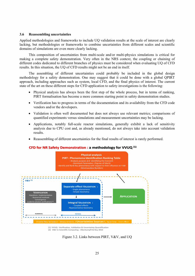
Uncertainty quantification (UQ) starts by clearly identifying the various sources of uncertainty. Figure 3.2 shows the two physical domains covered by V&V, i.e., the test conditions for SET and IET during the validation process, as well as the reality of interest which is presently a nuclear reactor named application domain. The validation domain is shown by the blue line; the yellow line shows the application domain.

UQ activities should concern both validation and application since all physical phenomena identified as important in the PIRT analysis must be present in the validation domain.

This section will not go into further detail on the UQ matter because the aim of this document is to establish a review of the existing methods and to initiate a state of the art on the UQ of CFD. However, before dealing with UQ of CFD in NRS demonstration, one should deal first with UQ of CFD results obtained during validation process. In the same way that PIRT is an iterative process, VVUQ also is.

As for V&V, users must run numerous sensitivity studies to give confidence to the simulation tool results. For the application step, users must run more sensitivity calculations to obtain sufficient data to reach statistically converged results. These sensitivity calculations, performed to check the quality of the base CFD calculation, must not be confused with the sensitivity analysis, which is performed in addition to UQ and makes identification of the main contributors to the uncertainty of FoM possible.

25

3.6 Reassembling uncertainties

Applied methodologies and frameworks to include UQ validation results at the scale of interest are clearly lacking, but methodologies or frameworks to combine uncertainties from different scales and scientific domains of simulations are even more clearly lacking.

This composition of uncertainties from multi-scale and/or multi-physics simulations is critical for making a complete safety demonstration. Very often in the NRS context, the coupling or chaining of different codes dedicated to different branches of physics must be considered when evaluating UQ of CFD results. In this situation, the UQ of CFD results might not be an end in itself.

The assembling of different uncertainties could probably be included in the global design methodology for a safety demonstration. One may suggest that it could be done with a global QPIRT approach, including approaches such as system, local CFD, and the final physics of interest. The current state of the art on these different steps for CFD application to safety investigations is the following:

• Physical analysis has always been the first step of the whole process, but in terms of ranking, PIRT formalisation has become a more common starting point in safety demonstration studies.

• Verification has to progress in terms of the documentation and its availability from the CFD code vendors and/or the developers.

• Validation is often well documented but does not always use relevant metrics; comparisons of quantified experiments versus simulations and measurement uncertainties may be lacking.

• Applications, notably full-scale reactor simulations, generally exhibit a lack of sensitivity analysis due to CPU cost and, as already mentioned, do not always take into account validation results.

• Reassembling of different uncertainties for the final results of interest is rarely performed.

Physical analysisPIRT : Phenomena Identification Ranking Table

- Analysis purpose and identifying the transient- Dominant Parameters (Figures of Merit)

- Identify and Rank Key phenomena with respect to their influence on FoM- Dimensionless Numbers

Separate effect VALIDATION :- Single phenomena- Simple Geometry

Integral VALIDATION :- Coupled effects

- Representative Geometry

APPLICATIONVERIFICATION

-Equations implementation- Numerical methods

Convergence(code & solution verification) (2)

Chaotic Flow behaviour – Measurements / Uncertainties Sources \ Input Data - User effect

V&V (1)

(1) VVUQ : Verification, Validation & Uncertainty Quantification(2) V&V in Scientific Computing - Oberkampft & Roy 2010

CFD for NR Safety Demonstration : a methodology for VVUQ (1)

NUMERICAL PHYSICAL

Figure 3.2. Links between PIRT, V&V, and UQ

26

4. SOURCES OF UNCERTAINTY IN LWR THERMAL-HYDRAULIC SIMULATIONS

4.1 The various sources of uncertainty in CFD applications to LWR

Theoretically, the sources of uncertainty in single-phase CFD are the same as for system codes, but

practically there are major differences in the relative weight of each source.

Here is a list of potential sources:

1. Initial and boundary conditions: When there is a flow entering the domain of simulation, the inlet

flow parameters often have a high uncertainty. For example, the mass flow rate at a pump outlet

can be hard to assess accurately because of uncertainties in the pump signature, unsteady flow

rate, or unknown pressure. More generally, initial and boundary conditions may result from a

system code calculation which gives only the 1D (area averaged) flow parameter whereas, CFD

requires 2D inlet profiles. Some simple assumptions may be used to give inlet profiles of

velocity, temperature, and turbulence intensity among others. When thermal coupling with

metallic structures plays a role, initial and boundary conditions are also required and might

necessitate rough approximations if detailed information is not available.

2. Uncertainties related to the parameters of physical models: Wall functions – if used – to express

momentum and energy wall transfers and parameters of turbulence models (e.g., C1, C2, Cm, Prk

and Pr ε of the k-ε model) are sources of uncertainty in the same way that all closure laws of

system codes are. Experts in turbulence may argue that these parameters were derived from basic

flow configurations and cannot be changed; however, models may be used beyond their domain

of applicability, and one may assign uncertainties related to this extrapolation.

3. Uncertainties related to non-modelled physical processes and uncertainties related to the form of

the models: Models may have inherent limitations. For example, an eddy viscosity model like k-ε

or k-ω cannot predict a non-isotropic turbulence nor an inverse-cascade of energy from small

turbulence scales to large ones.

4. Choice among different physical model options: When BPGs cannot give strong arguments to

recommend one best model option, one may consider all the possible model options compatible

with BPGs and consider the choice itself a source of uncertainty. This is called a “categorical

variable” in the extended propagation of uncertainty methods described in section 6.2.

5. Numerical uncertainties: Numerical uncertainties are related to the discretisation and to the

solving of the equations. They include time discretisation errors, spatial discretisation errors,

iteration errors, and round-off errors. BPGs give recommendations to control such errors.

However, a certain level of residual error may be accepted if one can estimate the resulting

uncertainty band on the prediction.

6. Choice among different numerical options: When BPGs cannot give strong arguments to

recommend one best numerical option, one may consider all the possible numerical options

compatible with BPGs and consider the choice of the option as a source of uncertainty. This is

also a “categorical variable” in the extended propagation of uncertainty method described in

section 6.

27

7. Simplification of the geometry: The geometrical details of a reactor may have some impact on the resulting flow. In code applications, some simplifications of the geometry may be adopted, and in all cases, details smaller than the mesh size are not described. This creates some non-controlled errors which should be considered in the UQ process.

8. Uncertainties due to scaling distortions: Situations may exist in which one can determine the uncertainty of input parameters in a given range of flow conditions characterised by geometry and the values of some non-dimensional numbers. In reactor applications, the geometry and values of some non-dimensional numbers can be out of the given range. In such a case, one should assign some uncertainty due to extrapolation from other geometry or other values of non-dimensional numbers.

9. Uncertainty due to previously measured data: Information coming from previous data may be used in a simulation, for example, the physical properties of fluid and solids. This information is known with some uncertainty, which will also affect the global uncertainty of code predictions.

10. Uncertainty arising from physical instabilities and/or chaotic behaviours: Under certain circumstances, nonlinear dynamic systems like Navier-Stokes equations can exhibit chaotic behaviours. Manneville (2010) reminds us that chaos results in unpredictability in the long term despite the fact that determinism guarantees predictability in the short term. Chaotic behaviours can be computed with small changes in the input data. The result has to be treated in a probabilistic framework. Since UQ generally appends in a probabilistic framework, there are ways to deal with such flows.

It's difficult to evaluate separately each source of uncertainty separately and at different scales (scaled mock-up and full reactor). ASME and EDF approaches (see sections 8 and 12) distinguish two types of uncertainties:

• A distance, bias, or scatter of simulation relative to reality when calculating IETs or CETs; and

• A scatter of the simulation results due to the multi-configuration of numerical parameters of the CFD simulation – a part of these parameters is selected during the validation, and it is not possible to set other parameters like initial conditions (ICs) and boundary conditions (BCs) or the mesh.

The uncertainties due to initial and boundary conditions may be propagated by the code.

Figure 4.1 shows a possible classification of the different sources of uncertainties for CFD. Note that the sources (2, 3, 8, and 9) identified above are not considered in this figure. The top square in the figure represents the global set of parameters for a given CFD simulation; the blue parts represent the parameters which are fixed by the V&V, e.g. the best turbulence model, boundary laws; the ones in green are related to ICs and BCs; and those orange show the relationship between the mesh and the numerical options of the code.

Using various sensitivity calculations and validation results, the bias and the scatter of CFD uncertainties must be determined. The final combination of uncertainties may need a probabilistic distribution of CFD results.

28

Figure 4.1. Identifying sources of uncertainty

4.2 Differences between system codes and single-phase CFD codes with respect to uncertainty

Apparently, large differences with respect to uncertainty exist between single phase CFD tools and system codes which solve mainly two-phase problems:

• Single phase CFD tools have very few physical models (e.g. turbulent viscosity, wall functions); whereas, system codes include hundreds of closure laws for wall transfers and interfacial transfers for each flow regime and for each flow geometry.

• Single phase CFD tools propose many options for the physical models (e.g. k-ε, k-ω, RSM, SST, RNG k-ε, LES, DES); whereas, system codes generally propose one set of standard validated closure laws. No extended validation exists for each physical option.

• Single phase CFD tools propose many options for the numerical scheme, while system codes generally propose one (i.e., CATHARE, ATHLET, TRACE, and SPACE codes) or two numerical schemes (i.e., RELAP-5 and TRAC codes).

• Single phase CFD tools do not propose a comprehensive validation matrix for each set of physical and numerical options; in contrast, system codes generally propose a very large, validated matrix – including both SETs and IETs – applied to a standard set of closure laws.

Single phase CFD tools may have CPU time difficulties running simulations with a converged meshing and time step. Therefore, many applications may have significant numerical errors. Such numerical errors may be equal or larger than the error due to physical modelling. System codes may also use non-converged meshing, but generally, the numerical error remains significantly smaller than the error due to physical modelling; thus, the former may be forgotten in the uncertainty analysis.

• Single phase CFD tools are able to simulate the effects of small-scale geometrical details of the flow; whereas, system codes are macroscopic tools that simplify the geometry of the flow, and

29

the effects of small-scale geometrical details (e.g. the geometry of spacer grids in a fuel assembly) are embedded in the closure laws, which were fitted on prototypical experiments.

In summary, one can list favourable and unfavourable aspects of UQ for single phase CFD compared to system codes.

The favourable aspects are:

• Single-phase flow issues depend on a relatively small number of non-dimensional numbers. In the list of governing non-dimensional numbers for mixing problems, the Reynolds and Prandtl or Schmidt numbers are always present; the Froude number is present in the case of density effects; a Nusselt number is present in case of heat transfer with walls; and in some transients, a Strouhal number – or other numbers – may be present; the available experiments may more or less easily cover the domain of similarity with respect to these numbers. In two-phase flows treated by system codes, many non-dimensional numbers exist, and no experiment can satisfy all of them;

• Single-phase CFD tools have very few physical models for which the uncertainty has to be determined;

• The simplifications of flow geometry for single phase CFD tools are less frequent and more limited than those in system codes; consequently, the portability of a physical model from a specific geometry to another is easier.

The unfavourable aspects are:

• When extrapolating from a scaled experiment simulation to a reactor simulation, the scalability of the numerical scheme, of the nodalisation, and of the physical models has to be investigated;

• If CFD is used with some degree of simplification of the geometry, the impact of such simplifications need to be taken into account in the uncertainty evaluation;

• Methodologies for uncertainty evaluation which require many calculations would be very difficult to apply to CFD due to high CPU cost;

• Since several options for the physical models (e.g. turbulence, wall laws) and several numerical schemes are possible, if BPGs do not give precise criteria to select the best option, this represents an additional source of uncertainty which must be taken into account;

• The absence of the results of a comprehensive validation matrix for single phase CFD does not help in the UQ process; quantifying the different sources of uncertainty listed in section 4.1 is more difficult than for system codes. This is the case for uncertainties related to the parameters of physical models. Indeed, the analytical experiments in which only a few of these models are influential are very specific (plane channel, isotropic homogeneous turbulence, etc.). More complex experiments exist, such as jets, plumes, and flows with obstacle, but they are difficult to use due to the overly high number of potentially influential parameters. The difficulty is still more important for the so-called categorical variables, such as the choice among different physical model options or among different numerical options: What level of probability can be given to each option? The hypothesis of equi-probability for each option is not necessarily justified.

30

5. CLASSIFICATION OF METHODS FOR UNCERTAINTY QUANTIFICATION

Code uncertainty methodologies for reactor thermal hydraulics were first developed for system codes which simulate many kinds of transients in an extensive range of single phase and two-phase conditions. They were based either on “propagation of the uncertainty of input parameters” (so called uncertainty propagation methods) or on “accuracy extrapolation” methods (see d’Auria and Galassi, 2010). Nowadays there are different software frameworks or platforms dedicated to uncertainty quantification. For instance we may mention URANIE1 the Uncertainty and Sensitivity platform developed by CEA. It aims at capitalising all methods and algorithms about uncertainty and sensitivity in the same framework and in particular it comprises most of the methodologies presented hereafter.

5.1 Methods based on propagation of uncertainties

The methods using propagation of code input uncertainties for thermal hydraulics with a link to NRS issues follows the pioneering idea of CSAU (NED Special Issue, 1990), later extended by GRS (Glaeser et al., 1994). This is the most-often-used class of methods. First, uncertain input parameters are listed and include initial and boundary conditions, material properties, and closure laws. Probability density functions (PDFs) are determined for each input parameter. Then the parameters are sampled according to their PDFs, and the reactor simulations are run with each set. In the GRS proposal, a Monte Carlo sampling is performed with all input parameters being varied simultaneously according to their PDF.

Perhaps because it relies on a limited number of assumptions, the Wilks theorem is often used to treat the results of uncertainty propagation and makes estimating the boundaries of the uncertainty range on any code response with a given degree of confidence possible. The number of code runs for an acceptable degree of confidence is around 100, although a higher number of code runs, typically 150 to 200, is advisable for better accuracy on the uncertainty ranges of the code responses.

More generally, propagation of uncertainties typically requires many calculations to reach convergence of statistical estimators, which may be difficult with CFD because of the amount of CPU time necessary. Fortunately, relatively simple statistical tools can give an estimate of the uncertainty resulting from datasets of limited size (bootstrap and Bayes formula, for example).

In the domain of uncertainty propagation methods, there are three trends:

• The Monte Carlo method uses a rather large number of simulations with all uncertain input parameters being sampled according to their PDFs. The resulting PDF of any code response is established, and the accuracy does not depend on the number of uncertain input parameters.

• Use of meta-models: in an attempt to reduce the number of code simulations, some methods consider only the most influential uncertain input parameters. These methods do a few calculations varying these uncertain input parameters in order to build a meta-model which replaces the code in order to determine the uncertainty on any code response with a low CPU cost. The Monte Carlo method is used with these meta-models performing several thousand runs. The use of meta-models such as polynomial chaos expansion and kriging became popular. These

1. http://sourceforge.net/projects/uranie/

31

meta-models provide a mapping between uncertain input parameters and model results built on a limited number of model evaluations. They necessarily rely on assumptions of regularity, or continuity, or shape of model responses and should be considered with caution when the assumptions are difficult to verify. Basically, in such a case, one might replace the non-convergence uncertainty of propagation methods that is rather easy to estimate with uncertainties due to approximations inherent in meta-models, which are more difficult to calculate.

• Unlike the first two, the deterministic sampling method does not attempt to propagate entire PDFs. Rather, it propagates statistical moments. The deterministic samples are chosen such that the known statistical moments are represented. If only the mean and the standard deviation, i.e., the first and second moments, are known, the uncertainty can be represented by two samples. They are chosen such that they have the given mean and the given standard deviation. Three samples are enough to represent the first four moments of a Gaussian distribution. Arbitrarily higher moments can be satisfied by adding more samples into the ensemble. This method does not suffer from the curse of dimensionality. Not only the variance of the marginal distributions but also covariance can also be built into the ensemble The method is very lean in number of samples, but the challenge lies in finding the right sampling points. Often, weighted samples need to be introduced.

Logically, uncertainty propagation methods require preliminary work to determine the uncertainties of closure laws. This determination can rely on expert judgement or, for a better demonstration, on statistical methods based on various validation calculations. Determining the uncertainty band or PDF for each closure may be easy when data sensitive to a single closure law are available. This is a SET in the full sense. In practice, data are often sensitive to multiple closure laws, and methods have been developed to determine uncertainty bands or PDFs for multiple closure laws based on several data comparisons with predictions (see de Crécy and Bazin, 2001–2004)

5.2 Accuracy extrapolation methods

For system codes, the methods identified as propagation of code output errors are based upon the extrapolation of accuracy. One can cite UMAE (d'Auria and Debrecin, 1995) and CIAU (d’Auria and Giannotti, 2000; see also Petruzzi and d’Auria, 2008). An extensive validation of system codes on both SETs and IETs allows the measurement of the accuracy of code predictions in a large variety of situations. In the case of UMAE and CIAU, a metric for accuracy quantification is defined using the Fourier Transform. The experimental database includes results from different scales, and once the accuracy of code results is assumed not to depend on the scale, this accuracy is extrapolated to reactor scale.

Methods based on extrapolation from validation experiments possibly require only one reactor transient simulation, but many preliminary validation calculations of integral test facilities are required.

5.3 The ASME V&V20

The ASME V&V20 standard for V&V in CFD and heat transfer states that “The concern of V&V is to assess the accuracy of a computational simulation” (2009). This view is clearly compatible with the principle of the methods based on extrapolation from validation experiments.

In current industrial CFD models (non-DNS), results come from solving a part of the Navier-Stokes equations and from modelling a part of these equations. Verification of correct solutions for these equations – called solution verification in Oberkampf and Roy (2010) – can be considered “tractable” even for complex flows. Once it is done, physical model uncertainty is a legitimate concern.

Different experiments tend to give significantly different model parameter values in calibration processes, indicating that the form and the generality of the model itself must be questioned. For example,

32

see different non-dimensional mixing lengths between 0.07 and 0.16 for different academic flow configurations in Rodi (1980).

5.4 Comparison of methods

Methods based on validation result extrapolation offer a poor mathematical basis but the comparison with reality, even in scaled experiments, may give an idea of the impact of model inadequacy on results at full scale. Even the impact of non-modelled phenomena is taken into account when we compare simulations to experiments, which is not so clear for uncertainty propagation. Obviously, extrapolation of results from scaled experiments to full scale is almost impossible to justify rigorously, regardless of the method used. If we were able to precisely estimate the physical model uncertainty, we would also be able to define a perfect model.

Another difference between the methods of propagation and extrapolation is the possibility of performing sensitivity analysis. Methods based on propagation allow such an analysis by using the results of the runs already performed for the uncertainty analysis. Sensitivity analysis is impossible with methods based on extrapolation because they do not consider individual contributors to the uncertainty of the response.

Benchmarking of system codes for the methods belonging to the two different classes was made as part of two international projects launched by OECD/CSNI. These are identified as UMS (OECD/CSNI, 1998) and BEMUSE (de Crécy et al., 2007). A significant lesson from these benchmarks is that the methods have now reached a reasonable degree of maturity, even if the quantification of uncertainty of the closure laws remains a challenge in propagation methods.

For CFD, no relevant benchmark has been established yet for comparing different approaches to test cases. Previously, we saw that uncertainty propagation and uncertainty based on validation result extrapolation are different in their nature and in their goals. In this context, setting up a relevant benchmark case to compare approaches belonging to these different classes seems essential.

5.5 The role of validation in SETs and IETs/CETs in the UQ process

All types of thermal-hydraulic codes, including system codes and CFD codes, use some kind of averaged equations. Local instantaneous equations such as continuity, Navier-Stokes, and energy equations are exact equations, but they cannot be solved directly due to excessive CPU cost. Averaging – time averaging, space averaging, or both – is necessary to reduce the time and/or space resolution to a degree that makes the calculation reasonably expensive. However, due to the averaging, some terms of the equations require some modelling to close the system of equations. Such relations are usually obtained by a theoretical derivation plus some fitting on appropriate experimental data. These models are approximations of the physical reality and cannot provide exact prediction of the averaged flow parameters. One can try to estimate the domain of uncertainty of these models or closure relations by using the same data basis and by finding the multiplier values which allow prediction of an upper and lower boundary of the data. This may result in a PDF for the multiplier.

This process may be executed using SETs in which one particular model or closure law is sensitive. In other SETs, measured parameters may be sensitive to a few models. In some cases, if various flow parameters are measured, one can identify the sensitivities in each influential model and determine the uncertainty of each model.

In IETs or CETs, all models of the code may have some influence on the parameters of interest. Estimating the relative weight of each model in an IET simulation is very difficult. Such IETs may be useful in the UQ process if they simulate the reactor transient of interest. The sensitive models and the relative weight of each sensitive model are similar in the IET and in the reactor transient. Such an IET or CET can thus be used to determine the error or uncertainty of code results applied to the reactor transient.

33

The uncertainty propagation methods mainly use SETs in the UQ process; whereas, accuracy extrapolation methods use more IETs. Both methods may require some scale extrapolation since both SETs and IETs are reduced-scale tests which cannot respect all non-dimensional numbers.

All types of thermal-hydraulic codes have intrinsic limitations related to phenomena which are not modelled. System codes use closure laws obtained for steady established flows in transient non-established flows, and the phenomena associated with non-establishment or transient effects are not modelled. This is a source of uncertainty. CFD codes use turbulence models which can never describe all geometrical effects in complex industrial geometries, meaning that all non-modelled effects comprise another source of uncertainty.

Simulation of IETs, which represent a reactor transient, with all the geometrical complexity takes these sources of uncertainty into account. However, if scale distortions between the IET and the reactor exist, it is never guaranteed that the relative weight of all sources of physical model uncertainties, including both closure model uncertainty and uncertainty relative to non-modelled physical processes, is similar which makes extrapolation difficult.

In the end, the comparison between simulations and experimental data is the only way to measure the error or uncertainty related to the physical model, but since often the only data available are reduced scale data, issues of scale extrapolation may be unavoidable in the UQ process.

34

6. AN UNCERTAINTY PROPAGATION METHOD EXTENDED TO CFD

6.1 Short description of the method

The method studied at Commissariat à l’énergie atomique (CEA) comes from the method used for system codes and is based on the propagation of input uncertainties. It is broadly used worldwide, for example, in the BEMUSE benchmark (de Crécy et al., 2007). For uncertainty analysis, this method consists of performing Monte Carlo code runs without using a meta-model. Consequently, numerous code runs of the CFD code are needed, typically 100 or even more. After completion of the code runs, order statistics are used to obtain statistical quantities for the responses, such as percentiles or tolerance intervals. By using the results of the performed code runs, a simple sensitivity analysis of the first order can be performed after the uncertainty analysis.

A very important advantage of this method is that there is no limit on the number of input parameters that can be considered. In addition, several types of input parameters can be considered. One can include initial and boundary conditions as well as parameters related to the physical models. Considering different options for physical modelling, for example, turbulence modelling, and for numerical schemes such as convection schemes is possible if BPG do not give clear recommendations on the best option. It is done by the use of so called “categorical variables”, more frequent in CFD codes than in system codes. Consequently, many sources of uncertainty quoted in section 4.1 are considered in this method.

One drawback of this method is that estimating the PDFs of these numerous input parameters is necessary. This estimation is challenging, and no method for that has been well investigated. Nevertheless, this drawback exists for all the methods based on the propagation of input uncertainties.

The main drawback specific to the CEA method is the high number of code runs needed, which can be a critical issue in CPU-consuming time reactor calculations. But one can hope that CPU time will decrease in the near future as technologies continue to develop. To avoid such CPU expense, methods are being investigated in which expensive runs of the most complex models are combined with relatively cheap runs using, for instance, degraded meshings, i.e. multi-level code models. A third drawback of the method is that all the code runs have to be successful for a proper application of the order statistics. This difficulty is not insurmountable but can require increasing the number of code runs, as shown in the application described in section 6.3.

6.2 Categorical variables and their treatment

Discretisation schemes are typical examples of categorical variables. For example, if the BPG recommendations are not clear enough, the user has different choices for the time scheme: explicit Euler, Runge-Kutta order 3, Cranck-Nicholson, etc. These alternatives correspond with different “levels” of the variable “time scheme”, which are neither numerical nor continuous. Consequently, this type of variable requires a specific treatment and can pose some difficulties.

6.2.1. Difficulty for uncertainty analysis

The first possible difficulty is with uncertainty analysis. Using statistics order requires that the PDF of the response is continuous. In other words, the different values of the response obtained by propagation must

35

be all different. The presence of categorical variables may introduce a certain degree of discontinuity in this PDF. More precisely, if all the variables were categorical, the PDF would be “perfectly discontinuous”, with a succession of peaks, each corresponding to the value of the response for a given combination of the levels of the categorical variables. With the mixing of categorical and real variables, the PDF of the response is smoother, but a certain level of discontinuity can still be present. This issue was investigated in the application described in section 6.3.

6.2.2. Difficulty for sensitivity analysis

The second difficulty concerns sensitivity analysis. Since categorical variables are not numerical, standard sensitivity measures such as standardised regression coefficients or correlation coefficients cannot be used. Two new measures are proposed.

The first type of sensitivity measure is based on regression techniques as used in the analysis of variance (ANOVA), where the presence of categorical variables is very frequent. Let us use H to denote the categorical variable, and let us assume that it has 𝑛𝑛 different levels. The linear regression is performed by replacing 𝐻𝐻 with (𝑛𝑛 − 1) real coded variables, denoted as 𝐻𝐻1 ,𝐻𝐻2 …𝐻𝐻𝑛𝑛−1, the values of which are 0, -1, or 1, according to Table 6.1:

Table 6.1: Values of the real coded variables 𝑯𝑯𝟏𝟏 ,𝑯𝑯𝟐𝟐, … ,𝑯𝑯𝒏𝒏−𝟏𝟏 , associated with a categorical variable 𝑯𝑯 with 𝒏𝒏 levels

Levels of the categorical variable 𝐻𝐻

Value of 𝐻𝐻1 Value of 𝐻𝐻2 … Value of 𝐻𝐻𝑘𝑘 Value of 𝐻𝐻𝑛𝑛−1

Level 1 1 0 0 0

Level 2 0 1 0 0

… Level 𝑘𝑘 0 0 1 0

Level 𝑛𝑛 -1 -1 -1 -1

Performing the linear regression using 𝐻𝐻1 ,𝐻𝐻2 …𝐻𝐻𝑛𝑛−1 makes it possible to obtain (𝑛𝑛 − 1) regression coefficients for these coded variables: ℎ1 for 𝐻𝐻1, ℎ2 for 𝐻𝐻2, …, and ℎ𝑛𝑛−1 for 𝐻𝐻𝑛𝑛−1. The last regression coefficient ℎ𝑛𝑛 is deduced from the other ones by: ℎ𝑛𝑛 = −ℎ1 − ℎ2 −⋯− ℎ𝑛𝑛−1.

Finally, if:

• there are nRV real variables, denoted as Xi, in addition to the H categorical variable;

• the regression coefficients of the Xi real variables are denoted as ai; and

• the response is denoted as Y,

36

Then the linear regression is written as follows if the 𝐻𝐻 categorical variable is at its level:

𝑌𝑌 = 𝑎𝑎0 + 𝑎𝑎𝑖𝑖

𝑛𝑛𝑛𝑛𝑛𝑛

𝑖𝑖=1

𝑋𝑋𝑖𝑖 + ℎ𝑘𝑘

And if the empirical frequency of the 𝑘𝑘𝑡𝑡ℎ level of 𝐻𝐻 is denoted as 𝑝𝑝𝑘𝑘 (close to 1 𝑛𝑛⁄ if the levels are equi-probable), the contribution of 𝐻𝐻 to the variance of the response is estimated using the following equation

𝑝𝑝𝑘𝑘

𝑛𝑛

𝑘𝑘=1

ℎ𝑘𝑘 −𝑝𝑝𝑘𝑘ℎ𝑘𝑘

𝑛𝑛

𝑘𝑘=1

2

The second type of sensitivity measure is based on correlation coefficients for the real variables and on conditional variance of the expectation value of 𝑌𝑌 knowing 𝐻𝐻 for the categorical variables. More precisely, for the real variables, if

• the correlation coefficient of the response Y and of the Xi real variable is denoted as ρ(Xi, Y), and

• the empirical variance of the response is denoted as var(Y),

then the contribution of 𝑋𝑋𝑖𝑖 to the variance of the response is classically estimated by

𝜌𝜌(𝑋𝑋𝑖𝑖 ,𝑌𝑌) × 𝑣𝑣𝑎𝑎𝑟𝑟(𝑌𝑌)

For the categorical variables, if 𝑒𝑒𝑘𝑘 is the mean value of 𝑌𝑌 when 𝐻𝐻 is at its level 𝑘𝑘, then the contribution of 𝐻𝐻 to the variance of the response is estimated using

𝑝𝑝𝑘𝑘

𝑛𝑛

𝑘𝑘=1

𝑒𝑒𝑘𝑘 −𝑝𝑝𝑘𝑘𝑒𝑒𝑘𝑘

𝑛𝑛

𝑘𝑘=1

2

i.e., the conditional variance of the expectation value of 𝑌𝑌 knowing 𝐻𝐻: 𝑣𝑣𝑎𝑎𝑟𝑟[𝐸𝐸(𝑌𝑌 𝐻𝐻⁄ )].

Both formulas for the contribution of 𝐻𝐻 to the variance of the response are very similar, but the ℎ𝑘𝑘 regression coefficients are different from the 𝑒𝑒𝑘𝑘 mean values of 𝑌𝑌 knowing 𝐻𝐻. Studies performed by CEA to date show that both measures give the same dominant input parameters. The two methods are an extension of the classical methods used for system codes; they are also rather crude and give only the dominant parameters, since they are first order approximations. Their advantage is that they do not require performing additional code runs with beyond those already performed for uncertainty analysis.

6.3 An application case: “The heating floor”

The method proposed by CEA was applied to a case with experimental data, the so-called “heating floor”. An uncertainty analysis is completed, and the uncertainty bands are compared to the experimental data. Sensitivity analysis using both sensitivity measures described above has not yet begun but is planned in the near future.

6.3.1. Description of the experiment and the reference calculation

The principle of the heating floor is summarised in figure 6.1. The heating floor consists of a square, cold cavity filled with air at 15°C and of a hot floor at 35°C. The cold air at 15°C enters the cavity at the top left-hand corner, and air exists the system in the bottom right-hand corner.

37

Figure 6.1: General scheme of the “heating floor”

The flow is stationary and presents convection and buoyancy effects. It is calculated by the CFD

code Trio_U developed by CEA. A 2D modelling and a k-ε modelling of the turbulence are used. Many

input variables are considered, as explained below, including several categorical variables, but for

convenience, the turbulence modelling is fixed.

The available experimental data are

• Profiles of temperatures and the vertical component of the velocities on the horizontal straight

lines defined as y = 0.1, 0.52, and 0.9 m.

• Profiles of the horizontal component of the velocities on the vertical straight lines defined as x =

0.1, 0.52 and 0.9 m.

A reference input data deck is defined with a choice for the different numerical options made by

expert judgement. In particular, a finite volume elements (FVE) meshing (see figure 6.2) consisting of

30×30 quadrangles divided into four triangles in the bulk of the cavity with two layers of meshes near the

walls. The fluid is supposed to be incompressible, and to satisfy the Boussinesq’s hypothesis.

38

Figure 6.2: The finite volume element meshing used for the reference calculation

6.3.2. The input-uncertain parameters

The first step in the CEA method is defining input uncertain parameters and quantifying their uncertainty.

Twenty-seven input parameters were considered and are briefly listed below:

• Parameters related to meshing:

o Type of meshing: finite volume differences (FVD), FVE, or industrial meshing with as many

equilateral triangles as possible (ICEM);

o Number of meshes in the bulk of the cavity;

o Number of layers of meshes close to the walls.

• Parameters related to the numerical schemes:

o Convection schemes;

o Weighting factor α for the ef_stab convection scheme (weighting between a centred second

order scheme and an upward first order scheme);

o Time schemes (implicit or explicit with implicit diffusion);

o Security factor on the time step in the case of an implicit time scheme.

Physical modelling parameters:

o Fluid density (only dependence on temperature as in Boussinesq’s hypothesis or the

additional dependence of the density on pressure);

o Wall laws, both for velocities and temperatures:

- Standard laws or thin boundary layer equations (TBLE) type laws;

- The Von Karman constant.

39

• Parameters of the k-ε model: Cε1, Cε2, Cε3, Cµ, Prk, Prε, PrT..

• Physical properties: thermal conductivity, viscosity, and thermal expansion – two possibilities for

the definition of temperature used to calculate them.

• Initial and boundary conditions: V, k, ε and T at the inlet and floor temperatures.

Nine of the variables are categorical, such as the choice of meshing and the type of convection

schemes, and 18 are real continuous variables. Some variables are dependent. For example, the allowed

convection schemes are neither the same used for FVD models nor for FVE and ICEM models. In the same

way, the security factor on the time step is different from one only for implicit schemes. This method takes

these dependencies are taken into account.

The input parameters are numerous and miscellaneous. The exception to this is that due to the fact

that considering multiple turbulence models would have increased the difficulty of the study significantly,

only the k--ε model is used for the turbulence model.

Arbitrary uncertainties are assigned to these parameters. The real variables are supposed to obey a

normal law, often with a standard deviation equal to 5% of the reference value except the temperatures and

the inlet velocity, because in these cases, experimental uncertainties were available. The different levels of

the categorical variables are supposed to be equi-probable.

6.3.3. The propagation step

The adopted experimental design is simple random sampling (SRS) as advised in BEMUSE for the system

codes (de Crécy et al., 2007). One hundred code runs were simultaneously launched. The duration of each

code run varied greatly ranging from 5 minutes to 1.5 days. The longer calculations were those with lower

security factors on the time step and the finest meshing, FVE and ICEM types.

Many code runs fail. In addition, some code runs converge perfectly but toward obviously wrong

solutions: for example, towards temperatures not included in [15; 35]°C or a central eddy rotating in the

wrong direction. For a correct application of the order statistics, these failed or spurious code runs cannot

be simply discarded and replaced by other ones with new combinations of the values of the input

parameters. Consequently, the reason of these failures or strange results is systematically investigated. A

number of coding “bugs” are found in Trio_U. But the main finding is that the reference input data deck is

not optimised, although it follows the Trio_U user’s guidelines written some years ago when the input data

deck was defined. The main inadequacies of the reference input data deck are as follows:

• No bounded value of the turbulent viscosity;

• Different time solvers for the three types of equations: momentum, turbulence and energy;

• k and ε at the inlet incorrectly calculated;

• No progressive meshing for FVD and FVE. An example of correct FVE meshing is shown in

figure 6.3:

40

Figure 6.3: Example of correct meshing for an FVE modelling

An important lesson learnt from this study is that the inadequacy of the input data deck is apparent only for a few combinations of values of the input parameters. Both reference calculations, with or without correction produce very close results.

All the code runs are performed again using the improved data deck: In the end, 300 to 400 code runs were carried out for this study.

6.3.4. Results of the propagation step

For each point of the different profiles (T, Vx, and Vy profiles as described above), the 2.5% and 97.5% percentiles were obtained by order statistics. The 100 response values were ranked from lowest to highest with the third value and the ninety-eighth value noted as the 2.5th percentile and the 97.5th percentile, respectively.

The potential difficulty mentioned above regarding the non-perfect continuity of the PDF of the responses due to the presence of categorical variables did not materialise. All the values of the responses were different, and ranking them by increasing order does not pose any problems.

The uncertainty bands derived from the 2.5th and 97.5th percentiles widely envelop the experimental data for the three temperature profiles, as shown in figure 6.4 for the temperature in the bottom part of the cavity.

41

Figure 6.4: Uncertainty band derived from the 2.5th and 97.5th percentiles for a temperature profile

The results are not as good for the velocity profiles, especially for Vx on the vertical straight line x = 0.1 m in the left part of the cavity and for Vy on the horizontal straight line y = 0.1 m in the bottom part of the cavity, as shown in figure 6.5.

42

Figure 6.5: Uncertainty band derived from 2.5th and 97.5

th percentiles for 2 velocity profiles (on the left the

horizontal component Vx; on the right vertical component Vy). The black ovals superimposed on the graphs

indicate the zones where the experimental data are not bounded by the uncertainty band.

6.3.5. Conclusion for the study

The method was successfully applied. Considering categorical variables did not raise particular problems,

in contrast to what was expected. The main difficulty in this study was the high number of failed or

spurious code runs. All of them had to be corrected, which required improving the initial reference input

data deck. A total of 300 to 400 code runs were needed for correct application of the method; whereas, the

initial number of code runs defined for the Design of Experiment was 100. Propagation is requiring both

for the code and the reference input data deck.

Despite the high number and the diversity of the input parameters, the uncertainty bands do not

envelop the experimental data perfectly. Several possible explanations for this exist. The first is that the

k-ε model used for turbulence is perhaps not most appropriate, and considering different turbulence models

might have been a better approach. A second possible explanation is that the 2D model of the cavity

prevented taking any 3D effects into account. Lastly, the ranges of variation of the input parameters were

arbitrarily determined, and perhaps they were not wide enough.

This study must be completed by conducting a sensitivity analysis using the new sensitivity

measures defined for the categorical variables. Knowing the relative contribution of each input parameter

to the global variance of the responses could allow researchers to make a more valid and accurate model

with better prediction capabilities.

6.4 Conclusions regarding the method

From a theoretical point of view, this method is simple, and its application to a case such as the “heating

floor” does not pose unsurmountable problems. Here is a summary of the advantages and drawbacks of the

method. The main advantage of the method is that it can consider numerous and varied input parameters.

Nevertheless, varying the numerical schemes as done in the application case, for example, is perhaps

questionable. Following the BPG would be more advisable, but they do not give always clear indications,

as for this application case. Estimating an error band coming from the discretisation error with a method

such as Richardson’s extrapolation and Grid Convergence Index (GCI) (ASME V&V, 2009; Roache)

might be preferable, but the discretisation error is not representative of the all the potential sources of

numerical uncertainty (e.g. the choice among different meshings).

43

An important issue not really tackled in the application case is the UQ of the input parameters. This difficulty exists for all methods based on the propagation of input uncertainties, for example methods based on meta-models. It is even more challenging for the CEA method because of the use of categorical variables. Up to now, no method exists to assign a probability to each possible response for a given categorical variable.

As previously stated, the main drawbacks of the method are the high number of code runs required and the fact that all of them must be successful.

6.5 Characteristics of the method

This method is based on the propagation of the uncertainty of input parameters. It does not use a meta-model. The method addresses uncertainty due to IC and BC and to physics as related to the parameters of physical models and the choice among different physical model options. By considering different numerical options, the method partly addresses uncertainty due to numerics. Using this method can make it possible to calibrate parameters such as those related to physical model, but this possibility has not still be applied.

However, several issues are not taken into consideration in this model. It does not address uncertainty related to non-modelled physical processes or uncertainty due to the simplification of the geometry. Neither the scaling issue nor discretisation, iteration, or rounding errors are considered.

This method requires numerous calculations as well as SET data. SET data are needed for the quantification of the uncertainties of input parameters such as those related to physical models. Up to now, this task has not been performed. A maximum of number of SETs has to be considered, but only 4–5 calculations of each SET are necessary. IET data are not used by the method. A minimum of 100 reactor calculations are needed. One hundred fifty to 200 code runs would be preferable.

The degree of maturity of the UQ method applied to CFD is low: The method has been established but should be improved and applied to simple test cases but not yet to a reactor calculation. Nevertheless, the degree of maturity of this method when applied to system codes is high, as shown in the BEMUSE benchmark.

44

7. UMAE METHOD APPLIED TO CFD

The University of Pisa is starting a study aimed at developing an uncertainty evaluation methodology for CFD application to NRS. Such a methodology is to be derived from, or inspired by, the Uncertainty Method based on Accuracy Extrapolation – Code with the capability of Internal Assessment of Uncertainty (UMAE-CIAU) methodology already available for system thermal-hydraulic NPP analysis. Basically, it would inherit the fundamental concept of obtaining uncertainty information through an extrapolation process from accuracy information stored in a “qualified” validation database. Hence, it would also involve methods and criteria for qualification, for example, of code, models, users, and experimental data, for the evaluation of accuracy, etc.

7.1 Brief description of UMAE

The UMAE (sketched in Figure 7.1) was proposed by the University of Pisa in the late 1980s and then further developed (see D’Auria et al., 1995; D’Auria et al., 1998; IAEA SRS N.23, 2002). Contrary to other methods, which address the evaluation of individual input uncertainties and their propagation through code application, the UMAE focuses on the “propagation of code output errors”. Information on accuracy is stored in a suitable validation database, and the final uncertainty is obtained by extrapolating the accuracy from relevant integral experiments to the NPP scale. The possibility of performing such extrapolation relies on the following basic principles and assumptions:

1. ‘The direct extrapolation of experimental data is not feasible; nevertheless, time trends of significant variables measured during counterpart tests in differently scaled facilities are quite similar: this fact must be exploited.

2. Phenomena and transient scenarios occurring in larger facilities, keeping nearly constant the other conditions (e.g. design criteria, quality of instrumentation, etc.), are closer to the plant conditions than those recorded from smaller facilities.

3. “Qualified” codes are indispensable tools to predict plant behaviour during nominal and off-nominal conditions.

4. The confidence in predicting a given phenomenon by the code must increase when increasing the number of analysed experiments related to that phenomenon.

5. The uncertainty in the prediction of plant behaviour cannot be smaller than the accuracy resulting from the comparison between measured and calculated trend; furthermore, accuracy (uncertainty) must be connected with the complexity of the facility (plant) and of the considered transient.

6. The effects of user and nodalisation must be included in the methodology.’

In short, application of the UMAE consists of an iterative process involving validation against experimental data that aims to achieve “qualified” nodalisations, i.e., such that the related prediction accuracy meets given acceptance thresholds. By applying similar criteria, a qualified nodalisation for the NPP analysis (referred to as an/the analytical simulation model) is obtained, provided that the similarity of

45

the phenomena observed in the test facilities and predicted by the plant calculations is demonstrated by proper analysis. In addition to nodalisation qualification, user qualification plays a crucial role.

Once a qualified NPP nodalisation is available, a single calculation is sufficient for a given transient, and the related uncertainty can then be obtained by accuracy extrapolation from a relevant database that has been collected. Uncertainty methods based on the propagation of input uncertainties require several sensitivity calculations and hence huge computational costs, while involving less effort in the qualification process and relying on engineering judgement to a larger extent.

The accuracy evaluation is another key step in the UMAE; it involves appropriate metrics for quantification and acceptance criteria. The accuracy evaluation “tool” adopted by the University of Pisa in the framework of UMAE-CIAU is the Fast Fourier Transform based methodology (FFTBM, see Ambrosini et al., 1990 and Prošek et al., 2002), which uses appropriate FoM to characterise the discrepancies between code calculation results and experimental data in the frequency domain. This “automated” approach somewhat reduces the influence of the engineering judgement upon the code result evaluation, although some degree of engineering judgement is still involved in setting acceptance thresholds, which to some extent are arbitrary.

46

Figure 7.1: UMAE flow diagram (also adopted within the process of development and application of

CIAU)

The key steps of the UMAE methodology, partly summarised above, are indicated in the flow diagram in Figure 7.1. In particular,

• The starting point is the selection of a “frozen” code version (a) resulting from a general qualification process (b), based on which it can be considered a tool of wide-spread international use.

• The red loop (FG) on the right side of Figure 7.1 represents the qualification process for the code, the nodalisation, and the code user in relation to the capability to predict an assigned transient.

o The ITF nodalisations (c) are developed by qualified users.

o The code validation is based on specific experimental data (d) that must include all key phenomena that are expected to occur during the transient of interest.

47

o The ITF calculation (e) is immediately followed by a qualitative analysis aimed at checking whether all relevant thermal-hydraulic features are captured, a necessary condition to proceed. Such a check involves a thorough characterisation of both the experimental data and the calculated results by subdividing the time frame into phenomenological windows (PhW) and then identifying key phenomena (KPh) and relevant thermal-hydraulic aspects (RTA) in each PhW, thus verifying the consistency between calculations and experiments.

o If the qualitative analysis step is successful, an accuracy quantification step (f) must be performed to characterise the code prediction by suitable figures of merit. A specific method is necessary. The one adopted by the University of Pisa is the FFTBM, which includes a set of acceptance criteria.

o Then, the fulfilment of the user and nodalisation qualification acceptance criteria is checked (g).

o The qualification process is complemented by the use of “generic” experimental data (h), which may not include all the key TH features of the transient of interest, and thus, they cannot take part in the accuracy extrapolation process but can still be used for independent validation.

• In case of success, the user can proceed via GI with the development of the NPP nodalisation (i), taking advantage of the experience gained in developing the ITF nodalisations.

• The NPP calculation (j) involves two steps:

a. a facility Kv-scaled calculation: boundary and initial conditions derived from ITF (via proper scaling) and

b. a realistic conditions calculation: nominal conditions used as boundary and initial conditions.

• The qualitative and quantitative analysis of the results of the two above calculations must show “similarity”, and the respective PhWs and RTAs must show consistency (k).

• If this check is successful, the nodalisation (or set of nodalisations) can be considered as “qualified” for the NPP analysis (m). It is referred to also as an analytical simulation model (ASM). Needless to say, the model must be run using “qualified code” by a “qualified user”.

• Provided that a number of conditions are met (see D’Auria et al., 1994 for details), and with the help of statistics, the accuracy in predicting target results can be extrapolated from the validation database, the data in which were gathered during the qualification process, to the NPP scale (l).

• The extrapolated accuracy is assumed to be the uncertainty affecting the ASM calculation results (n).

7.2 Short description of CIAU

CIAU was proposed in 1997 and has further developed and applied ever since (see IAEA SRS N. 23, 2002, and D’Auria and Giannotti, 2000) with the intent of overcoming the limitations of other existing uncertainty methodologies, particularly the large computational effort required for their application and the strong user effect upon the results of the uncertainty methodology application.

CIAU is a software tool that couples the RELAP5 code2 to the UMAE approach3 and automatically provides uncertainty evaluation associated with a specific NPP transient calculation in the form of uncertainty bands enveloping the code results for selected target variables.

2. The approach is extendable to any other system code.

48

The CIAU implementation and use, sketched in Figure 7.2, relies on the following concepts:

1. the UMAE qualification process (described above);

2. the “status approach” for characterising nuclear plant transient scenarios;

3. the separation and recombination of time-error and quantity-error; and

4. the error-filling and error-extraction processes.

The “status approach” involves the use of an arbitrary set of six relevant TH quantities representative of the selected scenario (such as upper plenum pressure, primary loop mass inventory, steam generator pressure, cladding temperature at 2/3 of core active height, core power, the largest of steam generator down comer collapsed levels) plus the time elapsed since the transient start to identify the status of the plant. In other words, the plant status corresponds to a point in a seven-dimension phase space. Furthermore, if all the dimensions of such phase space are discretised, the status is then uniquely identified by a hypercube. The evolution of the plant during the transient is represented by a succession of hypercubes.

A key assumption is that the code prediction uncertainty, for selected output variables, is the same for all plant statuses falling within each discrete plant state. Therefore, by means of an uncertainty evaluation method – particularly by the accuracy evaluation of experimental test simulations performed in the framework of the UMAE qualification process –, a seven-dimension matrix of “quantity uncertainties” and a vector of “time uncertainties” can be filled up (error-filling process) so as to constitute a sort of uncertainty database that can be “looked up”.

With the availability of the uncertainty database, the application of the CIAU requires negligible computing effort and engineering judgement. Instead, those efforts were invested in the filling process.

Within the CIAU framework, the UMAE is considered more as a tool for qualifying the TH calculations needed to populate the hypercubes than as a method for uncertainty evaluation.

Although the influence of the user is inherently minimised by the application of the UMAE, the residual user effect is taken into account as a contribution to the overall uncertainty.

3. In principle, a different UQ method could be implemented in the CIAU as well.

49

Figure 7.2: Simplified flow diagram of CIAU

Here is the key to Figure 7.2:

• Part related to CIAU development:

a. Availability of “qualified” experimental data is implied.

b. Availability of “qualified” system code calculation results is implied (qualified code + computer + nodalisation + user).

c. Reference is made to selected postulated transients, characterised by using the “status approach”.

d. Qualitative, quantitative, and time accuracy are obtained through proper analysis and comparison of experimental data and code results..

e. A number of variables are selected as targets for the uncertainty evaluation.

f. Provided that acceptance criteria are met according to UMAE through step (d), a quantitative accuracy matrix is completed.

g. A time accuracy vector is also completed.

h. The scenario independence check must verify whether or not the calculated uncertainties in each hypercube are affected by the transient type.

i. If the scenario independence check is not satisfied, then the ranges of variation of the driving quantities must be changed or the transient type must be identified inside each hypercube.

m. If the scenario independence check is satisfied, uncertainty values can be directly assigned to each plant status. Thus, a quantity uncertainty matrix (QUM) is generated.

n. A time uncertainty vector (TUV) is also generated.

• Part related to CIAU application:

o. Once the QUM and TUV are available, the CIAU code application is straightforward.

50

p. An ASM calculation is run for a selected transient scenario. The six selected driving quantities (see above) are used to identify the succession of hypercubes that corresponds to the calculated transient.

q. If a failure occurs or if the uncertainty quantification is not required, the process stops here.

r. In order to characterise the transient status, time intervals are identified as well.

s. By looking up the obtained hypercubes and time intervals in the database, quantity uncertainty is obtained.

t. Time uncertainty is also found by accessing the database.

u. By means of the proper computing tool embedded in CIAU, the above quantity and time uncertainties are combined to obtain continuous lower and upper uncertainty bands.

7.3 Towards a UMAE-CIAU-like approach to CFD UQ

The basic goals/objectives are to develop the following

1. a qualification methodology similar to UMAE as applicable to CFD based on systematic and consistent exploitation of experimental data and on proper scaling and similarity analysis, which allows computational models with proven and quantified prediction capabilities to be obtained and to gather accuracy information for uncertainty extrapolation purposes;

2. a database of accuracy and uncertainty information obtained from the validation against differently scaled test facilities and possibly real plant data, using the application of the above method, and

3. an automatic tool similar to CIAU which allows the “internal assessment of the uncertainty” while minimising the computational effort and the impacts of user effect and engineering judgement.

The first major task is to define unambiguous qualification criteria for a code, for a code user, for a computational model, and for calculation results. Many qualification-related aspects have already been addressed by the BPGs (Mahaffy et al., 2007), which provide some useful guidance regarding model selection, mesh generation, code and calculation verification, and error reduction and quantification techniques. However, the BPGs do not include detailed guidance on specific applications or scaling and similarity analysis, nor on criteria for accuracy evaluation. Therefore, although the BPGs are a key reference, they need to be extended and complemented by additional guidelines.

Within a UMAE-like iterative qualification process, the accuracy evaluation plays a crucial role: This is the point at which decisions are made as to whether a given model is providing “acceptable” results, both qualitatively and quantitatively. The following needs can be identified:

• A rigorous approach to the qualitative analysis of code calculation results, aimed at assessing the code/model/user capabilities to exhibit all the thermal fluid dynamic aspects that are deemed relevant for the specific problem addressed in their predictions. For example, in a problem involving perturbation of time and space distribution of the coolant properties inside the reactor pressure vessel (RPV), first checking if a calculation has been able to reproduce the “morphology” of such a perturbation (which is very sensitive to the type of transient, to the presence of buoyancy, to possible asymmetries in the loop flows, etc.) may be important. Proceeding with the quantitative analysis if the qualitative predictions are unsatisfactory could be useless. Obviously, this step necessarily requires engineering judgement.

• Suitable metrics for the quantification of the accuracy require that one be able to make statements as to “how far” (in quantitative terms) a given calculation is from the simulated experiment. This

51

step may be more difficult for CFD than for TH system code analysis as multi-dimensional and multi-variable quantities are inherently involved. An attempt was made at the University of Pisa (see Moretti and D’Auria, 2014) to address this issue and propose a method to quantitatively compare CFD code results and experimental data for in-vessel mixing flow problems.

• Accuracy acceptance criteria, consistent with the adopted accuracy quantification metrics, and possibly connected with NPP licensing requirements are needed.

Another crucial aspect is the scaling and similarity analysis of both experiments and calculations. The following needs have been identified:

• The scaled test facilities and the experiments selected for the qualification process must be proved to be representative of the relevant phenomena and processes occurring at the NPP scale.

• Differently scaled test facilities must be referenced in order to perform the necessary assessments regarding model performance and the scale effect upon the code.

• The accuracy of code predictions must be proved not to diverge at increasing scales; otherwise, the assumption that the accuracy can be extrapolated fails and a UMAE-like approach cannot be applied.

Other important aspects to be addressed, in view of a translation of the UMAE-CIAU framework for CFD UQ purposes, are

• Identification and classification of relevant phenomena, processes, situations of interest, scenarios, etc.

• Identification of the specific needs and peculiarities of CFD compared to TH system codes, e.g. mesh related issues, accuracy quantification techniques, scaling.

• Making available a “generically qualified code” of criteria involving V&V and Quality Assurance (QA).

• Availability of suitable experimental data based on criteria to specify the level of quality in data that is required for the qualification purposes, e.g. CFD-grade data supplied with experimental uncertainty information, proper characterisation of BICs, and so on)

• Account of the experimental uncertainty should be included in the uncertainty evaluation.

• To address the user-effect issue, a sort of user self-qualification process should be implicit in the methodology as it is in UMAE-CIAU; possibly, criteria should be specified in terms of user qualification.

• Techniques to extrapolate the uncertainty from the accuracy, possibly involving statistical tools, need to be developed.

Among the fundamental concepts of the UMAE-CIAU methodology are the “status approach” and the multi-dimensional, coarsely-discretised phase space defined by a set of selected driving quantities. If – and to what extent – such concepts can be extended to the CFD application domain needs to be investigated.

The development work should create not only a methodology but also software tools to support practical implementation of the methodology. At a minimum, the software framework should include and/or support the following functions:

• Storage, management, and analysis of the experimental database;

• Automated accuracy quantification (similar, for example, to FFTBM tools);

52

• Storage, management, and analysis of the code assessment database (e.g. code results, calculation-to-experiment comparisons, error/accuracy/uncertainty information); and

• An automated accuracy-to-uncertainty extrapolation tool.

In its initial stage, the development of the methodology should focus on a limited spectrum of NPP applications for which a reasonably wide validation basis is available. The most appropriate choice seems to be the single-phase in-vessel coolant flow: boron dilution/mixing, asymmetric temperature distribution, PTS, accounting also for buoyancy, conjugate heat transfer, etc. A number of test facilities that have provided noticeable amounts of “mixing data”, albeit with a rather limited range of scales, and have fed intensive code validation activities within the international community exist. Defining separate approaches for steady-state and transient problems may prove necessary.

Even assuming that a complete and exhaustive methodology is developed and becomes available soon, along with the necessary software support tools, its implementation would certainly require intense engineering and computational effort before a relevant accuracy/uncertainty database can be established. Creation of the database will probably be the main challenge, however well motivated by the attractive idea of a fast and automated procedure for the CFD uncertainty extrapolation to NPP the nuclear engineering community is.

7.4 Characteristics of the method

The method is based on the extrapolation of uncertainty from accuracy. It does not use any meta-code. Neither does it individually address the uncertainty due to physics, numerics, nor geometric simplifications nor due to any other individual source of uncertainty. All contributions to the uncertainty of the calculation results are accounted for collectively, including the user effect. No specific method to address the scaling issue has been developed yet; however, the methodology necessarily requires that the scaling issue be addressed. No code calibration on data is envisaged.

As a part of the UMAE-like qualification process and particularly as a means to collect accuracy information from the validation and store it into an accuracy database, both SET and IET calculations are required. Under certain conditions, uncertainty can be extrapolated from the SET and IET calculations; therefore, the more SET and IET calculations that can be incorporated, the better, provided that qualified experimental data sets are available. As far as the uncertainty evaluation step is concerned, once a qualified model has been setup and an accuracy database is available, a single reactor calculation is sufficient: No further validation calculations, sensitivity analyses, etc., are necessary.

Currently, the level of maturity of this UQ method is very low: The basic ideas and the roadmap for the development have been established, and experience from the development of UMAE and CIAU can be exploited; however, most of the developmental work has yet to be performed. Moreover, a successful implementation of the method will certainly require an upgrade of the existing experimental database in order to make qualified data available for the UMAE-like qualification process and to support the scaling analysis.

53

54

8. SUMMARY OF THE ASME METHOD

The American Society of Mechanical Engineers (ASME) has worked on a standard for V&V and UQ for CFD and heat transfer applications (ASME V&V 20-2009).

The ASME standard conforms to Nuclear Regulatory Commission (NRC) and other regulatory practices, procedures, and methods for the licensing of nuclear power plants as embodied in the United States Code of Federal Regulations and other pertinent documents such as the Regulatory Guide 1.203 “Transient and Accident Analysis Methods” and NUREG-0800 “NRC Standard Review Plan” .

The standard V&V 20-2009 affirms that “The ultimate goal of V&V is to determine the degree to which a model is an accurate representation of the real world”. This standard is strongly based on the use of experimental data for V&V and consequently for UQ. With this approach, ASME makes a strong link between V&V and UQ.

The global VVUQ process is given below in Figure 8.1. This diagram only deals with uncertainties at the experimental scale. An additional step can be used to upscale from experimental to reactor scale.

𝑢𝑢𝑣𝑣𝑣𝑣𝑣𝑣 = 𝑢𝑢𝑛𝑛𝑛𝑛𝑛𝑛2 + 𝑢𝑢𝑖𝑖𝑛𝑛𝑖𝑖𝑛𝑛𝑡𝑡2 + 𝑢𝑢𝐷𝐷2

55

Figure 8.1: Errors and uncertainties in the validation process (reprinted with permission from ASME V&V 20-2009,)

According to the standard VV-20-2009, the comparison error E in any validation process is defined as the difference between the simulation result, denoted by S, and the experimental value D. This difference is expressed by means of the equation:

𝐸𝐸 = 𝑆𝑆 − 𝐷𝐷

If we denote T as the true value, then the comparison error can be split into the following:

𝐸𝐸 = 𝑆𝑆 − 𝑇𝑇 − (𝐷𝐷 − 𝑇𝑇)

Then, one defines the experimental data error 𝛿𝛿𝐷𝐷 and the simulation error 𝛿𝛿𝑆𝑆, as follows:

𝛿𝛿𝐷𝐷 = 𝐷𝐷 − 𝑇𝑇

𝛿𝛿𝑆𝑆 = 𝑆𝑆 − 𝑇𝑇

Because the simulation error 𝛿𝛿𝑆𝑆 has three components, the first one is the error due to the modelling process 𝛿𝛿𝑛𝑛𝑚𝑚𝑚𝑚𝑚𝑚𝑣𝑣; the second is the numerical error 𝛿𝛿𝑛𝑛𝑛𝑛𝑛𝑛 produced by the numerical algorithm and the discrete mesh used to solve the modelling equations; and the third is input errors (IC BC, properties,..;) 𝛿𝛿𝑖𝑖𝑛𝑛𝑖𝑖𝑛𝑛𝑡𝑡 . Therefore, the expression for the comparison error E can be written as

𝐸𝐸 = 𝛿𝛿𝑛𝑛𝑚𝑚𝑚𝑚𝑚𝑚𝑣𝑣 + ( 𝛿𝛿𝑖𝑖𝑛𝑛𝑖𝑖𝑛𝑛𝑡𝑡 + 𝛿𝛿𝑛𝑛𝑛𝑛𝑛𝑛 − 𝛿𝛿𝐷𝐷)

Thus, E is the overall result of all the errors coming from the experimental data and the simulation. Three assumptions are made: (1) D is based on an average of individual measurements, (2) the error 𝛿𝛿𝐷𝐷 is computed using the ordinary methods of the experimental fluid dynamics, (3) the same assumption is valid for the experimental uncertainty 𝑢𝑢𝐷𝐷. Therefore, the uncertainty in the comparison error is given by the expression:

𝑢𝑢𝐸𝐸 = 𝑢𝑢𝑛𝑛𝑚𝑚𝑚𝑚𝑚𝑚𝑣𝑣2 + 𝑢𝑢𝑖𝑖𝑛𝑛𝑖𝑖𝑛𝑛𝑡𝑡2 + 𝑢𝑢𝑛𝑛𝑛𝑛𝑛𝑛2 + 𝑢𝑢𝐷𝐷2

The components of the simulation uncertainty that can be estimated are the numerical simulation uncertainty 𝑢𝑢𝑛𝑛𝑛𝑛𝑛𝑛, the input uncertainty 𝑢𝑢𝑖𝑖𝑛𝑛𝑖𝑖𝑛𝑛𝑡𝑡, and the experimental uncertainty 𝑢𝑢𝐷𝐷 . However, no known method to estimate the modelling uncertainty 𝑢𝑢𝑛𝑛𝑚𝑚𝑚𝑚𝑚𝑚𝑣𝑣 exists. To solve this problem, the unknown error 𝛿𝛿𝑛𝑛𝑚𝑚𝑚𝑚𝑚𝑚𝑣𝑣 produced by the modelling is isolated:

𝛿𝛿𝑛𝑛𝑚𝑚𝑚𝑚𝑚𝑚𝑣𝑣 = 𝐸𝐸 − ( 𝛿𝛿𝑖𝑖𝑛𝑛𝑖𝑖𝑛𝑛𝑡𝑡 + 𝛿𝛿𝑛𝑛𝑛𝑛𝑛𝑛 − 𝛿𝛿𝐷𝐷)

E, its sign, and its magnitude are known. Next, the validation uncertainty VU is defined as an estimation of the standard deviation of the combination of errors 𝛿𝛿𝑖𝑖𝑛𝑛𝑖𝑖𝑛𝑛𝑡𝑡 + 𝛿𝛿𝑛𝑛𝑛𝑛𝑛𝑛 − 𝛿𝛿𝐷𝐷. If these errors are really independent, the combined validation uncertainty is given by the expression:

𝑢𝑢𝑣𝑣𝑣𝑣𝑣𝑣 = 𝑢𝑢𝑖𝑖𝑛𝑛𝑖𝑖𝑛𝑛𝑡𝑡2 + 𝑢𝑢𝑛𝑛𝑛𝑛𝑛𝑛2 + 𝑢𝑢𝐷𝐷2

𝑢𝑢𝑛𝑛𝑚𝑚𝑚𝑚𝑚𝑚𝑣𝑣2 may be given by

𝑢𝑢𝐸𝐸2 = 𝑢𝑢𝑛𝑛𝑚𝑚𝑚𝑚𝑚𝑚𝑣𝑣2 + 𝑢𝑢𝑣𝑣𝑣𝑣𝑣𝑣2

The ASME standard gives solutions to evaluate every term of the validation error (E) and the validation uncertainty (uval). Propagation methods are primarily used to evaluate uncertainties of input parameters. Uncertainties of numerical solutions are given by the code verification step. The standard indicates how to use E and uval. These quantities give an accuracy of the model used. If E >> uval, the

56

model used induced more error than the uncertainty indicating the model can be improved in order to reduce the uncertainty in the results. In contrast, if E < uval, the major uncertainty is in the uncertainty validation, which means that the model accuracy cannot be improved if this uncertainty cannot be reduced. The standard indicates that in individual cases, this is not proof that the model is good or bad but merely gives a warning about potential issues. The engineer has to evaluate the uncertainty according to his purpose.

ASME approach treats experimental and numerical results of interest as scalars with uncertainty. Oberkampf and Roy (2010) have described a similar methodology but for any kind of code results. Quantities of interest are considered “p-box”, which means probability distributions considering epistemic uncertainties. Same addition of terms is made to evaluate code uncertainties, but specific mathematics for probability distribution are used. This could/might be more suitable for complex quantity of interests (for example, CFD transient results).

Scaling uncertainty is not discussed in the ASME standard, but a chapter in Oberkampf and Roy (2010) is dedicated to “prediction”. The main issue in error and uncertainty evaluation for scaling is that the “real” quantity of interest at reactor scale is unknown. One option is to use only code results to evaluate scaling uncertainties. The main assumption is then that the variation of code results between the experimental facility and reactor scale is equivalent to the “real” variation between both scales. Another option is to use multiple experiments varying scaling factors like the Reynolds number or Froude number. If available, a set of experiments can lead to defining a validation domain that contains the application domain or provides some information for extrapolation outside of the validation domain.

The ASME standard methodology for uncertainty analysis underlines the role of V&V in the process of evaluating the confidence in CFD results. Uncertainties have to be evaluated step by step using clearly defined numerical aspects of the model such as time and space discretisation (time step and mesh convergence) or physical models (turbulence models, physical assumptions) with associated evaluation of error.

8.1 Characteristics of the method

The ASME method is not a UQ method for reactor application as it describes the UQ of a validation calculation. It does not address upscaling from the scaled experiment to the reactor. However, it may be used as a step in a general UQ method associated with an extrapolation method. Below is a summary of its characteristics.

It addresses uncertainty due to IC and BC, to physics as a whole, and to numeric.

It does not use a meta-code.

SET are not used in the method.

IET data are used in the method.

The ASME method also has some limitations. It does not address scaling issues. It does not specifically address uncertainty due to simplification of the geometry, but this may be included in the uncertainty due to numerics. There is no code calibration for the data. The maturity of the ASME method is low in the context of NRS applications.

57

9. UNCERTAINTY QUANTIFICATION USING THE DETERMINISTIC SAMPLING METHOD

The goal of this method is to predict how the results from a simulation are affected by one or more uncertain input parameters. These uncertain parameters might be any physical model constant, the value of a fluid or solid property, boundary condition values, or geometric parameters. The term deterministic is used as opposed to random. Random sampling is used in the Monte Carlo simulation, where the parameter values are randomly generated to satisfy a specified PDF. In the deterministic sampling (DS) method, the parameter values are instead calculated (Julier and Uhlmann, 2004; Hessling, 2013). Unlike the ensemble in the Monte Carlo method, which tries to represent a continuous PDF, the DS method represents the PDF with an ensemble that has the same statistical moments but contains much fewer samples. Each sample requires one simulation. In the DS method, the required number of simulations can be reduced substantially: by a factor of at least four orders of magnitude. This is key to be able to afford UQ in CFD and in all other simulations with long execution times.

9.1 Statistical moments

In DS, one tries to satisfy the statistical moments of a PDF. The first statistical moment is the mean, the second moment is the variance, the third is the skewness, and the fourth is the kurtosis or flatness. For a parameter, q, with an ensemble containing N samples, these can be written

qqN

mean N

i i == ∑ =1

1

21

)(1var qqN

N

i i −= ∑ =

331

/)(1 σqqN

skewness N

i i −= ∑ =

441

/)(1 σqqN

flatness N

i i −= ∑ =

where the standard deviation is

var=σ .

The nth statistical moment can be written

nnN

i ith qq

Nmomentn σ/)(1

1−= ∑ =

.

Arbitrarily higher moments can be represented with DS by adding new samples to the ensemble. To represent the mean and the variance of a parameter, q, a minimum of two samples is required.

58

9.2 A one-parameter example

A small example is set up to illustrate how the two methods compare. In this case, the Monte Carlo method is assumed to give the correct result but is computationally expensive.

Let f(q) be a nonlinear function where q is a parameter: 4)( qqfh ==

Assuming the parameter q has a normal PDF with a mean value 𝑞𝑞 =2 and a standard deviation σq=0.4. A Monte Carlo simulation is performed and will be taken as the norm for this case and is compared to a DS simulation in which initially only two samples are used in the ensemble. In the original unscented transform (Angrisani et al., 2006) for one parameter, two samples in an ensemble can be chosen as

q

q

qqqq

σ

σ

−=

+=

2

1

The location of q1 and q2 are called sigma points. This ensemble has the same mean, and standard deviation as a continuous normal distribution. Propagating these two samples through the function will give us

42

41

)4.02(

)4.02(

−=

+=

hh

The output average and standard deviation from the ensemble, containing two samples, are;

312.138656.19

2

2

==

DSh

DShσ

Figures 9.1 and 9.2 illustrate how many samples the Monte Carlo method requires to reach their designated values for the first two statistical moments of the input parameter q.

Figure 9.1. Evolution of mean value for input parameter, q, with the number of Monte Carlo (MC)

samples

59

Figure 9.2. Evolution of standard deviation for input parameter, q, with the number of Monte Carlo(MC)

samples

Figure 9.3. Evolution of mean value for the output value, h, with the number of Monte Carlo (MC) samples

60

Figure 9.4. Evolution of standard deviation for the output value, h, with the number of Monte Carlo

(MC)samples.

The asymptotic values for the mean and the standard deviation from the Monte Carlo simulation can

be found in Figures 9.3 and 9.4.

43.1587.19

==

MCh

MChσ

q

q

qq

qqqq

σ

σ

3

3

3

2

1

−=

=

+=

Each sample has a weight associated with it (see Julier & Uhlmann, 2004; Angrisani et al. 2006), and these are the weights chosen for this example:

61

64

61

3

2

1

=

=

=

W

W

W

61

Now the four moments are satisfied:

4433

422

411

333

322

311

233

222

211

2332211

/))()()((3

)()()(0

)()()(

q

q

qqWqqWqqWqqWqqWqqW

qqWqqWqqWqWqWqWq

σ

σ

−+−+−=

−+−+−=

−+−+−=

++=

By using these three samples we get

37.15)()()(

91.192

332

222

11

332211

=−+−+−=

=++=

hhWhhWhhW

hWhWhWh

hσ

,

which agree well with the results obtained from thousands of samples in the Monte Carlo method. This is achieved with just three deterministic samples. To be able to use the Monte Carlo method, a continuous PDF was assumed. From it, all the higher moments can be calculated. However, more often than not, not enough information is available to make this assumption. Often, only the variance, or covariance, and the mean value of a parameter are known. Applying a continuous PDF in such a case is pure guesswork, and the DS method will suffice. In addition, by including more samples in our ensemble, arbitrarily high moments can be represented, if they are known.

For the sake of comparison, a linear approximation (LIN) (see ISO GUM, 1995) of the function h = q4 gives the mean and standard deviation:

8.12*4*

.16

3

4

==∂∂

=

==

qqh

LIN

qqf

qh

LINσσσ

Clearly the LIN-method gives a poor estimate for both the average and the standard deviation.

9.3 Inverse uncertainty quantification

Statistical moments in the DS method can be adjusted in two ways. One is to adjust the location of the sigma points; the other is to modify their weights. This can be exploited in inverse UQ and when calibrating models. The problem with inverse UQ is the difficulty in finding an inverse function which can be used to propagate a result back to its original parameters, the so called “inverse problem”. One common technique is to replace the original function with a simpler surrogate model or a response surface. However, there is no need for this in DS. While the parameters propagate non-linearly though the function, the weights do not. They propagate linearly in both the forward and the inverse problems. We can thus adjust the weights of our ensemble in the result so it will fit the statistical moments of results we are using as a reference. This reference must be trusted experiments or otherwise known data. If one accepts this view, there is symmetry between the forward problem and the backward problem. We can adjust the weights of the input parameters so their statistical moments fit with the information we have about them. We can do a similar process for the reverse problem. We can modify the weights to tune our ensemble from the calculations to fit with the statistics we have from the reference results. When applying these new

62

weights to the input parameters, we get a new estimate of how uncertain our input parameters are. We can do this due to the fact that the weights propagate linearly. This gives us the uncertainty of the input, and no expert judgement is necessary. This uncertainty includes model inadequacies that are systematic and epistemic.

9.4 Summary

The method of DS has been exemplified in a simple case, which demonstrates its efficiency compared to the Monte Carlo method. For a nonlinear function, the DS method is more accurate than a linear method of propagating the mean and the variance. Its accuracy increases with the number of statistical moments satisfied by the ensemble. The DS method is only shown here in a one-parameter case. For a problem including many uncertain parameters, the reader is referred to Hessling (2013).

9.5 Characteristics of the DS method

The DS method propagates known statistical moments, not continuous distribution functions that are seldom known anyway.

DS does not require meta-code, but software that calculates the location of the sigma points and their weights is helpful.

It can include uncertainty in IC and BC as long as they are expressed as a function of parameters. Uncertainty due to the shape of a profile in BC or IC is not estimated at present, unless given as a function of the parameters.

The method has been used to estimate the uncertainty of the results due to uncertainty in the physical modelling constants. (See Nureth-16, 2015: “Use of Deterministic Sampling for Uncertainty Quantification in CFD”.)

• Non-modelled physical processes (e.g. a k-ε model cannot predict a non-isotropic turbulence) can be treated with the DS method through an inverse uncertainty quantification step. By adjusting the sample weights in the simulated results, these can be made to fit the results from “true” data through regression analysis. The new weights can be applied to the uncertain input parameters, which now do not include any expert judgement. In this fashion, an estimate of the systematic/epistemic uncertainty can be made for the physical model and related to the parameters of physical models.

• related to non-modelled physical processes (e.g., a k-ε model cannot predict a non-isotropic turbulence),

• Choice among different physical model options.

If DS is used with a calibration step, it will include the uncertainty due to the numeric as well as the model uncertainties. For the problem below, it is not included. A Richardson extrapolation could instead give an estimate to the uncertainty.

• Related to discretisation errors, iteration errors and round-off errors.

• Choice among different numerical options:

The DS method is not addressing uncertainty due to simplification of the geometry.

The DS method can address scaling issues (e.g. scalability of code physics and numerics, scale distortion of validation data) by treating the Reynolds number, the Froude’s number, and so on as uncertain parameters.

DS has never been tested for SETs or IETs for reactor application. However, the method appears to be an example of having multiple uncertain parameters and/or multiple models. DS is probably the leanest

63

method when it comes to number of samples required. In addition, the number of samples does not grow quickly with the number of uncertain input parameters. When dealing with alternative physical models, DS assigns each model a sample, makes the calculation, and assesses the level of uncertainty in the result. In a calibration step, a weight could be calculated for each sample to produce the best result. In this way, DS can achieve a good mix of models. If uncertain parameters are present in the physical models, each model is given an ensemble of several samples that best represent its input parameters. If we have multiple models in addition to uncertain parameters in the physical models, DS makes ensemble of ensembles. DS treats parameters and physical models in a similar fashion.

The DS method can be favourably used for calibration purposes. Calibration can be performed by adjusting the sample weights to fit the expected value and covariance of the known and trusted results.

The minimum number of samples and/or calculations required for the DS method is the number of uncertain parameters (n) plus one, n + 1. In this case, the mean and the variance can be propagated. For higher statistical moments, additional samples are needed.

The degree of maturity of DS is low.

64

65

10. POLYNOMIAL CHAOS EXPANSIONS

10.1 Introduction

CFD has become a powerful tool for many nuclear engineering applications due to rapid advances in numerical methods, parallelisation techniques, and the availability of high performance computers. To be useful in the licensing procedures typically performed in nuclear power plants, thermal-hydraulic system predictions using CFD simulations need UQ of the output results with a certain degree of confidence and coverage. Generally speaking, several sources of uncertainty must be evaluated: model parameter uncertainties, numerical uncertainties, experimental data uncertainties, BCs, and geometric uncertainties (Roache, 1997; VV20 Committee, 2009).

We tend to think of the Navier-Stokes equations as if they could exactly predict a laminar or turbulent flow, if provided with enough computational power (Badillo et al., 2013). Although these equations are based on rigorous conservation laws, they are not free of assumptions, which inevitably introduce a certain level of uncertainty into the results. For instance, in the derivation of the Navier-Stokes equations, shear stress is assumed to be linearly dependent on the strain rate with a constant of proportionality known as dynamic viscosity. Although this assumption is well supported by experimental observations, a certain degree of uncertainty will always be associated with any such measurement. Hence, shear stress defined in terms of the dynamic viscosity is, in essence, a stochastic variable. Thus, the first source of uncertainty in CFD comes from the measurement of physical properties. For highly turbulent flows, uncertainties inherent in physical properties might propagate through the hydrodynamic equations in a way that is difficult to anticipate and quantify. These kinds of uncertainties are not the only ones that can lead to considerable differences between simulation and experimental results. For example, uncertain models parameters (e.g. RANS and LES) and uncertain boundary conditions can also translate into important deviations from experimental observations. Thus, better agreement between experiments and simulations cannot always be achieved by improving the discretisation schemes, mesh quality, or linear solver in the numerical solutions of our models. By accepting that some boundary conditions and model parameters follow a stochastic process with a given probability distribution, we open the door to quantify the level of uncertainty introduced by these random variables in our numerical simulations.

To quantify the uncertainty in CFD simulations, there are two alternatives: intrusive and non-intrusive methods (Xiu, 2003; Simon, 2010; Badillo et al. 2013). In both cases, uncertainties are introduced through a set of selected input parameters in the form of PDFs, although their propagation through the CFD code is different. Several variants of non-intrusive methods exist, which differ from each other on their sampling schemes, among other things. Several sampling techniques exist nowadays, including (i) Latin hypercube sampling, which builds equal probability bands for the sampling parameters (Olsson, 2003); (ii) techniques based on the order statistics and the Monte Carlo sampling (Anderson, 1977, Muñoz-Cobo et al., 2013), and (iii) techniques based on importance sampling.

Many scientists and engineers require the use of commercial packages to perform CFD simulations, and since these solvers are black boxes for most users, modifying them to use intrusive techniques is not possible. This is the main reason non-intrusive techniques are the most popular.

66

10.2 Uncertainty quantification using generalised polynomial chaos expansion methods

In this section, we review the generalised polynomial chaos expansion (GPCE) method with special emphasis on non-intrusive techniques, which can be used with software packages such as FLUENT-ANSYS, STAR-CD, and other commercial packages. Intrusive methods require the modification of the software and, therefore, their use is restricted to open source codes such as Open-FOAM or in-house developments. In section 2.3, we focus on the non-intrusive method that is a robust and mature technique developed to quantify the uncertainty propagation in complex systems. Section 10.3 is devoted to the application of the GPCE method to the evaluation of the uncertainty in a water mixing problem using a commercial code.

1.1.1. The basis of Generalised Polynomial Chaos Expansion

Before presenting the mathematical details of GPCE, it is important to describe the types of uncertainty can be handled with this technique. In general terms, uncertainty can be classified into two groups: epistemic and aleatoric. Najm (2009) describes uncertainties as epistemic when there is a lack of knowledge about a quantity whose true value does not display variability. In contrast, uncertainty arising from random variability is called aleatoric. The same author points out that the way to treat these two types of uncertainties depends on how probability is interpreted. For instance, from a frequentist viewpoint, only variables with aleatoric uncertainty can be assigned a PDF constructed from their observed variability. Using the same premise, there would be no basis for assigning a PDF to a variable with epistemic uncertainty. This sort of ambiguity could be avoided in the Bayesian framework, where probability is not necessarily seen as the result of a sampling experiment, but rather, as the degree of belief in a proposition. Thus, considering a Bayesian interpretation of probability, a PDF might still be assigned to a quantity with epistemic uncertainty, as long as sufficient information to construct it is available. Consequently, both epistemic and aleatoric uncertainties could be treated with a probabilistic approach within the Bayesian framework.

Figure 10.1: Schematic of the uncertainty propagation in a nonlinear system

Polynomial chaos expansions are particularly suited for analysing and quantifying how the uncertainty inherent in a variable or parameter propagates through a determined system. The main idea behind UQ is depicted in Figure 10.1, where the system is represented by the green line. If we define a

deterministic independent variable as𝜉𝜉, one point would represent the response of the system ( )ξRX = .

Analogously, if an independent variable is described by a probability density distribution denoted by p(ξ ), the response of the system would be another unique probability density distribution )(X ξ . The

67

importance of using a robust technique for UQ can be better appreciated by analysing the two situations

presented in Figure 10.1. If we know a priori the interval of confidence of our random variables [ ]ba ξξ , , we might be tempted to evaluate the response of the system at the extremes of this interval and thus have a quick estimation of the interval of confidence of the response with only two simulations. This could be

useful if we are sure that the response will be effectively bounded by [ ]ba R,R , but in highly nonlinear systems, this assumption is very questionable because the response may easily lie out of this interval for many points (see Figure 10.1). For this reason, several samples must be taken from the interval of confidence of a random variable and then post-processed to properly calculate the statistics of the response.

If the response of a system is a random variable ( )µθξ ,,))(( 2 BLRX Ω∈= with ( )µ,, BΩ , the probability space is defined by the sample space Ω , a set of events (or outcomes) B that has the structure of a σ-algebra (i.e., a non-empty collection of subsets of Ω that is closed under the union and complement

operations of its members), a probability measure µ that maps B to the interval [0, 1], and ( )µ,,2 BL Ω

the Hilbert space of all random variables whose norm2 −L is finite (equivalent to consider stochastic second order processes), then the combined response PDF of an n-dimensional random parameter space of non-correlated variables is given by

∏=

=n

iipp

1)()( ξξ

(Eq. 10.1)

where ( )ip ξ represents the response PDF associated with the random variable iξ .

To clarify the meaning of ( )µθξ ,,))(( 2 BLRX Ω∈= , we consider second order random fields ),,( ξtrX

that depends on N random variables ))(),...,(()( 1 θξθξθξ N= with finite expectation or second moment:

[ ] [ ] ∞<== ∫∫Ω

ξξξµθξ dpXdtrXXE )()())(,,()( 222

A GPCE is useful for representing second order random fields ),,( ξtrX such as pressure ),,( ξtrp

and velocity ),,( ξtru parametrically through the set of random variables N

ii 1)( =≡ θξξ . To prove that

these random fields can be represented in terms of Askey polynomials denoted ),...,,(A in2i1in ξξξ , the following expansion (Xiu et al. 2003: Lucor et al., 2007; Meldi et al., 2012; Chen et al., 2013):

∑ ∑ ∑

∑ ∑ ∑

= = =

= = =

++

+++=

N

11i

1i

12i

2i

13i3i2i1i33i,2i,1i

N

11i

N

11i

1i

12i2i1i22i,1i1i11ioo

...),,(A)t,r(c

))(),((A)t,r(c))((A)t,r(cA)t,r(c),t,r(X

ξξξ

θξθξθξθ

(Eq. 10.3)

In the Askey scheme, the type of polynomial depends on the PDF of the random variables N

ii 1)( =≡ θξξ . For instance, in the particular case of two random variables 21,ξξξ ≡ , if both variables follow a Gaussian distribution then the Askey polynomials are the Hermite polynomials. For the case that the random variables are uniformly distributed in a finite interval [a, b], the orthogonal polynomials are the Legendre polynomials. Table 10.1 displays the type of polynomial to be used in the Polynomial Chaos.

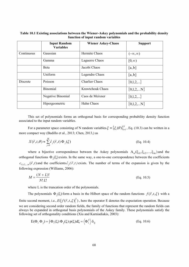
68

Table 10.1 Existing associations between the Wiener-Askey polynomials and the probability density function of input random variables

Input Random Variables

Wiener Askey-Chaos Support

Continuous Gaussian Hermite Chaos ),( ∞−∞

Gamma Laguerre Chaos ),0[ ∞

Beta Jacobi Chaos ]b,a[

Uniform Legendre Chaos ]b,a[

Discrete Poisson Charlier Chaos ,...2,1,0

Binomial Krawtchouk Chaos N,...2,1,0

Negative Binomial Caos de Meixner ,...2,1,0

Hipergeometric Hahn Chaos N,...2,1,0

This set of polynomials forms an orthogonal basis for corresponding probability density function associated to the input random variables.

For a parameter space consisting of N random variables Nii 1)( =≡ θξξ , Eq. (10.3) can be written in a

more compact way (Badillo et al., 2013; Chen, 2013,) as

∑=

Φ≈M

jjj trctrX

0)(),(ˆ),,( ξθ

(Eq. 10.4)

where a bijective correspondence between the Askey polynomials ),...,,(A in2i1in ξξξ and the orthogonal functions )(j ξΦ exists. In the same way, a one-to-one correspondence between the coefficients

),(,...2,1 trc inii

and the coefficients )t,r(c j

exists. The number of terms of the expansion is given by the following expression (Williams, 2006):

!!)!(

LNLNM +

= (Eq. 10.5)

where L is the truncation order of the polynomials.

The polynomials )(j ξΦ form a basis in the Hilbert space of the random functions ),,( ξtrf with a

finite second moment, i.e., )),,(( 2ξtrfE , here the operator E denotes the expectation operation. Because

we are considering second order random fields, the family of functions that represent the random fields can always be expanded in orthogonal basis polynomials of the Askey family. These polynomials satisfy the following set of orthogonality conditions (Xiu and Karniadiakis, 2003):

ij2ijiji d)(p)()()(E dΦ=ξξξΦ∫ ξΦ=ΦΦ (Eq. 10.6)

69

where )(p ξ is the PDF of ξ and ijd the Kronecker delta. In practice, the polynomial type is chosen in such a way that the weighting function of these polynomials is the same one as for the PDF of the random variables that enter into the problem. For instance, the Laguerre polynomials with support ),0[ ∞ have an exponential weighting function, while the associated Laguerre polynomials have the gamma distribution as the weighting function.

In the case that we have several stochastic input variables that follow different probability distributions, the polynomials to be used are different for each variable. For example, for the case of the two variables 1ξ and 2ξ , if we denote the polynomials for the first variable by )( 1ξφi and the polynomials for the second variable with )( 1ξψ j , the new basis is formed by the tensorial product

)()( 21),( ξψξφ jijik ⊗=Φ . The inner product of these basis functions is defined by

∫∫=ΦΦ 2222'2111'1)','('),( )()()()()()(, ξξξψξψξξξφξφ dpdp jjiijikjik (Eq. 10.7)

where the basis polynomials are now different for each variable but the GPCE has a similar structure (Badillo et al., 2013):

...),,( 202,0111,1020,2101,0010,1000,0 ++++++= ψφψφψφψφψφψφθ cccccctrX (Eq. 10.8)

As previously, we can write the stochastic random field as follows:

∑=

Φ≈M

kjikjik trctrX

0),(),( )(),(ˆ),,( ξθ (Eq. 10.9)

The GPCE method applied to the Navier-Stokes equations by intrusive methods

Two alternatives to apply the GPCE to the Navier-Stokes equations exist. The first one is based on an intrusive method that is not suitable for commercial codes such as ANSYS-CFX but is applicable to open source codes such as Open-FOAM. In the intrusive methods, a set of coupled Navier-Stokes-like equations, whose numerical solution requires changes in the solver, is obtained.

The starting point for the derivation of the stochastic hydrodynamic equations is the incompressible Navier-Stokes (Xiu and Karniadakis, 2003):

0u. =∇

(Eq. 10.10)

( ) uRepu.utu 21

∇+∇−=∇+∂∂ − (Eq. 10.11)

where p and u denote the pressure and velocity fields, respectively. These equations are transformed into stochastic conservation laws by assuming that the physical quantities p and u are stochastic processes depending on the random parameter Ω∈θ . These stochastic random fields are then defined by the family of functions:

);,( θtruu = (Eq. 10.12)

);,( θtrpp = (Eq. 10.13)

70

The next step is to perform a GPCE with Askey polynomials assuming that there is a finite number of stochastic variables N

1ii )( =θξ , where the M is the number of terms of this expansion and depends on N number of stochastic variables and the truncation order L of the Askey polynomials. In general one can write

∑≈−

=

1M

0iii ))(()t,r(u);t,r(u θξΦθ

(Eq. 10.14)

∑≈−

=

1M

0iii ))(()t,r(p);t,r(p θξΦθ

(Eq. 10.15)

where ),( trui

and ),( trpi

are coefficients of GPCE.

The most interesting aspect of the expansions Eqs. (10.14) and (10.15) is that by means of these GPCEs the stochastic processes are decomposed in a set of deterministic functions ),( trui

and ),( trpi

and

multiplied by the basis polynomials 10−

=Φ Mii that are independent of the space-temporal variables )t,r(

and depend on the stochastic variables of the fields. Replacing these expansions into the Navier-Stokes leads to the following equation:

0))((u. ii1M

0i=∇∑

−

=θξΦ

Eq. (10.16)

( )[ ] ( ) i

M

iii

M

ii

M

i

M

jjijii

M

i

i upuut

txuΦ∇+Φ∇−=ΦΦ∇+Φ

∂∂

∑∑∑ ∑∑−

=

−−

=

−

=

−

=

−

=

1

0

211

0

1

0

1

0

1

0Re.))((),(

θξ (Eq. 10.17)

Projecting Eqs. (10.16) and (10.17) onto the basis functions ))((k θξΦ

yields

1,...1,00. −==∇ Mkuk

(Eq. 10.18)

( )[ ] ( )k21

k1M

0i

1M

0jjiijk2

k

k uRepu.ue1t

)t,x(u

∇+∇−=∑ ∑ ∇+∂

∂ −−

=

−

=Φ (Eq. 10.19)

where the coupling coefficient is given by

kjiijke ΦΦΦ= (Eq. 10.20)

This set of M Navier-Stokes-like equations are coupled through the convective terms ijke and

jiΦΦ . The coupling coefficient ijke can be computed analytically and depends on the type of polynomials and their truncation order defined by the indices i,j,k. These equations can be solved by conventional numerical methods used in CFD (e.g. finite difference, finite elements, finite volume). Since

),( trui

and ),( trpi

are the coefficients of the GPCE, the mean velocity and pressure fields are given by the zeroth order coefficient, which is

),(),( 0 trutru = (Eq. 10.21)

),(),( 0 trptrp = (Eq. 10.22)

71

The second moment or cross-covariance between two points can be obtained as follows:

)),(),(()),,(),((),;,( 22022110112211 trutrutrutrutrtrRuu

−−= , (Eq. 10.23)

which on account of the orthogonality property of the polynomials can be expressed in the form:

22

1

12112211 ),(),(),;,( i

M

iiiuu trutrutrtrR Φ= ∑

−

=

(Eq. 10.24)

The variance is given by

[ ]∑−

=Φ=−=

1

1

2220 ),()),(),((),((

M

iii trutrutrutruVar (Eq. 10.25)

The GPCE method applied to CFD by non-intrusive methods

In the non-intrusive GPCE collocation method used by Simon et al. (2010) and Badillo et al. (2013), a pseudo spectral expansion is used. The method relies on evaluating the solution at a finite number of collocation points, or samples, where relevant measures such as mean and standard deviation fields are obtained during a post-processing stage based on the solver evaluation. In this approach, the solver must be executed Nsamples times, varying the input stochastic variables in their respective support intervals. In the example that follows, we assume only two random input variables, i.e. 21,ξξξ = . Proceeding in this way,

we obtain the pressure samplesNiirp 1),( =θ and the velocity samplesN

iiru 1),( =θ fields at a set of collocation points of the random variables. Then one can obtain the coefficients of the expansion from the projection definition as in Simon (2010):

))((

))((),()(

2 θξ

θξθ

j

jj

rprp

Φ

Φ=

(Eq. 10.26)

with

))(())(,(1))((),(1

ljl

N

lsamplesj rp

Nrp

samples

θξθξθξθ Φ=Φ ∑=

(Eq. 10.27)

As in the intrusive methods, the statistical moments up to second order can be computed in terms of the coefficients of the GPCE as

)(),( 0)( rprprp

== θµ (Eq. 10.28)

and the variance

∑−

=Φ=−=

1

1

2220

2)( )())(),((

M

jjjrp rprprp

θσ (Eq. 10.29)

This method is non-intrusive in the sense that it projects the stochastic solution directly onto the members of the orthogonal basis chosen to span the random space. The expansion coefficients can be calculated as in Badillo et al. (2013) to solve the following system of equations:

( ) ( )

( ) ( )

=

ΦΦ

ΦΦ

−−

−

)(

)( 00

1

0

10

0100

NsamplesNsamplesMNsamplesMNsamples

M

X

X

c

c

ξ

ξ

ξξ

ξξ

(Eq. 10.30)

72

If the number of collocation points Nsamples is larger than the number of coefficients M, the system is over-determined, and an optimisation procedure is required to solve Eq. (10.30). The total number of random variables that can be handled simultaneously with polynomial chaos expansions (PCEs), depends only on the computational power available for the calculations. Eq. (10.5) presents the minimum number of calculations required to calculate the PCE coefficients for a given truncation order and number of random variables. As an example, if we consider six random variables 6=n and a truncation order 4=p , the minimum number of simulations is 210=M . By decreasing the order of the polynomial chaos to 2=p , the number of simulations required is significantly reduced to 28=M , but the truncation error increases.

10.3 Some results of CFD uncertainty calculations using the non-intrusive GPCE method

The water mixing experiments conducted in the GEMIX-Facility (GEneric MIxing eXperiment) at the Paul Scherrer Institute focus on the basic mechanisms of turbulent mixing in the presence of temperature and/or density gradients under isokinetic mixing conditions. To study the fundamental mixing phenomena, co-flow experiments were carried out in a square channel with Reynolds numbers covering the range of Re = 5,000 to 60,000 at various relative densities (Metzner et al., 2006, Badillo et al., 2013). This section is devoted to the study of the uncertainty of the results obtained with ANSYS-FLUENT when simulating these experiments (see Figure 10.2).

Strictly speaking, stochastic variables can be introduced in a deterministic system only when a variable or parameter displays a certain degree of randomness, characterised by a probability density distribution. Nonetheless and as explained before, in a Bayesian framework, a probability density distribution representing the degree of belief in a proposition could also be assigned to a variable whose precise value is not known. Based on this idea, random parameters have been introduced to account for the variability of the inlet boundary conditions and of the turbulent Schmidt number (either epistemic or aleatoric) on the turbulent mixing of two fluids in a square channel. Despite the fact that the GEMIX experiment is well instrumented in the mixing section, velocity profiles and turbulence quantities were not measured in the inflow section. Although honeycombs and grids of different sizes were placed in the inflow section in an attempt to decrease the level of turbulence and propitiate a uniform velocity profile, accurate velocity profiles and turbulent quantities are not known at the location of the finest grid, which coincides with the inlet of our numerical setup (see Figure 10.3). Thus, only the mass flux at the inlet is known.

Figure 10.2: Schematic of the GEMIX experiment and inflow section of the GEMIX facility

In order to treat the uncertain boundary condition at the inlet, the velocity profile has been parametrised and assumed to be in between a fully developed (turbulent) and a uniform velocity profile. In

addition, turbulent quantities are described solely by the turbulence intensity 232 Uk=β , where k is the turbulence kinetic energy and U the mean velocity field. The velocity profile controlled by a single parameter α is given by

73

( ) ( )

11,

−

−+=

ud uyuyu ααα , (Eq. 10.31)

where the sub-indexes d and u stand for developed and uniform, respectively. Eq. (10.14) yields an interpolated velocity profile that satisfies the non-slip condition at the wall for ( )1,0∈α . In the present work, a uniform probability density distribution was assigned to all random variables.

1.1.2. Simulation conditions

One of the main objectives of this section is to present a simple methodology to quantify the uncertainty propagation, using non-intrusive techniques along with a commercial CFD package. The commercial software selected for this purpose was ANSYS-FLUENT© V.13 (publisher, year). All the simulations performed to quantify uncertainty propagation considered the standard ε−k model with default values for all the coefficients, meaning the same holds for the models used to estimate the variability in the results arising from the selection of turbulence model. In addition, scalable wall functions were used to properly calculate the velocity field at the splitter plate where y+ is around 10. The mesh consists of 475’200 nodes (see Figure 10.3), and the SIMPLE algorithm was used to link the momentum and mass conservation equations. A second order upwind scheme was used to calculate the advection terms for all the variables. The mass flux at the inlet was equal to 1 kg/s in each leg, which translates to a velocity of 0.8 m/s, considering a uniform velocity profile and a density of 998 kg/m3 for water at T = 23°C.

Figure 10.3: Computational mesh with the numbers indicating the number

of nodes in each direction

The quantification of the inlet uncertainty was carried out by fixing the turbulent Schmidt number at 7.0=Sc and running 88 simulations, where the parameter α controlling the shape of the velocity profile

and the turbulence intensity β were varied independently in a rectangular arrangement (see Figure 10.4). The fully developed velocity profile was obtained by an independent simulation in a small portion of the upper leg in the inflow section, considering periodic boundary conditions at the inlet and outlet. The support interval – where the variables are thought to be physically possible – was ( ) [ ] [ ]4,01,0, ×∈βα . In Figure 10.4, the points enclosed by red circles show a possible distribution which could provide similar results with a much lower number of simulations. In practice, 15 collocation points (if selected properly) should suffice, but in the present work, the regular matrix composed of 88 points will serve to investigate the dependence of the results on the configuration. These results will be presented in a forthcoming publication, along with the convergence of the PCE as a function of the polynomial order. To evaluate the influence of the variation of the turbulent Schmidt number, defined as the ratio between the turbulent kinematic eddy viscosity and the turbulent diffusion coefficient turbeddy DSc ν= , a combination of

74

5.0=α and 2=β was fixed, and only seven collocation points 3.1,0.1,9.0,7.0,5.0,3.0,1.0=Sc were chosen in the support interval [ ]3.1,1.0∈Sc . In all the calculations, the PCEs were truncated at the fourth order.

1.1.3. Results

The combined effects of the uncertainty in the coefficient α and the turbulence intensity β at the inlet are shown in Figure 10.5. Mean values look similar to those obtained from deterministic simulations, but relevant insight is gained by the additional information provided by standard deviation. For the velocity field, the highest values for σ are found right at the inlet, but that is not the case for the turbulent kinetic energy. For turbulent kinetic energy, the highest values are located inside the inflow section, which is a counterintuitive result. The mixing scalar (concentration) displays the highest standard deviation at the channel outlet, which can be explained in terms of the variability of the turbulent kinetic energy and the residence time of the fluid inside the channel. Since the turbulent diffusion coefficient is related to the turbulent kinetic energy through the Schmidt number and the turbulent kinematic eddy viscosity, the variability in the turbulent kinetic energy induces variability in the diffusion time along the channel. Hence, the longer the residence time inside the mixing section, the higher the variability (standard deviation) in the distribution of the mixing scalar.

A comparison of the calculated mean velocity and turbulent kinetic energy profiles with the experimental measurements is presented in Figure 10.6. Figure 10.7 shows the level of uncertainty introduced either by the inlet boundary conditions (left) or by the turbulent Schmidt number (right) on the mean concentration profiles.

The change in the shape of the turbulent mixing layer upon variation of Sc is presented in Figure 10.8, where the green colour signifies a concentration from 0.1 to 0.9. Figure 10.9 displays the mixing scalar field (concentration) and its associated standard deviation at the centre plane. Compared to the uncertainty introduced by the inlet boundary conditions, the standard deviation related to the variability of Sc is higher, but its overall distribution is similar. This is largely because the turbulent mixing for low Schmidt numbers (less than 0.3) is very high. With the selection of a normal probability distribution for Sc (with a mean value equal to Sc = 0.7), the large contribution to the errors bars from low Sc numbers can be attenuated if the standard deviation of the proposed distribution is small. Nonetheless, additional information is required to construct the appropriate probability distribution. Results evaluating several probability distributions for Sc will be presented in a forthcoming publication.

Figure 10.4: Collocation points for the coefficient controlling the velocity profileα

and turbulence intensityβ

The variability in the results introduced by the turbulence model is mild compared to uncertainties introduced by the inlet boundary conditions or the turbulent Schmidt number. Figure 10.10 shows the

75

velocity, turbulent kinetic energy, and concentration profiles at two locations inside the mixing section obtained using the standard ε−k , realisable−− εk , ω−k , SSTk −−ω , and RSM. Concentration and turbulent kinetic energy distributions at the outlet are presented in Figure 10.10. Slight differences are observed in the concentration distribution at the outlet; however, the distribution predicted by RSM resembles the experimental results more closely (not shown in this paper). The turbulent kinetic energy predicted by RSM also departs from the other models, especially close to the walls. Despite mild differences in the results, the evolution of the thickness of the turbulence mixing layer along the channel is well captured by all the models.

Figure 10.5: Stochastic CFD results for turbulent mixing: Mean values and standard deviation for the

most relevant quantities are shown at the centre plane of the computational domain.

76

Figure 10.6: Mean velocity and turbulent kinetic energy: Error bars correspond to a 1± standard deviation and consider only the variability in the inlet boundary condition.

Figure 10.7: Dimensionless mean concentration profiles: The effects of uncertain inlet boundary conditions

and turbulent Schmidt numbers are presented on the left and right, respectively.

Figure 10.8: Influence of the turbulent Schmidt number on the shape of the mixing layer: Each figure shows the results of a deterministic simulation for 5.0=α and 2=β . The green colour represents a

concentration range from 0.1 to 0.9.

mm70=x mm450=x

77

Figure 10.9:The dimensionless mean concentration and standard deviation for a stochastic Schmidt

number: The results were obtained by using PCE to combine the seven simulations.

Figure 10.10: Deterministic profiles at the centre plane for five turbulence models. All simulations

considered 5.0=α , 2=β , and 7.0=Sc .

Figure 10.1:– The crosswise dimensionless mean concentration (left) and the turbulent kinetic energy maps (right) at the outlet obtained with five turbulence models

78

10.4 Conclusions

In this section, we have the intrusive and non-intrusive GPCE methods for quantifying the uncertainty in stochastic random fields. These methods are a well-established and robust techniques that allows for the evaluation of the uncertainty in complex CFD models. However, when using commercial packages, it is not possible to modify the source code, and consequently, mostly non-intrusive methods can be used.

The determination of the input and model parameters that have the strongest influence on the output results must be estimated previously by well-known, established techniques such as PIRT and sensitivity analysis. In the previous example, we have seen that the results are not sensitive to the turbulence model as displayed in Figure 10.10.

LES simulations have proven to produce accurate results in the description of mixing processes such as those in T-junctions. Nonetheless, LES simulations still pose an important computational burden for more complex systems. Consequently, turbulence models based on RANS equations constitute a cost-effective alternative to calculate flow fields in larger systems or problems where a large number of parameters needs to be varied.

In this document, stochastic-CFD simulations of the turbulent mixing of water in the GEMIX facility were accompanied by PCE to quantify the errors introduced by uncertainties in (i) the shape of the inlet velocity profiles (uniform versus fully developed), (ii) the level of the turbulence intensities, and (iii) the turbulent Schmidt number. The simulations revealed that a better agreement with the experimental results can be achieved by the introduction of stochastic variables controlling the shape of the velocity profile and turbulence intensity at the inlet ( )βα , as well as the turbulent diffusion (stochastic turbulent Schmidt number). Further we showed that the choice of the turbulence model has only a mild influence on the mixing experiments considered here when compared with the level of uncertainties introduced by the inlet boundary conditions or the turbulent Schmidt number. While the former is not directly accessible through measurements in the GEMIX facility, researchers have strongly recommended to measure the inlet conditions whenever possible to form a complete data set. Both worlds – experimental and simulation – will profit from this.

10.5 Characteristics of the method

PCE is a propagation method. PCEs are recognised as a meta-model in the sense that the response is represented by a linear combination of polynomials. Nonetheless, the selection of the orthogonal polynomial basis depends on the PDF of the input random parameters. In contrast to conventional propagation methods using meta-models in which the interpolating polynomials have no relation to the inputs, the propagation step in PCE does not require the use of Monte Carlo methods applied to the interpolated response surface. To obtain the appropriate moments for the output (mean, standard deviation, etc.), we make use of the orthogonal property of the polynomials and calculate the statistical moments from the polynomial coefficients. This method also allows for a rigorous sensitivity analysis in terms of the Sobol’s indices.

PCE does not constitute a complete UQ methodology; it is only a propagation method. Being a probabilistic propagation method, it can address any type of uncertainty as long as the uncertainty is represented by a PDF. Epistemic uncertainties due to incomplete physical models can be treated in a Bayesian probability framework, where the PDFs of input parameters are constructed from expert judgement and available quantitative information.

If we treat all numerical options with a uniform PDF, then in principle, we could include uncertainty due to numerics in the analysis.

This method can address uncertainty due to geometric simplification depending on how this input uncertainty is represented. To assess the level of uncertainty introduced by unresolved scales (geometrical, turbulent, etc.), we must have the appropriate data including all the unresolved details. If this information

79

is available, then a PDF could be constructed and propagated through the simulations.

We are using PCE applied to CFD, and therefore, scalability is not an issue. Nevertheless, the level of uncertainty introduced by uncertain boundary and initial conditions, turbulence closure laws, and numerical errors can vary substantially from small to large scales. In fact, the main reason for large discrepancies between CFD simulations and experiments is most probably due to numerical errors rather than to turbulence closure laws, which are derived using physical arguments at small size and time scales; turbulence model coefficients and wall functions do not depend on the system’s size.

Neither SET data nor IET data are used in the propagation step.

There is no code calibration for data in the propagation phase.

The number of reactor calculations depends on the number of input parameters and the degree of the polynomials. Selecting second order polynomials and seven random parameters, we need 36 simulations. Increasing the polynomial degree to four would require 330 simulations for the same number of parameters. Systematic observations show that only low degree polynomials contribute considerably to the solution.

As mentioned before, PCE is not a complete UQ methodology but only a propagation method, and as such, well established and with a high degree of maturity.

80

81

11. METHODS FOR NUMERICAL ERROR EVALUATION

When a discretised solution is sought for a system of equations, numerical error naturally arises due to discretisation in space and time. With decreasing mesh size or time step, the error also decreases. The goal of solution verification is to estimate the magnitude of the error and provide an interval within which the exact solution will be found with a certain level of confidence. These two distinct steps of analysis are described below.

11.1 Error estimation

Two commonly used methods for the error magnitude estimation are the Richardson extrapolation (RE) and the least-squares (LS) method. RE was first introduced in 1910, and the modified RE provides the most general solution. RE works well when the solution response is monotonic with respect to mesh size but may lead to unexpected results when the response is not monotonic. In such cases, the LS method provides an improved solution.

In both methods, the convergence of the numerical solution with decreasing mesh size is analysed. However, one needs to ensure that the mesh size remains small enough to resolve the physical phenomena one attempts to resolve.

The values of the analysed numerical solution should be free of iteration errors and boundary effects. One needs to ensure that the iteration error is 2 to 3 orders of magnitudes smaller than the discretisation error. If that is not the case, the two errors are combined in a conservative manner such that unum = uh + ui, where ui is the iteration error, uh the discretisation error, and unum the numerical uncertainty. The analysed solution value should also be taken at a location that has minimal boundary effects.

If transient effects in the model physics strongly influence the analysed numerical solution, both RE and LS methods may have poor convergence because of the physical effects. In such cases, integral measures such as the lift coefficient can lead to better convergence in the numerical errors.

Both the RE and LS methods are described below.

11.2 The Richardson extrapolation

Richardson supposed that a numerically discretised solution 𝜑𝜑 could be expressed as a limited development in terms of the grid spacing h : 𝜑𝜑 = 𝜑𝜑𝑚𝑚𝑒𝑒𝑣𝑣𝑒𝑒𝑡𝑡 + 𝛼𝛼ℎ𝑖𝑖 + ⋯ . If the algorithm’s order of accuracy, denoted as 𝑝𝑝 in the limited development above, is known, then only two unknowns are in this development: 𝜑𝜑𝑚𝑚𝑒𝑒𝑣𝑣𝑒𝑒𝑡𝑡 and 𝛼𝛼. Consequently, the value of 𝜑𝜑𝑚𝑚𝑒𝑒𝑣𝑣𝑒𝑒𝑡𝑡 can be determined by using two solutions with different grid sizes. If the order of accuracy is not known, a minimum of three solutions with different grid sizes is needed.

The analysis steps outlined by ASME are as follows:

1. A representative mesh size is defined. If a 3D mesh is structured and isotropic, a characteristic mesh size is determined from [ ] 3/1

maxmaxmax zyxh ∆∆∆= where the maximum mesh size in each Cartesian direction is used. If the mesh is not structured, the characteristic

82

mesh size can be estimated from [ ] 3/1/ NVh TOTAL= where TOTALV is the total mesh volume and 𝑁𝑁 is the number of cells.

2. Several significantly different mesh sizes are selected for simulations. Typically, a refinement by a factor of two and an enlargement by a factor of two are chosen with respect to the reference solution, giving mesh size ranges of [1 2h, h, 2h, 4h⁄ ], but the scaling ratio can be different for different grids. Although an integer scaling ratio is desirable, it is not required. However, based on empirical experience, ASME (2009) recommends a ratio of r =hcoarse

hfine greater than 1.3. The grid refinement should be performed isotropically in all

Cartesian directions.

3. With three different mesh sizes, 1h , 2h , and 3h , and h1 < h2 < h3, one can write the following three equations:

𝜑𝜑1 = 𝜑𝜑𝑚𝑚𝑒𝑒𝑣𝑣𝑒𝑒𝑡𝑡 + 𝛼𝛼ℎ1𝑖𝑖 + +0ℎ1

𝑖𝑖+1

𝜑𝜑2 = 𝜑𝜑𝑚𝑚𝑒𝑒𝑣𝑣𝑒𝑒𝑡𝑡 + 𝛼𝛼ℎ2𝑖𝑖 + +0ℎ2

𝑖𝑖+1

𝜑𝜑3 = 𝜑𝜑𝑚𝑚𝑒𝑒𝑣𝑣𝑒𝑒𝑡𝑡 + 𝛼𝛼ℎ3𝑖𝑖 + +0ℎ3

𝑖𝑖+1

One defines the ratios 𝑟𝑟21 = ℎ2 ℎ1⁄ and 𝑟𝑟32 = ℎ3 ℎ2⁄ . In the simple case where both ratios are equal, one easily calculates analytically that

𝑝𝑝 =𝑙𝑙𝑛𝑛 𝜑𝜑3 − 𝜑𝜑2

𝜑𝜑2 − 𝜑𝜑1

𝑙𝑙𝑛𝑛 (𝑟𝑟)

and

𝜑𝜑𝑚𝑚𝑒𝑒𝑣𝑣𝑒𝑒𝑡𝑡 = 𝜑𝜑1 −𝜑𝜑2−𝜑𝜑1𝑟𝑟𝑝𝑝−1

ASME (2009) proposes an extrapolation of these formulas for the case where 𝑟𝑟21 and 𝑟𝑟32 are different. The differences between the successive solutions iϕ , denoted as 2332 ϕϕε −= and

1221 ϕϕε −= and the apparent order of the accuracy, 𝑝𝑝, can be determined from:

( )2132 / εεsigns = ,

−−

=srsrpq p

p

32

21ln)( ,

[ ][ ] 0)(/ln)ln(/1 213221 =+− pqrp εε .

The value 𝑝𝑝 is solved iteratively from an initial guess until the following condition is met for a small value of ε :

[ ] εεε <

−

−+− ∗

∗

∗

srsrrp

p

p

32

21213221 ln/ln)ln(/1 .

However, if the mesh refinement ratio 𝑟𝑟 is constant, then 𝑞𝑞(𝑝𝑝) = 0 , and the solution is simplified. This step is omitted if the apparent order of convergence is known.

83

4. Once 𝑝𝑝 is determined, one can calculate the extrapolated value of the solution from )1)(( 212121

21 −−= ppext rr ϕϕϕ . The normalised relative error is determined using

1

2121

ϕϕϕ −

=ne and the estimated extrapolation error from 211

2121

ext

extexte

ϕϕϕ −

= . In the ASME

report, the above methodology is implemented using three solutions with three different mesh sizes. An implementation with more than three solutions was not discussed, but one could easily imagine repeating RE with all possible 3-element subsets of all solutions. However, the result from the subset containing the three finest meshes will likely be the most accurate.

11.3 Least-squares approach

When the convergence of the numerical solution with decreasing grid size is monotonic, the LE approach as proposed by Eca and Hoekstra (2002) can be used to determine the numerical error. In this approach, a minimum of four grid points is needed for solutions whose convergence is evident, but at least six grid points may be required to obtain stable results for solutions with poor convergence.

We assume that the numerical solution is different from the exact solution by a factor of the grid difference 𝜑𝜑𝑖𝑖 − 𝜑𝜑∞ ≅ 𝛼𝛼ℎ𝑖𝑖

𝑖𝑖. The LE approach aims to minimise the difference between the ith numerical results 𝜑𝜑𝑖𝑖 and its best-fit of the convergence 𝜑𝜑∞ + 𝛼𝛼ℎ𝑖𝑖

𝑖𝑖. The sum of the total error is

( )[ ]∑=

∞∞ +−=n

i

pii hpS

1

2),,( αϕϕαϕ ,

where 𝑛𝑛 is the number of solutions. The minimum solution is found by finding the roots of the three equations: partial derivatives of ),,( pS αϕ∞ with respect to ∞ϕ , α , and p = 0. Solving these 3 equations leads to

−

−

=

∑∑

∑∑∑

==

===n

i

pi

n

i

pi

n

i

pi

n

ii

n

i

pii

hhn

hhn

11

2

111

2

ϕϕα ,

−= ∑∑==

∞

n

i

pi

n

ii h

n 11

1 αϕϕ ,

∑∑∑==

∞=

∞ −−=∂

∂ n

ii

pi

n

ii

pi

n

ii

pii hhhhhh

ppS

1

2

11)log()log()log(),,( αϕϕαϕ = 0

The solution is determined iteratively by a false position method for the value of p .The value of α

is determined before it is substituted into the equation for ∞ϕ .The value p

pS∂

∂ ∞ ),,( αϕ is determined from

the derived α and ∞ϕ , and the value of p is sought iteratively until p

pS∂

∂ ∞ ),,( αϕ becomes smaller than

the target value.

84

If the calculated value of p is larger than the theoretical value, the theoretical maximum is used

instead. The value of α which yields 0),,(=

∂∂

∞

∞

ϕαϕ pS is then determined, allowing the value of ∞ϕ to

be evaluated.

11.4 Uncertainty estimation

The final goal of solution verification is to estimate an uncertainty range, i.e., f ± Uα, such that one has a likelihood of α that the exact solution is within this range. The typical value of the likelihood used is α = 95%, which is comparable to two standard deviations of a standard Gaussian random variable.

The ASME report proposed an estimation of the uncertainty range by the grid convergence index (GCI) (Roache, 1998). In GCI, the U95% uncertainty range is given by multiplying the numerical error with a factor of safety, Fs . This conversion from numerical error to numerical uncertainty is made and verified through repeated empirical observations. The value of Fs depends on the behaviour observed in mesh convergence studies. Fs is larger if only a few mesh sizes are studied or if the convergence behaviour is erratic.

The GCI based on the solution with the finest mesh is

121

2121

−⋅

= pn

fine reFsGCI where one recalls that

1

2121

ϕϕϕ −

=ne .

The value of Fs is determined according to the quality of the available solutions. In general, if the grid convergence is smooth and many solutions are available, we use a less-penalising value of 1.25. In contrast, if the grid convergence is erratic and few solutions were done, a more penalising value of 3.0 is used to increase the magnitude of the estimated numerical standard deviation (Table 11.1).

Table 11.1: Different value of factors of safety for estimation of grid convergence index

Fs Conditions Applicable Method

1.25 at least three grids Richardson extrapolation, without known p

3.00 two grids Richardson, with known p

1.25 at least four grids least-square

3.00 at least four grids, least-square, with erratic convergence

The estimation of Fs is a controversial topic. Several improvements have been proposed to take into account that the estimated order of accuracy is sometimes different from the theoretical one (Xing and Stern, 2010). The proposed factors of safety are validated on numerous cases where the exact value of the solution is known, either because the considered case has an analytical solution or because an experimental value of the solution is available.

Once the GCI is calculated, the numerical uncertainty unum can be estimated. GCI is an estimation of the 95%-interval of variation of the exact solution while in the ASME VVUQ standard, the numerical uncertainty is given by one standard deviation. To reconcile these two values, ASME proposed a conversion. When the grid convergence of the solution is erratic, ASME assumes that, at best, the

85

distribution of the numerical error can be centred on the finest solution. If the distribution is Gaussian, the conversion from GCI to unum is as follows because GCI is an estimate of two standard deviations:

unum = GCI/2.

If the grid convergence is smooth, the distribution of the numerical error will be centred on the extrapolated solution. The estimation of unum, which is centred on the finest solution, will be based on a shifted Gaussian hypothesis and, consequently, will use a more penalising conversion of

unum = GCI/k

where k has a value between 1.1 and 1.15.

86

87

12. BRIEF DESCRIPTION OF TWO PROCEDURES TESTED IN EDF

This section presents methods developed and tested at Électricité de France (EDF)

12.1 Univariate uncertainty quantification

12.1.1 General presentation

The purpose of the method named Weighing Approach for Validation against Experiment (WAVE) is to produce, for a certain quantity of interest S (S being a scalar output of the CFD calculation performed at reactor scale), a value S5/95 that is smaller (or greater, depending on what is penalising) than 95% of the possible values of S with a confidence level of 95%. The confidence level comes from the finite number of experimental test cases at one’s disposal. This method, as with some other VVUQ approaches, is based on a comparison between experimental results and calculation results at the test case scale. It also considers propagation of the uncertainty of input data parameters.

12.1.2 Notation

S is the scalar quantity of interest; for example, S is a fluid temperature during a PTS transient at a given location in space and time. In the following, we assume that S is made non-dimensional in an appropriate way so that values at reactor scale and at test case scale can be compared directly.

The following definitions are what we use in this work:

• St is the “true” (unknown) value of S.

• SCFD is the value of S calculated by the CFD model.

• “r” represents the true (unknown) conditions at reactor scale

• “R” represents the best estimate value of “r”.

Thus, St(r) is the “true” (unknown) value of S at reactor scale; SCFD(R) is the result of the CFD calculation at reactor scale; SCFD(r) is the result a CFD calculation would produce for the “true” reactor scale conditions (if these conditions were known).

Similarly, “e” represents the “true” (unknown) conditions at test case scale; “E” represents our estimation of “e”. Since several experimental tests are used in the method, index “k” is used to differentiate these K tests.

Thus, St(ek) is the (unknown) true value of S in test number k; SCFD(Ek) is the result of the CFD simulation of test number k; SCFD(ek) is the result a CFD calculation would produce for the “true” test number k conditions, if these conditions were known.

We also introduce the following notations:

• mk is the “true” value of S in experimental test number k, i.e., mk= St(ek).

• Mk is the measured value of S in experimental test number k. When measuring mk, the answer we get is Mk, because instrumentation has a limited accuracy.

88

12.1.3 Mathematical formulation

At reactor scale, we write that the “true” value of S can be split as follows:

St(r) = (St(r) – SCFD(r)) + (( SCFD(r) - SCFD(R)) + SCFD(R)) (Eq. 12.1)

On the right-hand side of this equation, the first term represents “how wrong” the CFD model is at reactor scale. We note this term “A”. This term is intrinsic to the model: the “true” reactor scale conditions “r” appear here, so no uncertainty of these conditions is present in “A”.

The second term is the result of the CFD calculation at reactor scale SCFD(R) plus a correction due to our imperfect knowledge of the true reactor scale conditions. We note this term “B”.

We thus have St(r) = A + B.

St is the “true” value of S at reactor scale. We are now going to represent our knowledge of St with a random variable based on the splitting above:

• The random aspect of B simply means that our knowledge of the true conditions at reactor scale is imperfect. “R” represents “r” with some uncertainty, and this uncertainty is propagated through the CFD model.

• The random aspect of A is based on the way we estimate this term, which is detailed below.

At this point, how can we get some knowledge of term A, that is, of “how wrong” the model is? In the method, this knowledge is based on the comparison of model results with experimental results obtained at test case scale, the test case being a good representation of the reactor. A hypothesis in this method is the “scalability hypothesis” which states that model error at reactor scale is assumed equal to model error for the simulation of an experimental test k at test case scale. This hypothesis has to be justified by preliminary work with a PIRT and validation experiments. Of course, this result does not come from rigorous mathematical proof, but by relying on concrete physics-based reasons, one can expect a reasonable value.

With this hypothesis, term A is taken equal to a term Ak (for a given test k), which verifies

Ak= St(ek) – SCFD(ek) (Eq. 12.2)

Ak= (St(ek) – SCFD(Ek)) + (SCFD(Ek) – SCFD(ek)) (Eq. 12.3)

We can introduce the measured value of S in this formula:

Ak= (St(ek) – Smeasured(ek)) + (Smeasured(ek) – SCFD(Ek)) + (SCFD(Ek) – SCFD(ek)) (Eq. 12.4)

Or we can use the notations introduced above in section 12.1.2:

Ak= (mk – Mk) + (Mk – SCFD(Ek)) + (SCFD(Ek) – SCFD(ek)) (Eq. 12.5)

On the right-hand side of Eq. (12.5),

• the first term stands for measurement error,

• the second represents the difference we obtain between measurement and calculation results at test case scale,

• the third shows the impact our imperfect knowledge of the true conditions at test case scale has on the calculation result; this term is similar to the corresponding term at reactor scale, which is present in the expression of B.

With the “scalability hypothesis”, St can be written as a sum of calculable terms:

St,k(r) = Ak + B (Eq. 12.6)

89

St,k(r) = (mk–Mk)+(Mk–SCFD(Ek))+(SCFD(Ek)–SCFD(ek))+((SCFD(r)-SCFD(R))+SCFD(R)) (Eq. 12.7)

At this step, the CFD result at reactor scale is considered unique. Yet, different numerical parameters can vary between validation and reactor calculation (e.g. mesh, time step, numerical scheme) within the range of BPGs and V&V. These different numerical configurations induce variability in the CFD results. For practical reasons, we suggest treating this variability at test case scale. A new notation is introduced using index “CFD” with the number “1” corresponding to test case scale simulation with numerical parameter set number 1, number “2” corresponding to a second set of numerical parameters, and so on. A new term appears in Eq. (12.7), which leads to the following equations:

𝑆𝑆𝑡𝑡,𝑘𝑘(𝑟𝑟) = (𝑚𝑚𝑘𝑘 −𝑀𝑀𝑘𝑘)

+ (𝑀𝑀𝑘𝑘 − 𝑆𝑆𝐶𝐶𝐶𝐶𝐷𝐷1(𝐸𝐸𝑘𝑘))

+ (𝑆𝑆𝐶𝐶𝐶𝐶𝐷𝐷1(𝐸𝐸𝑘𝑘)− 𝑆𝑆𝐶𝐶𝐶𝐶𝐷𝐷1(𝑒𝑒𝑘𝑘))

+ (𝑆𝑆𝐶𝐶𝐶𝐶𝐷𝐷1(𝑒𝑒𝑘𝑘) − 𝑆𝑆𝐶𝐶𝐶𝐶𝐷𝐷2(𝑒𝑒𝑘𝑘))

+ (𝑆𝑆𝐶𝐶𝐶𝐶𝐷𝐷2(r) − 𝑆𝑆𝐶𝐶𝐶𝐶𝐷𝐷2(R))

+ 𝑆𝑆𝐶𝐶𝐶𝐶𝐷𝐷2(R)

Figure 12.1: Caption describing the above, well, figure.

Each term is described below:

• SCFD2(R) is simply a numerical, non-random value, the result of the CFD calculation at reactor scale for the scalar quantity S. It is basically the one and only calculation run if one does not take care of VVUQ.

• The correction term (SCFD2(r) - SCFD2(R)) is treated as random; the uncertainty of reactor scale conditions is propagated through the model; this term is assumed to follow a normal law centred on zero.

• The term (mk – Mk) is treated as random and represents measurement uncertainty; this term is assumed to follow a normal law centred on zero. This is another hypothesis, which assumes that measurements are not perfectly accurate, but that they are not biased either, otherwise the mean value of (mk–Mk) would not be zero. It is a reasonable assumption when acquisition has been calibrated.

Measurement uncertainty

Difference between measured and calculated value

Uncertainty of initial and boundary condition at the mockup scale propagated through the code

Numerical parameter variability

Uncertainty on initial and boundary condition at the mockup scale propagated through the code

Result of the CFD code at reactor scale

Ak

B

90

• The term (Mk - SCFD1(Ek)) is just the non-random difference between the measurement and calculated values of the scalar S for test number k.

• The correction term (SCFD1(Ek) – SCFD1(ek)) is treated as random; the uncertainty of test case scale conditions is propagated through the model. This term is assumed to follow a normal law centred on zero, same as for the similar term at reactor scale above.

• The term (SCFD1(ek) – SCFD2(ek)) is treated as a random variable and takes into account the variability of numerical parameters.

Since St is the sum of all the terms above, by assumption it follows a normal law:

• Centred on 𝐸𝐸𝑘𝑘 = SCFD2(R) + (Mk − SCFD1(Ek)), St is the result of the reactor scale CFD calculation, corrected by calculation-measurement difference as seen on test number k.

• With a standard deviation σk that results from quadratic composition of the standard deviations of the Gaussian distributions corresponding respectively to measurement uncertainty, propagated uncertainty of reactor scale conditions, propagated uncertainty of test case scale conditions and the numerical parameters variability.

The S5k value is the 5th percentile of the distribution of St calculated in this way. Depending on what

is being penalised, S5k is smaller or greater,) than 95% of the estimated possible values of St.

𝑆𝑆𝑘𝑘5 = 𝐸𝐸𝑘𝑘 ± 1,645 ∗ 𝜎𝜎𝑘𝑘

The S5k value is relative to one particular test k. The distribution of the S5

k is considered for a series of K tests. We thus define S5/95 (95% confidence) as being the average of S5

k corrected by a factor of S5and multiplied by the standard deviation σ5 of the distribution of the K S5

k. This factor – the Student factor 5/95 – is a function of the total number K of tests k; more precisely, it is a function of a target probability, a target confidence level, and a target number of tests.

𝑆𝑆5/95 = 𝑆𝑆5 + 𝑆𝑆𝑆𝑆𝑢𝑢𝑆𝑆𝑒𝑒𝑛𝑛𝑆𝑆(5,95 ;𝑛𝑛) ∗ 𝜎𝜎5

12.1.4 Calculation of the various terms

The different terms are calculated as described below.

• SCFD2(R) is the result of the CFD calculation at reactor scale.

• The correction term (SCFD2(r)-SCFD2(R)) is calculated by running several CFD calculations with different input conditions; the uncertainty of the input data is thus propagated through the model. The method is used with just one additional calculation per uncertain input value (linear dependence is assumed), but this could be extended to something more elaborate (higher-order dependence) using more calculations.

• The measurement uncertainty term (mk – Mk) is obtained from the characteristics of the instrumentation.

• The (Mk - SCFD1(Ek)) term is simply the difference between the calculated value and the measured value.

• The correction term (SCFD1(Ek) – SCFD1(ek)) is calculated by running several CFD calculations at test case scale with different input conditions, just as the similar “reactor scale” term.

• The (SCFD1(ek) – SCFD2(ek)) term is calculated by running several CFD calculations with various numerical parameters.

91

12.1.5 Characteristics of the method

This method uses extrapolation and propagation, depending on the term computed.

It does not use a meta-model.

It addresses uncertainty due to IC and BC.

It addresses model form uncertainty taking into account a bias between computations and measurements.

It addresses uncertainty due to numerics (calculations with different meshes).

It does not include the effect of geometry simplification specifically, but includes this in the model bias.

It considers the integral test used to be close enough to the application to transpose the model bias from the integral test to the application test.

SETs are not used in this method, but IET data are. The number of computations at the IET scale is the same as the number of experiments plus the number of numerical and physical parameters that can be varied after the validation test.

There is no code calibration on data.

The number of computations at reactor scale is one computation plus twice the number of uncertain parameters.

This method has been used in a reactor safety related studies so the maturity is medium.

12.2 Multivariate uncertainty quantification

12.2.1 Some elements of feedback from an experience in EDF

Experience with complex CFD simulations at EDF leads to the following conclusions concerning the different sources of uncertainty summed up in section 3.

1. Initial and boundary conditions: They are tractable. In detail, propagation of uncertainty has a solid mathematical framework; CPU cost is not a blocking point with a sufficient number of computer cores; and even with a limited number of runs, estimating uncertainty added by use of non-convergent statistical estimators is possible.

2. Uncertainties related to the parameters of physical models: These are very difficult to quantify because parameters of physical models are strongly linked to each other and because, in the past, different experiments gave different values resulting in a set of optimal parameters used today that experts advise to keep fixed.

3. Uncertainties related to the form of physical models: These uncertainties are intractable, especially for turbulence models. Indeed, turbulence models are very complex and deal with very local phenomena. A modification in the form of the model is out of reach for non-experts in turbulence, and the effects would be unpredictable on large-scale phenomena.

4. Choice among different physical model options: Different physical model options are tractable, but generally experimental users know what the best choice is. Currently, no rigorous framework exists to use results obtained with a model that is expected to give worse results than choice number one.

5. Numerical uncertainties: Such uncertainties are difficult to quantify, but to justify any result, quantification is necessary. The main problem concerns the fact that there is an implicit link between physical models and spatial discretisation. Hence, in many situations, no convergence can be observed.

92

6. Choice among different numerical options: Same as point 4.

7. Simplifications of the geometry: If geometry has been simplified, it was for a reason, and removing this simplification generally results in appearance of new problems that undermine the effort of quantification of this point. Thus, such simplifications must be retained.

8. Chaotic behaviour: It prevents from using local sensitivity tools but not global analysis tools. It requires having samples of repeated experiments and calculations, and special care is required in the analysis to check the convergence of statistical estimators. The ability of CFD models (model stands for code + mesh + code configuration) to simulate chaotic flows should be quantitatively validated with IETs since it cannot be taken for granted. This is tractable.

In the end, the feedback considers that points 1 and 8 are relatively easy to tackle, point 5 is more difficult but it is more a matter of result quality than a question of feasibility. Points 2, 3, 4, and 6 seem out of reach for now by direct solving, and point 7 seems completely beyond reach in most applications.

These conclusions drove the creation of the following procedural steps to perform UQ with complex CFD simulations:

1. Rely on engineer judgement and common sense to make simplifications of the geometry that have an acceptable impact on results.

2. Perform uncertainty propagation on initial and boundary conditions of reactor scale simulations. It is smart to give some thought to the simulations to be done (for example, see documentation of OpenTURNS4), but whatever the final design of experiment (DOE), the convergence has to be checked with a statistical calculation or cross-validation. Use of meta-models did not prove to be relevant when model behaviour is not known a priori.

3. Perform mesh sensitivity analysis (convergence analysis, if possible) on reactor scale simulations using appropriate variations of time steps. RE and GCI offer documented frameworks, but sometimes the conditions required to use them are difficult to reach (see Eca, year: “Overview of the Lisbon Workshop”).

4. Rely on an integral validation test case (i.e., a test case that is, for a certain physics, fully representative of what happens at reactor scale) to have a reasonable quantification of the joint effects of points 2, 3, 4, and 6. Obviously, comparisons between measurements and simulation results have to be done with “converged” results, and a mesh sensitivity analysis must be done for the simulations of the test case. These 4 sources of uncertainties are translated into an error that is called “model error” below.

Concerning the nature of results produced by UQ analysis, in the industrialised world, the choice is generally not in the hands of the engineers responsible for the analysis. For example, if in a code chaining framework, the CFD role is to give velocity at a specific point over time, the only results directly usable by the rest of the chain of calculations is a set of velocities over time that is considered to respect the probability law of “possible” velocities. To give a PDF or worse – an uncertainty band or quantiles – would force engineers at the next link in the chain to make unlighted assumptions to rebuild data usable for their calculations.

The procedure tested in EDF for PTS follows the general guidelines described above. This procedure had to be written in computer code because it relies on non-trivial calculations and might imply a large amount of data. Actually, it is based on the software OpenTURNS). This code was verified using dummy data while trying to respect the formal framework of the Method of Manufactured Universes (Stripling, 2010). In EDF, the procedure plus its associated UQ code was called Propagation of uncERtainties in Chaotic simulations with ExperImental Validation and bootstrap Evaluation 4. www.openturns.org

93

(PERCEIVE).

The concepts at the origin of this procedure are rather pragmatic and easy to discern/determine. The following subsections present the procedure. Many details concerning practical implementation are deliberately left out for the sake of brevity. Additionally, aspects of grid convergence are not mentioned; one could say that here model results are assumed to be converged.

12.2.2 The main principle of the procedure

To get a plausible estimate of the a priori unknown SRQ in the reality of interest, the driving principle of PERCEIVE is to use every picture of the reality of interest available. Considering an IET representative of the reality of interest, available data are numerical simulations of the IET 𝑦𝑦𝑚𝑚𝑒𝑒𝑖𝑖𝐶𝐶 and trustworthy data on this IET (like measurements) 𝑦𝑦𝑚𝑚𝑒𝑒𝑖𝑖𝑛𝑛 . From these 2 sets of data, a transfer function 𝜑𝜑 can be devised. A third picture of reality is obviously the numerical simulations of the reality of interest 𝑦𝑦𝑃𝑃𝑃𝑃𝑛𝑛

𝐶𝐶 . Now, applying 𝜑𝜑 to 𝑦𝑦𝑃𝑃𝑃𝑃𝑛𝑛𝐶𝐶 gives extra information compared to usual propagation of uncertainties; it answers the question

“What values would the SRQ take if the model exhibits the same flaws at test case and case of interest scales?” This principle is pictured in Figure 12.22.

Figure 12.2: The main principle of PERCEIVE (𝐲𝐲𝐏𝐏𝐏𝐏𝐏𝐏

𝐏𝐏 is unknown)

12.2.3 Definition of the transfer function

Different possibilities arise when considering a suitable transfer function 𝜑𝜑. Traditionally, each calculation result is corrected with the tendency to extremes, as observed at test case scale. The average values are usually under- or overestimated.

φyPWRC = yPWR

C + δ with δ = µexpR − µPWRC .

In order to better deal with issues of IET representativity and to follow PERCEIVE more closely, it was decided not to correct using absolute values but rather with relative ones:

φyPWRC = yPWR

C 𝜇𝜇𝑚𝑚𝑒𝑒𝑖𝑖𝑛𝑛

𝜇𝜇𝑚𝑚𝑒𝑒𝑖𝑖𝐶𝐶 .

In the industrial and IET case where PERCEIVE was to be applied, the SRQ exhibited strong inherent variability – the results of a flow affected by Rayleigh Taylor instability leading to a chaotic behaviour. Also, to correct each calculation result with the tendency, observed at test case scale, to under- or overestimate the inherent variability of the SRQ, isolating inherent variability from variability due to significant variations of input parameters in the industrial model at industrial scale was necessary.

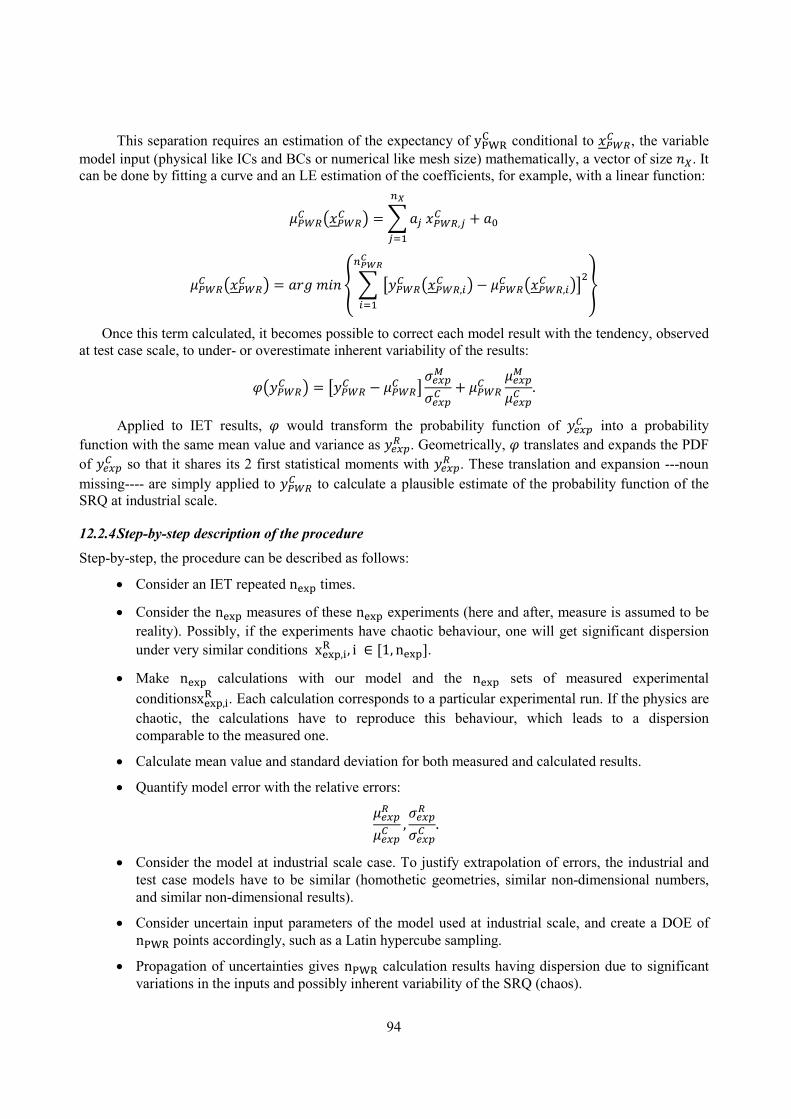
94

This separation requires an estimation of the expectancy of yPWRC conditional to 𝑥𝑥𝑃𝑃𝑃𝑃𝑛𝑛

𝐶𝐶 , the variable model input (physical like ICs and BCs or numerical like mesh size) mathematically, a vector of size 𝑛𝑛𝑋𝑋. It can be done by fitting a curve and an LE estimation of the coefficients, for example, with a linear function:

𝜇𝜇𝑃𝑃𝑃𝑃𝑛𝑛𝐶𝐶 𝑥𝑥𝑃𝑃𝑃𝑃𝑛𝑛

𝐶𝐶 = 𝑎𝑎𝑗𝑗 𝑥𝑥𝑃𝑃𝑃𝑃𝑛𝑛,𝑗𝑗𝐶𝐶 + 𝑎𝑎0

𝑛𝑛𝑋𝑋

𝑗𝑗=1

𝜇𝜇𝑃𝑃𝑃𝑃𝑛𝑛𝐶𝐶 𝑥𝑥𝑃𝑃𝑃𝑃𝑛𝑛

𝐶𝐶 = 𝑎𝑎𝑟𝑟𝑎𝑎 𝑚𝑚𝑚𝑚𝑛𝑛 𝑦𝑦𝑃𝑃𝑃𝑃𝑛𝑛𝐶𝐶 𝑥𝑥𝑃𝑃𝑃𝑃𝑛𝑛,𝑖𝑖

𝐶𝐶 − 𝜇𝜇𝑃𝑃𝑃𝑃𝑛𝑛𝐶𝐶 𝑥𝑥𝑃𝑃𝑃𝑃𝑛𝑛,𝑖𝑖

𝐶𝐶 2𝑛𝑛𝑃𝑃𝑃𝑃𝑃𝑃𝐶𝐶

𝑖𝑖=1

Once this term calculated, it becomes possible to correct each model result with the tendency, observed at test case scale, to under- or overestimate inherent variability of the results:

𝜑𝜑𝑦𝑦𝑃𝑃𝑃𝑃𝑛𝑛𝐶𝐶 = 𝑦𝑦𝑃𝑃𝑃𝑃𝑛𝑛

𝐶𝐶 − 𝜇𝜇𝑃𝑃𝑃𝑃𝑛𝑛𝐶𝐶

𝜎𝜎𝑚𝑚𝑒𝑒𝑖𝑖𝑀𝑀

𝜎𝜎𝑚𝑚𝑒𝑒𝑖𝑖𝐶𝐶 + 𝜇𝜇𝑃𝑃𝑃𝑃𝑛𝑛𝐶𝐶 𝜇𝜇𝑚𝑚𝑒𝑒𝑖𝑖𝑀𝑀

𝜇𝜇𝑚𝑚𝑒𝑒𝑖𝑖𝐶𝐶 .

Applied to IET results, 𝜑𝜑 would transform the probability function of 𝑦𝑦𝑚𝑚𝑒𝑒𝑖𝑖𝐶𝐶 into a probability function with the same mean value and variance as 𝑦𝑦𝑚𝑚𝑒𝑒𝑖𝑖𝑛𝑛 . Geometrically, 𝜑𝜑 translates and expands the PDF of 𝑦𝑦𝑚𝑚𝑒𝑒𝑖𝑖𝐶𝐶 so that it shares its 2 first statistical moments with 𝑦𝑦𝑚𝑚𝑒𝑒𝑖𝑖𝑛𝑛 . These translation and expansion ---noun missing---- are simply applied to 𝑦𝑦𝑃𝑃𝑃𝑃𝑛𝑛

𝐶𝐶 to calculate a plausible estimate of the probability function of the SRQ at industrial scale.

12.2.4 Step-by-step description of the procedure

Step-by-step, the procedure can be described as follows:

• Consider an IET repeated nexp times.

• Consider the nexp measures of these nexp experiments (here and after, measure is assumed to be reality). Possibly, if the experiments have chaotic behaviour, one will get significant dispersion under very similar conditions xexp,i

R , i ∈ [1, nexp].

• Make nexp calculations with our model and the nexp sets of measured experimental conditionsxexp,i

R . Each calculation corresponds to a particular experimental run. If the physics are chaotic, the calculations have to reproduce this behaviour, which leads to a dispersion comparable to the measured one.

• Calculate mean value and standard deviation for both measured and calculated results.

• Quantify model error with the relative errors:

𝜇𝜇𝑚𝑚𝑒𝑒𝑖𝑖𝑛𝑛

𝜇𝜇𝑚𝑚𝑒𝑒𝑖𝑖𝐶𝐶 ,𝜎𝜎𝑚𝑚𝑒𝑒𝑖𝑖𝑛𝑛

𝜎𝜎𝑚𝑚𝑒𝑒𝑖𝑖𝐶𝐶 .

• Consider the model at industrial scale case. To justify extrapolation of errors, the industrial and test case models have to be similar (homothetic geometries, similar non-dimensional numbers, and similar non-dimensional results).

• Consider uncertain input parameters of the model used at industrial scale, and create a DOE of nPWR points accordingly, such as a Latin hypercube sampling.

• Propagation of uncertainties gives nPWR calculation results having dispersion due to significant variations in the inputs and possibly inherent variability of the SRQ (chaos).

95

• Correct each set of results yPWRC xPWR,i

C , i ∈ 1, nPWRC with φ.

• Depending on the subjective confidence in the transposability of results from IET to the reality of interest, the use of the corrected propagation results is at the discretion of the engineer in charge.

The use of the corrected propagation results cannot be blunt. Consider a situation where the corrected calculation results lead to bigger margin factors than the uncorrected ones: A perfectly valid decision would be to transfer to the next link in the chain of calculations used for safety demonstration the non-corrected results from CFD in order to lead to a conservative evaluation of the possible values of the margins. On the other hand, if the corrected calculation results lead to lesser margin factors, a perfectly valid decision would be to transfer the corrected results with an arbitrarily enlarged correction to the next link in order to lead, again, to a conservative evaluation of the possible values of the margins. At this point, the engineer judgement is still mandatory.

96

12.2.5 Conclusions on the procedure

The corrected propagation results take the following into account:

• Model flaws observed at IET scale

• Variability of the SRQ for the reality of interest due to significant uncertainty on input parameter values

• Possible inherent variability of the SRQ due to chaotic behaviour

• Extra uncertainty on the SRQ due to non-convergence of statistic estimators (by non-parametric bootstrapping not presented here)

In the presentation, 𝑦𝑦 was implicitly considered to be a scalar, but when dealing with time series, the procedure can be repeated at each time step. The same can be done for a function of space at each discrete position. This flexibility allows the respect of the rule that the UQ procedure has to provide results that actually correspond to normal model outputs and not only some statistical quantities.

In the end, a by-product of the procedure is an estimate of the impact of each source of uncertainty on calculation results with chaos and uncertain input parameters separated out.

12.2.6 Characteristics of the procedure

This procedure uses both extrapolation of errors and propagation methods.

Propagation does not belong to the meta-model category, but a meta-model is used for extrapolation of errors.

It addresses uncertainty due to uncertain input parameters such as ICs and BCs.

It addresses model form uncertainty by taking into account biases on mean value and standard deviation between computations and reference data on IET.

It can address uncertainty due to numerics. Calculations with different meshes are possible; in propagation, categorical variables can be used).

IET data are used in this procedure. The default choice is to have a number of computations on the IET scale equal to the number of experiments. There is no specific requirement for the number of experiments, but the number of calculations and amount of reference data at IET scale impacts estimates of uncertainty due to non-convergence of statistical estimators.

The procedure does not specifically include the effects of geometric simplification, but they might be taken into account if in the model biases are the same at IET and industrial scale.

It believes that the IET used is close enough to the application to transpose the model biases from it to the case of interest.

SETs are not used in this procedure.

With default choice, the number of computations at reactor scale does not depend on the number of uncertain input parameters (e.g. Latin hypercube sampling, Monte Carlo type methods). Again, the number of calculations impacts estimates of uncertainty due to non-convergence of statistical estimators. The maturity of this procedure is currently low.

97

98

13. CRITICAL REVIEW OF SOME CFD UQ INVESTIGATIONS FOUND IN THE LITERATURE

Very few applications of uncertainty methods in CFD were found in the context of nuclear reactor thermalhydraulics. However, to give readers an idea of the current activity in this field, the little information found in published papers and presentations is summarised here.

13.1 On the accuracy quantification for CFD

The work presented by Moretti and D’Auria (2012) is an attempt to address the issue of quantifying the accuracy of CFD code results by suitable metrics while taking the multi-dimensional nature of the data into account. Nuclear reactor in-vessel flows featuring perturbations of coolant properties at the core inlet (e.g. during boron dilution transients and steam generator (SG) overcooling transients) are considered reference situations of interest. The authors observe that code-to-experiment comparisons relying on poor quantitative analysis, in which only a few averaged or extreme quantities are compared without fully exploiting the amount of information embedded in a CFD-grade data set and in CFD calculation results, may be inadequate as far as code qualification for NRS is concerned (Moretti and D’Auria, 2012). They then propose a method for the quantitative characterisation of both the measured and calculated time and space distribution of target quantities such as the coolant temperature and the boron concentration and of related discrepancies. The method uses the calculation of over 20 “accuracy quantifiers,” which are scalar parameters defined to capture different key/critical aspects of the variable distributions to which they are related. The following is a list of some of the parameters Moretti and D’Auria (2012) define as accuracy quantifiers:

• Perturbation appearance

• Overall maximum perturbation

• Core-averaged perturbation

• Accumulated perturbation

• Perturbation barycentre

• FLOMIX-type deviations [i.e., similar to those adopted in the framework of the FLOMIX-R European Project ]

• Spatial gradients

• Application of the 3D Fast Fourier Transform

In particular, some scalar parameters can be considered “mixing indicators” because they are directly affected by the amount of mixing the perturbed coolant experiences. Some examples of such mixing indicators are perturbation transit time through the core inlet; the maximum value of the perturbation over time and space; the maximum value of the core-averaged perturbation; the maximum and time-averaged values of the standard deviation of the spatial distribution, which is related to the spatial gradients of the distribution itself, which are, in turn, influenced by the mixing; and the maximum slope of the spatial distribution of the perturbation.

99

A preliminary assessment of the above approach is performed by applying it to the CFD code validation database available at the University of Pisa. Further assessment and improvement of the method by extending it to a wider validation database is recommended. Moreover, the definition of acceptance criteria for the accuracy quantifiers also needs to be addressed in future development.

The proposed method could be integrated into a UMAE-like framework for qualification and uncertainty evaluation.

13.2 An application of a solution verification for CFD

An article by Tanaka (2012) describes a complete application of so-called “solution verification”, i.e., the evaluation of the uncertainty of the code due to numerical error. It consists of the Richardson’s extrapolation, then GCI as defined by Roache and finally, the estimation of the standard deviation associated with the numerical error according to the recommendations of the ASME V&V 20-2009. The application case is the prediction of structural thermal fatigue caused by high cycle thermal mixing phenomena, a very important issue in design and safety of advanced sodium-cooled fast reactors such as the Japan sodium-cooled fast reactor (JSFR). The code used is MUGTHES.

In the first step, called verification, the method is applied to 5 simple cases of laminar flow and structure heat conduction problems. An “exact” value of each response, for example, the points of a velocity profile, is obtained by DNS, experiment or theory. An extrapolated value is estimated for each response by using RE. The local 𝐺𝐺𝐺𝐺𝐺𝐺𝑖𝑖 is derived from the extrapolated value with a safety factor equal to 1.25. Then an overall 𝐺𝐺𝐺𝐺𝐺𝐺 in the domain is calculated via the Root Mean Square (RMS) function using the

local 𝐺𝐺𝐺𝐺𝐺𝐺𝑖𝑖 for all responses: 𝐺𝐺𝐺𝐺𝐺𝐺 = 1𝑀𝑀∑ (𝐺𝐺𝐺𝐺𝐺𝐺𝑖𝑖)2𝑀𝑀𝑖𝑖=1 , 𝑀𝑀 being the number of responses. The standard

deviation coming from the numerical error is defined as 𝜎𝜎𝑒𝑒 = 𝐺𝐺𝐺𝐺𝐺𝐺 1.15⁄ , as recommended by ASME. Because exact solutions are known for these simple cases, the author adds an uncertainty factor based on the difference between the exact and extrapolated results defined as follows:

𝜀𝜀𝐶𝐶 = ∑ 1𝑀𝑀(𝜙𝜙𝑖𝑖)𝑚𝑚𝑒𝑒𝑣𝑣𝑒𝑒𝑡𝑡 − (𝜙𝜙𝑖𝑖)𝑚𝑚𝑒𝑒𝑡𝑡𝑟𝑟𝑣𝑣𝑖𝑖𝑚𝑚𝑣𝑣𝑣𝑣𝑡𝑡𝑚𝑚𝑚𝑚

2𝑀𝑀𝑖𝑖=1 . Finally the combined standard uncertainty is defined by

𝜎𝜎𝑆𝑆 = 𝜎𝜎𝐶𝐶2 + 𝜀𝜀𝐶𝐶2.

In the last part of the Moretti and D’Auria (2012) article, validation is performed by considering a practical fluid structure thermal interaction problem in a T-junction pipe system. This case is at a higher scale than the 5 simple ones, and LES is used to model turbulence. Uncertainty bands are estimated for velocities as well as fluid and structure temperatures. The experimental results are bounded by the error bars deduced from the application of the whole method.

100

13.3 Iaccarino’s vision of UQ

Iaccarino’s approach to UQ is quite analogous to the ideas already expressed in this document (Iaccarino, presentation made at Von Karman Institute). He divides the UQ problem into three steps (Figure 13.1):

Figure 13.1: Schematic of whole UQ process. Items in blue are not discussed in this report

1. Data assimilation: In this step, we must characterise the input uncertainties. That includes determining all sources of uncertainties, their nature (e.g. aleatoric and epistemic), and how they can be represented. This characterisation is essential for selecting the propagation method. No explicit method for determining the sources of uncertainties is mentioned, but the sources of uncertainty in CFD are well established. They include numerical errors (mesh resolution, advection schemes, solution of the linear systems, coupling algorithms, etc.), uncertain initial and boundary conditions (including variability of system geometry due to fabrication tolerance), uncertain physical properties (which are measured experimentally), and epistemic uncertainties in the turbulence models. After all sources of uncertainties have been determined, we must gather and analyse the available information about the input parameters in order to define how their uncertainties will be represented (e.g. interval, PDF, fuzzy). The main difficulties in data assimilation are uncovering and evaluating correlations of input parameters and building credible distributions based on sparse and/or contradictory evidence.

2. Propagation: After the sources of uncertainties have been identified and characterised, we can propagate them through the simulations. The selection of the propagation method depends on the nature of the uncertainty in the input parameters. For instance, when inputs are represented in terms of an interval, the propagation method can be probabilistic or non-probabilistic. For the non-probabilistic interpretation of

101

the input parameter, the interval represents the portion of the parameter-space in which the variable can exist. In this case, the input parameter is not considered random but as a deterministic variable without certainty of its value in the support interval. Iaccarino points out that this non-probabilistic interpretation of the input parameters is different than that of using a uniform PDF where all values are equally probable. For a non-probabilistic interval interpretation of the input parameter, the propagation method focusses on evaluating the response of the system at the extremes of each input interval. Thus, if we are interested in the output interval for temperature at a given location, we should evaluate the CFD simulations at the maximum and minimum values of each input parameter and then take the global maximum and minimum of the temperature measurements at that location. In Iaccarino’s vision, this type of analysis is equivalent to considering the worst case scenario. The problem with this approach is that to properly bound the response using the minimum and maximum of the random inputs, it must be monotonic in the multi-dimensional support interval, a condition that cannot be guaranteed a priori. This is illustrated in Figure

13.2, where the response of the system in the interval [ ]ba xx , is not monotonic. The danger of estimating

the interval for the response [ ]ba RR , when the maximum value for the response cannot be obtained by evaluating the response at the extremes of the support interval for the input parameter can be clearly observed. When the input random variables are represented by a PDF (e.g. Gaussian or uniform), the propagation step can be performed with conventional methods such as Monte Carlo, PCE, or response surface + Monte Carlo.

Figure 13.2: Schematic of the uncertainty propagation in a non-liner system

3. Certification: In this step, the uncertainty bands are determined, including the acceptance criteria for the simulations. For probabilistic propagation methods, uncertainty bands are usually expressed in terms of an expected value and a multiple of the standard deviation ( )σnx ± .

As mentioned in step 1, the characterisation of uncertainties is vital for selecting the propagation method. The three primary ways to characterise the input uncertainties are by using intervals, PDFs, and membership function (fuzzy numbers). These three methods of characterizing uncertainty are schematically depicted in Figure 13.3. The output uncertainty would then be a combination of these three types of individual uncertainties.

Input uncertainties can be classified into two main groups: aleatory (stochastic) and epistemic. Iaccarino (year) mentions that epistemic uncertainties are NOT naturally treated in a probability framework.

102

Figure 13.3: Schematic representation of input uncertainty

13.4 Methods for epistemic uncertainties

• Second order probabilities: PDFs are not certain (see Figure 13.4). No details are provided on how to propagate these uncertain PDFs.

Figure 13.4: A probability density function for uncertain input

• Intervals: Input uncertainties are characterised by an interval [ ]maxmin , xx . The output uncertainty interval is obtained by taking the global maximum and the global minimum of the response evaluated at the extremes of each input interval. For only one input parameter, this is equivalent to ( ) ( ) ( ) ( ) [ ]maxminmaxmin ,max,,min xRxRxRxR . Another way to treat intervals is to use Taylor models, where the response is expressed in term of a polynomial of degree n + an interval remainder nI , that is nn IPR += .

• Evidence theory: Basically this method is expert judgement, where the concept of belief is introduced. From a personal point of view, I think that in this case we can use a Bayesian approach to construct a PDF for the input random parameters based on expert judgement and quantitative information available. In a Bayesian probability framework, a PDF represents the degree of belief in a certain proposition. Once there is a PDF, either frequentist or Bayesian, any standard probabilistic propagation method can be used. This simplifies the calculation of response uncertainty, but it could lead to a large increase in the computational cost. For instance, having two inputs—one characterised by an interval and the other by a PDF—, we would need to sample the response only twice for the first one and several times for the second one. Nonetheless, the use of intervals should be restricted to systems that are clearly monotonic. For CFD simulations, monotonic behaviour of the responses cannot be guaranteed a priori for the input parameters. The use of intervals in UQ for CFD could substantially decrease the computational cost but at the expense of having less reliable output uncertainties. In addition, intervals cannot be used in a formal sensibility analysis such as Sobol’s indices.

103

In summary, Iaccarino’s general approach to UQ (data assimilation, propagation, certification) is similar to what we have already presented in this document. The data assimilation step is the most relevant one in the whole UQ methodology. Although the propagation step can be very computationally demanding, without a the proper characterisation of the inputs, the output uncertainties become less reliable. Hence, we must make an effort to establish a comprehensive methodology for determining the input uncertainties. The mathematical details of the propagation methods are straightforward and can be found elsewhere.

13.5 An uncertainty analysis of coupled system-CFD codes

Geffray et al.’s 2015 paper describes an uncertainty and sensitivity analysis which was performed for a coupled ATHLET-ANSYS-CFX simulation of a TALL-3D experiment. The TALL-3D thermal-hydraulic loop is an integral, well instrumented, 7 m tall, lead-bismuth eutectic (LBE) experimental facility, operated by the Royal Institute of Technology in Sweden (KTH). It is equipped with a 3D test section. In the experiment T01, the main circulation pump is stopped, simulating the trip of a primary pump while both heaters remain on. This leads to a transition from forced circulation steady-state to natural circulation steady-state with local 3D phenomena like LBE mixing, stratification, and flow reversal in the 3D test section leg.

In the context of the European project Thermal Hydraulics of Innovative Nuclear Systems (THINS) , the German Gesellschaft für Anlagen- und Reaktorsicherheit mbH (GRS) has extended the capability of the coupling between the CFD code ANSYS-CFX and the in-house system analysis code ATHLET to model LBE flows. In the simulation of the TALL-3D experiment T01, the test section pool with its inlet and outlet pipes were modelled using ANSYS-CFX, while the rest of the facility is represented with ATHLET.

At the Technische Universität München (TUM, Germany), a computational framework was developed to propagate modelling uncertainty through the coupled ATHLET-ANSYS CFD codes. This method was applied to the coupled simulation performed for the TALL-3D experiments. All parameters used to model the complex TALL-3D experiment, including initial and boundary conditions as well as physical models, were considered sources of uncertainty. Using a MatLab code developed in the context of the project, a sensitivity analysis determined the most influential input uncertain parameters and an uncertainty analysis the range of variability of output variables due to the uncertainty of input parameters Two-sided 95%/95% tolerance limits were calculated according to Hofer (1999). This approach has a low computational cost with only 93 runs in the present case and is non-parametric, so no assumptions need to be made regarding the underlying PDF of the output.

The uncertainty and sensitivity analyses show good agreement between the model and the experimental results, even though the modelling of the physical phenomena is challenging. The results of the sensitivity analysis allow further characterisation of the model behaviour and identification of the most influential model input parameters. The results reported here are highly consistent. Parameters such as the power of the heaters and pressure losses at the electric permanent magnet-pump need be determined more accurately so that the related uncertainty can be reduced thus, allowing an increase in the model prediction accuracy.

104

14. SYNTHESIS OF THE REVIEW

The various methods covered in this review and their characteristics are synthesised in Table 14.1.

The methods described vary in their purposes and other aspects. Some are propagation methods; others are extrapolation methods; still other could be combinations of both. In principle, they may address all sources of uncertainties but in different ways depending on the method.

Some propagation methods use meta-models in view of limiting the number of simulations. Due to CPU cost, the total number of required CFD simulations may be an important criterion in the choice of a method.

An evaluation of the degree of maturity of the methods can also be helpful. Four levels of maturity are considered:

• High: The methodology is well established; it has already been applied to simple test cases and to reactor issues. The results were satisfactory.

• Medium: The methodology is established but may be improved; it was applied to simple test cases and to reactor issues. The results are promising but not fully satisfactory.

• Low: The methodology is established but needs improvement; it was applied to simple test cases only.

• Very Low: The methodology is established but requires further elaboration; it has not yet been applied even to simple test cases.

105

Basic methodology Methods Used Addressing the sources of uncertainty Use of SETs Use of IETs

Nb of reactor

calc.

Degree of maturity

IC &

BC

Para

met

ers o

f ph

ysic

al m

odel

s

Non

-mod

elle

d pr

oces

ses

Mod

el o

ptio

ns

Dis

cret

isat

ion

itera

tion

roun

d-of

f er

rors

Num

eric

al o

ptio

ns

Geo

met

ric

sim

plifi

catio

ns

Scal

ing

dist

ortio

ns

Num

ber

Num

ber

Propagation methods

Monte Carlo random

sampling OK OK No OK OK OK OK OK Can

use Many No 100 or more Low

Use of meta-models PCE Only a few of them: N Can

use Many No !!)!(

LNLN +

Low;

High for propagation

Deterministic sampling DS Only a few of them Can

use Many No Low

Extrapolation methods

Extended UMAE

Not

fully All of them are collectively accounted for, though

not explicitly and individually addressed. Must use Many Must

use Many 1 Very low

Based on ASME

In principle, may address all.

May depend on how ASME method is extended. No Must

use 1 or a few 1 Very low

Combined propagation & extrapolation

method

Use of meta- models or not

A few by propagation;

others by extrapolation Can use Many Must

use A few Several Low

Table 14.1: Characteristics of the various methods covered in this review

NEA/CSNI/R(2016)4

106

In the course of this review, the following observations were made:

• Propagation methods may take all input uncertainties – except those due to non-modelled physical processes – but require many reactor calculations when using a Monte Carlo approach.

• DS may optimise the number of calculations necessary.

• When using a meta-model, propagation methods require fewer reactor calculations but may not address all sources of uncertainties.

• Extrapolation methods require significantly fewer reactor calculations but need preliminary SET and/or IET calculations. To some extent, they may take the uncertainty due to non-modelled processes into account. They do not rigorously address uncertainty due to reactor initial and boundary conditions (IC-BC) or material properties since they can only extrapolate those of IETs, which are better known than those for reactors.

• When using IET calculations, extrapolation methods have a better chance of including the effects of non-modelled phenomena than do propagation methods.

• A combination of extrapolation and propagation seems possible using meta-models. It might address some sources of uncertainty created by propagation while some other uncertainties are added a posteriori by extrapolation from IET validation.

• The degree of maturity of these methods is either low or very low.

NEA/CSNI/R(2016)4

107

15. CONCLUSIONS AND RECOMMENDATIONS

The use of single-phase CFD for reactor safety requires rigorous adherence to a general methodology that includes a PIRT analysis, a scaling analysis, the scaling of some experiments, the selection of an appropriate CFD tool and of appropriate physical and numerical options, the building of an appropriate nodalisation, the application of existing BPG in the previous two steps, a comprehensive V&V programme for the situation of interest, and the application of a mature UQ method. Previous activities within WGAMA have elaborated BPGs and identified assessment matrices for selected safety issues, but the lack of a consolidated uncertainty method is the main limitation for CFD application to safety demonstration.

A review of existing work in this field was made, but only very limited information was found regarding CFD UQ applied to nuclear reactor safety analysis. The main reactor issues for which CFD UQ methods are expected to be applicable in the short and medium term are mixing problems (temperature, boron concentration, H2 concentration, etc.) with or without density effects.

The two types of methods developed and used for UQ of system codes may be extended to CFD with some adaptations, specifically:

• The methods based on the propagation of input parameter uncertainty

• The methods based on the extrapolation of accuracy

The adaptation of the methods is still in progress, and from the first few applications, the feedback is rather limited. In spite of that, here are some preliminary observations and conclusions.

• The various sources of code prediction uncertainty include initial and boundary conditions, physical properties, parameters of the physical models, non-modelled physical processes, numerical models, numerical solution errors, simplifications of geometry, possible chaotic behaviour, and extrapolation beyond the validated domain.

• The propagation method with Monte Carlo sampling is applicable to CFD even with a large number of input uncertain parameters, but it may lead to prohibitive CPU cost.

• The use of DS rather than random sampling may be a cheaper alternative for propagation methods

• The use of meta-models may be a somewhat cheaper alternative for propagation methods when the number of input uncertain parameters is low. When used at first order, it is close to the DS method in terms of the required number of calculations.

• The determination of uncertainty due to physical models is not straightforward for propagation methods. For example, uncertainty on parameters of turbulence models may depend strongly on the type of flow configuration.

• Extrapolation methods have the advantage of taking benefit from IETs, which are often designed to study the safety issue of interest. They require less CPU cost than Monte Carlo propagation methods. However, preliminary work on the calculation of many SETs and IETs is necessary. Moreover, it has yet to be proved that a pure extrapolation method like UMAE can be adapted or extended to CFD.

• The uncertainty due to numerics compared to other sources of uncertainty is relatively more important than for system codes and requires special attention. Methods for numerical error evaluation exist, but they may fail or be difficult to use in practical applications.

NEA/CSNI/R(2016)4

108

• The validation of the CFD tool on scaled IETs relative to a situation of interest seems to be mandatory in the V&V process and in both V&V and UQ steps.

• A combination of propagation and extrapolation techniques may be a reasonable compromise in order to limit the number of calculations and the CPU cost.

• The CPU cost is still the main hindrance to CFD application, but the continuing improvements in computer efficiency are progressively eroding this obstacle.

The maturity levels of all the reviewed methods are medium to very low. Some methods need extensions or adaptations for CFD as well as extensive testing, and all need to be benchmarked. Benchmarking is necessary. Consequently, the main recommendations are as follows:

• An effort should be devoted to determine uncertainty due to physical models for propagation methods. Methods should be tested following what has been done in the PREMIUM (www.oecd-nea.org) benchmark for system codes.

• Further R&D work on numerical error estimation is recommended.

• A first benchmark needs to be done and should be based on simple tests and require minimum CPU costs in order to test all types of methods including the propagation methods with statistical sampling. It should be as close as possible to the mixing with density effects encountered in some reactor safety issues. The GEMIX benchmark meets the requirements.

• A second benchmark should be closer to real application and should use one of the CETs (or demonstration) designed to investigate reactor issues.

Although the CFD UQ is still immature, application of some existing methods – if properly extended and tested – seems achievable.

The application of single-phase CFD in a first step for safety demonstration does not create insurmountable difficulties, and in the short or medium term, this new technology could reach a degree of maturity comparable to that of system codes, at least for a few applications. The application of BPGs, comprehensive assessments relative to the specific applications, and a consolidated UQ method are the main requirements. A high priority should be put on progress on the last item.

NEA/CSNI/R(2016)4

109

16. REFERENCES

Accident analysis for NPPs, Safety Reports Series No.23, IAEA, 2002.

Ambrosini W., Bovalini R., D’Auria F., “Evaluation of Accuracy of Thermal-hydraulic Codes Calculations”, Energia Nucleare, 7, No. 2, 1990.

G. Anderson, “Error propagation by the Monte Carlo method in geochemical calculations”, Geochim. Cosmochim. Ac., vol. 40, pp. 1533-1538, 1976.

Angrisani & al., “Unscented transform: A powerful tool for measurement uncertainty evaluation”. IEEE Transactions on instrumentation and measurement 2006, Vol. 55, pp. 737-743.

ASME Report V&V 20-2009, Standard for Verification and Validation in Computational Fluid Dynamics and Heat Transfer, November 2009

F. D’Auria, E. Chojnacki, H. Glaeser, C. Lage, T. Wickett, Overview of Uncertainty issues and Methodologies”, Invited at OECD/CSNI Seminar on Best Estimate Methods in Thermal Hydraulic Safety Analyses, Ankara (Tr) June 29- July 1, 1998.

D’Auria, F., Galassi G.M. 2010. Scaling in nuclear reactor system thermal-hydraulics, Nuclear Engineering and Design, doi:10.1016/j.nucengdes.2010.06.010

D'Auria, F., Debrecin, N., Galassi, G.M. 1995, Outline of the Uncertainty Methodology based on Accuracy Extrapolation (UMAE). Nuclear Technology, 109, 1, 21-38.

D’Auria, F., Giannotti, W. 2000, Development of Code with capability of Internal Assessment of Uncertainty, Nuclear Technology, 131, 1, 159-196.

D’Auria F., Giannotti W., Development of Code with capability of Internal Assessment of Uncertainty, J. Nuclear Technology, Vol 131, No. 1, pages 159-196 – Aug. 2000.

A. Badillo, R. Kapulla, B. Niceno, “Uncertainty Quantification in CFD Simulations of Isokinetic Turbulent Mixing Layers”, Proceedings of the NURETH-15 Congress, paper-559, Pisa, Italy 2013.

D. Bestion, H. Anglart, B.L. Smith, J. Royen, M. Andreani, J.H. Mahaffy, F. Kasahara, E. Komen, P. Mühlbauer, T. Morii, M. Scheuerer, E. Laurien, T. Watanabe, A. Dehbi, Extension of CFD Codes to Two-Phase Flow Safety Problems, NEA/SEN/SIN/AMA(2006)2

D. Bestion, H. Anglart, J. Mahaffy, D. Lucas, C.H. Song, M. Scheuerer, G. Zigh, M. Andreani, F. Kasahara, M. Heitsch, E. Komen, F. Moretti, T. Morii, P. Mühlbauer, B.L. Smith, T. Watanabe, Extension of CFD Codes to Two-Phase Flow Safety Problems, NEA-CSNI-R(2010)2

X.Chen, B. Ng, Y. Sun, C. Tong, “A flexible uncertainty quantification method for linearly coupled multi-physics systems” Journal of Computational Physics, Vol 248 pp 383-401 (2013)

A. de Crécy, P. Bazin, Quantification of the uncertainties of the physical models of CATHARE 2, M&C 2001, Salt lake City, Utah, USA, September 2001, ANS Winter Meeting, Washington, DC, USA, Nov. 14-18, 2004

A. de Crécy, P. Bazin (Editors), H. Glaeser, T. Skorek, J. Joucla, P. Probst, B. Chung, D.-Y. Oh, M. Kynck, R. Pernica, J. Macek, R. Meca, R. Macian, F. D’Auria, A. Petruzzi, M. Perez, F. Reventos, K. Fujioka, Bemuse Phase III Report, Uncertainty and Sensitivity Analysis of the LOFT L2-5 Test, OECD/CSNI Report NEA/CSNI/R(2007)4, October 2007

NEA/CSNI/R(2016)4

110

L. Eça, M. Hoekstra, An evaluation of verification procedures for CFD applications, 24th Symposium on Naval Hydrodynamics, Fukuoka, Japan, 8-13 July 2002.

E.C. Eggertson, R. Kapulla, J. Fokken and H.M. Prasser, “Turbulent Mixing and its effects on thermal fatigue in nuclear reactors”, Proceedings of World Academy of Science, Engineering and Technology, Volume 76, pp. 206-213, 2011.

L. Fagiano and M. Khammash, “Simulation of stochastic systems via polynomial chaos expansions and convex optimization”, Phys. Rev. E, vol. 86, 036702, 2012.

J. Fokken, R. Kapulla, G. Galgani, O. Schieb, K. Pawa and H.M. Prasser, “LIF-Measurements and self-similarity considerations in a stably stratified isokinetic turbulent mixing layer”, Proceedings of 18. GALA-Fachtagung: Lasermethoden in der Strömungsmesstechnik, Cottbus, Germany, September, 2010.

C. Geffray, R. Macián-Juan, A. Papukchiev, D. Grischenko, P. Kudinov, UNCERTAINTY AND SENSITIVITY ANALYSIS OF THE TALL-3D EXPERIMENT USING THERMAL-HYDRAULIC COUPLED CODES, paper 15327 in the proceedings of ICAPP 2015, Nice, France (2015)

E. HOFER, “Sensitivity analysis in the context of uncertainty analysis for computationally intensive models”, Computer Physics Communications, 117, Computer Physics Communications, 117, Issues 1–2, 1 03/1999, 21-34.

Hessling JP. , “Deterministic Sampling for propagating model covariance”, SIAM/ASA Journal on Uncertainty Quantification 2013, Vol. 1, pp297-318.

S. Hosder, R. Walters and R. Perez, “A non-intrusive polynomial chaos method for uncertainty propagation in CFD simulations”, Proceedings of the 44th AIAA Aerospace Science, Vol 14, pp 1064-10667, Reno, USA, 2006

ISO GUM, Guide to the Expression of Uncertainty in Measurement, Tech. Rep., International Organization for Standardization, Geneva, Switzerland (1995).JCGM 100:2008. Evaluation of measurement data - Guide to the expression of uncertainty in measurement, Joint Committee for Guides in Metrology

J. NED, Special Issue, 1990, Vol 119, 1, devoted to CSAU.

S. Julier, J. Uhlmann, Unscented filtering and nonlinear estimation, in: Proceedings IEEE, 2004, Vol. 92, pp. 401-422.

O.M. Knio and O.P. Le Maître, “Uncertainty Propagation in CFD Using Polynomial Chaos Decomposition”, Fluid Dynamics Research, vol. 38, pp. 616–640, 2006.

A.K. Kuczaj, E.M.J. Komen, M.S. Loginov, “Large-Eddy Simulation study of turbulent mixing in a T-junction”, Nuclear Engineering and Design, vol. 240(9), pp. 2116-2122, 2010.

S. Kuhn, O. Braillard, B. Ničeno, H.-M. Prasser, “Computational study of conjugate heat transfer in T-junctions”, Nuclear Engineering and Design, vol. 240(6), pp. 1548-1557, 2010.

D. Lucor, J. Meyers and P. Sagaut, “Sensitivity analysis of large-eddy simulations to subgrid-scale-model parametric uncertainty using polynomial chaos”, J. Fluid. Mech. Vol 585, pp. 255-279, 2007.

Mahaffy, J. (ed.) Best practice guidelines for the use of CFD in nuclear reactor safety applications, OECD, Nuclear Energy Agency, Technical Report, NEA/CSNI/R(2007)5, April 2007.

P. Manneville, Instabilities, Chaos and Turbulence, Imperial College Press, 2010.

M. Meldi, M. V. Salvetti, and P. Sagaut, “Quantification of errors in large-eddy simulations of a spatially evolving mixing layer using polynomial chaos”, Phys. Fluids, vol. 24, 035101, 2012.

K.-J. Metzner and U. Wilke, “European THERFAT project—thermal fatigue evaluation of piping system T-connections”, Nuclear Engineering and Design, vol. 235(2-4), pp. 473-484, 2006.

NEA/CSNI/R(2016)4

111

Moretti, F., D’Auria, F., Accuracy quantification metrics for CFD simulation of in-vessel flows. Nucl. Eng. Des. 279 (2014), pp. 200-209.

J.L.Muñoz-Cobo, A.Escrivá, R.M.Sanz, F.Pelayo, J.Melara, D.Mollá “CSAU methodology and results for an ATWS event using information theory methods”, Proceedings of the NURETH-15 Congress, Pisa, Italy 2013

H. Najm, “Uncertainty Quantification and Polynomial Chaos Techniques in Computational Fluid Dynamics”, Annu. Rev. Fluid. Mech. Vol 41, pp. 35-52, 2009.

OECD/CSNI, 1998. Report of the Uncertainty Methods Study for advanced best estimate thermal-hydraulic code applications. Vol I & II. OECD/CSNI Report NEA/CSNI/R(97)35, Paris (F)

A. Olsson, G. Sandberg, O. Dahlblom, “On Latin hypercube sampling for structural reliability analysis”, Struct. Safety, vol. 25, pp. 47-68, 2003.

W.L. Oberkampf & C.J. Roy, Verification and Validation in Scientific Computing, Cambridge University Press, 2010.

L. Parussini, V.Pediroda, C. Poloni, “Prediction of geometric uncertainty effects on fluid dynamics by polynomial chaos and fictitious domain method”, Computer &Fluids Vol 39, pp 137-151 (2010)

Petruzzi, A., D’Auria, F. 2008. Approaches, Relevant Topics, and Internal Method for Uncertainty Evaluation in Predictions of Thermal-Hydraulic System Codes, J. Science and Technology of Nuclear Installations, Vol 2008, Art. ID 325071

Petruzzi, A., D’Auria, F. (Editors), De Crécy, A., Bazin, P., Borisov, S., Skorek, T., Glaeser, H., Benoit, J.P., Chojnacki, E., Fujioka, K., Inoue S., Chung, B.D., Trosztel, I., Toth, I., Oh, D.Y., Pernica, R., Kyncl, M., Macek, J., Macian, R., Tanker, E., Soyer, A.E., Ozdere, O., Perez, M., Reventos, F. 2006, BEMUSE Programme. Phase 2 report <Re-Analysis of the ISP-13 Exercise, post-test analysis of the LOFT L2-5 experiment. OECD/CSNI Report NEA/CSNI/R(2006)2, 1-625.

Post-BEMUSE Reflood Model Input Uncertainty Methods (PREMIUM) Benchmark Phase II: Identification of Influential Parameters, Nuclear Safety NEA/CSNI/R(2014)14, February 2015, www.oecd-nea.org

P. Prempranneerach, F.S. Hover, M.S. Triantafyllou, G.E. Karniadakis, “Uncertainty quantification in simulations of power systems: Multi-element polynomial chaos methods”, Reliability Engineering and System Safety, Vol 95 pp 632-646, (2010)

Prošek, A., F. D'Auria, and B. Mavko, Review of Quantitative Accuracy Assessments with FFTBM, Nucl. Eng. and Des., Vol. 217, Is. 1-2, 2002.

L. F. Richardson, The approximate arithmetical solution by finite differences of physical problems involving differential equations, with an application to the stresses in a monsonry dam, Transactions of the Royal Society of London, Ser. A, Vol. 210, pp 307-357, 1910.

R. Rintamaa, I. Aho-Mantila, “Plant life management and modernisation: Research challenges in the EU”, Nuclear Engineering and Design, vol. 241(9), pp. 3389-3394, 2011.

Roache, P.J., “ Quantification of uncertainty in computational fluid dynamics” Annu. Rev. Fluid. Mech. 1997. 29:123–160.

P. J. Roache, Verification and validation in computational science and engineering, Hermosa publishing, Albuquerque, 1998.

F.Simon, P.Guillen, P.Sagaut, D.Lucor, “A GPC approach to uncertain transonic aerodynamics”, Comp. Method Applied Mech. Eng. Vol 199, pp 1091-109 (2010)

B.L. Smith, U. Bieder, E. Graffard, M. Heitsch, M. Henriksson,T. Höhne, E. Komen, J. Mahaffy, F. Moretti, T. Morii, P. Mühlbauer, U. Rohde, M. Scheuerer, C.-H. Song, G. Zigh, M. Andreani, D. Bestion,

NEA/CSNI/R(2016)4

112

F. Ducros, M. Houkema, D. Lucas, F. Menter, T. Watanabe, “Assessment of Computational Fluid Dynamics (CFD) for Nuclear Reactor Safety Problems”, OECD Nuclear Energy Agency, Technical Report, NEA/CSNI/R(2007)13, Jan. 2008

B.L. Smith, J.H. Mahaffy, K. Angele, J. Westin, “Report of the OECD/NEA-Vattenfal T-junction Benchmark exercise”, NEA/CSNI Report, 2011.

F. Stern & al, DOI: 10.1115/1.1412235 - ASME - Journal of Fluids Engineering – December 2001, Vol. 123 (pages 793 à 802) - “Comprehensive Approach to V&V of CFD Part1: Methodology” –.

F. Stern & al, DOI: 10.1115/1.1412236 - ASME - Journal of Fluids Engineering – December 2001, Vol. 123 (pages 803 à 810) - “Comprehensive Approach to V&V of CFD Part 2: Application for Rans Simulation of a Cargo/Container Ship” –.

M. Tanaka, Uncertainty Quantification Scheme in V&V of Fluid-Structure Thermal Interaction Code for Thermal Fatigue Issue in a Sodium cooled Fast Reactor, CFD4NRS-4, 2012

Tao Xing, Frederik Stern, Factors of Safety for Richardson Extrapolation, Journal of Fluids Engineering, June 2010, Vol. 132, p. 061403.

VV-20 Committee “Standard for verification and validation in CFD and Heat Transfer” ASME VV-20-2009.

M.M.R.Williams, “Polynomial chaos function and stochastic differential equations” Annals of Nuclear Energy Vol 33 pp 774-785, 2006

D. Xiu, G.E. Karniadakis, “Modeling uncertainty in flow simulations via generated polynomial chaos”, Journal of Computational Physics vol 187, pp 137-167 (2003)

G. E. Wilson, B. E. Boyack “The role of the PIRT process in experiments, code development and code applications associated with reactor safety analysis”, Nuclear Engineering and Design, 186, 23–37 (1998).

Wulff, W. 1996, Scaling of thermo-hydraulic systems, Nuclear Engineering & Design, 163, 359-395.

Zuber, N., 1991. Appendix D: a hierarchical, two-tiered scaling analysis, an integrated structure and scaling methodology for severe accident technical issue resolution. US Nuclear Regulatory Commission, Washington, DC 20555, NUREG/ CR-5809, November 1991

N. Zuber, G. E. Wilson, M. Ishii, W. Wulff, B. E. Boyack, A. E. Dukler, P. Griffith, J. M. Healzer, R. E. Henry, J. R. Lehner, S. Levy, F. J. Moody, M. Pilch, B. R. Seghal, B. W. Spencer, T. G. Theofanous, J. Valente “An integrated structure and scaling methodology for severe accident technical issue resolution: development of methodology”, Nuclear Engineering and Design, 186, 1–21 (1998).

Zuber, N., Wulff, W., Rohatgi, U.S., Catton, I. 2005. Application of Fractional Scaling Analysis (FSA) to Loss of Coolant Accidents (LOCA), Part 1: Methodology Development, Int. Top. Meet. on Nuclear Reactor Thermal Hydraulics (NURETH-11), Avignon (F).

NEA/CSNI/R(2016)4

113

17. NOMENCLATURE

Accuracy (qualitative and quantitative)

The accuracy of a simulation is a measure of the differences between the code predictions and the actual transient performance of a real facility or reactor. Qualitative accuracy is a non-numerical characterisation of the extent to which the code results reproduce the general trends, patterns, and phenomenological features that analysts, through their expert judgement, recognise in the experimental data. It is often defined by expressions like “fairly good agreement” and “unacceptable error”. Quantitative accuracy is defined by appropriate metrics that measure the discrepancies between code results and experimental data, such as mean error, bias, and standard deviation. Acceptance criteria may be defined to decide whether the achieved (accuracy – qualitative or quantitative – is satisfactory for the intended purpose.

Bias of calculation result

A bias is a measure of a systematic difference between an actual or true value and a predicted or measured value. Bias is the tendency of a model to systematically over-predict or under-predict data that are representative of an assigned phenomenon.

Code assessment

Code assessment is the process of verification and validation (V&V) that proves the capability of the physical models and of the numerical scheme of a code to simulate with sufficient accuracy and confidence the physical behaviours in a given domain of application.

Code qualification

Code qualification is the set of procedures used to prove that a code is able to do what it is designed for and that it meets all the associated requirements. Code qualification includes QA, V&V, and full documentation.

Confidence level

In the general context of confidence intervals probability that sample will contain the true parameter value.

In the context of statistical tolerance limits: probability β that the limits to be computed will cover the specified proportion α of the population (probability content α).

The confidence level is specified to account for a possible sampling error due to limited sample size, e.g. a limited number of calculations, from which the statements are obtained.

Confidence in validation

In statistics, “the confidence level” refers to the likelihood that the true parameter value lies within the range specified by the confidence interval. The confidence level is usually expressed as a percentage. Thus a 95% confidence level implies that the probability that the true parameter value lies within the confidence interval is

NEA/CSNI/R(2016)4

114

0.95. Here the confidence level implies the probability 0.95. In the area of V&V for system thermal-hydraulic codes, the confidence in validation indicates the level of satisfaction, on the results of the validation process by an observer. Therefore, the confidence in validation should be based on the quantitative evaluation of accuracy where proper acceptance criteria for the calculations (i.e., comparison between measured and predicted values) are fixed and met.

Closure relations

After averaging local instantaneous fluid balance equations, many terms in the resulting equations are new unknowns or contain new unknowns. At this point, the number of unknowns is greater than the number of equations, and the system of equations is not closed. In particular, averaged equations exhibit terms for transfers of mass, momentum, and energy at the walls and at the interfaces in two-phase or multi-fluid flow conditions. Constitutive relations are mathematical expressions for these phase-transfer terms as functions of the selected averaged principal variables. These are part of closure relations. Other relations are also necessary to express the average of nonlinear terms as functions of averaged main variables. The terminology “closure relations” derives from considering that they are necessary in order to close the system of equations. Some closure relations are simplifying assumptions such as <ρ(P,T)> = ρ(<P>, <T>). The closure relations typically encountered in the CFD are

• equations of state, i.e., relationships between averaged thermodynamic state quantities, e.g. = (p,T);

• relations that express the average of nonlinear terms as functions of averaged main variables such as those required in RANS and LES contexts to deal with the terms arising from time averaging and space filtering of the advection term of the Navier-Stokes equations, and

• constitutive relations needed to express, by ad hoc models, the transfers of mass, momentum, and energy at the walls and at the interfaces in two-phase or multi-fluid flow conditions or due to turbulence that arises from the averaging of local instantaneous fluid balance equations.

Combined effect test (CET)

A combined effect test (CET) is an experimental test performed in a test facility intended to simulate the behaviour of a complex system with multiple effects combined as in a reactor. Interactions could occur between various flows and heat transfer processes occurring in various system components such as an IET. The difference between a CET and an IET is that a CET does not necessarily include the whole cooling circuit. However, CET and IET terms are both used for some test facilities such as ROCOM.

Constitutive equations (see also closure relations)

Averaged fluid balance equations exhibit terms for transfers of mass, momentum, and energy at the walls and at the interfaces. Constitutive relations are expressions for these transfers as functions of principal variables. These are a subset of closure relations since they are necessary to close the system of equations.

Computational fluid dynamics (CFD)

The term “computational fluid dynamics” is very commonly used but is not well defined. Usually it refers to simulation tools that solve 3D fluid dynamics equations. This includes the RANS and LES approaches as well as the DNS, although practically inapplicable to cases of interest. It is not clear if CFD includes both porous medium approaches and open medium approaches, or just the latter. Therefore, it is recommended to specify porous-CFD and keep CFD for open medium approaches. Additionally, it is not clear if the term encompasses only single-phase and multi-phase CFD. The term computational multi-fluid dynamics (CMFD) was introduced

NEA/CSNI/R(2016)4

115

by Yadigaroglu to avoid confusion. The term CMFD is known in the nuclear thermal-hydraulic community but not in other domains.

Demonstration test

A demonstration test is a calculation test belonging to the verification of a code. Such a test is intended to assess whether the code is able to simulate at least qualitatively, without failure the behaviour of a complex system with all interactions between various flows and heat transfers processes occurring in various system components.

Direct numerical simulation (DNS)

Direct numerical simulation is a sort of “pure” CFD, in which the Navier-Stokes equations are numerically solved without applying any prior averaging or filtering techniques to treat the turbulence fluctuations. Hence, if the time and space discretisation is “sufficiently fine” (i.e., below the Kolmogorov scales), then the turbulence fluctuations can be resolved over their entire spectrum (i.e., at all space and time scales). Such discretisation requirements, even for relatively simple problems, usually lead to prohibitive computational costs.

Integral effect test (IET)

An integral effect test (IET) is an experimental test performed in an integral test facility (ITF) and is intended to simulate the behaviour of a complex system with all interactions between various flows and heat transfers processes occurring in various system components. An IET relative to reactor-accident thermal hydraulics may include the whole cooling circuit and simulates the accidental scenario through initial and boundary conditions.

Separate effect test or single effect test (SET)

Separate effect tests (SETs) are experimental tests intended to investigate a single physical process, either in the absence of other processes and/or in conditions which allow the effects of the process of interest to be measured. A SET may be used to validate a constitutive relation independently from the others.

Integral test facility (ITF)

An integral test facility (ITF) consists of an experimental loop designed according to a proper set of scaling laws and intended to simulate an entire nuclear power plant. It includes all the main components and geometrical zones of a nuclear power plant. Phenomena measured in an ITF are expected to be as similar as possible to those expected in the reference plant. The design of an ITF is usually based on a reference plant that has already been built or designed.

Large Eddy simulation (LES)

A large eddy simulation is space-filtered Navier-Stokes equations applied to a turbulent viscosity model in CFD tools.

Mesh (or meshing)

A mesh (or grid) is the ensemble of fundamental 3D polyhedral cells (tetrahedral, pyramids, hexahedra, and so forth) – along with the vertices, or nodes, and faces that define them – into which the computational domain of a CFD simulation is divided to allow the solution of the discretised balance equations. If a finite-volume solution method is used, as it is in most CFD codes, then the mesh defines the “control volumes” over which the equations are integrated. Depending on the specific code implementation, the control volumes either coincide with the above mentioned cells or they are polyhedral built around each node.

NEA/CSNI/R(2016)4

116

Mesh convergence

Mesh convergence is the process in which the mesh size of a nodalisation is decreased to the point at which the solution does not change anymore. When the numerical scheme is consistent and convergent, convergence is obtained when the exact solution of the PDE is reached. In practice, convergence tests are made with a given tolerance limit by defining convergence criteria.

Nodalisation (mesh generation or space discretisation)

The nodalisation of a thermal-hydraulic system for a CFD code is the schematisation of the system so that the system can be reduced to a finite number of nodes or meshes, to which the governing equations are applied and solved. In practice, nodalisation consists of defining a possibly simplified geometry of the system and then defining nodes or meshes for modelling fluid flow and heat conduction in solids. Nodalisation is the interface between the code and the reality as constituted by the NPP or a test facility. The selection of the computational domain obviously precedes the mesh generation and can involve geometric simplifications with respect to the system to be simulated. It may include both fluid and solid domains with only heat conduction being solved in the latter. The requirements for nodalisation, also called mesh generation or space discretisation, include several aspects and this process must then take into account the real system characteristics (e.g. the NPP and boundary conditions), the code’s numerical features, the objective of the analysis, the required accuracy of the calculation, and the available computational resources.

Numerical consistency

Numerical consistency is the extent to which the discretised equations approximate the PDEs. A discretised representation of a PDE is said to be consistent if we can show that the difference between the exact solution of a PDE and of its discretised representation (i.e., truncation error) vanishes as the mesh size approaches zero.

Numerical convergence

The numerical feature that the solution to a discretised equation by a numerical scheme approaches the true solution to the PDE having the same initial and boundary conditions as the mesh is refined. A consistent, stable scheme is convergent.

Numerical diffusion

Numerical diffusion is the non-physical enhancement of the diffusivity of momentum, heat, or any transported quantity that appears (in the form of “smeared” gradients of variables) due to numerical approximation of the advection term in a discretised balance (convective-diffusive) equation. Such an advection term must be approximated by a “differencing scheme”, which introduces a numerical error that is reduced as the approximation order is increased. First-order schemes, such as the basic “upwind” scheme, are known to yield far larger errors than higher-order ones, and it is thus recommended to avoid using them. Moreover, error decreases as the spatial discretisation is refined and as the streamlines align with the grid lines. Numerical diffusion is also referred to as artificial diffusion, false diffusion, numerical dissipation, and numerical viscosity, among others.

Numerical stability

Numerical stability is the numerical feature that prohibits errors from any source to grow through the sequence of numerical procedures as the calculation proceeds from one marching step to the next. In the strict sense, this is only applicable to transient problems.

NEA/CSNI/R(2016)4

117

Open medium (media) approach

The open medium (media) approach in CFD is applied when local instantaneous equations are either not averaged (DNS) or simply time-averaged or ensemble-averaged (RANS; Reynolds-Averaged Navier-Stokes equations), or space averaged (or filtered) over a space scale much smaller than the dimensions of the fluid domain to be simulated. Thermal-fluid-dynamic are written only in the fluid domain and solid walls may exist only at the boundaries of the simulation domain; ; in the case of a “conjugate heat transfer” simulation, the heat conduction equation may be solved in solid domains adjacent to the fluid domain. The space resolution of the fluid flow simulation is much finer than the hydraulic diameter or the dimensions of the flow domain.

Phenomena identification and ranking table (PIRT)

Phenomena identification is the process of analysing and subdividing a complex system thermal-hydraulic scenario that depends upon a large number of thermal-hydraulic quantities into several simpler processes or phenomena that depend primarily upon a limited number of thermal-hydraulic quantities. Usually, a parameter of interest in the thermal-hydraulic scenario, which may be a safety criterion (e.g. a peak clad temperature, a reactivity insertion, a thermal or mechanical load), has been identified. Ranking means the process of establishing a hierarchy among identified processes with regard to their influence on the parameter of interest.

Porous medium (media) approach

A porous medium (media) approach is applied when 3D thermal-fluid-dynamic equations are written in a space domain containing both fluid and solid structures. Equations are then multiplied by the fluid indicator function to result in fluid equations that include a porosity factor representing the ratio of fluid volume to total volume, and transfers with walls are modelled via source terms at every calculation node or in every mesh. The space resolution of the fluid flow simulation is at least equal to, or larger than, the hydraulic diameter.

Reynolds-Average Navier-Stokes (RANS) Equations

Reynolds-Average Navier-Stokes equations are time or ensemble averaged equations that require turbulence models for Reynolds stresses, for turbulent energy transfer, and for turbulent mass transfer.

Scaling (and scaling issue)

The word scaling can be used in a number of contexts; two of these are used in this review. (1) Scaling of an experiment is the process of demonstrating how and to what extent the simulation of a physical process (e.g. a reactor transient) at a reduced scale or at different values of some flow parameters such as pressure and fluid properties in an experiment can sufficiently represent the real process. (2) Scaling applied to numerical simulation tools is the process of demonstrating how and to what extent the numerical simulation tool validated on one or several reduced-scale experiments or at different values of some flow parameters such as pressure and fluid properties can be applied to the real process with sufficient confidence. Furthermore, the words ‘scaling issue’ should be used when performing a licensing study, and they mainly refer to the scaling capabilities of codes.

Sensitivity/sensitivity analysis

Sensitivity, or sensitivity analysis, is a quantitative examination of how much the behaviour of a system varies with the changes of related parameters, usually in the values of the governing parameters. Systematic variation in code input variables or modelling parameters is needed in order to determine the influence of physical phenomena and/or of code input variables on the overall analysis results In this report, sensitivity analysis is defined by varying one input parameter at a time, thus sensitivity is the effect on the overall analysis results of

NEA/CSNI/R(2016)4

118

the variation of this input parameter. Other, more sophisticated statistical measures are available, such as Pearson’s correlation coefficients or standardised regression coefficients. These more sophisticated techniques vary all the input parameters simultaneously. However, a sensitivity analysis has nothing to do with an uncertainty analysis: Sensitivity analysis does not evaluate the weaknesses of the code or the nodalisation nor does it assess the sources of uncertainty for an assigned calculation.

SET: separate effect tests

Separate Effect Tests are experimental tests which intend to investigate a single physical process either in the absence of other processes and/or in conditions which allow to measure the effects of the process of interest. SET may be used to validate a constitutive relation independently from the others.

Space discretisation (see nodalisation)

Uncertainty (see also uncertainty analysis)

Uncertainty is a measure of the expected error range in experimental data or in values calculated by a code. Ideally, it is defined by a probability density function (PDF) of the considered output parameter of interest. More often than not, it is simply expressed by two percentiles (for example, the 2.5th and 97.5th percentiles) of the output parameter, from which a variation interval is deduced. The uncertainty can also be described by bias and standard deviation.

Uncertainty analysis (see also uncertainty)

Uncertainty analysis is an analysis to estimate the uncertainties, or expected error range, of the quantities involved in and the results from the solution of a problem. If the method applied is based on propagation of the uncertainties of input parameters, uncertainty analysis must include estimation of individual modelling or overall code uncertainties, representation uncertainties, numerical inadequacies, user effects, computer/compiler effects, and plant data uncertainties for the analysis of an individual event.

Validation

Validation of a code is a process to assess the accuracy of the physical models of the code based on comparisons between computational simulations and experimental data. In a broad sense, validation is performed to provide confidence in the ability of a code to predict the values of the safety parameter or parameters of interest. It may also quantify the accuracy. The results of a validation may be used to determine the uncertainty of some constitutive laws of the code. They may also be used to systematically collect information on the accuracy in the framework of uncertainty quantification methods based on accuracy extrapolation. Validation can be conducted by the code developers and/or by the code users. The former is called developmental assessment, and the latter is called an independent assessment.

NEA/CSNI/R(2016)4

119

Validation matrix (code, user, specific system, and application)

A validation matrix is a set of experimental data selected for the purpose of extensive and systematic validation of a code. The validation matrix usually includes (i) basic tests, (ii) SETs, (iii) IETs, and (iv) nuclear power plant data. Various validation matrices can be established by code developers and/or code users for their own, specific purposes.

Verification

Verification is a process to assess software correctness and the numerical accuracy of the solution to a given physical model defined by a set of equations. In a broad sense, verification is performed to demonstrate that (a) the design of the code’s numerical algorithms conforms to the requirements, (b) the source code conforms to programming and language standards, and (c) its logic is consistent with the design specifications. Verification is usually conducted by the code developers; sometimes independent verification is performed by code users.

A distinction should be made between code verification and solution verification. The former pertains to code implementation (the developer’s responsibility), while the latter refers to the checks that the user must perform and the actions they must take to ensure the correct and consistent setup of a simulation, e.g. numerical error minimisation strategies, review of available documentation and control.

NEA/CSNI/R(2016)4

120

NEA/CSNI/R(2016)4

121

18. LIST OF ABBREVIATIONS AND ACRONYMS

Many terms are defined in section 17, Nomenclature, while others are defined in the text. Here is a list of some especially useful abbreviations and acronyms used in this report.

ABWR Advanced boiling water reactor

ASME American Society of Mechanical Engineers

BC Boundary conditions

BPG Best practice guidelines

BWR Boiling water reactor

CEA Commissariat à l’énergie atomique (French atomic energy commission)

CFD Computational fluid dynamics

CIAU Code with internal assessment of accuracy

CPU Central processing unit

CSAU Code scaling and uncertainty

CSNI Committee on the Safety of Nuclear Installations

DS Deterministic sampling

FFTBM Fast Fourier transform based method

FoM Figure of merit

IC Initial condition

GCI Grid convergence index

GPCE Generalised polynomial chaos expansion

GRS Gesellschaft für Reaktorsicherheit (German society for [nuclear] plant and reactor safety)

H2TS Hierarchical two-tiered scaling

IET Integral effect test

LES Large Eddy simulation

LWR Light water reactor

MSLB Main steam line break

NPP Nuclear power plant

NRC Nuclear Regulatory Commission

NRS Nuclear reactor safety

PCE Polynomial chaos expansion

NEA/CSNI/R(2016)4

122

PDF Probability density function

PTS Pressurized thermal shock

PV Pressure vessel

PWR Pressurized water reactor

RANS Reynolds-Averaged Navier-Stokes

RE Richardson extrapolation

SET Separate effect test

SG Steam generator

SRS Simple random sampling

UQ Uncertainty quantification

UMAE Uncertainty method by accuracy extrapolation

V&V Verification and validation

VVUQ Verification, validation and uncertainty quantification

WG1 Writing group 1

WG2 Writing group 2

WG3 Writing group 3

WGAMA Working Group for the Analysis and Management of Accidents

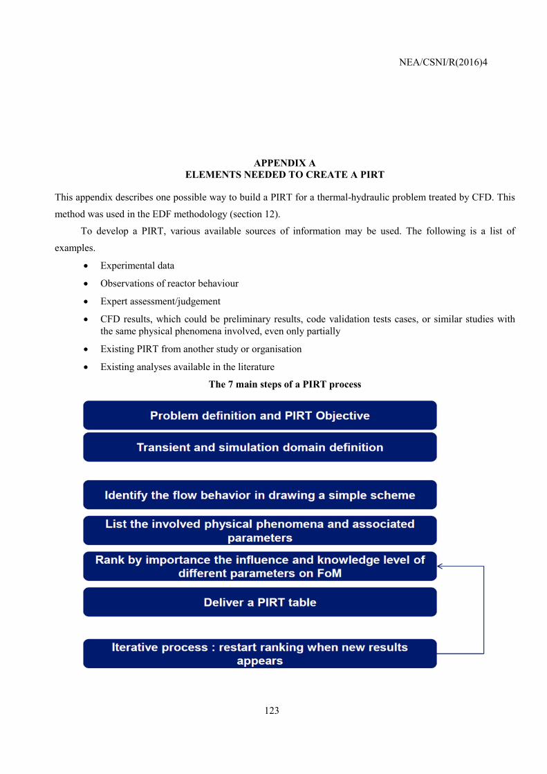
NEA/CSNI/R(2016)4

123

APPENDIX A ELEMENTS NEEDED TO CREATE A PIRT

This appendix describes one possible way to build a PIRT for a thermal-hydraulic problem treated by CFD. This

method was used in the EDF methodology (section 12).

To develop a PIRT, various available sources of information may be used. The following is a list of

examples.

• Experimental data

• Observations of reactor behaviour

• Expert assessment/judgement

• CFD results, which could be preliminary results, code validation tests cases, or similar studies with the same physical phenomena involved, even only partially

• Existing PIRT from another study or organisation

• Existing analyses available in the literature

The 7 main steps of a PIRT process

NEA/CSNI/R(2016)4

124

NEA/CSNI/R(2016)4

125

Define what a physical phenomenon is in a problem treated by CFD.

Fluid mechanics deals with various scales, from dissipative turbulent structures to primary loop in a nuclear power plant. This leads to a large variety of possible physical phenomena involved in any problem treated in a CFD study. On the other hand, most phenomena are based on a few physical processes happening at small scales, specifically, inertia, friction, and heat and mass transfer.

First, a definition of a physical phenomenon is necessary in order to establish an objective and determine the scale of interest for describing transients treated by CFD. A physical phenomenon is an observed flow behaviour or a part of the flow behaviour at the scale of interest; combining all identified physical phenomena in a given problem should explain the whole investigated transient. In other words, the list of main physical phenomena involved is a way to exhaustively decompose the flow of interest.

For example, in a PTS, some of the transient physical phenomena are jet impact, thermal stratification, the plume effect, and wall heat transfer. In this example, turbulence and mixing are the main processes but they are too general to be in this list of phenomena.

Define the parameters associated with the physical phenomena identified

To introduce the PIRT table, a simple table identifying phenomena and parameters is suggested.

Discern the dominant parameters (the figures of merit) from the parameters which influence the FoMs

The figures of merit (FoMs) are those parameters that/I don’t know that play a direct and key role on the safety criteria. They are most often imposed by the physics of the transient. Depending on the safety scenario, a FoM can be a scalar or a multi-dimensional value over space and/or time. For any type of FoM, one has to determine a minimum required accuracy. This accuracy threshold has to be kept in mind when assessing the relevance of all steps in the VVUQ process.

The influential parameters are all the physical parameters related/relevant to the physical phenomena involved that have an influence on the FoM. The FoMs and the influential parameters both characterise the physical phenomena occurring in the transient.

The last parameter to identify is the uncertainty in the ranking, which is usually done by scoring the knowledge base, or knowledge level, for the phenomenon of interest. When a phenomenon is identified as being important but the corresponding knowledge level is low, it indicates that more effort must be applied using for example more research support.

Rank the levels of influence and knowledge of the different parameters on the FoM according to importance

Table A-1 is an example of the format the PIRT could take. Table A.1: A sample PIRT

Phenomena: Parameters

Influence Level

Knowledge Level

Justification & Comments

Phenomenon 1 High Medium Parameter 1-a High Low Parameter 1-b Medium Medium Parameter 1-c Medium High

Phenomenon 2 Medium Medium Parameter 2-a Medium Low Parameter 2-b Low Medium

Phenomenon 3 High Parameter 3-a High Low

Justification and/or comments are necessary to give confidence in the rankings.

NEA/CSNI/R(2016)4

126

Non-dimensional Numbers

From the exhaustive list of parameters influencing the main phenomena, it is possible to define the dimensionless numbers describing the transient of interest using the Buckingham Pi-Theorem. First, we have to verify that the non-dimensional numbers cover all the dominant phenomena and parameters involved in the transient. For example, in a physical situation with thermal stratification, two or three non-dimensional numbers from the following list are needed to sufficiently represent the phenomena associated with thermal stratification: the Reynolds number, the Froude number, the Grashof number, and the Rayleigh number or Prandtl number.

Non-dimensional numbers are thus the cornerstone of the definition of relevant experiments and domains of validation, and only a few of the most important numbers associated with a few key physical phenomena in a given situation may be sufficient to describe and quantify complex transients. So, despite a wide range of possible scales and physical phenomena, only a few fundamental processes are playing the most important roles.

Although non-dimensional numbers are very efficient tools in physical analysis, they are only used for comparative purposes with relative values. Physical phenomena happening in pipes and vessels of different plants or at different scales (experimental vs. industrial) can be compared this way. For this reason, the physical analysis and the definition of validation and application domain must be based on both the list of physical phenomena and the values of dimensionless numbers.

NEA/CSNI/R(2016)4

127

NEA/CSNI/R(2016)4

128

APPENDIX B THE CONCEPT OF A VALIDATION TABLE FOR CFD MODELS

Nuclear safety usually establishes stringent requirements for the quality of CFD calculations. Existing methods of quality control and quality assurance have limitations for industrial CFD calculations due to the complex physical processes and geometry of the systems encountered in such calculations.

To solve this problem, OKB “GIDROPRESS” developed some validation approaches, which are based on NEA, AIAA and ASME recommendations as well as on the following considerations:

• Creating a universal model for industrial application is virtually impossible. Therefore, a CFD model can be developed and applied to a well-defined and limited set of parameters of interest 𝑃𝑃1, 𝑃𝑃2, 𝑃𝑃3, …, 𝑃𝑃𝑁𝑁 such as distribution of velocities, temperatures, concentrations; these parameters of interest usually define functionality, safety, reliability, or efficiency of the developed equipment. This set should be defined at the very beginning (for instance, within the PIRT).

• A model provides a reliable result only in the validated range of the object’s geometric parameters 𝑝𝑝1, 𝑝𝑝2, 𝑝𝑝3, …, 𝑝𝑝𝑆𝑆 (e.g. nominal size, wall roughness, manufacturing tolerances, thermal expansions) and thermal-hydraulic parameters (fluid properties, operating temperatures and pressures, etc., with 𝑝𝑝1𝑛𝑛𝑖𝑖𝑛𝑛 ≤ 𝑝𝑝1 ≤ 𝑝𝑝1𝑛𝑛𝑣𝑣𝑒𝑒, 𝑝𝑝2𝑛𝑛𝑖𝑖𝑛𝑛 ≤ 𝑝𝑝2 ≤ 𝑝𝑝2𝑛𝑛𝑣𝑣𝑒𝑒 where 𝑝𝑝𝑛𝑛𝑣𝑣𝑒𝑒 and 𝑝𝑝𝑛𝑛𝑖𝑖𝑛𝑛 are the upper and lower bounds of the validation range, and S is the total number of object parameters).

• Each validation test must include a preliminary verification step.

• A high-quality experiment is the closest approximation to reality and can be used to define reference values for target parameters.

• The CFD code developer is responsible for model validation, incl. physical models and numerical schemes, in the framework of code V&V, which must be properly documented.

When using commercial codes (ANSYS-CFX, STAR-CCM +, STAR-CD, etc.),validating models for some physical phenomena such as the development and destruction of the hydrodynamic boundary layer, the development of a thermal boundary layer is often unnecessary. If new physical models need to be developed and/or if the validation conducted by the code developer is not sufficient, the user might need to conduct additional validation of these models using (i) adequate experimental data, (ii)the results of DNS calculations, or (iii) analytical solutions, if available. As a result, for considered physical models the maximum deviations of the calculation results compared to experimental or other data for each parameter of interest could be estimated ∆PNmax(fi) = max ∆PN (fi) with i = 1, 2, 3, … , k. If ∆PNmax(fi) exceeds the validated values, to the model must be improved or refined.

As part of the methodology developed by OKB “GIDROPRESS”, the object should be split into several levels of less complex subsystems. For each subsystem, corresponding experimental or other data should be defined for subsystem model validation. Let 𝑛𝑛 be the number of tests for each subsystem sufficient to validate the modelling of the physical phenomena taking place in the subsystem. Since it is often not possible to find a test universal enough for validation of a subsystem by all parameters of interest in the required range of parameters of the object, 𝑛𝑛 is usually greater than 1. In some cases, the transformation of dimensional parameters into dimensionless forms reduces the amount of required validation studies and makes finding adequate experimental data for validation easier. In this case, the number and nomenclature of the dimensionless parameters (e.g. 𝜁𝜁, 𝑁𝑁𝑢𝑢,

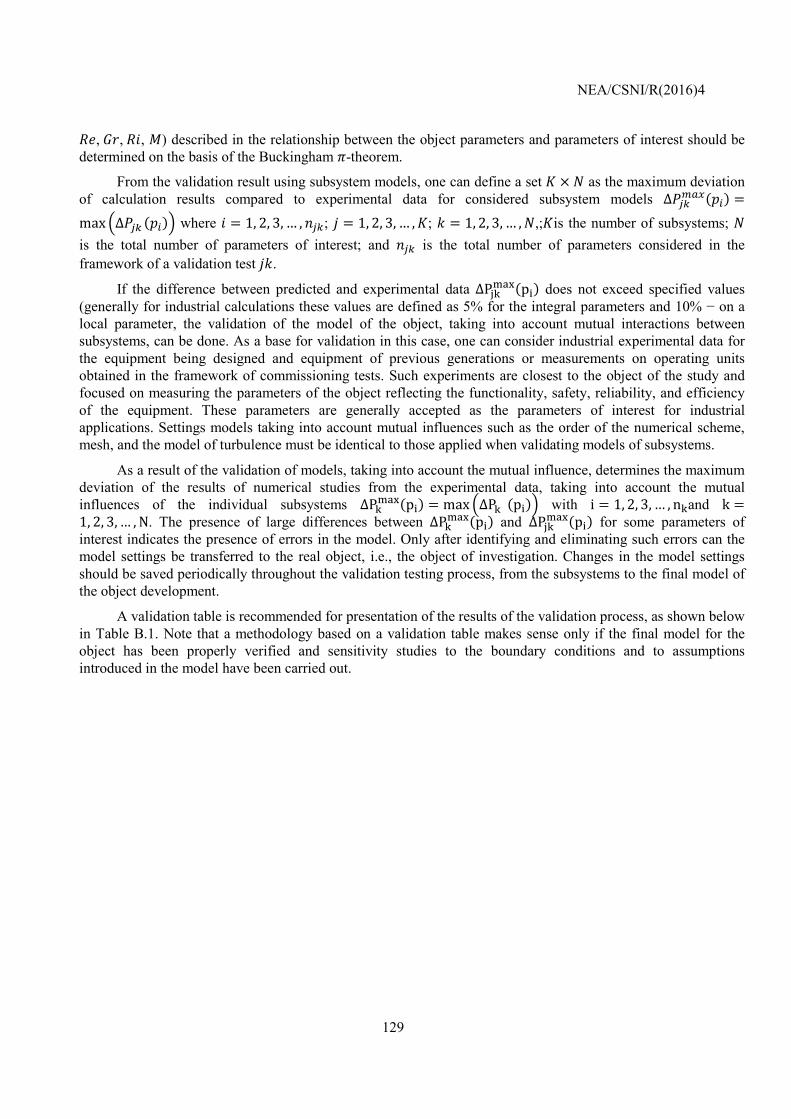
NEA/CSNI/R(2016)4

129

𝑅𝑅𝑒𝑒, 𝐺𝐺𝑟𝑟, 𝑅𝑅𝑚𝑚, 𝑀𝑀) described in the relationship between the object parameters and parameters of interest should be determined on the basis of the Buckingham 𝜋𝜋-theorem.

From the validation result using subsystem models, one can define a set 𝐾𝐾 × 𝑁𝑁 as the maximum deviation of calculation results compared to experimental data for considered subsystem models ∆𝑃𝑃𝑗𝑗𝑘𝑘𝑛𝑛𝑣𝑣𝑒𝑒(𝑝𝑝𝑖𝑖) =max ∆𝑃𝑃𝑗𝑗𝑘𝑘 (𝑝𝑝𝑖𝑖) where 𝑚𝑚 = 1, 2, 3, … ,𝑛𝑛𝑗𝑗𝑘𝑘; 𝑗𝑗 = 1, 2, 3, … ,𝐾𝐾; 𝑘𝑘 = 1, 2, 3, … ,𝑁𝑁,;𝐾𝐾is the number of subsystems; 𝑁𝑁 is the total number of parameters of interest; and 𝑛𝑛𝑗𝑗𝑘𝑘 is the total number of parameters considered in the framework of a validation test 𝑗𝑗𝑘𝑘.

If the difference between predicted and experimental data ∆Pjkmax(pi) does not exceed specified values (generally for industrial calculations these values are defined as 5% for the integral parameters and 10% − on a local parameter, the validation of the model of the object, taking into account mutual interactions between subsystems, can be done. As a base for validation in this case, one can consider industrial experimental data for the equipment being designed and equipment of previous generations or measurements on operating units obtained in the framework of commissioning tests. Such experiments are closest to the object of the study and focused on measuring the parameters of the object reflecting the functionality, safety, reliability, and efficiency of the equipment. These parameters are generally accepted as the parameters of interest for industrial applications. Settings models taking into account mutual influences such as the order of the numerical scheme, mesh, and the model of turbulence must be identical to those applied when validating models of subsystems.

As a result of the validation of models, taking into account the mutual influence, determines the maximum deviation of the results of numerical studies from the experimental data, taking into account the mutual influences of the individual subsystems ∆Pkmax(pi) = max ∆Pk (pi) with i = 1, 2, 3, … , nkand k =1, 2, 3, … , N. The presence of large differences between ∆Pkmax(pi) and ∆Pjkmax(pi) for some parameters of interest indicates the presence of errors in the model. Only after identifying and eliminating such errors can the model settings be transferred to the real object, i.e., the object of investigation. Changes in the model settings should be saved periodically throughout the validation testing process, from the subsystems to the final model of the object development.

A validation table is recommended for presentation of the results of the validation process, as shown below in Table B.1. Note that a methodology based on a validation table makes sense only if the final model for the object has been properly verified and sensitivity studies to the boundary conditions and to assumptions introduced in the model have been carried out.

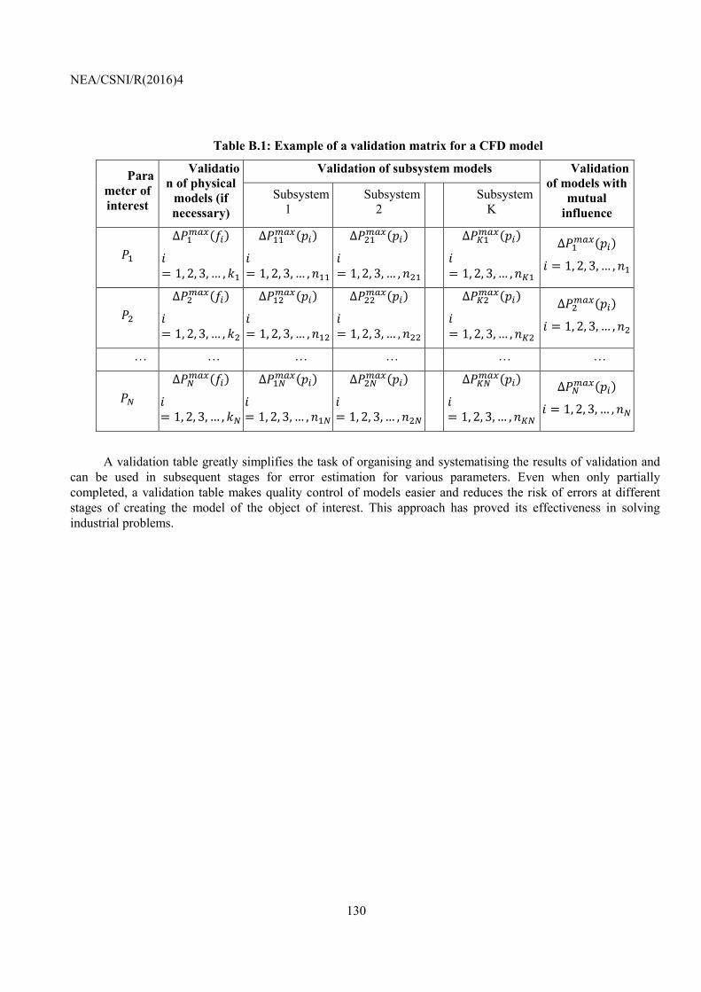
NEA/CSNI/R(2016)4

130

Table B.1: Example of a validation matrix for a CFD model

Parameter of interest

Validation of physical

models (if necessary)

Validation of subsystem models Validation of models with

mutual influence

Subsystem 1

Subsystem 2 Subsystem

K

𝑃𝑃1 ∆𝑃𝑃1𝑛𝑛𝑣𝑣𝑒𝑒(𝑓𝑓𝑖𝑖)

𝑚𝑚= 1, 2, 3, … ,𝑘𝑘1

∆𝑃𝑃11𝑛𝑛𝑣𝑣𝑒𝑒(𝑝𝑝𝑖𝑖)

𝑚𝑚= 1, 2, 3, … ,𝑛𝑛11

∆𝑃𝑃21𝑛𝑛𝑣𝑣𝑒𝑒(𝑝𝑝𝑖𝑖)

𝑚𝑚= 1, 2, 3, … ,𝑛𝑛21

∆𝑃𝑃𝐾𝐾1𝑛𝑛𝑣𝑣𝑒𝑒(𝑝𝑝𝑖𝑖)

𝑚𝑚= 1, 2, 3, … ,𝑛𝑛𝐾𝐾1

∆𝑃𝑃1𝑛𝑛𝑣𝑣𝑒𝑒(𝑝𝑝𝑖𝑖)

𝑚𝑚 = 1, 2, 3, … ,𝑛𝑛1

𝑃𝑃2 ∆𝑃𝑃2𝑛𝑛𝑣𝑣𝑒𝑒(𝑓𝑓𝑖𝑖)

𝑚𝑚= 1, 2, 3, … , 𝑘𝑘2

∆𝑃𝑃12𝑛𝑛𝑣𝑣𝑒𝑒(𝑝𝑝𝑖𝑖)

𝑚𝑚= 1, 2, 3, … ,𝑛𝑛12

∆𝑃𝑃22𝑛𝑛𝑣𝑣𝑒𝑒(𝑝𝑝𝑖𝑖)

𝑚𝑚= 1, 2, 3, … ,𝑛𝑛22

∆𝑃𝑃𝐾𝐾2𝑛𝑛𝑣𝑣𝑒𝑒(𝑝𝑝𝑖𝑖)

𝑚𝑚= 1, 2, 3, … ,𝑛𝑛𝐾𝐾2

∆𝑃𝑃2𝑛𝑛𝑣𝑣𝑒𝑒(𝑝𝑝𝑖𝑖)

𝑚𝑚 = 1, 2, 3, … ,𝑛𝑛2

… … … … … …

𝑃𝑃𝑁𝑁 ∆𝑃𝑃𝑁𝑁𝑛𝑛𝑣𝑣𝑒𝑒(𝑓𝑓𝑖𝑖)

𝑚𝑚= 1, 2, 3, … ,𝑘𝑘𝑁𝑁

∆𝑃𝑃1𝑁𝑁𝑛𝑛𝑣𝑣𝑒𝑒(𝑝𝑝𝑖𝑖)

𝑚𝑚= 1, 2, 3, … ,𝑛𝑛1𝑁𝑁

∆𝑃𝑃2𝑁𝑁𝑛𝑛𝑣𝑣𝑒𝑒(𝑝𝑝𝑖𝑖)

𝑚𝑚= 1, 2, 3, … ,𝑛𝑛2𝑁𝑁

∆𝑃𝑃𝐾𝐾𝑁𝑁𝑛𝑛𝑣𝑣𝑒𝑒(𝑝𝑝𝑖𝑖)

𝑚𝑚= 1, 2, 3, … ,𝑛𝑛𝐾𝐾𝑁𝑁

∆𝑃𝑃𝑁𝑁𝑛𝑛𝑣𝑣𝑒𝑒(𝑝𝑝𝑖𝑖)

𝑚𝑚 = 1, 2, 3, … ,𝑛𝑛𝑁𝑁

A validation table greatly simplifies the task of organising and systematising the results of validation and can be used in subsequent stages for error estimation for various parameters. Even when only partially completed, a validation table makes quality control of models easier and reduces the risk of errors at different stages of creating the model of the object of interest. This approach has proved its effectiveness in solving industrial problems.