Embed Size (px)
Citation preview
Review of the Valeo-CD Aerofoil Tests
Clare Turner

Purpose1) Extensive tests have been done on the T3 flat plate tests to
demonstrate abilities to predict transition under high free-stream turbulence intensities ; i.e. testing bypass transition.
2) The 2-D Valeo aerofoil case exhibits transition which is not induced by high free-stream disturbances, which most RANS models cannot predict.
3) This is a step towards the final application of a three dimensional rear wing which undergoes separation.
4) It is also an opportunity to test the models’ performance under a pressure gradient and their abilities to predict pressure coefficient.

The test case set-up: general• The Valeo aerofoil is cambered and thin with an 8°
geometric angle of attack. The maximum thickness of 4.5% of the chord length.
• The experiments showed that turbulence from the jet quickly dissipated away; so a very small value of k was chosen at the inlet.
• The cells are reported as y+ < 1 and x+ ≤ 20, with one cell in the z direction. There are 80,808 cells in total.
• The geometry and viscosity are scaled to give a unit chord and a free-stream velocity of 1ms-1.
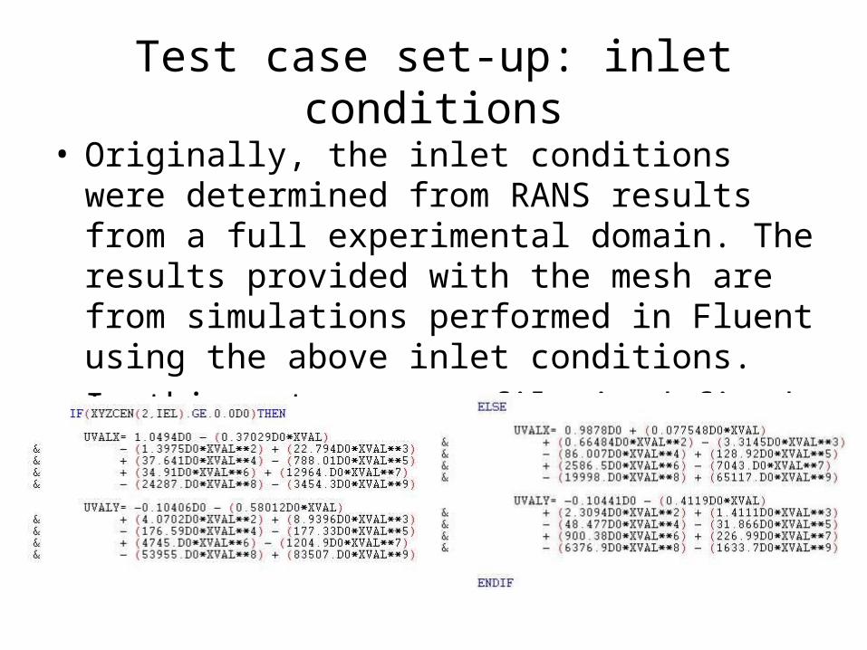
Test case set-up: inlet conditions
• Originally, the inlet conditions were determined from RANS results from a full experimental domain. The results provided with the mesh are from simulations performed in Fluent using the above inlet conditions.
• In this set-up a profile is defined with the following equations:

Validating the set-up• Comparing the provided v2-f results with those from star-CD
and Code_Saturne is useful as validation of the different codes and versions of the models
• The v2-f comparisons are mainly used here to indicate any errors in the set-up
• Experimental, v2-f and LES results of pressure coefficients and 8 wake profiles were provided with the mesh
• The following results show that the v2-f results are similar from all three codes, if anything the results from Saturne and Star-CD are closer to the experimental than those provided
• Results from the two kT-kL-ω models in Saturne are also included in the figures
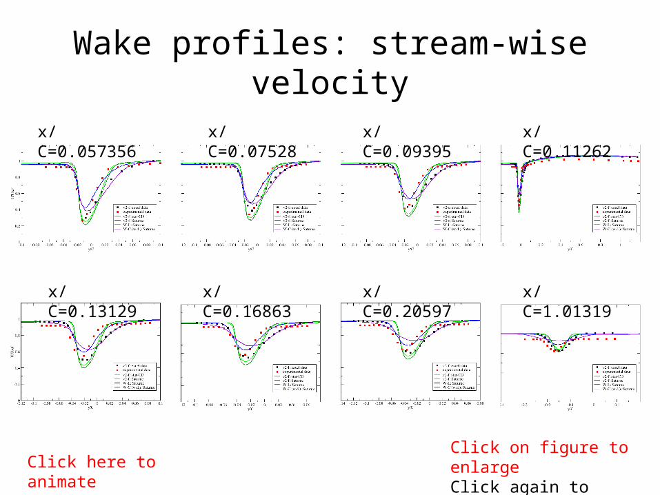
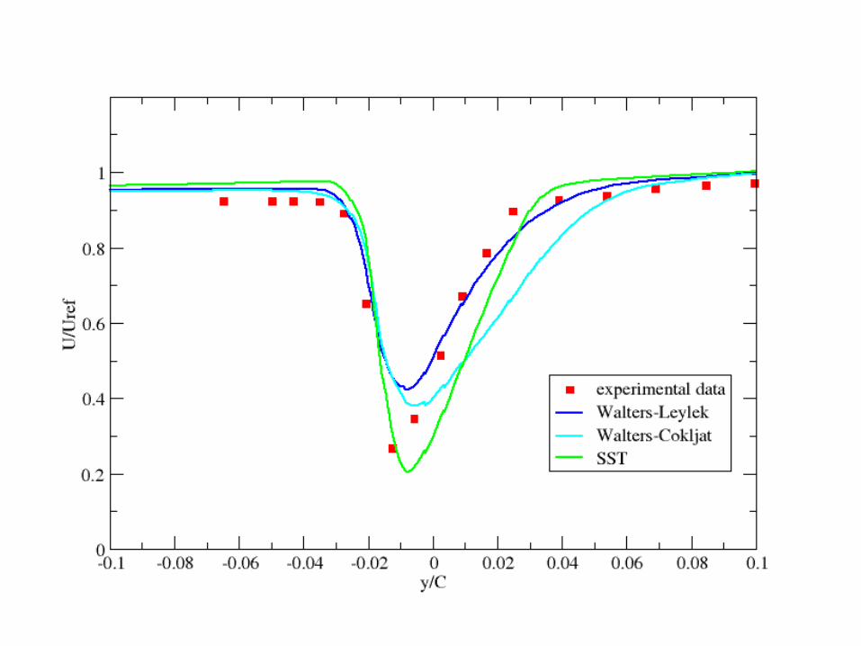
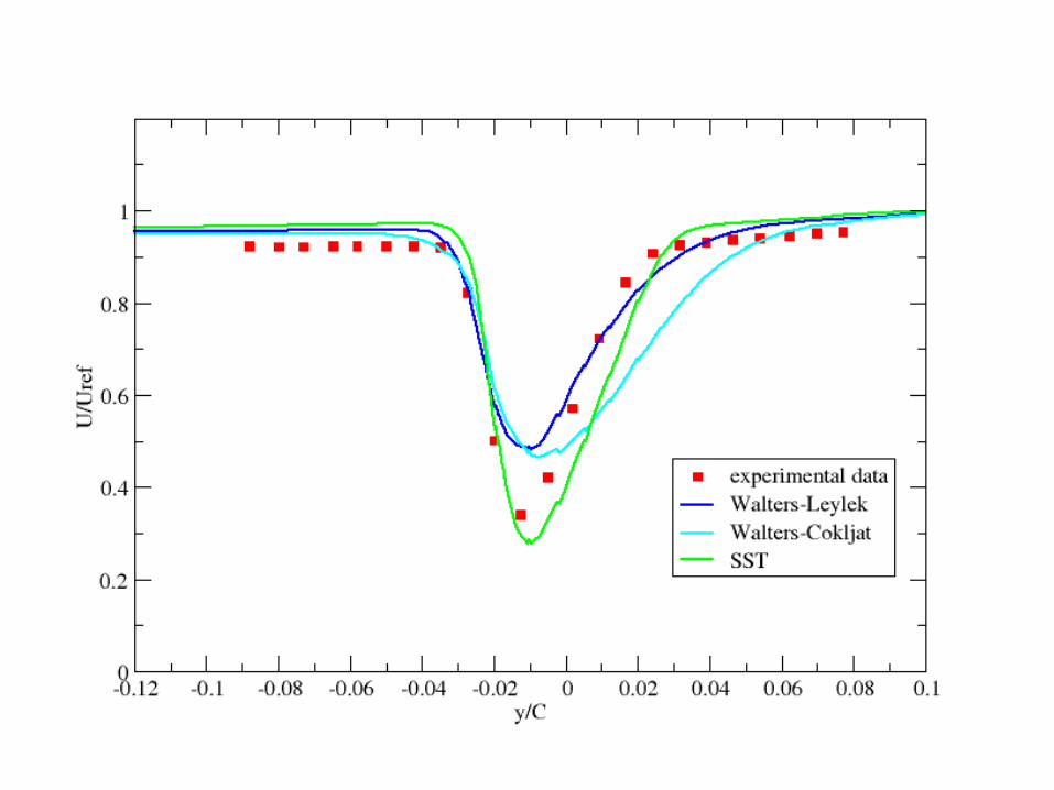
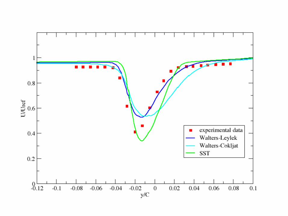
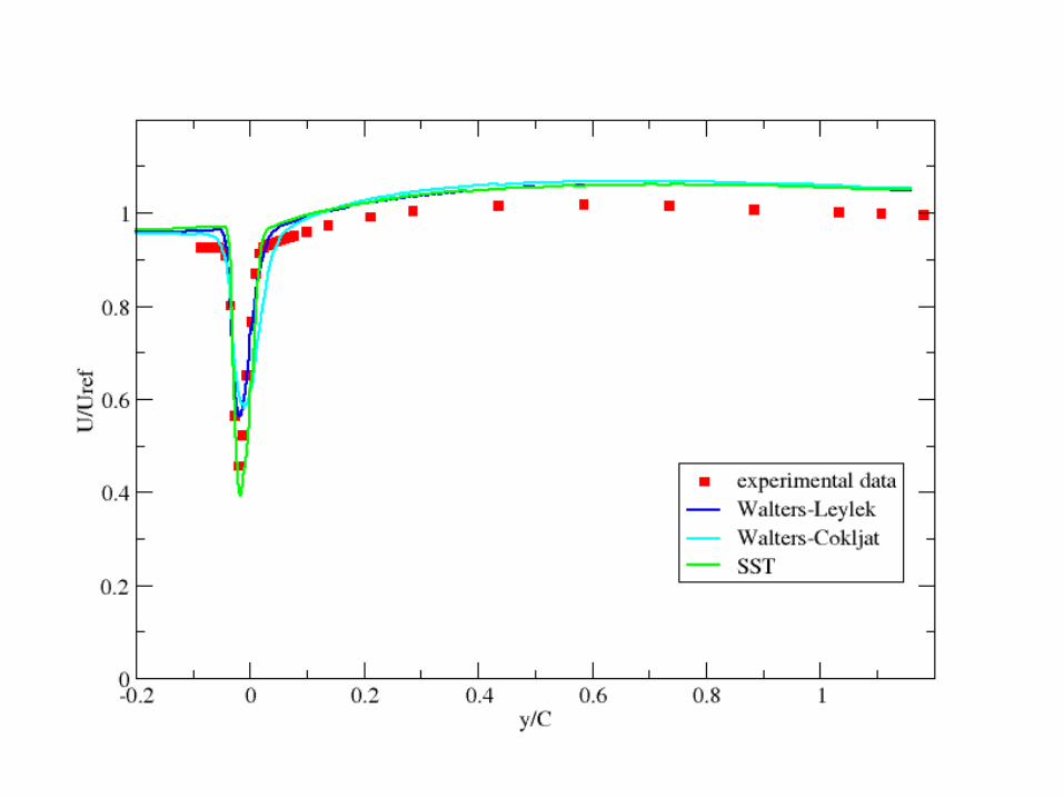
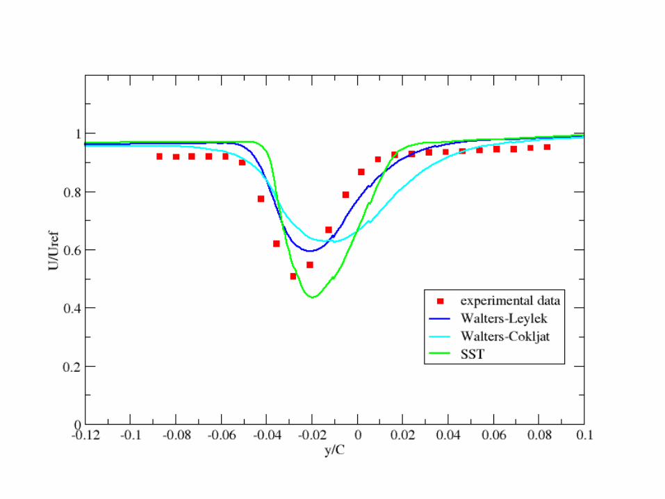
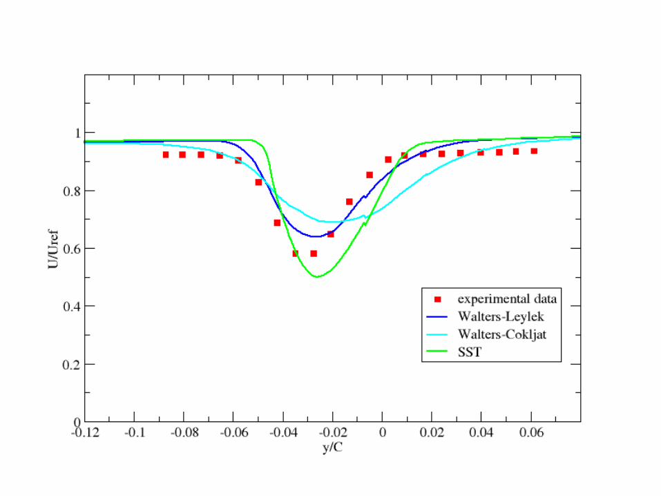
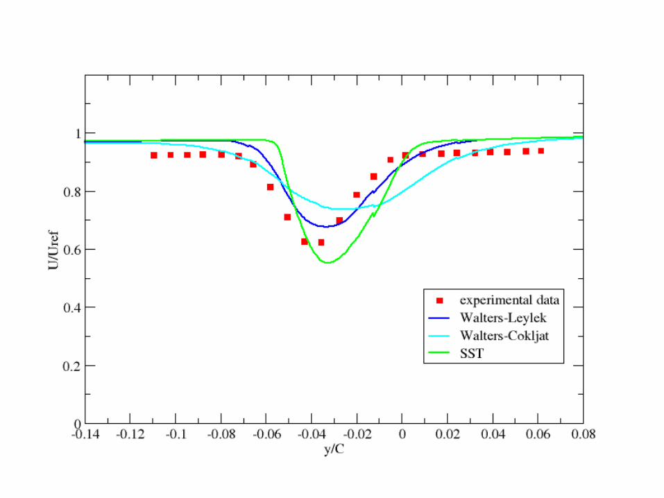
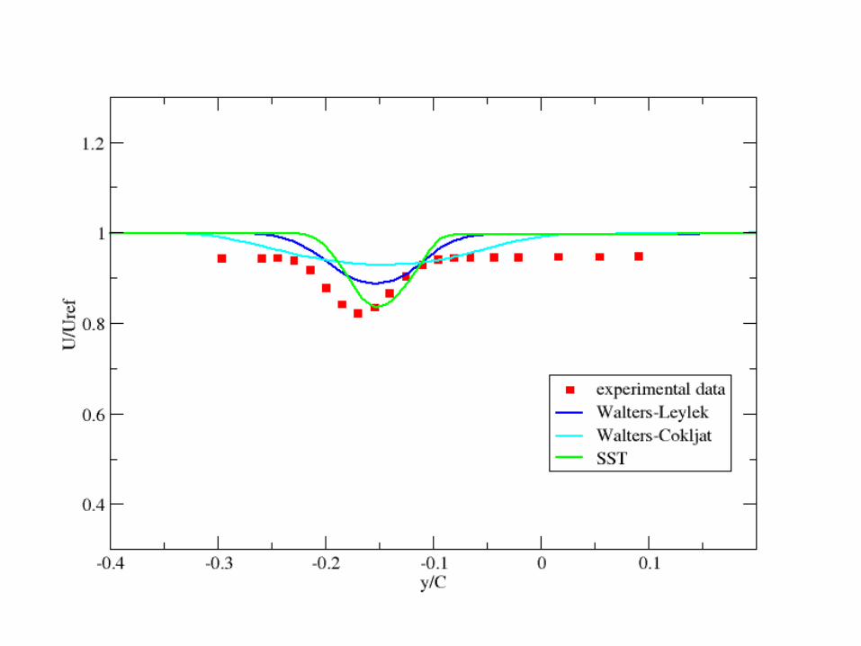
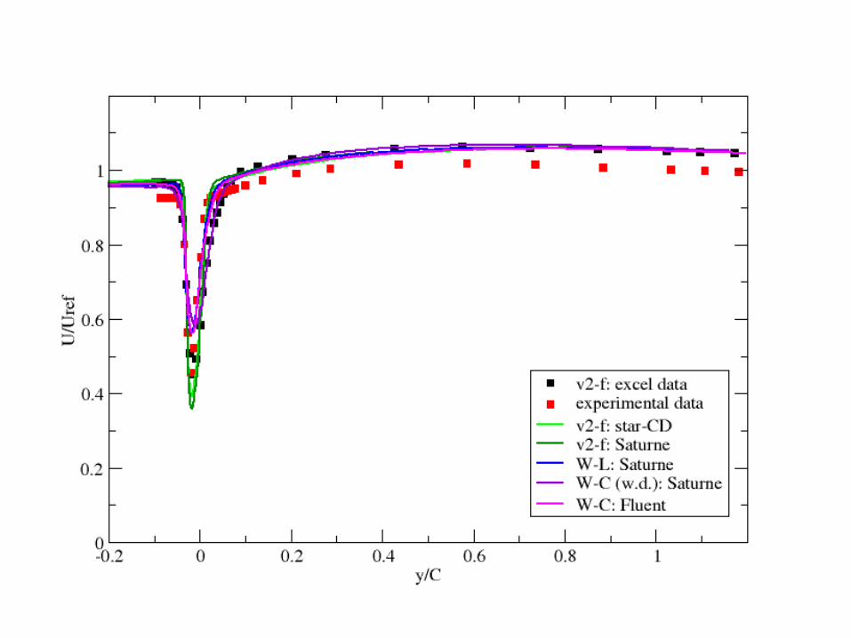
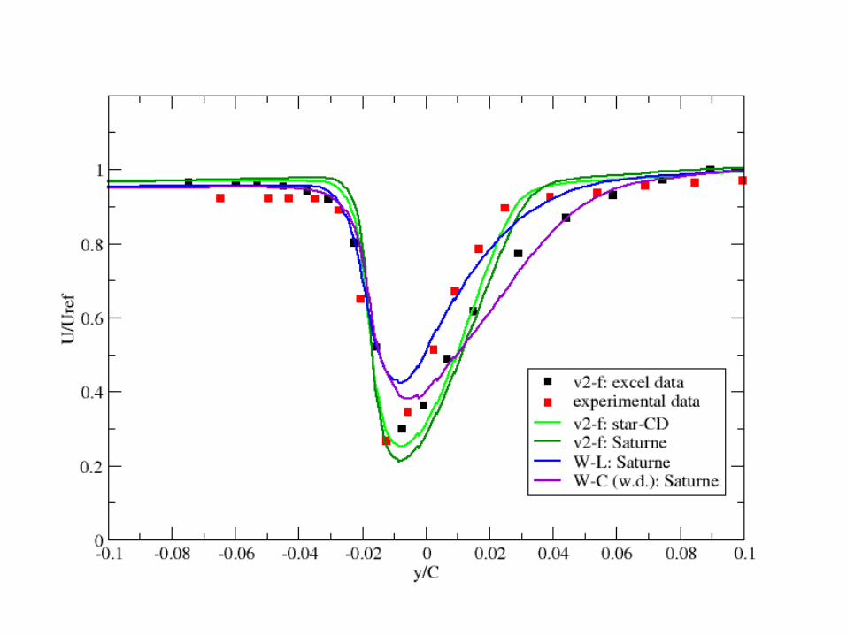
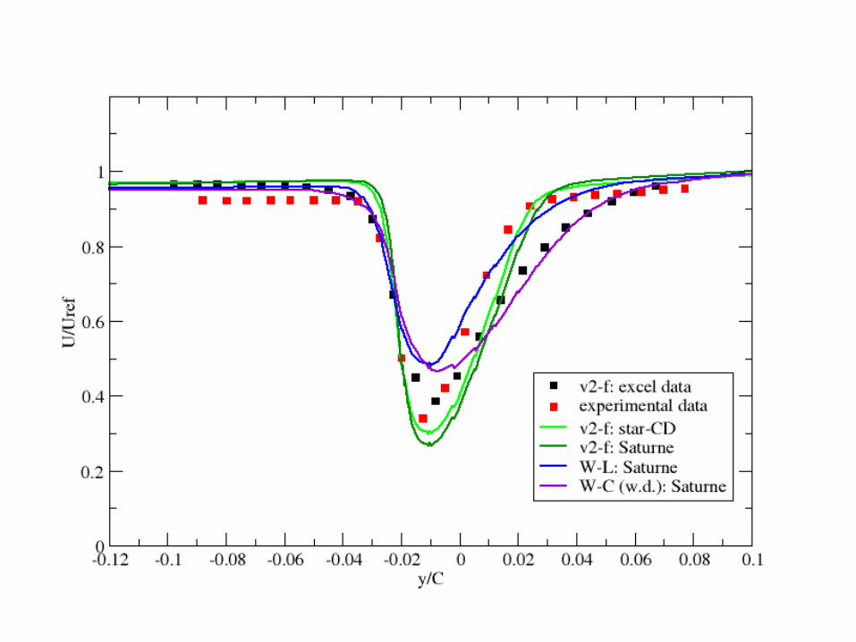
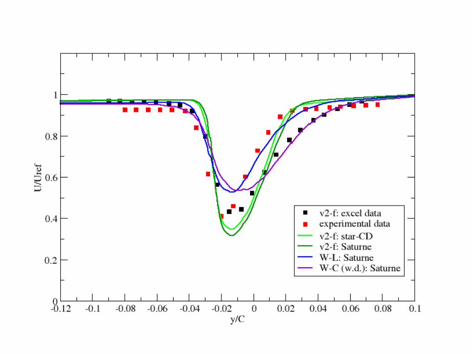
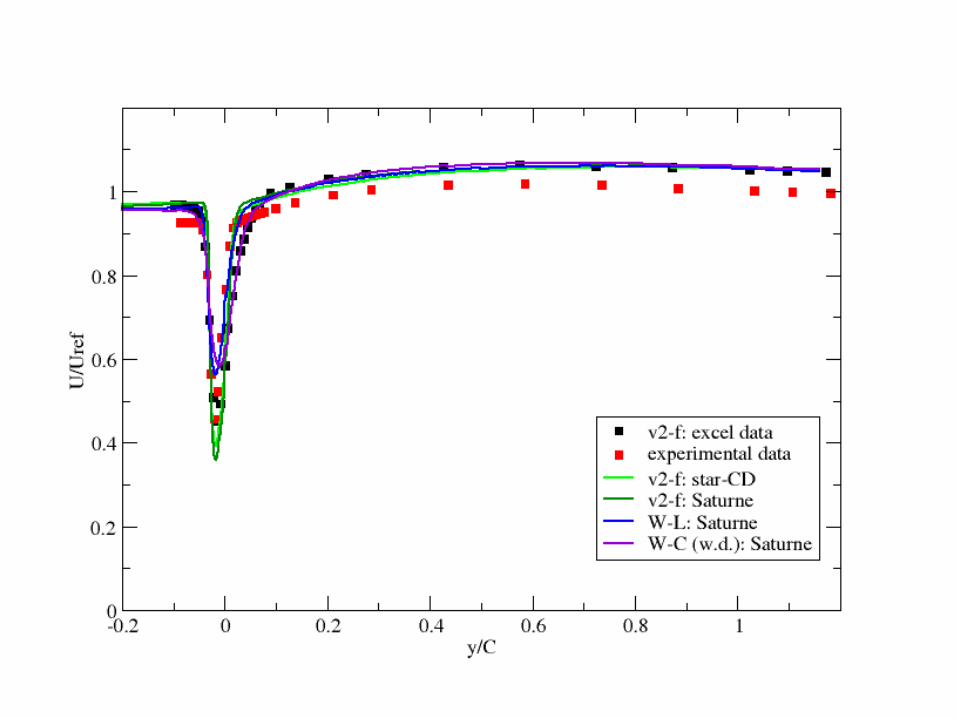
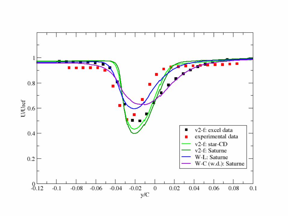
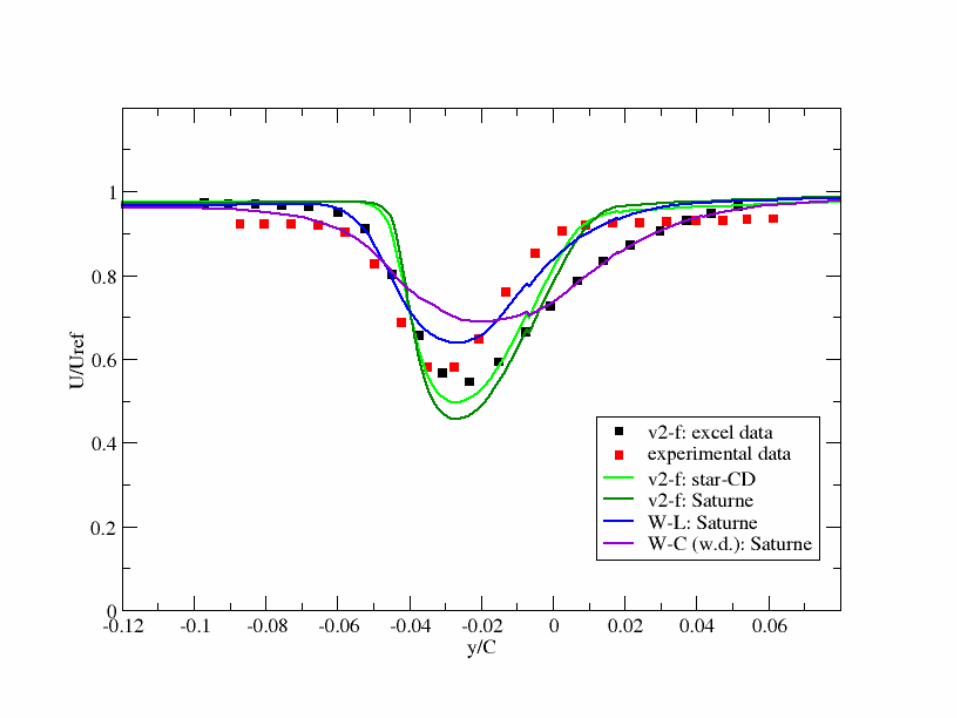
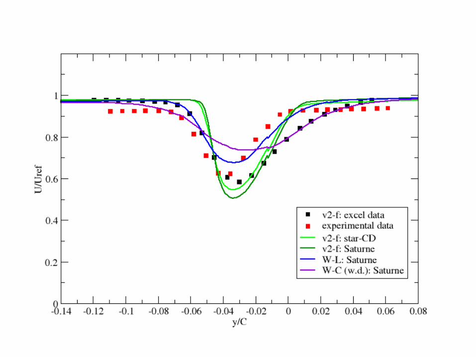
Wake profiles: stream-wise velocity
x/C=0.07528x/C=0.057356 x/C=0.09395 x/C=0.11262
x/C=0.13129 x/C=0.16863 x/C=0.20597 x/C=1.01319
Click on figure to enlargeClick again to returnClick here to animate

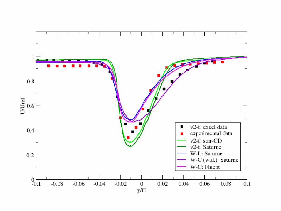
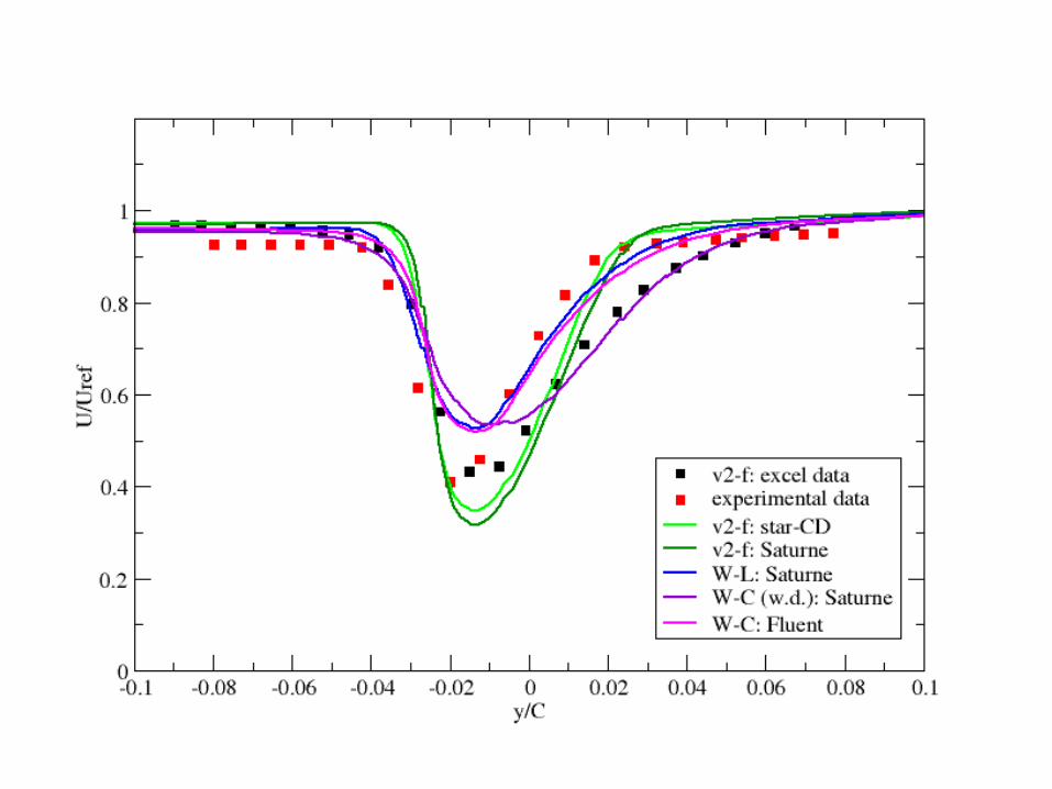
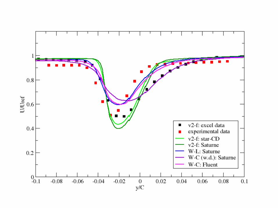
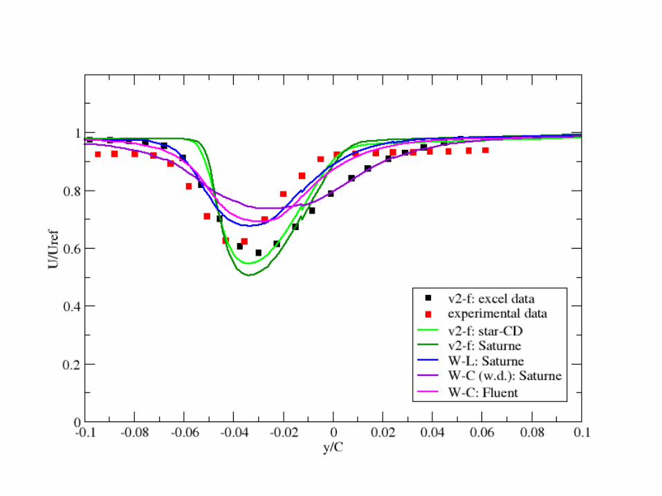
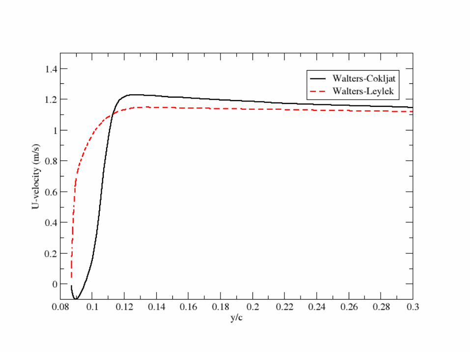
Model Comparisons – wake profiles (U)• There are two main differences between the v2-f models and
the experimental results for the wake profiles: the minimum U-component of the velocity in the wake is noticeably lower; the free-stream velocity is too high. The latter can be explained by an over prediction of the inlet velocities.
• The kT-kL-ω models have the opposite problem to the v2-f models in that the minimum velocity is too high.
• Other than this the Walters-Leylek profile is close to the experimental results.
• The Walters-Cokljat model deviates both in the location of the centre of the wake and the velocity at that point.
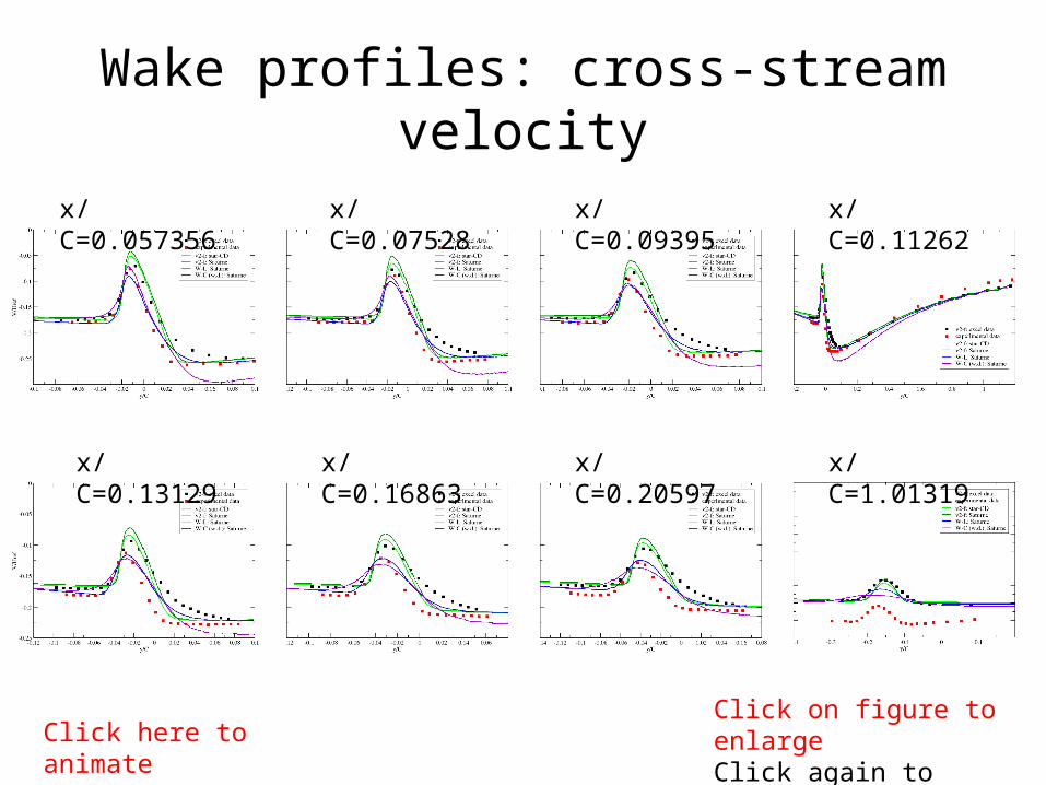
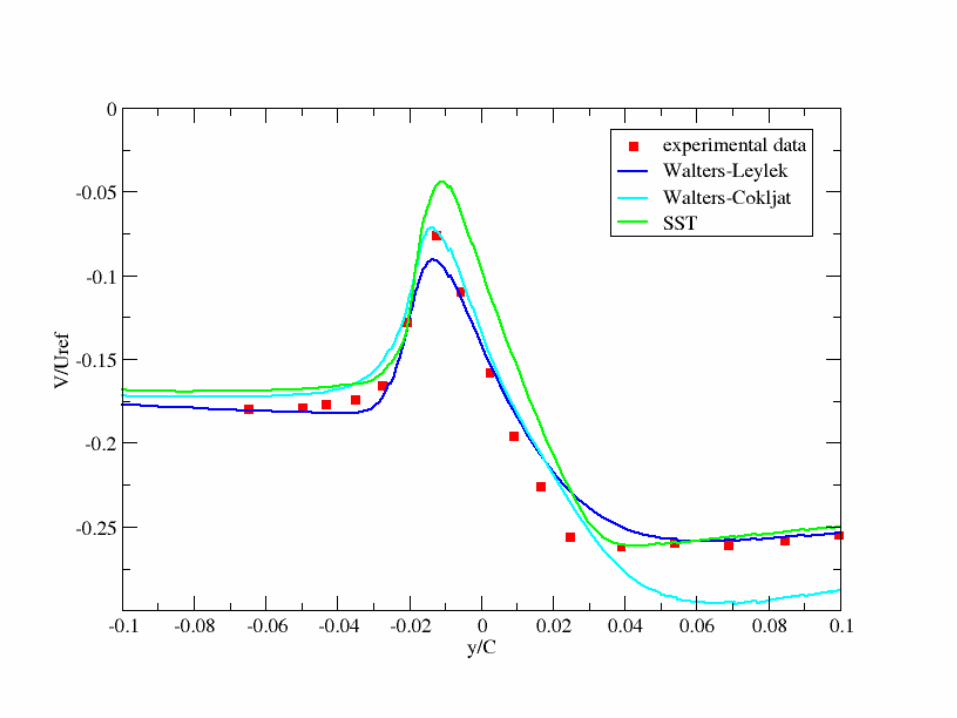
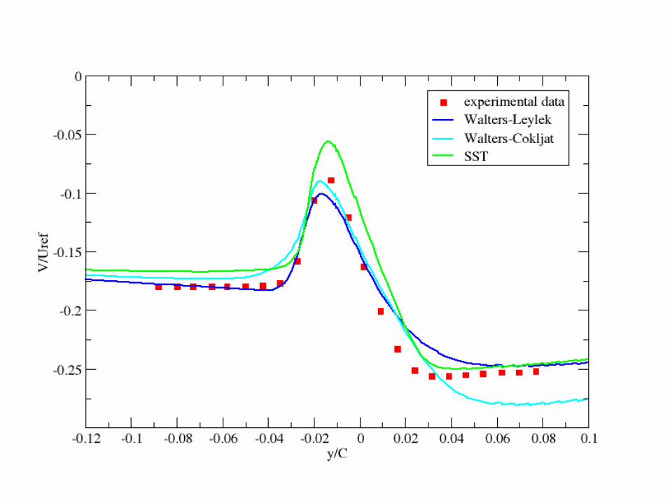
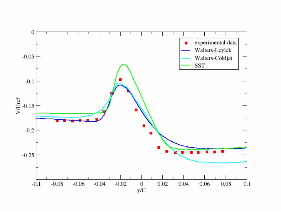
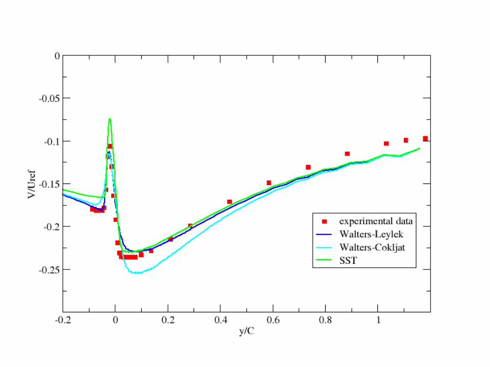
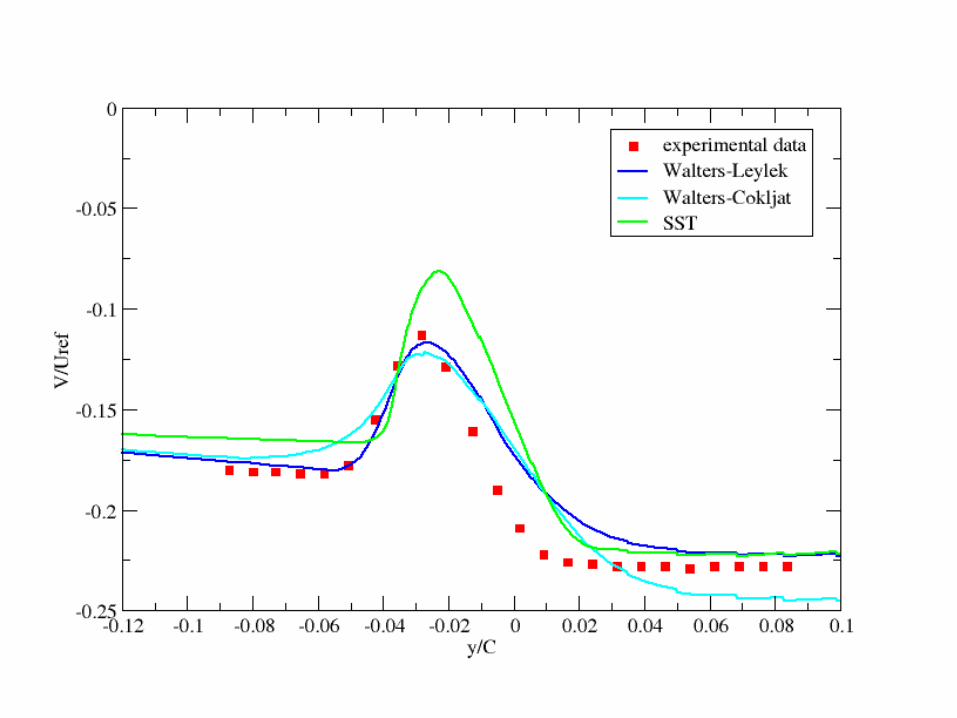
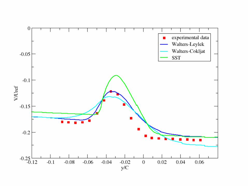
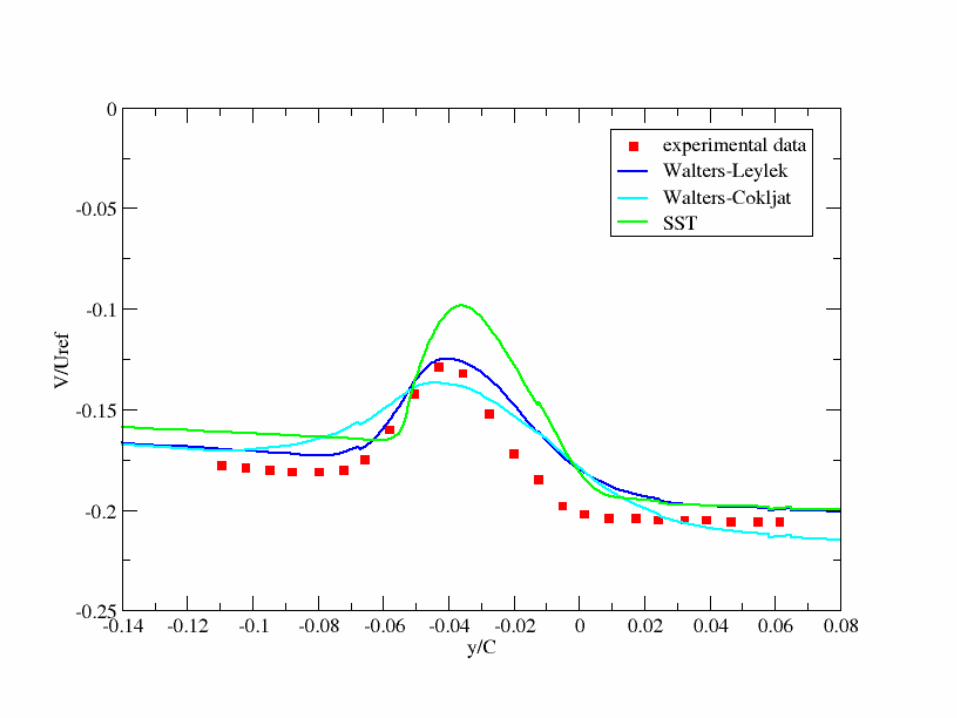
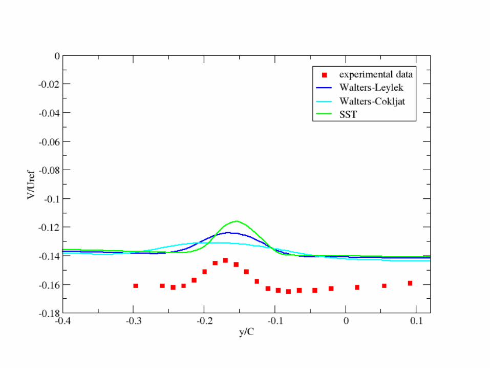
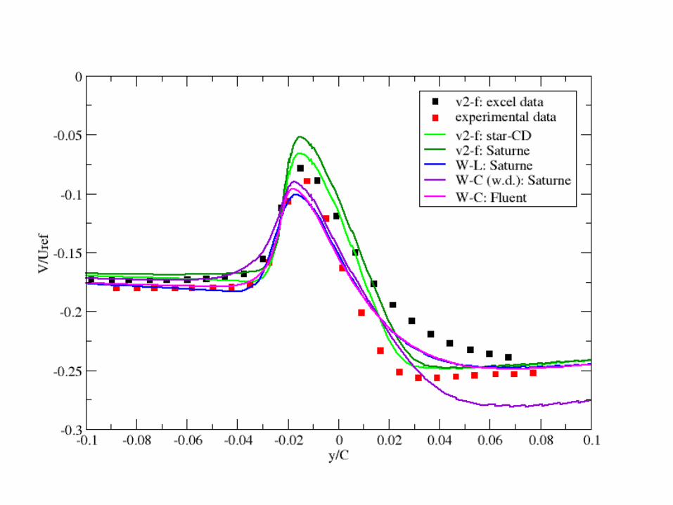
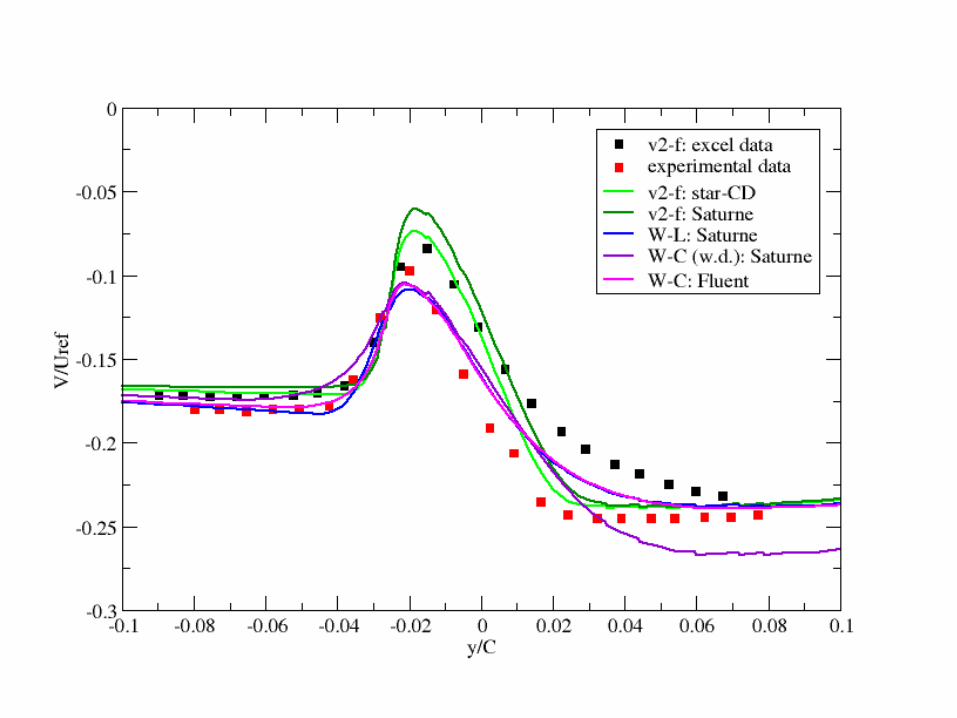
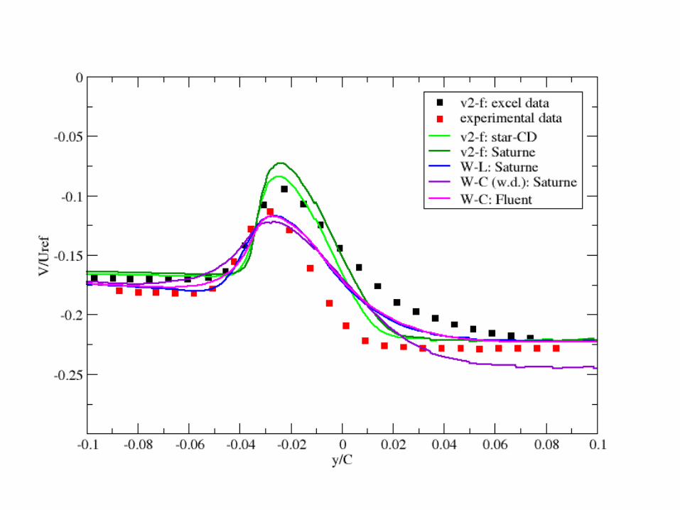
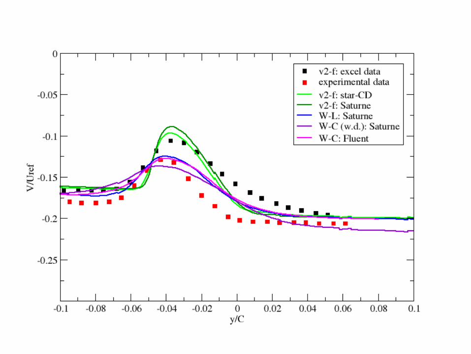
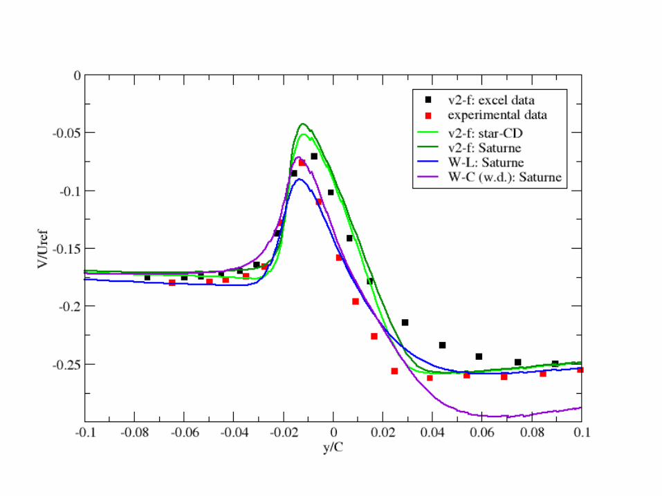
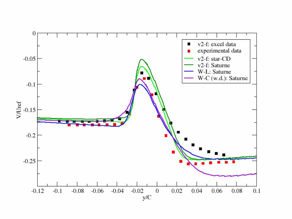
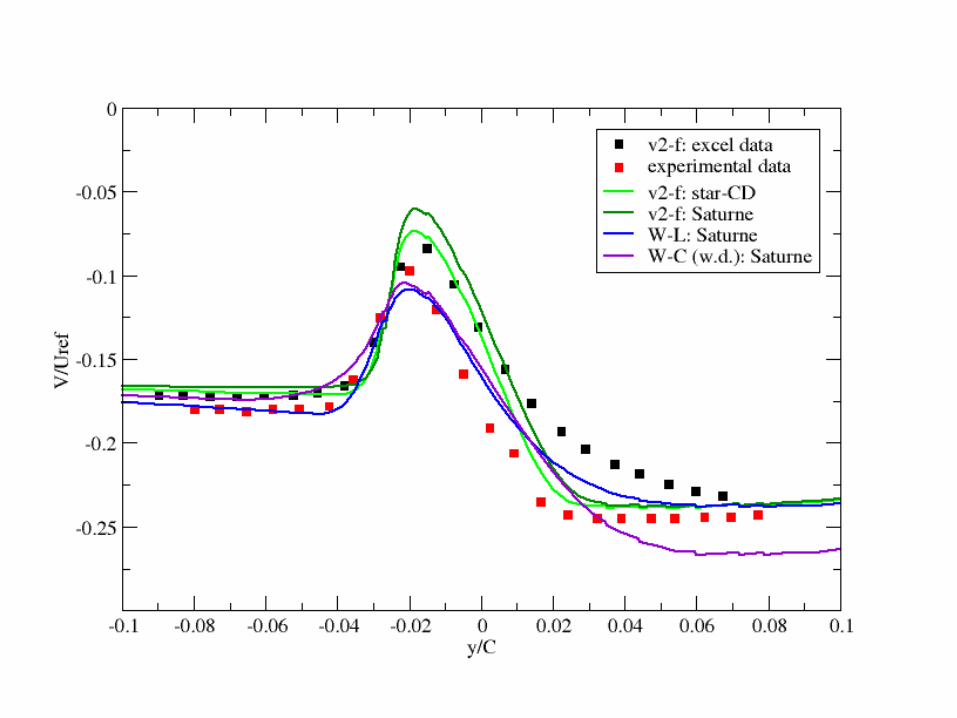
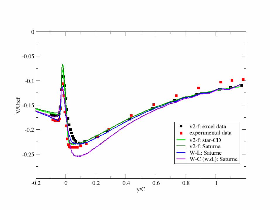
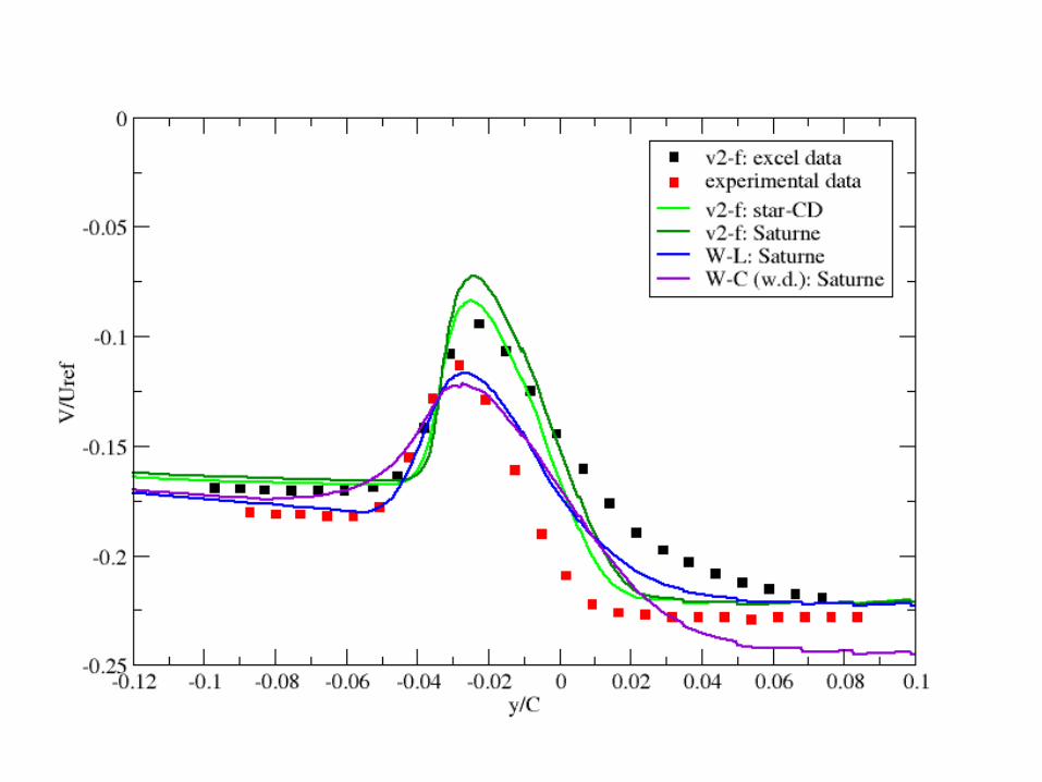
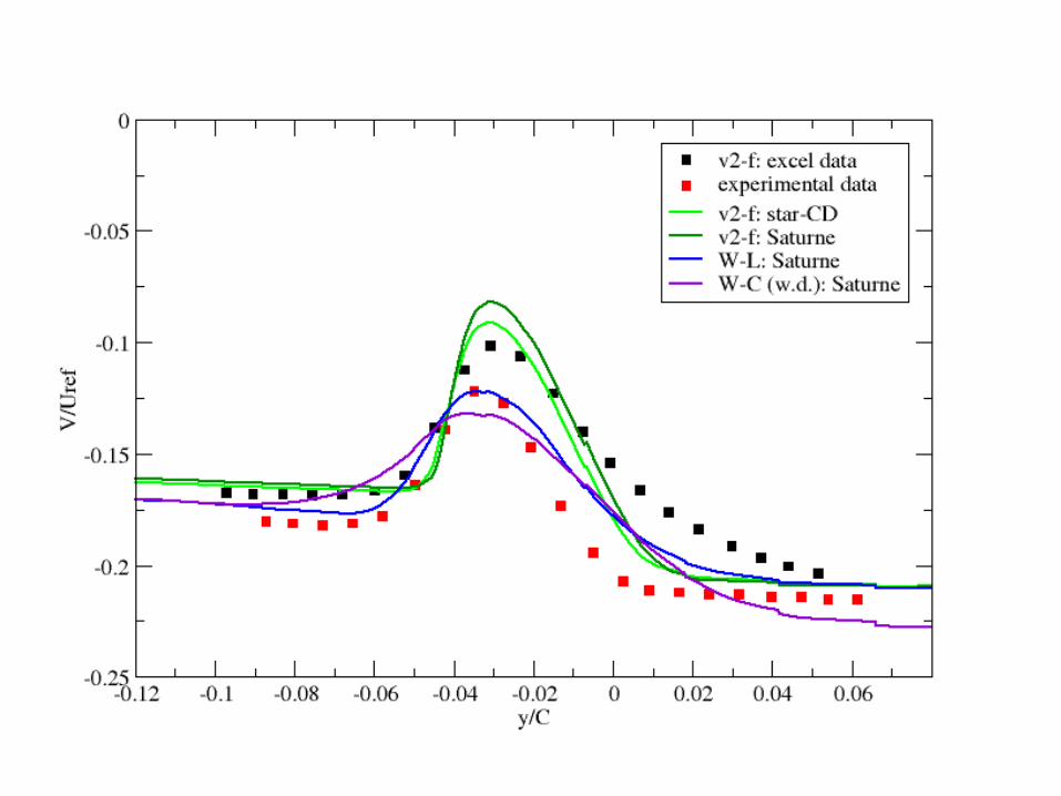
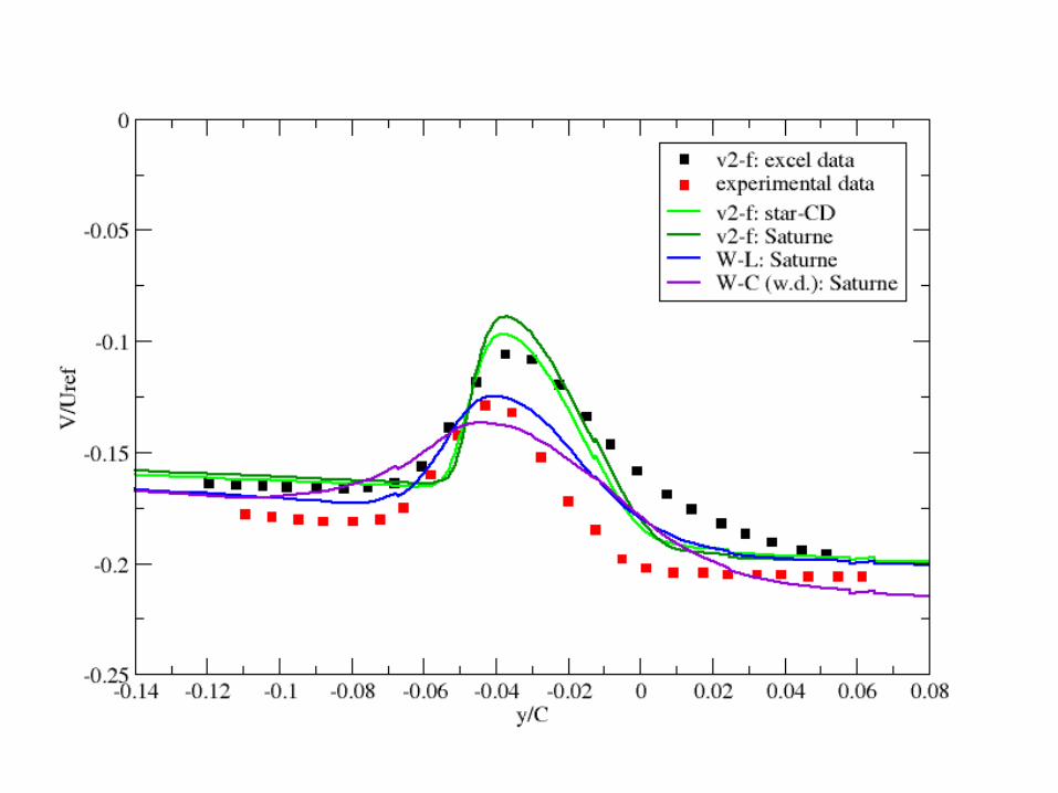
Wake profiles: cross-stream velocity
Click here to animate
x/C=0.20597 x/C=1.01319x/C=0.16863x/C=0.13129
x/C=0.057356 x/C=0.07528 x/C=0.09395 x/C=0.11262
Click on figure to enlargeClick again to return
Model Comparisons – wake profiles (V)• The outcome is similar, in that the magnitude of the velocity
deficit is too large for the v2-f models and too small for the kT-kL-ω models. However, the Walters-Leylek model is very close to the experimental values.
• The Walters-Cokljat model deviates from expected values towards the free-stream.
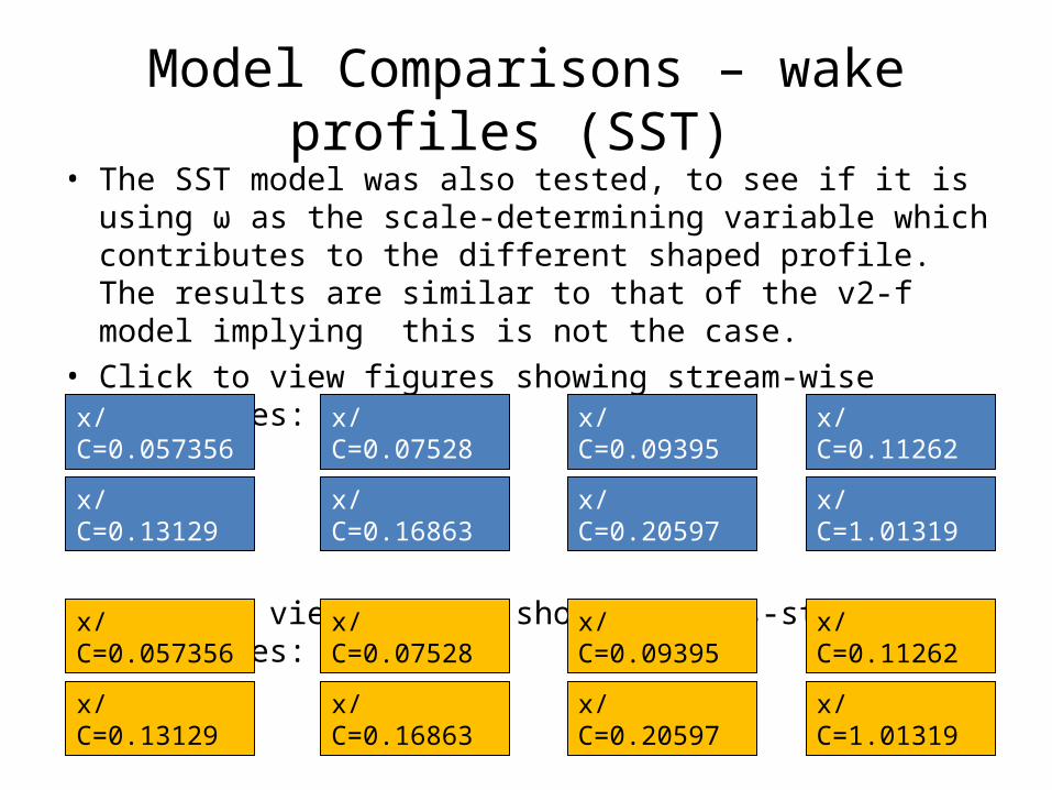
Model Comparisons – wake profiles (SST) • The SST model was also tested, to see if it is using ω as the
scale-determining variable which contributes to the different shaped profile. The results are similar to that of the v2-f model implying this is not the case.
• Click to view figures showing stream-wise velocities:
• Click to view figures showing cross-stream velocities:
x/C=0.20597 x/C=1.01319x/C=0.16863x/C=0.13129
x/C=0.057356 x/C=0.07528 x/C=0.09395 x/C=0.11262
x/C=0.20597 x/C=1.01319x/C=0.16863x/C=0.13129
x/C=0.057356 x/C=0.07528 x/C=0.09395 x/C=0.11262
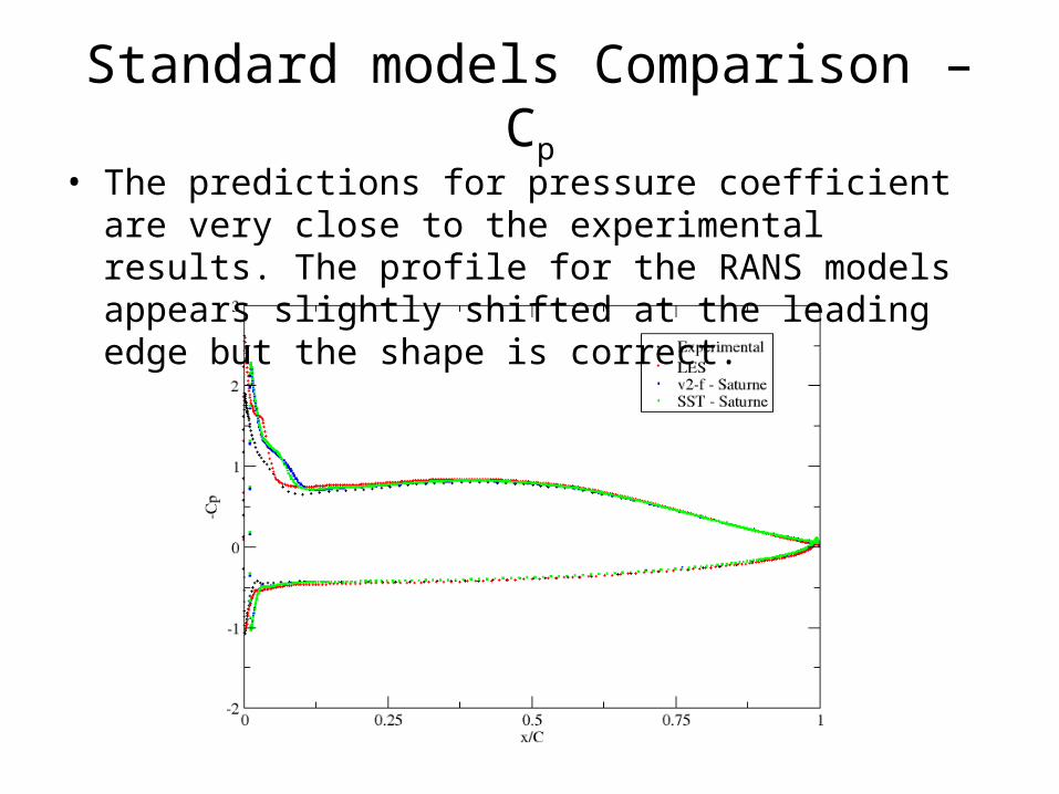
Standard models Comparison – Cp
• The predictions for pressure coefficient are very close to the experimental results. The profile for the RANS models appears slightly shifted at the leading edge but the shape is correct.
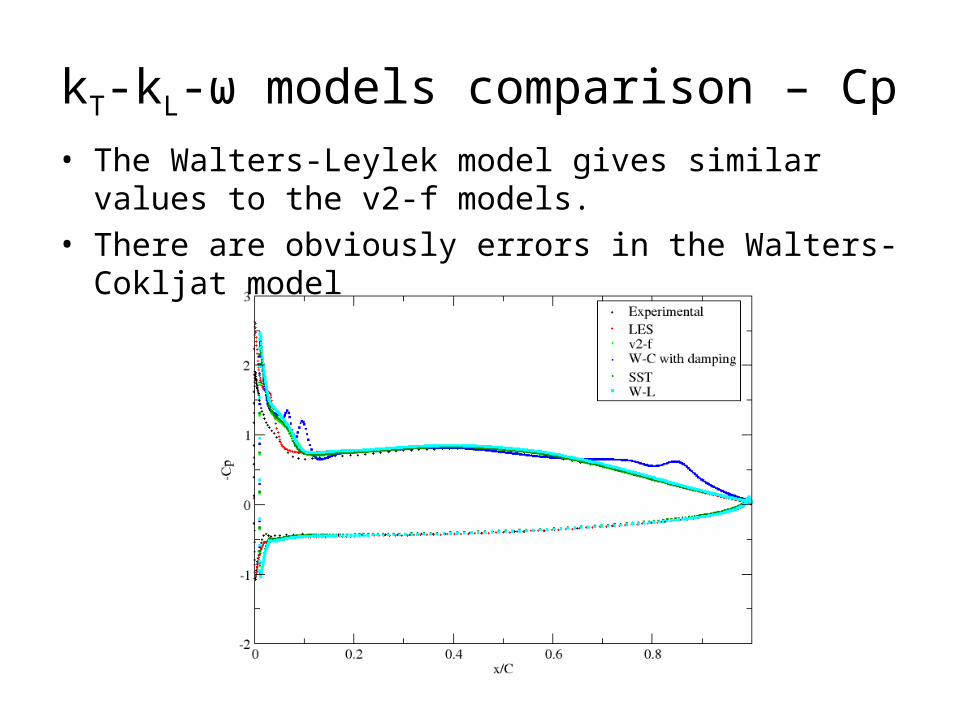
kT-kL-ω models comparison – Cp• The Walters-Leylek model gives similar values to the v2-f
models. • There are obviously errors in the Walters-Cokljat model

Contours of turbulence• The turbulent kinetic energy should be present on the suction
side of the aerofoil after the separation bubble and in the wake, as presented in the Walters-Leylek contours.
• Transition occurs much later than expected in the Walters-Cokljat model.
Walters-Cokljat Walters-Leylek
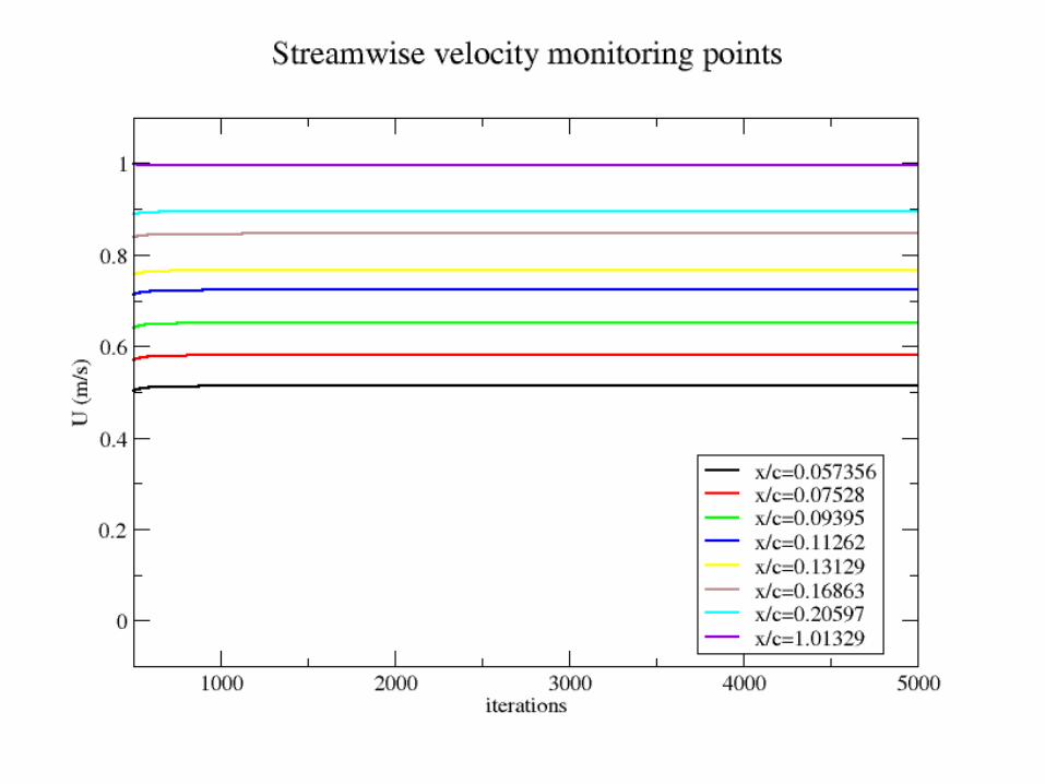
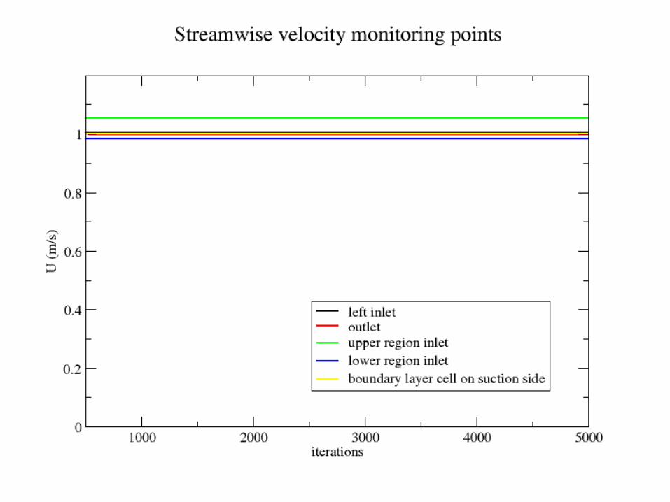
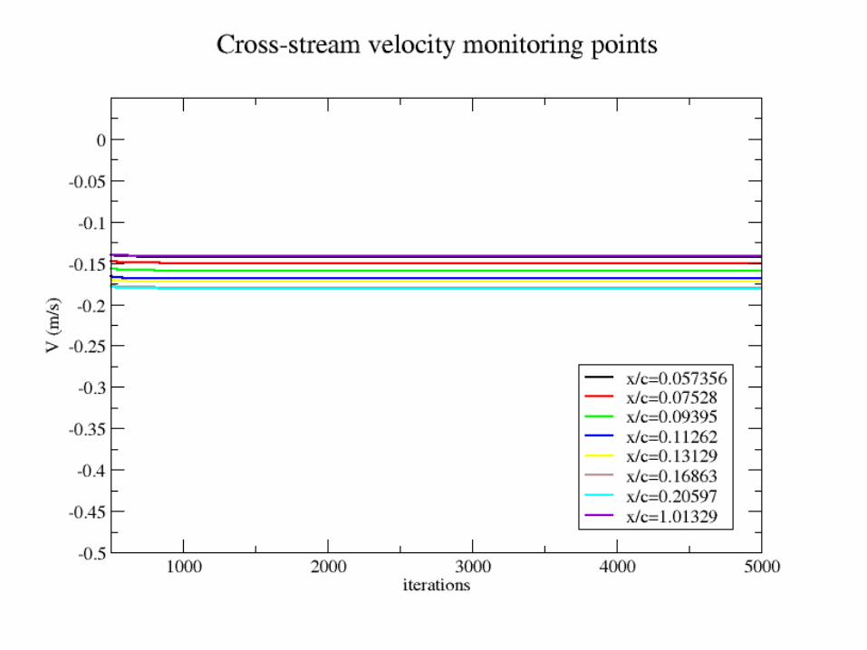
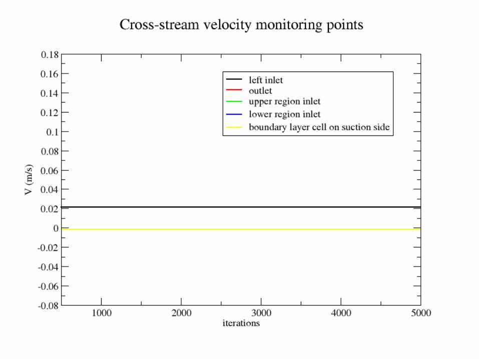
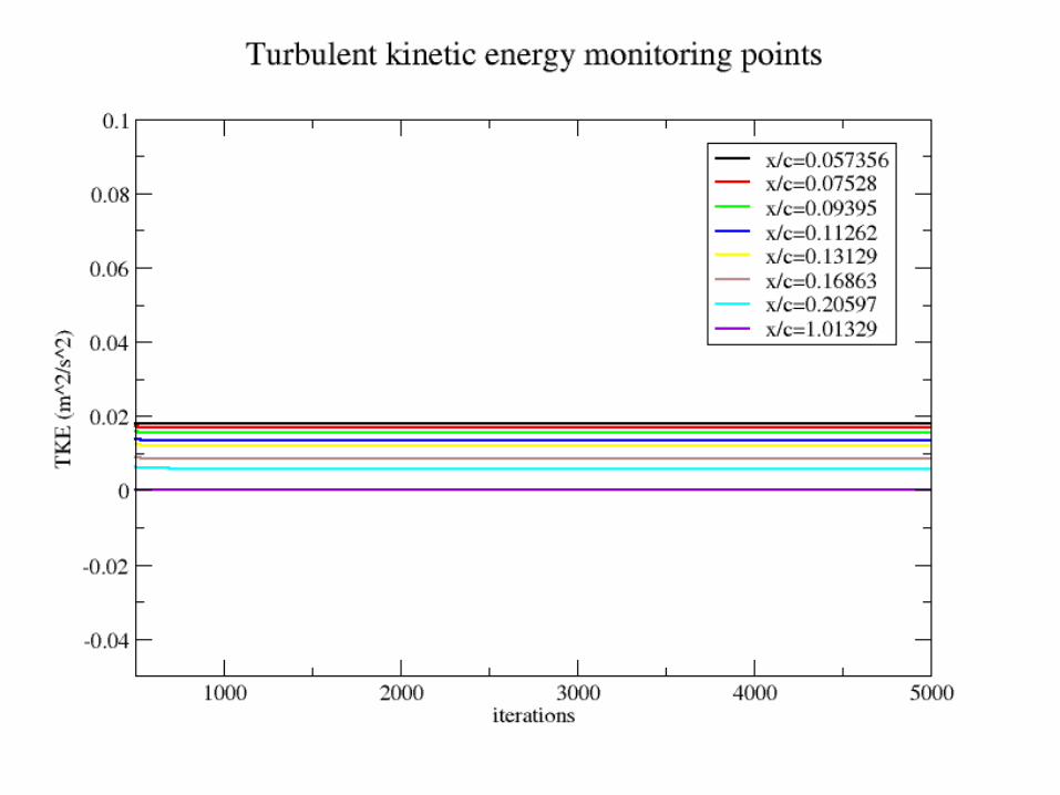
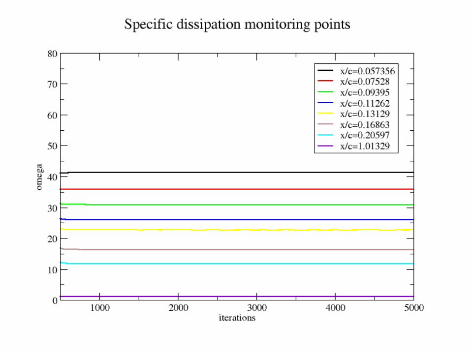
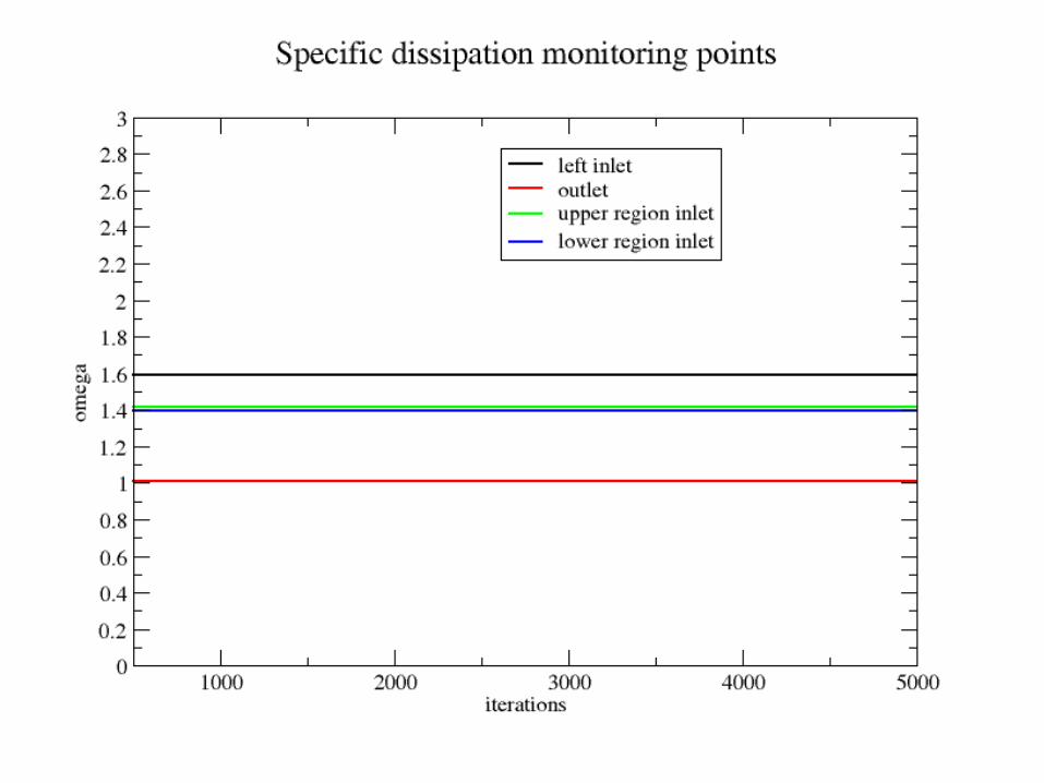
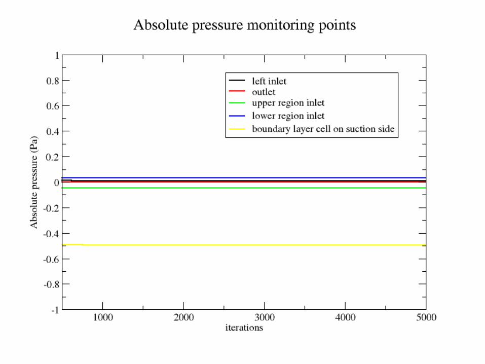
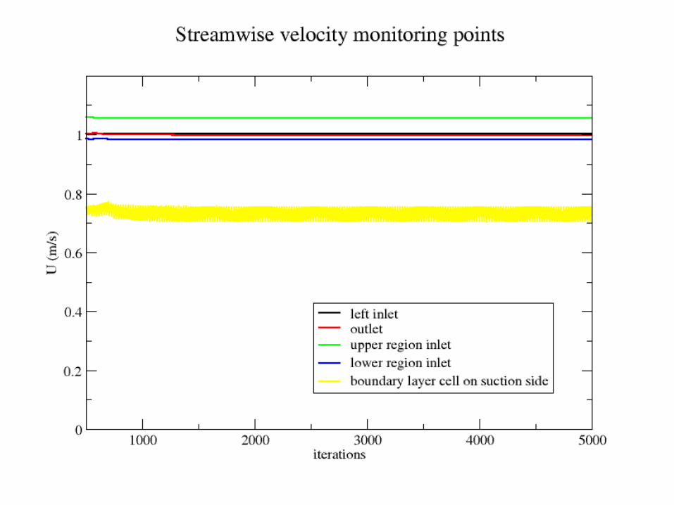
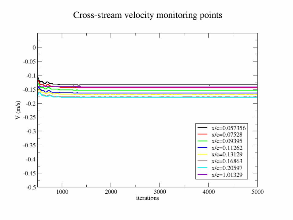
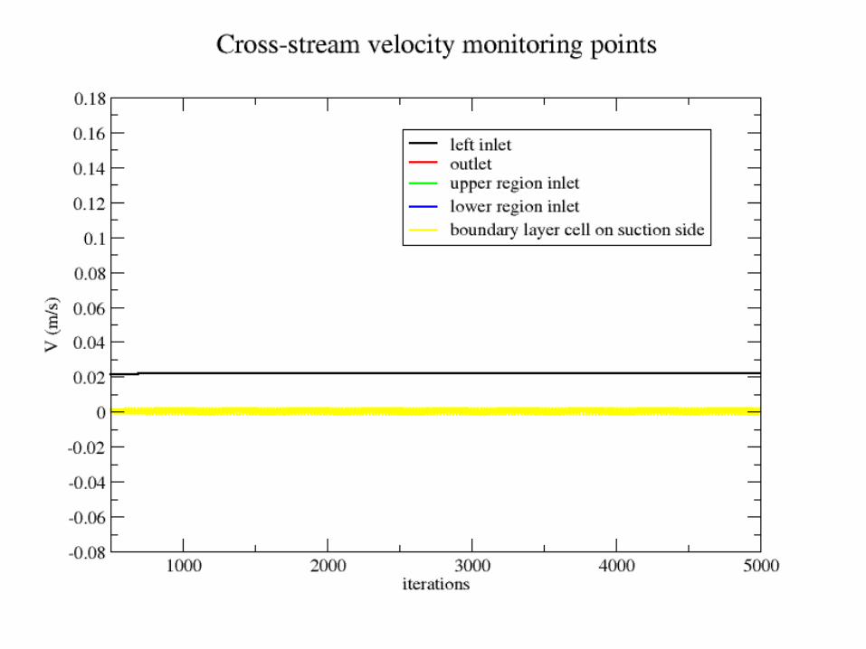
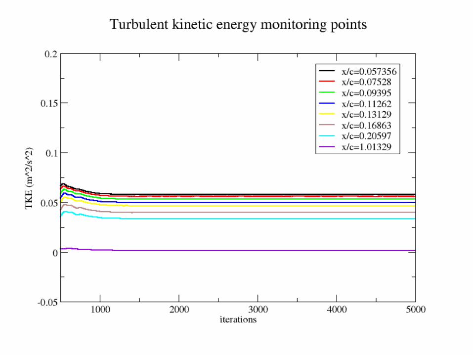
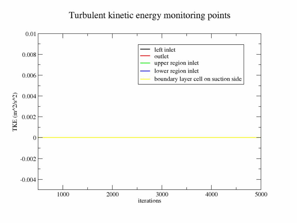
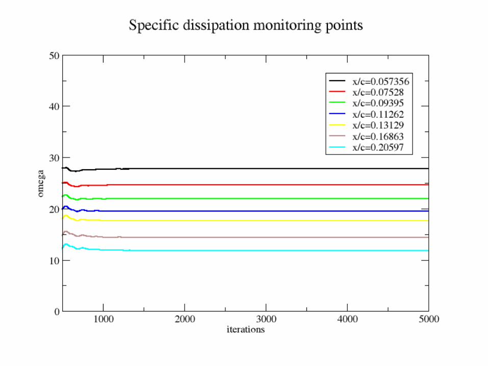
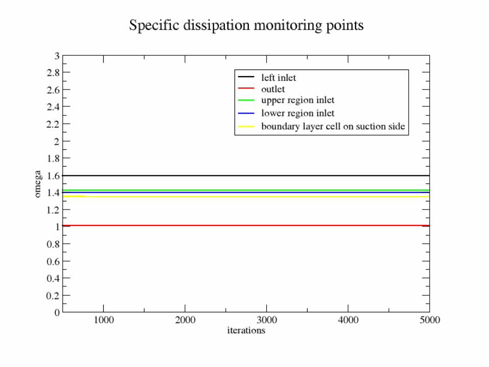
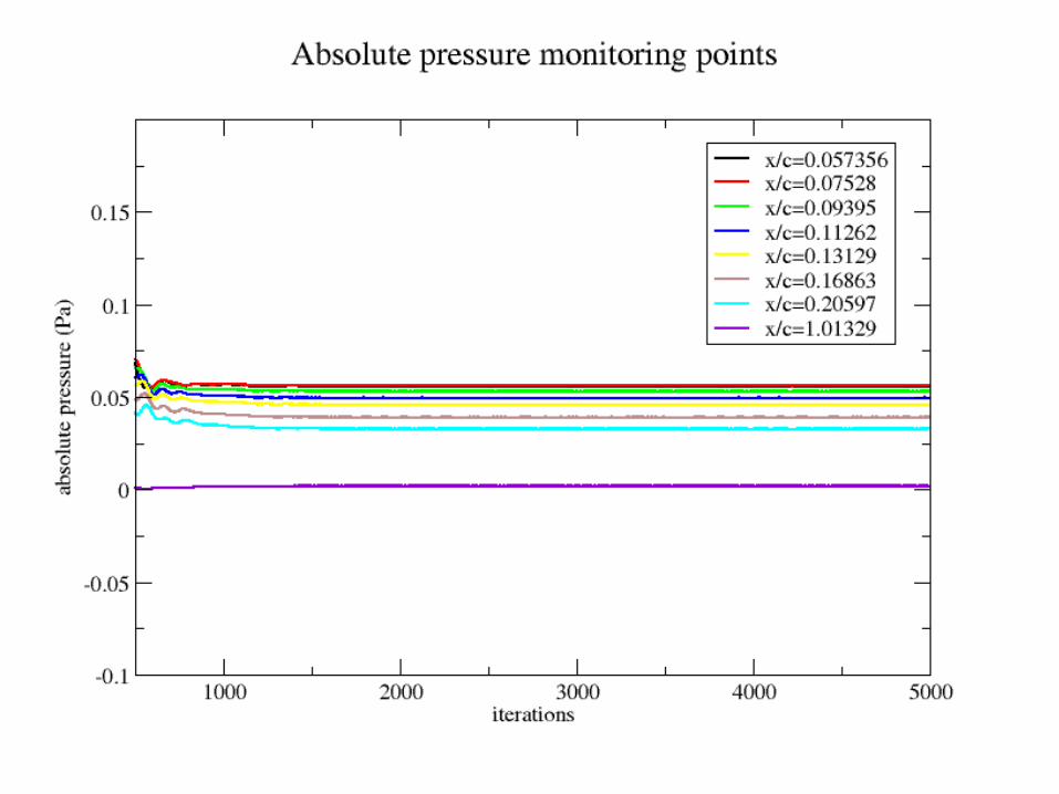
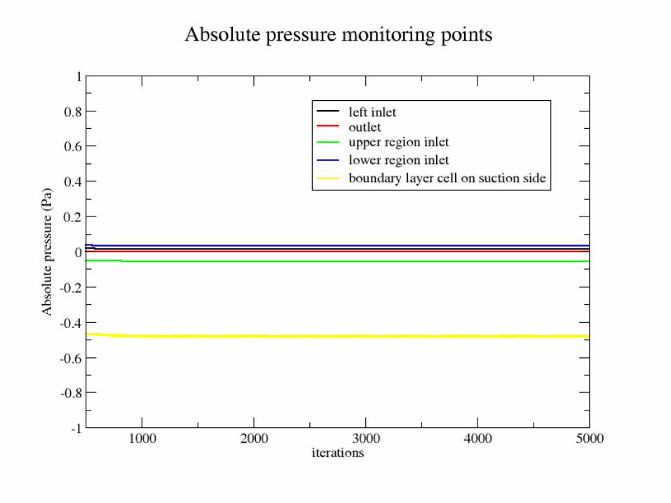
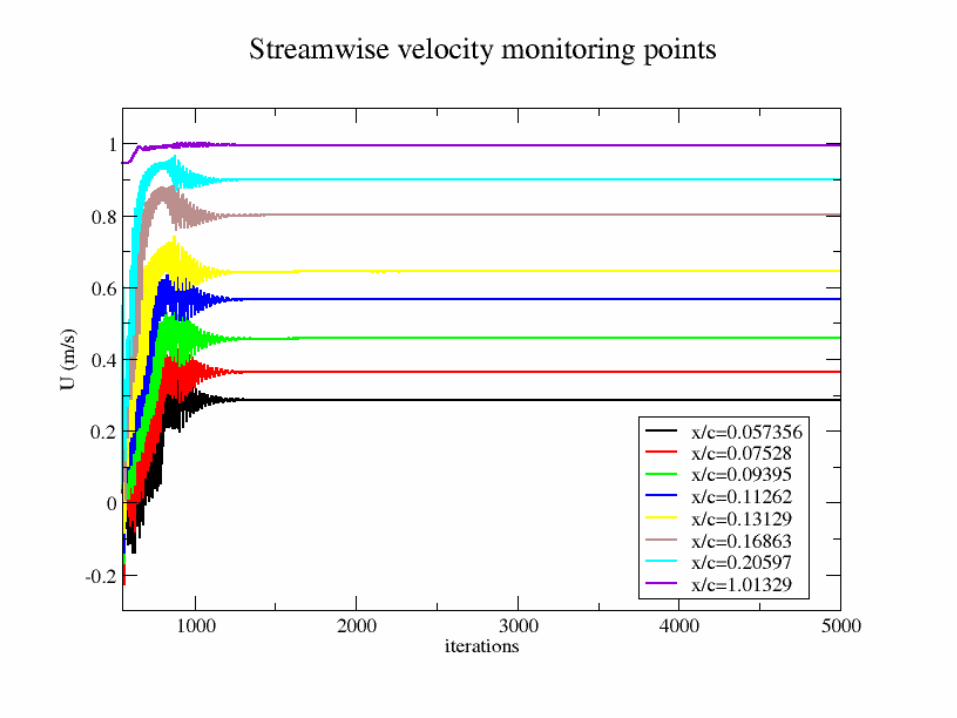
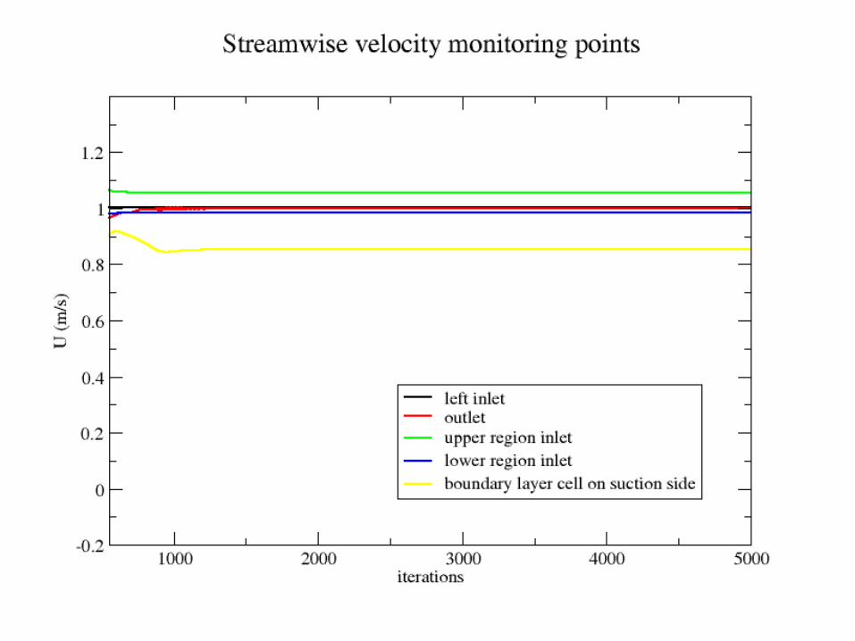
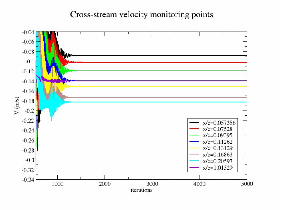
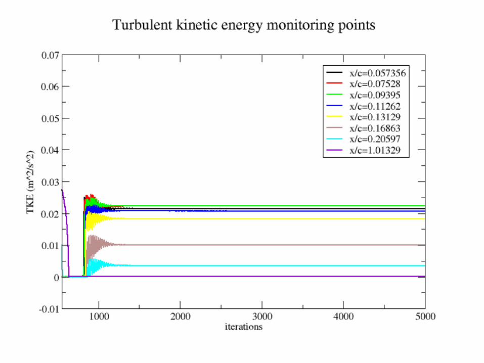
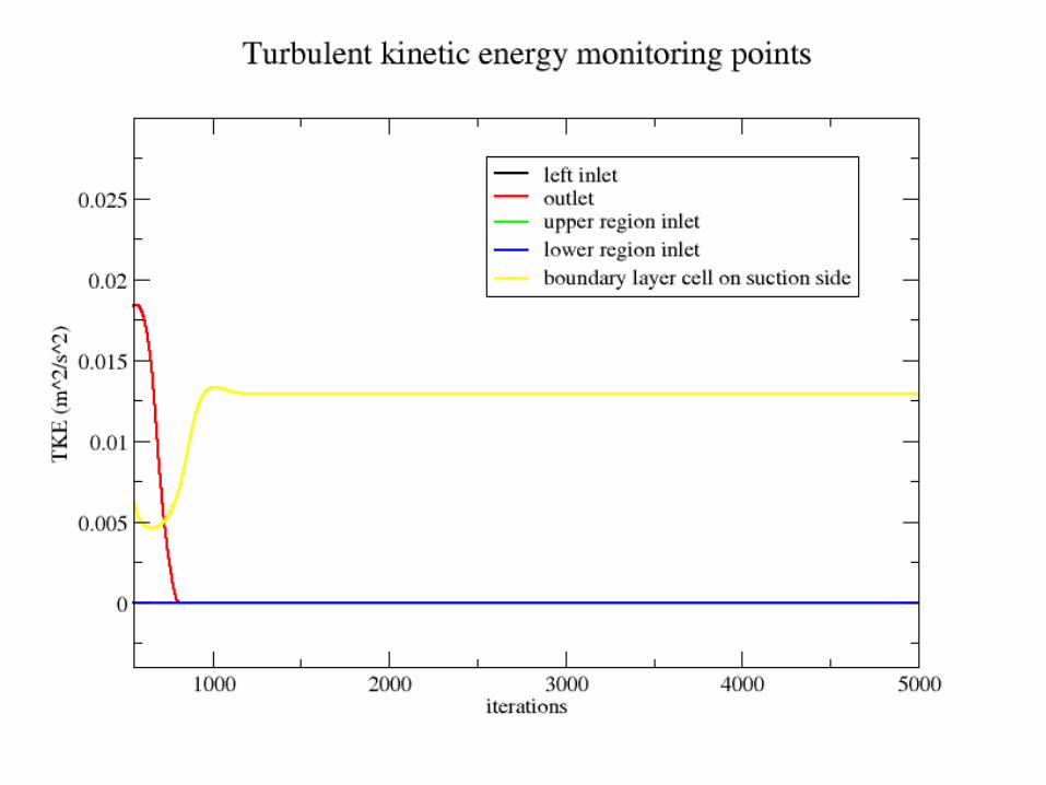
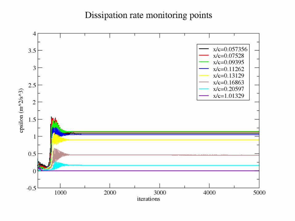
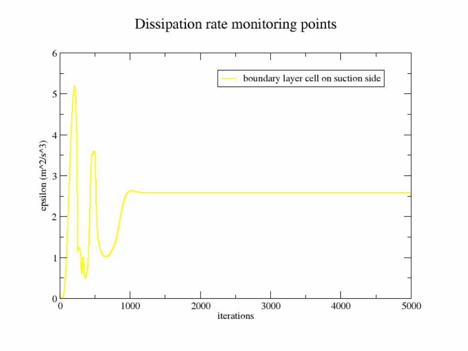
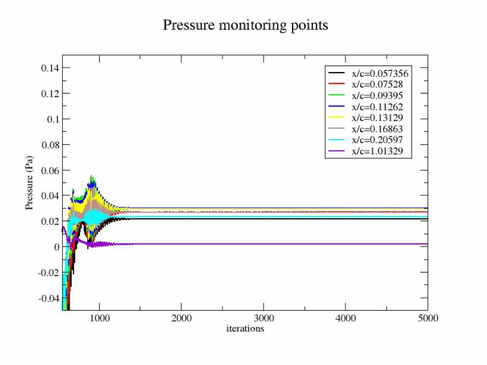
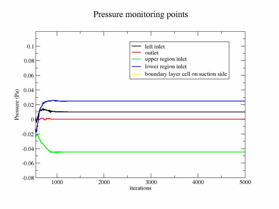
Monitoring points• The main variables in the models in the Code_Saturne
simulations (U-velocity, V-velocity, dissipation, pressure, turbulent kinetic energy and laminar kinetic energy - where applicable) are monitored at 13 points. There is a monitor at the 3 inlets and the outlet and one in the boundary layer of the aerofoil. The remaining 8 are at y=0 for the 8 x-values of the profiles.
• Residuals are shown in star-CD, however it was unable to converge using MARS with a blending factor of 0.5 and small under-relaxation factors .
• There was no information on convergence etc. For the provided v2-f results from Fluent.
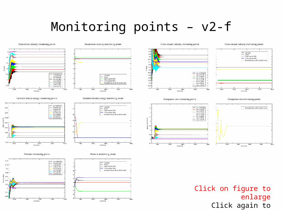
Monitoring points – v2-f
Click on figure to enlargeClick again to return
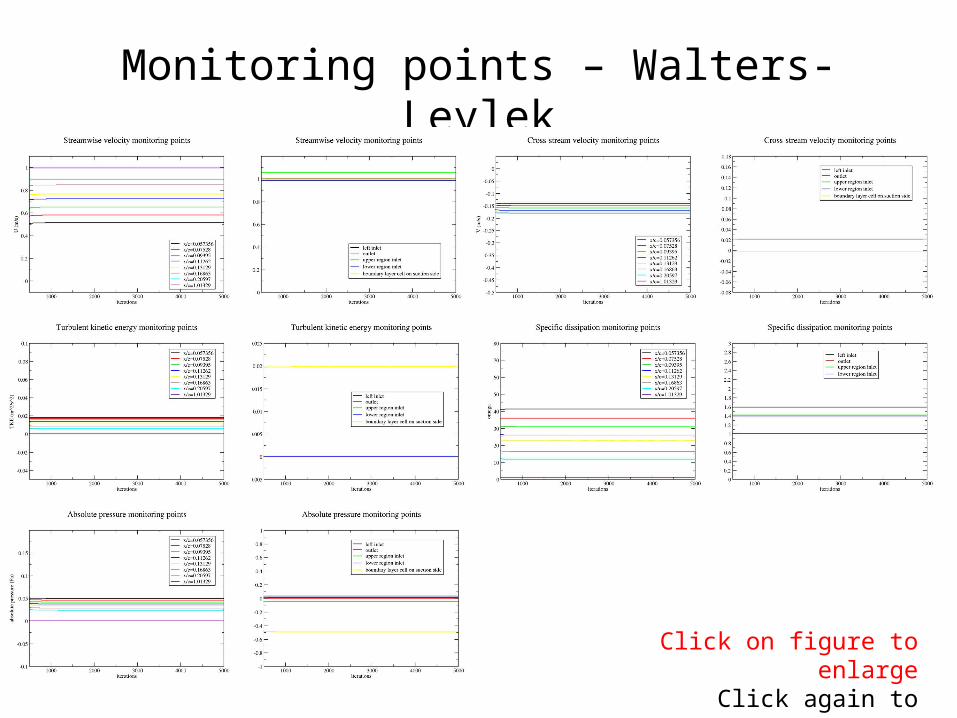
Monitoring points – Walters-Leylek
Click on figure to enlargeClick again to return
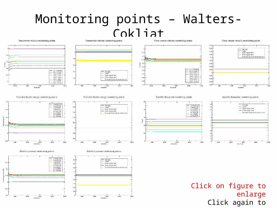
Monitoring points – Walters-Cokljat
Click on figure to enlargeClick again to return
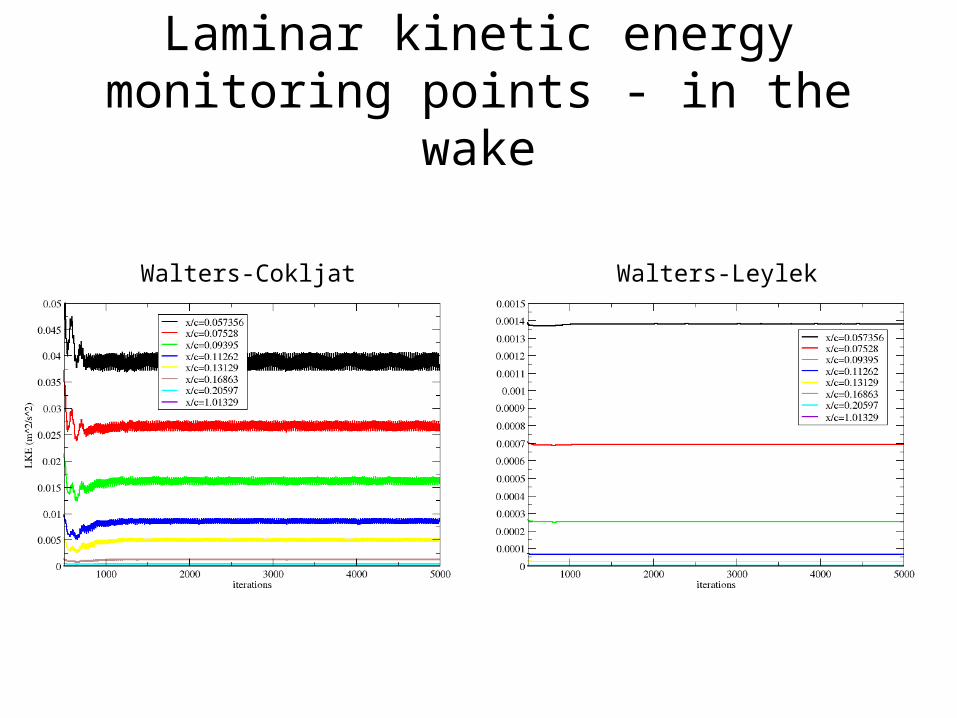
Laminar kinetic energy monitoring points - in the wake
Walters-Cokljat Walters-Leylek
Laminar kinetic energy monitoring points - in the wake
• Laminar kinetic energy is the result of energy from large length-scales being deflected from a wall. Therefore far away from the wall the values should be close to zero.
• The values predicted by the Walters-Cokljat model are far too high (of the order of 0.1 rather than 0.001).
• The values for kL become consistent very quickly for the Walters-Leylek model but the predictions continue to oscillate for the Walters-Cokljat model.
• The amplitude of the oscillations are very large close to the aerofoil but become smaller further down-stream.
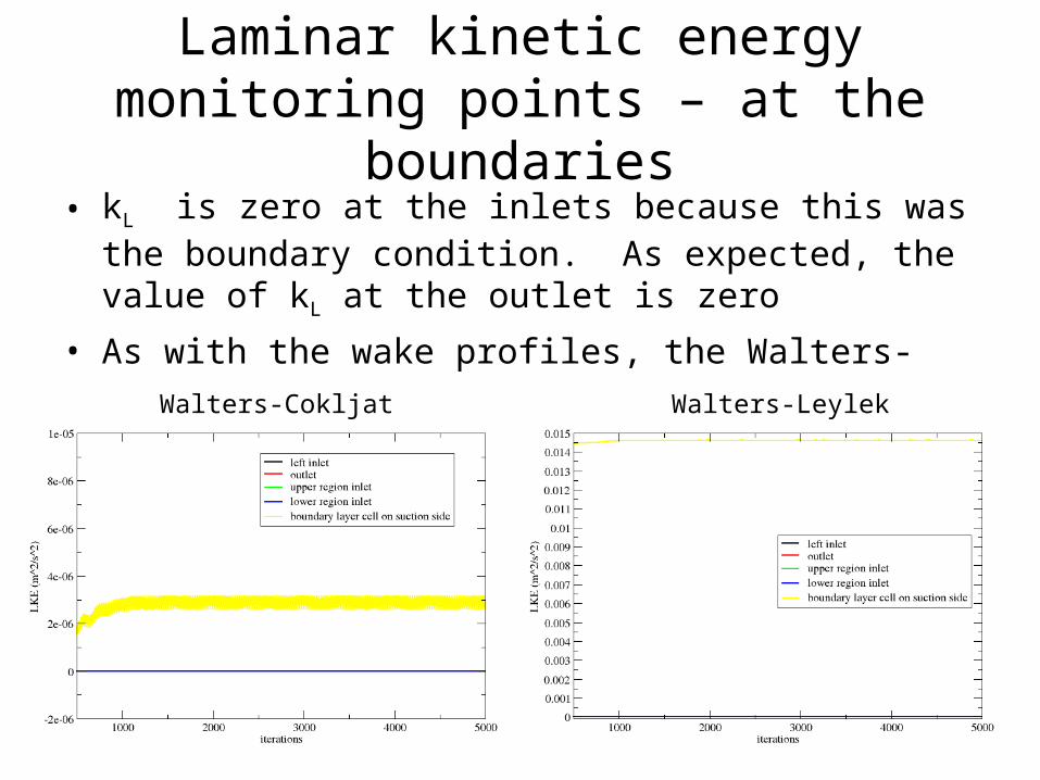
Laminar kinetic energy monitoring points – at the boundaries
• kL is zero at the inlets because this was the boundary condition. As expected, the value of kL at the outlet is zero
• As with the wake profiles, the Walters-Cokljat model does not give consistent values for non-zero laminar kinetic energy.
Walters-Cokljat Walters-Leylek
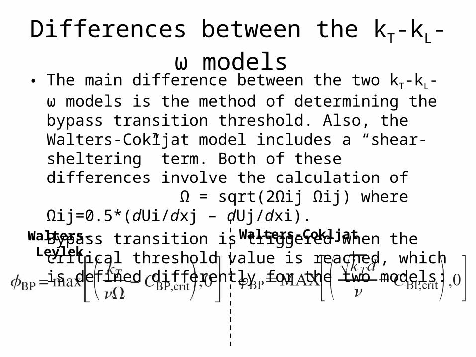
Differences between the kT-kL-ω models
Walters-Leylek Walters-Cokljat
• The main difference between the two kT-kL-ω models is the method of determining the bypass transition threshold. Also, the Walters-Cokljat model includes a “shear-sheltering” term. Both of these differences involve the calculation of Ω = sqrt(2Ωij Ωij) where Ωij=0.5*(dUi/dxj – dUj/dxi).
• Bypass transition is triggered when the critical threshold value is reached, which is defined differently for the two models:

Differences between the kT-kL-ω models • The calculation of bypass transition should not be an issue as
there is not sufficient disturbance in the free-stream to initiate bypass transition, however the shear-sheltering term does make a large difference to the production term in the turbulent kinetic energy equation.
where fW is the ratio of effective length-scale and turbulent length-scale; CSS is a constant.
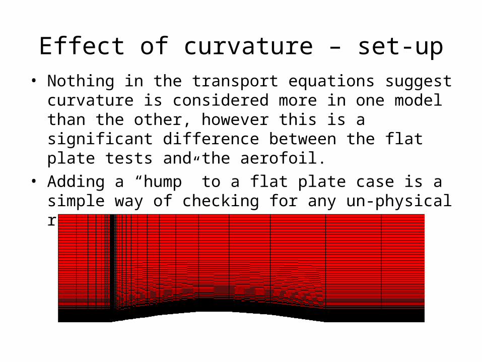
Effect of curvature – set-up• Nothing in the transport equations suggest curvature is
considered more in one model than the other, however this is a significant difference between the flat plate tests and the aerofoil.
• Adding a “hump” to a flat plate case is a simple way of checking for any un-physical results due to added curvature.
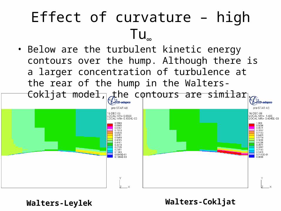
Effect of curvature – high Tu∞
Walters-Leylek Walters-Cokljat
• Below are the turbulent kinetic energy contours over the hump. Although there is a larger concentration of turbulence at the rear of the hump in the Walters-Cokljat model, the contours are similar.
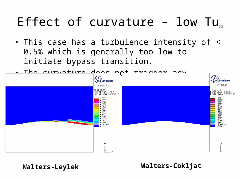
Effect of curvature – low Tu∞
• This case has a turbulence intensity of < 0.5% which is generally too low to initiate bypass transition.
• The curvature does not trigger any transition in the 2nd model.
Walters-Leylek Walters-Cokljat

Effect of curvature downstream – low Tu∞
• The Walters-Cokljat model predicts transition much further downstream, as is shown here.

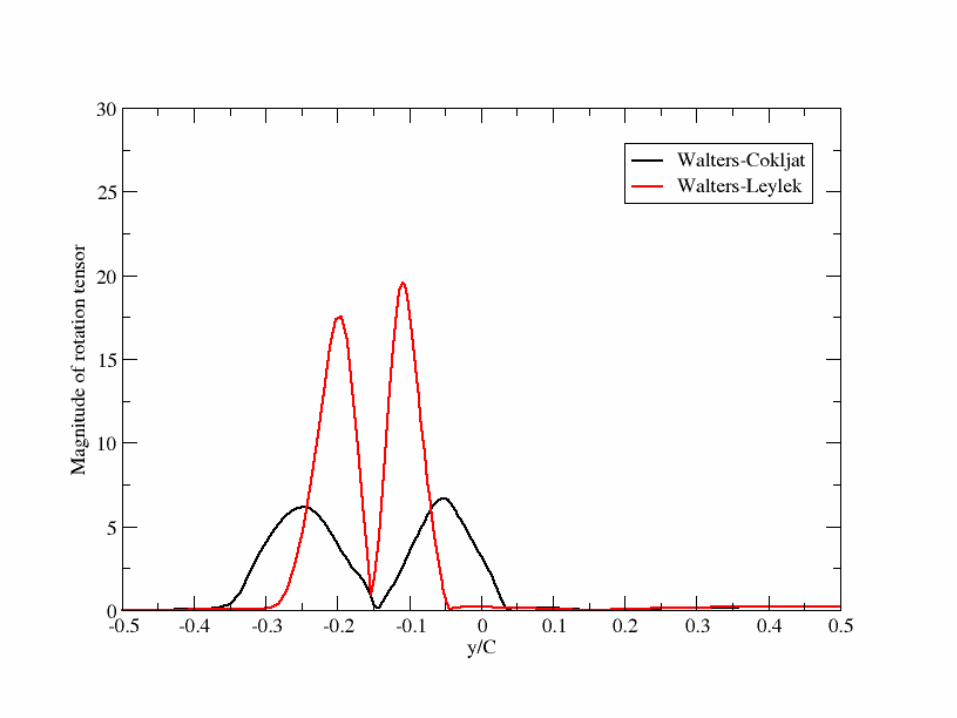
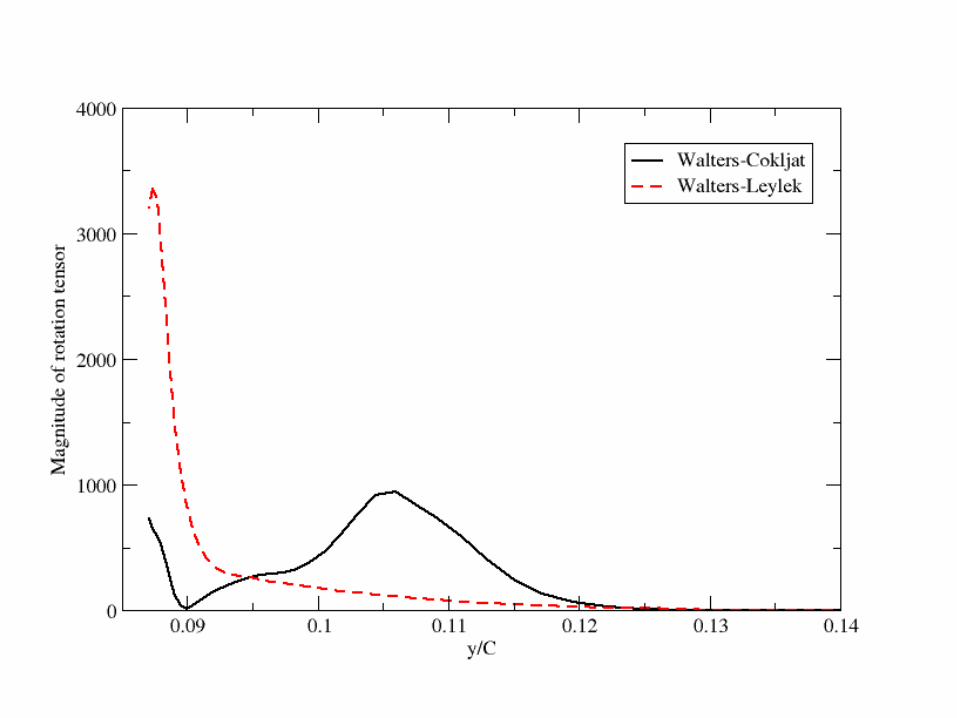
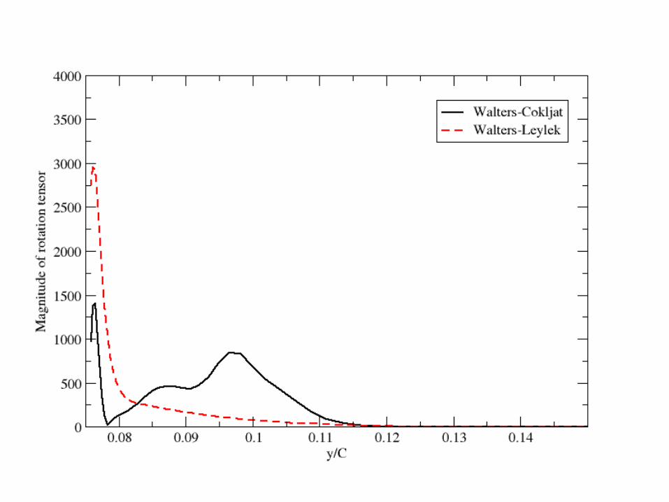
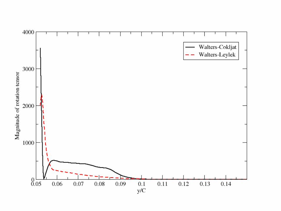
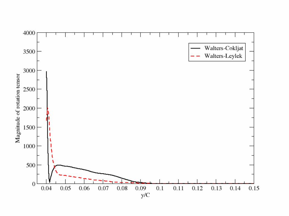
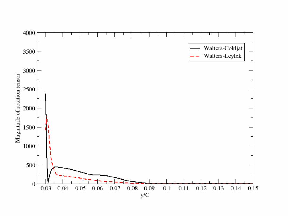
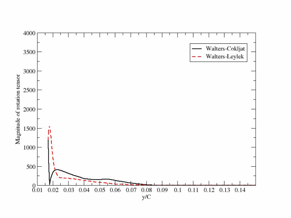
• There is no numerical data to compare these values of Ω to; however Ω should only be large very close to the wall
• Profiles at 10 equidistant points at the rear of the aerofoil show the Walters-Leylek model is qualitatively correct but the Walters-Cokljat implementation gives un-physical values.
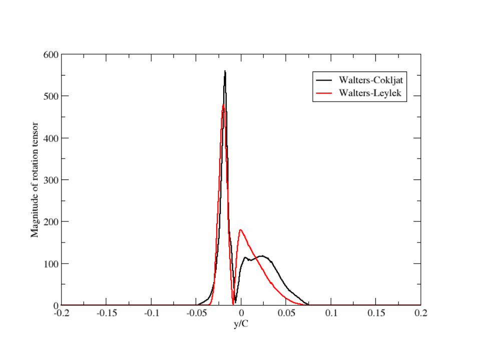
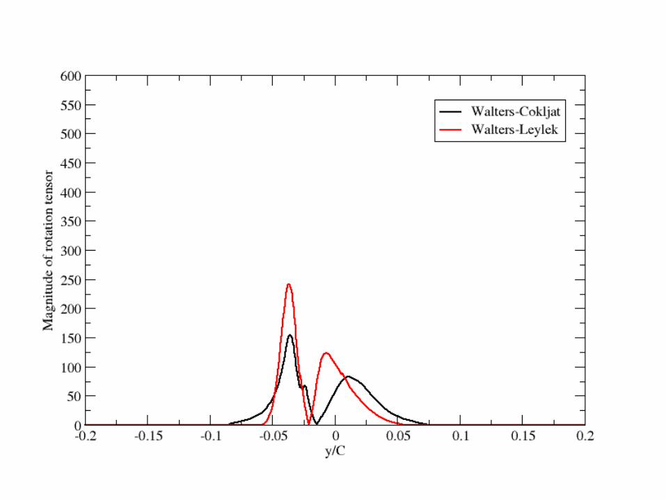
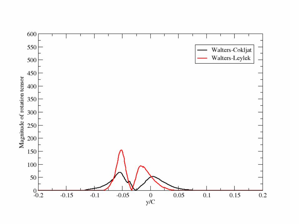
Profiles of Ω - over the aerofoil
Click on figure to enlargeClick again to return
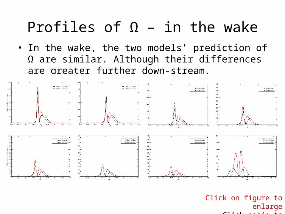
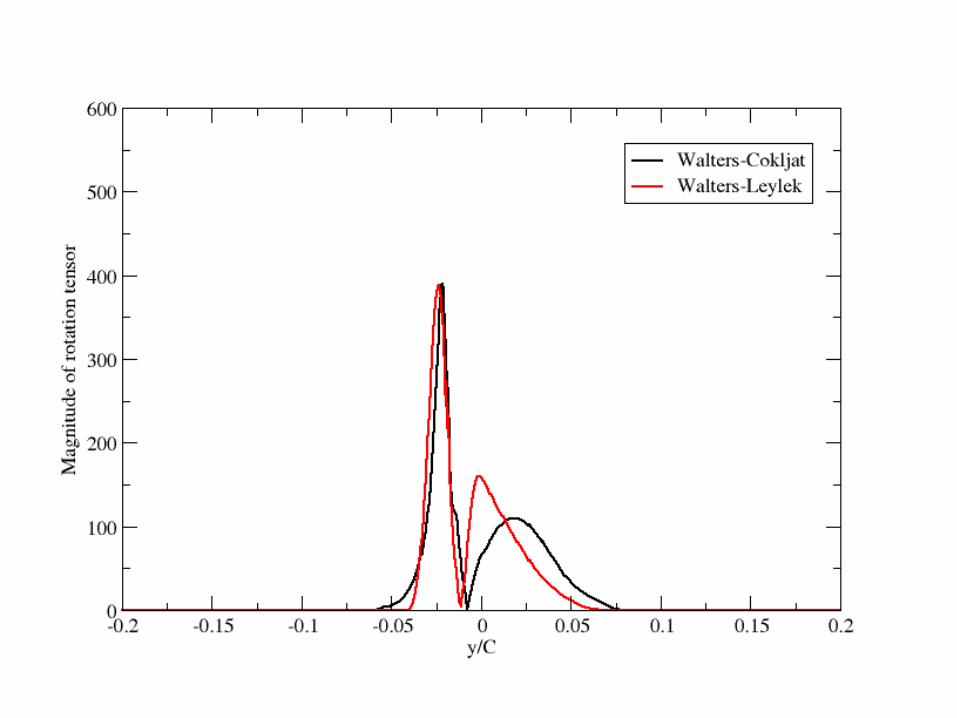
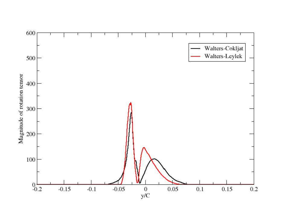
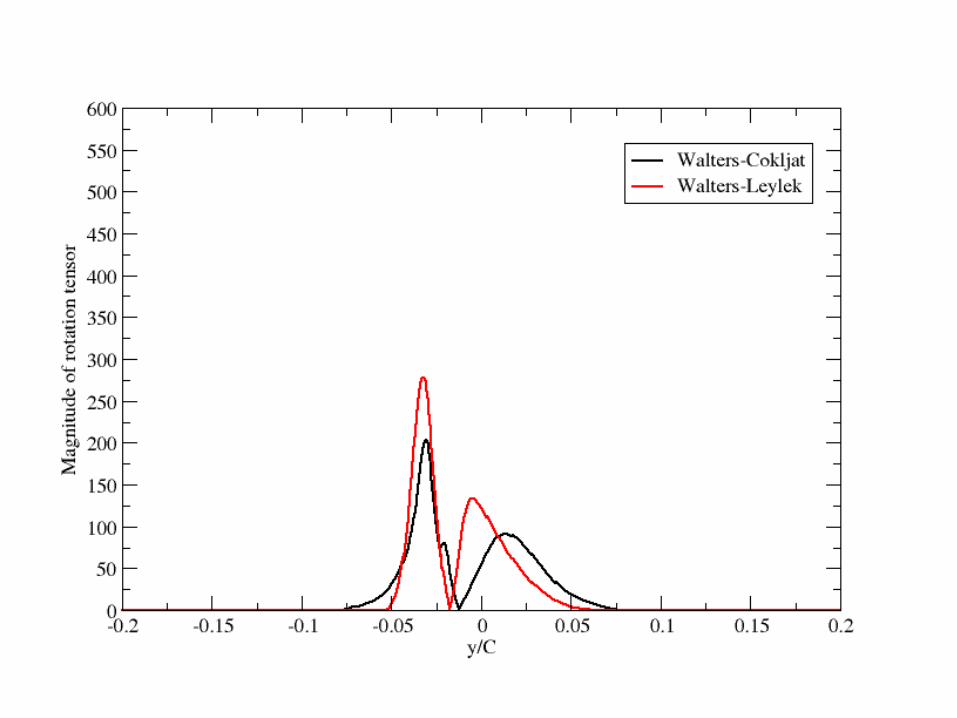
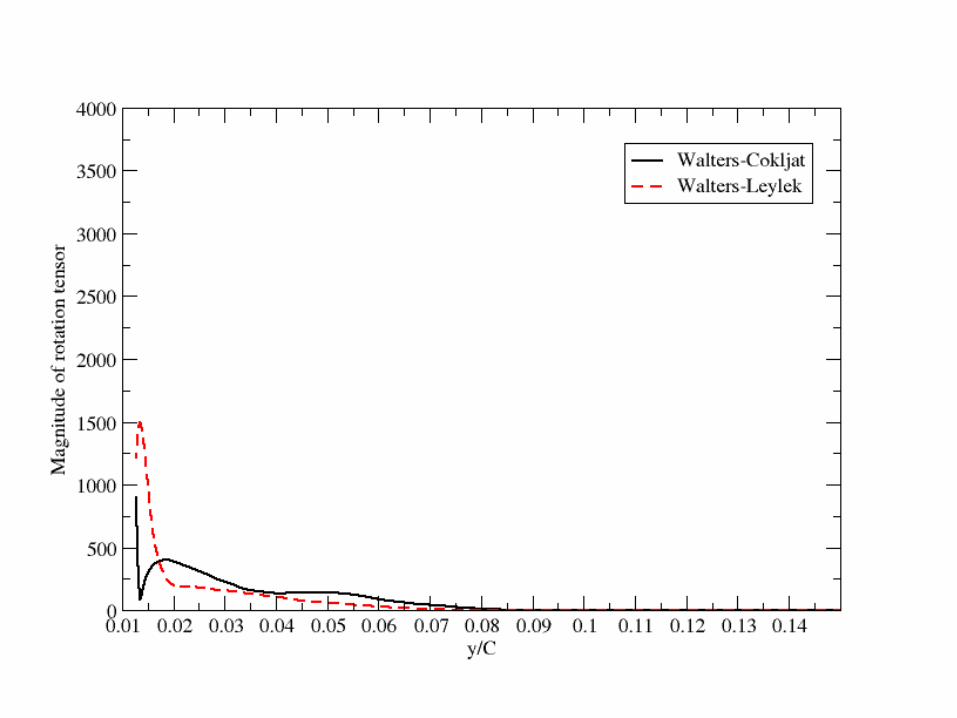
• In the wake, the two models’ prediction of Ω are similar. Although their differences are greater further down-stream.
Profiles of Ω – in the wake
Click on figure to enlargeClick again to return
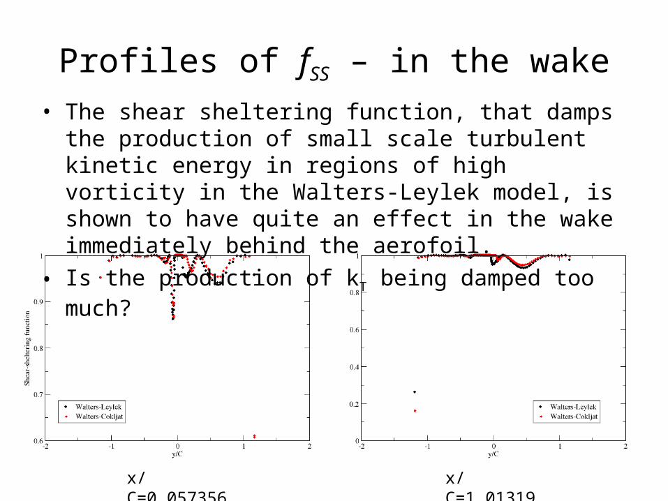
Profiles of fSS – in the wake• The shear sheltering function, that damps the production of
small scale turbulent kinetic energy in regions of high vorticity in the Walters-Leylek model, is shown to have quite an effect in the wake immediately behind the aerofoil.
• Is the production of kT being damped too much?
x/C=0.057356 x/C=1.01319
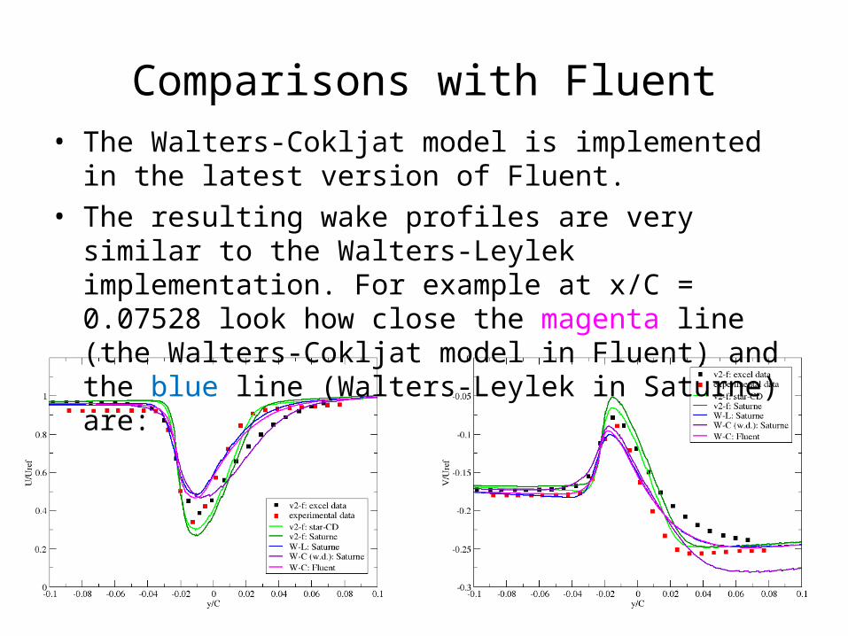
Comparisons with Fluent• The Walters-Cokljat model is implemented in the latest
version of Fluent.• The resulting wake profiles are very similar to the Walters-
Leylek implementation. For example at x/C = 0.07528 look how close the magenta line (the Walters-Cokljat model in Fluent) and the blue line (Walters-Leylek in Saturne) are:
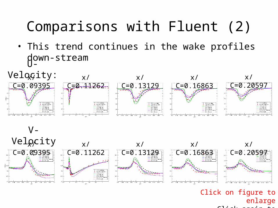
• This trend continues in the wake profiles down-stream
Comparisons with Fluent (2)
Click on figure to enlargeClick again to return
x/C=0.20597x/C=0.16863x/C=0.13129x/C=0.09395 x/C=0.11262
x/C=0.20597x/C=0.16863x/C=0.13129x/C=0.09395 x/C=0.11262
U-Velocity:
V-Velocity:
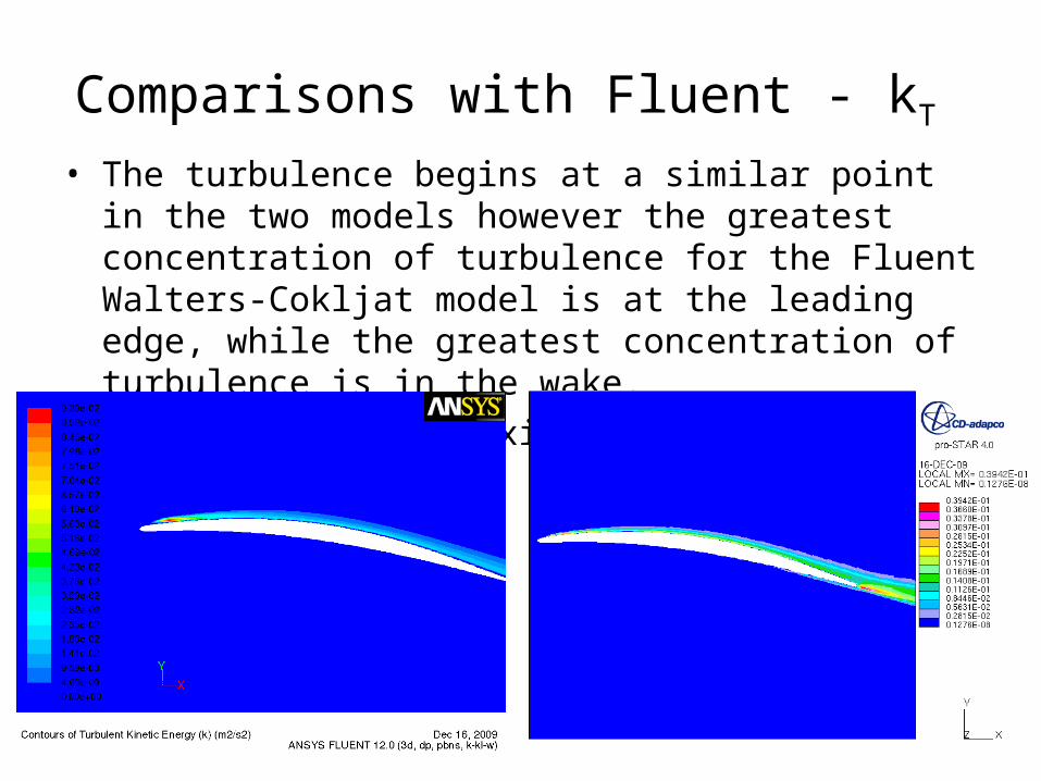
Comparisons with Fluent - kT • The turbulence begins at a similar point in the two models
however the greatest concentration of turbulence for the Fluent Walters-Cokljat model is at the leading edge, while the greatest concentration of turbulence is in the wake.
• Additionally the maximum values are very different.
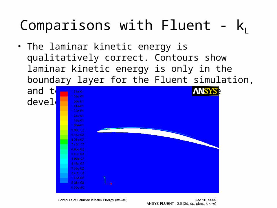
Comparisons with Fluent - kL • The laminar kinetic energy is qualitatively correct. Contours
show laminar kinetic energy is only in the boundary layer for the Fluent simulation, and tends to zero as the turbulence develops.
Conclusions: initial observations• The comparisons between the different codes and the
experimental results for the wake profile and pressure coefficient imply the set-up used in Code_Saturne is valid.
• Fluent and Star-CD show convergence is difficult to achieve; the residuals stop reducing after a normalised value of approximately 0.001.
• Despite this, all of the models, with the exception of the Walters-Cokljat model, give very good predictions of CP and good predictions of the wake profiles.
• The monitoring points in Code_Saturne show the variables keeping a consistent value after about 500 iterations, again with the exception of the Walters-Cokljat model.
Conclusions: further• The wake results from Fluent are very similar to those from
the Walters-Leylek run, which implies the problem lies only within the implementation of the Walters-Cokljat model.
• Curved surfaces appear to cause a large delay in transition with the Walters-Cokljat model when there is a low free-stream turbulence intensity.
• This could be associated with the calculation of the magnitude of the rotation tensor or its effect on the shear-sheltering term, fSS.
Current and further work• Data from the point of divergence in the Walters-Cokljat
model (43 iterations) is being examined closely to look for any particular triggers.
• A simple channel flow, with a known velocity profile, is being set up to check the Ω values calculated by the sub-routine.
• As curvature appears to affect the value of the shear sheltering function, an investigation is required to determine whether this is a weakness; if so, how to correct it.
• Since the point of transition is of importance, further analysis is being made on the contours of turbulence around the aerofoil for the different models (including comparisons in the same software)

END
The following slides are additional details and full size figures
The following slides are animations of the profiles as you progress
down the wake

Wake profiles – experimental results
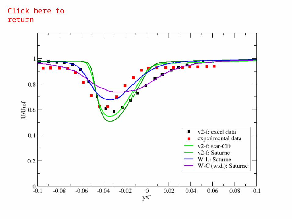
Wake profiles comparison:stream-wise velocity
Click here to return
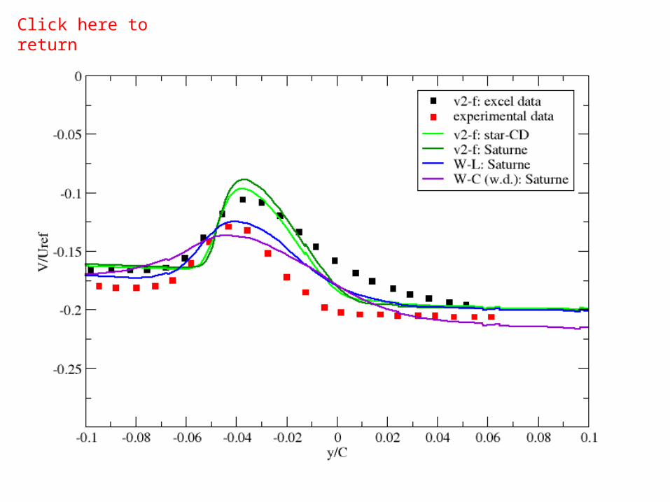
Wake profiles comparisoncross-stream velocity
Click here to return


The following slides are profiles with all important models


Wake profiles with just omega based models