Review of the magnetic measurement technique (experience of the SLC, LEP, CEBAF)

N.A.Morozov

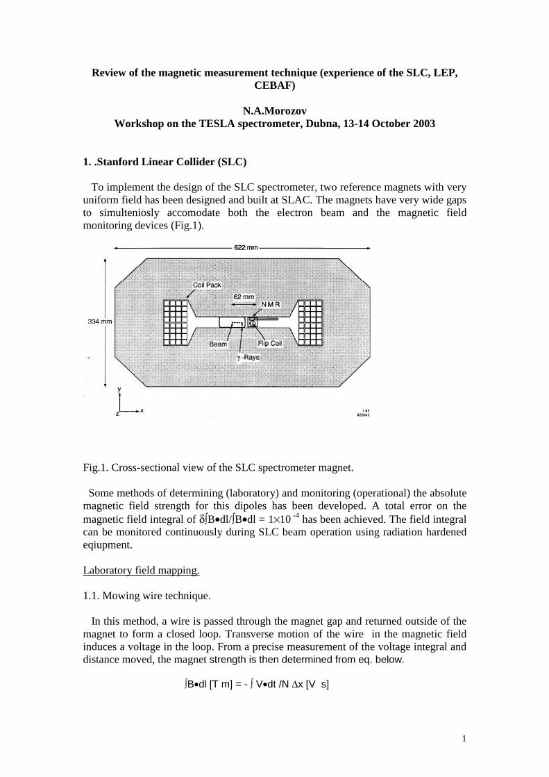
Workshop on the TESLA spectrometer, Dubna, 13-14 October 2003 1. .Stanford Linear Collider (SLC) To implement the design of the SLC spectrometer, two reference magnets with very uniform field has been designed and built at SLAC. The magnets have very wide gaps to simulteniosly accomodate both the electron beam and the magnetic field monitoring devices (Fig.1).

Fig.1. Cross-sectional view of the SLC spectrometer magnet. Some methods of determining (laboratory) and monitoring (operational) the absolute magnetic field strength for this dipoles has been developed. A total error on the magnetic field integral of δ�B•dl/�B•dl = 1×10 -4 has been achieved. The field integral can be monitored continuously during SLC beam operation using radiation hardened eqiupment. Laboratory field mapping. 1.1. Mowing wire technique. In this method, a wire is passed through the magnet gap and returned outside of the magnet to form a closed loop. Transverse motion of the wire in the magnetic field induces a voltage in the loop. From a precise measurement of the voltage integral and distance moved, the magnet strength is then determined from eq. below. �B•dl [T m] = - � V•dt /N ∆x [V s]

1

Here, �Vdt is the time integral of the induced voltage, N is the number of turns and ∆x is the distance moved in meters. The wires are secured in place at either end by wire holders at a tension of 1.5 Nt. The holders are mounted on precision traveling stages. The wire pack is aligned to be parallel to the long axis (z) of the magnet to an accuracy of 1 mrad. The loop is then completed outside of the magnet by a flexible cable. Both stages are aligned with the direction of travel parallel to the x-axis to a precision of 4 mrad, where the x-axis is perpendicular to both the z-axis and the magnetic field lines (the y-axis). This alignment error leads to an error on the field integral of 8 ppm. Both stages are mounted equidistant from the magnet center, 70.1 cm from the magnet end-plates. The y position of the stages can also be adjusted. These stages have 250 mm of travel and can be driven in l-µm steps at speeds up to 3 mm/sec. Stage positions are monitored by built in optical encoders which count lead screw rotations and are read through CAMAC. Roll, pitch and yaw are less than 0.02 mrad for this stage. The stage position accuracy is better than 30 ppm over the full range of travel. This is checked by mounting a laser retroreflector (corner cube prism) on the wire holder, setting up a laser interferometer system, and comparing the interferometer reading with that of the optical encoder. The interferometer has an absolute accuracy better than 1 ppm with automatic compensation for air temperature, pressure and humidity. In a measurement, both ends of the wire are moved simultaneously through a ramp up, steady speed and ramp down cycle to smoothly cover the distance desired (typically 10 mm). The actual speed affects the voltage induced but not the voltage integral, which depends only on the total distance moved. A system block diagram is shown in Fig.2.

Fig.2.System block diagram for “moving wire” technique. The voltage is read by an HP 3457A Digital Voltmeter (DVM). During measurements, the field from an NMR probe placed in a fixed position in the magnet and the magnet current are recorded. This corrects for drifts in the magnet current during a measurement and permits comparisons between measurements taken at different times. The mean standard deviation on all sets of ten measurements is

2

δ�B•dl/�B•dl = ±28 ppm. This is an indication of the short-term repeatability of this method, Estimated systematic errors for the “moving wire” method are summarized in Table 1. Table 1. Systematics errors for “moving wire” method. Error Source Error (ppm) Distance determination (stage) Misalignment of travel DVM accuracy Time base

30 8 25 2

Combined systematic error 40 1.2. Mowing probe technique. The second absolute measurement technique, “moving probe,” measures the field integral by driving an NMR probe and a Hall probe along the length of the magnet in small steps. In this manner the magnet strength is determined by summing over the measurements of the magnet using the trapezoid rule �B•dl = Σ[(Bi + Bi-1)/2]dli. The Bi are the field measurements at each point and dli is the step size. The probes are mounted with a laser retroreflector on a rail assembly which runs through the magnet and uses the laser interferometer to measure the probe position. The NMR probes are custom made, radiation hardened, miniature probes (MetroLab Model 1065) attached to the probe electronics by a flexible shielded cable. Absolute accuracy for the NMR system is 10 ppm. The Hall effect probe is used in the fringe field of the magnet. This probe has a precision of 300 ppm and is calibrated during measurements by the NMR system in the region where both operate. Unlike the NMR probe, the Hall probe is sensitive to rotations. The maximum possible tilt (40 mrad), given the rigidity of the probe holder, would result in an error of 800 ppm. However, the Hall probe only measures 6% of the total field integral so the maximum expected contribution to the error is 48 ppm. A schematic diagram of the mapping system is shown in Fig.3.

Fig.3.System block diagram for “moving probe” technique.

3

The short-term repeatability of this method is quite good (δ�B•dl/�B•dl = 15 ppm). Table 2 summarizes the estimated systematic errors with this technique. Table 2. Systematics errors for “moving probe” method. Error Source Error (ppm) Position determination (laser) Misalignment of laser to beam path NMR system Hall probe precision (300ppm×6%) Hall probe tilt (800ppm×6%) Linear interpolation

1 0 10 18 48 10

Combined systematic error 53 Field monitoring techniques The absolute measurements are used to simultaneously calibrate two independent, transferable standards for monitoring the field strength: (1) a rotating “flip coil,” (2) three stationary NMR probes. These methods allow the field integral to be monitored while the magnet is installed in the beam line. 1.3. Flip coil. The flip coil consists of a rod of used silica quartz 2.80 m long and 15 mm in diameter (see Fig.4). An AC synchronous motor rotates the coil at 3 rpm and the entire assembly is inserted in the magnet gap. The voltage induced by the changing flux is connected by a brush and slip ring assembly to the DVM system. Four flip coils were built to insure that spares exist. The time integral of the voltage (�B•dl) over a half-wave-form will be proportional to the magnet strength according to the relationship: �B•dl [Tm] = - � V•dt [V s] / N (2d), where d is the effective diameter of the coil and N is the number of turns in the coil. The flip coil is expected to be insensitive to temperature changes. Each flip coil is calibrated in each magnet at six magnet excitations using both the “moving wire” and “moving probe” standards. In the final calibration, the “moving wire” data is used because of the better fit and better absolute accuracy. In Table 3, the estimated systematic errors with the flip coils are shown, excluding absolute calibration error. The dominant error for this method is the accuracy of the DVM (35 ppm) in measuring the induced voltages. A typical 1 mrad misalignment of the flip coil would contribute 1 ppm to the measurement error. The error contributed by the uncertainty on CT for a 15 oC temperature rise is 9 ppm. Short-term repeatability is measured to be σ = 28 ppm.

4

Fig.4. Drawing of flip coil showing quartz rod, coil pack, support stucture, and driver system. Table 3. Systematics errors for “flip coil” method. Error Source Error (ppm) DVM accuracy Time base Misalignment of flip coil Average fit error Thermal effects

35 2 1 20 9

Combined systematic error 42 1.4. NMR probes. The second monitoring method uses the readings from a set of three NMR probes installed in the flip coil support structure. These probes are located at the center of the magnet and 50 cm from either end. Due to the limited space available, the probes are custom manufactured, miniature MetroLab probes as described previously. Accurate measurements at specific points are possible with this technique, but not a direct measurement of �Bdl. The field integral must be inferred from a cross-calibration. Therefore, this technique is sensitive to magnet saturation effects and thermally induced geometry changes. Calibration of the NMR probes is similar to the flip coils but with “moving wire” data taken at 40 different excitations from 1000 to 600 amps because of the expected sensitivity to saturation effects a third-order fit. The mean fit residual here is 42 ppm when fit to the “moving wire” measurements. Systematic errors for the NMR probes include the NMR system accuracy (10 ppm) and a typical l-mm uncertainty in probe position (20 ppm). The average fit error is 42 ppm. The NMR probes have a much larger thermal coefficient (CT = 12.5±2 ppm/ oC) than the flip coils due to the expansion coefficient of steel and the error in this results in a 30 ppm error on �Bdl for a 15 oC temperature rise. Estimates of this error come from the

5

variations in multiple measurements of CT. These errors are summarized in Table 4. Short-term repeatability with this method is measured to be 5 ppm. Table 4. Systematics errors for NMR probes. Error Source Error (ppm) NMR system Probe position Average fit error Thermal effects

10 20 42 30

Combined systematic error 42 1.5. Conclusion. Table 5 summarizes the known contributions to errors in the measurement of the field integral for each monitoring method. The relative error is the systematic error for each monitoring technique, determined previously. Adding all these errors in quadrature yields the combined error. The mean error is defined here as mean difference between the flip coil measurement and the other methods for a series of measurements taken at various magnet excitations. The monitoring methods have been calibrated with the absolute standards. Combining all sources of errors results in a total error on the measurement of the field integral, by the best monitor, of 100 ppm. This includes all known systematic errors and the measurement precision. Table 5. Summary of errors in monitoring of �B dl. Error Source Flip coil

(ppm) NMR (ppm)

Absolute Uniformity Survey Relative

72 54 4 42

72 54 4 57

Combined 100 110 Precision (short-term) 28 5 2. The ARC project (CEBAF). The ARC is an equipment of CEBAF (at Jefferson Lab) to measure the absolute energy of the electron beam. The determination of the beam energy is done throw a very accurate measurement of the field integral of a reference dipole, electrically connected in series with the bending magnets transporting the beam from the accelerator to the experimental hall. A new method is used to determine the field integral. Finally, the goal to reach an accuracy of a few 10 –5 on the field integral has been reached. The principal view of the experimental arrangement is in the Fig.5.

6

2.1. Field integral measuring device. The field integral measuring device uses an original technique. It makes use of the well known ‘translating coil’ technuque, where the flux changes through a small coil are recorded while the coil travels inside the gap along the beam path. But here it was used the special arrangement of two coils accurately spaced at a distance about the magnetic length of the reference magnet, and connected in series. This design results in a ‘zero-measurement’ giving an unprecendented accuracy in terms of field integral measurement. Assuming that the first coil final position is close to the second initial position, that the field is zero at the first coil initial position and at the second coil final position, and that both measuring coils have the same area, one can show that:

� ��+

−−=)(

)(

*)*()(xt

At

LB

A

B

A

SLBoBdzdttVdx

where • A and B are the departure and arrival points of the first moving coil; • A+L=B and B+L the corresponding points of the second moving coil; • V is the output voltage of the two coils in series; • Bo is the central field at point B; • L is the distance between the axis of the two coils; • S is the average magnetic area of the two coils. This equation shows that the double integral measurement consists of the difference between the true and assumed field integral; it is small compared to the field integral itself. In this measuring method, there are only two parameters to be measured with an accuracy of about 10 –5 : • The distance L between the mechanical axis of the two coils; • The central field Bo for each measurement.

7

Fig.5. Principle of the measurement. 2.2. The experimental apparatus. A. The search coils. To avoid second oder effects and to provide a consistency check in the comparison between forward and backward data, the two coils must be indentical in terms of magnetic area within a relative accuracy of few 10 –5. Several sets of search coils where calibrated and then balanced using a rotating device inserted in a homogeneous dipolar field. By carefully adjusting the number of turnes of the coils, it was possible to minmize the residual area between two coils to less then ±15 ppm. A special attention was given to the measurement of the distance between the mechnical axis of the search coils after mounting. This was done with accuracy ±7 ppm and with fitting by the temperature dependence. B. The NMR probes. A set of four NMR probes (MetroLab) was used to measure the central field field from 0.043 to 1.06 T, with accuracy of 2 ppm. C. The mechanical part. The mechanical parts of the system consists mainly of: • The reference dipole support; • The 6 m long measuring system support; • The moving measuring system, consisting of a 3 m long composite board on

which the four NMR probes and two search coils are mounted;

8

• A 3 m linear encoder to measure the coil position with an accuracy of about 100 µm an a resolution of 2.5 µm;

• Two µ-metal magnetic shield. D. The hardware. The integral measurement sequence is fully automatic. It consists of the following phases: • Linear encoder initialization; • Measure of the central field by NMR; • Forward pass flux integration; • Backward pass flux integration; • Check of the central field by NMR. In addition to this measurements, 4 probe temperatures and the current in the dipole are recorded at the beginning and at the end of the sequence. 3. LEP spectrometer magnet. For the determination of the LEP spectrometer magnet integral field two measurement systems have been set up. The first for a long mapping campaign in the laboratory, to scan all the accessible parameters of the magnet. The main components of this test bench were NMR probes, Hall plates and an electronic ruler to allow the length measurements. The NMR probe for the central field monitoring and the Hall plate for the fringe field were mounted on a carbon arm which was sliding on a marble bench. The ruler was fixed on the same marble bench and a sensor was sliding with the measurement arm. This system is not transportable and does not allow measurements inside the vacuum chamber. In order to check the total integral value inside the vacuum chamber and, even more important, to investigate the magnetic field after the magnet transportation from the laboratory to the LEP tunnel, a second measurement system was designed and commissioned. This system also uses NMR probes for the central region of the core, and a searching coil for the end field regions. Both instruments are mounted on a small wagon (mapping mole), which is moving inside the beam pipe. The mole is pulled by a toothed belt driven by a stepping motor. The field monitors locations are measured by a laser interferometer, through a retroreflector installed on the mole. The fringe field is evaluated integrating the voltage induced on the searching coil while moving in the end regions. 3.1. Test bench. The measurement system was set up initially in the laboratory located at ground level in the former ISR accelerator tunnel, where some equipment was already installed for previous experiments on a normal iron-concrete LEP bending magnet, and the spectrometer dipole was placed for the mapping campaign before the transportation in the LEP tunnel. In Fig.6 the test bench layout is displayed. The test bench sketched in Fig.7 consists of a marble bench with an optical ruler. The field is measured by an NMR probe and two Hall probes which are mounted on a carbon fibre

9

arm on a translation stage. The mechanics are optimised for position reproducibility (2 µm) and stability with respect to temperature variations. In this setup the end field region is measured with the Hall probes, which allow field measurements down to the µT level. The relative accuracy of the Hall probes is only 4×10 -4. Therefore the central field region was measured by more accurate NMR probes.

Fig.6. Test bench layout.

Fig.7. The mapping bench which allowed a determination of the integrated magnetic field of the magnet in the laboratory.

10

3.2. Mapping mole. The chariot has been constructed with non-magnetic materials. Four bronze-beryllium springs are inserted in the upper wheels support, in order to keep the trolley stably pushed against the vacuum pipe walls. The vacuum chamber in the spectrometer magnet is lifted up of 2 mm from the center of the dipole yoke, in order to guarantee enough space between the lower pole tip and the beam pipe for the four fixed NMR probes. The alignment was carefully studied and the geometry was designed to put the NMR probes and the searching coil in the center of the dipole gap, making them slide along the ideal beam trajectory. A schematic diagram of the mole is shown in Fig.8.

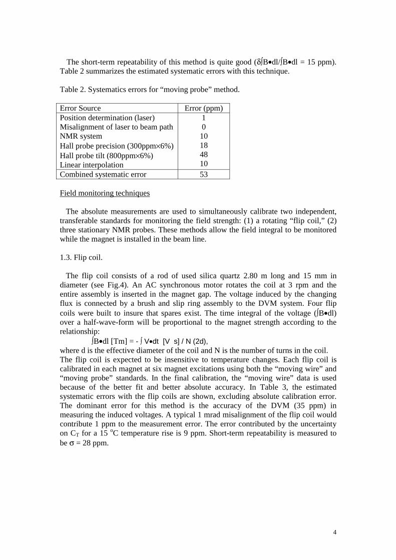
Fig.8. Schematic diagram of the mapping mole. 3.3. Position monitoring with interferometer. An accurate position monitoring is needed to evaluate the total integral field. For this purpose a laser source was adopted in order to perform a linear interferometer distance measurement. The diagram of the system is shown in Fig.9. This equipment gives a relative error of 5×10 –7 for the mole position determination.

11

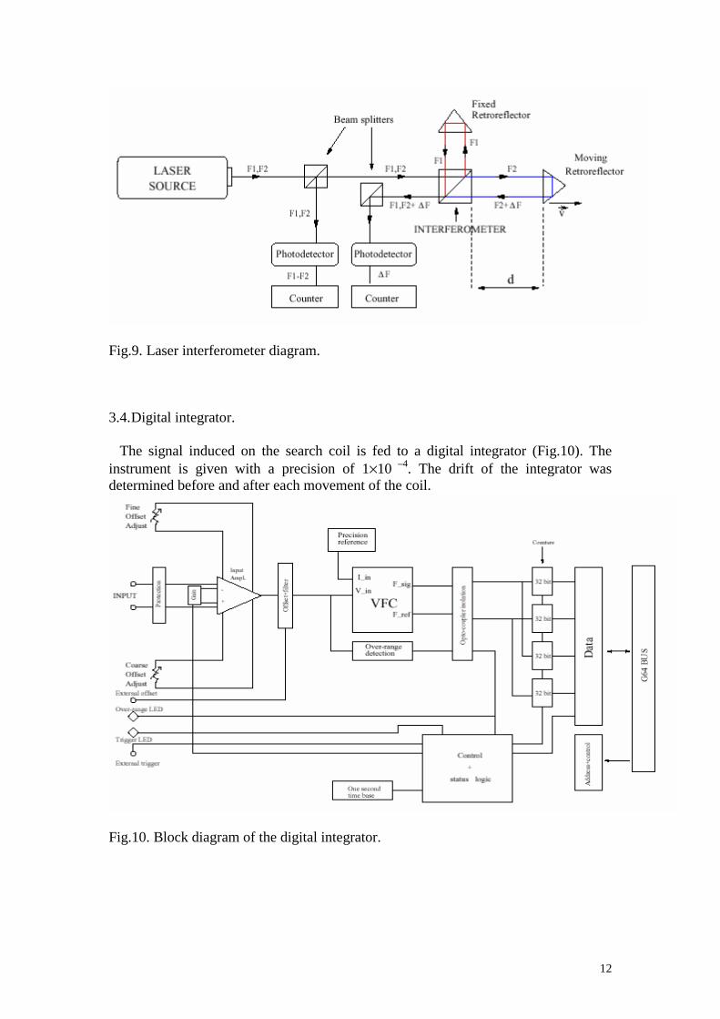
Fig.9. Laser interferometer diagram. 3.4. Digital integrator. The signal induced on the search coil is fed to a digital integrator (Fig.10). The instrument is given with a precision of 1×10 –4. The drift of the integrator was determined before and after each movement of the coil.

Fig.10. Block diagram of the digital integrator.

12

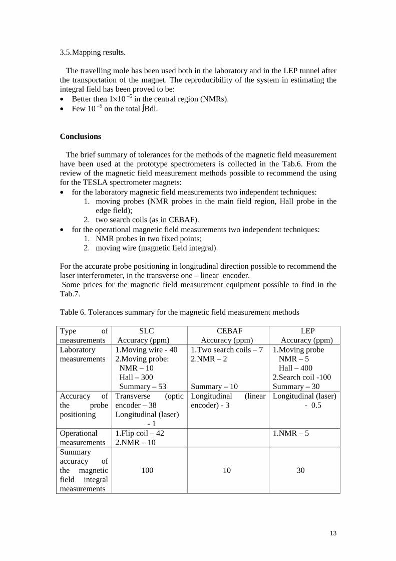
3.5. Mapping results. The travelling mole has been used both in the laboratory and in the LEP tunnel after the transportation of the magnet. The reproducibility of the system in estimating the integral field has been proved to be: • Better then 1×10 –5 in the central region (NMRs). • Few 10 –5 on the total �Bdl. Conclusions The brief summary of tolerances for the methods of the magnetic field measurement have been used at the prototype spectrometers is collected in the Tab.6. From the review of the magnetic field measurement methods possible to recommend the using for the TESLA spectrometer magnets: • for the laboratory magnetic field measurements two independent techniques:

1. moving probes (NMR probes in the main field region, Hall probe in the edge field);

2. two search coils (as in CEBAF). • for the operational magnetic field measurements two independent techniques:

1. NMR probes in two fixed points; 2. moving wire (magnetic field integral).

For the accurate probe positioning in longitudinal direction possible to recommend the laser interferometer, in the transverse one – linear encoder. Some prices for the magnetic field measurement equipment possible to find in the Tab.7. Table 6. Tolerances summary for the magnetic field measurement methods Type of measurements

SLC Accuracy (ppm)

CEBAF Accuracy (ppm)

LEP Accuracy (ppm)

Laboratory measurements

1.Moving wire - 40 2.Moving probe: NMR – 10 Hall – 300 Summary – 53

1.Two search coils – 7 2.NMR – 2 Summary – 10

1.Moving probe NMR – 5 Hall – 400 2.Search coil -100 Summary – 30

Accuracy of the probe positioning

Transverse (optic encoder – 38 Longitudinal (laser) - 1

Longitudinal (linear encoder) - 3

Longitudinal (laser) - 0.5

Operational measurements

1.Flip coil – 42 2.NMR – 10

1.NMR – 5

Summary accuracy of the magnetic field integral measurements

100

10

30

13

Table 7. Prices for the magnetic field measurement equipment Producer Equipment Price METROLAB NMR Teslameter (PT-2025)

Accuracy – 5 ppm (SFr) 21600

Probe multiplexer 6190 Probe multiplexer amplifier 7440 Mini flrxible probe – 4 17760 Mini flrxible probe – 2 6780 Sum 60000 = 42500 € Integrator (PDI-5025) Digital integrator (SFr) 16270 Integrator module 8600 Sum 25000 = 16200 € GMV Flip coil ($) 13500 = 12000 € Group3 Digital Hall effect teslameter Teslameter DTM-151

Accuracy – 100 ppm ($) 3500

High sensitivity Hall probe 1850 Sum 5350 = 4900 €

14