Review of Probability Wilks, Chapter 2 Ji-Sun Kang and Eugenia Kalnay

AOSC630 Spring, 2008, updated in 2017

Definition

§  Event: set, class, or group of possible uncertain outcomes q  A compound event can be decomposed into two or more

(sub) events q  An elementary event cannot be decomposed

§  Sample space (event space), S q  The set of all possible elementary events

§  MECE (Mutually Exclusive & Collectively Exhaustive) q  Mutually Exclusive: no more than one of the events can

occur q  Collectively Exhaustive: at least one of the events will

occur ! A set of MECE events completely fills a sample space

Probability Axioms

§  P(A) ≥ 0 §  P(S) = 1 §  If (E1 E2)=0, i.e., if E1 and E2 exclusive, then P(E1 E2)=P(E1)+P(E2)

∪∩

E1 E2

21 EE ∪

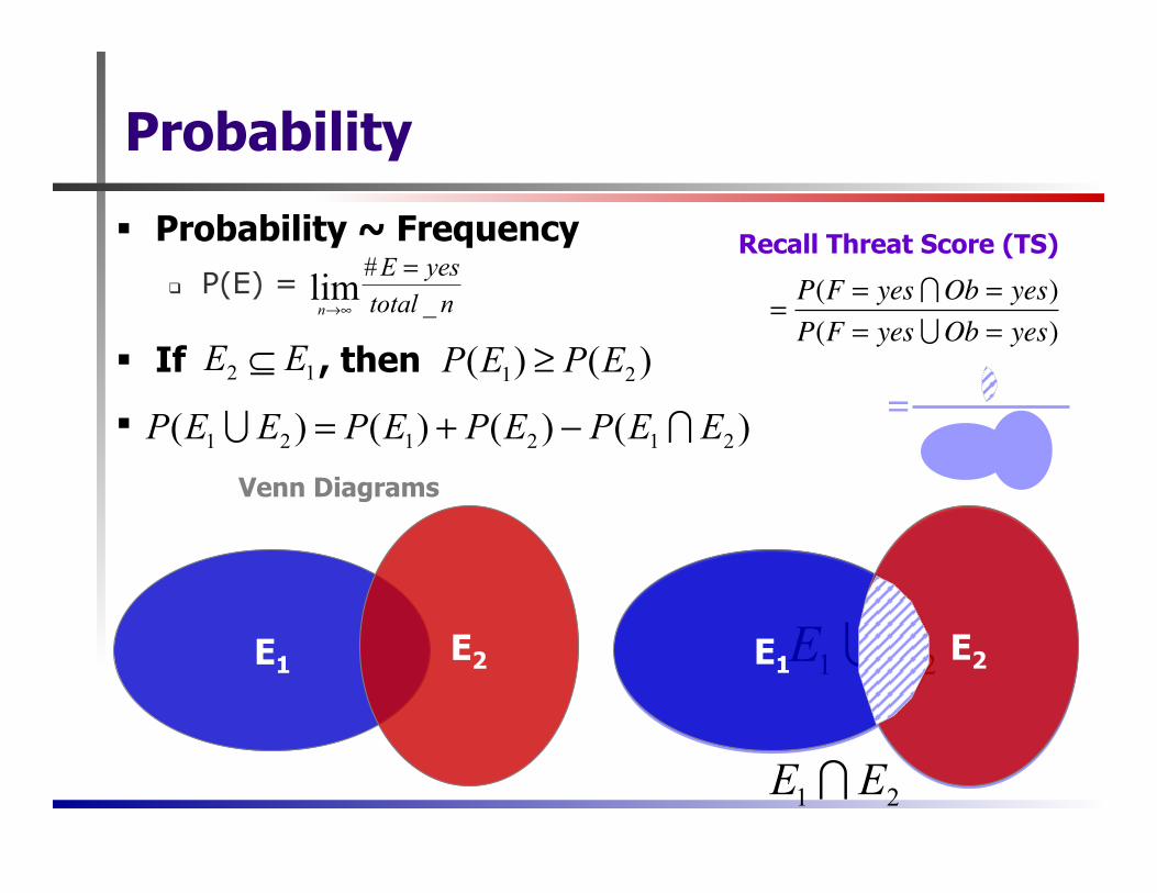
Probability

§  Probability ~ Frequency q  P(E) =

§  If , then

§ 

E1 E2

ntotalyesE

n _#lim =

∞→

12 EE ⊆ )()( 21 EPEP ≥

Venn Diagrams

)()()()( 212121 EEPEPEPEEP ∩∪ −+=

E1 E2

21 EE ∩

Recall Threat Score (TS)

=P(F = yes ∩Ob = yes)P(F = yes ∪Ob = yes)

=

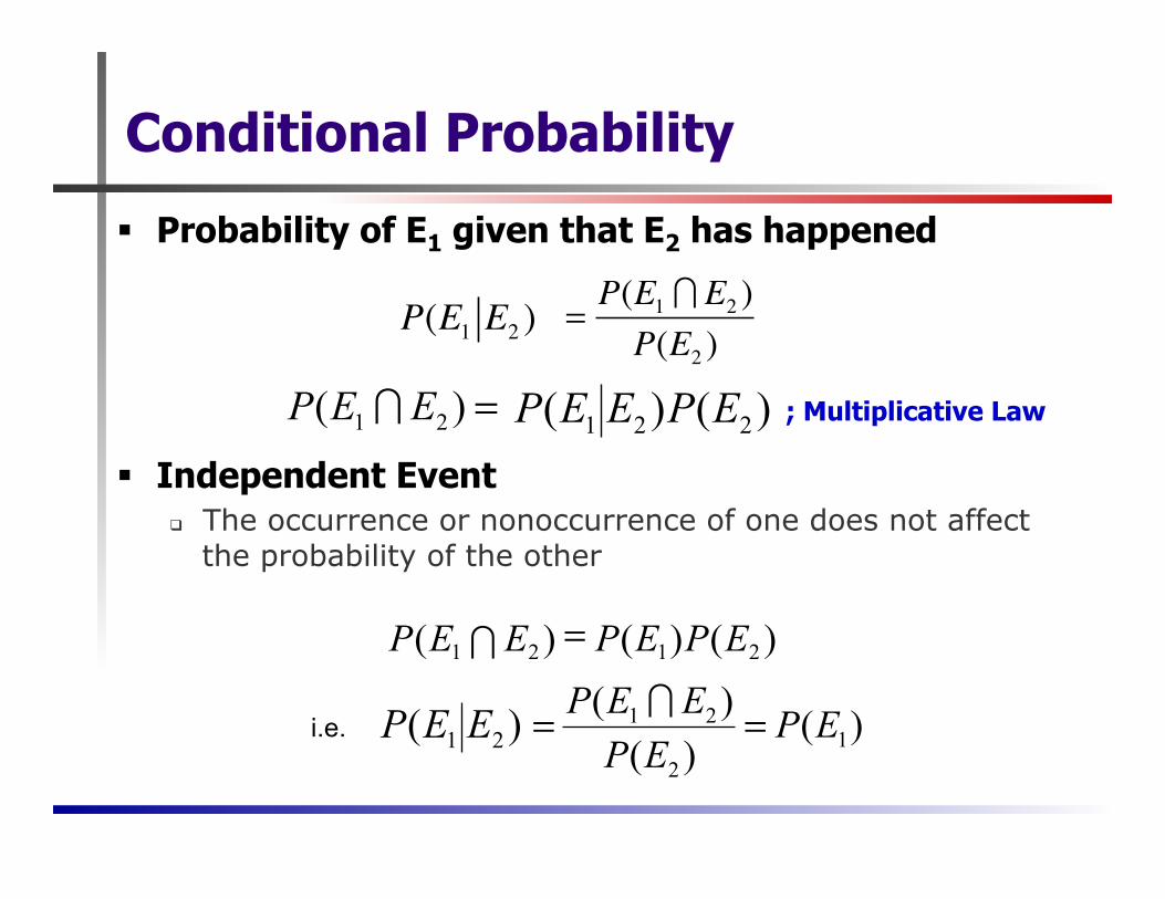
Conditional Probability

§  Probability of E1 given that E2 has happened

§  Independent Event q  The occurrence or nonoccurrence of one does not affect

the probability of the other

P(E1 E2 ) =P(E1 ∩ E2 )P(E2 )

)( 21 EEP )()()(

12

21 EPEPEEP == ∩

i.e.

)()( 221 EPEEP=)( 21 EEP ∩ ; Multiplicative Law

) ( ) ( ) ( 2 1 2 1 E P E P E E P = ∩

Exercise

§  From the Penn State station data for Jan. 1980, compute the probability of precipitation, of T>32F, conditional probability of precipitation if T>32F, and conditional probability of precipitation tomorrow if it is raining today

§  Prove graphically the DeMorgan Laws:

!! P (A∪B)c}{ = P Ac ∩Bc} ;{ P (A∩B)c}{ = P Ac ∪Bc}{

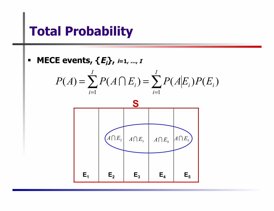
Total Probability

§  MECE events, {Ei}, i=1, …, I

S

E1 E2 E3 E4 E5

2EA∩3EA∩ 4EA∩ 5EA∩

)()()()(1 1

ii

I

i

I

ii EPEAPEAPAP ∑ ∑

= === ∩

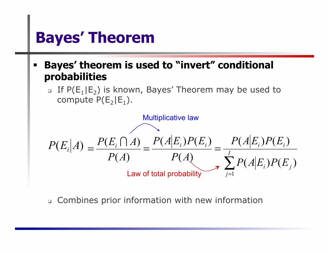
Bayes’ Theorem

§  Bayes’ theorem is used to “invert” conditional probabilities q  If P(E1|E2) is known, Bayes’ Theorem may be used to

compute P(E2|E1).

q  Combines prior information with new information

)( AEP i

∑=

=== I

jji

iiiii

EPEAP

EPEAPAPEPEAP

APAEP

1)()(

)()()(

)()()()( ∩

Multiplicative law

Law of total probability

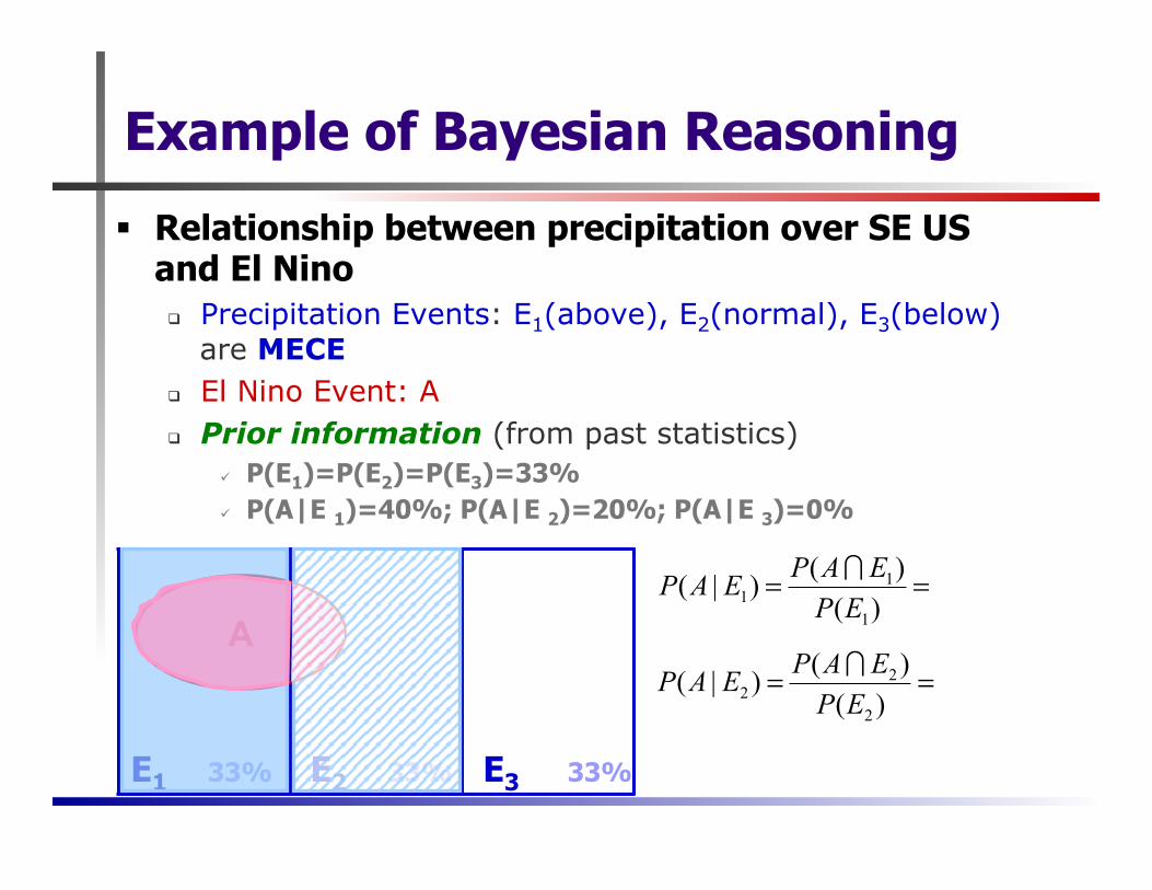
Example of Bayesian Reasoning

§  Relationship between precipitation over SE US and El Nino q  Precipitation Events: E1(above), E2(normal), E3(below)

are MECE q  El Nino Event: A q  Prior information (from past statistics)

ü  P(E1)=P(E2)=P(E3)=33% ü  P(A|E 1)=40%; P(A|E 2)=20%; P(A|E 3)=0%

E1 E2 E3 33% 33% 33%

A ==

)()()|(

1

11 EP

EAPEAP ∩

==)()()|(

2

22 EP

EAPEAP ∩

=0.40

=0.20

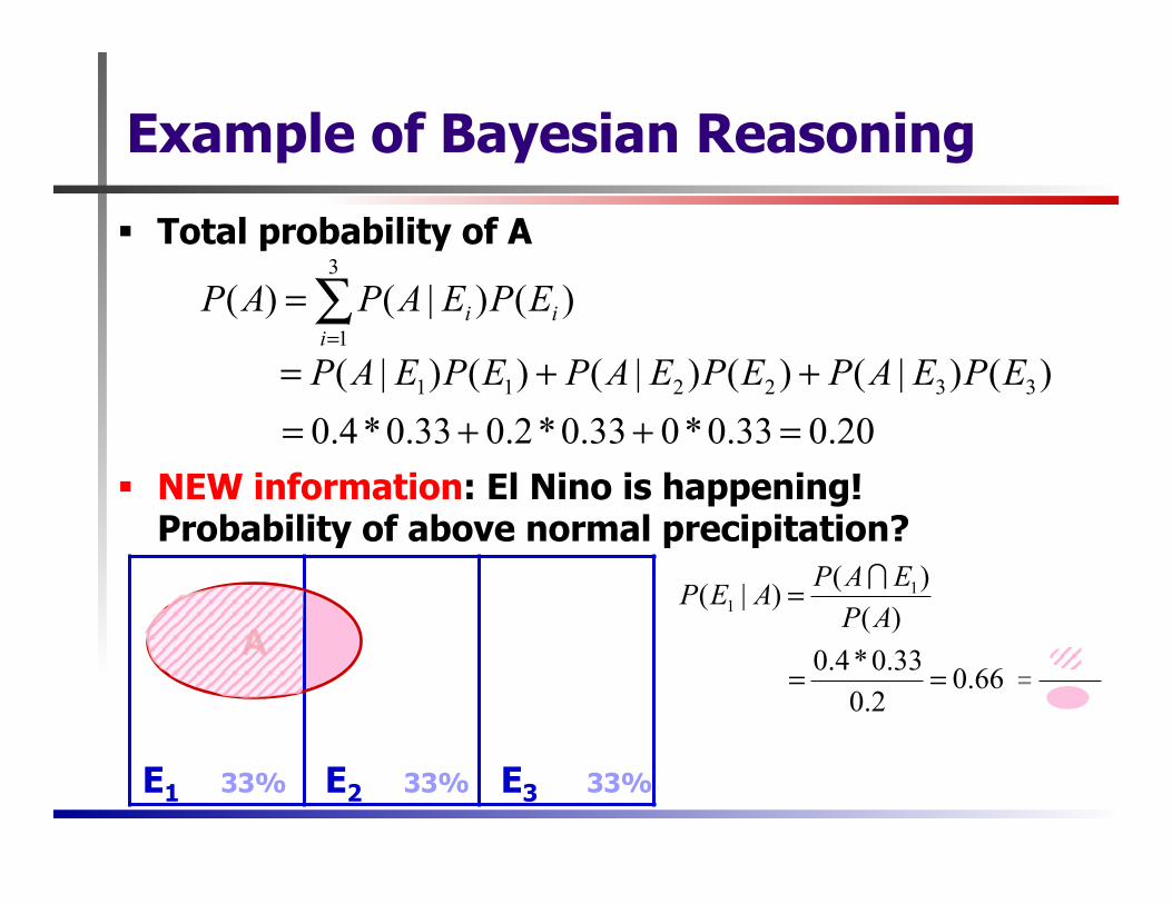
Example of Bayesian Reasoning

§  Total probability of A

§  NEW information: El Nino is happening! Probability of above normal precipitation?

∑=

=3

1)()|()(

iii EPEAPAP

)()|()()|()()|( 332211 EPEAPEPEAPEPEAP ++=20.033.0*033.0*2.033.0*4.0 =++=

E1 E2 E3 33% 33% 33%

A )()()|( 1

1 APEAPAEP ∩=

66.02.033.0*4.0 == =

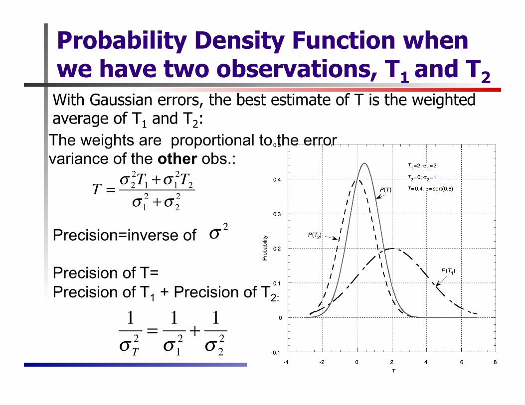
Probability Density Function when we have two observations, T1 and T2

T = σ 22T1 +σ 1

2T2σ 12 +σ 2

2

1σ T2 =

1σ 12 +

1σ 22

Precision=inverse of Precision of T= Precision of T1 + Precision of T2:

The weights are proportional to the error variance of the other obs.:

With Gaussian errors, the best estimate of T is the weighted average of T1 and T2:

σ 2

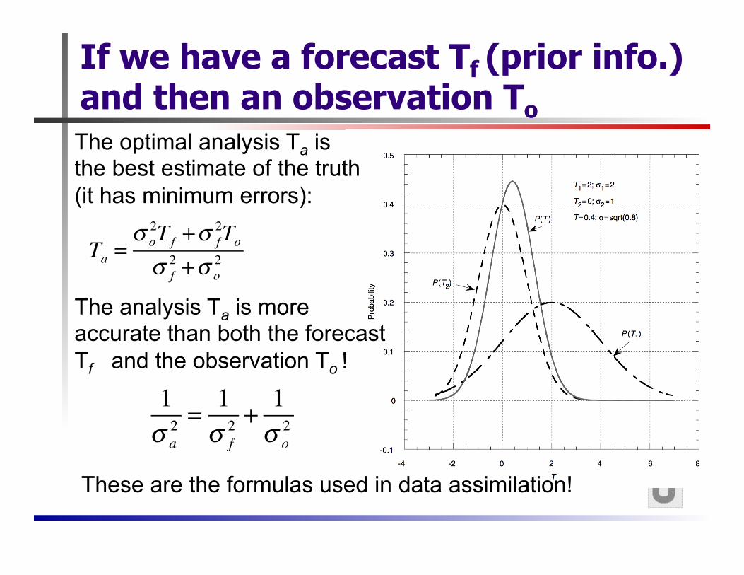
If we have a forecast Tf (prior info.) and then an observation To

Ta =σ o2Tf +σ f

2Toσ f2 +σ o

2

1σ a2 =

1σ f2 +

1σ o2

The analysis Ta is more accurate than both the forecast Tf and the observation To !

The optimal analysis Ta is the best estimate of the truth (it has minimum errors):

These are the formulas used in data assimilation!

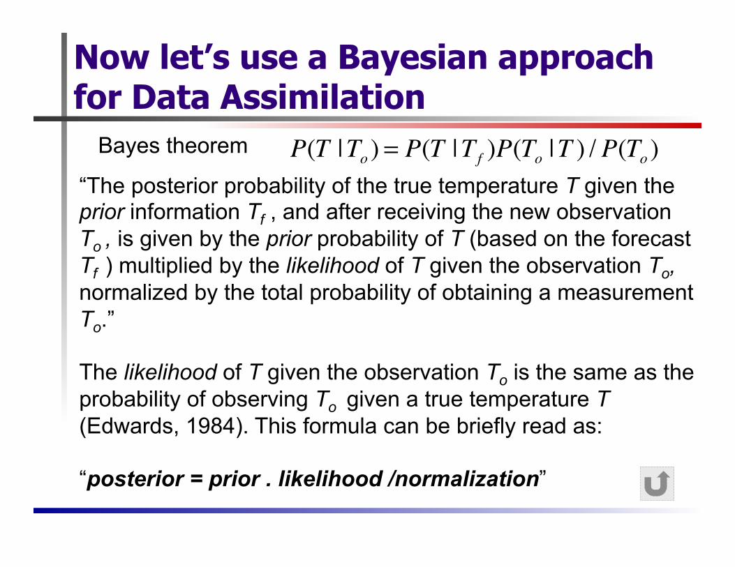
Now let’s use a Bayesian approach for Data Assimilation

P(T |To ) = P(T |Tf )P(To |T ) / P(To )Bayes theorem

“The posterior probability of the true temperature T given the prior information Tf , and after receiving the new observation To , is given by the prior probability of T (based on the forecast Tf ) multiplied by the likelihood of T given the observation To, normalized by the total probability of obtaining a measurement To.” The likelihood of T given the observation To is the same as the probability of observing To given a true temperature T (Edwards, 1984). This formula can be briefly read as: “posterior = prior . likelihood /normalization”

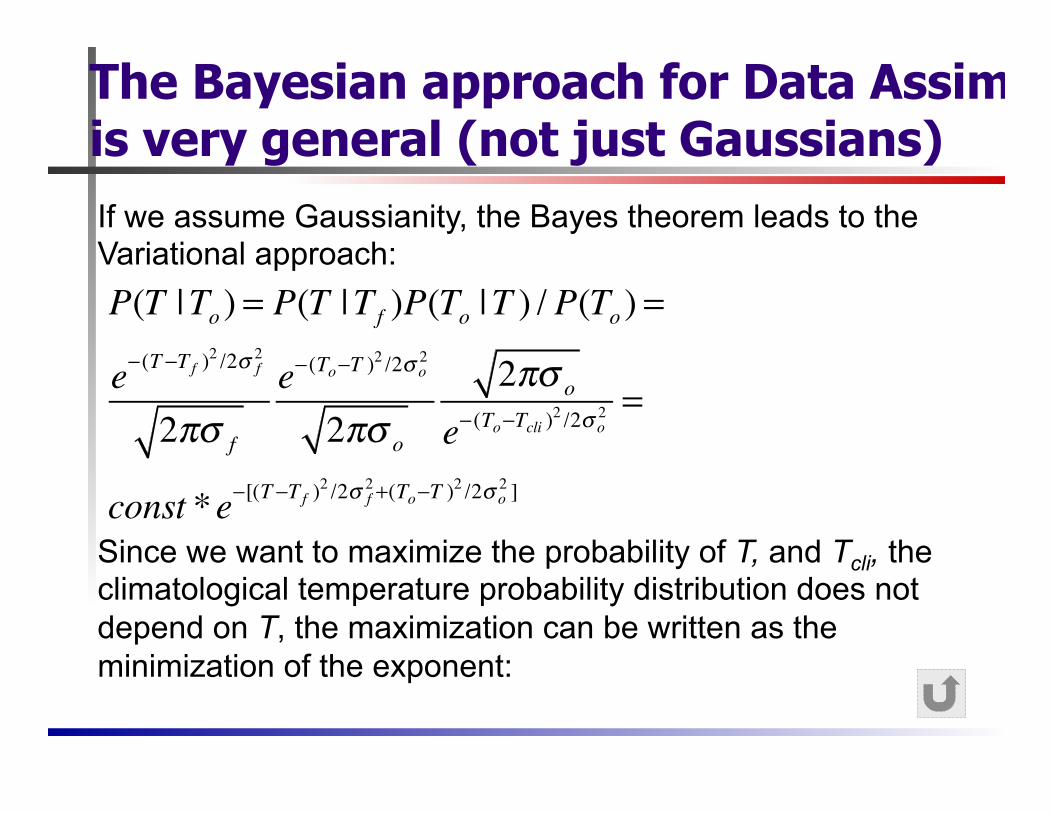
The Bayesian approach for Data Assim is very general (not just Gaussians)

If we assume Gaussianity, the Bayes theorem leads to the Variational approach: P(T |To ) = P(T |Tf )P(To |T ) / P(To ) =

e−(T −Tf )2 /2σ f

2

2πσ f

e−(To−T )2 /2σ o

2

2πσ o

2πσ o

e−(To−Tcli )2 /2σ o

2 =

const *e−[(T −Tf )2 /2σ f

2+(To−T )2 /2σ o

2 ]

Since we want to maximize the probability of T, and Tcli, the climatological temperature probability distribution does not depend on T, the maximization can be written as the minimization of the exponent:

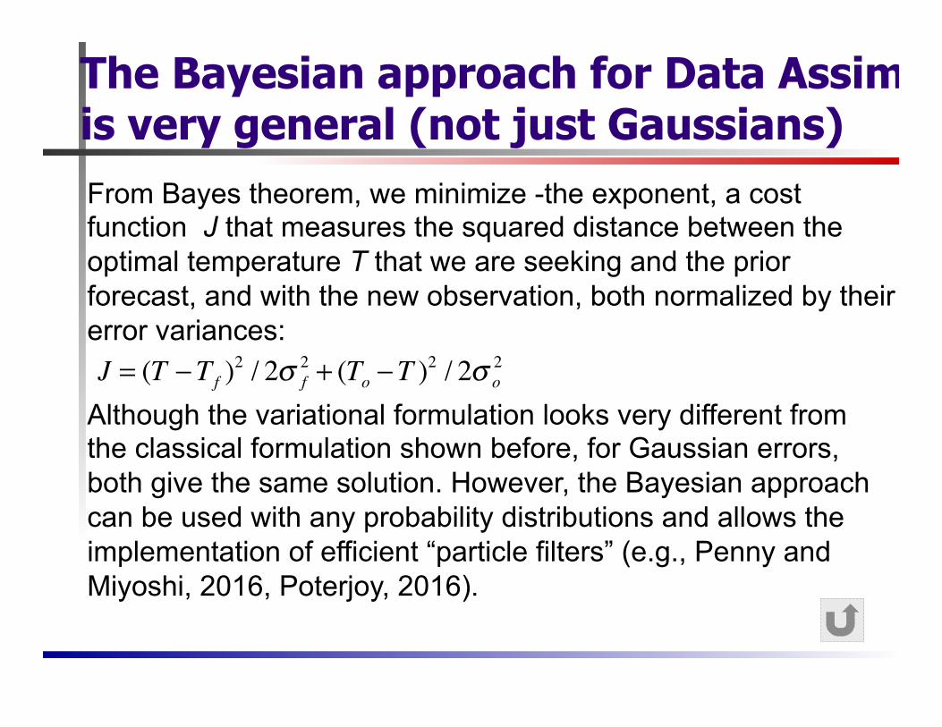
The Bayesian approach for Data Assim is very general (not just Gaussians)

From Bayes theorem, we minimize -the exponent, a cost function J that measures the squared distance between the optimal temperature T that we are seeking and the prior forecast, and with the new observation, both normalized by their error variances:

Although the variational formulation looks very different from the classical formulation shown before, for Gaussian errors, both give the same solution. However, the Bayesian approach can be used with any probability distributions and allows the implementation of efficient “particle filters” (e.g., Penny and Miyoshi, 2016, Poterjoy, 2016).

J = (T −Tf )2 / 2σ f

2 + (To −T )2 / 2σ o

2