Embed Size (px)
Citation preview
Review of Dispersion Modellingfor Odour Predictions
Science Report: SC030170/SR3
SCHO0307BMKQ-E-P

Review of Dispersion Modelling for Odour Predictionsii
The Environment Agency is the leading public body protecting andimproving the environment in England and Wales.
It’s our job to make sure that air, land and water are looked after byeveryone in today’s society, so that tomorrow’s generations inherit acleaner, healthier world.
Our work includes tackling flooding and pollution incidents, reducingindustry’s impacts on the environment, cleaning up rivers, coastalwaters and contaminated land, and improving wildlife habitats.
Published by:Environment Agency, Rio House, Waterside Drive, Aztec West,Almondsbury, Bristol, BS32 4UDTel: 01454 624400 Fax: 01454 624409www.environment-agency.gov.uk
ISBN: 978-1-84432-718-8
© Environment Agency March 2007
All rights reserved. This document may be reproduced with priorpermission of the Environment Agency.
The views expressed in this document are not necessarily thoseof the Environment Agency.
This report is printed on Cyclus Print, a 100% recycled stock,which is 100% post consumer waste and is totally chlorine free.Water used is treated and in most cases returned to source inbetter condition than removed.
Further copies of this report are available from:The Environment Agency’s National Customer Contact Centreby emailing [email protected] or bytelephoning 08708 506506.
Authors:Dr Jon Pullen, Dr Yasmin Vawda
Dissemination Status: Publicly available
Keywords:Odour Modelling, Odour Dispersion, Odour Cluster
Research Contractor:Dr Yasmin Vawda Tel: 0207 902 6166Bureau VeritasGreat Guildford House30 Great Guildford StreetLondonSE1 0ES
Environment Agency’s Project Manager:Neil Heptinstall, AQMAU, Cambria House
Science Project Number: SC030170
Product Code: SCHO0307BMKQ-E-P

Review of Dispersion Modelling for Odour Predictions iii
Science at the Environment Agency
Science underpins the work of the Environment Agency, by providing an up to dateunderstanding of the world about us, and helping us to develop monitoring toolsand techniques to manage our environment as efficiently as possible.
The work of the Science Group is a key ingredient in the partnership betweenresearch, policy and operations that enables the Agency to protect and restore ourenvironment.
The Environment Agency’s Science Group focuses on five main areas of activity:
• Setting the agenda: To identify the strategic science needs of the Agency toinform its advisory and regulatory roles.
• Sponsoring science: To fund people and projects in response to the needsidentified by the agenda setting.
• Managing science: To ensure that each project we fund is fit for purpose andthat it is executed according to international scientific standards.
• Carrying out science: To undertake the research itself, by those best placed todo it - either by in-house Agency scientists, or by contracting it out touniversities, research institutes or consultancies.
• Providing advice: To ensure that the knowledge, tools and techniquesgenerated by the science programme are taken up by relevant decision-makers,policy makers and operational staff.
Steve Killeen Head of Science
Review of Dispersion Modelling for Odour Predictioniv
Executive SummaryThe Environment Agency’s draft report Horizontal Guidance for Odour, H4(Environment Agency 2002a) sets out an approach for quantifying odourannoyance, using a series of phases. These are estimation of odour releasevalue, dispersion modelling to estimate the odour exposure, correlation of thepredicted exposure against the expected degree of annoyance (using IndicativeOdour Exposure Standards, IOES) and correlation with negative copingbehaviours (nuisance and complaint). There are uncertainties associated witheach step of this assessment process. This study has examined the componentuncertainties by means of a detailed literature review, and identified theirrelative significance. An attempt is made at ranking the component uncertaintieswhere possible using hypothetical, simplified scenarios.
This desk-top study has shown that not all of the information is available forquantifying the component uncertainties. However, this review provides a“model” of how the component uncertainties for each phase are inter-related.This could enable the Environment Agency to slot-in missing information as itbecomes available from future research (or use professionaljudgement/consensus in the mean-time). In this sense, this report does providea step forward in the practical understanding of the importance of the differentphases of work that comprise an H4 assessment.
Source strength
The dispersion model requires the odour source strength as a key input. Themost reliable value for this input could, in theory, be determined from a largenumber of periodic dynamic dilution olfactometric (DDO) measurements, on asingle existing chimney, where the release is controlled, continuous, and doesnot vary with time or process cycle. The uncertainty escalates sharply forestimated odour emission rates, time-varying emissions, multiple sources on asite, and when specific compounds are used as surrogates for the total odour.
DDO is not currently practical on a continuous basis for any source. Theinability to accurately quantify the odour’s temporal variation, and difficulties incorrelating the source variation with time-varying meteorology in the dispersionmodelling, is the most significant source of uncertainty in the majority of odourassessments.
There are many components in the derivation of the source strength value forwhich a numerical estimate of uncertainty cannot be quoted. These are verysituation-specific. The uncertainty on the source strength value can be severalorders of magnitude even for commonly-encountered situations with time-varying emissions and/or estimates based on surrogate compounds or emissionfactors.
Review of Dispersion Modelling for Odour Predictions v
Dispersion Modelling of Exposure
It is important to recognise that the uncertainties associated with modellingsome types of odorous release (e.g. diffuse/fugitive area sources, non-verticalvents) are very large. In such cases, the use of dispersion modelling as anassessment tool should be questioned.
The results of different, new-generation models can vary by up to a factor of 8,for high percentile calculations with significant building wake effects.Examination of the range of results provides a sensitivity analysis of the modelalgorithms, and provides greater confidence in any regulatory decision.Dispersion modelling is usually carried out when the risk of odour annoyance ishigh. Under these circumstances, the use of more than one dispersion modelcan be justified for a risk-based approach.
There is an urgent need to verify, for UK situations, the Dutch dose-responserelationship which was established historically for livestock units. This isbecause almost no details are available on the dispersion model which wasused to establish this empirical dose-response curve, nor the input data for thatmodelling. Of particular concern is the reliability of the source strength data thatwere used for the Dutch modelling.
There are many components of the dispersion modelling process for which anumerical estimate of ‘typical’ uncertainty cannot be quoted. These aresituation-specific, e.g. when complex terrain is present.
Dispersion models are currently in practical use only for predicting ‘ensemblemean’ (typically hourly mean) concentrations. Fluctuation modelling is not yetadequately validated. As long as this remains the case, the ‘Type 2’ approachfor odour assessment set out in Draft H4 (hourly mean modelling comparedagainst an empirical benchmark) must remain the only feasible option.
ADMLC has provided detailed guidance on best practice for dispersionmodelling. Most of the guidelines are applicable to odour modelling. It would beuseful if more detailed guidance was incorporated into Draft H4, giving a clearersteer towards the required level of transparency and rigour in odourassessments. Also, some uniformity in the way that model sensitivity anduncertainty are expressed would be useful.
Correlation with annoyance
The uncertainty in the correlation of odour exposure with odour annoyance is acombination of two types of component uncertainties: random (which areprecision-type uncertainties, responsible for the scatter and the correlationcoefficient found for the dose-response curve), and systematic (which are thebias or accuracy-type uncertainties that include factors such as how relevantthe Dutch pig-odour response curve is to other odour types in UK conditions,and how appropriate the concentration levels for the ‘offensiveness’ bands havebeen set).

Review of Dispersion Modelling for Odour Predictionvi
If a series of dose-response studies had been carried out under UK conditions,it would have allowed the repeatability of the Draft H4 method to be estimated.Unfortunately no such studies have been carried out.
The use of a calibration curve derived from Dutch livestock odours, andapplying it to other odours and other types of installation in different countries,presents an additional layer of uncertainty compared to deriving a modellingguideline from a bespoke, dose-response study. However, again it is notpossible to place any numerical estimates of the magnitude of this additionallayer of uncertainty, as it is situation-specific. For a livestock installation theadditional layer of uncertainty might be expected to be small. For other, verydifferent, odours or installations, the leap of faith is wider and the additionaluncertainty may be much larger. Practitioners must make themselves aware ofthis, and form a qualitative view on the significance of this component ofuncertainty.
On the positive side, the level of annoyance measured by a survey in NewZealand (Ministry for the Environment 2002) was found to be consistent with theodour dose—community-response curves reported for the Netherlands(Miedema 1992). The dose-response curves, although developed for otherindustries and using a Dutch community response, appeared to be valid for pulpmill odours in New Zealand.
The Draft H4 guidance states that the above benchmarks are indicativestandards and that UK dose-effect studies are planned. It also states elsewherein the document that “the only realistic way of estimating the actual level ofannoyance in a particular community resulting from exposure is by carrying outdose-response studies locally”. However, Draft H4 appears much less explicitthan the New Zealand guidance in highlighting the “interim” nature of thesegeneric-type odour guidelines and that they should ideally be superseded byindustry-specific guidelines developed from bespoke dose-response studies.
It is possible that some dose-response studies will be performed around wastemanagement facilities as part of a study into defining loss of amenity throughodour, carried out as part of Defra`s Waste Research R&D programme*. Thereis also a possibility of UK Water Industry Research (UKWIR) coordinating somestudies around wastewater treatment plants to support the water industry inmeeting the Defra Code of Practice on Odour Nuisance from SewageTreatment Works.
Correlation with nuisance and complaintsThe Environmental Protection Act (EPA) 1990 contains no technical definitionsof nuisance, such as maximum concentrations, frequencies or durations ofodour in air. This needs to be addressed, together with a nuisancemeasurement methodology, before any estimate of the uncertainty in thecorrelation with odour exposure can be made.
* Details at http://www.defra.gov.uk/environment/waste/wip/research/index.htm

Review of Dispersion Modelling for Odour Predictions vii
Complaints are more usually measured directly by complaints monitoring, ratherthan being predicted. However, dose-response studies using complaints as theresponse measurand have been carried out in New Zealand and Australia, butusing different models to those in common use in the UK, and using differentpercentiles to describe exposure.The uncertainties in correlating predicted exposure with either nuisance orcomplaints levels would be considerably higher than for annoyance, due to theadditional factors involved.
Review of Dispersion Modelling for Odour Predictionviii
ContentsExecutive Summary iv
Contents viii
1 Introduction 11.1 Scope and status of this report 11.2 Background and overall aim of the project 11.3 Objectives of the Study 11.4 Applications and limitations 21.4.1 Using the information on uncertainty 21.4.2 Source-types covered by this study 3
2 Methodology 52.1 Overall approach to the investigation 52.2 Literature review 5
3 The Component Steps in the Annoyance Process 6
4 Phase I – Estimation of Odour Release Value 114.1 Overview of the odour release process 114.2 Summary of the component uncertainties in the odour release rate value 124.3 Uncertainties associated with the application of the technique 154.3.1 Temporal uncertainties 154.3.2 Spatial uncertainties 194.4 Uncertainties associated with the technique itself 204.4.1 Component uncertainties when measurements of odour emissions are
used 204.4.2 Component uncertainties when estimates of odour emissions are used 344.5 Summary of the uncertainties in the odour release rate value 40
5 Phase II – Modelling Odour Exposure 435.1 Atmospheric dispersion modelling 435.2 Ways of reporting modelling uncertainties 475.3 Is detailed modelling appropriate? 495.4 ‘Old-Generation’ models: COMPLEX1 and LTDF 505.5 ‘New-Generation’ models: ADMS and AERMOD 515.6 Model inter-comparison studies 535.7 Model inter-comparison results with building downwash effects 645.8 Choice of model 655.9 Treating predictions from more than one model 665.10 Defining model input parameters 66
Review of Dispersion Modelling for Odour Predictions ix
5.10.1 Source location 665.10.2 Horizontal releases 675.10.3 Capped release points 675.10.4 Multiple sources 685.10.5 Area and near-ground sources 695.11 Peak-to-mean ratios 715.12 Fluctuations Models 725.13 High percentiles 755.14 Meteorology 765.15 Terrain height 795.16 Location of receptors 805.17 Summary of the uncertainties in the modelled exposure 80
6 Phase III: Correlation with Annoyance 836.1 Overview of this phase 836.2 Bespoke odour exposure guideline standards derived from industry-specific
dose-response studies 846.2.1 Summary of the component uncertainties in industry-specific guidelines 846.2.2 Uncertainties associated with the application of the dose-response study 856.2.3 Uncertainties associated with the dose-response study technique itself 896.3 Using default Indicative Odour Exposure Standards 906.3.1 Background to the Summary Indicative Odour Exposure Standards 906.3.2 Comments on the additional uncertainties with Indicative Odour Exposure
Standards 926.4 Summary of uncertainty in correlation with annoyance 95
7 Phase IV: – Correlation with Negative Coping Behaviours (Nuisanceand Complaints 98
7.1 Adverse outcomes of odour exposure – annoyance, nuisance, complaints98
7.2 Correlation of exposure with nuisance and complaints 1007.3 Complaints analysis 1017.4 Summary of uncertainty in correlation with nuisance and complaints 101
8 Main Findings 1038.1 Source strength 1038.2 Dispersion Modelling of Exposure 1048.3 Correlation with annoyance 1048.4 Correlation with nuisance and complaints 106
9 Recommendations 1099.1 Determination of Source Strength 1099.2 Odour emission factors 1099.3 Dispersion modelling 109

Review of Dispersion Modelling for Odour Predictionx
9.4 Model inter-comparison 1109.5 Dutch livestock modelling 1109.6 Fluctuations 1109.7 UK epidemiological dose-effect survey 1119.8 Is detailed modelling appropriate? 1119.9 Information required by Draft H4 1129.10 A Checklist for Inspectors 112
Abbreviations and acronyms 113
Appendix A – Assessment of Uncertainty of Stack Emissions 116i and ii Specification and identification of the sources of uncertainty 116iii Quantifying the uncertainties 119A.3 The Uncertainty Budget Approach 121
References 124

Review of Dispersion Modelling for Odour Predictions 1
1 Introduction
1.1 Scope and status of this report
This Project, Review of dispersion modelling for odour predictions, is one of acluster of three projects funded by the Environment Agency’s ScienceDepartment (reference 13933), managed by Bureau Veritas (BV). BV providedthe Environment Agency with a proposal and Work Plan for Project 3 on 1st
November 2005, in accordance with the Technical Specification dated 12thOctober 2005 from Dr Damien Rosser. The proposal committed BV to providingthe Environment Agency with a report summarising the findings of aninvestigation into the uncertainties associated with using atmospheric dispersionmodelling to assess odour exposure, and extrapolation to annoyance.
1.2 Background and overall aim of the project
In October 2002, the Environment Agency published its draft Technical GuidanceNote H4 (Draft H4) (Environment Agency 2002a). This guidance described anapproach to assessing and regulating odour impacts, involving quantifying odouremissions, dispersion modelling to estimate odour exposure, and correlation ofexposure with the expected degree of annoyance using “Indicative OdourExposure Standards” (numerical air quality criteria for odour). The approach canbe used directly to assess the annoyance impact of an installation. Alternatively,it can be worked backwards from an “acceptable” level of annoyance to derivethe maximum emission limit value (ELV) for odour at source that can be set as aPollution Prevention and Control (PPC) Permit condition that will avoid“reasonable cause for annoyance”.
The approach contains a number of more or less discrete steps, each having itsown component uncertainty. It is important to be able to understand howimportant these component uncertainties are, which ones dominate, and whichones are relatively insignificant. This project aims to provide a betterunderstanding of the likely relative importance of the various steps in the Draft H4approach, in terms of their uncertainties. Ultimately, the findings of this projectcould assist in improving the Draft H4 method, by ensuring that effort in revisionsis targeted at those uncertainties which are most important for permittingdecisions.
1.3 Objectives of the StudyThis review focuses on installations for which predictive dispersion modelling maybe used, as part of a detailed odour impact assessment for PPC permitting. Thesemay be existing installations with an existing or potential odour problem; or theymay be proposed installations with potential odour problems. The drivers for thisreview of uncertainties are as follows:
Review of Dispersion Modelling for Odour Prediction2
a) Appendix 3 of Draft H4 Part 1 states that a sensitivity analysis of modelpredictions for critical model input parameters should be carried out.Conclusions and assessment need to take into account uncertainties in modelpredictions. Both the operator and regulator need to have confidence in theoutcome of the dispersion modelling.
b) If modelling shows that the Draft H4 Indicative Odour Exposure Standards(IOES) are, or are not, met, there needs to be confidence in the certainty ofthis prediction. The uncertainties in the source strength and the modellingneed to be identified.
c) Also, there has to be confidence that the Indicative Odour ExposureStandards really do represent ‘no reasonable cause for annoyance’ for thegiven situation. This requires a review of how the Indicative Odour ExposureStandards were derived, and how applicable they are to the situation beingmodelled. A review of the derivation the Indicative Odour Exposure Standardshas been carried out in the Literature Review for Project 2 of this ScienceProject (Environment Agency 2007b).
1.4 Applications and limitations
1.4.1 Using the information on uncertainty
This study seeks to examine the uncertainty (U) in the main stages of an odourimpact assessment that follows the Draft H4 approach. Particular attention isgiven to:
• the value for source strength used in the dispersion model (discussed atlength in Chapter 4);
• the differences between the predictions of different models. These areimportant, because the Draft H4 Indicative Odour Exposure Standardswere set on the basis of results from a particular type of dispersionmodelling exercise (based on an ‘old-generation’ model) in theNetherlands (discussed at length in Chapter 5). Different (i.e. ‘new-generation’) models are now used in the UK and elsewhere for odourassessment.
The relative magnitudes of the component uncertainties (in the source strength,in the modelling results, and in the assessment criterion) need to be examined inorder to prioritise future research and audit effort.
A realistic outcome of this review is not so much to get a precise estimate of theoverall uncertainty, but rather to investigate the relative importance of the maincomponent uncertainties. It should be possible to identify, for example, if thedispersion modelling has a much more significant component uncertainty thanemissions quantification, or assignment to different bands of unpleasantness.
Review of Dispersion Modelling for Odour Predictions 3
1.4.2 Source-types covered by this study
There are three main categories of industrial releases to atmosphere.
• Controlled releases – the emissions are managed in some way, either aspart of a process or as part of a control/ abatement mechanism and theemissions are therefore quantifiable. Most (but not all) controlled releases arefrom point sources: BS EN 17025 defines a point source as a discretestationary source of waste gases to atmosphere through canalised ducts ofdefined dimension and air flow rate (e.g. chimneys, vents).
• Diffuse releases - BS EN 17025 defines diffuse sources as those withdefined dimensions (mostly surface sources) which do not have a definedwaste-air flow, such as waste dumps, lagoons, fields after manure spreading,un-aerated compost heaps.
• Fugitive releases – these are, literally, releases that cannot be captured. BSEN 17025 defines fugitive sources as elusive or difficult to identify sources,releasing undefined quantities of odorants (e.g. valve and flange leakage,passive ventilation apertures). They are uncontrolled and often dependent onexternal conditions (e.g. wind) which make them difficult to quantify with anyreasonable degree of certainty. Another definition of a fugitive emission is arelease that is unintentional. An oil refinery may have a quarter of a millionpumps, valves and flanges that potentially can leak, making it impractical tomeasure the emissions from every source.
Industrial releases to atmosphere can also be subdivided in terms of their spatialcharacteristics, usually as a point source, line source or area source. It isimportant to recognise that these can be controlled releases, diffuse releases orfugitive releases, as shown in the table below. However, it is controlled pointsources (e.g. chimney stacks and vents) that are most commonly monitored andmodelled.

Review of Dispersion Modelling for Odour Prediction4
Table 1.1 Categories of emissions to atmospherePoint source Line source Area source
Controlledrelease
Emissions from fixed-location plant andoften (but not always)released toatmosphere via avent, duct or chimneystack
Tail-pipe emissionsfrom vehicles drivingalong a road
Diffuserelease
Open process tanks Open gullies andculverts
Landfill surfaces,lagoons, compostheaps
Fugitiverelease
Intermittently leakingvalve
Dust re-suspendedin a vehicle’s wake;wind-whipping ofdusty material on anopen conveyor belt
Wind-whipping ofa stockpile ofdusty material
The main focus of the discussion in this study is on controlled point-sourcereleases of odour, because this is the main application of the Draft H4 modellingapproach. The discussion is not designed to be focussed on diffuse or fugitivesources, as the Draft H4 approach, using modelling to back-calculate permissibleELVs, is not applicable to such situations. However, for the sake ofcompleteness, some limited comments on other source types are included, as itis recognised that the Environment Agency will, from time to time, receiveEnvironmental Impact Assessments (EIAs) that include odour impact predictionsfor diffuse (usually area) sources.
Emissions factors and mass balance calculations are applied most commonly todiffuse sources and fugitive sources that are difficult to monitor. For similarreasons, the Draft H4 approach using modelling to back-calculate permissibleELVs, is not applicable to emission factor and mass balance calculations, andonly limited comments have been made on these.
Review of Dispersion Modelling for Odour Predictions 5
2 Methodology
2.1 Overall approach to the investigation
It was agreed with the Environment Agency that this investigation would be adesk-top study, based upon a detailed literature review. No practicalinvestigations have been carried out using, for example, sampling, analysis ordispersion modelling.
2.2 Literature review
The objectives of Project 3 were designed to be met by a literature review of theavailable and most up-to-date UK and international scientific literature pertainingto the steps comprising an odour impact assessment which includes dispersionmodelling, with a view to assessing the uncertainties at every step.
Draft H4 was published by the Environment Agency in October 2002, using thebest information and data which were available at the time. It is desirable forProject 3 to focus on relevant new work published after the issue of Draft H4.Relevant publications which are more recent than October 2002 have beenidentified via a ‘Google’ search. Copies of all documents are available to theEnvironment Agency from BV on request.
Several key publications contain information which was the most up-to-date atthe time that they were published. However, certain findings can no longer beconsidered as entirely relevant. Notable as an example are papers whichdescribe model inter-comparison studies; the versions of most models mentionedin the papers have inevitably been superseded (Hall et al 2000a). This isdiscussed in more detail in Chapter 5.
Review of Dispersion Modelling for Odour Prediction6
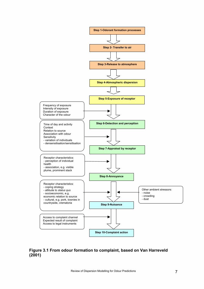
3 The Component Steps in theAnnoyance ProcessIn examining the uncertainty (U) associated with a measurement or estimationprocess, the first task is to break it down into discrete parts to simplify the task.The component uncertainties of these stages can then be investigated and, ifrequired, combined to give an estimate of the overall, total U.Van Harreveld (2001) proposed a conceptual flowchart (which has been set outin previous Environment Agency (2000b) documents) showing the relationshipbetween exposure to malodour and its potential effects on a human population;this is reproduced in Figure 3.1. The contributing factors and the effects, whichmay result ultimately in complaints, are far from straightforward and few of therelationships are completely understood. The main factors, discussed in detail inthe Literature Review for Project 2, were summarised by Van Harreveld as:
• the characteristics of the odour that is released, i.e. detectability (odourconcentration), intensity, hedonic tone, and annoyance potential;
• variable dilution in the atmosphere through turbulent dispersion(turbulence or stability of boundary layer, wind direction, wind speed, etc.);
• exposure of the receptors in the population (this will be dependent on theodour concentration in the ambient air and also the frequency and durationof episodes, influenced by the location of residences, movement ofpeople, time spent outdoors, etc.);
• context of perception (e.g. other odours, background of odours, activityand state of mind within the perception context);
• receptor characteristics (exposure history, association with risks, activityduring exposure episodes, and psychological factors such as toleranceand expectations of the exposed subjects, their coping behaviour, theirperceived threats to their health).
Once exposure to odour has occurred, the process that may lead to annoyance,nuisance and possibly complaints, will involve many psychological and socio-economic factors. These factors, and technical definitions for the termsannoyance and nuisance, are described in the Literature Review for Project 2.
The Literature Review for Project 2 (Environment Agency 2007b) describes thefactors that determine the impact of an odour: whether an odour has anobjectionable effect depends not just on the strength of the odour, but also itsfrequency, intensity, duration, offensiveness (the character and unpleasantness –hedonic tone – at a particular intensity) and location of the receptors. Theseattributes, known collectively as the FIDOL factors, need to be incorporated into(or otherwise accounted for in) the numerical benchmark criterion.
Review of Dispersion Modelling for Odour Predictions 7
Figure 3.1 From odour formation to complaint, based on Van Harreveld(2001)
Step 1-Odorant formation processes
Step 2- Transfer to air
Step 3-Release to atmosphere
Step 4-Atmospheric dispersion
Step 5-Exposure of receptor
Step 6-Detection and perception
Step 7-Appraisal by receptor
Step 8-Annoyance
Step 9-Nuisance
Step 10-Complaint action
Access to complaint channelExpected result of complaintAccess to legal instruments
Receptor characteristics:- coping strategy- attitude to status quo- socioeconomic, e.g.economic relation to source- cultural, e.g. pork, townies incountryside, crematoria
Other ambient stressors:- noise- crowding- dust
Receptor characteristics:- perception of individualhealth- association, e.g. visibleplume, prominent stack
Frequency of exposureIntensity of exposureDuration of exposureCharacter of the odour
Time of day and activityContextRelation to sourceAssociation with odourSensitivity- variation of individuals- densensitisation/sensitisation
Review of Dispersion Modelling for Odour Prediction8
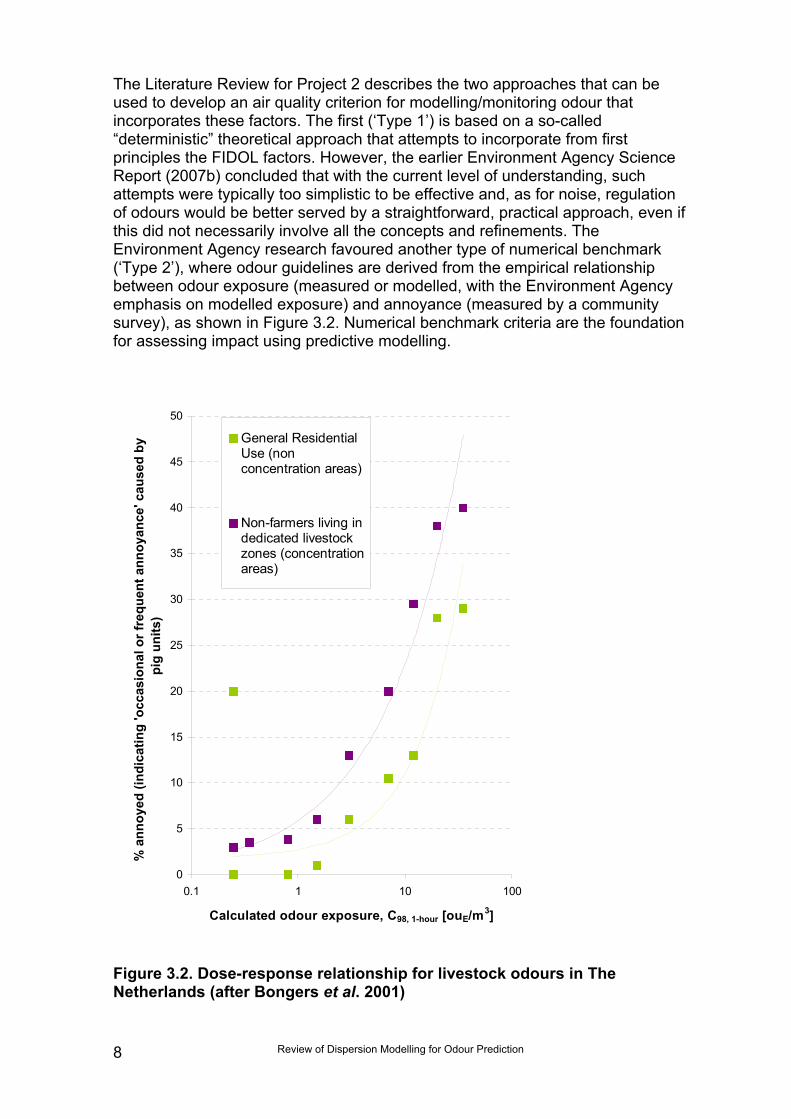
The Literature Review for Project 2 describes the two approaches that can beused to develop an air quality criterion for modelling/monitoring odour thatincorporates these factors. The first (‘Type 1’) is based on a so-called“deterministic” theoretical approach that attempts to incorporate from firstprinciples the FIDOL factors. However, the earlier Environment Agency ScienceReport (2007b) concluded that with the current level of understanding, suchattempts were typically too simplistic to be effective and, as for noise, regulationof odours would be better served by a straightforward, practical approach, even ifthis did not necessarily involve all the concepts and refinements. TheEnvironment Agency research favoured another type of numerical benchmark(‘Type 2’), where odour guidelines are derived from the empirical relationshipbetween odour exposure (measured or modelled, with the Environment Agencyemphasis on modelled exposure) and annoyance (measured by a communitysurvey), as shown in Figure 3.2. Numerical benchmark criteria are the foundationfor assessing impact using predictive modelling.
Figure 3.2. Dose-response relationship for livestock odours in TheNetherlands (after Bongers et al. 2001)
0
5
10
15
20
25
30
35
40
45
50
0.1 1 10 100
Calculated odour exposure, C98, 1-hour [ouE/m3]
% a
nnoy
ed (i
ndic
atin
g 'o
ccas
iona
l or f
requ
ent a
nnoy
ance
' cau
sed
by
pig
units
)
General ResidentialUse (nonconcentration areas)
Non-farmers living indedicated livestockzones (concentrationareas)
Review of Dispersion Modelling for Odour Predictions 9
This led to the Environment Agency developing its numerical benchmarks forodour mixtures that were put forward as “Indicative Odour Exposure Standards”in the Draft H4 guidance.This “Type 2” approach, based on an empirical, epidemiological dose-responsestudy, does not normally concern itself with the details of the FIDOL factors, andinstead treats the process as a “black box”. The overall uncertainty of the DraftH4 method will be a combination of:
• Random component uncertainties – these are precision-type uncertainties,responsible for the scatter and the correlation coefficient found for thedose-response curve; and
• Systematic component uncertainties – these are the bias or accuracy-typeuncertainties that include factors such as how relevant the Dutch pig-odour response curve is to other odour types in UK conditions, and howappropriately the concentration levels for the “offensiveness” bands havebeen set.
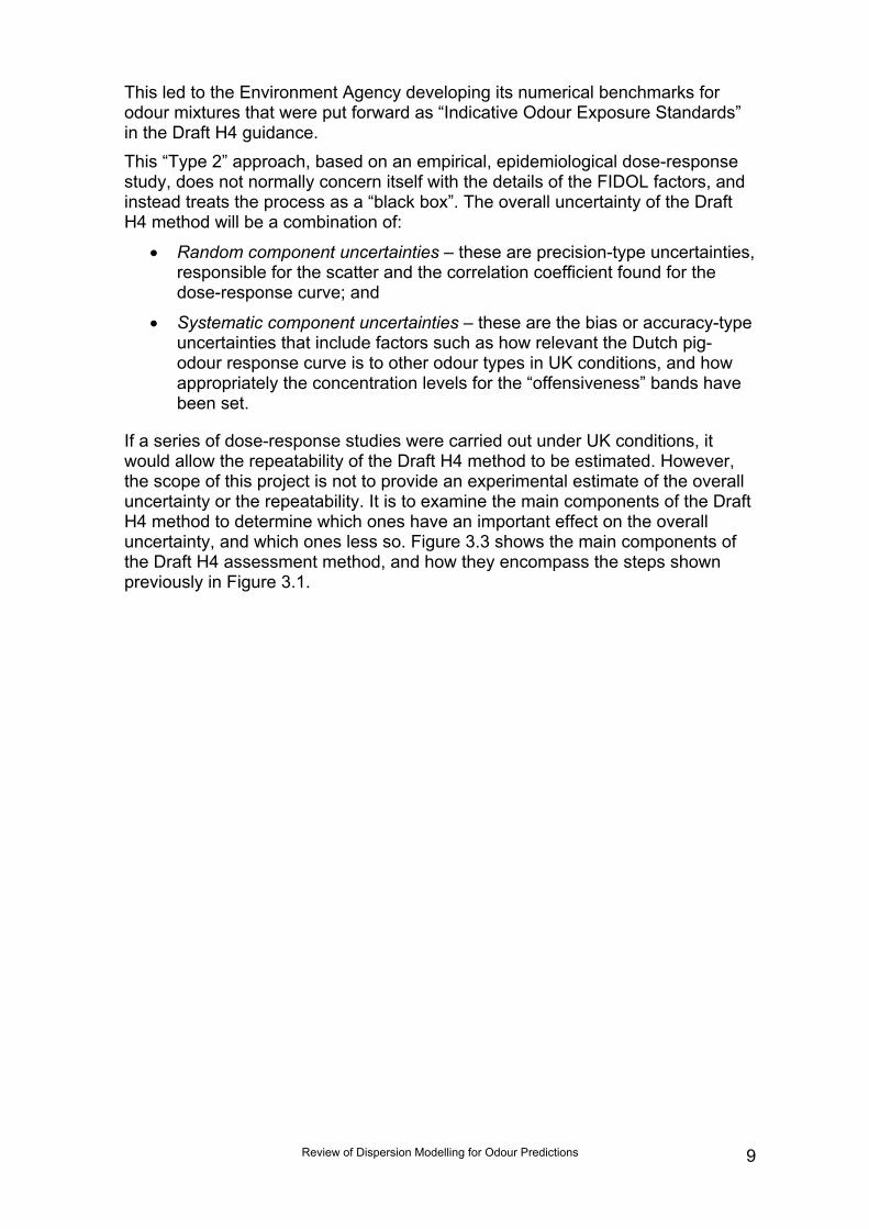
If a series of dose-response studies were carried out under UK conditions, itwould allow the repeatability of the Draft H4 method to be estimated. However,the scope of this project is not to provide an experimental estimate of the overalluncertainty or the repeatability. It is to examine the main components of the DraftH4 method to determine which ones have an important effect on the overalluncertainty, and which ones less so. Figure 3.3 shows the main components ofthe Draft H4 assessment method, and how they encompass the steps shownpreviously in Figure 3.1.
Review of Dispersion Modelling for Odour Prediction10
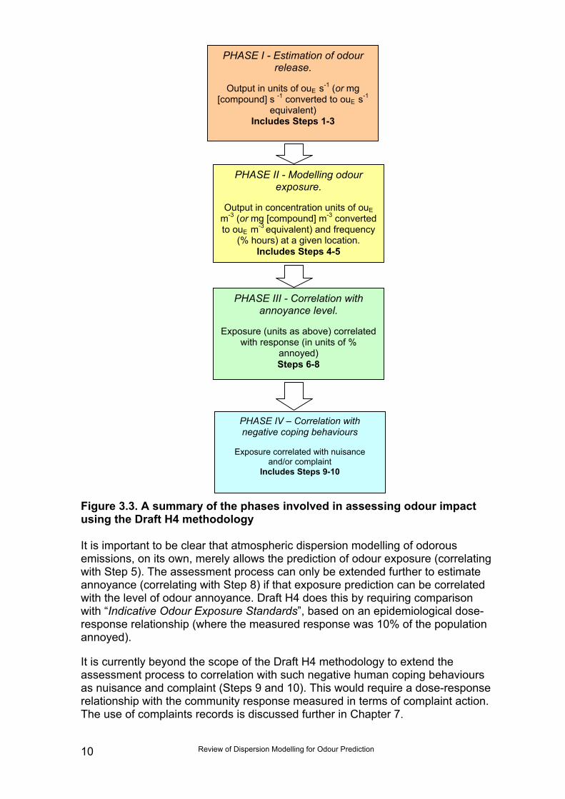
Figure 3.3. A summary of the phases involved in assessing odour impactusing the Draft H4 methodology
It is important to be clear that atmospheric dispersion modelling of odorousemissions, on its own, merely allows the prediction of odour exposure (correlatingwith Step 5). The assessment process can only be extended further to estimateannoyance (correlating with Step 8) if that exposure prediction can be correlatedwith the level of odour annoyance. Draft H4 does this by requiring comparisonwith “Indicative Odour Exposure Standards”, based on an epidemiological dose-response relationship (where the measured response was 10% of the populationannoyed).
It is currently beyond the scope of the Draft H4 methodology to extend theassessment process to correlation with such negative human coping behavioursas nuisance and complaint (Steps 9 and 10). This would require a dose-responserelationship with the community response measured in terms of complaint action.The use of complaints records is discussed further in Chapter 7.
PHASE I - Estimation of odourrelease.
Output in units of ouE s-1 (or mg[compound] s -1 converted to ouE s-1
equivalent)Includes Steps 1-3
PHASE II - Modelling odourexposure.
Output in concentration units of ouEm-3 (or mg [compound] m-3 convertedto ouE m-3 equivalent) and frequency
(% hours) at a given location.Includes Steps 4-5
PHASE III - Correlation withannoyance level.
Exposure (units as above) correlatedwith response (in units of %
annoyed)Steps 6-8
PHASE IV – Correlation withnegative coping behaviours
Exposure correlated with nuisanceand/or complaint
Includes Steps 9-10
Review of Dispersion Modelling for Odour Predictions 11
4 Phase I – Estimation ofOdour Release Value
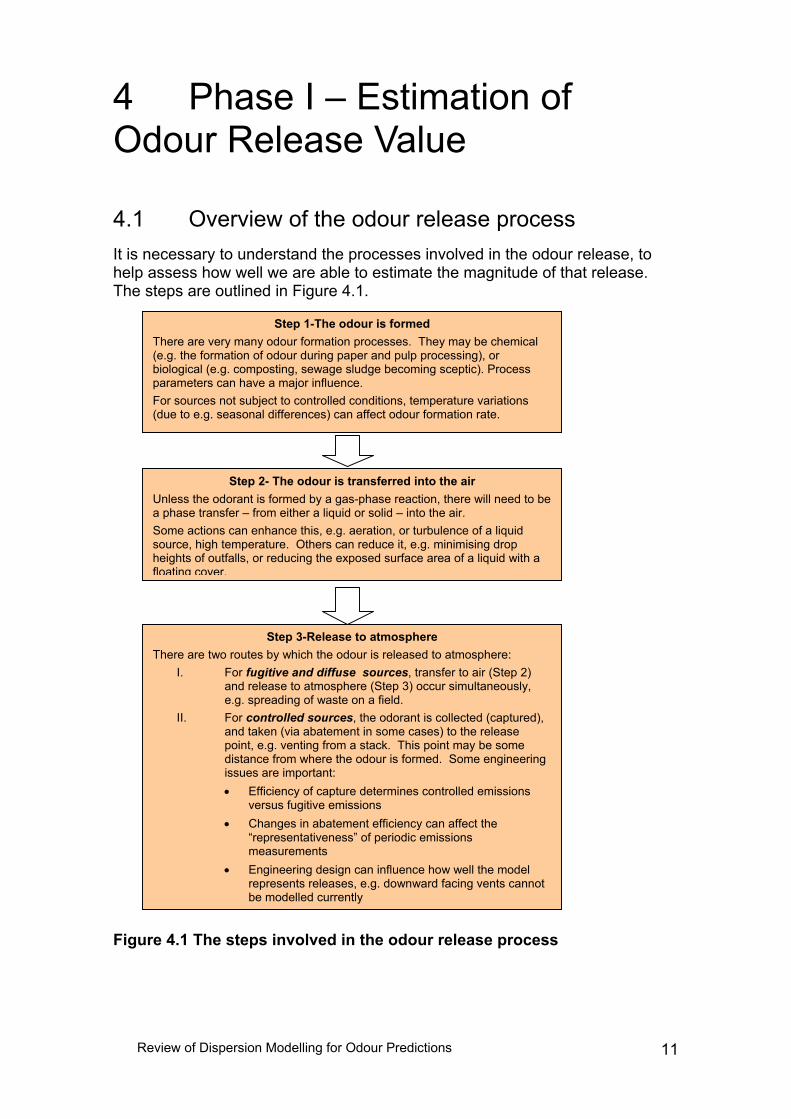
4.1 Overview of the odour release processIt is necessary to understand the processes involved in the odour release, tohelp assess how well we are able to estimate the magnitude of that release.The steps are outlined in Figure 4.1.
Figure 4.1 The steps involved in the odour release process
Step 1-The odour is formedThere are very many odour formation processes. They may be chemical(e.g. the formation of odour during paper and pulp processing), orbiological (e.g. composting, sewage sludge becoming sceptic). Processparameters can have a major influence.For sources not subject to controlled conditions, temperature variations(due to e.g. seasonal differences) can affect odour formation rate.
Step 2- The odour is transferred into the airUnless the odorant is formed by a gas-phase reaction, there will need to bea phase transfer – from either a liquid or solid – into the air.Some actions can enhance this, e.g. aeration, or turbulence of a liquidsource, high temperature. Others can reduce it, e.g. minimising dropheights of outfalls, or reducing the exposed surface area of a liquid with afloating cover.
Step 3-Release to atmosphereThere are two routes by which the odour is released to atmosphere:
I. For fugitive and diffuse sources, transfer to air (Step 2)and release to atmosphere (Step 3) occur simultaneously,e.g. spreading of waste on a field.
II. For controlled sources, the odorant is collected (captured),and taken (via abatement in some cases) to the releasepoint, e.g. venting from a stack. This point may be somedistance from where the odour is formed. Some engineeringissues are important:• Efficiency of capture determines controlled emissions
versus fugitive emissions• Changes in abatement efficiency can affect the
“representativeness” of periodic emissionsmeasurements
• Engineering design can influence how well the modelrepresents releases, e.g. downward facing vents cannotbe modelled currently
Review of Dispersion Modelling for Odour Prediction12
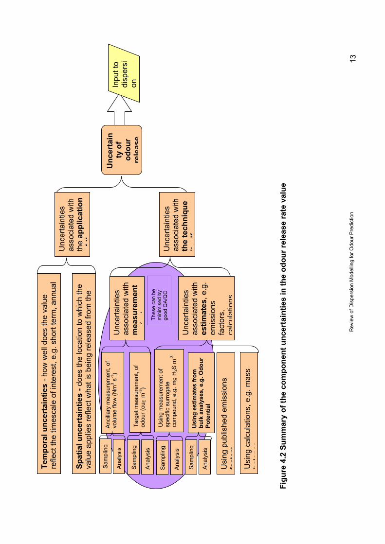
4.2 Summary of the component uncertainties in theodour release rate valueThe component uncertainties that go towards making up the uncertaintyassociated with the odour release value (that is input into the dispersion model)are summarised in Figure 4.2, with further details on these individual uncertaintycomponents given in Section 4.3.
It is crucial to understand that there are many different ways in which the odourrelease value can be obtained. Figure 4.2 attempts to show the choicesavailable to the practitioner. One of the most basic choices is whether the odourrelease rate value will be obtained by measurement, or by estimation (see Box4.1 for clarification of these terms). Both have their place – and are allowed inthe Draft H4 methodology – but as is explained later in this chapter, the choicestaken at this early stage can have big influences on the resulting uncertainty ofthe final odour release value that goes forward into the modelling phase of theassessment.
In looking at Figure 4.2, the first distinction that needs to be made is between:a) the uncertainties associated with the technique itself (whether that be
measurement or estimation); andb) the uncertainties associated with the application of that technique to a
particular scenario/situation.
The next distinction made is that between the two alternative routes to obtainingthe odour release value, namely:I. measurement of the odour release directly: orII. estimation of the odour release.
For an existing installation there may be a choice on whether the release valueswill be based on measurements or estimations. If the installation is not yet inoperation, the releases will need to be estimated. Whichever technique is usedwill have its own component uncertainties.
Rev
iew
of D
ispe
rsio
n M
odel
ling
for O
dour
Pre
dict
ion
13
Figu
re 4
.2 S
umm
ary
of th
e co
mpo
nent
unc
erta
intie
s in
the
odou
r rel
ease
rate
val
ue
Unc
erta
inty
of
odou
rre
leas
e
Usi
ng p
ublis
hed
emis
sion
sfa
ctor
s
Tem
pora
l unc
erta
intie
s - h
ow w
ell d
oes
the
valu
ere
flect
the
times
cale
of i
nter
est,
e.g.
sho
rt te
rm, a
nnua
l
Spat
ial u
ncer
tain
ties
- doe
s th
e lo
catio
n to
whi
ch th
eva
lue
appl
ies
refle
ct w
hat i
s be
ing
rele
ased
from
the
Unc
erta
intie
sas
soci
ated
with
mea
sure
men
tf
d
Unc
erta
intie
sas
soci
ated
with
estim
ates
, e.g
.em
issi
ons
fact
ors,
calc
ulat
ions
Unc
erta
intie
sas
soci
ated
with
the
appl
icat
ion
fth
Unc
erta
intie
sas
soci
ated
with
the
tech
niqu
eits
elf
Targ
et m
easu
rem
ent,
ofod
our (
ouE
m-3
)
Anc
illar
y m
easu
rem
ent,
ofvo
lum
e flo
w (N
m3 s
-1)
Sam
plin
g
Ana
lysi
s
Sam
plin
g
Ana
lysi
s
Usi
ng c
alcu
latio
ns, e
.g. m
ass
bala
nce
Thes
e ca
n be
min
imis
ed b
ygo
od Q
A/Q
C
Inpu
t to
disp
ersi
on
Usi
ng e
stim
ates
from
bulk
ana
lyse
s, e
.g. O
dour
Pote
ntia
l
Usi
ng m
easu
rem
ent o
fsp
ecifi
c su
rrog
ate
com
poun
d, e
.g. m
g H
2S m
-3
Sam
plin
g
Sam
plin
g
Ana
lysi
s
Ana
lysi
s
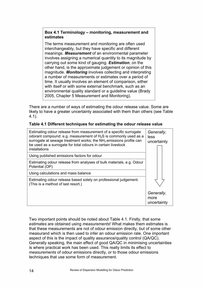
Review of Dispersion Modelling for Odour Prediction14
Box 4.1 Terminology – monitoring, measurement andestimatesThe terms measurement and monitoring are often usedinterchangeably, but they have specific and differentmeanings. Measurement of an environmental parameterinvolves assigning a numerical quantity to its magnitude bycarrying out some kind of gauging. Estimation, on theother hand, is the approximate judgement or opinion of thismagnitude. Monitoring involves collecting and interpretinga number of measurements or estimates over a period oftime. It usually involves an element of comparison, eitherwith itself or with some external benchmark, such as anenvironmental quality standard or a guideline value (Brady2005, Chapter 5 Measurement and Monitoring).
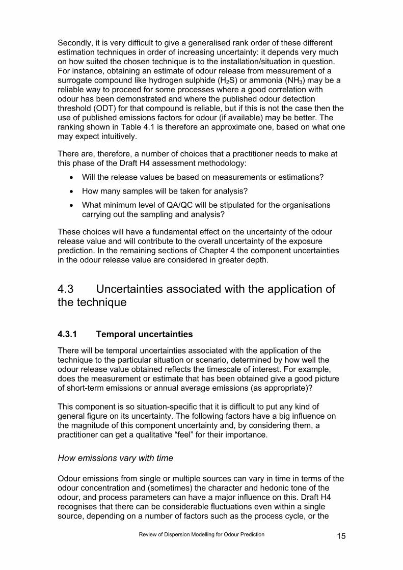
There are a number of ways of estimating the odour release value. Some arelikely to have a greater uncertainty associated with them than others (see Table4.1).
Table 4.1 Different techniques for estimating the odour release value
Estimating odour release from measurement of a specific surrogateodorant compound: e.g. measurement of H2S is commonly used as asurrogate at sewage treatment works; the NH3 emissions profile canbe used as a surrogate for total odours in certain livestockinstallations
Using published emissions factors for odour
Estimating odour release from analyses of bulk materials, e.g. OdourPotential (OP)
Using calculations and mass balance
Estimating odour release based solely on professional judgement.(This is a method of last resort.)
Generally,lessuncertainty
Generally,moreuncertainty
Two important points should be noted about Table 4.1. Firstly, that someestimates are obtained using measurements! What makes them estimates isthat these measurements are not of odour emission directly, but of some othermeasurand which is then used to infer an odour emission rate. One importantaspect of this is the impact of quality assurance/quality control (QA/QC).Generally speaking, the main effect of good QA/QC in minimising uncertaintiesis where practical work has been used. This really limits its effect tomeasurements of odour emissions directly, or to those odour emissionstechniques that use some form of measurement.
Review of Dispersion Modelling for Odour Prediction 15
Secondly, it is very difficult to give a generalised rank order of these differentestimation techniques in order of increasing uncertainty: it depends very muchon how suited the chosen technique is to the installation/situation in question.For instance, obtaining an estimate of odour release from measurement of asurrogate compound like hydrogen sulphide (H2S) or ammonia (NH3) may be areliable way to proceed for some processes where a good correlation withodour has been demonstrated and where the published odour detectionthreshold (ODT) for that compound is reliable, but if this is not the case then theuse of published emissions factors for odour (if available) may be better. Theranking shown in Table 4.1 is therefore an approximate one, based on what onemay expect intuitively.
There are, therefore, a number of choices that a practitioner needs to make atthis phase of the Draft H4 assessment methodology:
• Will the release values be based on measurements or estimations?
• How many samples will be taken for analysis?
• What minimum level of QA/QC will be stipulated for the organisationscarrying out the sampling and analysis?
These choices will have a fundamental effect on the uncertainty of the odourrelease value and will contribute to the overall uncertainty of the exposureprediction. In the remaining sections of Chapter 4 the component uncertaintiesin the odour release value are considered in greater depth.
4.3 Uncertainties associated with the application ofthe technique
4.3.1 Temporal uncertainties
There will be temporal uncertainties associated with the application of thetechnique to the particular situation or scenario, determined by how well theodour release value obtained reflects the timescale of interest. For example,does the measurement or estimate that has been obtained give a good pictureof short-term emissions or annual average emissions (as appropriate)?
This component is so situation-specific that it is difficult to put any kind ofgeneral figure on its uncertainty. The following factors have a big influence onthe magnitude of this component uncertainty and, by considering them, apractitioner can get a qualitative “feel” for their importance.
How emissions vary with time
Odour emissions from single or multiple sources can vary in time in terms of theodour concentration and (sometimes) the character and hedonic tone of theodour, and process parameters can have a major influence on this. Draft H4recognises that there can be considerable fluctuations even within a singlesource, depending on a number of factors such as the process cycle, or the
Review of Dispersion Modelling for Odour Prediction16
weather. The variability of source strength measurements is discussed in somedetail by Best et al. (2004).
Large variations in odour emission rates have been found for agriculturalsources and intensive farming activities (e.g. poultry units), waste watertreatment works and landfill sites. These variations result partly from thebiological sources (e.g. age of birds) and the fact that the processes are notoperating under constant conditions: for example, the moisture content ofpoultry litter increases with the age of the birds, leading to a 5-fold increase inthe odour emission rate. Additional problems are caused by the extendednature of the source and/or the strong meteorological dependence ofdecomposition processes: ambient temperature affects the biological processesand barometric pressure can have a significant influence on emission rates.Open-air sources may be affected by rainfall.
For industrial or water treatment sources, changes in feedstock or productioncycles often dominate, with some well-defined cyclical characteristics but oftenwith quasi-random components. Odour emissions are also often dependent onoperational conditions, which may be difficult to anticipate and controleffectively, for example influent load, changes in the nature of the sewagereceived, frequency of use of open storm tanks, equipment failures,temperature and moisture contents of odorous materials.
Continuous versus periodic monitoring – how well they account fortemporal variations
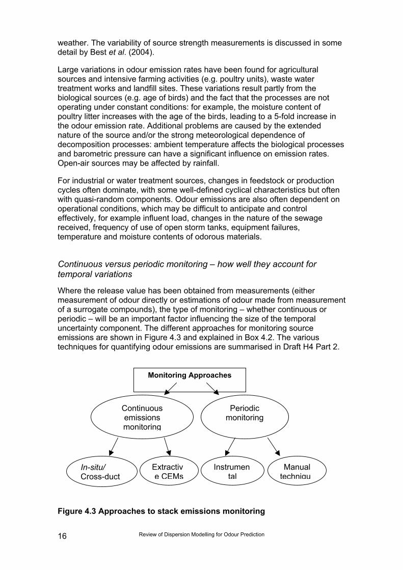
Where the release value has been obtained from measurements (eithermeasurement of odour directly or estimations of odour made from measurementof a surrogate compounds), the type of monitoring – whether continuous orperiodic – will be an important factor influencing the size of the temporaluncertainty component. The different approaches for monitoring sourceemissions are shown in Figure 4.3 and explained in Box 4.2. The varioustechniques for quantifying odour emissions are summarised in Draft H4 Part 2.
Figure 4.3 Approaches to stack emissions monitoring
Monitoring Approaches
Continuousemissionsmonitoring
Periodicmonitoring
In-situ/Cross-duct
Extractive CEMs
Instrumental
Manualtechniqu
Review of Dispersion Modelling for Odour Prediction 17
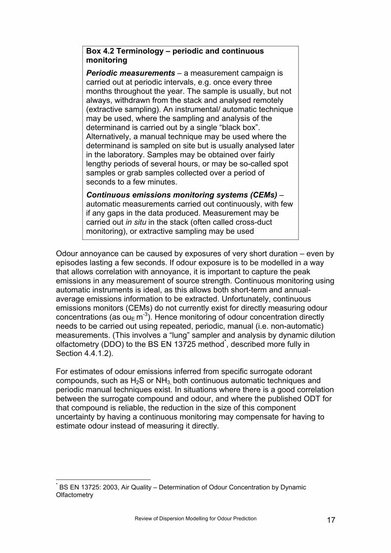
Box 4.2 Terminology – periodic and continuousmonitoringPeriodic measurements – a measurement campaign iscarried out at periodic intervals, e.g. once every threemonths throughout the year. The sample is usually, but notalways, withdrawn from the stack and analysed remotely(extractive sampling). An instrumental/ automatic techniquemay be used, where the sampling and analysis of thedeterminand is carried out by a single “black box”.Alternatively, a manual technique may be used where thedeterminand is sampled on site but is usually analysed laterin the laboratory. Samples may be obtained over fairlylengthy periods of several hours, or may be so-called spotsamples or grab samples collected over a period ofseconds to a few minutes.Continuous emissions monitoring systems (CEMs) –automatic measurements carried out continuously, with fewif any gaps in the data produced. Measurement may becarried out in situ in the stack (often called cross-ductmonitoring), or extractive sampling may be used
Odour annoyance can be caused by exposures of very short duration – even byepisodes lasting a few seconds. If odour exposure is to be modelled in a waythat allows correlation with annoyance, it is important to capture the peakemissions in any measurement of source strength. Continuous monitoring usingautomatic instruments is ideal, as this allows both short-term and annual-average emissions information to be extracted. Unfortunately, continuousemissions monitors (CEMs) do not currently exist for directly measuring odourconcentrations (as ouE m-3). Hence monitoring of odour concentration directlyneeds to be carried out using repeated, periodic, manual (i.e. non-automatic)measurements. (This involves a “lung” sampler and analysis by dynamic dilutionolfactometry (DDO) to the BS EN 13725 method*, described more fully inSection 4.4.1.2).
For estimates of odour emissions inferred from specific surrogate odorantcompounds, such as H2S or NH3, both continuous automatic techniques andperiodic manual techniques exist. In situations where there is a good correlationbetween the surrogate compound and odour, and where the published ODT forthat compound is reliable, the reduction in the size of this componentuncertainty by having a continuous monitoring may compensate for having toestimate odour instead of measuring it directly.
* BS EN 13725: 2003, Air Quality – Determination of Odour Concentration by DynamicOlfactometry
Review of Dispersion Modelling for Odour Prediction18
Periodic monitoring – designing a sampling strategy to minimiseuncertainties from temporal variations
The magnitude of the temporal uncertainties for the application of periodicmonitoring to a particular situation will depend on the number and frequency ofperiodic measurements and their timings in relation to variations in the odouremissions profile of the process. It is not possible to place any numericalestimates of the magnitude of this situation-specific component uncertainty, butpractitioners must make themselves aware of its relative magnitude andimportance. Annexe J (Informative) Sampling Strategy of BS EN 13725 requiresthat these factors should be taken into account.
For odour assessment purposes, the dispersion model requires emissions datawhich are highly-resolved in time and space because odour annoyance can becaused by short-term peaks in odour concentration. Ideally, the data would beresolved over a few seconds (as this is the timescale of individual odour events)but, as noted above, no CEMs currently exist for directly measuring odourconcentrations and we have to rely on periodic measurements. In practicehourly data which take account of diurnal and/or process variations are likely tobe the best available. For existing processes, direct source strengthmeasurements at every different stage of an operating regime is the ideal,including any daily, weekly, production or seasonal cycles. However, odouremission measurements are relatively expensive and currently in the UK theyare rarely carried out with such frequency. If direct source-strengthmeasurements are only practicable for a limited part of the emissions profile,then this should be the point in the cycle when odour emissions are likely to behighest*. Then, the odour emission rate at other points in the cycle could beestimated (with some care) with values below the measurement maximum.
Draft H4 states that worst-case emission scenarios should be considered in anodour assessment. The majority of controlled, point sources (namely those towhich the Draft H4 approach is most applicable) have odour release rates whichare not affected by ambient weather conditions. Even if maximum, worst-caseemissions can be measured/estimated/predicted, the difficulty for predictivemodelling lies in the choice of the prevailing short-term weather conditions foratmospheric dispersion and dilution of the plume that are assumed to coincidewith the peak emission episodes.
Project 1 of this Environment Agency cluster (Environment Agency, 2007a)identified well-defined cycles in emissions from many livestock productionsystems. Bull (2004) investigated the use of different emission scenarios for achicken rearing facility (a constant emission rate over the entire day andincreasing at the end of the 45 day rearing cycle, compared against a scenarioallowing diurnal variations). The AERMOD dispersion model was used for thishypothetical installation. It was found that a constant emission rate gaveunrealistically pessimistic results for the 98th percentile of hourly mean odour
* This point in the emissions cycle may be identified by repeated, sequential measurements ofodour (or some surrogate or indicator), of from a thorough understanding of the process.
Review of Dispersion Modelling for Odour Prediction 19
concentrations. Allowing diurnal variations gave the lowest results, because itcoupled lower emission rates (due to reduced ventilation of the sheds at night)with the worst hourly (stable) meteorological conditions which occur at night.
It is not known whether the historical dose-response modelling studies (forlivestock installations), which formed the basis of the Draft H4 Indicative OdourExposure Standards, took account of emissions variations. No details of themanner in which the odour source data were collated for that study have beenfound to inform Project 3.
The issue of how well the release value obtained reflects actual emissions overthe timescale of interest also applies to release values that are estimated usingmeasurements of specific surrogate compounds (e.g. H2S), emissions factors,analysis of bulk materials (e.g. Odour Potential) and calculations.
4.3.2 Spatial uncertainties
There will be spatial uncertainties associated with the application of thetechnique to the particular situation or scenario, determined by how well theodour release value obtained at the sampling location reflects what is beingreleased from the stack.
Starting first of all at the large-scale spatial issues, it is not uncommon –especially for plant that has been proposed but not yet built – for the odourrelease value to be estimated from measurement (of a odour directly or ofsurrogates) at a representative plant elsewhere. This is combined, if necessary,with factors for scaling up or down. The uncertainty associated with thisapproach depends on just how representative the plant is, and how valid thescaling factors are. Where odour has been estimated from a surrogatecompound (e.g. H2S), there is also the issue of how strong that correlation is forthe site in question. (This is discussed further in 4.4.2.1 for measurement ofspecific compounds.)
There are also spatial issues with the particular process. For quantifying odourreleases from controlled point sources such as stacks, it is preferable to samplethe residual odour emission rate after any abatement system such as scrubber,biofilter, etc. However, there may be situations where the odour release value isobtained before an abatement system. The obvious error is introduced by themeasured concentration itself not reflecting the concentration being releasedfrom the stack, and it would be necessary to correct this figure for theabatement efficiency. This efficiency estimate is itself subject to someuncertainty, which is discussed below. But there is a second possible source oferror that can be introduced by using this approach: the hedonic tone of anodour can be substantially altered by some types of abatement. For example,the odour from a rendering process is generally extremely unpleasant; however,if the same odour has passed through a bio-filter it is much less unpleasant(even at the same odour concentration). Odour abatement techniques aredescribed in a number of documents (Environment Agency, 2002c) includingDraft H4 Part 2, Stuetz and Frechen (2001), and UK WIR Best PracticableMeans Guidebook (2006).
Review of Dispersion Modelling for Odour Prediction20
These issues of how well the release value used reflects actual emissions beingreleased from the stack also apply – to a greater or lesser extent, depending onthe situation - to release values that are estimated using measurements ofspecific surrogate compounds (e.g. H2S), other surrogate measurands,emissions factors, and calculations. For example, when using emissions factorsthese will usually give unit emission rates for the unabated source. This valuewill need to be corrected for the efficiency of any abatement that is used. Thisefficiency value will probably be based on manufacturer’s figures or published,generic abatement efficiencies – if the efficiency was measured by odoursampling then there would not be a need to use emissions factors*. However,such published performance information may not have been based onmeasurements of total odour before and after the abatement, and may bebased on some specific odour compounds only (e.g. H2S). Such efficiencyvalues may not make allowance for the other odorous components in the totalodour of the site in question. Furthermore, the performance characteristics ofcertain abatement techniques depend on ambient temperature. There is,therefore, a need for the practitioner to question the reliability of the publishedabatement efficiencies.
Again, it is not possible to place any numerical estimates of the magnitude ofthese situation-specific uncertainties, but practitioners must make themselvesaware of their possible importance, and form a qualitative view on thesignificance of this component of uncertainty.
4.4 Uncertainties associated with the technique itself
4.4.1 Component uncertainties when measurements of odouremissions are used
4.4.1.1 General overview of uncertainties in source emissionsmeasurements
There are a number of useful sources of information on uncertainty. Generalguidance on uncertainty has been published by the International StandardsOrganisation (ISO 1995), while other guidance from Eurochem (1995) and theRoyal Society of Chemistry (Farrant 1997) addresses uncertainty as applied toanalytical measurements. Several years ago, the Source Testing Association(STA) produced guidance for stack emissions monitoring specifically (Pullen
* Where the abatement efficiency value has been obtained from measurement,the quality of that measurement is important. Ideally odour should have beenmeasured by DDO to method BS EN 13725. The repeatability of thismeasurement is an important consideration: a large number of replicatesimproves the certainty in the measurement. This is discussed in more detail inSection 4.4.1.2.
Review of Dispersion Modelling for Odour Prediction 21
1998). The underlying principles of this guidance remain valid today, and theSTA has reviewed how these main principles should be applied to new andemerging standards and developments and changes in the existing publishedstandards that are used to carry out stack monitoring (Pullen 2003).The main principles of estimating uncertainty in stack monitoring are describedin detail in Appendix A, including calculating uncertainties in practice andcombining component uncertainties to give an estimate of the overalluncertainty. This section focuses on some key points relevant to theidentification of component uncertainties for quantification of odour specifically.Both measurement of the odour emission itself (ouE s-1), and estimation of odouremission from measurement of a specific, surrogate compound (e.g. mgH2S s-1)are described here.Though there are a number of different methods of assessing uncertainty. Thegeneral principle is to use the following process:
i. Specification - define what is being measured and the parameters onwhich it depends;
ii. Identify the sources of uncertainty - for each parameter in therelationship, list the possible sources of uncertainty, e.g. sampling,instrument bias, reagent purity, environmental conditions;
iii. Quantify the uncertainty - measure or estimate, then calculate totaluncertainty using accepted rules.
i. Specification of the measurementQuantification of the odour release from a controlled source involves measuringthe odour concentration and the volume flow of the effluent gas (Equation 4.1):
Equation 4.1Odour release rate Odour concentration Volume flow
ouE s-1
ormg [compound] s-1
= ouE m-3
ormg [compound] m-3
x Nm3 s-1
ii Specification and identification of the sources of uncertaintyThe overall uncertainty that should be considered is that of the wholemeasurement - made up of a sampling stage and an analytical stage*. Thesampling and analysis equipment will be an important, but not the only,component of this. In this conceptual model, measurements using direct-reading instruments (e.g. for H2S) should be treated no differently tomeasurements where a sample is collected discretely and then analysed later
* It is important to not use restrictive definitions of sampling and analysis: in this context theymean the collection of the measured property and its quantification, respectively. Sampling caninclude, for example, the placing of a thermocouple and pitot at a particular point in a stack toobtain the information to calculate the volume flow (necessary to get the mass odour emissionrate from the concentration). The analysis stage in this example is the instrumental conversionof the physical properties to electronic readouts of temperature and pressure.
Review of Dispersion Modelling for Odour Prediction22
(e.g. by DDO) on the laboratory bench. Both have sampling and analysisstages: for example, a flame photometric detector (FPD) analyser forcontinuous monitoring of H2S samples the stack gas through a heated line,conditions the gas (removal of solids and sometimes moisture) and thenpresents it to the reaction cell where the analysis takes place**.
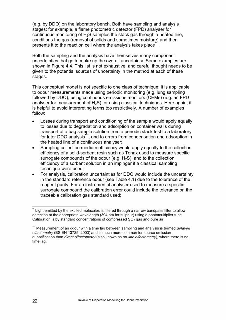
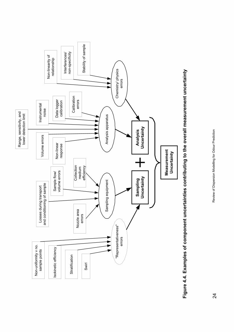
Both the sampling and the analysis have themselves many componentuncertainties that go to make up the overall uncertainty. Some examples areshown in Figure 4.4. This list is not exhaustive, and careful thought needs to begiven to the potential sources of uncertainty in the method at each of thesestages.
This conceptual model is not specific to one class of technique: it is applicableto odour measurements made using periodic monitoring (e.g. lung samplingfollowed by DDO), using continuous emissions monitors (CEMs) (e.g. an FPDanalyser for measurement of H2S), or using classical techniques. Here again, itis helpful to avoid interpreting terms too restrictively. A number of examplesfollow:
• Losses during transport and conditioning of the sample would apply equallyto losses due to degradation and adsorption on container walls duringtransport of a bag sample solution from a periodic stack test to a laboratoryfor later DDO analysis***, and to errors from condensation and adsorption inthe heated line of a continuous analyser;
• Sampling collection medium efficiency would apply equally to the collectionefficiency of a solid-sorbent resin such as Tenax used to measure specificsurrogate compounds of the odour (e.g. H2S), and to the collectionefficiency of a sorbent solution in an impinger if a classical samplingtechnique were used;
• For analysis, calibration uncertainties for DDO would include the uncertaintyin the standard reference odour (see Table 4.1) due to the tolerance of thereagent purity. For an instrumental analyser used to measure a specificsurrogate compound the calibration error could include the tolerance on thetraceable calibration gas standard used;
** Light emitted by the excited molecules is filtered through a narrow bandpass filter to allowdetection at the appropriate wavelength (394 nm for sulphur) using a photomultiplier tube.Calibration is by standard concentrations of compressed SO2 gas and pure air.
*** Measurement of an odour with a time lag between sampling and analysis is termed delayedolfactometry (BS EN 13725: 2003) and is much more common for source emissionquantification than direct olfactometry (also known as on-line olfactometry), where there is notime lag.

Review of Dispersion Modelling for Odour Prediction 23
• Volume errors for DDO analysis would include the tolerance in the dilutionapparatus. For instrumental techniques to measure surrogate compounds itwould include tolerances on reaction-cell volumes, sample-loop volumes,etc. For a classical wet analysis it would include the tolerances on thevolumetric glassware used (e.g. measuring cylinders, pipettes, burettes,etc.).
Rev
iew
of D
ispe
rsio
n M
odel
ling
for O
dour
Pre
dict
ion
24Figu
re 4
.4. E
xam
ples
of c
ompo
nent
unc
erta
intie
s co
ntrib
utin
g to
the
over
all m
easu
rem
ent u
ncer
tain
ty
"Rep
rese
ntat
iven
ess"
erro
rs
Sam
plin
g eq
uipm
ent
Anal
ysis
app
arat
us
Che
mis
try/ p
hysi
cser
rors
Sam
plin
gU
ncer
tain
tyA
naly
sis
Unc
erta
inty
Mea
sure
men
tU
ncer
tain
ty
Non
-uni
form
ity v
no.
sam
ple
poin
ts
Isok
inet
ic e
ffici
ency
Stra
tific
atio
n
Swirl
Loss
es d
urin
g tra
nspo
rtan
d co
nditi
onin
g of
sam
ple
Sam
ple
flow
/vo
lum
e er
rors
Col
lect
ion
med
ium
effic
ienc
y
Noz
zle
area
erro
rs
Ran
ge, s
ensi
tivity
, and
low
er d
etec
tion
limit
Non
-line
arre
spon
se
Inst
rum
enta
lno
ise
Dat
a lo
gger
calib
ratio
n
Cal
ibra
tion
erro
rs
Volu
me
erro
rs
Non
-line
arity
of
rela
tions
hip
Inte
rfere
nces
/no
n-sp
ecifi
city
Stab
ility
of s
ampl
e

Review of Dispersion Modelling for Odour Prediction 25
iii Quantifying the uncertaintiesThere are four main approaches to quantifying the uncertainties, summarised inTable 4.2. Different approaches are appropriate to different situations.Furthermore, some of these approaches give better estimates of uncertaintythan others: the best provide information on the combined effects of thereproducibility of the measurements and the bias (the difference between ameasured value and the “true” value); others give a reasonable estimate of theuncertainty arising from random effects (scatter) but do not address systematic,or bias, uncertainties.
Table 4.2 The four main approaches to quantifying uncertainties in sourceemissions measurementsApproach Advantages DisadvantagesA. Repeat measurements ona certified reference material(CRM)
Gives a “real” value for thewhole uncertainty (i.e. thecombination of precisionand bias)
The accepted reference value for theEuropean odour unit (ouE) is theEuropean Reference Odour Mass(EROM), which is equal to a 123 µg n-butanol evaporated in 1 m3 neutral gas,which produces a concentration of 0.040µmol/mol.Repeat DDO measurements have beencarried out using this standard in thelaboratory, but this only covers theanalysis aspect of the measurement andnot the sampling. A standard referenceodour (or surrogate, e.g. H2S) in the gasstream of a stack is not available, so thisapproach cannot be used currently toquantify the sampling component of themeasurement uncertainty.
B. Experimental work, e.g.repeatability experiments,paired comparisons, and ringtests
Gives a “real” value for theprecision component of theuncertainty
Gives good estimate of precision,repeatability, etc. but often fails toinclude bias.This approach can be expensive, e.g.CEN ring tests up to €100,000 per testwith multiple teams
C. Uncertainty BudgetApproach - estimations basedon previous results/data, e.g.instrument specifications,calibration data, ProficiencyTesting schemes
Can “unpick” theuncertainty budget andrebuild if there arechanges, e.g. deviations,new equipment.
Can appear rather abstract.
D. Estimations based onconsidered judgement
This is usually considered to be the method of last resort
Note: for definitions of terms such as precision, repeatability, reproducibility, accuracy, bias, anduncertainty refer to the definitions given in the CEN standard EN 13725.
As explained in Chapter 1, the purpose of this study is not so much to get aprecise estimate of the overall uncertainty, but rather to investigate the relativeimportance of the main component uncertainties. It would be useful to know, forinstance, if dispersion modelling has a much more significant componentuncertainty than emissions quantification, or assignment to different bands ofunpleasantness. To do this we need to examine separately – quantifying ifpossible – each of the component uncertainties. We then need to see how theycompare. For this, the Uncertainty Budget Approach (C) is relevant.
Review of Dispersion Modelling for Odour Prediction26
4.4.1.2 Uncertainties for direct measurement of odour emissionconcentration (ouE m-3)
The main principles of the measurement
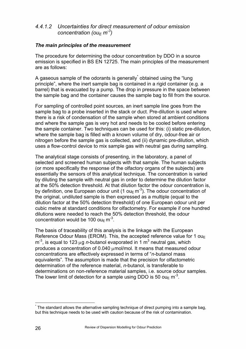
The procedure for determining the odour concentration by DDO in a sourceemission is specified in BS EN 12725. The main principles of the measurementare as follows:
A gaseous sample of the odorants is generally* obtained using the “lungprinciple”, where the inert sample bag is contained in a rigid container (e.g. abarrel) that is evacuated by a pump. The drop in pressure in the space betweenthe sample bag and the container causes the sample bag to fill from the source.
For sampling of controlled point sources, an inert sample line goes from thesample bag to a probe inserted in the stack or duct. Pre-dilution is used wherethere is a risk of condensation of the sample when stored at ambient conditionsand where the sample gas is very hot and needs to be cooled before enteringthe sample container. Two techniques can be used for this: (i) static pre-dilution,where the sample bag is filled with a known volume of dry, odour-free air ornitrogen before the sample gas is collected, and (ii) dynamic pre-dilution, whichuses a flow-control device to mix sample gas with neutral gas during sampling.
The analytical stage consists of presenting, in the laboratory, a panel ofselected and screened human subjects with that sample. The human subjects(or more specifically the response of the olfactory organs of the subjects) areessentially the sensors of this analytical technique. The concentration is variedby diluting the sample with neutral gas in order to determine the dilution factorat the 50% detection threshold. At that dilution factor the odour concentration is,by definition, one European odour unit (1 ouE m-3). The odour concentration ofthe original, undiluted sample is then expressed as a multiple (equal to thedilution factor at the 50% detection threshold) of one European odour unit percubic metre at standard conditions for olfactometry. For example if one hundreddilutions were needed to reach the 50% detection threshold, the odourconcentration would be 100 ouE m-3.
The basis of traceability of this analysis is the linkage with the EuropeanReference Odour Mass (EROM). This, the accepted reference value for 1 ouEm-3, is equal to 123 µg n-butanol evaporated in 1 m3 neutral gas, whichproduces a concentration of 0.040 µmol/mol. It means that measured odourconcentrations are effectively expressed in terms of “n-butanol massequivalents”. The assumption is made that the precision for olfactometricdetermination of the reference material, n-butanol, is transferable todeterminations on non-reference material samples, i.e. source odour samples.The lower limit of detection for a sample using DDO is 50 ouE m-3.
* The standard allows the alternative sampling technique of direct pumping into a sample bag,but this technique needs to be used with caution because of the risk of contamination.
Review of Dispersion Modelling for Odour Prediction 27
The major sources of error in this type of measurement are reported to be thepotential for degradation of the sample after it is collected and the variation inperformance of the odour panellists (Minnesota Pollution Control Agency 2006).
The major component sources of uncertainty in the DDO analysis
The standard contains performance quality requirements for:
• selecting odour panel members with appropriate individual variability andsensitivity;
• calibration of the dilution equipment (the dilution olfactometer) using atracer gas and a physical/chemical method of analysis;
• calibration of the sensor (odour panel) by means of the referenceodorant.
The standard also specifies:
• requirements for construction of the olfactometer and the materials thatcan be used;
• conditioning and cleaning of apparatus;
• the dilution gas and reference material to be used;
• the environmental conditions under which the olfactometry is carried out.
The laboratory should also carry out an overall check on precision by means ofregular performance testing – an inter-laboratory proficiency testing scheme.
The quoted uncertainty (see below) can therefore be considered to include thecomponent uncertainties relating to the above when the olfactory testinglaboratory complies with all the quality criteria specified in the standard.
BS EN 13725 sets several quality performance criteria that the olfactometrylaboratory must comply with, including achieving a certain level of repeatabilityfor the determination of the standard odour. Annexe G (Informative) of thestandard shows how the standard deviation of a population of test results canbe calculated. When the DDO analysis is carried out in full compliance with thestandard, using a properly selected panel and achieving the repeatabilitycriterion in the standard, the 95% confidence interval for one single odourconcentration determination on a sample of 1000 ouE m-3 will be 453 to2209 ouE m-3. Analysing replicate samples can reduce the uncertainty and TableG.1 in Annexe G of the standard shows how this affects the confidence interval.A simplified version of this table is given here (Table 4.3). For a concentrationvalue of 1000 ouE m-3 obtained from two DDO determinations, in 95% of casesthe “true” result will lie in the interval between 571 ouE m-3 and 1752 ouE m-3.The earlier Environment Agency research (2002b) that formed the basis for theDraft H4 approach summarises graphically (shown here as Figure 4.5) theanalysis component of uncertainty that can be expected for a result (nominally1000 ouE m-3) obtained from a given number of replicate DDO determinations.
Review of Dispersion Modelling for Odour Prediction28
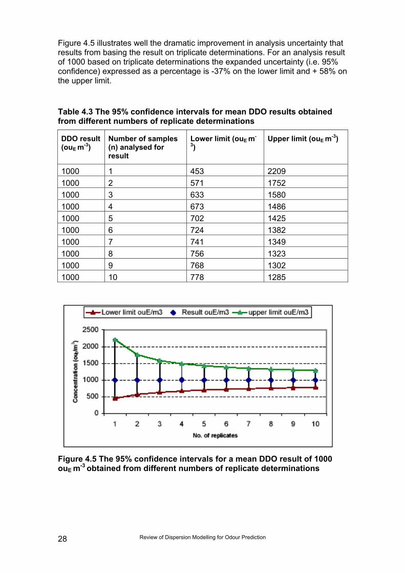
Figure 4.5 illustrates well the dramatic improvement in analysis uncertainty thatresults from basing the result on triplicate determinations. For an analysis resultof 1000 based on triplicate determinations the expanded uncertainty (i.e. 95%confidence) expressed as a percentage is -37% on the lower limit and + 58% onthe upper limit.
Table 4.3 The 95% confidence intervals for mean DDO results obtainedfrom different numbers of replicate determinations
DDO result(ouE m-3)
Number of samples(n) analysed forresult
Lower limit (ouE m-
3)Upper limit (ouE m-3)
1000 1 453 22091000 2 571 17521000 3 633 15801000 4 673 14861000 5 702 14251000 6 724 13821000 7 741 13491000 8 756 13231000 9 768 13021000 10 778 1285
Figure 4.5 The 95% confidence intervals for a mean DDO result of 1000ouE m-3 obtained from different numbers of replicate determinations
Review of Dispersion Modelling for Odour Prediction 29
The major component sources of uncertainty in the sampling of the odour
The previously described component uncertainty for DDO quoted in thestandard are for only the analysis part of the measurement; the uncertaintyvalue doesn’t include the contribution from collecting the stack (or other source)sample. This may be an important contributor to the overall measurementuncertainty.
A major part of the sampling uncertainty will depend on the representivity of thesample collected from the sampling point duct in relation to the bulk effluentgas. If at the sampling location, the bulk gas is well mixed, then these errors willbe minimised. If there is stratified gas flow, then the error can become largeunless multi-point sampling across the duct is employed. The magnitude of thiscomponent uncertainty will be very site-specific and no definitive value can beput on it. However, its significance will be minimised if the sampling location andthe number of sampling points conform to the requirements of the EnvironmentAgency’s M1 guidance (2006) for regulatory compliance monitoring.
A standard reference odour in the gas stream of a stack is not available, so it iscurrently not possible to use the type of approach where the samplingcomponent of the measurement uncertainty is quantified. The standard notesthat further research is needed to characterise the sampling uncertainty, whichwas limited by financial constraints when the standard was developed.Improvements in sampling may be the subject of a future revision of thestandard. It should be noted, however, that BS EN 13725 contains anacceptance limit for “accuracy”* of ≤0.20 for dilution apparatus - both theapparatus used in the olfactometer itself and also when pre-dilution is used insampling to prevent condensation. In the absence of any other estimate for thesampling component uncertainty, this figure of ±0.20 or ±20% has been used asa typical value for sampling.
As well as the collection of the sample, transport and storage between samplingand olfactometry can potentially cause deterioration and losses to the sampleby adsorption, diffusion and chemical transformation. The standard does coversome of these aspects of sampling: performance quality requirements are setfor the materials that can be used in sampling and for conditioning and cleaningof apparatus. The standard notes that experiments so far indicate that lossesbecome significant after 24-30 hours of storage for some substances andtherefore the standard requires that the interval between sampling and analysisshall not exceed 30 hours and the sample shall be kept at >dewpoint<25°C andout of direct sunlight. The assumption is made here that the additional samplinguncertainties due to transport and storage are not significant if theserequirements of the Standard are complied with.
* This was stated as taking into account both bias and random errors, and expressed asrepeatability at 95% confidence limits
Review of Dispersion Modelling for Odour Prediction30
4.4.1.3 Uncertainties for measurement of volume flow (Nm3 s-1)
In order to calculate the odour mass emission rate from the odour concentrationmeasurement, it is necessary to know the volume flow.Annex I (Informative) of BS EN 13725 quotes method ISO 9096* for measuringthe flow rate in the duct, with the volume flow rate then calculated at ‘Standard’conditions (293 K, 101.3 kPa) for wet conditions following ISO 10780**.However, atmospheric dispersion models require the volume flow at Normalconditions (273 K, 101.3 kPa) rather than Standard conditions. This is obtainedfrom the following equation:Equation 4.2Volumeflow
Gas streamvelocity
Duct crosssectionalarea
Temperaturecorrection
Pressurecorrection
Nm3 s-1
=
m s-1
x
m2
x
273/Temp(K)
x
Pressure(kPa)/101.3
The actual measurands to obtain these factors are:
• Pitot pressure (kPa), calibrated against velocity;
• Duct diameter, or breadth and depth (m); and
• Thermocouple output (mV) calibrated against temperature (K).
• Pitot pressure (Pa), giving absolute pressure in the stack.Each of these has their own component uncertainties.Hawksley et al (1997) studied measurements of particulates to BS3405.Although this standard is now withdrawn, the flow measurement aspect is littledifferent from the more recent standards. Using the flow estimate to calculatethe particulate concentration from the particulate emission rate was said toincrease the uncertainty by a √2 factor.
As part of its MCERTS accreditation, Bureau Veritas’ emissions monitoringteam has calculated the uncertainty of gas flow rate measurements using pitotstatic tubes for a typical stack of duct diameter 1 m and gas velocity of 15 m s-1
(Bureau Veritas 2005). Based on an uncertainty budget built up from thecomponent uncertainties of velocity measurement and linear dimensionmeasurement, the standard uncertainty is about ±5.7% of the calculated value,and the expanded uncertainty at 95% confidence limits (i.e. x 1.96) is about±11%. This does not include uncertainties introduced by conversion of thevolumetric flow-rate at duct conditions (of temperature and pressure) to
* ISO 9096, Stationary source emissions – determination of concentration and mass flow rate ofparticulate material in gas-carrying ducts – Manual gravimetric method.
** ISO 10780, Stationary source emissions – Measurement of velocity and volume flow-rate ofgas streams in ducts.
Review of Dispersion Modelling for Odour Prediction 31
reference conditions. Bureau Veritas calculates that the temperaturemeasurement typically has an expanded uncertainty of ±5%. Taking the squareroot of the sum of the squares of these component uncertainties gives acombined standard uncertainty of ±6.2%, or an expanded uncertainty of ±12%.This assumes the sampling location and stack gas flow stability meets therequirements of the Environment Agency’s M1 guidance for regulatorycompliance monitoring. This also enables the uncertainty due to themeasurement of volume flow (which is an input to the dispersion model) to beranked relative to other component uncertainties for Phase II (see Figure 5.2).The component uncertainty for flow measurement also applies to estimates ofodour releases that have been obtained from measurements of specific,surrogate compounds (Section 4.4.2.1). Emissions factors and mass flowcalculations (Sections 4.4.2.2 and 4.4.2.4, respectively) usually requireknowledge of flow as well.
4.4.1.4 Minimisation of measurement uncertainties by effective QA/QC
High standards of QA/QC are essential in measurements of odour emissionrates. When an emission rate is used in dispersion modelling, any error in theemission rate will transfer directly to an error in the predicted 98th percentileground level odour concentration. Sampling and analysis should be inaccordance with accredited procedures, for which error margins have beenassigned.
At a general level, all emissions measurements submitted to the EnvironmentAgency for regulatory compliance purposes must be covered by theEnvironment Agency-sponsored MCERTS quality scheme (see Box 4.3).
Organisations and individuals carrying out the measurements must holdMCERTS certification and qualifications, respectively. The organisation mustmeet the requirements of EN ISO/IEC 17025 for the MCERTS PerformanceStandard for Organisations. This provides a robust framework for the quality ofthe measurements and helps ensure uncertainties are minimised.At a method-specific level, BS EN 13725 contains numerous QA/QCrequirements to ensure that the testing laboratory produces olfactometry resultswithin the quoted uncertainty for the DDO method.The use of QA/QC to minimise uncertainties applies not only to DDOmeasurements but also to estimates of odour releases that have been obtainedfrom measurements of specific, surrogate compounds (Section 4.4.2.1). Again,
Box 4.3 MCERTSThe Agency’s Monitoring Certification Scheme (MCERTS), launched in 1998,focused initially on type approval of continuous monitoring systems (CEMs)for stacks. The Agency has broadened the scheme to cover periodicmeasurements using portable equipment, termed manual stack-emissionsmonitoring. Because the quality of such periodic measurements depend notonly on the equipment, but also on the competence of the individual and theorganisation, MCERTS for manual stack monitoring covers both these areas.
Review of Dispersion Modelling for Odour Prediction32
MCERTS should apply where the measurements are for regulatory compliancepurposes.
4.4.1.5 Comment on odour measurement uncertainties for diffuse andfugitive sources
Diffuse sourcesAlthough emission rates of area sources (both solid and liquid) can bemeasured, ELVs have not been widely used for compliance checking purposes(although measurement is sometimes used for impact assessment). As suchreleases are not usually controlled sources, they generally cannot be operatedin such a way as to remain below an imposed ELV; instead these sources tendto be managed by indicative/generic Best Available Techniques (BAT)standards to minimise releases. As the Draft H4 approach is used mainly inPPC applications to back-calculate an acceptable ELV for day-to-day sourcecontrol from the ambient odour benchmark, it finds little application in regulatorycompliance of diffuse sources.
Nevertheless, for completeness, some comments on the measurementuncertainties for diffuse sources are given here. It is possible to measure theemission from area sources such as open tanks, but only if the surface ishomogeneous. The analytical stage, involving DDO, is common for any sourceodour sample; however, significant differences exist between the techniques forcollecting samples from diffuse sources compared to point sources. Gostelow(2000) describes the special techniques (e.g. micrometeorological method, fluxhoods) to estimate odour emission rates from area sources but points out thatfurther work is required to validate many odour formation predictioncalculations. BS EN 13725 describes how area sources are sampled: instead ofusing an inert sample line to a probe in a stack, the sampling line goes to asampling hood which is placed over, or floated on, a defined surface area of thesource (e.g. landfill surface, effluent lagoon, etc.). The hood is ventilated withodour-free air at a known volumetric flow rate. The velocity of this ventilation airacross the sampled area of the source affects the rate of odour emission fromthe source, and must therefore be noted. This arrangement is known as a “fluxhood” and several types exist with considerable variation in design. Onecommon type is the Lindvall hood, but the standard points out that this wasoriginally designed only for making comparative measurements of transfer ratesfrom surfaces; there is a need for standardisation and a re-assessment of theunderlying physical assumptions, including whether the flow pattern simulatedunder the hood is representative of real conditions (as is commonly assumed).In particular, the air velocity used is often well below typical wind velocities.There is also the potential that interaction with the matrix (e.g. shading of thesource/protection from the wind etc.) could alter evaporation. The standardstates that further research and validation is required.No details have been found on how these limitations translate into numericalsampling uncertainties. However, it is reasonable to assume that sampling ofodour from a diffuse release such as an area source has a greater level ofuncertainty than for a controlled point source (e.g. stack) release. The reasonsfor this are:
Review of Dispersion Modelling for Odour Prediction 33
• Sampling of odour emissions are far easier for stacks than for areasources;
• Sampling of odour emissions from stacks is more representative of realconditions than sampling from area sources;
• Area sources are inherently more prone to emissions variability e.g.seasonal variability for lagoons at waste water treatment facilities.
Fugitive sourcesFugitive emissions can occur from plant, buildings, tanks and vessels. Fugitiveodour events are often a result of infrequent operations (such as cleaning ormaintenance) or continuous releases (such as leaks from valves and pumps ata refinery) which produce high levels of odour yet cannot be quantified ormeasured. Examples of fugitive emissions or those which cannot be readilymeasured are:
• Raw material or waste storage and handling;
• Transfer processes (e.g. unloading of vehicles at waste transfer site);
• Washing, cleaning and maintenance operations;
• Start-up and shut-down;
• Emergency releases or leaks;
• Pumps and flanges;
• Formation of odorous by-products;
• Contaminated or blocked drains.
BS EN 13725 states clearly in Annexe J (Informative) Sampling Strategy, thatquantifying fugitive emissions incurs large errors and no known samplingtechnique can be recommended. No figures are given, but it is reasonable todeduce from this that they are in orders of magnitude. Draft H4 recognises thatfugitive emissions are difficult to measure/predict, and their modelling in mostcases is inappropriate. Fugitive emissions are better controlled throughimproved housekeeping/containment and by indicative/generic BAT, than byapplication of the modelling/back-calculation approach.
Other acute odour emissions that can be considered objectionable or offensiveon a single occasion are often associated with abnormal or upset conditions.Examples are malfunctioning abatement systems, or infrequent activities suchas re-opening old areas of fill at landfill. Such highly variable and/or uncontrolleddischarges are typically very difficult to quantify and as such are not amenableto the Draft H4 predictive approach.
Again, there are no details on how these limitations translate into numericalsampling uncertainties. However, bearing in mind the above comments andrecommendations it is reasonable to assume that sampling of odour from afugitive release would have a significantly greater level of uncertainty than foreither a controlled point source (e.g. stack) release or a diffuse release such asan area source.
Review of Dispersion Modelling for Odour Prediction34
4.4.2 Component uncertainties when estimates of odouremissions are used
4.4.2.1 Uncertainties from odour release estimates derived frommeasurement of specific compound concentrations (mg m-3)
Application of this approachIt is possible to estimate the odour release value from measurement of asurrogate compound that is correlated well with odour. The use of odourdetection threshold (ODT) values for specific chemical species to effect aconversion from the concentration of the compound (mg m-3) to an equivalentodour concentration (ouE m-3) is described in Draft H4. The equivalent odourconcentration is then multiplied by the volume flow of the release to give theequivalent odour emission rate (ou s-1).This approach has been used at sewage treatment works and for intensivepoultry farming emissions, where popular surrogates for odour have been H2Sand NH3, respectively.There are three aspects to the uncertainty in estimating odour emissions fromspecific compounds:
• What is the uncertainty in the measurement (sampling plus analysis) ofthe surrogate compound?
• How well does the specific compound account for the total odour at thesite in question? This was discussed briefly in Section 4.3.2.
• How robust is the conversion from the concentration of the compound(mg m-3) to an equivalent odour concentration (ouE m-3) using the ODT?
Uncertainty in the measurement of the surrogate compoundThe Environment Agency’s M2 guidance (2004) lists the monitoring techniquesand published methods that are acceptable under MCERTS for regulatorycompliance checking of controlled point-source emissions to air. For H2S andNH3, both continuous automatic techniques and periodic manual techniquesexist, operating on a variety of analytical principles such as uv and ir-spectrometry, chemiluminescence, continuously-sampling chromatography,FPD, and electrochemical cells. For some diffuse sources, continuousautomatic techniques can also be used: in Project 1 of this cluster (EnvironmentAgency 2007a), Silsoe Research Institute describes techniques it hasdeveloped to monitor continuously the emissions ammonia from agriculturalbuildings. In situations where there is a good correlation between the surrogatecompound and odour, the reduction in the size of this component uncertainty byhaving a continuous monitoring may compensate for having to estimate odourinstead of measuring it directly.
The measurement uncertainty for each of these techniques and methods will besomewhat different (and this information is not listed in M2). All MCERTS-accredited organisations carrying out such measurements for regulatorycompliance purposes are obliged to quote the measurement uncertainties,incorporating sampling and analysis. For modern instrumental techniques the
Review of Dispersion Modelling for Odour Prediction 35
expanded (i.e. 95% confidence level) uncertainty of concentrationmeasurements is usually within ±10% (expressed as a percentage of themeasured range).
This is consistent with values quoted by Yang and Hobson (2000) who reviewedtechniques for estimating emission rates of H2S from point sources, from areasources (channels, weirs and open tanks) at waste water treatment works usinga flux chamber, and from estimations based on the theory of gas-liquid transfer.The error associated with the determination of odour emission rate for a pointsource was said to be typically around +3–10% for H2S if the measurement ofairflow is accurate. The authors recognised that little is known about theaccuracy of indirect methods for estimating odour emission rates. This studyalso stated that odour emission rates from enclosed processes could vary byover two orders of magnitude depending on the condition of the flow.
How well the specific compound accounts for total odour at the siteThe specific compound(s) should be responsible for the vast majority of theodour in the emissions, or at least be considered as an empirical surrogate forthe odour.
Although there is no absolute consensus on how odour should be quantified atwastewater treatment works, hydrogen sulphide is commonly used as asurrogate for odour due to its ease of monitoring. This technique isacknowledged in the draft Defra guidance (2004) on odour from sewagetreatment works. The main limitation of this approach is that one chemicalcompound cannot always accurately and consistently represent the overallodour effect of a mixture of compounds. For example, odour monitoring studiesat some sewage treatment works have shown H2S to be a poorer indicator ofsewage treatment odours than is commonly assumed. Whilst it is true that H2Smay be a major component of the sewage treatment works odour cocktail, thisdoes not allow for the complex organic odours associated with sewage andthere are other odorous compounds which may be present and may contributeto the odour impact. Sometimes, a high correlation is found between ambientodour (ouE m-3) and H2S mass emission rate. On the other hand, one study(Fraser 2004) showed that measured H2S in liquor samples from preliminarytanks at a waste water treatment works was less than 5% of total odour, whichwould suggest that under these circumstances H2S may not be used as a proxyat low levels of odour. Other studies (Stuetz & Frechen, 2001) showed that H2Swas a good surrogate indicator for some aspects of the sewage treatmentprocess, namely sludge storage and handling, and preliminary treatment beforeodour control, where it is the dominant odorant. Poorer correlation was foundwhen lime dosing is employed, after odour control (which may remove H2Spreferentially to other odorants), for secondary treatment odours/aeration tankodours (which should not generate H2S unless overloaded), for industrialeffluents, and for dryers/incinerators. H2S is proportionally less important as anodorous component in these sources. It is theoretically possible to use thesecorrelations predict odour concentrations from H2S concentrations but thiswould require detailed knowledge of the processes and conditions at the works.
Similarly, other studies (Freeman et al. 2000) have found that hydrogensulphide and methane (CH4) concentrations in samples of landfill gas did not
Review of Dispersion Modelling for Odour Prediction36
correlate well with odour concentration, suggesting that other compounds in thelandfill gas were also contributing to the odour nuisance.
It is noteworthy that the Western Australian EPA (Department of EnvironmentProtection 2002) allows the geometric mean air odour threshold to be used formodelling odour impacts only when a single odorant in an air stream is presentand there are appropriately reviewed odour thresholds for the odorant available,giving as an example those from the US EPA (1992).
It is not possible to place any generally applicable numerical estimates of thecomponent uncertainty from how well the specific compound accounts for thetotal odour at the site in question. This component uncertainty is site andsituation-specific. Practitioners must make themselves aware of the possibleimportance and form a qualitative view on the significance of this component ofuncertainty.
The robustness of the conversion from the compound concentration to anequivalent odour concentration using the ODTEven if the surrogate compound is responsible for the vast majority of the odourin the emissions, monitoring of individual compounds is still an imperfect way ofquantifying odour releases due to the following:1. This approach assumes the relationship between gas concentration and
odour concentration to be linear, which is not always the case.2. An odorous gas can comprise a cocktail of many odorous compounds
and this approach does not work well for mixtures. Firstly, it is difficult toidentify all the odorous compounds. Secondly, the overall odourconcentration of a mixture cannot be estimated by simply adding thevalues of the chemical constituents. This may give an overestimate or anunderestimate because there may be non-linear additive or synergisticeffects between the various compounds and due to the way that odourstimuli are processed by the human brain.
3. Published odour threshold data may be contradictory and of varyingquality. This is due to differences in olfactometry analytical techniquesused by laboratories in the past (although this became morestandardised from the late 1990s), and also to the use of differentdefinitions of the odour threshold, such as detection, certainty andrecognition levels. More details on this are given in the Literature Reviewfor Project 2, which is part of this cluster (Environment Agency 2007b).
The component uncertainty from the conversion from the mg m-3 to anequivalent ouE m-3 using the ODT depends on the quality of data available forthe particular compound. Older data may be less precise and may also containsignificant bias, so it is important that practitioners use, wherever possible, up-to-date threshold data obtained using a validated standard method (especiallyBS EN 13725) to keep this uncertainty to a minimum. Where ODTs have beenobtained using DDO carried out to BS EN 13725 then the analysis uncertaintyquoted in Section 4.4.1.2 should apply. For example, for an ODT result obtainedfrom triplicate determinations the expanded uncertainty (i.e. 95% confidence)expressed as a percentage is -37% on the lower limit and + 58% on the upperlimit.
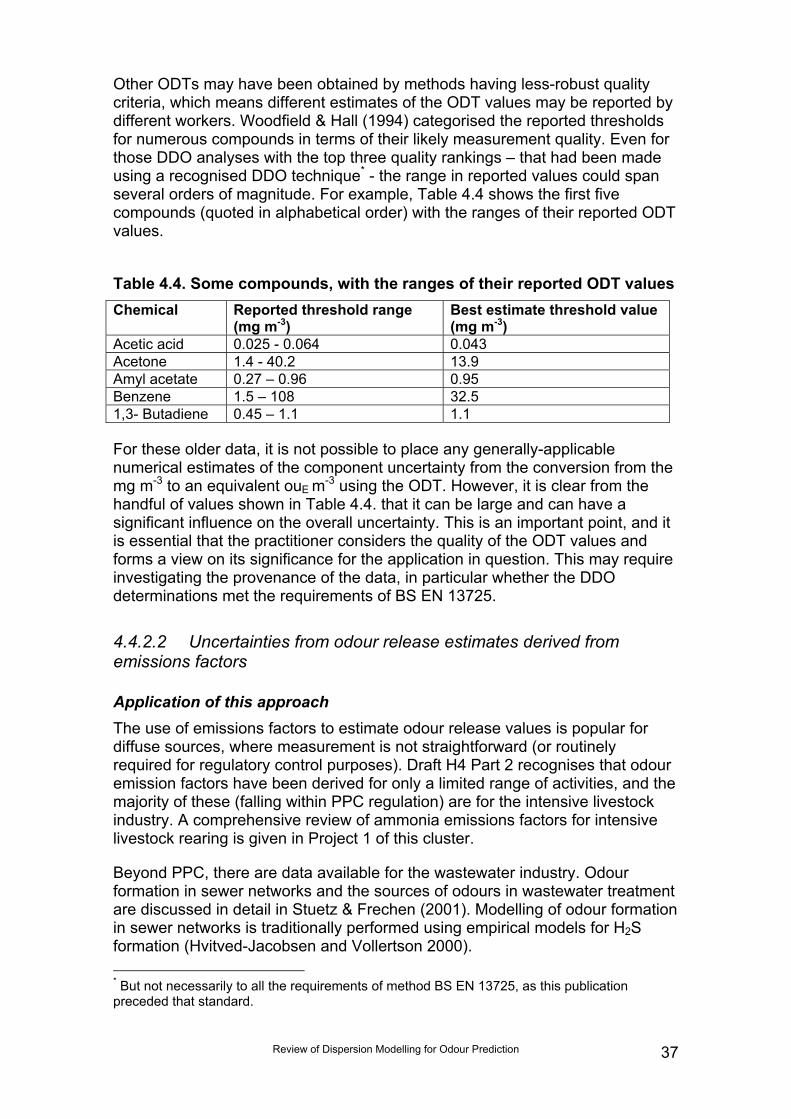
Review of Dispersion Modelling for Odour Prediction 37
Other ODTs may have been obtained by methods having less-robust qualitycriteria, which means different estimates of the ODT values may be reported bydifferent workers. Woodfield & Hall (1994) categorised the reported thresholdsfor numerous compounds in terms of their likely measurement quality. Even forthose DDO analyses with the top three quality rankings – that had been madeusing a recognised DDO technique* - the range in reported values could spanseveral orders of magnitude. For example, Table 4.4 shows the first fivecompounds (quoted in alphabetical order) with the ranges of their reported ODTvalues.
Table 4.4. Some compounds, with the ranges of their reported ODT valuesChemical Reported threshold range
(mg m-3)Best estimate threshold value(mg m-3)
Acetic acid 0.025 - 0.064 0.043Acetone 1.4 - 40.2 13.9Amyl acetate 0.27 – 0.96 0.95Benzene 1.5 – 108 32.51,3- Butadiene 0.45 – 1.1 1.1
For these older data, it is not possible to place any generally-applicablenumerical estimates of the component uncertainty from the conversion from themg m-3 to an equivalent ouE m-3 using the ODT. However, it is clear from thehandful of values shown in Table 4.4. that it can be large and can have asignificant influence on the overall uncertainty. This is an important point, and itis essential that the practitioner considers the quality of the ODT values andforms a view on its significance for the application in question. This may requireinvestigating the provenance of the data, in particular whether the DDOdeterminations met the requirements of BS EN 13725.
4.4.2.2 Uncertainties from odour release estimates derived fromemissions factors
Application of this approachThe use of emissions factors to estimate odour release values is popular fordiffuse sources, where measurement is not straightforward (or routinelyrequired for regulatory control purposes). Draft H4 Part 2 recognises that odouremission factors have been derived for only a limited range of activities, and themajority of these (falling within PPC regulation) are for the intensive livestockindustry. A comprehensive review of ammonia emissions factors for intensivelivestock rearing is given in Project 1 of this cluster.
Beyond PPC, there are data available for the wastewater industry. Odourformation in sewer networks and the sources of odours in wastewater treatmentare discussed in detail in Stuetz & Frechen (2001). Modelling of odour formationin sewer networks is traditionally performed using empirical models for H2Sformation (Hvitved-Jacobsen and Vollertson 2000). * But not necessarily to all the requirements of method BS EN 13725, as this publicationpreceded that standard.
Review of Dispersion Modelling for Odour Prediction38
Currently, there is no openly available database on odour emission factorsacross industry types specific to the UK. Many industries or companies holdinformation on emission rates for their own processes, much of it subject tocommercial confidentiality and not representative across a spectrum ofoperating conditions or weather patterns.
There is a need to improve the accessibility, robustness and use of datapertaining to odour emission rate estimates. An analogy may be made with theDefra Emission Factor Database (EFD) for the Air Quality Strategy prioritypollutants. This is a centralised source of emission estimates for differentprocesses, with quality ratings and/or traceability of the source of the estimates.
A tool/resource such as this is in place in Germany (Lohmeyer et al. 2004a),funded by the State of Baden-Wurttemberg Ministry of the Environment andTransport. GERDA is a computer database which contains a bank of emissionfactors (covering biological solid waste composting plants, repair paint shops,smokehouses, sewage treatment plants and foundries). The spreadsheetcontains procedures to estimate odour emission rates for each part of a site,taking account of factors such as meteorology and operating conditions.GERDA is stated to be a screening tool, which would imply that more site-specific emission factors may be required for detailed assessment.
Uncertainty in the emissions factorsThere are two aspects to the uncertainty associated with an emissions factor.There are the component uncertainties from the unit odour release rate (e.g. foran area release X ouE m-2 s-1) and from the scaling factor (e.g. temperature,number of pigs or birds, throughput tonnage or volume, etc.)
The accuracy of the scaling factor and its applicability to the site/situation inquestion is an issue of “portability” of the emission factor (i.e. how applicable isit to the scenario in question) and this was covered in Sections 4.3.1 and 4.3.2.Here we are only concerned with the uncertainty of the unit emissions factoritself. It is clearly important: according to Yang and Hobson (2000), odouremission rates from sewage treatment works can vary by over two orders ofmagnitude for a given process depending on the condition of the flow.
Emissions factors mass balance calculations are applied most commonly todiffuse sources and fugitive sources that are difficult to monitor. The Draft H4approach - using modelling to back-calculate permissible ELVs - is notapplicable to emissions factors and only limited comments have been made forthe sake of completeness as it is recognised that the Environment Agency will,from time to time, receive EIAs that include odour impact predictions usingemissions factors.
Bull (2004) compared Environment Agency emissions factors (EnvironmentAgency 2003) for intensive poultry rearing with other published values and withmeasurements and found differences of up to an order of magnitude. Similar, ifnot greater variations were said to exist for published odour emissions rates forlandfill sites and wastewater treatment plant.
The wastewater industry has also published some odour emission rates (WRc1998). Yang and Hobson (2000) have suggested that the literature values of
Review of Dispersion Modelling for Odour Prediction 39
odour emission rates have an uncertainty in the region of two orders ofmagnitude or more, because the degree of septicity as measured by the odourpotential or sulphide concentration is never stated, nor are the precise details ofthe process stated (e.g. emission rates from a weir are proportional to the weirheight). Their view was that establishing credible emission rates is potentiallythe weakest link by far in the quantitative assessment of odour impacts.
In searching for published values of odour emission factors, care should betaken that the emission rates have been obtained using the same standards ofdynamic olfactometry. In the UK, the Draft H4 benchmarks are expressed interms of European odour units (ouE). Australia has recently developed jointlywith New Zealand its own standard for odour measurement, which has used theCEN draft EN13725 as a starting point. Prior to this, the different states inAustralia used very individual approaches to odour measurement, and crudeconversion factors between the odour units as defined by various states and theouE are available (Environmental Protection Authority New South Wales 1995).Particularly noteworthy is that 2 ouE m-3 according to the Dutch NVN2820standard is equivalent to 1 ouE m-3 according to CEN draft EN13725.
As with measurement, the emission factor can be of odour itself, or it can be ofa specific compound(s) which can then be converted to odour-equivalents usingpublished ODT values. For example, the US EPA method for estimating loadinglosses of gasoline vapours at oil refineries using emissions factors has a quoteduncertainty of ±30% (for predicting total VOCs). To this needs to be added theuncertainty associated with using a surrogate compound (covered previously inSection 4.2.2.1).
4.4.2.3 Uncertainties from odour release estimates derived fromanalyses of bulk materials
Liquor from open tanks may be sampled and the Odour Potential (OP)measured using published WRc methods. WRc has developed a SewageTreatment Odour Prediction (STOP) model (Yang and Hobson 1998). TheSTOP model takes the odour potential of the waste and the physicalparameters of the process unit to estimate odour emissions. Similarly, theCH2M HILL Interceptor Odor Model can be used to estimate liquid and vapourphase H2S concentrations at various locations throughout the sewage collectionsystem and waste water treatment plant (Witherspoon et al. 2000).
It is not known, however, if any uncertainty estimates/margins of error areassigned to the outputs of these emissions models. In any case, theseapproaches do not really fall within the intended application of the Draft H4,using modelling to back-calculate permissible ELVs.
4.4.2.4 Uncertainties from odour release estimates derived fromcalculations
However, for the sake of completeness we have included some limitedcomments on other sources, as it is recognised that the Environment Agency
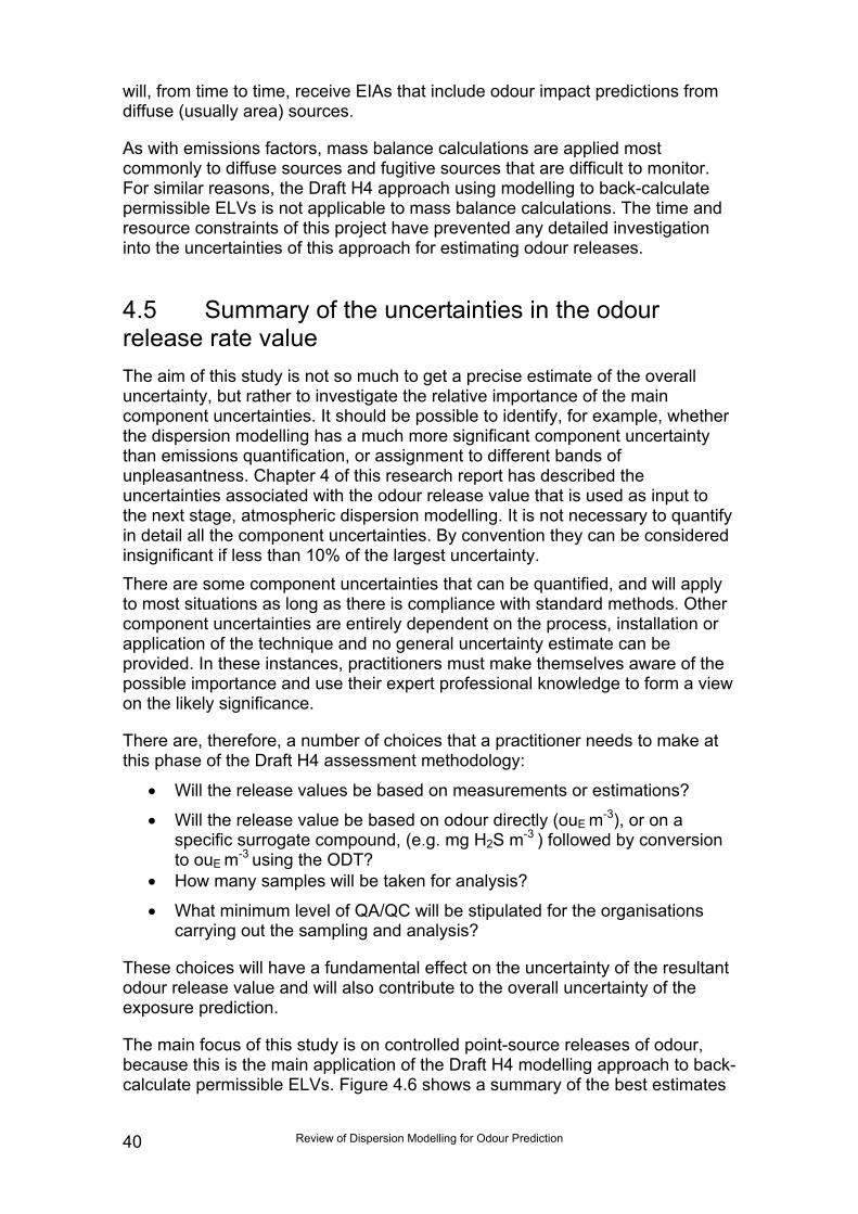
Review of Dispersion Modelling for Odour Prediction40
will, from time to time, receive EIAs that include odour impact predictions fromdiffuse (usually area) sources.
As with emissions factors, mass balance calculations are applied mostcommonly to diffuse sources and fugitive sources that are difficult to monitor.For similar reasons, the Draft H4 approach using modelling to back-calculatepermissible ELVs is not applicable to mass balance calculations. The time andresource constraints of this project have prevented any detailed investigationinto the uncertainties of this approach for estimating odour releases.
4.5 Summary of the uncertainties in the odourrelease rate valueThe aim of this study is not so much to get a precise estimate of the overalluncertainty, but rather to investigate the relative importance of the maincomponent uncertainties. It should be possible to identify, for example, whetherthe dispersion modelling has a much more significant component uncertaintythan emissions quantification, or assignment to different bands ofunpleasantness. Chapter 4 of this research report has described theuncertainties associated with the odour release value that is used as input tothe next stage, atmospheric dispersion modelling. It is not necessary to quantifyin detail all the component uncertainties. By convention they can be consideredinsignificant if less than 10% of the largest uncertainty.There are some component uncertainties that can be quantified, and will applyto most situations as long as there is compliance with standard methods. Othercomponent uncertainties are entirely dependent on the process, installation orapplication of the technique and no general uncertainty estimate can beprovided. In these instances, practitioners must make themselves aware of thepossible importance and use their expert professional knowledge to form a viewon the likely significance.
There are, therefore, a number of choices that a practitioner needs to make atthis phase of the Draft H4 assessment methodology:
• Will the release values be based on measurements or estimations?
• Will the release value be based on odour directly (ouE m-3), or on aspecific surrogate compound, (e.g. mg H2S m-3 ) followed by conversionto ouE m-3 using the ODT?
• How many samples will be taken for analysis?
• What minimum level of QA/QC will be stipulated for the organisationscarrying out the sampling and analysis?
These choices will have a fundamental effect on the uncertainty of the resultantodour release value and will also contribute to the overall uncertainty of theexposure prediction.
The main focus of this study is on controlled point-source releases of odour,because this is the main application of the Draft H4 modelling approach to back-calculate permissible ELVs. Figure 4.6 shows a summary of the best estimates

Review of Dispersion Modelling for Odour Prediction 41
of component uncertainties in the release rate value (obtained bymeasurements) for a controlled point-source.
The Figure show clearly that the use of a specific surrogate compound followedby conversion to ouE m-3 using the ODT adds another layer of uncertainty to thisphase, compared to measuring odour directly as ouE m-3. Simple inspection ofthese component uncertainties suggests that the uncertainty in this conversioncan be the dominant factor affecting the uncertainty of the release value thatgoes into the atmospheric dispersion model. It is recommended that theEnvironment Agency makes clear in its guidance that it prefers odour releaserates to be obtained directly from ouE m-3, and it does not favour the use of aspecific surrogate compound followed by conversion to ouE m-3 using the ODT.
Rev
iew
of D
ispe
rsio
n M
odel
ling
for O
dour
Pre
dict
ion
42Figu
re 4
.6 S
umm
ary
of th
e be
st e
stim
ates
of c
ompo
nent
unc
erta
intie
s in
the
rele
ase
rate
val
ue fo
r a c
ontr
olle
d po
int-
sour
ce
Unc
erta
inty
of o
dour
rele
ase
valu
e
Tem
pora
l unc
erta
intie
s - h
ow w
ell d
oes
the
valu
e re
flect
the
times
cale
of in
tere
st, e
.g. s
hort
term
, ann
ual a
vera
ge?
Situ
atio
n/si
te-s
peci
fic
Spat
ial u
ncer
tain
ties
- doe
s th
e lo
catio
n to
whi
ch th
eva
lue
appl
ies
refle
ct w
hat i
s be
ing
rele
ased
from
the
stac
k?Si
tuat
ion/
site
-spe
cific
Unc
erta
intie
sas
soci
ated
with
mea
sure
men
ts o
fod
our e
mis
sion
s
Unc
erta
intie
sas
soci
ated
with
the
appl
icat
ion
ofth
e te
chni
que
Unc
erta
intie
sas
soci
ated
with
the
tech
niqu
eits
elf
Targ
et m
easu
rem
ent,
ofod
our (
ouE
m-3
)
Mea
sure
men
t, of
vol
ume
flow
(Nm
3 s-1
) ±12
%(p
ositi
on m
eets
M1
stan
dard
)
Sam
plin
g
Ana
lysi
s
Sam
plin
g±2
0%A
naly
sis
-37%
to +
58%
(DD
O to
EN
1372
5)
Thes
e ca
n be
min
imis
ed b
ygo
od Q
A/Q
C
Inpu
t to
disp
ersi
onm
odel
Usi
ng m
easu
rem
ent o
fsp
ecifi
c su
rrog
ate
com
poun
d, e
.g. m
g H
2Sm
-3 )
Mea
sure
men
t of
surr
ogat
eco
mpo
und
±10%
(typ
ical
auto
mat
icte
ch)
How
wel
lsu
rrog
ate
acco
unts
for o
dour
Situ
atio
n/si
te-
spec
ific
Con
vers
ion
to o
u E m
-3
usin
g O
DT
(Sub
ject
to la
rge
erro
rs,
orde
rs o
f mag
nitu
de)
Review of Dispersion Modelling for Odour Prediction 43
5 Phase II – Modelling OdourExposureStep 3 needs to deal with uncertainties which can arise in the way the odoursource strength, and its release characteristics(Section 5.10) , are input to thedispersion model. The odour emission rate needs to be quantified only forinstallations if the risk of ‘causing offence’ is moderate or high. The discussionrelates therefore only to installations for which the risk of causing offence ismoderate or high, such that dispersion modelling is to be undertaken.Dispersion modelling for installations which pose only a low risk of causingoffence would be a disproportionate use of resources. This is discussed furtherin Section 5.3.
Figure 5.1 depicts the various inputs to the dispersion model which contribute tothe overall uncertainty in the model prediction. An attempt at assigning typicalvalues to each component uncertainty is made later in Figure 5.2, on the basisof the discussions presented below in Chapter 5.
5.1 Atmospheric dispersion modelling
The link between the odour emitted at source (Step 3) and the quantity arrivingat a relevant receptor (Step 5) is typically provided by dispersion models (Step4). Environmental models are generally representations of complex systemsabout which there is incomplete knowledge. Quantifying uncertainty is essentialfor the appropriate interpretation of model outputs, particularly when assessingagainst environmental standards.
There is a fundamental difference between the requirements of modelling odourcompared to modelling most other air pollutants. Odours can be perceived overa few seconds, whereas current dispersion models are designed principally tocalculate ‘ensemble mean’ concentrations, typically hourly mean concentrationsas the shortest averaging period for setting short-term air quality standards. Theeffects of odour fluctuations about the ‘ensemble mean’ can be modelledexplicitly (see Section 5.12) or it can be incorporated empirically into statisticalrelationships between ‘ensemble mean’ concentrations (e.g. 98th percentile ofhourly means) and community impacts. There is uncertainty in transposing fromthe hourly – average basis of modelling to the ‘few seconds’ over which actualodour events occur.
A research study has been carried out into uncertainty and model sensitivityanalysis for the ADMS model developed by Cambridge EnvironmentalConsultants Ltd (CERC). The study was not concerned with matters specific toodour prediction (Environment Agency 2002d) but it is recognised that suchanalyses are computationally intensive.
This review is not concerned with the uncertainties associated with screeningtechniques such as the Warren Spring dmax calculation or the H1 screening tool.

Review of Dispersion Modelling for Odour Prediction44
Rather, computerised mathematical atmospheric dispersion models are thefocus of this review.
There is a need to be clear on what units the modelling uncertainty is expressedin. If an odour modelling assessment is being carried out according to the DraftH4 methodology, the exposure at a particular receptor will be predicted as the98th percentile of hourly mean concentrations over a year. This will have units ofouE m-3. Any estimate of uncertainty on this prediction therefore needs to beexpressed in ouE m-3, or as + a percentage of the 98th percentile prediction.
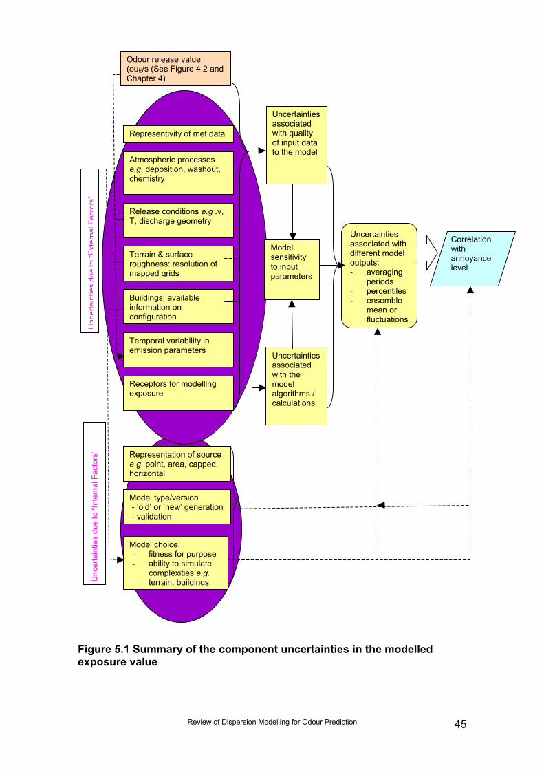
Figure 5.1exposure
Representivity of met data
Atmospheric processese.g. deposition, washout,chemistry
Temporal variability inemission parameters
Terrain & surfaceroughness: resolution ofmapped grids
Buildings: availableinformation onconfiguration
Release conditions e.g .v,T, discharge geometry
Receptors for modellingexposure
Uncertaintiesassociatedwith qualityof input datato the model
Uncertaintiesassociatedwith themodelalgorithms /calculations
Modelsensitivityto inputparameters
Uncertaintiesassociated withdifferent modeloutputs:- averaging
periods- percentiles- ensemble
mean orfluctuations
Correlationwithannoyancelevel
Unc
erta
intie
sdu
eto
“Ext
erna
lFac
tors
”
Representation of sourcee.g. point, area, capped,horizontal
Model type/version - ‘old’ or ’new’ generation - validation
Unc
erta
intie
s du
e to
“Int
erna
l Fac
tors
’
Odour release value(ouE/s (See Figure 4.2 andChapter 4)
Model choice:- fitness for purpose- ability to simulate
complexities e.g.terrain, buildings
Review of Dispersion Modelling for Odour Prediction 45
Summary of the component uncertainties in the modelled value
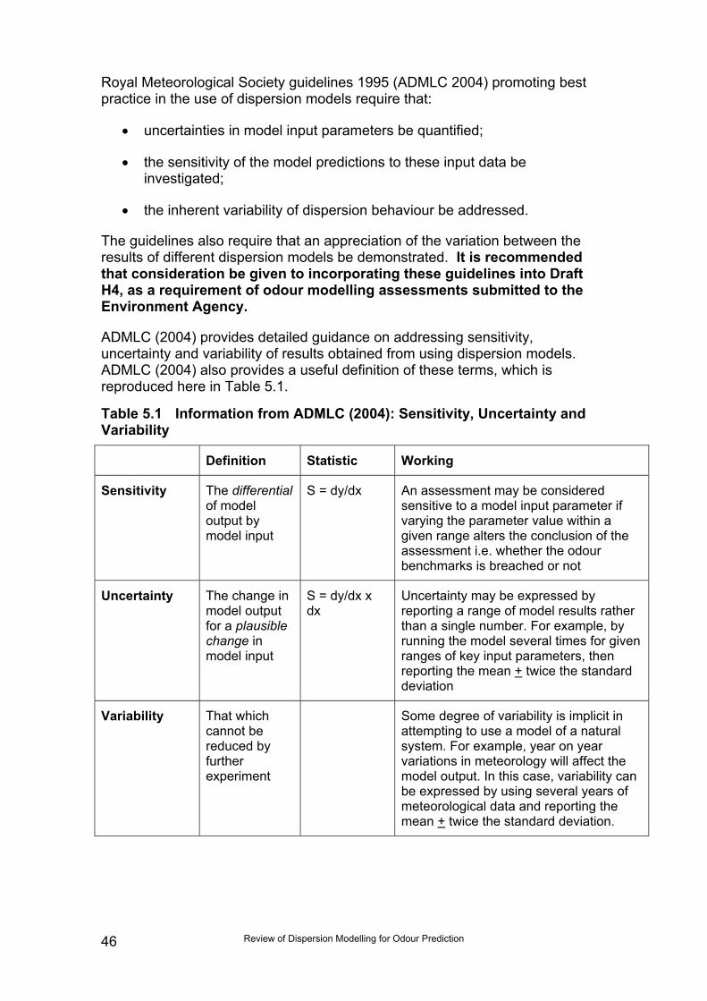
Review of Dispersion Modelling for Odour Prediction46
Royal Meteorological Society guidelines 1995 (ADMLC 2004) promoting bestpractice in the use of dispersion models require that:
• uncertainties in model input parameters be quantified;
• the sensitivity of the model predictions to these input data beinvestigated;
• the inherent variability of dispersion behaviour be addressed.
The guidelines also require that an appreciation of the variation between theresults of different dispersion models be demonstrated. It is recommendedthat consideration be given to incorporating these guidelines into DraftH4, as a requirement of odour modelling assessments submitted to theEnvironment Agency.
ADMLC (2004) provides detailed guidance on addressing sensitivity,uncertainty and variability of results obtained from using dispersion models.ADMLC (2004) also provides a useful definition of these terms, which isreproduced here in Table 5.1.
Table 5.1 Information from ADMLC (2004): Sensitivity, Uncertainty andVariability
Definition Statistic Working
Sensitivity The differentialof modeloutput bymodel input
S = dy/dx An assessment may be consideredsensitive to a model input parameter ifvarying the parameter value within agiven range alters the conclusion of theassessment i.e. whether the odourbenchmarks is breached or not
Uncertainty The change inmodel outputfor a plausiblechange inmodel input
S = dy/dx xdx
Uncertainty may be expressed byreporting a range of model results ratherthan a single number. For example, byrunning the model several times for givenranges of key input parameters, thenreporting the mean + twice the standarddeviation
Variability That whichcannot bereduced byfurtherexperiment
Some degree of variability is implicit inattempting to use a model of a naturalsystem. For example, year on yearvariations in meteorology will affect themodel output. In this case, variability canbe expressed by using several years ofmeteorological data and reporting themean + twice the standard deviation.
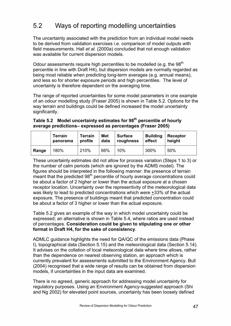
Review of Dispersion Modelling for Odour Prediction 47
5.2 Ways of reporting modelling uncertainties
The uncertainty associated with the prediction from an individual model needsto be derived from validation exercises i.e. comparison of model outputs withfield measurements. Hall et al. (2000a) concluded that not enough validationwas available for current dispersion models.
Odour assessments require high percentiles to be modelled (e.g. the 98th
percentile in line with Draft H4), but dispersion models are normally regarded asbeing most reliable when predicting long-term averages (e.g. annual means),and less so for shorter exposure periods and high percentiles. The level ofuncertainty is therefore dependent on the averaging time.
The range of reported uncertainties for some model parameters in one exampleof an odour modelling study (Fraser 2005) is shown in Table 5.2. Options for theway terrain and buildings could be defined increased the model uncertaintysignificantly.
Table 5.2 Model uncertainty estimates for 98th percentile of hourlyaverage predictions– expressed as percentages (Fraser 2005)
Terrainpanorama
Terrainprofile
Metdata
Surfaceroughness
Buildingeffect
Receptorheight
Range 180% 210% 66% 10% 300% 50%
These uncertainty estimates did not allow for process variation (Steps 1 to 3) orthe number of calm periods (which are ignored by the ADMS model). Thefigures should be interpreted in the following manner: the presence of terrainmeant that the predicted 98th percentile of hourly average concentrations couldbe about a factor of 2 higher or lower than the actual exposure at a chosenreceptor location. Uncertainty over the representivity of the meteorological datawas likely to lead to predicted concentrations which were +33% of the actualexposure. The presence of buildings meant that predicted concentration couldbe about a factor of 3 higher or lower than the actual exposure.
Table 5.2 gives an example of the way in which model uncertainty could beexpressed; an alternative is shown in Table 5.4, where ratios are used insteadof percentages. Consideration could be given to stipulating one or otherformat in Draft H4, for the sake of consistency.
ADMLC guidance highlights the need for QA/QC of the emissions data (PhaseI), topographical data (Section 5.15) and the meteorological data (Section 5.14).It advises on the collation of local meteorological data where time allows, ratherthan the dependence on nearest observing station, an approach which iscurrently prevalent for assessments submitted to the Environment Agency. Bull(2004) recognised that a wide range of results can be obtained from dispersionmodels, if uncertainties in the input data are examined.
There is no agreed, generic approach for addressing model uncertainty forregulatory purposes. Using an Environment Agency-suggested approach (Shiand Ng 2002) for elevated point sources, uncertainty has been loosely defined
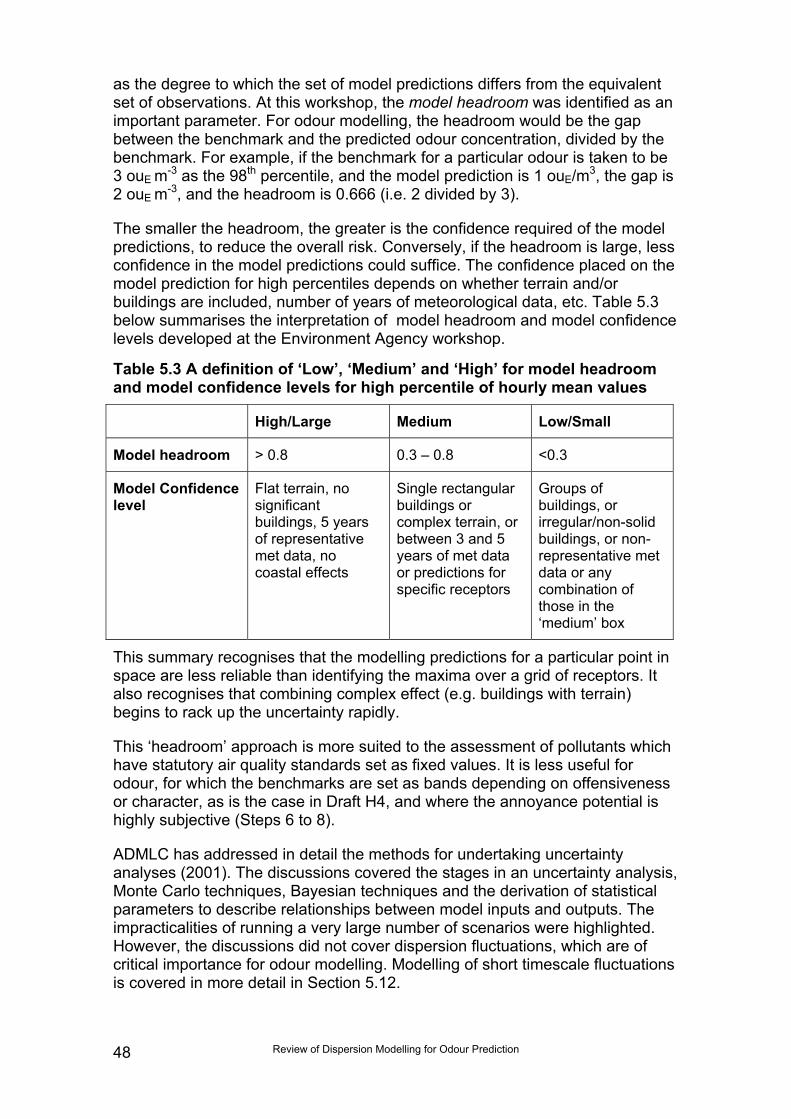
Review of Dispersion Modelling for Odour Prediction48
as the degree to which the set of model predictions differs from the equivalentset of observations. At this workshop, the model headroom was identified as animportant parameter. For odour modelling, the headroom would be the gapbetween the benchmark and the predicted odour concentration, divided by thebenchmark. For example, if the benchmark for a particular odour is taken to be3 ouE m-3 as the 98th percentile, and the model prediction is 1 ouE/m3, the gap is2 ouE m-3, and the headroom is 0.666 (i.e. 2 divided by 3).
The smaller the headroom, the greater is the confidence required of the modelpredictions, to reduce the overall risk. Conversely, if the headroom is large, lessconfidence in the model predictions could suffice. The confidence placed on themodel prediction for high percentiles depends on whether terrain and/orbuildings are included, number of years of meteorological data, etc. Table 5.3below summarises the interpretation of model headroom and model confidencelevels developed at the Environment Agency workshop.
Table 5.3 A definition of ‘Low’, ‘Medium’ and ‘High’ for model headroomand model confidence levels for high percentile of hourly mean values
High/Large Medium Low/Small
Model headroom > 0.8 0.3 – 0.8 <0.3
Model Confidencelevel
Flat terrain, nosignificantbuildings, 5 yearsof representativemet data, nocoastal effects
Single rectangularbuildings orcomplex terrain, orbetween 3 and 5years of met dataor predictions forspecific receptors
Groups ofbuildings, orirregular/non-solidbuildings, or non-representative metdata or anycombination ofthose in the‘medium’ box
This summary recognises that the modelling predictions for a particular point inspace are less reliable than identifying the maxima over a grid of receptors. Italso recognises that combining complex effect (e.g. buildings with terrain)begins to rack up the uncertainty rapidly.
This ‘headroom’ approach is more suited to the assessment of pollutants whichhave statutory air quality standards set as fixed values. It is less useful forodour, for which the benchmarks are set as bands depending on offensivenessor character, as is the case in Draft H4, and where the annoyance potential ishighly subjective (Steps 6 to 8).
ADMLC has addressed in detail the methods for undertaking uncertaintyanalyses (2001). The discussions covered the stages in an uncertainty analysis,Monte Carlo techniques, Bayesian techniques and the derivation of statisticalparameters to describe relationships between model inputs and outputs. Theimpracticalities of running a very large number of scenarios were highlighted.However, the discussions did not cover dispersion fluctuations, which are ofcritical importance for odour modelling. Modelling of short timescale fluctuationsis covered in more detail in Section 5.12.
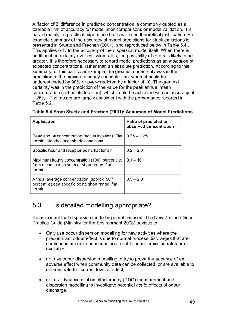
Review of Dispersion Modelling for Odour Prediction 49
A ‘factor of 2’ difference in predicted concentration is commonly quoted as atolerable limit of accuracy for model inter-comparisons or model validation. It isbased mainly on practical experience but has limited theoretical justification. Anexample summary of the accuracy of model predictions for stack emissions ispresented in Stuetz and Frechen (2001), and reproduced below in Table 5.4 .This applies only to the accuracy of the dispersion model itself. When there isadditional uncertainty over emission rates, the possibility of errors is likely to begreater. It is therefore necessary to regard model predictions as an indication ofexpected concentrations, rather than an absolute prediction. According to thissummary for this particular example, the greatest uncertainty was in theprediction of the maximum hourly concentration, where it could beunderestimated by 90% or over-predicted by a factor of 10. The greatestcertainty was in the prediction of the value for the peak annual meanconcentration (but not its location), which could be achieved with an accuracy of+ 25%. The factors are largely consistent with the percentages reported inTable 5.2.
Table 5.4 From Stuetz and Frechen (2001): Accuracy of Model Predictions
Application Ratio of predicted toobserved concentration
Peak annual concentration (not its location). Flatterrain, steady atmospheric conditions
0.75 – 1.25
Specific hour and receptor point, flat terrain 0.2 – 2.0
Maximum hourly concentration (100th percentile)from a continuous source, short range, flatterrain
0.1 – 10
Annual average concentration (approx. 50th
percentile) at a specific point, short range, flatterrain
0.5 – 2.0
5.3 Is detailed modelling appropriate?
It is important that dispersion modelling is not misused. The New Zealand GoodPractice Guide (Ministry for the Environment 2003) advises to:
• Only use odour dispersion modelling for new activities where thepredominant odour effect is due to normal process discharges that arecontinuous or semi-continuous and reliable odour emission rates areavailable;
• not use odour dispersion modelling to try to prove the absence of anadverse effect when community data can be collected, or are available todemonstrate the current level of effect;
• not use dynamic dilution olfactometry (DDO) measurement anddispersion modelling to investigate potential acute effects of odourdischarge.
Review of Dispersion Modelling for Odour Prediction50
This recognises the reliance of the modelling on robust emission data (Phase I).It also recognises the strength of dose-effect data compared to modellingpredictions (Phase III). However, in the UK, dispersion modelling of odours isoften carried out for cases which do not meet these stringent criteria.Consideration should be given to incorporating this guidance into DraftH4.
However, the Environment Agency view may be that if short term emissionsdata and modelling are accurate enough, then it should be possible toinvestigate the potential for short-term events (e.g. failure of abatementequipment) to cause acute impacts. Special care is needed to investigateoccasional acute events, when routine levels of uncertainty will not be adequatefor such cases.
5.4 ‘Old-Generation’ models: COMPLEX1 and LTDF
‘Old-generation’ models have their origins in Gaussian plumes, wherein theconcentration is assumed to be normally distributed in space about the plumecentre-line, and the plume spread is described by the dispersion parameter σxand σy (the root mean square plume widths in the crosswind and verticaldirections, which vary with averaging time). Gaussian plume models have someshort-comings, the most important of which is that they do not represent thestructure of the atmospheric boundary layer in the detail which is possible inmore recently developed similarity-theory based models. New-generationmodels recognise that convection is not a symmetrical process, and this canlead to non-Gaussian concentration profiles, especially in unstable conditions.The ‘old-generation’ models are characterised by their use of ‘Pasquill stabilitycategories’ to describe the state of the atmospheric boundary layer. In contrast,‘new-generation’ models describe atmospheric stability using the Monin–Obukhov length scale (Middleton and Thomson 2002).
It is important to note that both ‘old’ and ‘new’ generation models (and indeedLagrangian and Eulerian models) are essentially statistical in character. Theydo not predict the actual concentration field in a given situation, but rather the‘ensemble mean’ that would be expected if one could repeat the scenario manytimes with essentially identical external conditions. Such repetitions would differby random turbulent fluctuations (Section 5.12).
It has been stated in some of the literature (and colloquially) that the Dutchdose-effect study used the COMPLEX1 dispersion model (Bull, personalcommunication, 2006). However, on investigation, it is concluded that the Dutchdose-effect relationship used LTDF modelling (Darren Hall, Entec, personalcommunication, 2006). It has not been possible to obtain the original Dutchmodelling data; it would have been helpful for the purposes of Project 3 if detailsof the LTDF odour modelling were available for examination. Of particularconcern is the way in which the source strength was defined in the Dutchmodelling.
The Environment Agency’s Report P4-095/TR (2002b) also states that theDutch regulatory model 'Lange Termijn Frequentie Distributie' (LTDF) (VROM1984), was used to calculate exposure for the Dutch dose-effect studies for pig
Review of Dispersion Modelling for Odour Prediction 51
production units (Bongers et al. 2001). This dose-effect relationship has beenadopted by Draft H4 as a tool for predicting annoyance levels in a population.LTDF was the Dutch national regulatory model until 2000, when it was replacedby a new modern Gaussian model. A study re-examining the originalannoyance survey results in 2000 has again cited the dispersion model asbeing the Gaussian LTDF model (Werkgroep Verspreiding Luchtverontreiniging1983).
Although many model inter-comparison studies between 'old' and 'new'generation models have been reported, none have included LTDF. Anymodelling results which the Environment Agency receives as part of an odourassessment in the future will almost certainly be based on ADMS or AERMODPRIME. Although outside the scope of Project 3, it would be useful(perhaps as part of another research project) to attempt to identify anysystematic differences in predictions between LTDF and both of the two‘new-generation’ models, for cases which are relevant to odourassessment e.g. high percentiles, and the relevant range of stack heights.This would identify any bias-type (systemic) differences between the modellingthat established the dose-response relationship, and modelling results whichthe Environment Agency is likely to receive now.
COMPLEX1 was used for the modelling carried out for the planning appealagainst refusal of consent for a wastewater treatment works at Newbiggin-by-the-Sea – the decision of the Inspector (issued in 1993) set a precedent forhourly modelling of the 98th percentile, against a benchmark of 5 ouE m-3 whichwas adopted by the UK odour modelling community and industry for manyyears after the public inquiry.
COMPLEX1 is a module for complex terrain incorporated into the ISCST3model (US EPA 1995). When complex terrain is encountered, the modeldetermines the elevation change for the leading hill and raises the plume heightby half of that amount. This is done in an attempt to allow the plume to respondto the underlying terrain, while maintaining conservatism. It was recognised bythe US EPA that such ISC terrain predictions were very poor, as the modeltended to over-predict significantly, by at least a factor of 2 (USEPA 1999). Thispartly underpinned the development of AERMOD. On this basis, it may beassumed that the use of COMPLEX1 in areas of flat terrain would revert themodelling to the original ISCST algorithms.
5.5 ‘New-Generation’ models: ADMS and AERMOD
‘New-generation’ dispersion models are very versatile in terms of being able toincorporate changes in odour emission rates on anhourly/daily/monthly/seasonal basis. The principal difficulty lies in measuring,estimating or predicting the odour emission rate for the various stages in aproduction cycle/operating regime (Steps 1 and 2). This is particularly importantfor odour assessments where there can often be significant diurnal variation inthe odour source strength.
Review of Dispersion Modelling for Odour Prediction52
Currently, applications for authorisation are most likely to be based onmodelling using ADMS or AERMOD. The relative performance of these modelsis of concern, and has been investigated in detail by Hall et al (2000b) for arange of relatively simple scenarios (though the PRIME algorithms for buildingdownwash effects were not included in AERMOD at the time of that study). Acritical feature of inter-comparisons appears to be the handling ofmeteorological data inputs to the models, especially in the relationshipsbetween Monin-Obukhov length scale inputs.
It is clear that there are significant, case-dependent differences between the two‘new-generation’ models, AERMOD and ADMS. The former was developed bythe US EPA, and the latter was developed by CERC. Hall et al. (2000a)concluded that the greatest differences between the two ‘new-generation’models ADMS and AERMOD is probably in the secondary procedures to dealwith factors such as plume rise, building entrainment and terrain. There is somejustification therefore for assuming that US EPA models (e.g. ISC andAERMOD) should be more akin to each other than the two ‘new-generation’models developed by different organisations. This was been found to be thecase between AERMOD and ISC in relation to the way that they treat buildings.However, AERMOD PRIME has now replaced AERMOD, and has enhancedmethods for treating buildings (Section 5.7).
The Draft H4 Indicative Odour Exposure Standards were derived fromcomparison of the output of an ‘old–generation’ model (LTDF), with annoyancesurveys. Draft H4 states that ‘If using newer models to compare the actualperformance against the benchmark, it is possible that the installation-specificresults may show a numerically higher result than would have been the casewith the use of an older-generation model’. This recognises that an ‘old-generation’ model could give higher predicted ground level concentrations thana ‘new- generation’ models, for the same model input parameters. If so, thenthe Indicative Odour Exposure Standard would need to be lowered if ‘new-generation’ models are being used to predict the impact of the same odour-emitting installation, and assuming everything else remains constant.Conversely, the ‘new-generation’ model would allow the plant a higher odouremission rate to still achieve the same predicted odour concentration (as ouE m-
3) at any particular receptor.
Hall et al (2000a, 2000b) implied that there is less consensus between the ‘new-generation’ models (ADMS and AERMOD) than between the older models (R91and ISC). For Project 3, this assumption could have been useful if it had beenpossible to affirm that LTDF was typical of an ‘old-generation’ model such asISC. However, in the absence of any published inter-comparisons between old-generation models which included LTDF, it is not possible to assume that theresults of LTDF modelling were typical of, or similar to, the results of ISC orR91.
The major effort in model development, besides extending the range ofapplication, has tended towards minimising systematic errors in calculation andin trying to define the degree of uncertainty associated with model calculations.It is common for substantial differences to exist in nominally identicalcalculations between different versions of the same model. Model developerscan argue that the current version of any model is the best validated and best
Review of Dispersion Modelling for Odour Prediction 53
fits the field data. Therefore, there may be little point in now discussing oldermodel variants.
ADMS-4 is expected to be released by CERC in late 2006. The most up-to-daterelease for ADMS at the time of writing (April 2006) is ADMS-3.3. This wasreleased in late July/early August 2005, and replaced ADMS-3.2. At the timethat the Environment Agency let the contract for the project P4-120/2 Ref.13933, the most up-to-date version was ADMS-3.1. Concern has beenexpressed in the past over significant changes in the predictions of differentversions of ADMS.
It is understood that Air Quality Monitoring and Assessment Unit (AQMAU)routinely investigate the performance of different version on their release. It islikely that there are significant differences between ADMS-2, ADMS-3.2 and 3.3in the way building downwash is treated. Moreover, CERC state that ADMS-3.3corrects an error in ADMS-3.2 concerning the calculation of percentiles. ADMS3calculates percentiles by linear interpolation of a probability distribution function(PDF) generated from the predicted hourly concentrations at each receptor.This raises concerns over the calculation of percentiles (notably the 98th
percentile, of relevance to Project 3) in published inter-comparison studies. Italso highlights the more robust approach of identifying the number ofexceedances of an hourly mean benchmark, rather than depending on thesoftware or post-processor to calculate percentiles automatically.
A recent, published inter-comparison of ‘new-generation’ models by AQMAU(Sidle et al. 2004) included ADMS3.1, AERMOD and AERMOD PRIME. Thisstudy concluded that there was greater agreement between the models for the98th percentile than higher percentiles. When buildings were included, it wasobserved that the models showed very different sensitivities to the wind angleand few trends could be discerned. The results of terrain modelling were verysimilar between the US EPA models, but very different to the ADMS3.1 results.The authors concluded that for regulatory purposes, it is advisable tomake use of two models to increase confidence in the model predictions.
5.6 Model inter-comparison studies
Such studies are well-documented, but are in danger of dating very quickly as aresult of newer versions being released to replace older versions. For example,AERMOD PRIME was promulgated recently by the US EPA and this is now thede facto standard for AERMOD. Therefore, it is unlikely that the EnvironmentAgency will any longer receive an application for an odour-emitting processwhich uses AERMOD without the PRIME algorithms, if buildings are present.The Environment Agency is even less likely to receive any applications basedon ISCST3.
Key features of published inter-comparison results are summarised in thisreview where they could be relevant to the types of situation encountered forodour-emitting installations in the UK. For example, studies describing the
Review of Dispersion Modelling for Odour Prediction54
modelling of very tall stacks (greater than 75 m) are excluded *, and the resultsof short averaging period/high percentile (i.e. 98th or greater) calculations onlyare of primary interest. It is unfortunate that no published inter-comparisonstudies have been identified which included LTDF.
Lee et al. (1999) compared the results of AERMOD and ISCST3 for a refinery,predicting the 3-hour high-second high SO2 value (i.e. the second highest, 3-hour mean concentration, which is equivalent to the 99.9th percentile). Thispaper draws attention to an important issue which has relevance for odourmodelling, namely that ISCST3 uses the Pasquill dispersion curves which applyto a ‘sampling time of about 3 minutes’, whereas AERMOD predicts 1-houraverages by design. There were 22 sources on site (stack heights ranging from13 to 41 m), significant downwash effects, and flat terrain. The AERMOD andISCST3 predictions for the 3-hour, high-second high values were within 13% ofeach other, which is surprisingly good agreement for two dispersion models fora high percentile calculation; it may be partly due to the results for the 22sources being aggregated, and the errors cancelling each other out to a largeextent. No systematic trend was observed, one model giving higher resultsthan the other depending on which of four meteorological years was beingmodelled.
Hall et al. (2000a) reviewed inter-comparison studies of ISC, R91, ADMS andAERMOD published prior to September 2000. It is unclear which version ofADMS was used in each of the studies, and this could be a significantconfounding factor. They stated:
‘Only ten studies were found directly comparing either ADMS and AERMODwith each other or with older models….The effects of building entrainment andtopography in particular have been little studied. Little attention has been givento variant versions of model issued over time and any differences betweenthem. A critical feature of inter-comparisons appears to be the handling ofmeteorological data inputs to the models, especially in the relationship betweenMonin-Obukhov length scale based inputs and Pasquill/Gifford stabilitycategories’.
A few relevant, simplified findings of the review carried out by Hall et al. andother inter-comparison studies are reproduced below:
• Hall et al. (2000a) concluded that differences between ‘new’ and ‘old-generation’ models are generally greater in stable and unstable boundarylayers, than in neutral conditions. The 'new-generation’ models tend toproduce more rapid vertical dispersion in unstable flows, and reducedvertical dispersion in stable flows.
• A study by Jones at al. (1995) found that maximum 1-hour meanconcentration (i.e. the 100th percentile) predicted by R91 and ADMS1tended to be different by a factor of between 2 and 3, ADMS-1 generallypredicting the lower concentrations. The stack heights in the Jones et al.
* Previous discussions with Chris Sidle (Environment Agency) concluded that stacks exceeding75 m were very rare for installations of interest to the Agency with respect to odour impact.

Review of Dispersion Modelling for Odour Prediction 55
(1995) study were in the range 10 – 70 m, and three building shapeswere modelled
• Maul et al (1996) compared two versions of R91 with ADMS andISCST2, for stack heights in the range 20 – 200 m – building effects werenot included. Maximum 1-hour mean concentrations (i.e. 100th
percentiles) varied by up to a factor of 4 between models. ADMSproduced significantly more rapid vertical dispersion in convectiveconditions and reduced dispersion in stable conditions. This considerablyaltered the distances at which the maximum ground level concentrationsoccurred.
• Harvey (1998) has presented a comparison of high percentile predictionsfor AERMOD and ADMS, for installations with stack heights of 70 m (witha low building), 50 m (with a low building) and 55 m (no building). Someof these data are summarised in Table 5.5. The 98th percentilepredictions are important for the purposes of identifying any systematicdifferences between ADMS and AERMOD in relation to odourassessment in line with Draft H4.
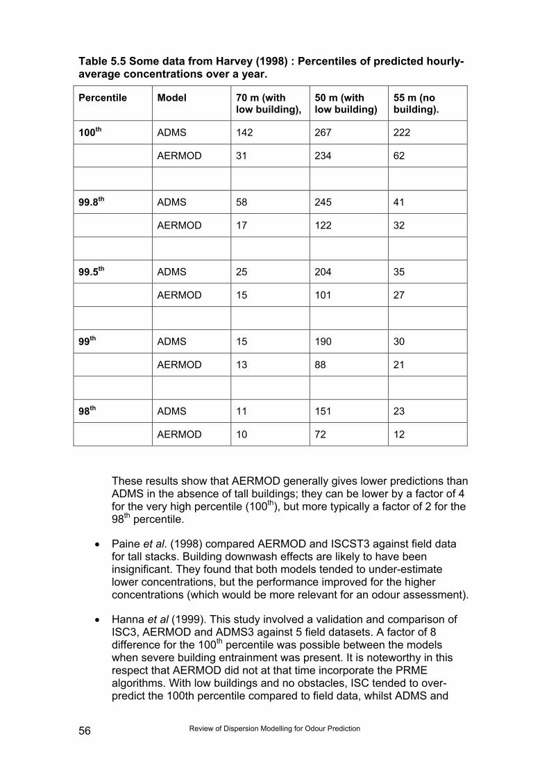
Review of Dispersion Modelling for Odour Prediction56
Table 5.5 Some data from Harvey (1998) : Percentiles of predicted hourly-average concentrations over a year.
Percentile Model 70 m (withlow building),
50 m (withlow building)
55 m (nobuilding).
100th ADMS 142 267 222
AERMOD 31 234 62
99.8th ADMS 58 245 41
AERMOD 17 122 32
99.5th ADMS 25 204 35
AERMOD 15 101 27
99th ADMS 15 190 30
AERMOD 13 88 21
98th ADMS 11 151 23
AERMOD 10 72 12
These results show that AERMOD generally gives lower predictions thanADMS in the absence of tall buildings; they can be lower by a factor of 4for the very high percentile (100th), but more typically a factor of 2 for the98th percentile.
• Paine et al. (1998) compared AERMOD and ISCST3 against field datafor tall stacks. Building downwash effects are likely to have beeninsignificant. They found that both models tended to under-estimatelower concentrations, but the performance improved for the higherconcentrations (which would be more relevant for an odour assessment).
• Hanna et al (1999). This study involved a validation and comparison ofISC3, AERMOD and ADMS3 against 5 field datasets. A factor of 8difference for the 100th percentile was possible between the modelswhen severe building entrainment was present. It is noteworthy in thisrespect that AERMOD did not at that time incorporate the PRMEalgorithms. With low buildings and no obstacles, ISC tended to over-predict the 100th percentile compared to field data, whilst ADMS and
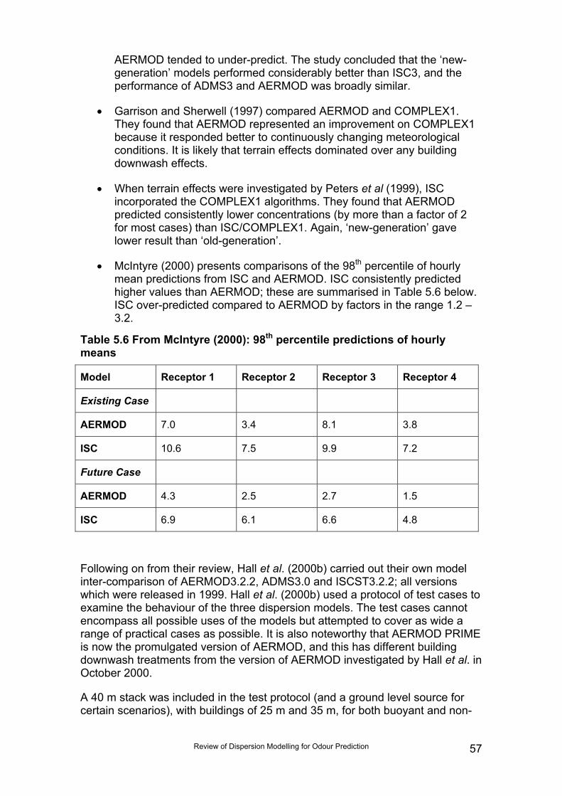
Review of Dispersion Modelling for Odour Prediction 57
AERMOD tended to under-predict. The study concluded that the ‘new-generation’ models performed considerably better than ISC3, and theperformance of ADMS3 and AERMOD was broadly similar.
• Garrison and Sherwell (1997) compared AERMOD and COMPLEX1.They found that AERMOD represented an improvement on COMPLEX1because it responded better to continuously changing meteorologicalconditions. It is likely that terrain effects dominated over any buildingdownwash effects.
• When terrain effects were investigated by Peters et al (1999), ISCincorporated the COMPLEX1 algorithms. They found that AERMODpredicted consistently lower concentrations (by more than a factor of 2for most cases) than ISC/COMPLEX1. Again, ‘new-generation’ gavelower result than ‘old-generation’.
• McIntyre (2000) presents comparisons of the 98th percentile of hourlymean predictions from ISC and AERMOD. ISC consistently predictedhigher values than AERMOD; these are summarised in Table 5.6 below.ISC over-predicted compared to AERMOD by factors in the range 1.2 –3.2.
Table 5.6 From McIntyre (2000): 98th percentile predictions of hourlymeans
Model Receptor 1 Receptor 2 Receptor 3 Receptor 4
Existing Case
AERMOD 7.0 3.4 8.1 3.8
ISC 10.6 7.5 9.9 7.2
Future Case
AERMOD 4.3 2.5 2.7 1.5
ISC 6.9 6.1 6.6 4.8
Following on from their review, Hall et al. (2000b) carried out their own modelinter-comparison of AERMOD3.2.2, ADMS3.0 and ISCST3.2.2; all versionswhich were released in 1999. Hall et al. (2000b) used a protocol of test cases toexamine the behaviour of the three dispersion models. The test cases cannotencompass all possible uses of the models but attempted to cover as wide arange of practical cases as possible. It is also noteworthy that AERMOD PRIMEis now the promulgated version of AERMOD, and this has different buildingdownwash treatments from the version of AERMOD investigated by Hall et al. inOctober 2000.
A 40 m stack was included in the test protocol (and a ground level source forcertain scenarios), with buildings of 25 m and 35 m, for both buoyant and non-
Review of Dispersion Modelling for Odour Prediction58
buoyant releases. The terrain in the vicinity of Porton Down was modelled, withvarious orientations for the source relative to the terrain. Lyneham 1995meteorological data were used. Findings relevant to odour impact assessmentsare reproduced in Table 5.7, which relate to specific 1-hour meteorologicalconditions.
These results show that the ‘new-generation’ models are more likely to givelower predictions for maximum concentrations under user-defined short-termmeteorological conditions (as compared to ISC). However, for unstableconditions, ADMS predicts the highest concentrations. In terms of the distancefrom source to the maximum concentration, AERMOD predicted the peak at fargreater distances under stable conditions compared to the US EPA models.
The results in Tables 5.7 and 5.8 again show that the ‘new-generation’ modelsare more likely to give lower predictions for maximum concentrations underuser-defined short-term meteorological conditions (as compared to ISC). Interms of the distance to the predicted maximum, no systematic differencebetween the models could be identified for the test scenarios.
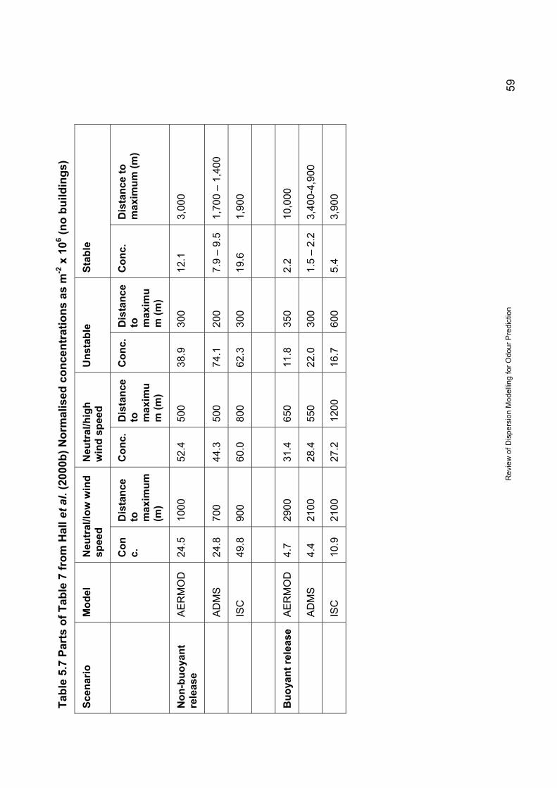
Rev
iew
of D
ispe
rsio
n M
odel
ling
for O
dour
Pre
dict
ion
59
Tabl
e 5.
7 Pa
rts
of T
able
7 fr
om H
all e
t al.
(200
0b) N
orm
alis
ed c
once
ntra
tions
as
m-2
x 1
06 (no
build
ings
)
Scen
ario
Mod
elN
eutr
al/lo
w w
ind
spee
dN
eutr
al/h
igh
win
d sp
eed
Uns
tabl
eSt
able
Con
c.D
ista
nce
to max
imum
(m)
Con
c.D
ista
nce
to max
imu
m (m
)
Con
c.D
ista
nce
to max
imu
m (m
)
Con
c.D
ista
nce
tom
axim
um (m
)
Non
-buo
yant
rele
ase
AE
RM
OD
24.5
1000
52.4
500
38.9
300
12.1
3,00
0
AD
MS
24.8
700
44.3
500
74.1
200
7.9
– 9.
51,
700
– 1,
400
ISC
49.8
900
60.0
800
62.3
300
19.6
1,90
0
Buo
yant
rele
ase
AE
RM
OD
4.7
2900
31.4
650
11.8
350
2.2
10,0
00
AD
MS
4.4
2100
28.4
550
22.0
300
1.5
– 2.
23,
400-
4,90
0
ISC
10.9
2100
27.2
1200
16.7
600
5.4
3,90
0
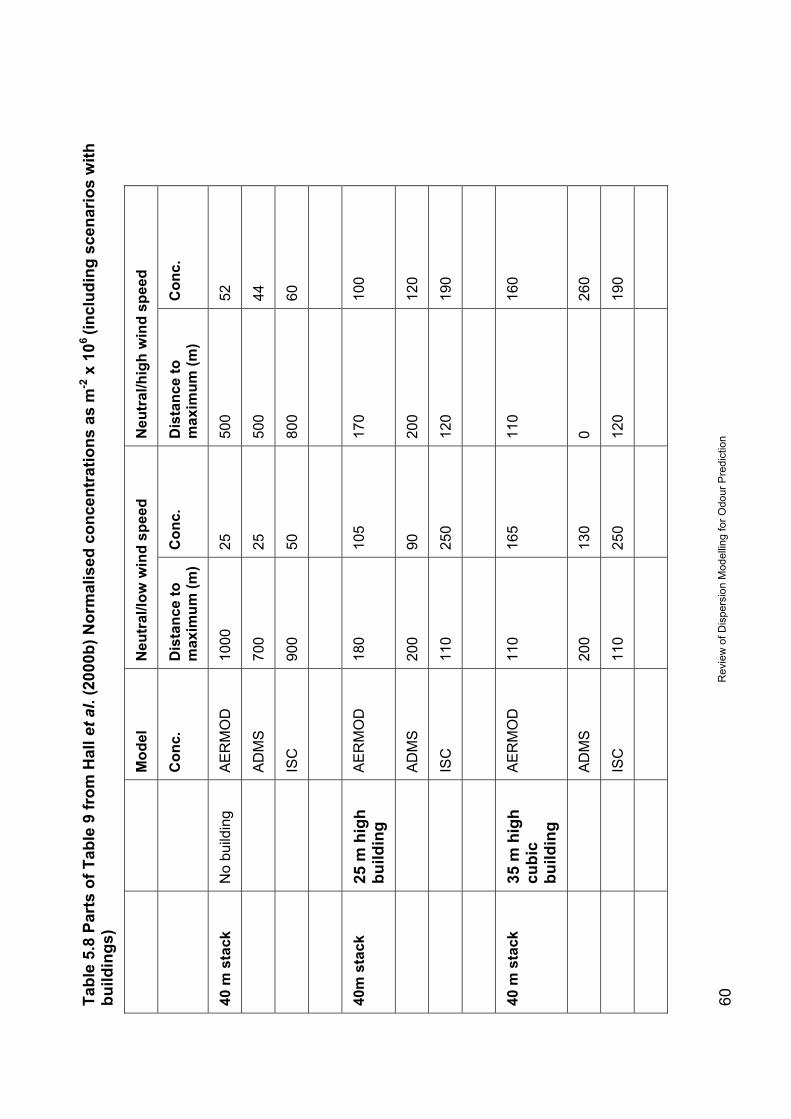
Rev
iew
of D
ispe
rsio
n M
odel
ling
for O
dour
Pre
dict
ion
60Tabl
e 5.
8 Pa
rts
of T
able
9 fr
om H
all e
t al.
(200
0b) N
orm
alis
ed c
once
ntra
tions
as
m-2
x 1
06 (in
clud
ing
scen
ario
s w
ithbu
ildin
gs)
Mod
elN
eutr
al/lo
w w
ind
spee
dN
eutr
al/h
igh
win
d sp
eed
Con
c.D
ista
nce
tom
axim
um (m
)C
onc.
Dis
tanc
e to
max
imum
(m)
Con
c.
40 m
sta
ckN
o bu
ildin
gA
ER
MO
D10
0025
500
52
AD
MS
700
2550
044
ISC
900
5080
060
40m
sta
ck25
m h
igh
build
ing
AE
RM
OD
180
105
170
100
AD
MS
200
9020
012
0
ISC
110
250
120
190
40 m
sta
ck35
m h
igh
cubi
cbu
ildin
g
AE
RM
OD
110
165
110
160
AD
MS
200
130
026
0
ISC
110
250
120
190
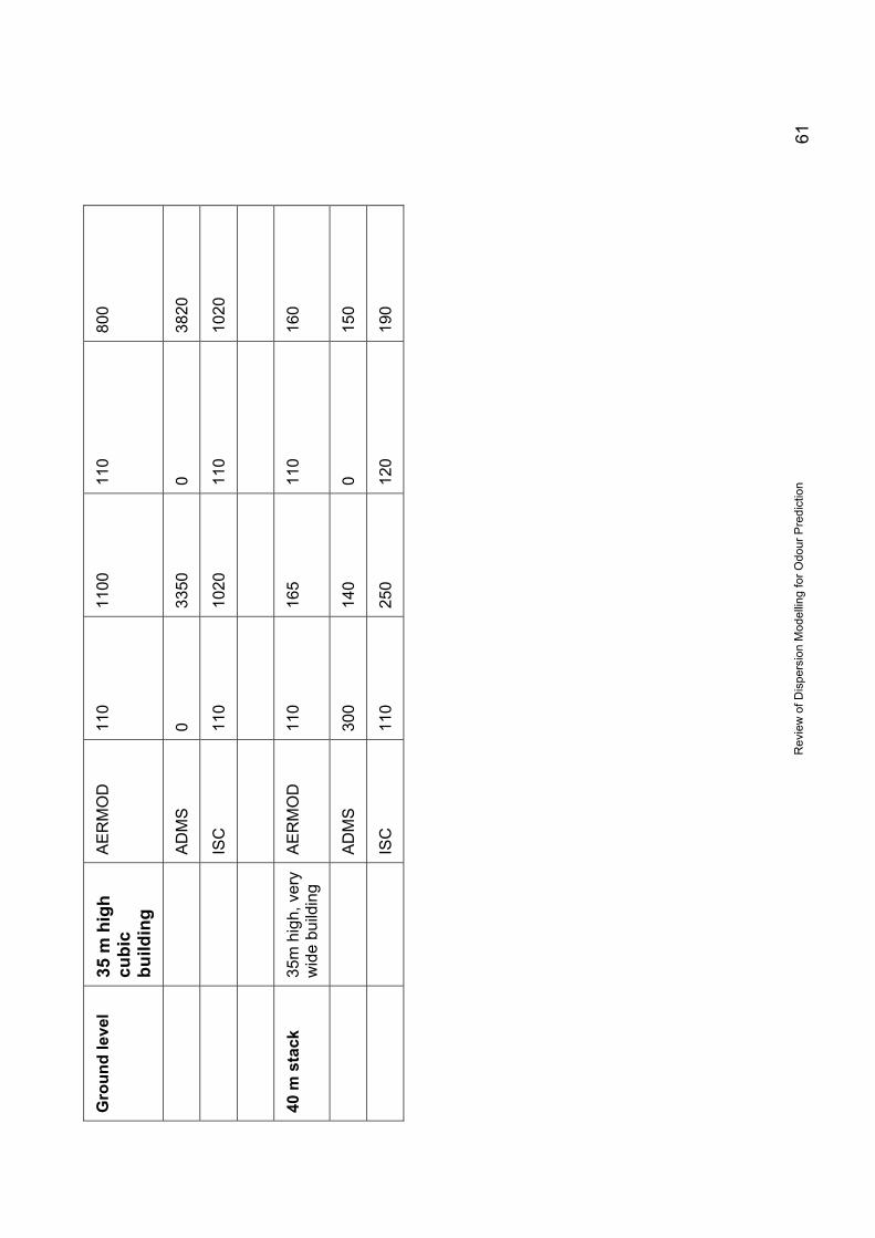
Rev
iew
of D
ispe
rsio
n M
odel
ling
for O
dour
Pre
dict
ion
61
Gro
und
leve
l35
m h
igh
cubi
cbu
ildin
g
AE
RM
OD
110
1100
110
800
AD
MS
033
500
3820
ISC
110
1020
110
1020
40 m
sta
ck35
m h
igh,
ver
yw
ide
build
ing
AE
RM
OD
110
165
110
160
AD
MS
300
140
015
0
ISC
110
250
120
190
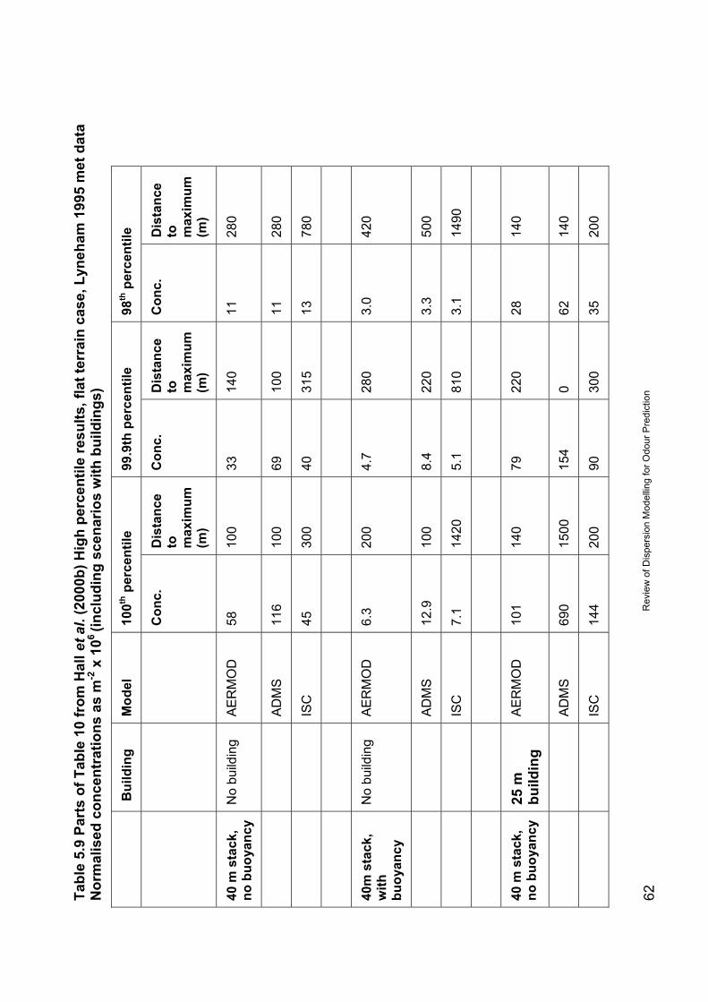
Rev
iew
of D
ispe
rsio
n M
odel
ling
for O
dour
Pre
dict
ion
62Tabl
e 5.
9 Pa
rts
of T
able
10
from
Hal
l et a
l. (2
000b
) Hig
h pe
rcen
tile
resu
lts, f
lat t
erra
in c
ase,
Lyn
eham
199
5 m
et d
ata
Nor
mal
ised
con
cent
ratio
ns a
s m
-2 x
106
(incl
udin
g sc
enar
ios
with
bui
ldin
gs)
Bui
ldin
gM
odel
100th
per
cent
ile99
.9th
per
cent
ile98
th p
erce
ntile
Con
c.D
ista
nce
to max
imum
(m)
Con
c.D
ista
nce
to max
imum
(m)
Con
c.D
ista
nce
to max
imum
(m)
40 m
sta
ck,
no b
uoya
ncy
No
build
ing
AE
RM
OD
5810
033
140
1128
0
AD
MS
116
100
6910
011
280
ISC
4530
040
315
1378
0
40m
sta
ck,
with
buoy
ancy
No
build
ing
AE
RM
OD
6.3
200
4.7
280
3.0
420
AD
MS
12.9
100
8.4
220
3.3
500
ISC
7.1
1420
5.1
810
3.1
1490
40 m
sta
ck,
no b
uoya
ncy
25 m
build
ing
AE
RM
OD
101
140
7922
028
140
AD
MS
690
1500
154
062
140
ISC
144
200
9030
035
200

Rev
iew
of D
ispe
rsio
n M
odel
ling
for O
dour
Pre
dict
ion
63
40 m
sta
ck,
no b
uoya
ncy
35 m
build
ing
AE
RM
OD
174
140
101
140
4414
0
AD
MS
1561
1430
172
140
126
140
ISC
220
200
158
200
4520
0
Review of Dispersion Modelling for Odour Prediction64
5.7 Model inter-comparison results with buildingdownwash effects
Such studies are well-documented but are almost all out-of-date, as morerefined versions of most models are released which claim to have improvedmethods for dealing with downwash effects. Tables 5.8 and 5.9 summarisesome pertinent, historical results. Without buildings, the 98th percentile resultscan be quite similar between ADMS and AERMOD models. However, withbuildings, ADMS and AERMOD predictions can differ greatly, with ADMSpredicting much higher values.
There is concern over a recently disclosed error in percentile calculation withinADMS3.2, which has been reported on release of ADMS 3.3. Moreover, therehave been numerous changes in the building wake/entrainment treatments inADMS with successive versions of the model.
ISC is closer to AERMOD which would be expected for two US EPA modelscontaining similar downwash algorithms. In terms of the distance to thepredicted maximum concentrations, ISC generally gave the peak furthest fromsource, with AERMOD and ADMS predicting more similar distances on mostoccasions.
These published result show that the general order of predictions for highpercentile (98th, 99th and 100th) concentrations in the presence of buildingdownwash effects, is as follows:
• Highest prediction: ADMS
• Lowest predictions: AERMOD
However, this trend is at variance with a more recent study carried out by BV in2004 (for multiple controlled-stack odour emissions at a car-manufacturing plantwith significant buildings), which employed ADMS3.1 and AERMOD (withPRIME algorithms). Stack heights were all 30 m. It was found that AERMODgave higher predictions for the 98th percentile concentration at most receptorlocations, by as much as a factor of 4 at the point of maximum impact, butgenerally about 20% higher than the ADMS3 result at specific locations ofinterest. Receptors were all within 2 km of the emission sources, and somewere within 100 m of certain stack-building configurations.
In this respect, it would have been particularly useful to examine the LTDFmodelling which established the Dutch dose-effect relationship, for the inclusionand treatment of building effects. Regrettably, no information on the technicaldetails of the historical LTDF modelling were available for Project 3.
Just because a model claims to be able to treat buildings and terrain does notmean it works well. ADMLC (2004) highlights the uncertainties surroundingmodels treatment of terrain and buildings, and their sensitivity to surfaceroughness (often overlooked for sensitivity analysis). The entrainment ofplumes in building wakes is of great practical importance and is often the
Review of Dispersion Modelling for Odour Prediction 65
dominant factor controlling acceptable stack heights, especially for low levelstacks. Hall et al (2000b) concluded that AERMOD, ISCST3 and ADMS alltreated near-field building entrainment in quite primitive ways. For example,ADMS approximates the building form into an equivalent rectangular block. Themodel inter-comparison study of Hall et al. concluded that none of the modelswas effective at estimating near-field building plume downwash andentrainment. Subsequent to the work of Hall et al., arguably the most robustfield validation is now available for AERMOD PRIME (Peters et al. 1999).
It has not been possible to demonstrate any relationship between the results ofLTDF and ISC during the course of Project 3. On the basis of the model inter-comparison studies which have been reviewed (Sections 5.6 and 5.7), thefollowing approach could be considered: more than one ’new-generation’model should be used for any odour modelling assessment. The range ofresults obtained from the use of multiple models needs to be inspected, toascertain the risk of breaching the IOES.
5.8 Choice of model
In any modelling study, the choice of model needs to be justified, with particularreference to local building configuration, surface roughness and terrain (Section5.15). There is a need to identify any systematic error (bias), for example onemodel always predicting lower than another.
A variety of dispersion models, different versions of models and approaches tomodelling may be used in applications for authorisation. The applicant mustdemonstrate that the model used is fit for purpose*. Report P4-095/TR(Environment Agency 2002b) acknowledges that:
Ideally, when using dispersion models for odour annoyance prediction,the objective must be to apply the models that were used to establishdose-effect relationships in the underlying epidemiological case studies.
The Dutch regulatory LTDF model was used for the modelling which calculatedthe odour concentration bands for the dose-effect relationship in theNetherlands. LTDF pre-dated the ‘new-generation’ models such as ADMS andAERMOD, but its similarities (if any) to ISC are not known. The results of theLTDF modelling have been largely adopted by Draft H4. Further details of thisGaussian model, and also details of the modelling scenarios, have not becomeavailable for Project 3.
Draft H4 acknowledges that the modelling of odour is still a developing field. Itstates:
‘A range of different models have been used for odour modelling and have anumber of common features, but there are differences in the way that data isdealt with between the older Gaussian model and the ‘new –generation’ modelssuch as AERMOD and ADMS’. * Environment Agency Policy Number Environment AgencyS/2007/1/1
Review of Dispersion Modelling for Odour Prediction66
Fisher (2001) has proposed that when results from several dispersion modelsare available, and assuming that each model has an acceptable level ofperformance (e.g. ADMS and AERMOD), the inevitable inaccuracies in eachmodel should be accepted and both sets of prediction be used to obtain acombined estimate of the impact based on the information available. Forinstallations which present a high risk of odour annoyance, and for whichdispersion modelling is to be carried out, consideration could be given to arequirement in Draft H4 that two appropriate dispersion models be appliedto the investigation. This forms the basis of a risk-based approach.
5.9 Treating predictions from more than one model
Deterministic modelling neglects uncertainty. This has been discussed byFisher (2001) who suggests that the predictions from 2 models could beregarded as either end of a range. He proposes that the prediction of a modelshould not be described as a single number, but as the best estimate of a rangeof numbers, using, for example, fuzzy numbers or fuzzy sets. This uncertaintycan be described in a number of ways. The uncertainty on each number can beused to derive a joint weighting of uncertainty based on statistical methods.
The treatment of uncertainty is inevitably associated with some subjectivejudgements. Fisher concluded that using results from more than one model hasdistinct advantages in decision making, if used with care. Regulatory decisionsshould reflect the underlying uncertainty. These potentially could lead to a betterdescription of imperfect knowledge.
The regulator is best placed to encourage the applicant/operator, on a case-by-case basis, to submit results using more than one dispersion model, and/or tocarry out community dose-effect studies. It would appear that though applicantshave to demonstrate that the assessment is representative and fit for purpose,in practice no mechanism is in place for obliging applicants to submit an odourassessment to this level of detail and complexity.
5.10 Defining model input parametersFor dispersion modelling, data on discharge conditions (effluxvelocity/momentum and heat release) are required, all of which are associatedwith uncertainties due to the measurement or estimation techniques. It may alsobe necessary to measure rate of air flow or ventilation (e.g. number of airchanges per hour). These issues are addressed in Section 4.4.1.3.
5.10.1 Source location
It is not unreasonable to expect that, for the vast majority of installations, thelocations of the odour source/s (stack or areas of known shape) should beknown with very high precision e.g. an OS grid co-ordinate to the nearest 1 m.However, the predictions of dispersion models, if used to identify the point of
Review of Dispersion Modelling for Odour Prediction 67
maximum odour impact, can have uncertainties of hundreds of metres. It isimportant to define the stack location to the nearest metre because then therelative locations/proximity of nearby buildings can be treated appropriately bybuilding downwash algorithms. Area sources need to be sized and locatedaccurately so that the total odour emitted (gs-1) is calculated correctly. Withmodern GIS interfaces to dispersion models, accurate positioning of source,buildings, terrain heights, site boundaries and receptors renders negligible theuncertainties in dispersion modelling results arising from mis-positioning ofthese elements. The uncertainties in dispersion modelling exercises whichinclude buildings and terrain are discussed in Sections 5.7 and 5.15respectively.
5.10.2 Horizontal releases
Dispersion models were formulated for unobstructed vertical releases i.e.chimneys. The dispersion of pollutants from horizontal pipes lends itself more tocomputational fluid dynamics (CFD) modelling, and cannot readily beinvestigated using practical, proprietary models. Guidance from the US EPAstates that an exit velocity of 0.001 ms-1 should be assumed for a horizontalrelease, in order to eliminate the momentum plume rise (J. Hill, TrinityConsultants, personal communication, January 2006). In addition, stack tipdownwash in the model must be switched off, whether or not there are buildingspresent. Stack tip downwash calculations are inappropriate for horizontalstacks. The details of the modelling approach adopted by the applicant formodelling horizontal releases should be checked for these assumptions. It mustbe recognised that the uncertainty on a 98th percentile prediction for horizontalreleases will be very high, but that the prediction is likely to be an overestimate.Therefore, it is recommended that careful consideration be given to thevalidity of odour dispersion modelling for horizontal releases.
5.10.3 Capped release points
Dispersion models were formulated for unobstructed vertical releases, i.e.chimneys. Guidance from the US EPA states that an exit velocity of 0.001 ms-1
should be assumed for a stack with a cap, in order to minimise the momentumplume rise (J. Hill, Trinity Consultants, personal communication, January 2006).In addition, stack tip downwash should be maximised because the cap willprobably generate such downwash most of the time. The resulting predictions ofdownwind concentrations may err slightly on the high side. The details of themodelling approach adopted by the applicant for modelling stacks with capsshould be checked for these assumptions. It must be recognised that theuncertainty on a 98th percentile prediction for capped releases will be very high,but that the prediction is likely to be an overestimate. Therefore, if such a caseis modelled, a risk-based approach is needed: if the predicted odourconcentration is low, then even with modelling uncertainty there might not be aproblem.
Review of Dispersion Modelling for Odour Prediction68
5.10.4 Multiple sources
The results of dispersion models are inherently more uncertain in the followingorder:
• Single stack;
• Multiple stacks spaced well apart;
• Multiple stacks in close proximity;
• Single area source;
• Multiple area sources.
• Non-vertical or obstructed releases.
On this basis, if multiple area sources, non-vertical or obstructed releases aremodelled, it must be recognised that there could be large uncertainties in modelpredictions. A risk-based approach is needed. If the predicted odourconcentration is low, then even with model uncertainty there might not be aproblem.
This ranking does not take account of how odours from different ‘plumes’ mayreact with each other, change their characters on mixing, etc. It is not possiblewith current dispersion models to account for these factors, though most ‘new-generation’ models (e.g. ADMS3, AERMOD PRIME) are very capable of sourceapportionment for conservative pollutants. They can screen out certain sourcesin relation to particular receptors, enabling a detailed investigation ofuncertainties associated with only the significant sources. However, it isimportant to bear in mind that odours are not simply additive, like otherconservative pollutants. Masking and synergistic effects are complex and varyfor each mixture of odorant. This is discussed in detail in the Literature Reviewfor Project 2.
Where there are multiple sources of odour and/or mixtures of chemicalcompounds, dispersion modelling is likely to over-predict downwind odourimpacts. This is because the diluted odour mixture will be dominated by themore offensive components in the mixture, which mask the less offensivecomponents. This over-prediction could be a significant uncertainty in theoverall odour impact assessment. The New Zealand Technical Report (Ministryfor the Environment 2002) considers two options to moderate the effect of thisover-prediction:
• Where the odour discharges on a site can be classified according to theiroffensiveness (e.g. ‘very offensive’ and ‘slightly annoying’), the ‘veryoffensive’ sources are likely to dominate the ‘slightly annoying’ sources(unless the latter has a very high predicted downwind concentrationrelative to the other group). Therefore, the groups of sources can bemodelled separately.
Review of Dispersion Modelling for Odour Prediction 69
• Where a small number of sources on a site are of much loweroffensiveness than the others, then the odour emission rate determinedfor these least offensive odour sources could be corrected downwards bydividing the source’s emission rate by suitable factors.
Consideration could be given to the incorporation of these options intofuture revisions of Draft H4, in order to reduce the uncertainty associatedwith modelling multiple odours on a single site. The guidance in Draft H4currently is as follows:
• Where sources are spread across a large installation, it may beappropriate to consider individual or groups of sources in terms of thespecific receptors that may be affected. There may also be a need toconsider the effect of distance from the source to different receptors,depending on wind direction.
• Where sources are completely different in terms of their odourcharacteristics, it may be better to consider them separately in terms ofimpact on receptors.
5.10.5 Area and near-ground sources
Published/documented validation of dispersion models against fieldmeasurements for real area sources is scarce. Dispersion models weredeveloped primary for single chimneys, but have been modified subsequently totreat other types and numbers of source. In this respect, it would have beenparticularly interesting to examine the LTDF modelling (which established theDutch dose-effect relationship) for the inclusion of area and/or multiple sources.
It is not clear whether ADMS3.3 has been validated against field measurementsfor single area or volume industrial sources. CERC refer to the OPTEX andDuke Forest experiment, but these scenarios had multiple sources, includingpoint sources, and the area/volume sources may not have been dominant(Personal communication with Catheryn Price, CERC, 1 February 2006). CERCalso refer to validation of the line and volume sources in ADMS-Urban andADMS-Roads, but these tests were exclusively for road traffic emissions, notindustrial releases. This raises concerns about the applicability of area andvolume source algorithms in ADMS3 for industrial odour releases.
AERMOD and ADMS treat area sources in different ways: AERMOD assumes avirtual upstream point source, whilst ADMS describes dispersion from elementswithin the source. Significant differences in results are to be expected. Fieldvalidation for area sources in isolation have not been found.
Previous discussions with Chris Sidle (Environment Agency) concluded thatstacks exceeding 75 m were very rare for installations of interest to theEnvironment Agency with respect of odour impact **. Area sources of odour arepredominantly less than 5 m in height.
** Modelling scenario scoping previously carried out for earlier specification for Project 3.
Review of Dispersion Modelling for Odour Prediction70
Some ‘new-generation’ dispersion models cannot include building downwasheffects at all for area sources. If buildings are present near area sources andrelevant receptors are also within close range, there may be no wisdom inattempting modelling at all if the models are being used to the extremes of theircapabilities in such scenarios.
Therefore, the following building and source configurations are ranked in orderof decreasing certainty with respect to dispersion modelling predictions:
• Elevated stack with no nearby buildings;
• Low stacks/near ground level point sources with no buildings;
• Elevated stacks with buildings;
• Low stacks/near ground level point sources with buildings/ Ground levelarea sources with no buildings;
• Ground level or low area sources in the presence of buildings.On this basis, it must be recognised that the modelling of low stacks orarea sources, where nearby buildings are present, is subject to largeuncertainties. A risk-based approach is needed: if the predicted odourconcentration is low, then even with model uncertainty there might not be aproblem.Establishing such a hierarchy for treating model uncertainty is not a newconcept. R. Timmis (Personal communication in Fisher 2001) has proposed ahierarchy for treating model uncertainty in dispersion calculations. Instraightforward cases of a flat terrain and no buildings, one could assume thatmodels are accurate within a factor of 2 (or some other value accepted by themodelling community). For the more complex cases, additional factors ofuncertainty arise (perhaps further factors of 2) to account for the additionaluncertainty (in the ways models account for buildings, for example). There is aconcern that this could soon lead to very large factors of uncertainty as onemultiples the factors together; in practice however, additional complexity usuallyjust involves a single extra process. Sometimes complexity is not necessarilymultiplicative and bounds on possible ranges arise.
If after allowing for this hierarchy of uncertainty, the range of results from twodifferent models still do not overlap, the difference between the models isdeemed to be significant. The reasons for a significant difference are varied.The models may be using different algorithms, e.g. plume behaviour near thetop of the boundary layer, or near the top of a hill.
Fisher (2001) recognised that the treatment of uncertainty is inevitablyassociated with some subjective judgements. Using results from more than onemodel has distinct advantages in decision making, if used with care.
Review of Dispersion Modelling for Odour Prediction 71
5.11 Peak-to-mean ratios
It is important to note that the Draft H4 Indicative Odour Exposure Standards donot include any dependence on peak-to-mean ratios. The EnvironmentAgency’s view is that statistical relationships between modelled percentiles ofhourly average concentrations and surveys of the level of annoyance currentlyprovide a more robust method of determining odour exposure (Phase III).Fluctuations are the differences between a specific dispersion occurrence (or“realisation”) and the ensemble mean of all such occurrences as given by adispersion model. The relationship between the ensemble mean and fluctuatingplume concentrations has been described in many papers (Hall and Kukadia1994, CERC 1998). Conventional dispersion models struggle to treat short-termvariability; this is discussed by Best et al. (2004), where various methods foraccounting for fluctuations in a crude way (e.g. peak-to-mean ratios) aresummarised.Peak-to-mean ratios do not account for the fundamental differences betweenthe distribution of the mean and fluctuating components of concentration in aplume. An important feature of the distribution of concentration with time at aparticular point in a dispersion plume is that if does not have a nominaloccasionally recurring ‘peak’ value, only the probability that some particularvalue will occur.
While more work is required into the relationship between odour nuisance andthe detection of odour over short time-scales, it has been proposed that it isunlikely that a highly intermittent detectable odour with a mean concentrationwell below the detection threshold would cause a nuisance (Simms et al. 1999).Consequently, the effects of very short-term fluctuations (over a matter ofseconds) can probably be adequately modelled by considering an averagingperiod of 3 minutes or similar. Some regulatory authorities (e.g. in Australia)have set odour thresholds based on a 3-minute averaging period for modelling.
Draft H4 recognises that there are a number of areas in odour modelling whichneed further validation, such as peak-to-mean ratios (Appendix 4 Part 1) andappropriate averaging times. It has been shown that there are potentially largedifferences between area near-ground level sources and tall point sources interms of the downwind fluctuation to which a receptor would be exposed.Elevated point sources can produce considerably greater peak-to-mean ratiosthan area sources.
There is other evidence that the frequency and magnitude of peaks in odourconcentration over timescales of seconds and minutes are determining factorsfor the perception of odour (Phase III). At low concentrations, a rapidlyfluctuating odour is often more noticeable than a steady background. Smallscale meteorological variations mean that the peak values can be some tentimes higher than the 1-hour mean values for point sources within the samegeneral weather situation.
The Draft H4 guidance is at variance with the guidance in New Zealand(Ministry for the Environment 2002) which advises that an ‘annoyancethreshold’ (typically 5 ouEm-3 for the mean concentration) is divided by a peak-
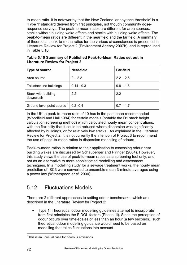
Review of Dispersion Modelling for Odour Prediction72
to-mean ratio. It is noteworthy that the New Zealand ‘annoyance threshold’ is a‘Type 1’ standard derived from first principles, not though community dose-response surveys. The peak-to-mean ratios are different for area sources,stacks without building wake effects and stacks with building wake effects. Thepeak-to-mean ratios are different in the near field and the far field. A summaryof theoretical peak-to-mean ratios for the various circumstances is presented inLiterature Review for Project 2 (Environment Agency 2007b), and is reproducedin Table 5.10.
Table 5.10 Summary of Published Peak-to-Mean Ratios set out inLiterature Review for Project 2
Type of source Near-field Far-field
Area source 2 – 2.2 2.2 – 2.6
Tall stack, no buildings 0.14 - 0.3 0.8 – 1.6
Stack with buildingdownwash
2.2 2.2
Ground level point source * 0.2 -0.4 0.7 – 1.7
In the UK, a peak-to-mean ratio of 10 has in the past been recommended(Woodfield and Hall 1994) for certain models (notably the D1 stack heightcalculation screening method) which calculated hourly mean concentrations,with the flexibility that it could be reduced where dispersion was significantlyaffected by buildings, or for relatively low stacks. As explained in the LiteratureReview for Project 2, it is not currently the intention of Project 3 to recommendthe use of peak-to-mean ratios in dispersion modelling of odours.
Peak-to-mean ratios in relation to their application to assessing odour nearbuilding wakes are discussed by Schauberger and Piringer (2004). However,this study views the use of peak-to-mean ratios as a screening tool only, andnot as an alternative to more sophisticated modelling and assessmenttechniques. In a modelling study for a sewage treatment works, the hourly meanprediction of ISC3 were converted to ensemble mean 3-minute averages usinga power law (Witherspoon et al. 2000).
5.12 Fluctuations Models
There are 2 different approaches to setting odour benchmarks, which aredescribed in the Literature Review for Project 2:
• Type 1: Theoretical odour modelling guidelines attempt to incorporatefrom first principles the FIDOL factors (Phase III). Since the perception ofodour occurs over time-scales of less than an hour (a few seconds), suchtheoretical odour modelling guidance would need to be based onmodelling that takes fluctuations into account.
* This is an unusual case for odorous emissions
Review of Dispersion Modelling for Odour Prediction 73
• Type 2: Empirical odour modelling standards are derived from theempirical relationship between odour exposure and annoyance whichhas actually been measured by a community survey. The IndicativeOdour Exposure Standards in Draft H4 are derived from this method.The fluctuations in odour concentrations are accounted for in thecommunity response in this case, rather than up-front in the dispersionmodelling or exposure predictions.
A number of numerical models have been developed for predicting thefluctuation concentrations in dispersing plumes. Fluctuation models attempt tocalculate specific occurrences (or “realisations”) of concentrations around theensemble mean value. Most of these models predict the bulk statisticalproperties of the plume, so are of more limited assistance in dealing withquestions of intermittency and the frequency of repetition of fluctuating peaks.Neglecting the effect of turbulent fluctuations in modelling can lead to theunderestimation of these peak values and hence of the overall short-termimpact of a release.It is important to note that in contrast with ensemble mean odourconcentrations, the frequencies of high concentration events due to fluctuationsdo not scale up or down proportional to the odour emission rate. Thus a halvingof emissions will not halve the frequency of high concentration events above agiven concentration value due to fluctuations.Conventional models predict the average concentration over a period of an houror more. Normal atmospheric turbulence is sufficient to cause local windvelocity to vary rapidly in both speed and direction and thereby to cause rapidfluctuations in the concentrations of an airborne pollutant at a fixed receptorposition. It is difficult to predict the short-term peak concentrations with anyconfidence, but it is possible to derive a probability distribution function (PDF) ofconcentration and to determine what fraction of this PDF exceeds thebenchmark or threshold (Lee and Stewart 1999). This approach is attempted bymodels such as Omonos * and the fluctuations facility in ADMS3 (Dyster et al.1999).
Omonos can model single and multiple, point and area sources. Like ADMS3,this model predicts the likelihood of the concentration exceeding the thresholdvalue. Omonos makes use of the meandering plume model approach. Omonosuses the Pasquill-Gifford curves (or their mathematical equivalents) to generatethe hourly mean concentrations; it takes this output then calculates fluctuationintensities and intermittency (J.R. Stewart, Queen’s University of Belfast,personal communication, January/February 2006).
When modelling multiple point sources, the total 1-hour mean concentration atany receptor is additive. However, probabilities of exceeding the odourbenchmark cannot be obtained by summing the concentration from individualsources. Furthermore, addition does not address the situation whereinstantaneous concentrations for each point source lie below the thresholdconcentrations but their sum exceeds the threshold level. Omonos includes anumerical method for combining probabilities from multiple point sources which
* Developed by QUESTOR at Queens University of Belfast
Review of Dispersion Modelling for Odour Prediction74
incorporates the concentration fluctuation behaviour of each individual plume. Amodified method allows for the prediction of probability of exceeding thebenchmark from an area source.
The basis of odour assessment in Germany is the ‘odour hour’ (Janicke et al.2004). By definition, an hour is an ‘odour hour’ if, within this hour, odour isperceived for at least 10% of the time. Odour assessment is then based on thefrequency of occurrence of ‘odour hours’ within a year.
Concentration fluctuation models are also being tested in other countries forodour regulation (Lofstrom 2004). The Lagrangian dispersion modelAUSTAL2000G has been developed for calculating the frequency of theseconcentration fluctuations over an hour. The odour dispersion model of theFinnish Meteorological Institute (ODO-FMI) has the ability to represent theshort-term peak values of odour concentration. It uses the meandering plumemethod for point sources and probability density function modelling for area andvolume sources (Pietarila and Savunen 2004).
Comparison of ‘odour hour’ modelling results against odour frequencymeasurements have been presented for a piggery (Janicke et al. 2004), usingthe German regulatory AUSTAL2000G Lagrangian dispersion model. The fieldvalidation exercise released a passive tracer (SF6) simultaneously with theodorous emission, to measure the ensemble mean hourly concentrations, inorder to relate the fluctuating concentration to the ensemble mean, and derive a‘perception function’. The same scenario was also investigated using windtunnel modelling. Consideration should be given to carrying out investigations ofthis nature in UK-specific situations, with the commonly used ‘new-generation’models.
There is a difficulty in that detailed modelling (e.g. using fluctuations) is likely tobe inappropriate for many odour sources due to the wide potential variation inodour emission rates and hence difficulty in obtaining accurate source inputdata. It would be inappropriate to aim for ever-increasing sophistication inmodelling outputs when the reliability and confidence in the input data(particularly that pertaining to the odour emission rates, Phase I) is low.Moreover, buildings cannot be accounted for in ADMS3 when modellingfluctuations. Concentration fluctuations will be significantly modified whenmaterial becomes incorporated within a building wake region. The developers ofADMS (CERC, Simms et al. 1999) state that the additional mixing involved willtend to reduce the peak concentrations, giving a more uniform, less intermittentstructure to the concentrations. Entrainment in the turbulent mixing cavitybehind a building is particularly common at wastewater treatment works, andhas been the subject of discussion.Also, there are few supporting social surveys for the dose predicted usingfluctuation modelling. On the other hand, it may be argued that the response toodour in the social/annoyance surveys includes the effect of concentrationfluctuations. A person’s perception will inevitably incorporate his/her experienceof fluctuations rather than any experience of ensemble means. This is becauseensemble means are a form of statistical summary and so do not generallyoccur in any particular time and place in the field.
Review of Dispersion Modelling for Odour Prediction 75
Validation of any models against predictions of odour concentration is almostimpossible, because it is not possible to measure ambient odour concentrationsin real time using DDO. Limited attempts have been made to measurefluctuations in concentrations using SO2 or other tracers over time-scales ofless than an hour.
5.13 High percentiles
For the 98th percentile prediction, the model requires an entire year of hourlyemission rates. Appendix 4 of Draft H4 Part 1 states that when the odouremission rate and/or other model input parameters fluctuate, then anassessment of this variation should be undertaken.
Although the Draft H4 Indicative Odour Exposure Standards are set as the 98thpercentile of hourly means, many studies have highlighted the significance ofthe 100th, 99.9th and 99th percentiles. The perception and annoyanceassociated with an odour (of particular character) may in fact be related to thesepercentiles, as well as the 98th percentile. The relationship between these highpercentiles and the 98th percentile needs to be investigated. The relationshipdepends on stack height and model choice, and needs to be investigatedfurther in dose-effect studies in the UK. The level of annoyance in thecommunity may be dictated by the percentiles higher than the 98th percentile; itmay be that complaints are actually driven by the top 0.5 % of hourly meanconcentration. This is discussed in the Literature Review for Project 2.
The uncertainty of a model increases for higher percentiles (Tables 5.5 and5.9). Report P4-095/TR (Environment Agency 2002b) states that in the UK, the99th percentile is roughly twice the 98th percentile, but the source of this findingis not transparent.
Quoting model outputs as percentiles implies a far greater confidence in modelpredictions than is reasonable. It may be more useful to report the number ofoccurrences/prediction of hourly concentration above a benchmark in any yearof meteorological data.
Different values of percentile compliance are in use around the world. Miedema(1992) indicated that higher percentile concentrations were best correlated toodour annoyance when the emission source was active for less than 50% of thetime. Therefore, for highly variable and intermittent sources, the 99.9th
percentile concentration may be a stronger determinant of odour annoyancethan the 99.5th percentile.
The Literature Review for Project 2 (Environment Agency 2007b) suggests thatthere is little convincing evidence to support the use of any particular percentilecomponent. The percentage exceedance calculated by the model does notnecessarily mean that odour nuisance will occur for all those hours, andreasons are set out in the Review.German field work (Both and Koch 2004) suggests that frequency is theoverwhelming factor in determining annoyance, more important than odourintensity; how often you are annoyed is more important for complaints than how
Review of Dispersion Modelling for Odour Prediction76
acutely you are annoyed at the time when annoyance occurs. This is becausefrequent annoyance is more likely to detract from people’s quality of life/amenitythan occasional acute annoyance.However, most odour modelling guidelines take both frequency and intensity(usually via concentration) into account, for example an hourly odourconcentration below the relevant Draft H4 Indicative Odour Exposure Standard,to be predicted for at least 98% of the hours in the year.
A recent, published inter-comparison of ‘new-generation’ models by AQMAU(Sidle et al. 2004) included ADMS3.1, AERMOD and AERMOD PRIME. Thisstudy concluded that there was greater agreement between the models for the98th percentile than higher percentiles. For this reason, and in the absence ofany UK specific dose-response studies investigating higher percentiles forannoyance correlation, it is recommended that, for the present, Draft H4maintains the 98th percentile as the parameter for odour concentrationprediction.
Dutch case studies reported by Miedema (1992) indicated that higher percentileconcentrations were best correlated to odour annoyance when the emissionsource is active for less than 50% of the time. Therefore, for highly variable andintermittent sources, the 99.9th percentile concentration may be a strongerdeterminant of odour annoyance than the 99.5th. Dose-response studies inEngland and Wales are awaited before Draft H4 can consider the use of otherpercentiles for odour assessment.
A new assessment parameter has been proposed in Denmark that recognisesthat short and tall stacks complying with the same maximum concentration limitas a percentile will probably result in different odour exposure. This is becausethe critical meteorological parameters occur more often for low stacks than fortall stacks. It has been proposed that a single unifying assessment parameter isused that accumulates all odour concentrations above the odour thresholds andweights the frequency of the individual odour concentrations with the intensity(which is proportional to the log concentration).
5.14 Meteorology
Dispersion behaviour depends critically on the state of the atmosphere.However, the availability of meteorological data is limited. The atmosphere issubject to natural variability, within a given, defined state or on a statistical basisfrom one year to the next (Hall et al. 1999). The way in which meteorologicaldata is pre-processed prior to the model carrying out the dispersion calculationscan have a significant effect on the predictions of the model.
It is likely that differences between models reflect the uncertainties in estimatingturbulent dispersion in the atmospheric boundary layer. Low wind speed andvery stable conditions are difficult to represent in any dispersion model, and inthese situations, the predicted peak ground level concentrations can varywidely. The difficulties which commonly-use models have with dealing with lowwind speed/stable conditions are well documented, and therefore theuncertainty can be taken into account, albeit qualitatively. It follows that this can
Review of Dispersion Modelling for Odour Prediction 77
give rise to predictions of high percentile concentrations that also vary widelybetween models.
Draft H4 recognises that the meteorological data obtained from a Met. Officeobserving station and used for dispersion modelling may not always reflect verylocalised conditions for example a valley location producing its own inversions.These conditions would not be picked up even by 5 or more years ofmeteorological data from a remote observing station; Environment Agencyguidelines on modelling for PPC purposes stipulates the use of 5 years ofmeteorological data. Where unusual weather conditions are suspected asbeing the cause of odour occurrences, it may be appropriate to model specifichours of theoretical weather conditions, rather than to rely solely on the long-term meteorological observation datasets. However, it would be necessary toknow how often these conditions occurred, and what emissions they coincidedwith in time.
A local meteorological station on site could be of value if time and resourcesallow for its operation over at least a year. It could identify the veryunusual/extreme events which are causing the odour episodes. However, itwould need to record the necessary parameters, including some parametersfrom which atmospheric stability could be estimated.
A discussion of difference in dispersion calculations due to using two sources ofmeteorological data can be found in Hall and Spanton (1999). One sourcerecorded the wind speed for an hour as the average over the first 10-minutes ofthe hour; the other source actually averages over the entire hour. A 1-minuteaveraged wind speed can be expected to show a greater variability than anhourly average, which could affect the calculation of the 98th percentileconcentration. However, the study concluded that year-to-year variability in windspeed measurements showed greater differences in predicted concentrationthan those which arose from the different ways in which wind speeds werederived for each hour.
The uncertainties in meteorological pre-processing for dispersion models hasbeen investigated (Middleton and Thomson 2002). AERMOD and ADMS treatday/night transition in different ways, the models put different limits on howstable or unstable conditions can get. Urban effects can reduce the frequencyand severity of stable conditions at night, and different models may treat this indifferent ways. The complexities of turbulent flows over real surfaces are notfully described by any dispersion model.
A sensitivity analysis of model input parameters for multiple odour sources at awastewater treatment works showed that year of meteorology had little effect onthe predictions, surface roughness being more significant. This study found thatassumptions on source strength, and the lack of error margins for the emissionestimates (i.e. the empirical equations in the Sewage Treatment OdourPrediction (STOP) model), gave most cause for concern. The author concludedthat it was essential to confirm theoretical estimates by checking conditions onsite.
Review of Dispersion Modelling for Odour Prediction78
Hall et al (2000b) identified that the different meteorological pre-processors inADMS and AERMOD were part of the reason for very different predictions ofpollutant concentrations under certain scenarios. A detailed investigation intothe uncertainty in model predictions due to meteorological data input and thesubsequent treatment of that input within Gaussian models was commissionedby ADMLC in 2003 (Auld et al 2003). Roughness length was a parameterwhose contribution to overall model uncertainty was significant. It was foundthat peak concentrations often occur during periods of low wind speeds(particularly high concentrations occurring when wind speeds are less than 1ms-1, i.e. calms), and agreement between models (ADMS and AERMOD) underthese conditions is poor. Poor agreement is also found during dusk periods andperiods where there is rapid change in cloud cover. If the model user isparticularly concerned with modelling these conditions, or where results areclose to benchmark concentrations, they are recommended to considerobtaining predictions from more than one model. It was recommended that theuse of Numerical Weather Prediction (NWP) meteorological data should beconsidered when the nearest surface observing station may beunrepresentative of the source location.
ADMLC has also funded research of the options for the most appropriatemeteorological data for use in short-range dispersion models (ADMLC 2001).However, the NWP data did tend to produce higher maxima in predictedconcentrations compared to the model outputs when using conventionalobserved meteorological data. It was concluded that the use of NWP data formodelling studies, subject to validation in the future, could be a good substitutefor observed data when the latter was not available. This option is likely tobecome more useful in the future as the NWP data improves further andobserving stations continue to close down or become automated.Stuetz and Frechen (2001) have noted that many models have a minimumapplicable wind speed, typically 1 ms-1. For many odour sources (e.g. wastewater treatment works) the highest odour concentrations are likely to occur forstable conditions when wind speeds are low and dispersion is poor. Hence thehigher concentrations are likely when the wind speed is less than 1 ms-1 andoutside the range of model applicability. Hourly average wind speeds of lessthan 1 ms-1 may be expected to occur for more than 2% of the time at manylocations, causing concern for the prediction of the 98th percentile odourconcentrations. It is necessary to examine how “calms” are treated (or ignored)by the met pre-processing and dispersion model being employed.Environment Agency guidance on dispersion modelling for PPC states that atleast 5 years of meteorological data should be used for modelling any particularinstallation. Inter-year variability has been shown to be in the range of +30% forthe annual mean, and in a similar range for the high percentiles. This enablesthe uncertainty due to meteorology to be ranked relative to other componentuncertainties (see Figure 5.2).
Review of Dispersion Modelling for Odour Prediction 79
5.15 Terrain height
Most research and development of dispersion modelling in the presence ofterrain features has been conducted by the US EPA, and is well documented.Validation exercises for the terrain modules in AERMOD are continuing.
The commonly expressed rule-of-thumb is that terrain with slopes below about10% has only limited effects on dispersion. On this basis, most of the UK istopographically flat and so terrain is of limited interest in most UK dispersionstudies. Previous discussion with Chris Sidle (Environment Agency) identifiedthat in terms of odour emitting process, building downwash effects were moreprevalent than complex terrain effects. However, in the minority of areas whereterrain is more severe its effect on dispersion can be very marked and it canthen be the critical feature in the determination of an adequate stack height orabatement.
The problems of low emission heights within hilly terrain have been highlightedby Lohmeyer at al. (2004a). Valley drainage flow can result in poor dilution dueto very little vertical; dispersion. Dispersion models are poorly validated for thistype of meteorology. Though rare in the UK, cases such as these for sourceswith significant potential for odour annoyance may merit wind tunnel modelling(which however can usually only replicate neutral conditions) or CFD (Lohmeyeret al. 2004b).
The local weather data available from the Met Office (or other organisation) forthe purposes of dispersion modelling does not always reflect very localisedconditions e.g. a valley location may produce its own inversions. Where thistype of local effect is leading to increased exposure (i.e. increased frequency ofa recognisable odour, or increased annoyance due to a more intense odour), itmay be appropriate to model short-term weather conditions individually, ideallythose identified by means of an on-site weather station.
Detailed model inter-comparisons of ADMS, AERMOD and ISC were carriedout by Hall et al. (2000a) including numerous terrain profiles and stacklocations. These have been reviewed in detail with respect to their relevance forodour impact assessment. ISC showed considerably higher predicted highpercentile concentrations compared to the other models for most terrain profilesand stack siting. The deficiencies of ISC for terrain calculations are recognised,which has led to the development of AERMOD.There are large, non-systematic differences in the predictions between new-generation models when significant terrain features are included in thedispersion calculations. These models are not well validated for this type ofmodelling, the predictions are associated with high levels of uncertainty, andthey can be highly sensitive to small changes in how the terrain is defined inconjunction with other model set-up parameters. A risk-based approach isneeded if modelling terrain; if the predicted odour concentration is low, theneven with model uncertainty there might not be a problem.
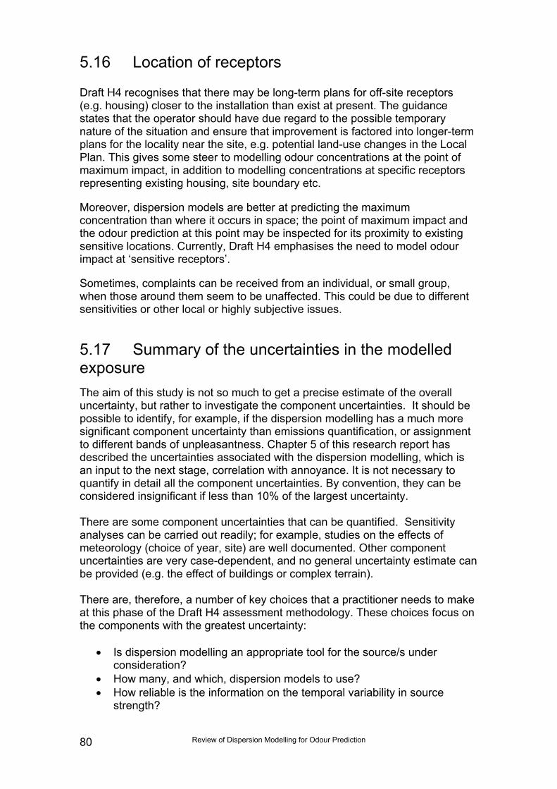
Review of Dispersion Modelling for Odour Prediction80
5.16 Location of receptors
Draft H4 recognises that there may be long-term plans for off-site receptors(e.g. housing) closer to the installation than exist at present. The guidancestates that the operator should have due regard to the possible temporarynature of the situation and ensure that improvement is factored into longer-termplans for the locality near the site, e.g. potential land-use changes in the LocalPlan. This gives some steer to modelling odour concentrations at the point ofmaximum impact, in addition to modelling concentrations at specific receptorsrepresenting existing housing, site boundary etc.
Moreover, dispersion models are better at predicting the maximumconcentration than where it occurs in space; the point of maximum impact andthe odour prediction at this point may be inspected for its proximity to existingsensitive locations. Currently, Draft H4 emphasises the need to model odourimpact at ‘sensitive receptors’.
Sometimes, complaints can be received from an individual, or small group,when those around them seem to be unaffected. This could be due to differentsensitivities or other local or highly subjective issues.
5.17 Summary of the uncertainties in the modelledexposureThe aim of this study is not so much to get a precise estimate of the overalluncertainty, but rather to investigate the component uncertainties. It should bepossible to identify, for example, if the dispersion modelling has a much moresignificant component uncertainty than emissions quantification, or assignmentto different bands of unpleasantness. Chapter 5 of this research report hasdescribed the uncertainties associated with the dispersion modelling, which isan input to the next stage, correlation with annoyance. It is not necessary toquantify in detail all the component uncertainties. By convention, they can beconsidered insignificant if less than 10% of the largest uncertainty.
There are some component uncertainties that can be quantified. Sensitivityanalyses can be carried out readily; for example, studies on the effects ofmeteorology (choice of year, site) are well documented. Other componentuncertainties are very case-dependent, and no general uncertainty estimate canbe provided (e.g. the effect of buildings or complex terrain).
There are, therefore, a number of key choices that a practitioner needs to makeat this phase of the Draft H4 assessment methodology. These choices focus onthe components with the greatest uncertainty:
• Is dispersion modelling an appropriate tool for the source/s underconsideration?
• How many, and which, dispersion models to use?• How reliable is the information on the temporal variability in source
strength?
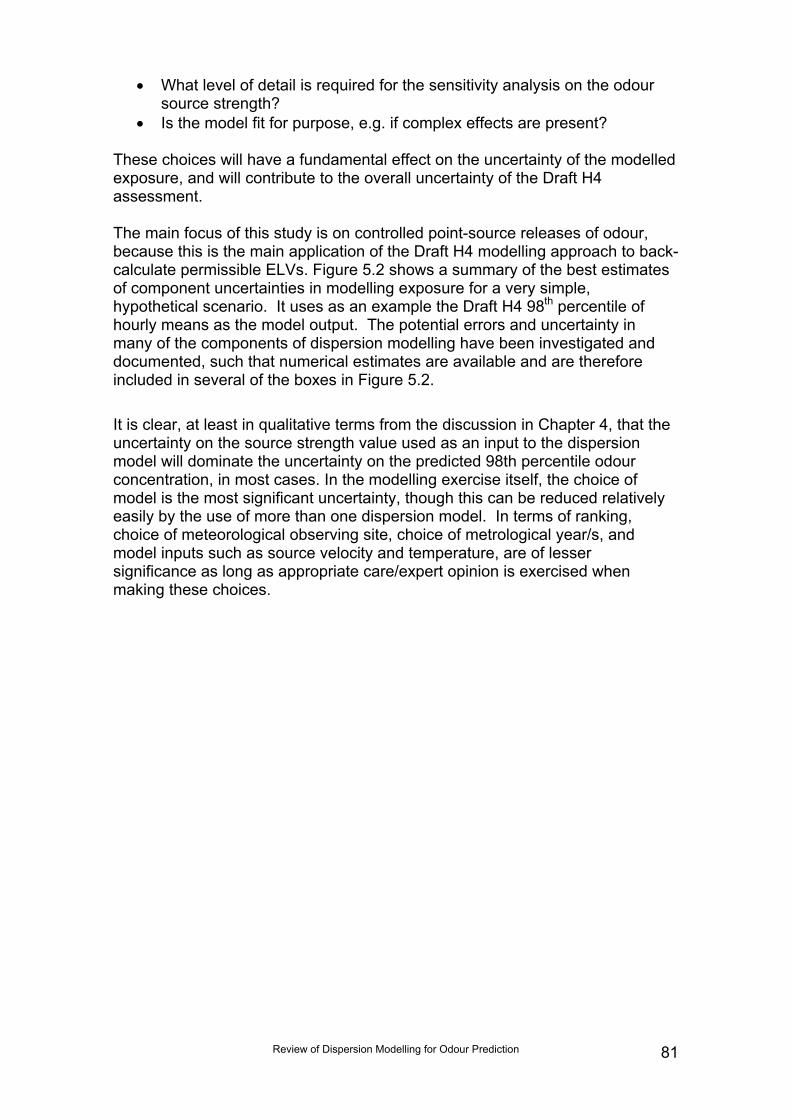
Review of Dispersion Modelling for Odour Prediction 81
• What level of detail is required for the sensitivity analysis on the odoursource strength?
• Is the model fit for purpose, e.g. if complex effects are present?
These choices will have a fundamental effect on the uncertainty of the modelledexposure, and will contribute to the overall uncertainty of the Draft H4assessment.
The main focus of this study is on controlled point-source releases of odour,because this is the main application of the Draft H4 modelling approach to back-calculate permissible ELVs. Figure 5.2 shows a summary of the best estimatesof component uncertainties in modelling exposure for a very simple,hypothetical scenario. It uses as an example the Draft H4 98th percentile ofhourly means as the model output. The potential errors and uncertainty inmany of the components of dispersion modelling have been investigated anddocumented, such that numerical estimates are available and are thereforeincluded in several of the boxes in Figure 5.2.
It is clear, at least in qualitative terms from the discussion in Chapter 4, that theuncertainty on the source strength value used as an input to the dispersionmodel will dominate the uncertainty on the predicted 98th percentile odourconcentration, in most cases. In the modelling exercise itself, the choice ofmodel is the most significant uncertainty, though this can be reduced relativelyeasily by the use of more than one dispersion model. In terms of ranking,choice of meteorological observing site, choice of metrological year/s, andmodel inputs such as source velocity and temperature, are of lessersignificance as long as appropriate care/expert opinion is exercised whenmaking these choices.
82
Figure 5.exposure
Uncertaintiesassociatedwith quality ofinput data:dominated by
Unc
erta
intie
s du
e to
“Ext
erna
l Fac
tors
”U
ncer
tain
ties
due
to “I
nter
nal F
acto
rs’
Odour release value (OUEs-1
(See Figure 4.2 and Chapter4)
Representivity of metobserving station: +20%
Representivity of met data year:+30% with 5 years of met data
Review of Dispersion Modelling for Odour Prediction
2 Summary of the estimated uncertainties in the modelled value:hypothetical simple scenario
Atmospheric processes e.g.deposition, washout, chemistry:very case-dependent
Temporal variability inemissions – very case-dependent
Terrain & surface roughness:resolution of mapped grids –+400%
Buildings: + 300%
Release conditions e.g. v, T,discharge geometry: + 12%
Receptor locations andheights for modellingexposure: +50%
uncertainty onodour releasevalue?
Uncertaintiesassociatedwith the modelalgorithms :more robustvalidation forsimple cases,e.g. pointsources
Modelsensitivity toinputparameters
Uncertainty onmodelled 98th
percentile value(for Draft H4approach)
Correlationwithannoyancelevel: DraftH4 IOES
Representation of source:+10% for this single pointsource, case dependent forother source types
Model type/version: + 200%if two new-generation modelsused
Model choice: unknownuncertainty in relation tomodel which was used toset IOES
Review of Dispersion Modelling for Odour Prediction 83
6 Phase III: Correlation withAnnoyance
6.1 Overview of this phase
The PPC Regulations include in their definition of pollution “emissions as aresult of human activity which…cause offence to any human senses” and theEnvironment Agency has given special consideration as to how the endpoint ofodour “offence” may be anticipated, measured and assessed in terms ofannoyance.
The preceding phases – quantifying an odour release value and then using thisas input to an atmospheric dispersion model – provide us with a prediction ofthe odour exposure at the receptor location. This exposure is given in terms ofthe 98 percentile of 1-hour average concentrations (C98, 1-hour)#.However, knowing the exposure, on its own, is not sufficient. From thispredicted odour exposure, a view must be formed on whether it is likely tocause odour annoyance◊. This can be done by establishing what is, in effect,a calibration curve: the basis for establishing this correlation is the empiricalrelationship between odour exposure (measured, or more usually, modelled)and annoyance (measured by a community survey). The details are given inProject 2 of this cluster.
The approach used by the Environment Agency in Draft H4 when determiningApplications/Variations under PPC is to derive from this empiricalepidemiological relationship a numerical modelling guideline standard to definein numerical terms its “benchmark” criterion of “no reasonable cause forannoyance”*. The odour exposure predicted by dispersion modelling iscompared to the numerical modelling guideline standard to judge whetherannoyance is likely to occur. The aim of odour control is therefore to ensurethere is “no reasonable cause for annoyance”.
# This encompasses (in a different form) the frequency, intensity, duration and location aspectsof the FIDOL factors described earlier in Chapter 3; the offensiveness (i.e. unpleasantness)component is based on a consensus judgement for that particular type of installation or odour.
◊ This difference between odour exposure and odour annoyance is crucial. Similarly, it isimportant to emphasise the technical differences between annoyance and nuisance. Thischapter concerns itself only with odour exposure and annoyance.
* For the purposes of the PPC Regulations, the Agency deems the point at which pollution in theform of offence to the sense of smell is occurring to be the point at which there is “reasonablecause for annoyance”. The “benchmark” criterion of “no reasonable cause for annoyance” doesnot necessarily equate to no complaints - it is designed to be a level of exposure that a highproportion of the exposed population, with normal sense of smell, finds “acceptable” on a long-term basis. Conversely, the lack of complaint should not necessarily imply the absence of anodour problem, as there will be an underlying level of annoyance before complaints are made
Review of Dispersion Modelling for Odour Prediction84
Draft H4 allows two routes to making this comparison with its benchmark:
• The first route is to derive a bespoke odour exposure guideline standardfrom an industry-specific dose-response relationship carried out inEngland and Wales.
• The alternative is to use the default “Indicative Odour ExposureStandards” that have been derived by the Environment Agency from thedose-response relationship established for a community living around alivestock installation in the Netherlands. The assumption has been madethat the results of this study can be applied generically to otherapplications with certain adjustments and factors applied (see Section6.3 for more details).
The Indicative Odour Exposure Standards approach clearly has an additionallayer of uncertainty compared to the approach of deriving a bespoke guidelinestandard. For this reason the two approaches are looked at separately in thefollowing sections.
6.2 Bespoke odour exposure guideline standardsderived from industry-specific dose-response studies
6.2.1 Summary of the component uncertainties in industry-specific guidelines
The Environment Agency’s Draft H4 guidance allows* PPC applicants to deriveindustry-specific dose-response relationships between annoyance and 98%concentrations (1-hour average), as an alternative to using the indicativeexposure standards provided (which are effectively “default values”). At the timeof writing, the Environment Agency had not received any applications inEngland and Wales that used bespoke industry-specific dose-responserelationships.
In order to investigate the uncertainty in the correlation of odour exposure withannoyance based on such a dose-response study, it is necessary to examinethe component steps in the study. These can be summarised as follows:
i. A suitable field-study candidate is identified. The installation should berepresentative of the industry or odour type in question, and thesurrounding community should be representative of the wider populationto which it is going to be applied (e.g. the whole sector).
ii. Odour emissions from the installation are measured at source bydynamic dilution olfactometry. Then, atmospheric dispersion modelling is
* It is perhaps worth noting that in the New Zealand guidance (Ministry for theEnvironment New Zealand 2003) that post-dates the draft H4, a stronger steer is given: industryis expected to derive their own dose-response relationships and it is made clear that theindicative guideline values provided there are temporary and only for use until such studieshave been completed.
Review of Dispersion Modelling for Odour Prediction 85
carried out to predict the surrounding ground-level concentrations (C98, 1-
hour). iii. Zones of distinct odour exposure levels are identified and the percentage
of people annoyed in each zone is estimated using questionnaires and arandom sample of addresses falling in each zone.
iv. The percentage of “annoyed” respondents in the sample is then plottedagainst the exposure band to establish a dose-effect relationship for theparticular type of installation/odour. The dose-response curve, whichtends to be S-shaped, is fitted by regression (see Figure 3.2 for anexample).
v. A suitable level of annoyance – which can be chosen based on policygrounds or technical grounds – is selected and the corresponding level ofodour exposure is read-off from the curve. This 98% concentrations (1-hour average) is the bespoke odour exposure guideline standard.
Each of these steps contains component uncertainties that will go to make upthe uncertainty in the bespoke odour exposure guideline standard that is finallyderived. These are summarised in Figure 6.1, and the information available onthese component uncertainties is discussed in the following sections.
6.2.2 Uncertainties associated with the application of the dose-response study
Temporal uncertainties
The main temporal uncertainty is where the period of the dose-response studyis not wholly representative of the period of interest. For example, it is knownthat most odour complaints are received during the summer months; this can bebecause high temperatures favour odour formation at source, but it is alsobecause people spend more time in their gardens and with their windows open.The selection of an appropriate duration for the study depends on many of thesame factors used to select the duration of a representative ambient air qualitymonitoring campaign; these are discussed in Environment Agency TechnicalGuidance Note M8 (Environment Agency 2006). Careful planning is needed tobe ensure the study period encompasses (or even focuses on) those plantconditions and meteorological conditions that are expected to lead to odourepisodes.
This uncertainty component will be specific to the particular dose-responsestudy being carried out; it is difficult to put any kind of general figure on itsuncertainty. In practice, the approach taken is likely to be one that ensures thiscomponent uncertainty is minimised – by ensuring that such studies adhere torobust Environment Agency technical guidance – and then considerednegligible.
Review of Dispersion Modelling for Odour Prediction86
Spatial uncertainties
Due to the effort, complexity and cost of a bespoke dose-response study, it isnot likely that these will be carried out for every installation. Certainly theexpectation of regulators in Australia and New Zealand is that such studies willrequire central funding or will be carried out by operators on a sector-widebasis. It is important therefore that the installation chosen for the study, and theodours it releases, are representative of that sector as a whole. Uncertainty willbe greater where the sector encompasses many different types of plant andodour; it will be smaller where the sector focuses on a narrow band ofprocesses and odours with similar characteristics. Regarding differences inodour unpleasantness between some types of installation, Project 2 in thiscluster considers this issue in more detail, discussing whether the grouping ofsome industries/sectors needs to be broken down further to account for this(Environment Agency 2007b).
A further contributor to the spatial uncertainty will be how representative are thecommunity surrounding the installation chosen for the dose-response study.Project 2 in this cluster discusses the differences in annoyance response*
between people who are used to a type of odour and those who are not; andalso those people who have some kind of economic relationship with theinstallation – for example, they are employed there. In addition, other ambientstressors, such as noise, dust and crowding can influence the response(Environment Agency 2007b, see Figure 3.1). These factors can lead tosignificant differences between the annoyance response to a given odourexposure at the study location and the responses at other installations in thatsector at different geographical locations. This is emphasised in New Zealandguidance (Ministry for the Environment 2002, 2003) which recognises that incommunity response-based studies an odour-modelling guideline is determinedfor a particular site based on population annoyance data, and therefore is basedon the tolerance of an existing community to an existing industrial or tradeactivity. The tolerance of an existing community to a new industrial or tradeactivity, or increased odour emissions from an existing activity, would beexpected to be lower. The New Zealand guidance therefore applies a tolerancefactor to reduce (i.e. make more stringent) the odour-modelling guideline torepresent the lower tolerance of existing communities to new sources of odour.Based on case studies, the tolerance factor was estimated at approximately 2–5.
Again, it is not possible to place any numerical estimates of the magnitude ofthese situation-specific uncertainties, but practitioners must make themselvesaware of the possible importance and form a qualitative view on the significanceof this component of uncertainty. Robust Environment Agency technical
* The factors affecting human response to odour, and the relationship betweenperception, cognitive appraisal and behavioural responses, are also summarised in Appendix 2of Draft H4 Part 1, and described in detail in Environment Agency R&D Report P4-095/TR(Environment Agency 2002b). Draft H4 recognises that the setting of odour benchmarks is stilla developing field. The response to exposure to an odour is primarily subjective – how strong itis, what it smells like, and in what context. There can be large differences between individualsin terms of their sensitivity, likes and dislikes and attitudes to exposure.

Review of Dispersion Modelling for Odour Prediction 87
guidance on carrying out sector-wide dose-response studies will help minimisethis component uncertainty.
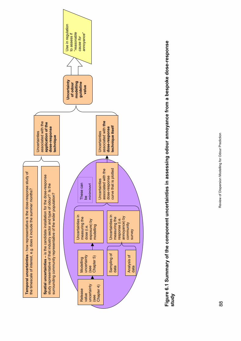
Rev
iew
of D
ispe
rsio
n M
odel
ling
for O
dour
Pre
dict
ion
88Figu
re 6
.1 S
umm
ary
of th
e co
mpo
nent
unc
erta
intie
s in
ass
essi
ng o
dour
ann
oyan
ce fr
om a
bes
poke
dos
e-re
spon
sest
udy
Unc
erta
inty
of o
dour
mod
ellin
ggu
idel
ine
valu
e
Tem
pora
l unc
erta
intie
s - h
ow re
pres
enta
tive
is th
e do
se-re
spon
se s
tudy
of
the
times
cale
of i
nter
est,
e.g.
doe
s it
incl
ude
the
sum
mer
mon
ths?
Spat
ial u
ncer
tain
ties
– is
the
cand
idat
e in
stal
latio
n fo
r the
dos
e-re
spon
sest
udy
repr
esen
tativ
e of
that
indu
stry
sec
tor a
nd ty
pe o
f odo
ur?
Is th
esu
rroun
ding
com
mun
ity re
pres
enta
tive
of th
e w
ider
pop
ulat
ion?
Unc
erta
intie
sas
soci
ated
with
the
dose
-res
pons
ecu
rve
that
is p
lotte
d
Unc
erta
intie
sas
soci
ated
with
the
appl
icat
ion
of th
edo
se-r
espo
nse
tech
niqu
e
Unc
erta
intie
sas
soci
ated
with
the
dose
-res
pons
ete
chni
que
itsel
f
Mod
ellin
gun
certa
inty
(see
Cha
pter
5)
Thes
e ca
nbe m
inim
ised
Use
in re
gula
tion
to a
sses
s if
“reas
onab
leca
use
for
anno
yanc
e”
Unc
erta
intie
s in
mea
surin
g th
ere
spon
se (i
.e.
anno
yanc
e) b
yco
mm
unity
surv
ey
Unc
erta
intie
s in
mea
surin
g th
edo
se (i
.e.
expo
sure
) by
mod
ellin
g
Rel
ease
valu
eun
certa
inty
(see
Cha
pter
4)
Sam
plin
g of
data
Ana
lysi
s of
data
Review of Dispersion Modelling for Odour Prediction 89
6.2.3 Uncertainties associated with the dose-response studytechnique itself
The odour modelling guideline is read off from a dose-response curve,essentially a calibration curve, established by plotting two parameters:
• the odour exposure – the predicted ground-level concentrations (C98, 1-
hour) in the surrounding areas; and
• the odour response – the percentage of people annoyed in each zoneThe odour exposure values are obtained by atmospheric dispersion modellingof the source odour release value for the installation chosen for the study. Allthe release value and modelling uncertainties described in Chapters 4 and 5 willtherefore contribute.The odour response values are obtained from a community survey. Zones ofdistinct odour exposure levels are identified around the installation and thepercentage of people annoyed in each zone is obtained from questionnairesand a random sample of addresses falling in each zone. A well established VDImethodology (VDI 1997) exists for this.No studies in England or Wales have yet been carried out for PPC regulatorypurposes, so information on the likely uncertainties to be expected have to bedrawn from studies carried out elsewhere. For the dataset from a study arounda Dutch piggery*, Van Harreveld (2004) describes how regression fitting an S-shaped curve to these data showed a strong correlation (r>0.9) betweenmodelled exposure and annoyance. A level of 10% annoyed was chosen as thelowest level that would be statistically significant, based on the “backgroundnoise” for measurement of annoyance using questionnaires plus two times thestandard deviation. The level of 10% annoyance to pig odours correlated withan exposure (C98, 1-hour) of 1.3 ouE m-3 and this was used for the basis for settingan odour modelling guideline of 1.5 ouE m-3.The dose response curve is, essentially, a calibration curve for estimating avalue of X from Y. The uncertainty on this estimate can be obtained bycalculating the “inverse confidence limits”, which takes account of theuncertainty in the position of the calibration line itself and also the fact that themeasured value of Y is subject to some uncertainty. The standard deviation ofthe estimate of X from Y, for example the odour exposure value correspondingto 10% annoyance, is given by an equation. This is described in a Royal Societyof Chemistry Technical Brief (2006), which also gives macro programs forcarrying out the calculation.The original data from the Dutch study described above were not available forthis study. It was not possible (or within the scope of this literature review) to re-analyse the original data and carry out statistical analysis, so no estimate isavailable for the uncertainty in the derived modelling guideline. It isrecommended that the Environment Agency should strengthen the technicalguidance given in Draft H4 to require this uncertainty to be calculated for any
* This study was used for the data underpinning the Draft H4 Indicative Odour ExposureStandards (see Section 6.3) and also the Irish EPA odour exposure criteria for livestock odours.
Review of Dispersion Modelling for Odour Prediction90
bespoke odour modelling guidelines produced from sector-specific dose-response studies.
6.3 Using default Indicative Odour ExposureStandards
6.3.1 Background to the Summary Indicative Odour ExposureStandards
The Environment Agency recognises the reality of the situation as it currentlyexists – no bespoke dose-response studies have been carried out in Englandand Wales for PPC regulatory purposes and there is likely to be a time lagbetween issuing strong guidance on this being the favoured route, and suchstudies being completed to provide sector-specific odour exposure modellingstandards. Also, such community dose-response studies do require a definableodour source and an existing community with sufficient population density torepresent a suitable case study. This may not always be possible.To fill this gap the Environment Agency developed, for Draft H4, default“Indicative Odour Exposure Standards” that were derived from the relationshipestablished between ground-level odour concentration and odour annoyance fora sample of test subjects living around a livestock installation in theNetherlands. These “default” exposure criteria are set as a 98-percentile, 1-houraverage concentration (C98, 1-hour) of 1.5, 3.0 or 6.0 ouE m-3 for high, medium andlow categories of odour unpleasantness, respectively.The assumption was made that the results of this study could be appliedgenerically to other applications with certain adjustments and factors applied.For this reason, the use of Indicative Odour Exposure Standards to assess ifthere is “reasonable cause for annoyance” has an additional layer of uncertaintycompared to the approach of deriving a bespoke guideline standard. Thebackground to developing the Indicative Odour Exposure Standards isdescribed below along with a discussion of these additional uncertainties.The derivation of the Indicative Odour Exposure Standards is described in detailin the earlier Environment Agency Report P4-095 Assessment of CommunityResponse to Odorous Emissions (Environment Agency 2002b), which formedthe main background work for Draft H4. As discussed earlier, the dataset thatformed the main underpinning for the proposed values was collected in theNetherlands for livestock odours (Bongers et al. 2001) as specific data forEngland and Wales were not available#. (This data set was also used by theIrish EPA as a starting point to derive odour exposure criteria for livestockodours.) In brief, odour emissions from a piggery were measured at source by
# The Environment Agency research noted that, ideally, the dose-effectrelationship for UK citizens in UK conditions should be assessed experimentallyto confirm the findings obtained abroad, but as of date this has not been carriedout.
Review of Dispersion Modelling for Odour Prediction 91
dynamic dilution olfactometry, then modelled to predict the surrounding ground-level concentrations (C98, 1-hour). Zones of distinct odour exposure levels wereidentified and the percentage of people annoyed in each zone was estimatedusing questionnaires and a random sample of addresses falling in each zone.The percentage of “annoyed” respondents in the sample was then plottedagainst the exposure band to establish a dose-effect relationship for livestockodours. Regression fitting of an S-shaped curve showed a strong correlation(r>0.9) between modelled exposure and annoyance. A level of 10% annoyedwas chosen as the lowest level that would be statistically significant, based onthe “background noise” for measurement of annoyance using questionnairesplus two times the standard deviation.For the general public, the level of 10% annoyance to pig odours correlated withan exposure (C98, 1-hour) of 1.3 ouE m-3 and this was used for the basis of themost stringent Draft H4 indicative criteria, for high offensiveness (i.e.unpleasant) odours, of 1.5 ouE m-3.The earlier Environment Agency research suggested that it would be preferableto use the measurement of annoyance potential to characterise odouremissions, rather than using ouE s-1 alone, for input to the dispersion modellingand comparison with the percentage annoyed respondents to establish a dose-effect relationship. This would allow the true effect of hedonic tone,unpleasantness and odour character to be included in the relationship fordifferent types of odour. However, a laboratory method for measuringannoyance potential had not then been developed, so it was proposed thatexisting rank-order data for industrial odours (as shown in Table A1.1 of DraftH4) should be the basis for assigning different odour types into a simple three-band categorisation:
• High odour annoyance potential (e.g. animal rendering, fat and greaseprocessing, etc.)
• Medium odour annoyance potential – all odours not in categories High orLow.
• Low odour annoyance potential (e.g. bakeries, coffee roaster)
The particular numerical guidelines that were assigned in Draft H4 to theindicative criteria for odours of medium unpleasantness and odours of lowunpleasantness were arrived at as follows.For residents in areas where pig odours were a common feature, the 10%annoyed level corresponded to an exposure of (C98, 1-hour) of 3.2 ouE m-3 and thisvalue was used for the basis of the Draft H4 indicative criteria for mildlyunpleasant odours of 3.0 ouE m-3. The most lenient Draft H4 indicative criterionof 6 ouE m-3, assigned to “less offensive” odours, was based on 10% annoyedof respondents who worked in agriculture (corresponding to 13 ouE m-3)combined with data from a dozen dose-effect studies for industrial sectors in theNetherlands where the 10% annoyed level corresponded with approximately <5ouE m-3. In addition, inspection of a number of consultancy projects indicatedthat between 90 and 95% of complaints registered for wastewater treatmentand solid waste management occurred in the exposure range of 5 to 10 ouE m-3.A summary of how the Indicative Odour Exposure Standards were derived fromthe Dutch results is shown in Table 6.1.
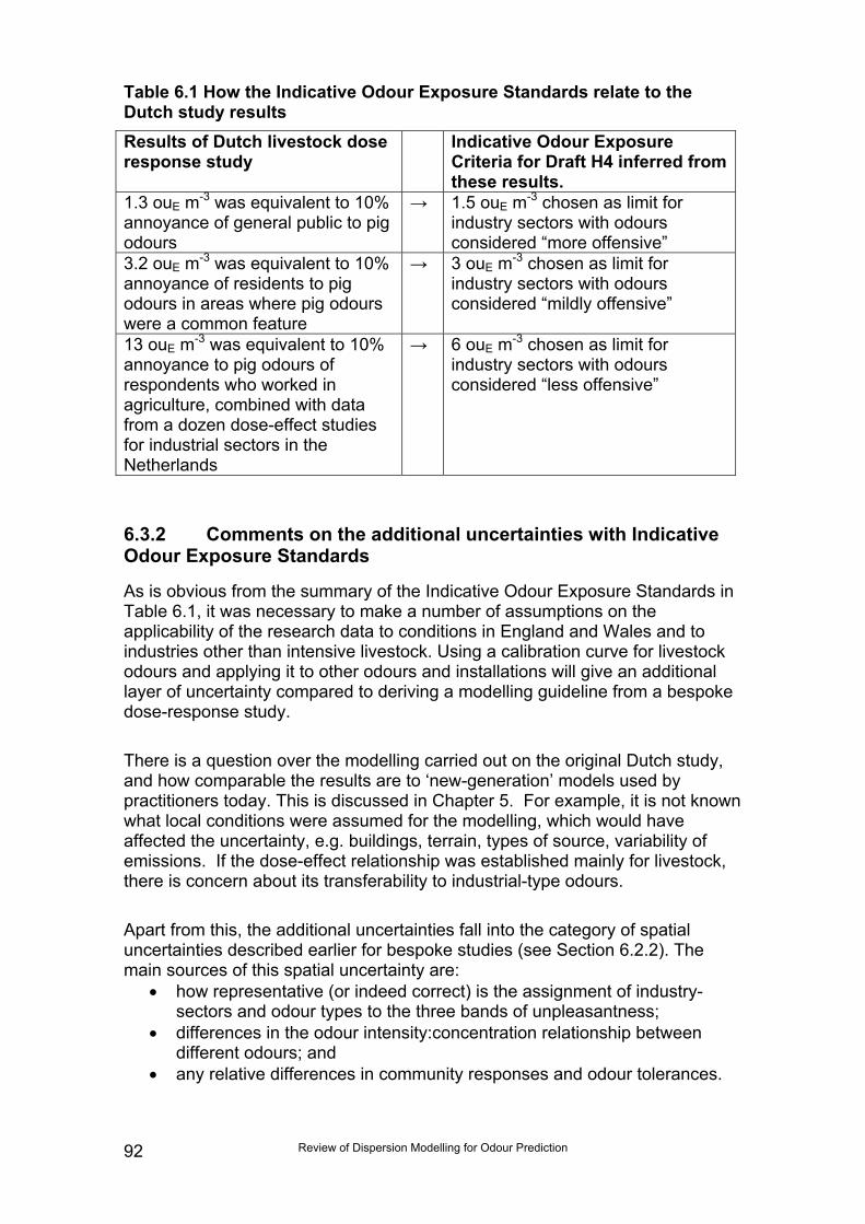
Review of Dispersion Modelling for Odour Prediction92
Table 6.1 How the Indicative Odour Exposure Standards relate to theDutch study resultsResults of Dutch livestock doseresponse study
Indicative Odour ExposureCriteria for Draft H4 inferred fromthese results.
1.3 ouE m-3 was equivalent to 10%annoyance of general public to pigodours
→ 1.5 ouE m-3 chosen as limit forindustry sectors with odoursconsidered “more offensive”
3.2 ouE m-3 was equivalent to 10%annoyance of residents to pigodours in areas where pig odourswere a common feature
→ 3 ouE m-3 chosen as limit forindustry sectors with odoursconsidered “mildly offensive”
13 ouE m-3 was equivalent to 10%annoyance to pig odours ofrespondents who worked inagriculture, combined with datafrom a dozen dose-effect studiesfor industrial sectors in theNetherlands
→ 6 ouE m-3 chosen as limit forindustry sectors with odoursconsidered “less offensive”
6.3.2 Comments on the additional uncertainties with IndicativeOdour Exposure Standards
As is obvious from the summary of the Indicative Odour Exposure Standards inTable 6.1, it was necessary to make a number of assumptions on theapplicability of the research data to conditions in England and Wales and toindustries other than intensive livestock. Using a calibration curve for livestockodours and applying it to other odours and installations will give an additionallayer of uncertainty compared to deriving a modelling guideline from a bespokedose-response study.
There is a question over the modelling carried out on the original Dutch study,and how comparable the results are to ‘new-generation’ models used bypractitioners today. This is discussed in Chapter 5. For example, it is not knownwhat local conditions were assumed for the modelling, which would haveaffected the uncertainty, e.g. buildings, terrain, types of source, variability ofemissions. If the dose-effect relationship was established mainly for livestock,there is concern about its transferability to industrial-type odours.
Apart from this, the additional uncertainties fall into the category of spatialuncertainties described earlier for bespoke studies (see Section 6.2.2). Themain sources of this spatial uncertainty are:
• how representative (or indeed correct) is the assignment of industry-sectors and odour types to the three bands of unpleasantness;
• differences in the odour intensity:concentration relationship betweendifferent odours; and
• any relative differences in community responses and odour tolerances.
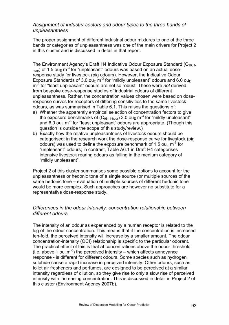
Review of Dispersion Modelling for Odour Prediction 93
Assignment of industry-sectors and odour types to the three bands ofunpleasantness
The proper assignment of different industrial odour mixtures to one of the threebands or categories of unpleasantness was one of the main drivers for Project 2in this cluster and is discussed in detail in that report.
The Environment Agency’s Draft H4 Indicative Odour Exposure Standard (C98, 1-
hour) of 1.5 ouE m-3 for “unpleasant” odours was based on an actual dose-response study for livestock (pig odours). However, the Indicative OdourExposure Standards of 3.0 ouE m-3 for “mildly unpleasant” odours and 6.0 ouEm-3 for “least unpleasant” odours are not so robust. These were not derivedfrom bespoke dose-response studies of industrial odours of differentunpleasantness. Rather, the concentration values chosen were based on dose-response curves for receptors of differing sensitivities to the same livestockodours, as was summarised in Table 6.1. This raises the questions of:a) Whether the apparently empirical selection of concentration factors to give
the exposure benchmarks of (C98, 1-hour) 3.0 ouE m-3 for “mildly unpleasant”and 6.0 ouE m-3 for “least unpleasant” odours are appropriate. (Though thisquestion is outside the scope of this study/review.)
b) Exactly how the relative unpleasantness of livestock odours should becategorised: in the research work the dose-response curve for livestock (pigodours) was used to define the exposure benchmark of 1.5 ouE m-3 for“unpleasant” odours; in contrast, Table A6.1 in Draft H4 categorisesintensive livestock rearing odours as falling in the medium category of“mildly unpleasant”.
Project 2 of this cluster summarises some possible options to account for theunpleasantness or hedonic tone of a single source (or multiple sources of thesame hedonic tone – evaluation of multiple sources of different hedonic tonewould be more complex. Such approaches are however no substitute for arepresentative dose-response study.
Differences in the odour intensity: concentration relationship betweendifferent odours
The intensity of an odour as experienced by a human receptor is related to thelog of the odour concentration. This means that if the concentration is increasedten-fold, the perceived intensity will increase by a smaller amount. The odourconcentration-intensity (OCI) relationship is specific to the particular odorant.The practical effect of this is that at concentrations above the odour threshold(i.e. above 1 ouEm-3) the perceived intensity – which affects annoyanceresponse - is different for different odours. Some species such as hydrogensulphide cause a rapid increase in perceived intensity. Other odours, such astoilet air fresheners and perfumes, are designed to be perceived at a similarintensity regardless of dilution, so they give rise to only a slow rise of perceivedintensity with increasing concentration. This is discussed in detail in Project 2 ofthis cluster (Environment Agency 2007b).
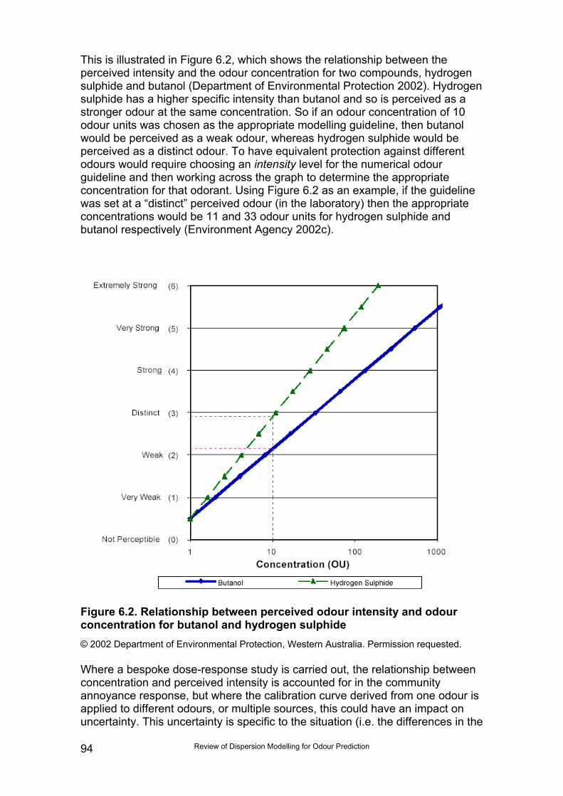
Review of Dispersion Modelling for Odour Prediction94
This is illustrated in Figure 6.2, which shows the relationship between theperceived intensity and the odour concentration for two compounds, hydrogensulphide and butanol (Department of Environmental Protection 2002). Hydrogensulphide has a higher specific intensity than butanol and so is perceived as astronger odour at the same concentration. So if an odour concentration of 10odour units was chosen as the appropriate modelling guideline, then butanolwould be perceived as a weak odour, whereas hydrogen sulphide would beperceived as a distinct odour. To have equivalent protection against differentodours would require choosing an intensity level for the numerical odourguideline and then working across the graph to determine the appropriateconcentration for that odorant. Using Figure 6.2 as an example, if the guidelinewas set at a “distinct” perceived odour (in the laboratory) then the appropriateconcentrations would be 11 and 33 odour units for hydrogen sulphide andbutanol respectively (Environment Agency 2002c).
Figure 6.2. Relationship between perceived odour intensity and odourconcentration for butanol and hydrogen sulphide© 2002 Department of Environmental Protection, Western Australia. Permission requested.
Where a bespoke dose-response study is carried out, the relationship betweenconcentration and perceived intensity is accounted for in the communityannoyance response, but where the calibration curve derived from one odour isapplied to different odours, or multiple sources, this could have an impact onuncertainty. This uncertainty is specific to the situation (i.e. the differences in the
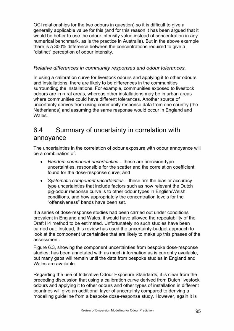
Review of Dispersion Modelling for Odour Prediction 95
OCI relationships for the two odours in question) so it is difficult to give agenerally applicable value for this (and for this reason it has been argued that itwould be better to use the odour intensity value instead of concentration in anynumerical benchmark, as is the practice in Australia). But in the above examplethere is a 300% difference between the concentrations required to give a“distinct” perception of odour intensity.
Relative differences in community responses and odour tolerances.
In using a calibration curve for livestock odours and applying it to other odoursand installations, there are likely to be differences in the communitiessurrounding the installations. For example, communities exposed to livestockodours are in rural areas, whereas other installations may be in urban areaswhere communities could have different tolerances. Another source ofuncertainty derives from using community response data from one country (theNetherlands) and assuming the same response would occur in England andWales.
6.4 Summary of uncertainty in correlation withannoyanceThe uncertainties in the correlation of odour exposure with odour annoyance willbe a combination of:
• Random component uncertainties – these are precision-typeuncertainties, responsible for the scatter and the correlation coefficientfound for the dose-response curve; and
• Systematic component uncertainties – these are the bias or accuracy-type uncertainties that include factors such as how relevant the Dutchpig-odour response curve is to other odour types in English/Welshconditions, and how appropriately the concentration levels for the“offensiveness” bands have been set.
If a series of dose-response studies had been carried out under conditionsprevalent in England and Wales, it would have allowed the repeatability of theDraft H4 method to be estimated. Unfortunately no such studies have beencarried out. Instead, this review has used the uncertainty-budget approach tolook at the component uncertainties that are likely to make up this phases of theassessment.Figure 6.3, showing the component uncertainties from bespoke dose-responsestudies, has been annotated with as much information as is currently available,but many gaps will remain until the data from bespoke studies in England andWales are available.
Regarding the use of Indicative Odour Exposure Standards, it is clear from thepreceding discussion that using a calibration curve derived from Dutch livestockodours and applying it to other odours and other types of installation in differentcountries will give an additional layer of uncertainty compared to deriving amodelling guideline from a bespoke dose-response study. However, again it is

Review of Dispersion Modelling for Odour Prediction96
not possible to place any numerical estimates of the magnitude of this additionallayer of uncertainty, as it is situation-specific. For a livestock installation theadditional layer of uncertainty might be expected to be small. For other, verydifferent, odours or installations the leap of faith is wider and the additionaluncertainty may be much larger. Practitioners must make themselves aware ofthe possible importance and form a qualitative view on the significance of thiscomponent of uncertainty.
On the positive side, the level of annoyance measured by the survey in the NewZealand Technical Report (Ministry for the Environment 2002) was found to beconsistent with the odour dose-community-response curves reported byMiedema (1992). The dose-response curves, although developed for otherindustries and using a Dutch community response, appeared to be valid for pulpmill odours in New Zealand.
In terms of the future outlook for using Indicative Odour Exposure Standardscompared to deriving a modelling guideline from a bespoke dose-responsestudy, the Draft H4 guidance does state that the above benchmarks areindicative standards and that dose-effect studies in England and Wales areplanned. It also states elsewhere in the document that “the only realistic way ofestimating the actual level of annoyance in a particular community resultingfrom exposure is by carrying out dose-response studies locally”. However, DraftH4 appears much less explicit than the New Zealand guidance in highlightingthe “interim” nature of these generic-type odour guidelines and that they shouldideally be superseded by industry-specific guidelines developed from bespokedose-response studies. It is possible that some dose-response studies will beperformed around waste management facilities as part of a study into definingloss of amenity though odour carried out as part of Defra`s Waste ResearchR&D programme*. There is also a possibility of UK Water Industry Research(UKWIR) coordinating some studies around wastewater treatment plants tosupport the water industry in meeting the Defra Code of Practice on OdourNuisance from Sewage Treatment Works (Defra 2006).
* Details at http://www.defra.gov.uk/environment/waste/wip/research/index.htm
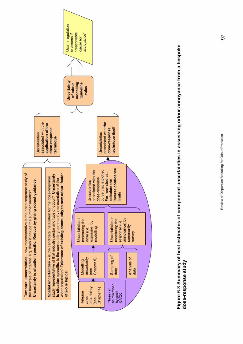
Rev
iew
of D
ispe
rsio
n M
odel
ling
for O
dour
Pre
dict
ion
97
Figu
re 6
.3 S
umm
ary
of b
est e
stim
ates
of c
ompo
nent
unc
erta
intie
s in
ass
essi
ng o
dour
ann
oyan
ce fr
om a
bes
poke
dose
-res
pons
e st
udy
Unc
erta
inty
of o
dour
mod
ellin
ggu
idel
ine
valu
e
Tem
pora
l unc
erta
intie
s - h
ow re
pres
enta
tive
is th
e do
se-re
spon
se s
tudy
of
the
times
cale
of i
nter
est,
e.g.
doe
s it
incl
ude
the
sum
mer
mon
ths?
Unc
erta
inty
is s
ituat
ion
spec
ific.
Red
uce
by g
ivin
g ro
bust
gui
danc
e.
Spat
ial u
ncer
tain
ties
– is
the
cand
idat
e in
stal
latio
n fo
r the
dos
e-re
spon
sest
udy
repr
esen
tativ
e of
that
indu
stry
sec
tor a
nd ty
pe o
f odo
ur?
Unc
erta
inty
is s
ituat
ion
spec
ific.
Is th
e su
rroun
ding
com
mun
ity re
pres
enta
tive
of th
ew
ider
pop
ulat
ion?
Tol
eran
ce o
f exi
stin
g co
mm
unity
to n
ew o
dour
: fac
tor
of 2
-5 is
typi
cal
Unc
erta
intie
sas
soci
ated
with
the
dose
-res
pons
ecu
rve
that
is p
lotte
d.Fo
r new
stu
dies
,ca
lcul
ate
the
inve
rse
conf
iden
celim
its
Unc
erta
intie
sas
soci
ated
with
the
appl
icat
ion
of th
edo
se-r
espo
nse
tech
niqu
e
Unc
erta
intie
sas
soci
ated
with
the
dose
-res
pons
ete
chni
que
itsel
f
Mod
ellin
gun
certa
inty
(see
Cha
pter
5)
Thes
e ca
nbe
min
imis
edby
goo
dQ
A/Q
C
Use
in re
gula
tion
to a
sses
s if
“reas
onab
leca
use
for
anno
yanc
e”
Unc
erta
intie
s in
mea
surin
g th
ere
spon
se (i
.e.
anno
yanc
e) b
yco
mm
unity
surv
ey
Unc
erta
intie
s in
mea
surin
g th
edo
se (i
.e.
expo
sure
) by
mod
ellin
g
Rel
ease
valu
eun
certa
inty
(see
Cha
pter
4)
Sam
plin
g of
data
Ana
lysi
s of
data
Review of Dispersion Modelling for Odour Prediction98
7 Phase IV: – Correlation withNegative Coping Behaviours(Nuisance and Complaints
7.1 Adverse outcomes of odour exposure –annoyance, nuisance, complaintsThe terms used to describe an odour’s potential to cause these adverse effects,and the terms describing the effects themselves (e.g. annoyance andnuisance), are explained in detail in Project 2 of this cluster. A summary of thetechnical differences between annoyance and nuisance is shown in Table 7.1,which is drawn from that project. It is helpful to read these terms in conjunctionwith Figure 3.1, which summarises the pathway from odour formation through tocomplaint.It is important to emphasise the technical differences between annoyance andnuisance: one major distinction is that annoyance occurs from an immediateexposure; nuisance on the other hand, is caused cumulatively, by repeatedevents of annoyance.Both, or either, annoyance and nuisance can lead to complaint action. Howevera lack of complaints does not necessarily prove there is no annoyance ornuisance. On the other hand, there needs to be an underlying level ofannoyance before complaints are generated.A complicating factor is that as well as the technical definition, nuisance is alsoa term in law (e.g. Statutory Nuisance). The definition of Statutory Nuisancecovers seven areas, and that which relates to odour is (s.79(1) EnvironmentalProtection Act (EPA) 1990):“any dust, steam, smell or other effluvia arising on industrial, trade or businesspremises and being prejudicial to health or a nuisance;”The legal use of nuisance has preceded the technical definition of nuisancedescribed here, which has only relatively recently been put forward andgenerally accepted. The EPA 1990 contains no technical definitions ofnuisance, such as maximum concentrations, frequencies or durations of odourin air.Any technical guidance can currently, therefore, only provide a method toassess nuisance against currently accepted technical criteria. Although it ishoped that these would also satisfy the legal definition of Statutory Nuisance forodour, it is ultimately only the Court that can make that decision.Although the extension of the Draft H4 methodology to predict nuisance orcompliant is beyond the scope of this literature review, a brief overview hasbeen given.

Review of Dispersion Modelling for Odour Prediction 99
Table 7.1. Proposed technical definition of annoyance and annoyancepotential (Van Harreveld 2001)Annoyancepotential
Annoyance potential is the attribute of a specific odour (or mixture ofodorants) to cause a negative appraisal in humans that requires copingbehaviour when perceived as an ambient odour in the living environment. Itis an attribute of an odour that can cause annoyance or nuisance.Annoyance potential indicates the magnitude of the ability of a specificodorant (mixture), relative to other odorants (mixtures), to causeannoyance in humans when repeatedly exposed in the living environmentto odours classified as ‘weak’ to ‘distinct odour’ on the scale of perceivedintensity (VDI 3882:1997, part 1).Whether annoyance potential of an odour does, or does not, causeannoyance (see below) depends on location and receptor factors.
Annoyance
Annoyance is the complex of human reactions that occurs as a resultof an immediate exposure to an ambient stressor (odour) that, onceperceived, causes negative cognitive appraisal that requires a degree ofcoping.Annoyance may, or may not, lead to nuisance and to complaint action.
Nuisance Nuisance is the cumulative effect on humans, caused by repeatedevents of annoyance over an extended period of time that leads tomodified or altered behaviour. This behaviour can be active (e.g.registering complaints, closing windows, keeping “odour diaries”, avoidinguse of the garden) or passive (only made visible by different behaviour intest situations, e.g. responding to questionnaires or different responses ininterviews). Odour nuisance can have a detrimental effect on our sense ofwell-being, and hence a negative effect on health. Nuisance occurs whenpeople are affected by an odour they can perceive in their livingenvironment (home, work-environment, recreation environment) and:i) the appraisal of the odour is negative;ii) the perception occurs repeatedly;iii) it is difficult to avoid perception of the odour; andiv) the odour is considered a negative effect on their well-being.
Nuisancepotential
Nuisance potential is the characteristic of an exposure situation, whichdescribes the magnitude of the nuisance that can be expected in a humanpopulation when exposed to an odour intermittently, but over an extendedperiod of time, in their living environment. Nuisance potential is a functionof many factors, such as the attributes of the odorant (mixture) in question,the frequency and dynamics of variation of the exposure (caused both atsource and as a result of atmospheric dispersion) and attributes of thespecific population that is exposed.
Nuisancesensitivity
Nuisance sensitivity is an attribute of a specific population (or anindividual) that indicates the propensity, relative to that of other individualsor populations, to experience nuisance when exposed to an odourintermittently, but over an extended period of time, in their livingenvironment.
Note: these definitions are from a technical perspective to enable a scientificunderstanding of the odour impact process. They are not legal or regulatorydefinitions (e.g. “no reasonable cause for annoyance”, or Statutory Nuisance).
Review of Dispersion Modelling for Odour Prediction100
7.2 Correlation of exposure with nuisance andcomplaints
Chapter 6 gave a detailed review of the uncertainties involved in the correlation ofpredicted odour exposure with annoyance. In theory, there is no reason why adose-response study could not be carried out using a different responsemeasurand – either nuisance or complaints. For nuisance, this would need to bepreceded by work to establish a method for measuring this parameter.
Dose response studies using complaints as the response measurand havebeen carried out in New Zealand and Australia, as described in Project 2 of thiscluster (Environment Agency 2007b). For example, the case study of a sewagetreatment facility in Sydney reviewed in the New Zealand Technical Report(Ministry for the Environment 2002) compared modelling results to areas ofvarying levels of complaint (as have most other similar investigations inAustralasia). The study established the link between observed levels ofcomplaint and percentile odour concentrations. The odour concentrations of theplant emissions were also measured using European methods, and ambientconcentrations were modelled using AUSPLUME and also using a wind tunnel.The community was alerted to the study by means of regular advertising, andso the community response may have been enhanced. Nevertheless, the studyfound that for sewage plant emissions, 99.5 percentile concentrations below 46ou m-3 were unlikely to lead to complaint. The equivalent certainty thresholdconcentration for this study was 5 ou m-3. The application of a 2 to 5 tolerancefactor to convert this to a guideline for assessing a proposed new activityindicates a modelling guideline for new sewage plants near sensitive areas inthe range of 1 to 3 ou m-3 (1-hour average, 99.5%, certainty).
Environment Agency report P4-079/TR/2 (2002c) concluded that for stackdischarges there are insufficient complaints data to validate the use ofdispersion models in the UK. The report states that to achieve validation, thereis a need to record the number of complaints from a single stack forapproximately 2 years. The report does however state that VDI 3883 Parts 1and 2 (questionnaire and community survey techniques for odour annoyanceassessment) have been recently employed to assess odour levels in the vicinityof a large industrial complex in Bedfordshire. The findings of this study couldprove useful to the review of uncertainties for Project 3.
Draft H4 recognises that complaint records are useful for looking at thedistribution of complaints around a source over a period of time. Identifyinglocations on a local map can show the footprint of a problem. Bureau Veritascarried out an odour dispersion modelling study in 2002 for a chipboardmanufacturing plant with a single stack. The ADMS3.1 model was used to plotcontours of the 99th and 98th percentile odour concentrations, where a peak-to-mean ratio of 10 was used to covert 1-hour mean model outputs to short-termfluctuations. It was found that the 98th percentile contours for 5 ouE m-3 andabove encompassed 16 complainants out of 27 households. It was found thatthe 99th percentile contours for 5 ouE m-3 and above encompassed 17complainants out of 27 households. It is noteworthy that the result of ADMS3.1fluctuation modelling did not give such a good agreement against thecomplaints records, with the model predicting a fluctuation concentration
Review of Dispersion Modelling for Odour Prediction 101
exceeding 5 ouE m-3 during at least 25 of the hours in the year at only 3 of the27 complaining properties. This arose from the inability of ADMS3.1 to modelbuilding downwash effects in conjunction with the concentration fluctuations.
A dispersion modelling study using AERMOD PRIME 4.4 for a refinery carriedout in 2006 predicted percentiles ranging from 90th to 100th, with an assessmentbenchmark of 1.5 ouE m-3 . It was found that the complaints records (whichspanned 3 years) matched the 99.9th and 100th percentile contours best. This isconsistent with the assumption that annoyance is represented by the 98th
percentile, and actual complaint action would be prompted by a higherfrequency of the odour at the benchmark concentration; there is an underlyinglevel of annoyance before complaints are made i.e. individuals experienceannoyance before they express this annoyance in the form of a complaint.
7.3 Complaints analysis
In contrast to the predictive approaches for assessing odour impact (e.g.dispersion modelling), direct approaches include complaints monitoring andcommunity assessment.
There are a number of factors which affect how and when complaints are made,and this makes it difficult to use complaints as an accurate reflection of theoverall level of annoyance in a community. There tends to be a ‘threshold’which has to be reached before initial complaints are made, but thereaftercomplaints may be made more readily. The number of people actuallyexperiencing the effects of annoyance caused by odour appears to be muchhigher than the number of registered complaints. In the Netherlands, theannoyance caused by odour is investigated by systematic year-on-year surveys(which disguise the purpose to avoid bias). Consideration should be given toestablishing surveys of this kind in the UK.
Comprehensive reviews of incidence of complaints in relation to odour exposurefor the UK are not available. However, in the UK, an increasing number ofcomplaints of odour have been received by many industries, and the generalconsensus of opinion is that it will continue to increase (Environment Agency2002c).
Complaints analysis is not covered by any standard method or recognisedprotocol. Complaints registration provides an insight into the prevalence of asymptom of odour annoyance, not in the prevalence of the annoyance itself.There are many factors at play that determine the ease or difficulty ofregistering a complaint.
7.4 Summary of uncertainty in correlation withnuisance and complaintsAlthough the extension of the Draft H4 methodology to predict nuisance orcompliant is beyond the scope of this literature review, a brief overview hasbeen given.
Review of Dispersion Modelling for Odour Prediction102
The legal use of nuisance has preceded the technical definition of nuisancedescribed here, which has only relatively recently been put forward andgenerally accepted. The EPA 1990 contains no technical definitions ofnuisance, such as maximum concentrations, frequencies or durations of odourin air. This would need to be addressed, together with a nuisance measurementmethodology, before any estimate of the uncertainty in the correlation withodour exposure could be made.Complaints are more usually measured directly by complaints monitoring, ratherthan predicted. However, dose response studies using complaints as theresponse measurand have been carried out in New Zealand and Australia, butusing different models to those in common use in the UK and using differentpercentiles to describe exposure.It would be safe to assume that the uncertainties in correlating predictedexposure with either nuisance or complaints levels would be considerablyhigher than for annoyance, due to the additional factors involved.
Review of Dispersion Modelling for Odour Prediction 103
8 Main FindingsDraft H4 sets out an approach for quantifying odour emissions, dispersionmodelling to estimate the odour exposure, and correlation of the predictedexposure against the expected degree of annoyance (using Indicative OdourExposure Standards). There are uncertainties associated with each step of thisassessment process. This study has examined the component uncertainties bymeans of a detailed literature review, and identified their relative significance.An attempt is made at ranking the component uncertainties where possible.There is a need to emphasise that the Draft H4 monitoring-modelling approachis suitable only for “normal” odour emissions, and not for occurrences ofabatement failure, out of control conditions, etc., where huge temporalvariations in odour emissions rates might be expected. Moreover, it is mostunlikely that monitoring would be carried out under these conditions. Therefore,the analysis of uncertainty here does not consider such scenarios.
No analysis of uncertainty can take account of the Draft H4 monitoring-modelling approach being mis-applied or applied badly. For instance, anuncertainty budget cannot take into account practitioners makingmeasurements at the wrong (i.e. not representative) parts of the process cycle,any more than it can take account of errors in transcribing numbers frominstruments to notepad, or the mixing-up of samples for analysis. Rather, suchfailures should be prevented or minimised by working to a relevant QA/QCregime. For the estimation of the source emission rate, the obvious route for thiswould be to ensure all such odour measurements for regulatory purposes arecarried out under the MCERTS scheme.
8.1 Source strengthThe dispersion model requires the odour source strength as a key input. Themost reliable value for this input could theoretically be determined from a largenumber of periodic, dynamic dilution olfactometric (DDO) measurements, on asingle existing chimney, where the release is controlled, continuous, and doesnot vary with time or process cycle. The uncertainty escalates sharply forestimated odour emission rates (e.g. for a proposed process), time-varyingemissions, multiple sources on a site, and particularly when specific compoundsare used as surrogates for the total odour.
DDO is not currently practical on a continuous basis for any source. Theinability to accurately quantify the odour emission temporal variation, anddifficulties in correlating the source variation with time-varying meteorology inthe dispersion modelling, is a significant source of uncertainty in manyassessments.
There are many components in the derivation of the source strength value forwhich a numerical estimate of uncertainty cannot be quoted. These are verysituation-specific. The uncertainty on the source strength value can be severalorders of magnitude even for commonly-encountered situations with time-
Review of Dispersion Modelling for Odour Prediction104
varying emissions and/or estimates based on surrogate compounds or emissionfactors.
8.2 Dispersion Modelling of ExposureThere is a need to recognise that the uncertainties associated with modellingsome types of odorous release (e.g. diffuse/fugitive area sources, non-verticalvents) are very large. In such cases, the use of dispersion modelling as anassessment tool may not be an appropriate use of resources.
The results of different, new-generation models can vary greatly, even forsimple cases. Dispersion modelling is usually carried out when the risk of odourannoyance is high. Under these circumstances, the use of more than onedispersion model is justified for a risk-based approach.
Almost no details are available on the dispersion model which was used toestablish the Dutch empirical dose-response curve, nor the input data for thatmodelling. Of particular concern is the reliability of the source strength datawhich were used for the Dutch livestock modelling.
There are many components of the dispersion modelling for which a numericalestimate of typical uncertainty cannot be quoted. These are situation-specific,e.g. when complex terrain is present.
Dispersion models are currently in practical use only for predicting ensemblemean (typically hourly mean) concentrations. Fluctuation modelling is not yetadequately validated. As long as this remains the case, the ‘Type 2’ approachfor odour assessment set out in Draft H4 (hourly mean modelling comparedagainst an empirical benchmark) must remain the only feasible option.
ADMLC has provided detailed guidance on best practice for dispersionmodelling. Most of the guidelines are applicable to odour modelling. However,currently there is neither consistency nor uniformity in the way that modelsensitivity and uncertainty are expressed in permit applications to theEnvironment Agency.
8.3 Correlation with annoyanceThe uncertainties in the correlation of odour exposure with odour annoyance willbe a combination of:
• Random component uncertainties – these are precision-typeuncertainties, responsible for the scatter and the correlation coefficientfound for the dose-response curve; and
• Systematic component uncertainties – these are the bias or accuracy-type uncertainties that include factors such as how relevant the Dutchpig-odour response curve is to other odour types in UK conditions, andhow appropriate the concentration levels for the “offensiveness” bandshave been set.

Review of Dispersion Modelling for Odour Prediction 105
If a series of dose-response studies had been carried out under UK conditions,it would have allowed the repeatability of the Draft H4 method to be estimated.Unfortunately no such studies have been carried out. Instead, this review hasused the uncertainty-budget approach to look at the component uncertaintiesthat are likely to make up this phases of the assessment.Regarding the use of Indicative Odour Exposure Standards, it is clear from thepreceding discussion that using a calibration curve derived from Dutch livestockodours and applying it to other odours and other types of installation in differentcountries will give an additional layer of uncertainty compared to deriving amodelling guideline from a bespoke dose-response study. However, again it isnot possible to place any numerical estimates of the magnitude of this additionallayer of uncertainty, as it is situation-specific. For a livestock installation theadditional layer of uncertainty might be expected to be small. For other, verydifferent, odours or installations the leap of faith is wider and the additionaluncertainty may be much larger. Practitioners must make themselves aware ofthe possible importance and form a qualitative view on the significance of thiscomponent of uncertainty.
One the positive side, the level of annoyance measured by the survey in theNew Zealand Technical Report (Ministry for the Environment 2002) was foundto be consistent with the odour dose-community-response curves reported byMiedema (1992). The dose-response curves, although developed for otherindustries and using a Dutch community response, appeared to be valid for pulpmill odours in New Zealand.
In terms of the future outlook for using Indicative Odour Exposure Standardscompared to deriving a modelling guideline from a bespoke dose-responsestudy, the Draft H4 guidance does state that the above benchmarks areindicative standards and that UK dose-effect studies are planned. It also stateselsewhere in the document that “the only realistic way of estimating the actuallevel of annoyance in a particular community resulting from exposure is bycarrying out dose-response studies locally”. However, Draft H4 appears muchless explicit than the New Zealand guidance in highlighting the “interim” natureof these generic-type odour guidelines and that they should ideally besuperseded by industry-specific guidelines developed from bespoke dose-response studies. It is possible that some dose-response studies will beperformed around waste management facilities as part of a study into definingloss of amenity though odour carried out as part of Defra`s Waste ResearchR&D programme*. There is also a possibility of UK Water Industry Research(UKWIR) coordinating some studies around wastewater treatment plants tosupport the water industry in meeting the Defra Code of Practice on OdourNuisance from Sewage Treatment Works (Defra 2006).
* Details at http://www.defra.gov.uk/environment/waste/wip/research/index.htm
Review of Dispersion Modelling for Odour Prediction106
8.4 Correlation with nuisance and complaintsAlthough the extension of the Draft H4 methodology to predict nuisance orcompliance is beyond the scope of this literature review, a brief overview hasbeen given.The legal use of nuisance has preceded the technical definition of nuisancedescribed here, which has only relatively recently been put forward andgenerally accepted. The EPA 1990 contains no technical definitions ofnuisance, such as maximum concentrations, frequencies or durations of odourin air. This would need to be addressed, together with a nuisance measurementmethodology, before any estimate of the uncertainty in the correlation withodour exposure could be made.Complaints are more usually measured directly by monitoring, rather thanprediction. However, dose-response studies using complaints as the responsemeasurand have been carried out in New Zealand and Australia, but usingdifferent models to those in common use in the UK and using differentpercentiles to describe exposure.It would be safe to assume that the uncertainties in correlating predictedexposure with either nuisance or complaints levels would be considerablyhigher than for annoyance, due to the additional factors involved.
On the basis of the findings of this study, some of the uncertainties associatedwith the various steps in a Draft H4 odour assessment may be ranked relativeto one another. This is shown in Table 8.1, and is necessarily a simplification.
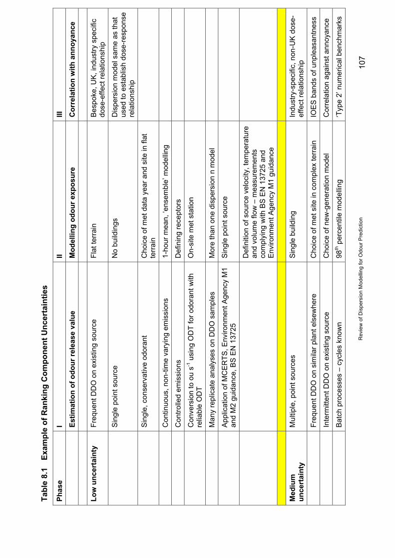
Rev
iew
of D
ispe
rsio
n M
odel
ling
for O
dour
Pre
dict
ion
107
Tabl
e 8.
1Ex
ampl
e of
Ran
king
Com
pone
nt U
ncer
tain
ties
Phas
eI
IIIII
Estim
atio
n of
odo
ur re
leas
e va
lue
Mod
ellin
g od
our e
xpos
ure
Cor
rela
tion
with
ann
oyan
ce
Low
unc
erta
inty
Freq
uent
DD
O o
n ex
istin
g so
urce
Flat
terr
ain
Bes
poke
, UK
, ind
ustry
spe
cific
dose
-effe
ct re
latio
nshi
p
Sin
gle
poin
t sou
rce
No
build
ings
Dis
pers
ion
mod
el s
ame
as th
atus
ed to
est
ablis
h do
se-r
espo
nse
rela
tions
hip
Sin
gle,
con
serv
ativ
e od
oran
tC
hoic
e of
met
dat
a ye
ar a
nd s
ite in
flat
terr
ain
Con
tinuo
us, n
on-ti
me
vary
ing
emis
sion
s1-
hour
mea
n, ‘e
nsem
ble’
mod
ellin
g
Con
trolle
d em
issi
ons
Def
inin
g re
cept
ors
Con
vers
ion
to o
u s-1
usi
ng O
DT
for o
dora
nt w
ithre
liabl
e O
DT
On-
site
met
sta
tion
Man
y re
plic
ate
anal
yses
on
DD
O s
ampl
esM
ore
than
one
dis
pers
ion
n m
odel
App
licat
ion
of M
CE
RTS
, Env
ironm
ent A
genc
y M
1an
d M
2 gu
idan
ce, B
S E
N 1
3725
Sin
gle
poin
t sou
rce
Def
initi
on o
f sou
rce
velo
city
, tem
pera
ture
and
volu
me
flow
– m
easu
rem
ents
com
plyi
ng w
ith B
S E
N 1
3725
and
Env
ironm
ent A
genc
y M
1 gu
idan
ce
Med
ium
unce
rtai
nty
Mul
tiple
, poi
nt s
ourc
esS
ingl
e bu
ildin
gIn
dust
ry-s
peci
fic, n
on-U
K d
ose-
effe
ct re
latio
nshi
p
Freq
uent
DD
O o
n si
mila
r pla
nt e
lsew
here
Cho
ice
of m
et s
ite in
com
plex
terr
ain
IOE
S b
ands
of u
nple
asan
tnes
s
Inte
rmitt
ent D
DO
on
exis
ting
sour
ceC
hoic
e of
new
-gen
erat
ion
mod
elC
orre
latio
n ag
ains
t ann
oyan
ce
Bat
ch p
roce
sses
– c
ycle
s kn
own
98th p
erce
ntile
mod
ellin
g‘T
ype
2’ n
umer
ical
ben
chm
arks

Rev
iew
of D
ispe
rsio
n M
odel
ling
for O
dour
Pre
dict
ion
108
Sur
roga
te w
ell c
orre
late
d w
ith to
tal o
dour
Mul
tiple
poi
nt s
ourc
esTo
lera
nce
fact
ors
depe
ndin
g on
rece
ivin
g po
pula
tion
Few
repl
icat
e an
alys
es o
n D
DO
sam
ples
Coa
stal
effe
cts
Hig
h U
ncer
tain
tyFu
gitiv
e/di
ffuse
sou
rces
Com
plex
terr
ain
Dut
ch li
vest
ock
dose
-effe
ctre
latio
nshi
p
Are
a/vo
lum
e so
urce
sM
ultip
le b
uild
ings
Cor
rela
tion
agai
nst c
ompl
aint
s
Con
vers
ion
to o
u s-1
usi
ng O
DT
for o
dora
nt w
ithun
relia
ble
OD
TU
se o
f flu
ctua
tions
mod
ellin
gB
ackg
roun
d od
ours
Non
-con
serv
ativ
e od
oran
t/mix
ture
of o
dora
nts
Pea
k-to
-mea
n ra
tios
FID
OL
fact
ors
Tim
e-va
ryin
g em
issi
ons
99th -
100th
per
cent
ile m
odel
ling
‘Typ
e 1’
det
erm
inis
tic a
ppro
ach
Est
imat
ion
of o
dour
rele
ase
rate
usi
ng O
dour
Pot
entia
lA
rea/
near
-gro
und/
volu
me
sour
ces
Dis
pers
ion
mod
el d
iffer
ent t
oth
at u
sed
to e
stab
lish
dose
-re
spon
se re
latio
nshi
p
Pub
lishe
d E
mis
sion
Fac
tors
Hor
izon
tal r
elea
ses
Sou
rce
stre
ngth
dep
ende
nt o
n am
bien
tw
eath
er c
ondi
tions
/unc
ontro
lled
Cap
ped/
obst
ruct
ed re
leas
es
Mas
s ba
lanc
e ca
lcul
atio
nsS
ingl
e m
odel
Sur
roga
te p
oorly
cor
rela
ted
with
tota
l odo
urP
lum
e de
posi
tion,
was
hout
, che
mis
try
Aba
tem
ent p
lant
effi
cien
cy
Review of Dispersion Modelling for Odour Prediction 109
9 Recommendations
9.1 Determination of Source Strength
The use of a specific surrogate compound, followed by conversion to ouE m-3
using the Odour Detection Threshold (ODT), adds a layer of uncertainty. Theuncertainty in this conversion can be the dominant factor affecting theuncertainty of the release value that goes into the atmospheric dispersionmodel. It is recommended that the Environment Agency makes clear in itsguidance that it prefers odour release rates to be obtained directly from ouE m-3,and that it does not favour the use of a specific surrogate compound followed byconversion to ouE m-3 using the ODT.
For the estimation of the source emission rate, the obvious route for minimising‘human error’ would be to ensure all such odour measurements for regulatorypurposes are carried out under the MCERTS scheme.
9.2 Odour emission factorsThere is a need for an openly available, centralised database for odour emissionfactors, or at least figures on which uncertainty has been quantified. Currently,commercial organisations have compiled their own databases, which are notwidely available. Sparse information is available from disparate sources (e.g.conference publications for agricultural odours, or the waste water industry). Acentralised database should be regularly reviewed, upgraded and updated,operator/industrial users of the database should be invited to verify the emissionfactors.
9.3 Dispersion modelling
UK dose-effect relationships should be established using the latest versions ofADMS and AERMOD PRIME, in an effort to move away from benchmarkswhich were established using dispersion models which are no longer the mostup to date with respect to treatment of boundary layer parameters, and whichapplicants are unlikely to use as part of the odour impact assessment. Suchmodelling will provide a more robust underpinning for the Draft H4 benchmarks,in their current form or if/once they are revised on the basis of modelling usingmore recent models and versions thereof.A model is only ‘better’ than another for predicting annoyance level if it hasbeen demonstrated to provide a better fit to the regression line in actual dose-effect data for the local situation. In the absence of any robust UK dose-effectsurvey, model choice based on best-fit of this regression is not possible.
The results of different, new-generation models can vary by a factor of 8, for thecalculation of high percentiles. Therefore, it is recommended that more than onedispersion model be used for all assessments. This is particularly important
Review of Dispersion Modelling for Odour Prediction110
when buildings and/or area sources are included in the modelling Examinationof the range of results would provide a sensitivity analysis of the modelalgorithms, and provide greater confidence in any regulatory decision.
9.4 Model inter-comparison
Discussions with AQMAU have led Bureau Veritas to understand that theEnvironment Agency has carried out tests on ADMS-3.3, and comparisonagainst ADMS3.2. The findings of this study, when available, could prove usefulfor the review of uncertainties in dispersion modelling. In particular, there isconcern over the way in which ADMS3.2 and earlier versions calculated thehigh percentiles, which are relevant for odour assessments.
9.5 Dutch livestock modelling
The original LTDF dispersion modelling data which underpinned setting of theodour standard in the Netherlands has not been available or traceable by UKinterested parties (Bull 2004). This continues to be the case.
For the purposes of assessing the validity of the Draft H4 Indicative OdourExposure Standards, it is important to identify how typical LTDF is of other ‘old-generation’ models. It would be particularly useful to be able to identify anysimilarity between LTDF and ISC in their respective predictions of the 98th
percentile concentrations. ISC has been subject to most inter-comparisonagainst ‘new-generation’ models. Technical details on LTDF could not beobtained during the course of Project 3.
9.6 FluctuationsDose-effect studies using dispersion models with facilities for estimatingfluctuations could be encouraged. Fluctuation modelling provides an opportunityto progress the understanding and development of ‘Type 1‘ numericalbenchmarks. This would add to the field validation for fluctuations models. Theextent of field validation available for fluctuation modelling, even forconservative pollutants without the complications of odorant FIDOLcharacteristics, is currently very low. Therefore, it is not yet advisable to setnumerical benchmarks based on modelling using fluctuations or peak-to-meanratios.
Dispersion models are currently in practical use only for predicting ensemblemean (typically hourly mean) concentrations. Fluctuation modelling is not yetadequately validated. As long as this remains the case, the ‘Type 2’ approachfor odour assessment set out in Draft H4 (hourly mean modelling comparedagainst an empirical benchmark) must remain the only feasible option.
Review of Dispersion Modelling for Odour Prediction 111
9.7 UK epidemiological dose-effect survey
The only realistic way of estimating the actual level of annoyance in a particularcommunity resulting from exposure is by carrying out dose-effect studies locally.Such a study links the exposure (determined by mathematical modelling ofemissions from the installation) to the level of annoyance (which is determinedby a standardised questionnaire). The relationship between calculated odourexposure and percentage of people annoyed as measured by survey has beenexperimentally confirmed in the Netherlands, but not in the UK. UK-specificdose-effect studies should be a priority area for research, and have alreadybeen identified in such in Environment Agency Report P4-095/TR (EnvironmentAgency 2002b). An application for an existing process could be obliged to carryout a dose-effect survey, to assist in establishing a database. In theNetherlands, the annoyance caused by odour is investigated by systematicyear-on-year community surveys (which disguise the purpose to avoid bias).Consideration should be given to establishing surveys or at least representativepilot studies of this kind in the UK
Draft H4 allows PPC applicants to derive industry-specific dose-responserelationships between annoyance and modelled 98th percentile odourconcentration, as an alternative to using the Draft H4 Indicative Odour ExposureStandards. As yet, the Environment Agency has received no application whichhas used such a bespoke dose-response relationship. It is likely that a stricterobligation may need to be put on certain operators to establish bespokerelationships for their industry sector.
It is possible that some dose-response studies will be performed around wastemanagement facilities as part of a study into defining loss of amenity throughodour carried out as part of Defra’s waste research R&D programme.
9.8 Is detailed modelling appropriate?There is a need to recognise that the uncertainties associated with modellingsome types of odorous release (e.g. diffuse/fugitive area sources, non-verticalvents) are very large. In such cases, the use of dispersion modelling as anassessment tool may not be an appropriate use of resources.It is important that dispersion modelling is not misused. Consideration could begiven to incorporating the following guidance into Draft H4.
• Only use odour dispersion modelling for new activities where thepredominant odour effect is due to normal process discharges that arecontinuous or semi-continuous and reliable odour emission rates areavailable.
• Do not use odour dispersion modelling to try to prove the absence of anadverse effect when community data can be collected, or are available todemonstrate the current level of effect.
Review of Dispersion Modelling for Odour Prediction112
• Do not use dynamic dilution olfactometry (DDO) measurement anddispersion modelling to investigate potential acute effects of odourdischarge.
• Give careful consideration to the validity of modelling low or area sourcesin the presence of buildings.
• Give careful consideration to the validity of modelling non-vertical orobstructed releases.
• Give careful consideration to the validity of modelling in the presence ofterrain.
9.9 Information required by Draft H4Draft H4 states that the level of detail supplied should be in keeping with the riskof causing odour-related annoyance at sensitive receptors. More details thanthose currently stipulated could be requested in the application for an PPCpermit. This could include the following, to help to indicate the potentialuncertainty:
• Dispersion modelling using more than one model;• Applicant to assign range of uncertainty to the values of odour
emission rate;• Applicant to fully justify lack of actual source strength
measurement for existing process, if applicable. A balance needsto be struck between cost/effort versus benefit/risk;
• For existing process with an existing odour problem, applicant topresent findings of a dose-effect survey.
These requirements would need to be set out in the PPC Sector GuidanceNotes. However, odour-related issues can be very installation-specific, and theoperator may wish to justify why some of this information is not appropriate for aparticular site.
ADMLC has provided detailed guidance on best practice for dispersionmodelling. Most of the guidelines are applicable to odour modelling. It would beuseful if these guidelines were incorporated into Draft H4, giving a clearer steertowards the required level of transparency and rigour in odour assessments.Also, some uniformity in the way that model sensitivity and uncertainty areexpressed could be imposed.
9.10 A Checklist for Inspectors
Although beyond the scope of his study, the findings of this Project 3 report, andin particular the information contained in Figures 4.1, 4.2, 5.1,5.2, 6.1 and 6.2,and Table 8.1, could be used to construct a checklist for Inspectors, to assistwith the review of an odour assessment.
Review of Dispersion Modelling for Odour Prediction 113
Abbreviations and acronymsADMLC Atmospheric Dispersion Modelling Liaison Committee
ADMS Atmospheric Dispersion Modelling System
AERMOD United States Environmental Protection Agency RegulatoryDispersion Model
AQMAU Air Quality Modelling and Assessment Unit
AQS Air Quality Strategy
BAT Best Available Technique
BS British Standard
BV Bureau Veritas
CEN Comité Européen de Normalisation/European Committeefor Standardisation
CEM continuous emissions monitor
CERC Cambridge Environmental Research Consultants
CFD computational fluid dynamics
CIWEM Chartered Institution of Water and EnvironmentalManagement
CRM certified reference material
DDO dynamic dilution olfactometry
Defra Department for Environment, Food and Rural Affairs
Draft H4 ‘Horizontal guidance for odour’, Environment Agency IPPCH4 Integrated Pollution Prevention and Control, October2002
EFD Emission Factors Database
EIA Environmental Impact Assessment
ELV Emission Limit Value
EPA Environmental Protection Act or Environmental ProtectionAgency
Review of Dispersion Modelling for Odour Prediction114
EROM European Reference Odour Mass
FIDOL frequency, intensity, duration, offensiveness, location
FPD flame photometric detector
GIS Geographical Information Systems
IOES Indicative Odour Exposure Standard
IPC Integrated Pollution and Control
ISC/ISCST Industrial Source Complex/Industrial Source ComplexShort Term (dispersion model)
ISO International Organisation for Standardisation
LTDF Lange Termijn Frequentie Distributie (Dutch regulatorymodel)
MCERTS Monitoring Certification Scheme
NRPB National Radiological Protection Board
OCI odour concentration–intensity (relationship)
ODT odour detection threshold
OP Odour Potential
ouE m-3 European odour units per cubic metre of air
NH3 ammonia
PDF probability distribution function
PPC Pollution Prevention and Control
ppm parts per million
PT proficiency testing
QA/QC quality assurance/quality control
R&D research and development
RMetS Royal Meteorological Society
STA Source Testing Association

Review of Dispersion Modelling for Odour Prediction 115
STOP Sewage Treatment Odour Prediction model
U uncertainty
UKWIR UK Water Industry Research
UV ultraviolet
VDI Verein Deutscher Ingenieure (standards)
VOC volatile organic compound
WASP Workplace Analysis Scheme for Proficiency
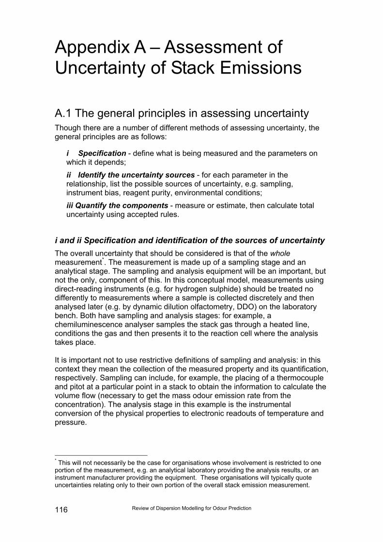
Review of Dispersion Modelling for Odour Prediction116
Appendix A – Assessment ofUncertainty of Stack Emissions
A.1 The general principles in assessing uncertaintyThough there are a number of different methods of assessing uncertainty, thegeneral principles are as follows:
i Specification - define what is being measured and the parameters onwhich it depends;ii Identify the uncertainty sources - for each parameter in therelationship, list the possible sources of uncertainty, e.g. sampling,instrument bias, reagent purity, environmental conditions;iii Quantify the components - measure or estimate, then calculate totaluncertainty using accepted rules.
i and ii Specification and identification of the sources of uncertaintyThe overall uncertainty that should be considered is that of the wholemeasurement*. The measurement is made up of a sampling stage and ananalytical stage. The sampling and analysis equipment will be an important, butnot the only, component of this. In this conceptual model, measurements usingdirect-reading instruments (e.g. for hydrogen sulphide) should be treated nodifferently to measurements where a sample is collected discretely and thenanalysed later (e.g. by dynamic dilution olfactometry, DDO) on the laboratorybench. Both have sampling and analysis stages: for example, achemiluminescence analyser samples the stack gas through a heated line,conditions the gas and then presents it to the reaction cell where the analysistakes place.
It is important not to use restrictive definitions of sampling and analysis: in thiscontext they mean the collection of the measured property and its quantification,respectively. Sampling can include, for example, the placing of a thermocoupleand pitot at a particular point in a stack to obtain the information to calculate thevolume flow (necessary to get the mass odour emission rate from theconcentration). The analysis stage in this example is the instrumentalconversion of the physical properties to electronic readouts of temperature andpressure.
* This will not necessarily be the case for organisations whose involvement is restricted to oneportion of the measurement, e.g. an analytical laboratory providing the analysis results, or aninstrument manufacturer providing the equipment. These organisations will typically quoteuncertainties relating only to their own portion of the overall stack emission measurement.
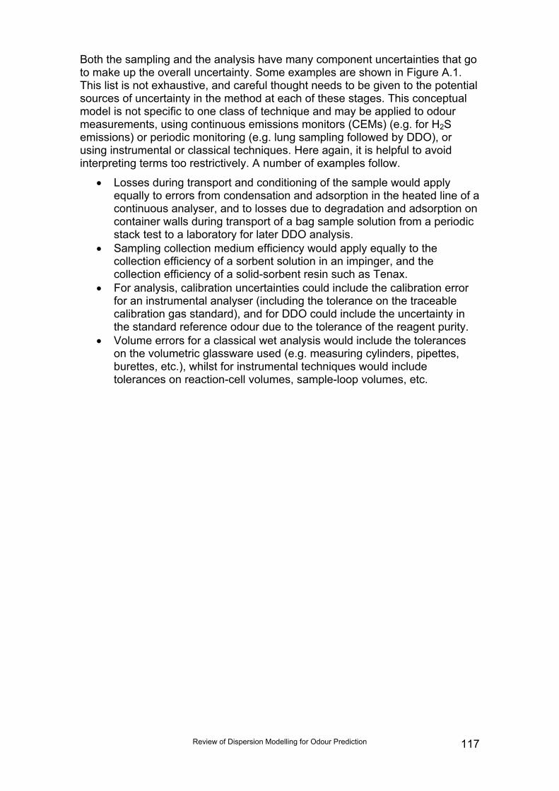
Review of Dispersion Modelling for Odour Prediction 117
Both the sampling and the analysis have many component uncertainties that goto make up the overall uncertainty. Some examples are shown in Figure A.1.This list is not exhaustive, and careful thought needs to be given to the potentialsources of uncertainty in the method at each of these stages. This conceptualmodel is not specific to one class of technique and may be applied to odourmeasurements, using continuous emissions monitors (CEMs) (e.g. for H2Semissions) or periodic monitoring (e.g. lung sampling followed by DDO), orusing instrumental or classical techniques. Here again, it is helpful to avoidinterpreting terms too restrictively. A number of examples follow.
• Losses during transport and conditioning of the sample would applyequally to errors from condensation and adsorption in the heated line of acontinuous analyser, and to losses due to degradation and adsorption oncontainer walls during transport of a bag sample solution from a periodicstack test to a laboratory for later DDO analysis.
• Sampling collection medium efficiency would apply equally to thecollection efficiency of a sorbent solution in an impinger, and thecollection efficiency of a solid-sorbent resin such as Tenax.
• For analysis, calibration uncertainties could include the calibration errorfor an instrumental analyser (including the tolerance on the traceablecalibration gas standard), and for DDO could include the uncertainty inthe standard reference odour due to the tolerance of the reagent purity.
• Volume errors for a classical wet analysis would include the toleranceson the volumetric glassware used (e.g. measuring cylinders, pipettes,burettes, etc.), whilst for instrumental techniques would includetolerances on reaction-cell volumes, sample-loop volumes, etc.
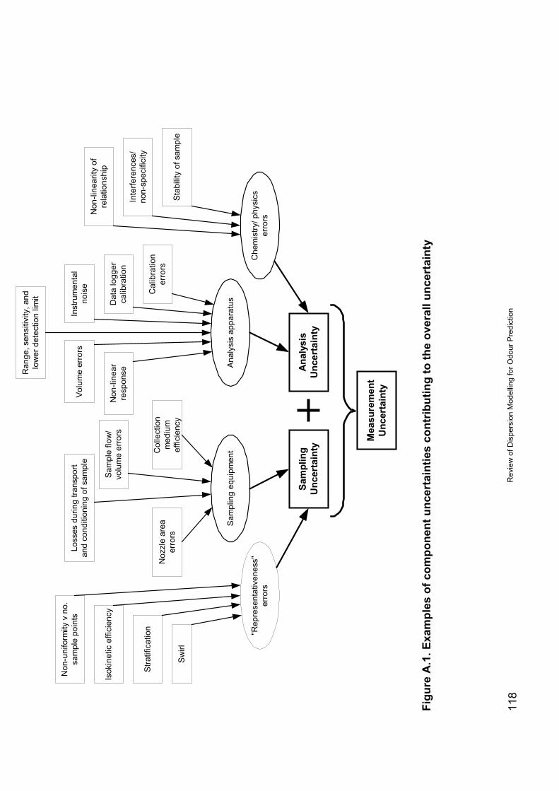
Rev
iew
of D
ispe
rsio
n M
odel
ling
for O
dour
Pre
dict
ion
118
Figu
re A
.1. E
xam
ples
of c
ompo
nent
unc
erta
intie
s co
ntrib
utin
g to
the
over
all u
ncer
tain
ty
"Rep
rese
ntat
iven
ess"
erro
rs
Sam
plin
g eq
uipm
ent
Anal
ysis
app
arat
us
Che
mis
try/ p
hysi
cser
rors
Sam
plin
gU
ncer
tain
tyA
naly
sis
Unc
erta
inty
Mea
sure
men
tU
ncer
tain
ty
Non
-uni
form
ity v
no.
sam
ple
poin
ts
Isok
inet
ic e
ffici
ency
Stra
tific
atio
n
Swirl
Loss
es d
urin
g tra
nspo
rtan
d co
nditi
onin
g of
sam
ple
Sam
ple
flow
/vo
lum
e er
rors
Col
lect
ion
med
ium
effic
ienc
y
Noz
zle
area
erro
rs
Ran
ge, s
ensi
tivity
, and
low
er d
etec
tion
limit
Non
-line
arre
spon
se
Inst
rum
enta
lno
ise
Dat
a lo
gger
calib
ratio
n
Cal
ibra
tion
erro
rs
Volu
me
erro
rs
Non
-line
arity
of
rela
tions
hip
Inte
rfere
nces
/no
n-sp
ecifi
city
Stab
ility
of s
ampl
e
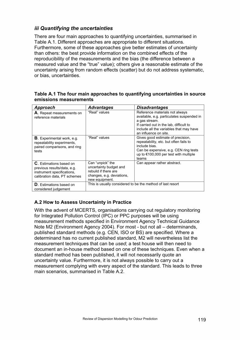
Review of Dispersion Modelling for Odour Prediction 119
iii Quantifying the uncertaintiesThere are four main approaches to quantifying uncertainties, summarised inTable A.1. Different approaches are appropriate to different situations.Furthermore, some of these approaches give better estimates of uncertaintythan others: the best provide information on the combined effects of thereproducibility of the measurements and the bias (the difference between ameasured value and the “true” value); others give a reasonable estimate of theuncertainty arising from random effects (scatter) but do not address systematic,or bias, uncertainties.
Table A.1 The four main approaches to quantifying uncertainties in sourceemissions measurementsApproach Advantages DisadvantagesA. Repeat measurements onreference materials
“Real” values Reference materials not alwaysavailable, e.g. particulates suspended ina gas stream.If carried out in the lab, difficult toinclude all the variables that may havean influence on site.
B. Experimental work, e.g.repeatability experiments,paired comparisons, and ringtests
“Real” values Gives good estimate of precision,repeatability, etc. but often fails toinclude bias.Can be expensive, e.g. CEN ring testsup to €100,000 per test with multipleteams
C. Estimations based onprevious results/data, e.g.instrument specifications,calibration data, PT schemes
Can “unpick” theuncertainty budget andrebuild if there arechanges, e.g. deviations,new equipment.
Can appear rather abstract.
D. Estimations based onconsidered judgement
This is usually considered to be the method of last resort
A.2 How to Assess Uncertainty in PracticeWith the advent of MCERTS, organisations carrying out regulatory monitoringfor Integrated Pollution Control (IPC) or PPC purposes will be usingmeasurement methods specified in Environment Agency Technical GuidanceNote M2 (Environment Agency 2004). For most - but not all – determinands,published standard methods (e.g. CEN, ISO or BS) are specified. Where adeterminand has no current published standard, M2 will nevertheless list themeasurement techniques that can be used; a test house will then need todocument an in-house method based on one of these techniques. Even when astandard method has been published, it will not necessarily quote anuncertainty value. Furthermore, it is not always possible to carry out ameasurement complying with every aspect of the standard. This leads to threemain scenarios, summarised in Table A.2.
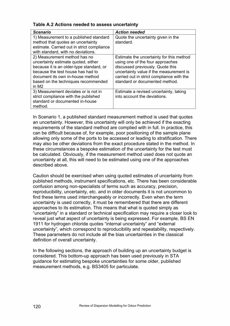
Review of Dispersion Modelling for Odour Prediction120
Table A.2 Actions needed to assess uncertaintyScenario Action needed1) Measurement to a published standardmethod that quotes an uncertaintyestimate. Carried out in strict compliancewith standard, with no deviations.
Quote the uncertainty given in thestandard.
2) Measurement method has nouncertainty estimate quoted, eitherbecause it is an older-type standard, orbecause the test house has had todocument its own in-house methodbased on the techniques recommendedin M2
Estimate the uncertainty for this methodusing one of the four approachesdiscussed previously. Quote thisuncertainty value if the measurement iscarried out in strict compliance with thestandard or documented method.
3) Measurement deviates or is not instrict compliance with the publishedstandard or documented in-housemethod.
Estimate a revised uncertainty, takinginto account the deviations.
In Scenario 1, a published standard measurement method is used that quotesan uncertainty. However, this uncertainty will only be achieved if the exactingrequirements of the standard method are complied with in full. In practice, thiscan be difficult because of, for example, poor positioning of the sample planeallowing only some of the ports to be accessed or leading to stratification. Theremay also be other deviations from the exact procedure stated in the method. Inthese circumstances a bespoke estimation of the uncertainty for the test mustbe calculated. Obviously, if the measurement method used does not quote anuncertainty at all, this will need to be estimated using one of the approachesdescribed above.
Caution should be exercised when using quoted estimates of uncertainty frompublished methods, instrument specifications, etc. There has been considerableconfusion among non-specialists of terms such as accuracy, precision,reproducibility, uncertainty, etc. and in older documents it is not uncommon tofind these terms used interchangeably or incorrectly. Even when the termuncertainty is used correctly, it must be remembered that there are differentapproaches to its estimation. This means that what is quoted simply as“uncertainty” in a standard or technical specification may require a closer look toreveal just what aspect of uncertainty is being expressed. For example, BS EN1911 for hydrogen chloride quotes “internal uncertainty” and “externaluncertainty”, which correspond to reproducibility and repeatability, respectively.These parameters do not include all the bias uncertainties in the classicaldefinition of overall uncertainty.
In the following sections, the approach of building up an uncertainty budget isconsidered. This bottom-up approach has been used previously in STAguidance for estimating bespoke uncertainties for some older, publishedmeasurement methods, e.g. BS3405 for particulate.

Review of Dispersion Modelling for Odour Prediction 121
A.3 The Uncertainty Budget Approach
OverviewAs with all the approaches, the general principles that apply are:
i. specification of the component parts of the measurement; ii. identify the sources of uncertainty for these components; and iii. quantify uncertainty components and combine them.
In the first stage, it is necessary to think about all the significant steps in themeasurement, including both sampling and analysis. The second stage involveslooking critically at these steps and listing the sources of uncertainty.
This may result in a large number of component uncertainties. Because thethird step involves quantifying these, it is useful to focus on a shortlist of thosemaking the most significant contributions. By convention, those componentsexpected to contribute less than a third of the largest need not be evaluated indetail.
Quantifying the component uncertaintiesThis is perhaps the most challenging step. Information on the magnitude of thecomponent uncertainties may often be found in the following sources.
• Published standards, especially the most modern ones – often limitspecifications are placed on some of the measurement components, e.g.sample volume must be measured to within ±x%, nozzle area must be within±y% of the nominal value;
• Manufacturers’ specifications – the technical specifications for an instrumentor piece of apparatus will often give valuable information on the componentuncertainties. For example, an infrared analyser spec may state thattemperature drift is ±x% between 0 and 50 ºC. A wet-chemistry examplewould be a 500 ml measuring cylinder used to measure the volume ofsorbent solution from the impingers. If the glassware conforms toBS604:1982, the graduations will be every 5 ml and the maximum permittederror in the graduations will be 5 ml. The error in the cylinder plus the error inreading will therefore be up to 7.5 ml.
• Calibration certificates – such data can be useful in a number of ways:calibration certificates, such as those provided for calibration of balances,may themselves quote the degree of uncertainty for the calibration. Once anumber of successive calibrations have been carried out, the drift can beestimated. In other applications, a tolerance is quoted. For example, acalibration gas may state a nominal concentration ± 5 %.
• QA/QC data – much of the data produced as part of a monitoringorganisations ongoing quality system can be used in the uncertainty budget.For instance, daily drift-checks on balances, daily checks on nozzlediameters and monthly checks on thermocouples and manometers mayprovide better estimates of their component uncertainties than simply takingas default values the limit specifications in the published standard. Similarly,the pre- and post-sampling span and zero checks that should be made on
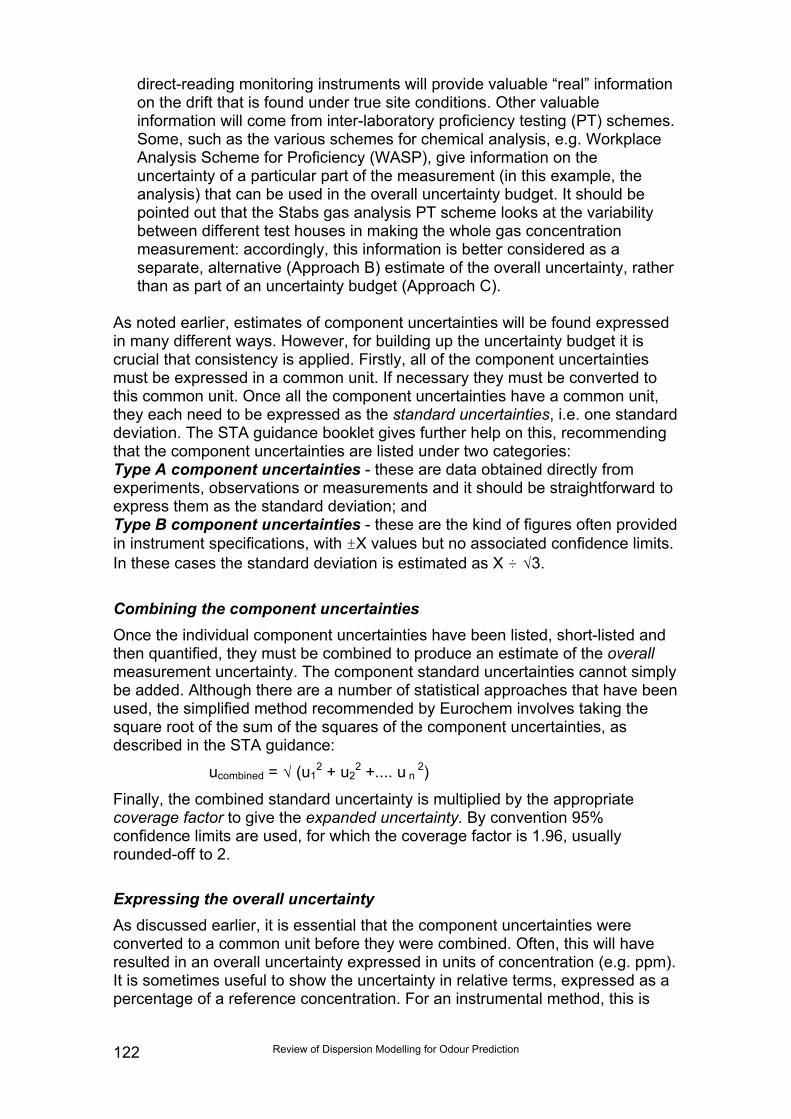
Review of Dispersion Modelling for Odour Prediction122
direct-reading monitoring instruments will provide valuable “real” informationon the drift that is found under true site conditions. Other valuableinformation will come from inter-laboratory proficiency testing (PT) schemes.Some, such as the various schemes for chemical analysis, e.g. WorkplaceAnalysis Scheme for Proficiency (WASP), give information on theuncertainty of a particular part of the measurement (in this example, theanalysis) that can be used in the overall uncertainty budget. It should bepointed out that the Stabs gas analysis PT scheme looks at the variabilitybetween different test houses in making the whole gas concentrationmeasurement: accordingly, this information is better considered as aseparate, alternative (Approach B) estimate of the overall uncertainty, ratherthan as part of an uncertainty budget (Approach C).
As noted earlier, estimates of component uncertainties will be found expressedin many different ways. However, for building up the uncertainty budget it iscrucial that consistency is applied. Firstly, all of the component uncertaintiesmust be expressed in a common unit. If necessary they must be converted tothis common unit. Once all the component uncertainties have a common unit,they each need to be expressed as the standard uncertainties, i.e. one standarddeviation. The STA guidance booklet gives further help on this, recommendingthat the component uncertainties are listed under two categories:Type A component uncertainties - these are data obtained directly fromexperiments, observations or measurements and it should be straightforward toexpress them as the standard deviation; andType B component uncertainties - these are the kind of figures often providedin instrument specifications, with ±X values but no associated confidence limits.In these cases the standard deviation is estimated as X ÷ √3.
Combining the component uncertaintiesOnce the individual component uncertainties have been listed, short-listed andthen quantified, they must be combined to produce an estimate of the overallmeasurement uncertainty. The component standard uncertainties cannot simplybe added. Although there are a number of statistical approaches that have beenused, the simplified method recommended by Eurochem involves taking thesquare root of the sum of the squares of the component uncertainties, asdescribed in the STA guidance:
ucombined = √ (u12 + u2
2 +.... u n 2)
Finally, the combined standard uncertainty is multiplied by the appropriatecoverage factor to give the expanded uncertainty. By convention 95%confidence limits are used, for which the coverage factor is 1.96, usuallyrounded-off to 2.
Expressing the overall uncertaintyAs discussed earlier, it is essential that the component uncertainties wereconverted to a common unit before they were combined. Often, this will haveresulted in an overall uncertainty expressed in units of concentration (e.g. ppm).It is sometimes useful to show the uncertainty in relative terms, expressed as apercentage of a reference concentration. For an instrumental method, this is

Review of Dispersion Modelling for Odour Prediction 123
often taken as that corresponding to 50% of the full scale reading. So if theinstrument is used typically on the 0-1000 ppm range, the overall uncertaintywill be expressed as a percentage of 500 ppm.
Overall uncertainty (%) = (U x 100) / Xref
It should be noted that if the mass emission is required to be calculated from theconcentration and the volume flow, then this will have a larger uncertainty.According to Hawksley et al (1977), the uncertainty is increased by a factor of√2, provided the stack gas flow has been measured according to BS3405.
The STA guidance booklet gives worked examples of uncertainty budgets forinstrumental methods, wet-chemistry methods and particulate monitoringmethods.
Review of Dispersion Modelling for Odour Prediction124
ReferencesADMLC 2001 ‘Options for the most appropriate meteorological data for use inshort-range dispersion modelling’ and ‘ Methods for undertaking uncertaintyanalyses’, ADMLC Annual Report 2000/2001.
ADMLC 2004 Guidelines for the Preparation of Dispersion ModellingAssessments for Compliance With Regulatory Requirements – An Update tothe 1995 Royal Meteorological Society Guidance. ADMLC/2004/1 V1 for publiccomment.
Auld, V., Hill, R. and Taylor, T.J. 2003 Uncertainty in Deriving DispersionParameters from Meteorological Data. Prepared for ADMLC by WestlakesScientific Consulting June 2003.
Best, P., Killip, C. and Brooke, A. 2004 Fragrance, fluctuations, facts or fantasy– the use, abuse and disuse of extreme statistics in odour evaluations. In:Enviro 2004 Conference seehttp://www.katestone.com.au/publications/ALL%20KATESTONE%20PAPERS%20pdf%20versions/Revised%20April%202004%20Enviro04_Best.pdf.
Bongers, M.E., Van Harreveld, A.P. and Jones, N. 2001 Recent developmentsin research supporting pig odour policy reviews in the Netherlands and Ireland.In: Proceedings of 1st IWA International Conference on Odour and VOCs,Measurement, Regulation and Control Techniques, University of New SouthWales, Sydney, March 2001, Ed. J. Jiang, pp 25–28. International WaterAssociation.
Both, R. and Koch, E. 2004 Odour regulation in Germany – an improved systemincluding odour intensity, hedonic tone and odour annoyance. In: Proceedingsof International Conference on Environmental Odour Management, Cologne,17–19 November 2004, pp 35–43. VDI-Berichte Nr. 1850. VDI Verlag GmbH.
Brady, J. (ed.) 2005 The IEMA Handbook, Environmental Management inOrganisations. James & James/Earthscan.
Bull, M.2003 Recent Experiences in Odour Assessment. Arup Environmental.
Bull, M. 2004 Implications of H4 odour standards and the practical uncertaintiesin their assessment. In: Proceedings of Conference Current Best PracticeTechniques for Odour Control, London, 23 March 2004. The Royal College ofPhysicians. Terence Dalton Ltd: Lavenham, Suffolk.
Bureau Veritas 2005 Uncertainty of Gas Flow rate Measurements using PitotStatic Tubes. Uncertainty Policy Document U14, February 2005.
Carruthers, D.J., McHugh, C.A., Dysters, S.J., Robins, A.G., Thomson, D.J.2001 Comments on EA Reports P353 & P362, Jan 2001. Available at:http://www.cerc.co.uk/software/pubs/comparison
Review of Dispersion Modelling for Odour Prediction 125
CERC 1998 Turbulence, Fluctuations and Averaging Times. CERC TechnicalNote, 22 December 1998.
Childs, P.S. and Hall, D.L. 2002 Use of dispersion modelling to define the heightof odour control stacks. Clean Air 32, Spring 2002.
Defra 2004 Local Authority Guidance on Odour from Sewage HandlingFacilities. Draft for public consultation, December 2004.
Defra 2006, Code of Practice on Odour Nuisance from Sewage TreatmentWorks, April 2006.
Department of Environmental Protection, Western Australia 2002 OdourMethodology Guideline. Available at http://portal.environment.wa.gov.au/pls/portal/url/ITEM/DFAF0FBAC29FACCFE03010AC6E052422.
DoE 2003 Report by the Inspector on a Public Inquiry into the Appeal byNorthumbrian Water Ltd for Additional Sewage Treatment Facilities on LandAdjacent to Spital Burn, Newbiggin by the Sea, Northumberland. DoEAPP/F2930/A/92/206240.
Dyster, S.J., Thomson, D.J., McHugh, C.A., Carruthers, D.J. 1999 Turbulentfluctuations and their use in estimating compliance with standards and in modelevaluation. Presented at 6th Harmonisation Conference, Rouen, 11-14 October1999.
Environment Agency 2002a Horizontal Guidance for Odour. TechnicalGuidance Note IPPC H4 (draft).
Environment Agency 2002b Assessment of Community Response to OdorousEmissions. Technical Report P4-095.
Environment Agency 2002c Best Available Techniques for Assessment andControl of Odour. Technical Report P4-079/TR/2.
Environment Agency 2002d Uncertainty and Sensitivity Analysis forEnvironmental Models. Technical Summary E2-S05/TS, August 2002. NERCcase studentship GT22/97/1/ES.
Environment Agency 2003 Odour Management at Intensive LivestockInstallations. IPPC SRC 6.02, Consultation draft, July 2003.
Environment Agency 2004 Technical Guidance Note (Monitoring) M2,Monitoring of Stack Emissions to Air. Environment Agency, Version 3, October2004.
Environment Agency 2006 Technical Guidance Document (Monitoring) M1,Sampling Requirements for Monitoring Stack Emissions to Air from IndustrialInstallationsVersion 4.
Environment Agency 2007a Review of Methods for Predicting and ModellingAgricultural and Livestock Emissions. Science Department Odour Cluster P4-120/2 Project 1.
Review of Dispersion Modelling for Odour Prediction126
Environment Agency 2007b Review of Odour Character and Thresholds –Literature Review. Science Department Odour Cluster P4-120/2 Project 2.
Environmental Protection Authority New South Wales 1995 Authorised OfficersManual. Available at http://www.epa.nsw.gov.au/mao/odourcontrol.htm
Eurochem 1995 Quantifying Uncertainty in Analytical Measurements. EurochemSecretariat, Teddington, UK.
Farrant, T. 1997 Practical Statistics for the Analytical Scientist – A Bench Guide.Royal Society of Chemistry, Cambridge.
Fisher, B. 2001 Treating predictions from more than one model. Presented atADMLC Workshop on Reliability of Atmospheric Dispersion Models, October2001, National Radiological Protection Board.
Fraser, F. 2004 Can STOP work (and can you make it stick)? CIWEM NationalConference 2004, RPS Consultants.
Fraser, F. 2005 Best Available Technique Odour from Animal Feeds Plant – ACase Study. Chartered Institute of Water and Environmental Management.
Freeman, T., Needham, C. and Schulz, T. 2000 Analysis of Options for OdourEvaluation for Industrial or Trade Processes. Report by CH2M BECA forAuckland Regional Council, New Zealand.
Garrison M. and Sherwell J. 1997 Evaluation of the AMS/EPA Regulatory Model(AERMOD) Complex Terrain Algorithms. Proceedings of the Air and WasteManagement Association’s 90th Annual Meeting and Exhibition, Toronto,Canada June 8-13 1997.
Gostelow, P. 2000 Emission rate estimation: art or sciences? In: 1stInternational Meeting on Odour Measurement and Modelling, May 2000,Cranfield University.
Habip, M. and Tripathi, A. 2004 Identification of an odour source from variousprobable sources in an industrial wastewater treatment plant. In: Proceedings ofInternational Conference on Environmental Odour Management, Cologne, 17–19 November 2004pp 453-462. VDI-Berichte Nr. 1850. VDI Verlag GmbH.
Hall, D.J. and Kukadia, V. 1994 Approaches to the calculation of dischargestack heights for odour control. Clean Air 24 (2), 75.
Hall, D.J., Spanton, A.M., 1999 Meteorological data and dispersion modelling.Envirobods Ltd. Stevenage.http://www.harmo.org/Intercomparison/MetMod2.pdf
Hall, D.J., Spanton, A.M., Bennett, M., Dunkerley, F., Griffiths, R.F., Fisher,B.E.A. and Timmis, R.J. 1999 Evaluation of new generation atmosphericdispersion models. In: Proceedings of 6th International Conference onHarmonisation within Dispersion Modelling for Regulatory Purposes, Rouen.International Journal of Environment and Pollution 2002 18(1) pp. 22-32.
Review of Dispersion Modelling for Odour Prediction 127
Hall, D.J. Spanton, A.M. Dunkerley, F. Bennett, M Griffiths, R.F. 2000a AReview of Dispersion Model Inter-Comparison Studies Using ISC, R91,AERMOD and ADMS. Environment Agency Technical Report P353.
Hall, D.J. Spanton, A.M. Bennett, M. Dunkerley, F. Griffiths, R.F. Fisher, B.E.A.Timmis, R.J. 2000b An Inter-Comparison of the AERMOD, ADMS and ISCDispersion Models for Regulatory Applications. Environment Agency TechnicalReport P362.
Hanna, S.R. Egan, B.A. Purdam, J. Wagler, J. 1999 Evaluation of the ADMS,AERMOD, and ISC3 dispersion Models with the Optex, Duke Forest, Kincaid,Indianapolis and Lovett Field data sets. CSI MS 5C3 George Mason Univ.Fairfax, VA 22030-4444 USA. http://www.cerc.co.uk/software/pubs/9%20-%20ADMS%20Aermod%20and%20ISC%20evaluation.pdf
Harvey, D.J. 1998 AERMOD and ADMS compared. Atmospheric DispersionModelling Ltd. Farnham, England.
Hawksley, P.G.W., Badzoich, S. and Blackett, J.H. 1977 Measurement of Solidsin Flue Gases. Institute of Fuel.
Hvitved-Jacobson, T. and Vollertsen, J. 2000 Formation modelling of odours insewer networks. In: 1st International Meeting on Odour Measurement andModelling, Cranfield University, May 2000.
ISO 1995 Guide to the Expression of Uncertainty in Analytical Measurement.ISO, Geneva.
Janicke, l., Janicke, U., Ahrens, D., Hartmann, U. and Muller, W.J. 2004Development of the odour dispersion model AUSTAL2000G in Germany. In:Proceedings of International Conference on Environmental Odour Management,Cologne, 17–19 November 2004. VDI-Berichte Nr. 1850. VDI Verlag GmbH.
Jones, J.A. Mayall, A. Cooper, P.J. 1995 Comparison of the ADMS and R91Atmospheric Dispersion Models. National Radiation Protection Board M572.
Lee, J. and Stewart, J.R. 1999 Omonos: A computer model for the dispersion ofodours in air. Clean Air 29. National Society for Clean Air and EnvironmentalProtection, Sept/Oct 1999, Brighton.
Lee, R.F., Goodman, A. and Heinerikson, A. (1999). Comparison betweenAERMOD and ISCST3 using data from three industrial plants. Paper No. 99-536. Air and Waste Management Association 90th Annual Meeting andExhibition in Saint Louis, Missouri, June 1999.
Lofstrom, P. 2004 Odour annoyance modelled as a single parameter. In:Proceedings of International Conference on Environmental Odour Management,Cologne, 17–19 November 2004, pp 529–532. VDI-Berichte Nr. 1850. VDIVerlag GmbH.
Lohmeyer, A. Czarnecki, S. Homans, W. J. Barth, S. Flassak, T. Frantz, H.2004a. GERDA - Tool for the Estimation of the Odour Emissions of 5 DifferentTypes of Plants. In: Proceedings of International Conference on Environmental
Review of Dispersion Modelling for Odour Prediction128
Odour Management, Cologne, 17-19 November 2004. VDI-Berichte Nr. 1850.VDI Verlag GmbH. pp 397-410
Lohmeyer, A. Baumuller, J. Flassak, T. Moldenhauer, A. Ruhling, A. 2004bAssessment and dispersion of odours in valley drainage flow. In: Proceedings ofInternational Conference on Environmental Odour Management, Cologne, 17-19 November 2004. VDI-Berichte Nr. 1850. VDI Verlag GmbH. pp169-178.
Longhurst, P. 2000 Exposure, perception and the application of odourmodelling. In: 1st International Meeting on Odour Measurement and Modelling,Cranfield University, May 2000.
Manning, K.S. and Jeavons, J.A. 1999 Odour control and planning arena.CIWEM/IAWQ Conference, September 1999, London.
Maul, P.R. Fisher, B.E.A. Bushell, S.D. 1996, Atmospheric Dispersion Modelsfor Integrated Pollution Control. Quanti Sci report no. IM4304-2, version 3.
McIntyre, A. 2000 Dispersion modelling of odours; tool or trap In: 1stInternational Meeting on Odour Measurement and Modelling, May 2000,Cranfield University.
Middleton, D.R. and Thomson, D.J. 2002 Uncertainties in Met Pre-Processingfor Dispersion Models. Met Office, Bracknell.
Miedema, H.M.E. 1992. Response Functions for Environmental Odour inResidential Areas. TNO report NIPG-publication No. 92.006. NetherlandsOrganisation of Applied Scientific Research (TNO), Leiden.
Miedema, H.M.E., Walpot, J.I. and Steunenberg, C.F. 2000 Exposure–annoyance relationships for odours from stationary sources. AtmosphericEnvironment 34, 2927–2936.
Ministry for the Environment New Zealand 2002 Review of Odour Managementin New Zealand: Technical Report. Air Quality Technical Report No. 24.Available at http://www.mfe.govt.nz/publications/air/odour-tr-aug02.html
Ministry for the Environment New Zealand 2003 Good Practice Guide forAssessing and Managing Odour in New Zealand. Air Air Quality Report 36,June 2003, Wellington, ISBN: 0-478-24090-2Available at http://www.mfe.govt.nz/publications/air/odour-guidelines-jun03/odour-guidelines-jun03.pdf
Minnesota Pollution Control Agency 2006 A Review of National andInternational Odour Policy, Odour Measurement Technology and PublicAdministration. Report SRF0034734 prepared by SRF Consulting Group Inc.,February 2006. Available at http://www.pca.state.mn.us/programs/odor.html.
Paine R.J., Lee R.F., Brode R., Wilson R.B., Cimorelli A.J., Perry S.G., WeilJ.C., Venkatram A., and Peters W.D. 1998 Model Evaluation Results forAERMOD. USEPA, RTP. NC 27711.
Review of Dispersion Modelling for Odour Prediction 129
Persson, P-E., Skog, S. and Hasenson, B. 1987 Complex odours in the vicinityof a petrochemical industrial complex. Journal of the Air Pollution ControlAssociation 37 (12), 1418–1420.
Peters, W.D. Paine, R.J. Lee, R.F. Wilson, R.B. Cimorelli, A.J. Perry, S.G. Weil,J.C. Venkatram, A. 1999 Comparison of Regulatory Design Concentrations-AERMOD versus ISCST3 and CTDMPLUS. USEPA. Available from:www.epa.gov/scram001
Pietarila, H. and Savunen, T. 2004 The waste management application of anodour dispersion model. In: Proceedings of International Conference onEnvironmental Odour Management, Cologne, 17–19 November 2004. VDI-Berichte Nr. 1850. VDI Verlag GmbH. pp 187-196
Pullen, J.C. 1998 Guidance on Assessing Measurement Uncertainty in StackEmissions Monitoring. Source Testing Association, Quality Guidance NoteQGN1.
Pullen, J.C. 2003 The application of uncertainty to stack monitoring. STATechnical Transfer Seminar, Uncertainty – The Way Forward, BretbyConference Centre, 20 February 2003.
Royal Meteorological Society 1995 Atmospheric Dispersion Modelling. RoyalMeteorological Society Policy Statement – May 1995.
Royal Society of Chemistry 2006 Uncertainties in Concentrations Estimatedfrom Calibration Experiments. Analytical Methods Committee, Technical BriefNo. 22. Royal Society of Chemistry, Cambridge. Available athttp://www.rsc.org/Membership/Networking/InterestGroups/Analytical/AMC/TechnicalBriefs.asp
Schauberger, G. and Piringer, M. 2004 Assessment of the odour concentrationin the near-field of small sources. In: Proceedings of International Conferenceon Environmental Odour Management, Cologne, 17–19 November 2004. VDI-Berichte Nr. 1850. VDI Verlag GmbH. pp343-352
Scottish Executive 2004 Consultation on a Draft Code of Practice onAssessment and Control of Odour Nuisance from Waste Water TreatmentWorks.
Shi, J.-P. and Ng, B. 2002 Risk-based pragmatic approach to address modeluncertainty. Environment Agency Air Quality Modelling and Assessment Unit,Model Uncertainty Workshop, October 2002, Cardiff, NSCA.
Sidle, C., Tuckett-Jones, B., Ng, B. and Ping Shi, J. 2004 Model inter-comparison between ADMS3.1, AERMOD and AERMOD PRIME. In: 9thInternational Conference on Harmonisation within Atmospheric DispersionModelling for Regulatory Purposes, Germany
Simms, K.L., Wilkinson, S. and Bethan, S. 1999 Odour Nuisance andDispersion Modelling: An Objective Approach to a Very Subjective Problem.Water Science and Technology, 41(6) 89-96.
Review of Dispersion Modelling for Odour Prediction130
Stuetz, R. and Frechen, F. (eds) 2001 Odours in Wastewater Treatment,Measurement, Modelling and Control. IWA Publishing.
UK WIR 2006 Best Practicable Means (BPM) – A Guidebook for Odour Controlat Wastewater Treatment Works (Draft). UK Water Industry Research.
US EPA 1992 Reference Guide to Odor Thresholds for Hazardous AirPollutants Listed in the Clean Air Act Amendments of 1990. United StatesEnvironmental Protection Agency, Office of Air Quality Planning and Standards,North Carolina.
US EPA 1995 Users’ Guide for the Industrial Source Complex (ISC3)Dispersion Models. US Environmental Protection Agency. EPA-454/B-95-003aand 003b.
US EPA 1999 Comparison of Regulatory Design Concentrations: AERMODversus ISCST3 and CTDMPLUS. US Environmental Protection Agency. EPA-454/R-03-002.
Van Harreveld A P and Dönszelmann C E P, 1994, Odour Nuisance: policyoptions and regulatory approach, Chartered Institute of Environmental Health,Welsh Council Weekend Course.
Van Harreveld, A.P. 2001 From odorant formation to odour nuisance: newdefinitions for discussing a complex process. Water Science and Technology 44(9), 9–15.
Van Harreveld A.P. 2004 How Much Odour is Annoying? In: Proceedings ofConference Current Best Practice Techniques for Odour Control, London,March 2004.
VDI 1997 Effects and Assessment of Odours – Psychometric Assessment ofOdour Annoyance Questionnaires. VDI 3883: Part 1. Verein DeutscherIngenieure, Dusseldorf. Available from Beuth Verlag GmbH.
VROM 1984 Lucht indicatief meerjaren programma lucht 1985–1989 (IndicativeLong-term Programme for Air Quality, 1985-1989). Ministry VROM, The Hague,Netherlands.
Werkgroep Verspreiding Luchtverontreiniging 1983 Frequentieverdelingen vanluchtverontreinigings-concentraties. Staatuitgeverij, Den Haag.
Wilson, D.J1995 . Concentration Fluctuations and Averaging Time in VapourClouds. Center for Chemical Process Safety. ISBN: 0-8169-0679-3.
Witherspoon J.R., Sidhu A., Castleberry J., Coleman L., Reynolds K., Card T.,Daigger G.T. 2000 Odour emission estimates and control strategies usingmodels and sampling for East Bay Municipal Utility District's collection sewagesystem and wastewater treatment plant. Water Science and Technology, 41 (6):65-71.
Woodfield, M. and Hall, D. (eds) 1994 Odour Measurement and Control – AnUpdate. AEA Technology for Department of the Environment.

Review of Dispersion Modelling for Odour Prediction 131
WRc 1998 Report UC 3110.
Yang, G. and Hobson, J. 1998 Validation of the wastewater treatment odourproduction (STOP) model. In Proceedings of the 2nd CIWEM NationalConference on Odour Control in Wastewater Treatment. London, 30th April1998.
Yang, G. and Hobson, J. 2000 Odour nuisance – advantages anddisadvantages of a quantitative approach. Journal of Water Science andTechnology 41 (6), 97–106.

We are The Environment Agency. It's our job to look afteryour environment and make it a better place – for you, andfor future generations.
Your environment is the air you breathe, the water you drinkand the ground you walk on. Working with business,Government and society as a whole, we are making yourenvironment cleaner and healthier.
The Environment Agency. Out there, making yourenvironment a better place.
Published by:
Environment AgencyRio HouseWaterside Drive, Aztec WestAlmondsbury, Bristol BS32 4UDTel: 0870 8506506Email: [email protected]
© Environment Agency
All rights reserved. This document may be reproduced withprior permission of the Environment Agency.


![Panasonic...Durian odour 6 Natural reduction 60tmin.] Sweat odour Nonanoic acid Natural reduction 120[min.] Garbage odour Methylmercaptan Natural reduction 601minJ Scalp odour Panasonic](https://img.pdfslide.us/doc/110x75/60d72199474aa2073d394000/panasonic-durian-odour-6-natural-reduction-60tmin-sweat-odour-nonanoic-acid.jpg)