Review of Basic Statistical Concepts Notes/Covariance.pdf · Review of Basic Statistical Concepts James H. Steiger Department of Psychology and Human Development Vanderbilt University

Review of Basic Statistical Concepts

James H. Steiger

Department of Psychology and Human DevelopmentVanderbilt University

James H. Steiger (Vanderbilt University) Review of Basic Statistical Concepts 1 / 87

Review of Basic Statistical Concepts1 Introduction

2 The Mean and the Expected Value

3 Listwise Operations and Linear Transformations in R

4 Deviation Scores, Variance, and Standard Deviation

5 Z -Scores

6 Covariance and Correlation

7 Covariance

The Concept of Covariance

Computing Covariance

Limitations of Covariance

8 The (Pearson) Correlation Coefficient

Definition

Computing

Interpretation

9 Some Other Correlation Coefficients

Introduction

10 Population Variance, Covariance and Correlation

11 Laws of Linear Combination

12 Significance Test for the Correlation Coefficient


Introduction

Introduction

In this module, we will quickly review key statistical concepts and their algebraicproperties.These concepts are taken for granted (more or less) in all graduate level discussions ofregression analysis.There are extensive review chapters available to help you gain/recover familiarity with theconcepts.


The Mean and the Expected Value

The Mean

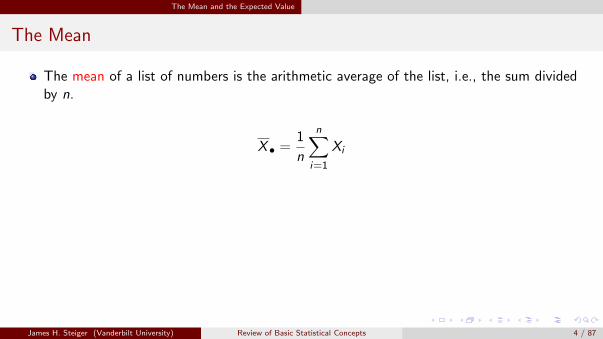
The mean of a list of numbers is the arithmetic average of the list, i.e., the sum dividedby n.

X • =1

n

n∑i=1

Xi



The Expected Value

The expected value of a random variable is the long run arithmetic average of the valuestaken on by the random variable.The expected value of a random variable X is denoted E (X ), and is also often simplyreferred to as the mean of the random variable X .



Algebraic Properties of Linear Transformation

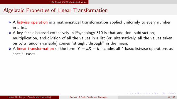
A listwise operation is a mathematical transformation applied uniformly to every numberin a list.A key fact discussed extensively in Psychology 310 is that addition, subtraction,multiplication, and division of all the values in a list (or, alternatively, all the values takenon by a random variable) comes “straight through” in the mean.A linear transformation of the form Y = aX + b includes all 4 basic listwise operations asspecial cases.



Algebraic Properties of Linear TransformationTheorem (Mean of a Linear Transform)

Suppose Y and X are random variables, and Y = aX + b for constants a and b. Then

E (Y ) = aE (X ) + b

If Y and X are lists of numbers and Yi = aXi + b, then a similar rule holds, i.e.,

Y • = aX • + b



Algebraic Properties of Linear TransformationExample (Listwise Transformation and the Sample Mean)

Suppose you have a list of numbers X with a mean of 5.

If you multiply all the X values by 2 and then add 3 to all those values, you have transformedX into a new variable Y by the listwise operation Y = 2X + 3.

In that case, the means of Y and X will be related by the same formula, i.e.,Y • = 2X • + 3 = 2(5) + 3 = 13.



Algebraic Properties of Linear TransformationExample (Listwise Transformation and the Population Mean)

Suppose you have a random variable X with an expected value of E (X ) = 10. Define therandom variable Y = 2X − 4. Then E (Y ) = 2E (X )− 4 = 20− 4 = 16.


Listwise Operations and Linear Transformations in R

Elementary Listwise Operations

Getting a short list of data into R is straightforward with an assignment statement.Here we create an X list with the integer values 1 through 5.

> X <- c(1,2,3,4,5)


Listwise Operations and Linear Transformations in R

Elementary Listwise Operations

Creating a new variable that is a linear transformation of the old one is easy:

> Y = 2*X + 5

> Y

[1] 7 9 11 13 15

And, the means of X and Y obey the linear transformation rule.

> mean(X)

[1] 3

> 2 * mean(X) + 5

[1] 11

> mean(Y)

[1] 11


Deviation Scores, Variance, and Standard Deviation


If we re-express a list of numbers in terms of where they are relative to their mean, wehave created deviation scores.Deviation scores are calculated as

dxi = Xi − X •

This is done easily in R as

> dx = X - mean(X)

> X

[1] 1 2 3 4 5

> dx

[1] -2 -1 0 1 2




If we want to measure how spread out a list of numbers is, we can look at the size ofdeviation scores.Bigger spread means bigger deviations around the mean.One might be tempted to use the average deviation score as a measure of spread, orvariability.But that won’t work.




Why Not?




A better idea is the average squared deviation.An even better idea, if you are estimating the average squared deviation in a largepopulation from the information in the sample, is to use the sample variance

S2X =

1

n − 1

n∑i=1

(Xi − X •)2

The sample standard deviation is simply the square root of the sample variance, i.e.,

SX =√

S2X




Computing the variance or standard deviation in R is very easy.

> var(X)

[1] 2.5

> sd(X)

[1] 1.581139



Linear Transformation Rules for Variances and Standard Deviations

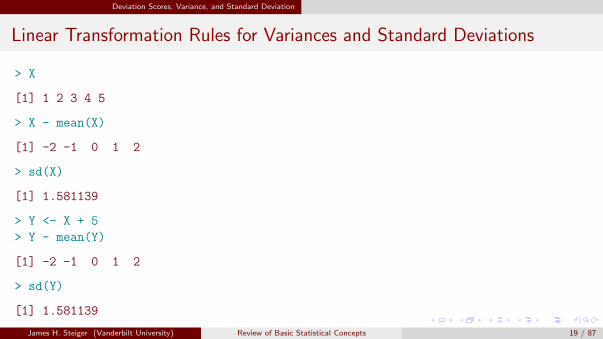
Multiplication or division comes straight through in the standard deviation if the multiplieris positive — otherwise the absolute value of the multiplier comes straight through.This makes sense if you recall that there is no such thing as a negative variance orstandard deviation!Additive constants have no effect on deviation scores, and so have no effect on thestandard deviation or variance.




INVESTIGATE! IN R!!




> X

[1] 1 2 3 4 5

> X - mean(X)

[1] -2 -1 0 1 2

> sd(X)

[1] 1.581139

> Y <- X + 5

> Y - mean(Y)

[1] -2 -1 0 1 2

> sd(Y)

[1] 1.581139




> Y <- 2*X + 5

> Y - mean(Y)

[1] -4 -2 0 2 4

> sd(Y)

[1] 3.162278

> var(Y)

[1] 10




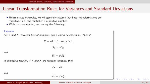
Unless stated otherwise, we will generally assume that linear transformations are“positive,” i.e., the multiplier is a positive number.With that assumption, we can say the following:

Theorem

Let Y and X represent lists of numbers, and a and b be constants. Then if

Y = aX + b and a > 0

SY = aSX

andS2Y = a2S2

X

In analogous fashion, if Y and X are random variables, then

σY = aσX

andσ2Y = a2σ2

X


Z -Scores

Z -Scores

In Psychology 310, we go into quite a bit of detail explaining how any list of numbers canbe thought of as having

1 Shape2 Metric, comprised of a mean and a standard deviation.


Z -Scores

Z -Scores

Shape, the pattern of relative interval sizes moving from left to right on the number line,is invariant under positive linear transformation.It can be thought of as the information in a list that “transcends scaling.”


Z -Scores

Z -Scores

Metric, the mean and standard deviation of the numbers, can be thought of as theinformation in a list that “reflects scaling.”In a lot of situations, “metric can be thought of as arbitrary.”


Z -Scores

Z -Scores

What does THAT mean??


Z -Scores

Z -Scores

If metric is arbitrary, do we need it??


Z -Scores

Z -Scores

Consider the Z score transformation, which transforms a list of X values as

Zi =Xi − X •

Sx

If we do this to a list of numbers, what will their mean and standard deviation (i.e., theirmetric) become?


Z -Scores

Z -Scores

Did your mind go blank??


Z -Scores

Z -Scores

If it did — a helpful strategy


Z -Scores

Z -Scores

Create a “random” list of numbers.Not too small, not too large, call it XNow, convert to Z scores and see what happens.

> X <- c(16.2,33,13.9,12.8,3.3)

> X

[1] 16.2 33.0 13.9 12.8 3.3

> Z <- (X - mean(X))/sd(X)

> mean(Z)

[1] 2.502339e-17

> sd(Z)

[1] 1


Z -Scores

Z -Scores

Now YOU try it.


Z -Scores

Z -Scores

It seems like, no matter what list of numbers we generate, the Z -transform converts themso that they have a mean of 0 (ignoring round-off error) and a standard deviation of 1.Now that we suspect we know the answer, we can perhaps be more confident as we setout to prove that, in fact, this suspicion is correct.


Z -Scores

Z -Scores

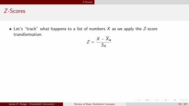
Let’s “track” what happens to a list of numbers X as we apply the Z -scoretransformation.

Z =X − X •

SX


Z -Scores

Z -Scores

We start in the numerator with the originalscores in X . What happens to the scores whenwe subtract X •?

Z =X − X •

SX

We recall from our linear transformation rules that subtracting the constant X • has no effecton the standard deviation of the scores, so the scores will still have a standard deviation of SX .However, subtracting X • reduces the mean of the scores by X •, so the mean has beenchanged to 0.

So at this stage of the transformation, we have scores with a mean of zero and a standarddeviation of SX .


Z -Scores

Z -Scores

Moving on to the next stage of thetransformation, we realize that dividing by SX

divides the standard deviation by SX , and sothe standard deviation becomes SX/SX = 1.

The mean is 0/SX = 0, and remainsunchanged.

We now see that what R demonstrated to usnumerically is mathematically inevitable.

Z =X − X •

SX


Z -Scores

Z -Scores

In an important sense, Z -scoring removes the metric from a list of numbers by renderingany list with the same, simple metric.We say that scores are in Z -score form if they have a mean of 0 and a standard deviationof 1.Once scores are in Z -score form, we can convert them into any other desired metric byjust mulitplying by the desired standard deviation, then adding the desired mean.


Covariance and Correlation

Bivariate Distributions and Covariance

Here’s a question that you’ve thought of informally, but probably have never been temptedto assess quantitatively: “What is the relationship between shoe size and height?”We’ll examine the question with a data set from an article by Constance McLaren in the2012 Journal of Statistics Education.



Bivariate Distributions and Covariance

The data file is available in several places on the course website. You may download thefile by right-clicking on it (it is next to the lecture slides).These data were gathered from a group of volunteer students in a business statisticscourse.If you place it in your working directory, you can then load it with the command

> all.heights <- read.csv("shoesize.csv")

Alternatively, you can download directly from a web repository with the command

> all.heights <- read.csv(

+ "http://www.statpower.net/R2101/shoesize.csv")



Bivariate Distributions and Scatterplots

We can isolate the male data from all the data with the following command:

> rm(X,Y) # remove old X,Y variables

> male.data <- all.heights[all.heights$Gender=="M",] #Select males

> attach(male.data)#Make Variables Available




Let’s draw a scatterplot:

> # Draw scatterplot

> plot(Size,Height,xlab="Shoe Size",ylab="Height in Inches")

8 10 12 14

6570

7580

Shoe Size

Hei

ght i

n In

ches




This scatterplot shows a clear connection between shoe size and height.Traditionally, the variable to be predicted (the dependent variable) is plotted on thevertical axis, while the variable to be predicted from (the independent variable) is plottedon the horizontal axis.Note that, because height is measured only to the nearest inch, and shoe size to thenearest half-size, a number of points overlap. The scaterplot indicates this by makingsome points darker than others.But how can we characterize this relationship accurately?We notice that shoe size and height vary together.A statistician might say they “covary.”This notion is operationalized in a statistic called covariance.




Let’s compute the average height and shoe size, and then draw lines of demarcation onthe scatterplot.

> mean(Height)

[1] 71.10552

> mean(Size)

[1] 11.28054




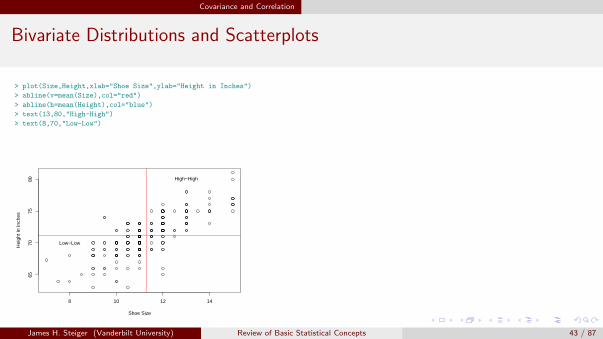
> plot(Size,Height,xlab="Shoe Size",ylab="Height in Inches")

> abline(v=mean(Size),col="red")

> abline(h=mean(Height),col="blue")

> text(13,80,"High-High")

> text(8,70,"Low-Low")

8 10 12 14

6570

7580

Shoe Size

Hei

ght i

n In

ches

High−High

Low−Low




The upper right (“High-High”) quadrant of the plot represents men whose heights andshoe sizes were both above average.The lower left (”Low-Low”) quadrant of the plot represents men whose heights and shoesizes were both below average.Notice that there are far more data points in these two quadrants than in the other two:This is because, when there is a direct (positive) relationship between two variables, thescores tend to be on the same sides of their respective means.On the other hand, when there is an inverse (negative) relationship between two variables,the scores tend to be on the opposite sides of their respective means.This fact is behind the statistic we call covariance.


Covariance The Concept of Covariance

CovarianceThe Concept

What is covariance?We convert each variable into deviation score form by subtracting the respective means.If scores tend to be on the same sides of their respective means, then

1 Positive deviations will tend to be matched with positive deviations, and2 Negative deviations will tend to be matched with negative deviations

To capture this trend, we sum the cross-product of the deviation scores, then divide byn − 1.So, essentially, the sample covariance between X and Y is an estimate of the averagecross-product of deviation scores in the population.


Covariance Computing Covariance

CovarianceComputations

The sample covariance of X and Y is defined as

sx ,y =1

n − 1

n∑i=1

(Xi − X •)(Yi − Y •) (1)

An alternate, more computationally convenient formula, is

sx ,y =1

n − 1

(n∑

i=1

XiYi −∑n

i=1 Xi∑n

i=1 Yi

n

)(2)

An important fact is that the variance of a variable is its covariance with itself, that is, ifwe substitute x for y in Equation 1, we obtain

s2x = sx ,x =

1

n − 1

n∑i=1

(Xi − X •)(Xi − X •) (3)




Computing the covariance between two variables “by hand” is tedious thoughstraightforward and, not surprisingly (because the variance of a variable is a covariance),follows much the same path as computation of a variance:

1 If the data are very simple, and especially if n is small and the sample mean a simplenumber, one can convert X and Y scores to deviation score form and use Equation 1.

2 More generally, one can compute∑

X ,∑

Y ,∑

XY , and n and use Equation 2.




Example (Computing Covariance)

Suppose you were interested in examining the relationship between cigarette smoking and lungcapacity. You asked 5 people how many cigarettes they smoke in an average day, and you thenmeasure their lung capacities, which are corrected for age, height, weight, and gender. Hereare the data:

Cigarettes Lung.Capacity

1 0 45

2 5 42

3 10 33

4 15 31

5 20 29

(. . . Continued on the next slide)





In this case, it is easy to compute the mean for both Cigarettes (X) and Lung Capacity (Y),i.e., X • = 10, Y • = 36, then convert to deviation scores and use Equation 1 as shown below:

X dX dXdY dY Y XY

1 0 -10 -90 9 45 0

2 5 -5 -30 6 42 210

3 10 0 0 -3 33 330

4 15 5 -25 -5 31 465

5 20 10 -70 -7 29 580

The sum of the dXdY column is −225, and we then compute the covariance as

sx ,y =1

n − 1

n∑i=1

dXidYi =−215

4= −53.75

(. . . Continued on the next slide)





Alternatively, one might compute∑

X = 50,∑

Y = 180,∑

XY = 1585, and n, and useEquation 2.

sx ,y =1

n − 1

(∑XY −

∑X∑

Y

n

)=

1

5− 1

(∑1585− 50× 180

5

)=

1

4

(∑1585− 9000

5

)=

1

4

(∑1585− 1800

)=

1

4(−215)

= −53.75

Of course, there is a much easier way, using R. (. . . Continued on the next slide)





Here is how to compute covariance using R’s cov command. In the case of really simpletextbook examples, you can copy the numbers right off the screen and enter them into R,using the following approach.

> Cigarettes <- c(0,5,10,15,20)

> Lung.Capacity <- c(45,42,33,31,29)

> cov(Cigarettes,Lung.Capacity)

[1] -53.75


Covariance Limitations of Covariance

CovarianceLimitations

Covariance is an extremely important concept in advanced statistics.Indeed, there is a statistical method called Analysis of Covariance Structures that is oneof the most widely used methodologies in Psychology and Education.However, in its ability to convey information about the nature of a relationship betweentwo variables, covariance is not particularly useful as a single descriptive statistic, and isnot discussed much in elementary textbooks.What is the problem with covariance?




We saw that the covariance between smoking and lung capacity in our tiny sample is−53.75.The problem is, this statistic is not invariant under a change of scale.As a measure on deviation scores, we know that adding or subtracting a constant fromevery X or every Y will not change the covariance between X and Y .However, multiplying every X or Y by a constant will multiply the covariance by thatconstant.It is easy to see that from the covariance formula, because if you multiply every raw scoreby a constant, you multiply the corresponding deviation score by that same constant.We can also verify that in R. Suppose we change the smoking measure to packs per dayinstead of cigarettes per day by dividing X by 20. This will divide the covariance by 20.




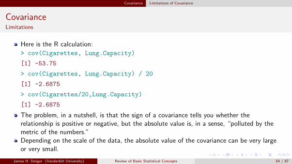
Here is the R calculation:

> cov(Cigarettes, Lung.Capacity)

[1] -53.75

> cov(Cigarettes, Lung.Capacity) / 20

[1] -2.6875

> cov(Cigarettes/20,Lung.Capacity)

[1] -2.6875

The problem, in a nutshell, is that the sign of a covariance tells you whether therelationship is positive or negative, but the absolute value is, in a sense, “polluted by themetric of the numbers.”Depending on the scale of the data, the absolute value of the covariance can be very largeor very small.




How can we fix this?


The (Pearson) Correlation Coefficient Definition

The (Pearson) Correlation CoefficientDefinition

To take the metric out of covariance, we compute it on the Z -scores instead of thedeviation scores. (Remember that Z -scores are also deviation scores, but they have thestandard deviation divided out.)The sample correlation coefficient rx ,y , sometimes called the Pearson correlation, butgenerally referred to as “the correlation” is simply the sum of cross-products of Z -scoresdivided by n − 1:

rx ,y =1

n − 1

n∑i=1

ZxiZyi (4)

The population correlation ρx ,y is the average cross-product of Z -scores for the twovariables.


The (Pearson) Correlation Coefficient Definition

The (Pearson) Correlation CoefficientDefinition

One may also define the correlation in terms of the covariance, i.e.,

rx ,y =sx ,ysxsy

(5)

Equation 5 shows us that we may think of a correlation coefficient as a covariance withthe standard deviations factored out.Alternatively, since we may turn the equation around and write

sx ,y = rx ,y sxsy (6)

we may think of a covariance as a correlation with the standard deviations put back in.


The (Pearson) Correlation Coefficient Computing

The (Pearson) Correlation CoefficientComputing the Correlation

Most textbooks give computational formulas for the correlation coefficient. This isprobably the most common version.

rx ,y =n∑

XY −∑

X∑

Y√[n∑

X 2 − (∑

X )2] [

n∑

Y 2 − (∑

Y )2] (7)

If we compute the quantities n,∑

X ,∑

Y ,∑

X 2,∑

Y 2,∑

XY , and substitute theminto Equation 7, we can calculate the correlation as shown on the next slide.




Example (Computing a Correlation)

rxy =(5)(1585)− (50)(180)√[

(5)(750)− 502] [

(5)(6680)− 1802]

=7925− 9000√

(3750− 2500)(33400− 32400)

=−1075√

(1250) (1000)

= −.9615

(Continued on the next slide . . . )




Example (Computing a Correlation)

In general, you should never compute a correlation by hand if you can possibly avoid it. If n ismore than a very small number, your chances of successfully computing the correlation wouldnot be that high. Better to use R.Computing a correlation with R is very simple. If the data are in two variables, you just type

> cor(Cigarettes,Lung.Capacity)

[1] -0.9615092

By the way, the correlation between height and shoe size in our example data set is

> cor(Size,Height)

[1] 0.7677094


The (Pearson) Correlation Coefficient Interpretation

The (Pearson) Correlation CoefficientInterpreting a Correlation

What does a correlation coefficient mean? How do we interpret it?There are many answers to this. There are more than a dozen different ways of viewing acorrelation. Professor Joe Rodgers in our department co-authored an article on thesubject titled Thirteen Ways to Look at the Correlation Coefficient.We’ll stick with the basics here.




There are three fundamental aspects of a correlation:1 The sign. A positive sign indicates a direct (positive) relationship, a negative sign indicates

an inverse (negative) relationship.2 The absolute value. As the absolute value approaches 1, the data points in the scatterplot

get closer and closer to falling in a straight line, indicating a strong linear relationship. So theabsolute value is an indicator of the strength of the linear relationship between the variables.

3 The square of the correlation. r 2x,y can be interpreted as the “proportion of the variance of Y

accounted for by X .”




Example (Interpreting a Correlation)

Suppose rx ,y = 0.50 in one study, and ra,b = −.55 in another. What do these statistics tell us?

Answer. They tell us that the relationship between X and Y in the first study is positive, whilethat between A and B in the second study is negative. However, the linear relationship isactually slightly stronger between A and B than it is between X and Y .




Example (Some Typical Scatterplots)

Let’s examine some bivariate normal scatterplots in which the data come from populationswith means of 0 and variances of 1. These will give you a feel for how correlations are reflectedin a scatterplot.





−3 −2 −1 0 1 2 3

−2

−1

01

2

rho = 0, n = 500

X

Y





−3 −2 −1 0 1 2 3

−3

−2

−1

01

23

rho = 0.2, n = 500

X

Y





−3 −2 −1 0 1 2 3

−3

−2

−1

01

2

rho = 0.5, n = 500

X

Y





−3 −2 −1 0 1 2

−3

−2

−1

01

23

rho = 0.75, n = 500

X

Y





−3 −2 −1 0 1 2 3

−4

−2

02

rho = 0.9, n = 500

X

Y





−3 −2 −1 0 1 2 3

−3

−2

−1

01

2

rho = 0.95, n = 500

X

Y


Some Other Correlation Coefficients Introduction

Some Other Correlation CoefficientsIntroduction

The Pearson correlation coefficient is by far the most commonly computed measure ofrelationship between two variables.If someone refers to “the correlation between X and Y ,” they are almost certainlyreferring to the Pearson correlation unless some other coefficient has been specified.


Population Variance, Covariance and Correlation

Population Variance, Covariance and CorrelationIntroduction

Each of the sample quantities, variance, covariance, and correlation has a correspondingpopulation quantity that is usually described in terms of expected value theory.In this section we will review some important aspects of the algebra of expected values.



Population Variance, Covariance and CorrelationExpected Value Algebra

Recall that the expected value of a random variable X , denoted E (X ), is the long runaverage of values taken on by the random variable.In general, functions of random variables are themselves random variables. For example, ifX is a random variable, X 2 is a random variables, as is 2X + 4.



Population Variance, Covariance and CorrelationExpected Value Algebra

For random variables X and Y , and constants a and b, we have the following results.

E (a) = a (8)

E (aX + b) = aE (X ) + b (9)

E (X + Y ) = E (X ) + E (Y ) (10)



Population Variance, Covariance and CorrelationPopulation Variance

Definition (Population Variance and Standard Deviation)

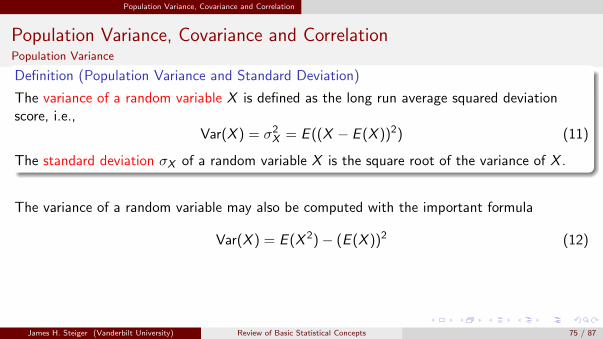
The variance of a random variable X is defined as the long run average squared deviationscore, i.e.,

Var(X ) = σ2X = E ((X − E (X ))2) (11)

The standard deviation σX of a random variable X is the square root of the variance of X .

The variance of a random variable may also be computed with the important formula

Var(X ) = E (X 2)− (E (X ))2 (12)



Population Variance, Covariance and CorrelationPopulation Covariance

Definition (Population Covariance)

The covariance of the random variables X and Y is defined as the long run averagecross-product of deviation scores, i.e.,

Cov(X ,Y ) = σX ,Y = E ((X − E (X ))(Y − E (Y ))) (13)

The covariance of X and Y may also be computed as

Cov(X ,Y ) = E (XY )− E (X )E (Y ) (14)



Population Variance, Covariance and CorrelationZ -Score Random Variables

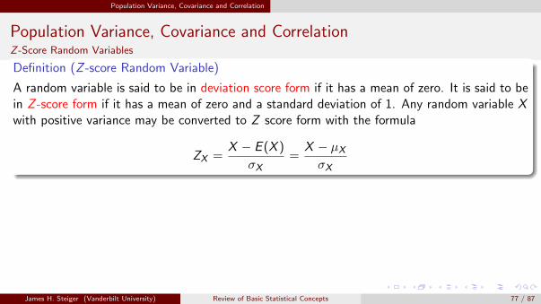
Definition (Z -score Random Variable)

A random variable is said to be in deviation score form if it has a mean of zero. It is said to bein Z -score form if it has a mean of zero and a standard deviation of 1. Any random variable Xwith positive variance may be converted to Z score form with the formula

ZX =X − E (X )

σX=

X − µXσX



Population Variance, Covariance and CorrelationPopulation Correlation

Definition (Population Correlation)

The correlation of random variables X and Y is defined as the long run average cross-productof Z scores, i.e.,

ρX ,Y = E (ZY ZY ) (15)

The correlation of X and Y may also be computed as

ρX ,Y =σX ,Y

σXσY(16)


Laws of Linear Combination

Laws of Linear CombinationDefinition (Linear Combination)

A linear combination of two random variables X and Y is any expression of the form aX + bYwhere a and b are constants called linear weights.



Laws of Linear CombinationMean of a Linear Combination

Theorem (Mean of a Linear Combination)

If random variables X and Y have means E (X ) and E (Y ), respectively, then the linearcombination aX + bY has mean E (aX + bY ) = aE (X ) + bE (Y ).

A similar result holds for linear combinations with sample data. That is, if X and Y representlists of numbers, and Wi = aXi + bYi , then W • = aX • + bY •.



Laws of Linear CombinationVariance of a Linear Combination

Theorem (Variance of a Linear Combination)

For random variables W ,X ,and Y , if W = aX + bY , then

σ2W = a2σ2

X + b2σ2Y + 2abσX ,Y

In a similar vein, for lists of numbers X and Y , if Wi = aXi + bYi , then

S2W = a2S2

X + b2S2Y + 2abSX ,Y



Laws of Linear CombinationThe General Heuristic Rule

Theorem (The General Heuristic Rule)

A general rule that allows computation of the variance of any linear combination ortransformation, as well as the covariance between any two linear transformations orcombinations, is the following:

For the variance of a single expression, write the expression, square it, and apply thesimple mnemonic conversion rule described below.For the covariance of any two expressions, write the two expressions, compute theiralgebraic product, then apply the conversion rule described below.

The conversion rule is as follows:

All constants are carried forward.If a term has the product of two variables, replace the product with the covariance of thetwo variables.If a term has the square of a single variable, replace the squared variable with its variance.Any term without the product of two variables or the square of a variable is deleted.




Example (The General Heuristic Rule)

Suppose X and Y are random variables, and you compute the following new random variables:

W = X − YM = 2X + 5

Construct formulas for

1 σ2W

2 σ2M

3 σW ,M

(Answers on next slide . . . )




Example (The General Heuristic Rule)

Answers.

1 To get σ2W , we square X − Y , obtaining X 2 + Y 2 − 2XY , and apply the conversion rule

to get σ2W = σ2

X + σ2Y − 2σX ,Y .

2 To get σ2M , we square 2X + 5, obtaining 4X 2 + 20X + 25. Applying the conversion rule,

we drop the last two terms, neither of which have the square of a variable or the productof two variables. We are left with the first term, which yields σ2

M = 4σ2X .

3 To get σW ,M , we begin by computing (X − Y )(2X + 5) = 2X 2 − 2XY + 5X − 5Y . Wedrop the last two terms, and obtain σW ,M = 2σ2

X − 2σX ,Y .


Significance Test for the Correlation Coefficient

Significance Test for r

To test whether Pearson correlation r is significantly different from zero, use the followingt statistic, which has n − 2 degrees of freedom. Of course, the statistical null hypothesisis that the population correlation ρ = 0.

tn−2 =√

n − 2r√

1− r 2(17)




Example (Significance Test for r)

Suppose you observe a correlation coefficient of 0.2371 with a sample of n = 93. Can youreject the null hypothesis that ρ = 0? Use α = 0.05.




Example

Answer. We compute the t statistic with R.

> df <- 93 - 2

> t <- sqrt(df)*0.2371 / sqrt(1-0.2371^2)

> t

[1] 2.328177

> df

[1] 91

> t.crit <- qt(0.975,df) ## this command gets the 0.975 quantile of t

> t.crit

[1] 1.986377

Since the observed t exceeds the critical value, we can reject the null hypothesis and declarethe correlation statistically significant at the 0.05 level, two-tailed.


Documents

Review of Basic Statistical Concepts Notes/Covariance.pdf · Review of Basic Statistical Concepts James H. Steiger Department of Psychology and Human Development Vanderbilt University