Notes on Electro-Optics

Review of Basic Principles of

Electromagnetic Fields

Prof. Elias N. GlytsisOctober 13, 2021

School of Electrical & Computer Engineering

National Technical University of Athens

This page was intentionally left blank......

Contents

1 Review of Maxwell’s Equations 1

2 Plane Wave Solutions 4

2.1 Isotropic Materials . . . . . . . . . . . . . . . . . . . . . . . . . . . . . . . . . . 42.2 Anisotropic Materials . . . . . . . . . . . . . . . . . . . . . . . . . . . . . . . . . 62.3 The Index Ellipsoid . . . . . . . . . . . . . . . . . . . . . . . . . . . . . . . . . . 9

3 Reflection and Transmission at a Planar Boundary 13

4 Electromagnetic Field Energy and Power - Poynting’s Theorem 19

5 Generalized Reflection and Transmission at a Planar Boundary 24

6 Jones Calculus 27

References 31

3

This page was intentionally left blank......

REVIEW OF BASIC PRINCIPLES OF

ELECTROMAGNETIC FIELDS †

1. Review of Maxwell’s Equations

The basis of electromagnetic fields theory are Maxwell’s equations. These equations describe

how the electromagnetic fields are coupled together and are related to the electric charges and

currents (which are the sources of the electromagnetic fields). The most common representation

of the Maxwell’s equations is the following:

~∇× ~E = −∂~B∂t, (1)

~∇× ~H = ~J +∂ ~D∂t, (2)

~∇ · ~D = ρ, (3)

~∇ · ~B = 0, (4)

where ~E(~r, t) represents the electric field (in V/m), ~D(~r, t) represents the displacement vector

(or the electric flux density vector in C/m), ~H(~r, t) represents the magnetic field (in A/m),

~B(~r, t) represents the magnetic flux density (in Tesla = Wb/m2), ~J (~r, t) represents the electric

current density (in A/m2),and ρ(~r, t) represents the electric charge density (in C/m3). The

above equations are written in the form of differential equations while an integral form can also

be used. In the integral form the Maxwell’s equations are written as follows:∮

C

~E · d~ = − d

dt

∫∫

S

~B · d~S, (Faraday Law), (5)

∮

C

~H · d~ =

∫

S

~J · d~S +d

dt

∫∫

S

~D · d~S, (Ampere Law), (6)

∫∫

S

© ~D · d~S =

∫∫∫

V

ρdV, (Gauss Law), (7)

∫∫

S

© ~B · d~S = 0, (Absence of Magnetic Monopoles), (8)

where in the first two equations C is a closed contour and S is a surface ending in that contour,

while the orientation of its unit vector is compatible with the right-hand rule when the direction

that the contour is traced. In the last two of the above integral equations, S is a closed surface

that defines a volume V and its unit vector points away from the surface.

† c©2021 Prof. Elias N. Glytsis, Last Update: October 13, 2021

1

In space with various materials parameters, the differential form of the Maxwell’s equations

requires the use of boundary conditions between the electromagnetics fields, when they are

used at the boundaries between various media. The boundary conditions in electromagnetics

can be easily derived from the integral form of Maxwell’s equations by shrinking the contours,

surfaces, and volumes to points on the boundary between differing regions. Then the resulting

equations, known as boundary conditions, are the following:

in × (~E+ − ~E−)S = 0, (9)

in × ( ~H+ − ~H−)S = ~K, (10)

in · ( ~D+ − ~D−)S = σ, (11)

in · ( ~B+ − ~B−)S = 0, (12)

where ~K is the possible surface current density (in A/m) and σ is the possible surface charge

density (in C/m2) on the boundary, respectively. The in is the unit vector normal to the

boundary and pointing to the + region (Fig. 1).

�

� � � � � � �� � � �

Figure 1: Boundary between two media denoted by “+” and “−” respectively.

Another equation that can be derived from Maxwell’s equations is the continuity equa-

tion (conservation of electric charge) that can be written in the following form (differential or

integral)

~∇ · ~J +∂ρ

∂t= 0 ⇐⇒

∫∫

S

© ~J · d~S +d

dt

∫∫∫

V

ρdV = 0, (13)

while the corresponding boundary condition is

in · ( ~J+ − ~J−)S = −~∇2 · ~K− ∂σ

∂t, (14)

and ~∇2 · ~K denotes the two-dimensional divergence of the current density.

Maxwell’s equations can also be written in the time-harmonic form where phasors are used.

For example the real electric field, ~E(~r, t), and its phasor representation, ~E(~r, ω), are related by~E(~r, t) = Re{ ~E(~r, ω) exp(jωt)}, where ω is the radial (angular) frequency of the electromagnetic

field. The same phasor representation can be used for all the electromagnetic fields and sources.

2

The phasor representation can be thought as a special case of the Fourier transform of the a

sinusoidal time varying electromagnetic field. Using either the Fourier transform of Eqs. (1)-(4)

or their phasor representation they can be written in the following time-harmonic form:

~∇× ~E(~r, ω) = −jω ~B(~r, ω), (15)

~∇× ~H(~r, ω) = ~J(~r, ω) + jω ~D(~r, ω), (16)

~∇ · ~D(~r, ω) = ρ(~r, ω), (17)

~∇ · ~B(~r, ω) = 0. (18)

The electromagnetic fields are also related via the constitutive equations. For example, in

freespace, the constitutive equations are

~D(~r, t) = ε0~E(~r, t) ⇐⇒ ~D(~r, ω) = ε0 ~E(~r, ω), (19)

~B(~r, t) = µ0~H(~r, t) ⇐⇒ ~B(~r, ω) = µ0

~H(~r, ω), (20)

where ε0 = 8.854187817 × 10−12 F/m is the permittivity and µ0 = 4π × 10−7 H/m is the

permeability, respectively, of freespace. For a linear, homogeneous, isotropic medium the mate-

rial response through the polarization, magnetization (and for conductive material conductiv-

ity/resistance) have to be taken into account. The relation between the material polarization

and magnetization and the electromagnetic fields can be written in the form (for linear, homo-

geneous, and isotropic media)

~P(~r, t) = ε0

∫ ∞

0

Ge(τ )~E(~r, t− τ )dτ ⇐⇒ ~P (~r, ω) = ε0χe(ω) ~E(~r, ω), (21)

~M(~r, t) =

∫ ∞

0

Gm(τ ) ~H(~r, t− τ )dτ ⇐⇒ ~M(~r, ω) = χm(ω) ~H(~r, ω), (22)

~J (~r, t) =

∫ ∞

0

Gc(τ )~E(~r, t− τ )dτ ⇐⇒ ~J(~r, ω) = σ(ω) ~E(~r, ω), (23)

where Ge, Gm, and Gc are kernels that describe the material memory of the electromagnetic

fields (the intervals from 0 to ∞ take into account the causality of the material, i.e. the polariza-

tion, for example, cannot depend on future values of the electric field). The parameters χe, χm,

and σ define the electric susceptibility, the magnetic susceptibility, and the conductivity of the

material (these are actually the Fourier transforms of the kernels Ge, Gm, and Gc respectively).

Using the above equations in the frequency domain the following constitutive equations can be

written:

~D(~r, ω) = ε0 ~E(~r, ω) + ~P (~r, ω) = ε0 [1 + χe(ω)] ~E(~r, ω) = ε(ω) ~E(~r, ω), (24)

~B(~r, ω) = µ0[ ~H(~r, ω) + ~M (~r, ω)] = µ0 [1 + χm(ω)] ~H(~r, ω) = µ(ω) ~H(~r, ω), (25)

~J(~r, ω) = σ(ω) ~E(~r, ω), (26)

3

where ε(ω) = ε0(1 + χe) = ε0εr(ω) is the material permittivity and εr is the material relative

permittivity. The material permeability is µ(ω) = µ0(1 + χm) = µ0µr(ω) and µr is its relative

permeability. The dependence of the materials macroscopic parameters (permittivity, perme-

ability, conductivity) on the frequency denotes what is called dispersion. All real materials

have dispersion. Ideally, when a material is considered as dispersion free, then its macroscopic

parameters are frequency independent and Eqs. (24)-(26) are also valid in the time domain.

When a material is linear, homogeneous, and anisotropic then the constitutive equations

can be written in the form

~D(~r, ω) = ε(ω) ~E(~r, ω), (27)

~B(~r, ω) = µ(ω) ~H(~r, ω), (28)

~J(~r, ω) = σ(ω) ~E(~r, ω), (29)

where ε, µ, and σ are the permittivity, permeability, and conductivity tensors (3 × 3 matri-

ces in this case). Even more complex constitutive equations can describe real materials such

as bianisotropic materials (where ~D depends on both ~E and ~H and in analogous manner ~B

depends on both ~H and ~E). Furthermore, except being anisotropic (or bianisotropic), disper-

sive (or non-dispersive) a material can also be inhomogeneous and/or nonlinear. In the case

of the inhomogeneity the macroscopic parameters are spatially dependent (an example would

be a holographic grating region). In the case of a nonlinear material the polarization, and/or

magnetization and/or conductivity depend nonlinearly on the electromagnetic fields.

2. Plane Wave Solutions

2.1 Isotropic Materials

In this section it is assumed that the materials of interest are lossless dielectrics (of zero con-

ductivity, i.e. σ = 0). In addition, it is assumed that there are no sources (electric charges,

ρ = 0 and electric currents, ~J = 0). This actually means that the electromagnetic fields were

generated at infinite distance away from the areas of interest. Furthermore, it is assumed that

all media are linear, homogeneous, isotropic, and nonmagnetic (common for optical materials).

Solutions of the form (time-harmonic) ~E(~r, ω) = ~E0 exp(−j~k · ~r) are sought (phasors). The

real field can be determined from ~E(~r, t) = Re{ ~E0 exp(−j~k ·~r) exp(jωt)}. This form of solution

for the electric field constitutes a plane wave because the locus of constant phase (wavefront)

is an infinite plane perpendicular to the direction of propagation that is defined through the

wavevector ~k. Using also the constitutive equations [Eqs. (24) and (25)] Maxwell’s equations

4

can be written in the following form:

~k × ~E = ωµ0~H, (30)

~k × ~H = −ωε0εr~E, (31)

~k · ~E = 0, (32)

~k · ~H = 0. (33)

By eliminating the magnetic field from the above equations it is straightforward to show that

the following equation should be satisfied

[

~k · ~k − ω2ε0µ0n2]

~E = 0, (34)

where n2 = εr with n defined as the index of refraction of the material. Equation (34) is actually

the wave equation for the case of plane wave solutions in the time harmonic form. Of course,

in order for Eq. (34) to have nontrivial solutions it is necessary that the following dispersion

equation be satisfied~k · ~k − ω2ε0µ0n

2 = ~k · ~k − k20n

2 = 0, (35)

where k0 = ω√ε0µ0 = ω/c = 2π/λ0, with k0, c, λ0 being the freespace wavenumber, the

freespace light velocity, and the freespace wavelength, respectively.

�

��

�

�

� � � � � � �

Figure 2: A plane wave dispersion sphere of radius |~k| = k0n. The electric field, the magnetic field, and the

wavevector form a right-handed orthogonal system.

As it is implied from Eqs. (30)-(33) the electric field, the magnetic field, and the wavevector

form a right-handed orthogonal system of vectors. Furthermore, Eq. (35) represents a sphere

in wavevector space of radius k0n. I.e., for any direction of propagation of an electromagnetic

5

wave in an isotropic, homogeneous, and linear medium the index of refraction is constant while

the polarization remains perpendicular to the direction of propagation. The wavevector surface

(sphere) is shown in Fig. 2. For the latter reason, usually two orthogonal polarizations are

recognized which are called eigen-polarizations since they propagate inside the medium without

being altered. For isotropic media the selection of the two orthogonal polarizations is arbitrary

since there are infinite pairs of orthogonal polarizations for each direction of propagation. This

situation changes dramatically in the case of anisotropic materials.

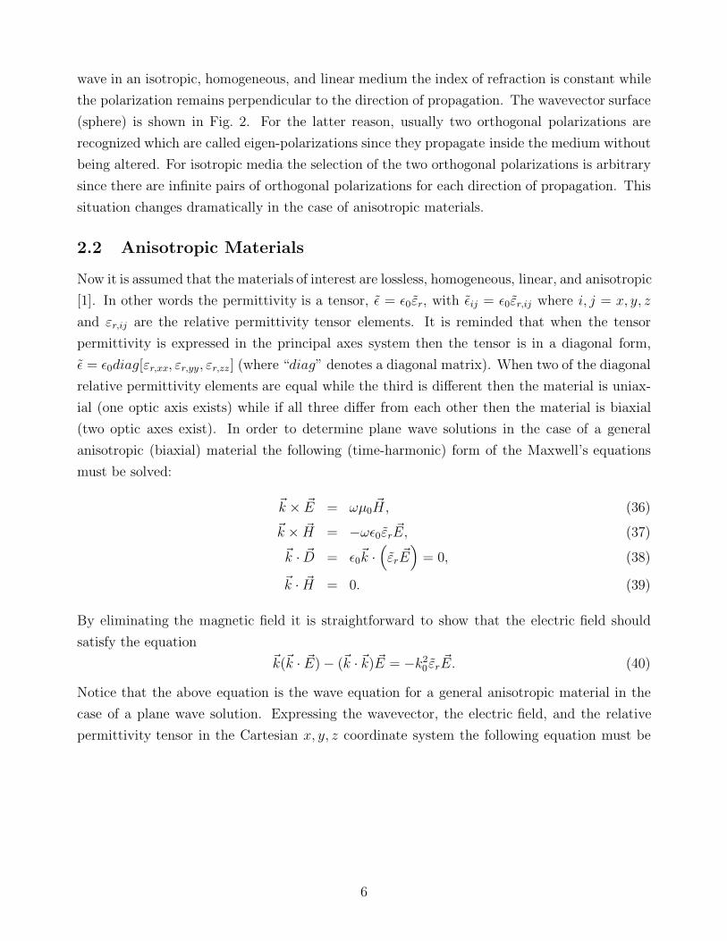
2.2 Anisotropic Materials

Now it is assumed that the materials of interest are lossless, homogeneous, linear, and anisotropic

[1]. In other words the permittivity is a tensor, ε = ε0εr, with εij = ε0εr,ij where i, j = x, y, z

and εr,ij are the relative permittivity tensor elements. It is reminded that when the tensor

permittivity is expressed in the principal axes system then the tensor is in a diagonal form,

ε = ε0diag[εr,xx, εr,yy, εr,zz] (where “diag” denotes a diagonal matrix). When two of the diagonal

relative permittivity elements are equal while the third is different then the material is uniax-

ial (one optic axis exists) while if all three differ from each other then the material is biaxial

(two optic axes exist). In order to determine plane wave solutions in the case of a general

anisotropic (biaxial) material the following (time-harmonic) form of the Maxwell’s equations

must be solved:

~k × ~E = ωµ0~H, (36)

~k × ~H = −ωε0εr~E, (37)

~k · ~D = ε0~k ·(

εr~E)

= 0, (38)

~k · ~H = 0. (39)

By eliminating the magnetic field it is straightforward to show that the electric field should

satisfy the equation~k(~k · ~E) − (~k · ~k) ~E = −k2

0 εr~E. (40)

Notice that the above equation is the wave equation for a general anisotropic material in the

case of a plane wave solution. Expressing the wavevector, the electric field, and the relative

permittivity tensor in the Cartesian x, y, z coordinate system the following equation must be

6

satisfied:

k20εr,xx − (k2

y + k2z) kxky + k2

0εr,xy kxkz + k20εr,xz

kykx + k20εr,yx k2

0εr,yy − (k2x + k2

z) kykz + k20εr,yz

kzkx + k20εr,zx kzky + k2

0εr,zy k20εr,zz − (k2

x + k2y)

Ex

Ey

Ez

= 0 =⇒

=⇒[

A(kx, ky, kz)]

Ex

Ey

Ez

= 0. (41)

2

x-wavevector (k x/k 0

)

εxx

= 1, εyy

= 2, εzz

= 4, εxy

= 0, εxz

= 0, εyz

= 0, λ0 = 1 µm

1

00

y-wavevector (ky /k

0 )

0.5

1

1.5

0

0.5

1

2

z-w

avevecto

r (k

z/k

0)

x-wavevector (k x/k 0

)

2

εxx

= 1, εyy

= 2, εzz

= 4, εxy

= 0, εxz

= 0, εyz

= 0, λ0 = 1 µm

1

0-2

-1

y-wavevector (ky /k

0 )

0

1

0

0.5

1

2

z-w

avevecto

r (k

z/k

0)

(a) (b)

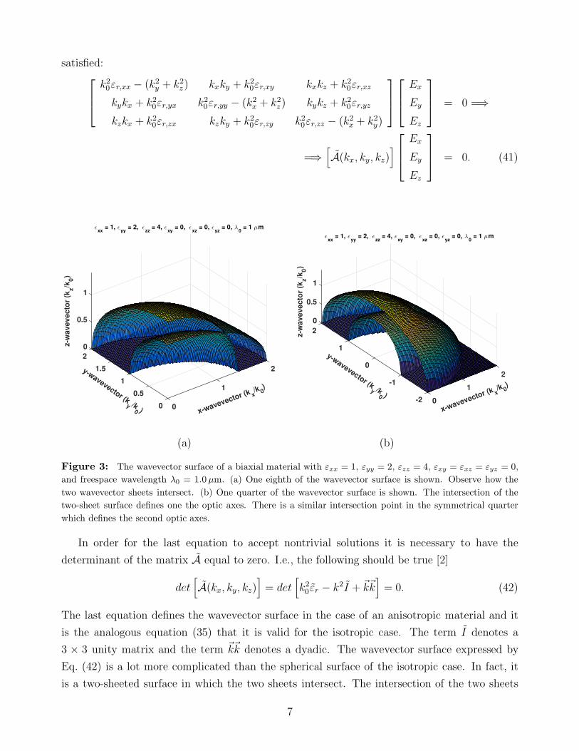
Figure 3: The wavevector surface of a biaxial material with εxx = 1, εyy = 2, εzz = 4, εxy = εxz = εyz = 0,

and freespace wavelength λ0 = 1.0µm. (a) One eighth of the wavevector surface is shown. Observe how the

two wavevector sheets intersect. (b) One quarter of the wavevector surface is shown. The intersection of the

two-sheet surface defines one the optic axes. There is a similar intersection point in the symmetrical quarter

which defines the second optic axes.

In order for the last equation to accept nontrivial solutions it is necessary to have the

determinant of the matrix A equal to zero. I.e., the following should be true [2]

det[

A(kx, ky, kz)]

= det[

k20εr − k2I + ~k~k

]

= 0. (42)

The last equation defines the wavevector surface in the case of an anisotropic material and it

is the analogous equation (35) that it is valid for the isotropic case. The term I denotes a

3 × 3 unity matrix and the term ~k~k denotes a dyadic. The wavevector surface expressed by

Eq. (42) is a lot more complicated than the spherical surface of the isotropic case. In fact, it

is a two-sheeted surface in which the two sheets intersect. The intersection of the two sheets

7

define the two optic axis. To have a better understanding a sample case is shown in Fig. 3.

For each wavevector (kx, ky, kz) that satisfies Eq. (42) the corresponding refractive index can be

found as n =√

k2x + k2

y + k2z/k0 while the corresponding polarization of the electric field vector

can be determined from the null space of matrix A(kx, ky, kz). Specifically, if the wavevector is

expressed in the rectangular coordinate system, with the azimuthal and polar angles (φ and θ)

specifying its direction, then

~k = k0n(axx+ ayy + azz) = k0n(sin θ cos φ x+ sin θ sinφ y + cos θ z), (43)

where n is refractive index that the plane wave experiences when is propagating through the

medium at the specified direction. By replacing the wavevector components from Eq.(43) into

Eq. (42) the following bi-quadratic equation for n can be derived

An4 +Bn2 + C = 0, where, (44)

A = a4xεr,xx + a4

yεr,yy + a4zεr,zz + a2

xa2yεr,xx + a2

xa2zεr,xx + a2

xa2yεr,yy + a2

ya2zεr,yy

a2xa

2zεr,zz + a2

ya2zεr,zz + 2axa

3yεr,xy + 2a3

xayεr,xy + 2axa3zεr,xz + 2a3

xazεr,xz

+2aya3zεr,yz + 2a3

yazεr,yz + 2axaya2zεr,xy + 2axa

2yazεr,xz + 2a2

xayazεr,yz,

B = −a2xεr,xxεr,yy + a2

xε2r,xz + a2

yε2r,xy + a2

yε2r,yz + a2

zε2r,xz + a2

zε2r,yz + a2

xε2r,xy − a2

yεr,xxεr,yy

−a2xεr,xxεr,zz − a2

zεr,xxεr,zz − a2yεr,yyεr,zz − a2

zεr,yyεr,zz + 2axayεr,xzεr,yz − 2axayεr,xyεr,zz

+2axazεr,xyεr,yz − 2axazεr,xzεr,yy + 2ayazεr,xyεr,xz − 2ayazεr,xxεr,yz ,

C = εr,xxεr,yyεr,zz − εr,zzε2r,xy + 2εr,xyεr,xzεr,yz − εr,yyε

2r,xz − εr,xxε

2r,yz .

Equation (44) always has two real positive solutions that correspond to the two extraordidary

waves that can propagate for each specified direction. The polarization of the correspond-

ing electric field can be found from Eq. (41). It is reminded that the ~D eigenvectors are

perpendicular to each other. The previous equation can be simplified if the relative permit-

tivity is expressed in the principal axis system and all the off-diagonal elements become zero

(εr,xy = εr,xz = εr,yz = 0). In the latter case Eq. (44) can be written

a2xn

2(n2 − εr,yy)(n2 − εr,zz) + a2

yn2(n2 − εr,xx)(n

2 − εr,zz) + a2zn

2(n2 − εr,xx)(n2 − εr,yy)

= (n2 − εr,xx)(n2 − εr,yy)(n

2 − εr,zz), (45)

and the last equation can be expressed in the most common compact form [1]

a2x

n2 − εr,xx+

a2y

n2 − εr,yy+

a2z

n2 − εr,zz=

1

n2, (46)

though the latter equation cannot be used along the principal axes of the coordinate system.

In the case of a uniaxial material the permittivity tensor can be written (in the principal axis

system) as ε = ε0diag[εO, εO, εE ] = ε0diag[n2O, n

2O, n

2E ] where nO and nE are the ordinary and

8

the principal extraordinary refractive index respectively. The direction of the unique optic axis

is denoted by the unit vector c = cxx+ cy y+ cz z. By decomposing all vectors in Eqs. (36)-(39)

into a component along the optic axis and one transverse to the optic axis (for example for

electric field Ec, and ~Et respectively), they can be written in the following form [3]

(~kt × c)Ec + kc(c× ~Et) = ωµ0~Ht, (47)

~kt × ~Et = ωµ0Hcc, (48)

(~kt × c)Hc + kc(c× ~Ht) = −ωε0n2O~Et, (49)

~kt × ~Ht = −ωε0n2EEcc, (50)

n2O~kt · ~Et + n2

EkcEc = 0, (51)

~kt · ~Ht + kcHc = 0. (52)

Manipulating the above equations it is straightforward to derive the wavevector surface equation

equivalent to Eq. (42) for the uniaxial material. This is written as follows

[~k · ~k − k20n

2O][n2

O~k · ~k + (n2

E − n2O)(~k · c)2 − k2

0n2On

2E ] = 0. (53)

From Eq. (53) the two possible solutions are evident while the corresponding polarizations are

given as follows

~k · ~k − k20n

2O = 0 =⇒ ~E · c = 0, ordinary wave, (54)

n2O~k · ~k + (n2

E − n2O)(~k · c)2 − k2

0n2On

2E = 0, =⇒ ~H · c = 0 extraordinary wave. (55)

To have a better understanding a sample case is shown in Fig. 4 which is similar to Fig. 3 but

for a uniaxial material.

Half of the wavevector surfaces along with their optic axes are shown in Fig. 5a and 5b for

the biaxial and uniaxial cases presented previously.

For comparison purposes similar figures to Figs. 3 and 4 are given in Fig. 6 for an isotropic

material of unity relative permittivity.

2.3 The Index Ellipsoid

The index ellipsoid is used to determine the eigen-polarizations and the corresponding indices of

refraction for a given direction of propagation in an anisotropic crystal. The index ellipsoid (or

optical indicatrix) represents a normalized surface of constant electromagnetic energy density.

It is known (it is reviewed in a later section) that in a homogeneous, lossless, and linear medium

(dielectric in this case) the electromagnetic energy density is given by 〈wem〉 = (1/4)Re{ ~E ·~D∗} = (1/4) ~E · ~D∗ (where ~E and ~D are the phasors of the electric field and the dielectric

displacement, respectively). Replacing ~E = ε−10 [εr]

−1 ~D the electromagnetic energy density can

be written as (expressed in the principal axes system)

9

1.5

εxx

= 1, εyy

= 1, εzz

= 2.25, εxy

= 0, εxz

= 0, εyz

= 0, λ0 = 1 µm

x-wavevector (k x/k 0

)1

0.5

00

y-wavevector (ky /k

0 )

0.5

1

0.2

0

0.8

0.6

0.4

1.5

z-w

avevecto

r (k

z/k

0)

x-wavevector (k x/k 0

)

1.5

εxx

= 1, εyy

= 1, εzz

= 2.25, εxy

= 0, εxz

= 0, εyz

= 0, λ0 = 1 µm

1

0.5

0-1.5

-1

-0.5

y-wavevector (ky /k

0 )

0

0.5

1

0

0.5

1

1.5z-w

avevecto

r (k

z/k

0)

(a) (b)

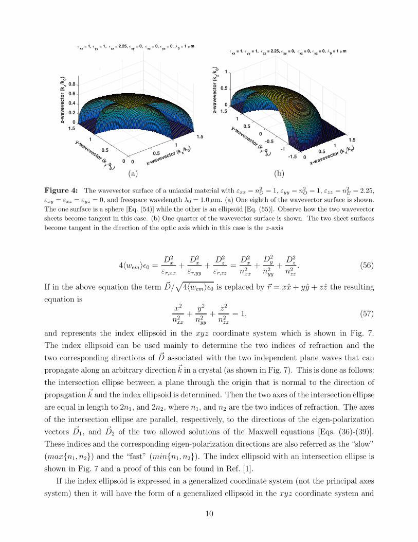
Figure 4: The wavevector surface of a uniaxial material with εxx = n2

O = 1, εyy = n2

O = 1, εzz = n2

E = 2.25,

εxy = εxz = εyz = 0, and freespace wavelength λ0 = 1.0µm. (a) One eighth of the wavevector surface is shown.

The one surface is a sphere [Eq. (54)] while the other is an ellipsoid [Eq. (55)]. Observe how the two wavevector

sheets become tangent in this case. (b) One quarter of the wavevector surface is shown. The two-sheet surfaces

become tangent in the direction of the optic axis which in this case is the z-axis

4〈wem〉ε0 =D2

x

εr,xx+

D2x

εr,yy+

D2z

εr,zz=D2

x

n2xx

+D2

y

n2yy

+D2

z

n2zz

. (56)

If in the above equation the term ~D/√

4〈wem〉ε0 is replaced by ~r = xx+ yy + zz the resulting

equation isx2

n2xx

+y2

n2yy

+z2

n2zz

= 1, (57)

and represents the index ellipsoid in the xyz coordinate system which is shown in Fig. 7.

The index ellipsoid can be used mainly to determine the two indices of refraction and the

two corresponding directions of ~D associated with the two independent plane waves that can

propagate along an arbitrary direction ~k in a crystal (as shown in Fig. 7). This is done as follows:

the intersection ellipse between a plane through the origin that is normal to the direction of

propagation ~k and the index ellipsoid is determined. Then the two axes of the intersection ellipse

are equal in length to 2n1, and 2n2, where n1, and n2 are the two indices of refraction. The axes

of the intersection ellipse are parallel, respectively, to the directions of the eigen-polarization

vectors ~D1, and ~D2 of the two allowed solutions of the Maxwell equations [Eqs. (36)-(39)].

These indices and the corresponding eigen-polarization directions are also referred as the “slow”

(max{n1, n2}) and the “fast” (min{n1, n2}). The index ellipsoid with an intersection ellipse is

shown in Fig. 7 and a proof of this can be found in Ref. [1].

If the index ellipsoid is expressed in a generalized coordinate system (not the principal axes

system) then it will have the form of a generalized ellipsoid in the xyz coordinate system and

10

(a) (b)

Figure 5: (a) The wavevector surface of a biaxial material with εxx = 1, εyy = 2, εzz = 4, εxy = εxz = εyz = 0,

and freespace wavelength λ0 = 1.0µm. Half of the wavevector surface is shown. Observe the two wavevector

sheets that intersect in four points that define the two optic axes of the biaxial material. (b) The wavevector

surface of a uniaxial material with εxx = 1, εyy = 1, εzz = 2.25, εxy = εxz = εyz = 0, and freespace wavelength

λ0 = 1.0µm. Half of the wavevector surface is shown. Observe the ellipsoidal and spherical wavevector sheets

that touch only in two points where the single optic axis is defined.

εxx

= 1, εyy

= 1, εzz

= 1, εxy

= 0, εxz

= 0, εyz

= 0, λ0 = 1 µm

1

x-wavevector (k x/k 0

)0.5

00

y-wavevector (ky /k

0 )

0.5

0

0.2

0.4

0.6

0.8

1

z-w

avevecto

r (k

z/k

0)

x-wavevector (k x/k 0

)1

εxx

= 1, εyy

= 1, εzz

= 1, εxy

= 0, εxz

= 0, εyz

= 0, λ0 = 1 µm

0.5

0-1

-0.5

y-wavevector (ky /k

0 )

0

0.5

0

0.5

1

1

z-w

avevecto

r (k

z/k

0)

(a) (b)

Figure 6: The wavevector surface of an isotropic material with ε = n2 = 1, and freespace wavelength

λ0 = 1.0µm. (a) One eighth of the wavevector surface is shown. The two-sheeted surface collapses to a single

spherical surface. (b) One quarter of the wavevector surface is shown.

11

�

� �

�� !"

# $% & ' ( () * *

+ , ,

Figure 7: The index ellipsoid in the general biaxial case where nxx 6= nyy 6= nzz 6= nxx, shown in the

principal axes system. A random direction of a plane wave wavevector is also shown. The intersection of the

plane perpendicular to the wavevector forms an ellipse with its axes specifying the two eigenpolarizations ~D1

and ~D2 with n1 and n2 (semi-axes of the ellipse) the corresponding refractive indices.

its equation is given by

[

x y z]T

[A]

xyz

=[

x y z]T

1n2

xx

1n2

xy

1n2

xz

1n2

yx

1n2

yy

1n2

yz1

n2zx

1n2

zy

1n2

zz

xyz

= 1, (58)

where A = [εr]−1 is the impermeability matrix. It is reminded that the impermeability matrix

is also symmetric since is the inverse of the symmetric relative permittivity matrix (nuv = nvu,

where u 6= v and u, v = x, y, z).

In the case of uniaxial material where nxx = nyy = nO (ordinary index) and nzz = nE

(extraordinary index), the index ellipsoid is an ellispoid of revolution around z axis (optic

axis). In the latter case, if the direction of the electromagnetic wavevector forms an angle θ

with the optic axis, the extraordinary refractive index, ne(θ) is given by

cos2 θ

n2O

+sin2 θ

n2E

=1

n2e(θ)

, (59)

while of course the ordinary index remains always nO.

12

3. Reflection and Transmission at a Planar Boundary

In this section the reflection and transmission of a plane wave at a planar boundary between two

isotropic dielectrics will be reviewed. In Fig. 8 the boundary (xz plane) between two dielectrics

of permittivities ε1 = ε0εr1 = ε0n21 and ε2 = ε0εr2 = ε0n

22 is shown. A plane wave is incident

at angle θ1 on the boundary and a reflected as well as a transmitted wave are induced. The

electric field in region 1 (left) and region 2 (right) can be written as follows

- . / 0 1

2 3

4 5 6 7 8

9

:; <

= > ? @ A B C D E B F D @ G= H ? @ A B C D E B F D @ G

I J

K LM NO P

Figure 8: A planar boundary between two isotropic, nonmagnetic, dielectrics with permittivities ε1 and ε2.

The green electric field direction (along the y-axis) corresponds to the TE polarization, while the blue electric

field direction (in the xz-plane) corresponds to the TM polarization. The angle of incidence is θ1, the angle of

reflection is θr = θ1, and the angle of refraction is θ2.

~E1 = ~Ei exp(−j~ki · ~r) + ~Er exp(−j~kr · ~r), (60)

~H1 =1

ωµ0

(

~ki × ~Ei

)

exp(−j~ki · ~r) +1

ωµ0

(

~kr × ~Er

)

exp(−j~kr · ~r), (61)

~E2 = ~Et exp(−j~kt · ~r), (62)

~H2 =1

ωµ0

(

~kt × ~Et

)

exp(−j~kt · ~r), (63)

where ~Ei, ~Er, and ~Et correspond to the incident, reflected, and transmitted electric field ampli-

tudes, while ~ki, ~kr, and ~kt correspond to the incident, reflected, and transmitted wavevectors.

Of course the wavevectors satisfy Eq. (35) for each of the regions of interest. Using the continu-

ity of the tangential to the boundary electric field components the following necessary condition

13

must be satisfied:

(~ki · ~r)z=0 = (~kr · ~r)z=0 = (~kt · ~r)z=0 =⇒ kix = krx = ktx =⇒k0n1 sin θ1 = k0n1 sin θr = k0n2 sin θ2. (64)

The last equation is the well known phase matching condition. From the phase matching

condition it is evident that θr = θ1 (reflection angle equals incident angle) and n1 sin θ1 =

n2 sin θ2 (Snell’s law). Of course in order to find the unknown amplitude coefficients for the

reflected and the transmitted waves the full form of the boundary condition should be used

in conjunction with the analogous boundary condition for the magnetic field. Usually, any

incident polarization for the incident field can be decomposed into one that the electric field is

perpendicular to the plane of incidence (xz plane here) which is referred as ⊥ or TE polarization,

and one that the electric field is parallel to the plane of incidence which is referred as ‖ or TM

polarization. A generalized polarization formulation is presented in a later section. These two

orthogonal polarizations are decoupled in the case of the isotropic media and can be studied

independently. Solving the boundary conditions the unknown amplitudes of the reflected and

of the transmitted fields can be determined. These are generally expressed in the form of the

Fresnel equations which are shown below:

rTE

= r⊥ =Er

Ei=

n1 cos θ1 − n2 cos θ2

n1 cos θ1 + n2 cos θ2, (65)

tTE

= t⊥ =Et

Ei=

2n1 cos θ1

n1 cos θ1 + n2 cos θ2, (66)

rTM

= r‖ =Er

Ei=

n2 cos θ1 − n1 cos θ2

n2 cos θ1 + n1 cos θ2, (67)

tTM

= t‖ =Et

Ei=

2n1 cos θ1

n2 cos θ1 + n1 cos θ2. (68)

There are some interesting points to be discussed in the case of the Fresnel equations.

Initially, it is assumed that n1 < n2 (for example from air to glass). In this case the wavevector

diagram of Fig. 9a is valid. The phase matching condition is also shown in this figure. For

this case the Brewster angle can also be defined as the angle for which the reflected wave

vanishes. For nonmagnetic materials this can occur only in the case of TM (‖) polarization,

and it is defined as rTM

(θ1 = θB) = 0 =⇒ θB = tan−1(n2/n1). As an example, the reflection

and transmission coefficients are shown in Figs. 10 and 11 as functions of the angle of incidence

θ1 for the case of n1 = 1.0 and n2 = 1.5.

The situation becomes more interesting when n1 > n2 (for example from glass to air). In

this case the Brewster angle is defined in a similar manner as before and it exists only for TM

polarization. However, in this case, for both polarizations the critical angle can be defined.

14

Q

R

S T U VW X

Y Z [ \] ^ _ ` a b c d b e ] ^ _ ` a b f d b g h b e

i

j

k l m n o pq r

s t u vw x y z { | } ~ | � w x y z { | � ~ | � � | �

(a) (b)

�

�

� � � �� � � �

� � � � � � � � � � � � � � � � � � � � � � �

(c)

Figure 9: The wavevector surface of an interface between two dielectrics. (a) Case of incidence from a low

to higher refractive index (n1 < n2). (b) Case of incidence from a high to a lower refractive index (n1 > n2)

and at θ1 = θcr . (c) Case of incidence from a high to a lower refractive index (n1 > n2) and at θ1 > θcr .

From Snell’s law the critical angle is defined as the angle of incidence for which the refraction

angle becomes 90 degrees. Therefore, the critical angle θcr is defined as θcr = sin−1(n2/n1).

In wavevector space this situation is depicted in Fig. 9b. In this situation due to the phase

matching condition [Eq. (64)] ktx = k0n2 and the z component of the transmitted wavevector

ktz becomes zero. In other words, the transmitted electric field, Eq. (62), is independent of

z. This can happen only in theory since exactly at the critical angle the transmitted field is

constant in region 2 which would require infinite energy from the electromagnetic field. The

practical case is when the angle of incidence is greater than the critical angle (θ1 > θcr). In the

15

Angle θ1 (deg)

0 20 40 60 80

|rT

E|

0

0.5

1

n1 = 1 n

2 = 1.5

Angle θ1 (deg)

0 20 40 60 80

Ph

ase o

f r T

E

-200

0

200n

1 = 1 n

2 = 1.5

Angle θ1 (deg)

0 20 40 60 80

|rT

M|

0

0.5

1

n1 = 1 n

2 = 1.5

Angle θ1 (deg)

0 20 40 60 80

Ph

ase o

f r T

M

-200

0

200n

1 = 1 n

2 = 1.5

Figure 10: Reflection coefficient as a function of the angle of incidence θ1 for TE and TM polarization in

the case of n1 < n2. The Brewster angle θB = tan−1(1.5/1) = 56.31◦ is obvious in the TM polarization case.

latter case from the phase matching condition it can be deduced

ktx = k0n1 sin θ1 > k0n1 sin θcr = k0n2. (69)

From the last equation and Eq. (35) for region 2 it is obvious that (for θ1 > θcr)

k2tz = k2

0n22 − k2

tx < 0 =⇒ ktz = ±j√

k2tx − k2

0n22 = ±jk0

√

n21 sin2 θ1 − n2

2 = ±jγt. (70)

This means that the z component of the transmitted wavevector becomes purely imaginary. In

the wavevector diagram this situation is depicted in Fig. 9c where the dashed purpled arrow

representing the transmitted wavevector is complex. There is some ambiguity in selecting the

sign of the right-hand side of Eq. (70). Since the transmitted field is expressed by Eq. (62), in

order to represent a physical field the “−” sign must be selected. Then Eq. (62) becomes

~E2 = ~Et exp[−k0

√

n21 sin2 θ1 − n2

2z] exp[−jxk0n1 sin θ1] = ~Ete−γtz exp[−jxk0n1 sin θ1]. (71)

The corresponding real field can be determined from the above phasor as (assuming for sim-

plicity that ~Ei is real)

~E2(x, z, t) = |t|Eiute−γtz cos [ωt− xk0n1 sin θ1 + φ(θ1)] , (72)

16

Angle θ1 (deg)

0 20 40 60 80

|tT

E|

0

0.2

0.4

0.6

n1 = 1 n

2 = 1.5

Angle θ1 (deg)

0 20 40 60 80

Ph

ase o

f t T

E

-200

0

200n

1 = 1 n

2 = 1.5

Angle θ1 (deg)

0 20 40 60 80

|tT

M|

0

0.2

0.4

0.6

n1 = 1 n

2 = 1.5

Angle θ1 (deg)

0 20 40 60 80

Ph

ase o

f t T

M

-200

0

200n

1 = 1 n

2 = 1.5

Figure 11: Transmission coefficient as a function of the angle of incidence θ1 for TE and TM polarization

in the case of n1 < n2.

where t = |t|ejφ is the complex transmission coefficient and ut is the unit vector of the trans-

mitted electric field. For example, ut = uTE

= y for TE polarization, and ut = utTM

=

cos θ2x− sin θ2z for TM polarization. However, in the TM polarization case utTM

has an imag-

inary component that should suitably (with the appropriate phase shift) be incorporated in

the latter equation of the real transmitted electric field. However, for simplicity, the form of

Eq. (72) does not take into account the complex component of ut. The latter form of the

transmitted field is called “evanescent field” or “evanescent wave.” It is easy to show that the

evanescent wave does not transfer real power in the z direction. This is the reason that this

situation is called total internal reflection since all the power is reflected back into the incident

region. An example evanescent field (its real part for t = 0 for TE polarization) is shown in

Fig. 12 for n1 = 1.5, n2 = 1.0, and θ = 65◦.

In the case of total internal reflection the reflection and transmission coefficients from Fresnel

equations become complex. It is interesting to define the reflection coefficients in this case which

17

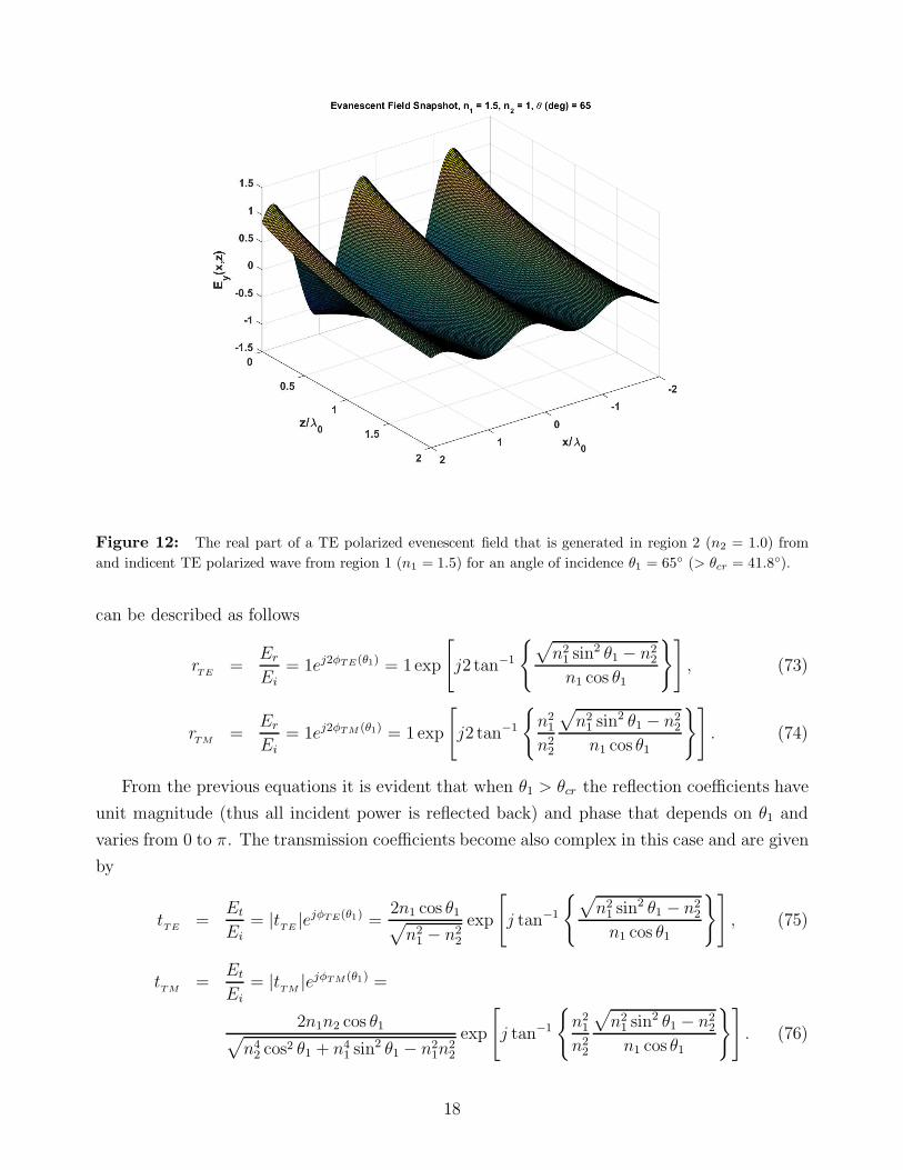
Figure 12: The real part of a TE polarized evenescent field that is generated in region 2 (n2 = 1.0) from

and indicent TE polarized wave from region 1 (n1 = 1.5) for an angle of incidence θ1 = 65◦ (> θcr = 41.8◦).

can be described as follows

rTE

=Er

Ei= 1ej2φTE(θ1) = 1exp

[

j2 tan−1

{

√

n21 sin2 θ1 − n2

2

n1 cos θ1

}]

, (73)

rTM

=Er

Ei= 1ej2φTM (θ1) = 1exp

[

j2 tan−1

{

n21

n22

√

n21 sin2 θ1 − n2

2

n1 cos θ1

}]

. (74)

From the previous equations it is evident that when θ1 > θcr the reflection coefficients have

unit magnitude (thus all incident power is reflected back) and phase that depends on θ1 and

varies from 0 to π. The transmission coefficients become also complex in this case and are given

by

tTE

=Et

Ei= |t

TE|ejφTE(θ1) =

2n1 cos θ1√

n21 − n2

2

exp

[

j tan−1

{

√

n21 sin2 θ1 − n2

2

n1 cos θ1

}]

, (75)

tTM

=Et

Ei

= |tTM

|ejφTM(θ1) =

2n1n2 cos θ1√

n42 cos2 θ1 + n4

1 sin2 θ1 − n21n

22

exp

[

j tan−1

{

n21

n22

√

n21 sin2 θ1 − n2

2

n1 cos θ1

}]

. (76)

18

Angle θ1 (deg)

0 20 40 60 80

|rT

E|

0

0.5

1

n1 = 1.5 n

2 = 1

Angle θ1 (deg)

0 20 40 60 80

Ph

ase o

f r T

E

-200

0

200n

1 = 1.5 n

2 = 1

Angle θ1 (deg)

0 20 40 60 80

|rT

M|

0

0.5

1

n1 = 1.5 n

2 = 1

Angle θ1 (deg)

0 20 40 60 80

Ph

ase o

f r T

M

-200

0

200n

1 = 1.5 n

2 = 1

Figure 13: Reflection coefficient as a function of the angle of incidence θ1 for TE and TM polarization in the

case of n1 > n2. The Brewster angle θB = tan−1(1/1.5) = 33.69◦ is obvious in the TM polarization case. For

both TE and TM polarization cases the critical angle θcr = sin−1(1/1.5) = 41.81◦ is also shown. For θ1 > θcr

the reflection coefficients become complex of unity magnitude and phase 2φTE(θ1) or 2φTM(θ1).

As an example, the reflection and transmission coefficients are shown in Figs. 13 and 14 as

functions of the angle of incidence θ1 for the case of n1 = 1.5 and n2 = 1.0.

4. Electromagnetic Field Energy and Power - Poynting’s

Theorem

From Maxwell’s equations [Eqs.(1)-(4)] it can be shown the following equality

−~∇ · (~E × ~H) = ~E · ~J + ~E · ∂~D∂t

+ ~H · ∂~B∂t

=

= ~E · ~J +∂

∂t

(ε02~E · ~E

)

+∂

∂t

(µ0

2~H · ~H

)

+ ~E · ∂~P∂t

+ µ0~H · ∂

~M∂t

, (77)

where the above equation represents the Poynting’s theorem in point form. In case that a closed

surface S is chosen, that encloses a volume V , the Poynting’s theorem can also be written in

19

Angle θ1 (deg)

0 20 40 60 80

|tT

E|

0

0.5

1

1.5

n1 = 1.5 n

2 = 1

Angle θ1 (deg)

0 20 40 60 80

Ph

ase o

f t T

E

-200

0

200n

1 = 1.5 n

2 = 1

Angle θ1 (deg)

0 20 40 60 80

|tT

M|

0

1

2

n1 = 1.5 n

2 = 1

Angle θ1 (deg)

0 20 40 60 80

Ph

ase o

f t T

M

-200

0

200n

1 = 1.5 n

2 = 1

Figure 14: Transmission coefficient as a function of the angle of incidence θ1 for TE and TM polarization

in the case of n1 > n2. For θ1 > θcr the transmission coefficient become complex.

its integral form as follows

−∫∫

S

©(

~E × ~H)

· d~S =

∫∫∫

V

~E · ~J dV +

∫∫∫

V

∂

∂t

(ε02~E · ~E +

µ0

2~H · ~H

)

dV +

∫∫∫

V

~E · ∂~P∂tdV +

∫∫∫

V

µ0~H · ∂

~M∂t

dV, (78)

where the vector ~N = ~E × ~H is defined as the Poynting vector (W/m2). The left-hand side

of Eq. (78) represents the total power entering the volume V via the closed surface S. The

right-hand sides represent the ohmic losses expended in volume V , the rate of increase of the

vacuum electromagnetic energy in volume V , the power expended in electric dipoles in volume

V , and the power expended in magnetic dipoles in volume V , respectively.

If the medium is linear in terms of its electric and magnetic properties, and experiences

negligible dispersion, then the electromagnetic energy density can be defined as

wem = we + wm =1

2

(

~E · ~D + ~H · ~B)

=1

2

(

ε|~E|2 + µ| ~H|2)

. (79)

20

Then Eqs. (77) and (78) can be written in the following forms

−~∇ ·(

~E × ~H)

= ~E · ~J +∂wem

∂t, (80)

−∫∫

S

©(

~E × ~H)

· d~S =

∫∫∫

V

[

~E · ~J +∂wem

∂t

]

dV. (81)

The physical meaning of the differential or integral form of Eqs. (80) or (81) is that the

time rate of change of electromagnetic energy within a certain volume, plus the total work done

by the fields on the sources within the volume, is equal to the energy flowing in through the

boundary surfaces of the volume per unit time. This is the statement of conservation of energy.

Of course the case of a dispersionless medium is ideal. All real materials have dispersion

(frequency dependent parameters) as well as losses. In order to express the Poynting theorem

in the dispersive case it is necessary to express all fields in the frequency domain (Fourier

transform is applied to all field quantities). For example, the real electric field in the time

domain and its corresponding complex electric field in the frequency domain are related via the

following Fourier transform pair

~E(~r, ω) =

∫ +∞

−∞

~E(~r, t)e−jωtdt, (82)

~E(~r, t) =1

2π

∫ +∞

−∞

~E(~r, ω)e+jωtdω, (83)

where the same holds for all field quantities. Since the time domain fields are real it is

straightforward to show that ~E(~r,−ω) = ~E∗(~r, ω) (the “*” denotes complex conjugate) and

ε∗(ω) = ε(−ω) with similar arguments holding for the magnetic field counterparts. The per-

mittivity and the permeability are in general complex functions of ω and can be written in the

form

ε(ω) = ε′(ω) − jε′′(ω) = ε0 [ε′r(ω) − jε′′r(ω)] , (84)

µ(ω) = µ′(ω) − jµ′′(ω) = µ0 [µ′r(ω) − jµ′′

r (ω)] , (85)

where the real and the imaginary parts of the permittivity and the permeability are denoted as

primed or double-primed terms respectively. The “−” sign in the imaginary part is compatible

with the Fourier transform definition as well as with the phasors definitions (in many physics

textbooks the “+” sign is selected and opposite signs in the exponents of the Fourier transforms

and phasors). The doubled-primed terms denote losses that the electromagnetic field suffers as

it passes through a medium at frequencies near resonances where the ε′′r(ω) > 0 and µ′′r (ω) > 0

terms can represent absorption. When the frequency of the electromagnetic wave is far from

the resonances then ε′′r(ω) ' µ′′r (ω) ' 0 and this frequency range is generally refer to as

“transparency range.”

21

In most realistic situations even monochromatic radiation has a spectrum differing from

a delta function (even lasers exhibit broadening of their spectrum). Therefore [4, 6, 5] it is

common to consider the electric and magnetic fields of the form

~E(t) = ~E0(t) cos(ω0t+ φe), (86)

~H(t) = ~H0(t) cos(ω0t+ φh), (87)

where for simplicity the spatial dependence is implied. The ~E0(t) and ~H0(t) are slowly varying

amplitudes (their Fourier transforms do not have high frequency terms), ω0 is the main fre-

quency (high frequency) of oscillation of the electromagnetic field and φe, φh are phase constants

which can be space dependent. Using the approach of Jackson [4] it can be shown that

⟨

~E · ∂~D∂t

+ ~H · ∂~B∂t

⟩

HF= ω0ε

′′(ω0)〈~E · ~E〉HF + ω0µ′′(ω0)〈 ~H · ~H〉HF +

∂ueff

∂t, (88)

ueff =1

2

d

dω

(

ωε′(ω))

|ω0

⟨

~E · ~E⟩

HF+

1

2

d

dω

(

ωµ′(ω))

|ω0

⟨

~H · ~H⟩

HF,(89)

⟨

~E · ~E⟩

HF=

1

2~E0 · ~E0, (90)

⟨

~H · ~H⟩

HF=

1

2~H0 · ~H0, (91)

where 〈∗〉HF denotes a high-frequency averaging (over a time period 2π/ω0). The term ueff

denotes the effective electromagnetic energy density while the first two terms of the right hand

side of Eq. (88) denote dissipation losses. The differential form of the Poynting’s theorem can

then be written as

−~∇ ·(⟨

~E × ~H⟩

HF

)

=⟨

~E · ~J⟩

HF+ω0ε

′′(ω0)⟨

~E · ~E⟩

HF+ω0µ

′′(ω0)⟨

~H · ~H⟩

HF+∂ueff

∂t. (92)

At this point the time-harmonic form of the Poynting theorem will be reviewed. All the

field components are represented by phasors. For example, the electric field ~E and its phasor~E are related by ~E(~r, t) = Re{ ~E(~r, ω) exp(jωt)}. The time average Poynting vector is given by

⟨

~N⟩

=1

T

∫ T

0

~Ndt =1

2Re

{

~E × ~H∗}

= Re{~S}, (93)

where ~S = (1/2) ~E × ~H∗ is the complex Poynting vector. Manipulating Maxwell’s equations in

a similar manner as for the derivation of Eq. (77) it can be easily shown that

−~∇ · ~S =1

2~E · ~J∗ − 1

2jω ~E · ~D∗ +

1

2jω ~H∗ · ~B. (94)

Using Eqs. (24), (25), (26), (84), and (85), and ~J = ~Js + σ(ω) ~E (where ~Js represents source

currents) the previous equation can be written as follows (the conductivity σ(ω) is assumed

real)

−~∇· ~S =1

2~E · ~J∗

s +1

2σ(ω)| ~E|2+ 1

2ωε′′(ω)| ~E|2+ 1

2ωµ′′(ω)| ~H|2+

j

2ω[−ε′(ω)| ~E|2+µ′(ω)| ~H|2]. (95)

22

The above equation is the Poynting theorem in its differential form for time harmonic fields.

The Poynting theorem can expressed in its integral form by integrating Eq. (95) over a closed

surface S surrounding a volume V . The resulting equation is

−∫∫

S

©~S · d ~S =1

2

∫∫∫

V

~E · ~J∗s dV +

1

2

∫∫∫

V

σ(ω)| ~E|2dV +

1

2

∫∫∫

V

ω[

ε′′(ω)| ~E|2 + µ′′(ω)| ~H|2]

dV +

jω

2

∫∫∫

V

[

− ε′(ω)| ~E|2 + µ′(ω)| ~H|2]

dV. (96)

From the above equation the real and imaginary parts showing the following power equilibrium

P + P` + Pdis = Ps, (97)

Q+Qem = Qs, (98)

P = Re{

∫∫

S

©~S · d ~S}

,

P` =1

2

∫∫∫

V

σ(ω)| ~E|2dV,

Pdis =1

2

∫∫∫

V

ω[

ε′′(ω)| ~E|2 + µ′′(ω)| ~H|2]

dV +

Ps =1

2

∫∫∫

V

Re{

− ~E · ~J∗s

}

dV,

Q = =m{

∫∫

S

©~S · d ~S}

,

Qem =ω

2

∫∫∫

V

[

− ε′(ω)| ~E|2 + µ′(ω)| ~H|2]

dV.

Qs =1

2

∫∫∫

V

=m{

− ~E · ~J∗s

}

dV,

where Eq. (97) is the real power equilibrium, with P is the power exiting volume V , P` is

the power consumed in ohmic losses (conduction currents) inside V , Pdis is the power that

is dissipated into volume V due to material dielectric and magnetic losses, Ps is the power

delivered by the sources in volume V . Equation (98) reveals the equilibrium of reactive power,

with Q is the reactive power exiting volume V , Qem is the reactive power stored in volume V

(with a capacitive part due to electric field and an inductive part due to the magnetic field),

and Qs is the reactive power delivered by the sources in volume V .

Summarizing the time-averaged energy densities in the case of dispersive media can be

written as

〈we〉 =1

4

d

dω

(

ωε′(ω))⟨

~E0 · ~E0

⟩

=1

4

d

dω

(

ωε′(ω))

Re{ ~E · ~E∗}, (99)

〈wm〉 =1

4

d

dω

(

ωµ′(ω))⟨

~H0 · ~H0

⟩

=1

4

d

dω

(

ωµ′(ω))

Re{ ~H · ~H∗}, (100)

23

while in the time harmonic case the corresponding equations become

〈we〉 =1

4Re{ ~E · ~D∗}, (101)

〈wm〉 =1

4Re{ ~H · ~B∗}. (102)

In the case of a plane electromagnetic wave the time-averaged electric energy density is equal

to the time-averaged magnetic energy density, and total electromagnetic energy density is given

by

〈wem〉 = 2〈we〉 = 2〈wm〉 =1

2Re{ ~E · ~D∗} =

1

2Re{ ~H · ~B∗}. (103)

When a plane wave is incident at a planar boundary between two linear, isotropic, lossless, and

non-magnetic regions application of Poynting theorem gives the following power conservation

equation for the direction normal to the boundary

Pr

Pi+Pt

Pi= |r

TE|2 + |t

TE|2Re{n2 cos θ2}

n1 cos θ1= 1, TE Polarization (104)

Pr

Pi+Pt

Pi= |r

TM|2 + |t

TM|2 Re{n∗

2 cos θ2}n1 cos θ1

= 1, TM Polarization, (105)

where Pi, Pr, Pt are the indident, reflected, and transmitted powers. In the case of lossless

medium in region 2 the above equations are the same. The term n∗2 denote the complex

conjugate of the refractive index and of the complex cosine. These are in general complex in

the case that region 2 consists of a lossy material such as a metal. The last equations simply

state that the percentage of the reflected power plus the percentage of the transmitted power

equals unity for a lossless case of reflection/refraction at a planar boundary.

5. Generalized Reflection and Transmission at a Planar

Boundary

The geometry of the planar interface between to isotropic media is again depicted in Fig. 8. In

this case the polarization of the incident wave has both TE (perpendicular) and TM (parallel)

components. Therefore, in this formulation any elliptical in general polarization of the incident

wave can be treated. The corresponding incident wave can be described by its electric field

phasor

~Ei = ETEu

TEexp(−j~ki · ~r) + E

TMu

TMexp(−j~ki · ~r), where (106)

uTE

= y,

uTM

= cos θ1 x− sin θ1 z,

~ki = k0√εr1µr1 (sin θ1 x+ cos θ1 z) ,

24

and εr1, µr1 are the relative permittivity and relative permeability of region 1 (in case of non-

magnetic medium µr1 = 1). The ETE

and ETM

complex amplitude terms can represent any,

elliptical in general, polarization. The reflected electric field phasor is given by

~Er = ETErTEur

TEexp(−j~kr · ~r) + E

TMrTMur

TMexp(−j~kr · ~r), where (107)

urTE

= uTE

= y,

urTM

= − cos θ1 x− sin θ1 z,

~kr = k0√εr1µr1 (sin θ1 x− cos θ1 z) ,

where rTE

and rTM

are the amplitude reflection coefficients (complex in general). Therefore, the

total electric field phasor of region 1 is given by

~E1 = ETEu

TEexp(−j~ki · ~r) + E

TMu

TMexp(−j~ki · ~r) +

ETErTEu

TEexp(−j~kr · ~r) + E

TMrTMur

TMexp(−j~kr · ~r). (108)

The corresponding magnetic field phasor in region 1 can straightforwardly be determined and

is given by

~H1 = −ETE

Z1u

TMexp(−j~ki · ~r) +

ETM

Z1u

TEexp(−j~ki · ~r) −

ETErTE

Z1ur

TMexp(−j~kr · ~r) +

ETMrTM

Z1u

TEexp(−j~kr · ~r), (109)

where Z1 = (µ1/ε1)1/2 is the wave impedance of region 1. The electric and magnetic field

phasors in region 2 are similarly given by

~E2 = tTEE

TEu

TEexp(−j~kt · ~r) + t

TME

TMut

TMexp(−j~kt · ~r), (110)

~H2 = −tTEE

TE

Z2

utTM

exp(−j~kt · ~r) +t

TME

TM

Z2

uTE

exp(−j~kt · ~r), (111)

~kt = k0√εr2µr2 (sin θ2 x+ cos θ2 z) ,

utTM

= cos θ2 x− sin θ2 z,

where εr2, µr2 are the relative permittivity and relative permeability of region 2 (in case of

nonmagnetic medium µr2 = 1), and tTE

and tTM

are the amplitude transmission coefficients

(complex in general).

Applying the boundary conditions at the z = 0 planar interface for the tangential electric

25

and magnetic field components it is straightforward to obtain the following equations:

√εr1µr1 sin θ1 =

√εr2µr2 sin θ2, (112)

1 + rTE

= tTE, (113)

cos θ1 − rTM

cos θ1 = tTM

cos θ2, (114)

−cos θ1

Z1+

cos θ1rTE

Z1= −cos θ2tTE

Z2, (115)

1

Z1+rTM

Z1=

tTM

Z2. (116)

Solving the previous equations the amplitude reflections and transmitted coefficients can be

easily calculated in this general formulation and are given by

rTE

=Z2 cos θ1 − Z1 cos θ2

Z2 cos θ1 + Z1 cos θ2, (117)

tTE

=2Z2 cos θ1

Z2 cos θ1 + Z1 cos θ2, (118)

rTM

=Z1 cos θ1 − Z2 cos θ2

Z1 cos θ1 + Z2 cos θ2, (119)

tTM

=2Z2 cos θ1

Z1 cos θ1 + Z2 cos θ2, (120)

where the last equations are generalized equivalent to Eqs. (65), (66), (67), and (68) which hold

for nonmagnetic media. It is mentioned that region 2 can be lossy and in the latter case ε2 and

µ2 can become complex.

In order to evaluate the percentage of the power reflected and the percentage of the power

transmitted the z-components of the complex Poynting vectors must be evaluated. Using the

phasor fields defined previously, after some manipulations, the following z-components of the

complex Poynting vectors for regions 1 and 2 can be determined:

S1z =cos θ1

Z1

{

|ETE

|2 + |ETM

|2 − |ETE

|2|rTE

|2 − |ETM

|2|rTM

|2 −

|ETE

|2r∗TE

exp(

+j(~kr − ~ki) · ~r)

+ |ETE

|2rTE

exp(

−j(~kr − ~ki) · ~r)

+

|ETM

|2r∗TM

exp(

+j(~kr − ~ki) · ~r)

− |ETM

|2rTM

exp(

−j(~kr − ~ki) · ~r)

}

(121)

S2z =1

Z∗2

{

|tTE|2|E

TE|2(cos θ2)

∗ + |tTM

|2|ETM

|2 cos θ2

}

. (122)

Equating the real parts of the z-components of the Poynting vectors the normalized reflected

26

and transmitted powers are given by

Pr

Pi=

|rTE

|2|ETE

|2 + |rTM

|2|ETM

|2|E

TE|2 + |E

TM|2 , (123)

Pt

Pi=

Z1

cos θ1

|tTE|2|E

TE|2Re{(cos θ2)

∗/Z∗2 )} + |t

TM|2|E

TM|2Re{cos θ2/Z

∗2 )}

|ETE

|2 + |ETM

|2 . (124)

The last two equations take the simple form of Eqs. (104) and (105) in the case of the TE

(ETM

= 0) or TM (ETE

= 0) polarization respectively.

6. Jones Calculus

A simple and systematic approach for analyzing the effects of light passing through a system

of anisotropic plates and polarizers is “Jones calculus” that was invented by R. Clark Jones in

1941 [7]. In Jones’ approach the polarization state is represented by a two-component vector

and each optical element is represented by a 2 × 2 matrix. The overall system response is

obtained by multiplication of all the individual 2×2 matrices and the output polarization state

is determined by multiplying the input polarization state-vector with the overall optical system

2 × 2 matrix.

� �

�

�

��

�

�  

¡ ¢

£

¤

¥ ¦

§ ¨©ª

ªª

«

Figure 15: A retardation plate with principal axes s (slow), f (fast), and z, is shown in the laboratory

coordinate system xyz. The slow and fast axes are at an angle ψ with respect to x and y axes respectively. The

thickness of the plate is d along the z direction. It is assumed that the angle psi is measured positive along the

right-handed direction.

When light propagates in anisotropic media it consists of a linear superposition of two

orthogonally polarized waves, the eigen-waves, with their corresponding eigen-polarizations and

27

refractive indices. These waves are well defined for each direction of propagation (remember

the index ellipsoid approach). For the most common retardation plates one of the principal

axis is along the z direction (as shown in Fig. 15). In this case the other two principal axes

(named as slow axis and fast axis) lie in the plane of the plate (xy plane in Fig. 15). In Jones

calculus approach all the reflections as well as all multiple interference effects are neglected.

This is usually a reasonable approximation since the main surfaces of these plates are commonly

coated with antireflective layers. Furthermore, the plate main surfaces are not usually optically

parallel which justifies the neglect of the multiple interference effects.

The polarization state of the incident electromagnetic wave can be represented as follows

~E =

[

Ex

Ey

]

, (125)

which is compatible with the decomposition of the incident field shown in Fig. 15. This incident

wave should be decomposed into the eigen-polarizations (along f and s axes). This can be

accomplished as follows[

Es

Ef

]

=

[

cosψ sinψ− sinψ cosψ

][

Ex

Ey

]

= R(ψ)

[

Ex

Ey

]

. (126)

The eigen-polarizations Es and Ef propagate into the plate of thickness d independent of each

other according to the equation[

E ′s

E ′f

]

=

[

exp(−jk0nsd) 00 exp(−jk0nfd)

][

Es

Ef

]

, (127)

where the primed values E ′s and E ′

f denotes the eigen-polarizations at the end of the propaga-

tion distance d, ns and nf are the slow and fast axis refractive indices, and k0 the freespace

wavenumber. Now if the retardation Γ = k0(ns−nf )d and the phase angle Φ = (1/2)k0(ns+nf )d

are used the previous equation can be written as[

E ′s

E ′f

]

= exp(−jΦ)

[

exp(−jΓ/2) 00 exp(+jΓ/2)

] [

Es

Ef

]

, (128)

and converting the last equation into the xy coordinate system it results in[

E ′x

E ′y

]

=

[

cosψ − sinψsinψ cosψ

] [

E ′s

E ′f

]

= R(−ψ)

[

E ′s

E ′f

]

, (129)

where the primed fields are the electric field components at the exit from the plate expressed in

the xy coordinate system. Combining all the steps together it is possible to relate the output

electric field components E ′x and E ′

y with the input ones Ex and Ey.

[

E ′x

E ′y

]

= R(−ψ) exp(−jΦ)

[

exp(−jΓ/2) 00 exp(+jΓ/2)

]

R(ψ)

[

Ex

Ey

]

= W (ψ,Γ)

[

Ex

Ey

]

,

(130)

28

where the overall 2 × 2 matrix W (ψ,Γ) is given by

W (ψ,Γ) = e−jΦ

[

e−j Γ

2 cos2 ψ + e+j Γ

2 sin2 ψ −j sin Γ2

sin 2ψ

−j sin Γ2

sin 2ψ e−j Γ

2 sin2 ψ + e+j Γ

2 cos2 ψ

]

. (131)

It is important to note that since the plate is lossless (and no reflections are taken into account)

the electromagnetic power density (Poynting vector) will remain constant after passing through

the plate. I.e. |E ′x|2 + |E ′

y|2 = |Ex|2 + |Ey|2, which is something that can be easily verified from

Eq. (130).

An ideal polarizer with its transmission axis parallel to the x axis can be represented by the

following Jones matrix

Px = e−jΘ

[

1 00 0

]

, (132)

while an ideal polarizer along the y axis is represented by the Jones matrix

Py = e−jΘ

[

0 00 1

]

, (133)

where Θ represents a phase shift accumulated due to the finite size of the plate along the z

axis. Finally, an ideal polarizer with its transmission axis oriented at an angle Ψ with respect

to the x axis can be described by the following Jones matrix

P (Ψ) = e−jΘ

[

cos2 Ψ − sinΨ cos Ψ− sinΨ cos Ψ sin2 Ψ

]

, (134)

where P (Ψ = 0) = Px and P (Ψ = π/2) = Py correspond to special cases of polarizers oriented

along the x and the y axis, respectively.

Example 1: A half-wave plate is considered. By definition the half-wave plate has a retardation

Γ = π = k0(ns − nf )d. It is also assumed that ψ = π/4 (i.e. the slow axis is at 45 degrees with

respect to the x axis). The incident plane wave is polarized along the y axis, i.e. Ex = 0 and

Ey = E0 6= 0. The corresponding Jones matrix is given by Eq. (131) for Γ = π and ψ = π/4

and is equal to

W (Γ = π, ψ =π

4) = e−jΦ

[

0 −j−j 0

]

. (135)

The resulting field at the output of the half-wave plate is

[

E ′x

E ′y

]

= e−jΦ

[

0 −j−j 0

][

0E0

]

= e−jΦ

[

−jE0

0

]

= −je−jΦ

[

E0

0

]

. (136)

The last equation reveals that the y-polarized plane wave was transformed into an x-polarized

plane wave. If the incident polarization is right-handed circularly polarized then [Ex, Ey]T =

E0[1,−j]T and applying again Eq. (131) it is straightforward to show that [E ′x, E

′y]

T = E0[1,+j]T

which corresponds to a left-handed circularly polarized plane wave.

29

¬

­ ®

¯ °

±

² ³

´ µ ¶·

··

¸ ¹

º »¼

½

¾

¿À

À

Á

Figure 16: A retardation plate with principal axes s (slow), f (fast), and z, is shown in the laboratory

coordinate system xyz. The slow and fast axes are at an angle ψ with respect to x and y axes respectively. The

thickness of the plate is d along the z direction. Two parallel x-polarizers are inserted in front of the plate and

after the plate. This system can cause intensity modulation of the incident plane wave.

Example 2: In this example a retardation plate is sandwiched between two x polarizers as shown

in Fig. 16. The angle ψ = π/4. Assume that the incident wave is polarized along the x axis

(parallel to the polarizer).

Then the resulting polarization vector after the output polarizer is given by

[

E ′x

E ′y

]

= e−j(Φ+Θ)

[

1 00 0

] [

cos Γ2

−j sin Γ2

−j sin Γ2

cos Γ2

] [

10

]

= e−j(Φ+Θ)

[

cos Γ2

0

]

. (137)

From the last equation the output intensity can be related to the input intensity as follows

Iout

Iin=

|E ′x|2 + |E ′

y|2|Ex|2 + |Ey|2

= cos2 Γ

2. (138)

The last equation represents modulation of the output intensity according to the retardation

angle Γ. This can be accomplished by varying Γ through the electro-optic effect.

30

References

[1] A. Yariv and P. Yeh, Optical Waves in Crystals, (John Wiley and Sons, New York, 1984).

[2] H. C. Chen, Theory of Electromagnetic Waves: A Coordinate-Free Approach, (McGraw-

Hill, 1983).

[3] A. Knoesen, M. G. Moharam, and T. K. Gaylord, “Electromagnetic Propagation at In-

terfaces and in Waveguides in Uniaxial Crystals,” Appl. Phys. B, vol. 38, pp. 171–178,

1985.

[4] J. D. Jackson, Classical Electrodynamics, 3rd ed., (Wiley, 1999).

[5] K. J. Webb and Shivanand, “Electromagnetic field energy in dispersive media,”

J. Opt. Soc. Am. B, vol. 27, pp. 1215–1220, Jun. 2010.

[6] L. D. Landau and E. M. Lifshitz, Electrodynamics of Continuous Media (Pergamon, 1960).

[7] R. C. Jones, “A New Calculus for the Treatment of Optical Systems,” J. Opt. Soc. Am.,

vol. 31, pp. 488–493, Jul. 1941.

31