REVIEW

COPY

NOT FOR D

ISTRIB

UTION

Atom interferometric techniques for measuring uniform magnetic field gradients

and gravitational acceleration

B. Barrett, I. Chan, and A. KumarakrishnanDepartment of Physics & Astronomy, York University, Toronto, Ontario M3J 1P3, Canada

(Dated: October 8, 2011)

We discuss techniques for probing the effects of a constant force acting on cold atoms usingtwo configurations of a grating echo-type atom interferometer. Laser-cooled samples of 85Rb withtemperatures as low as 2.4 µK have been achieved in a new experimental apparatus with a well-controlled magnetic environment. We demonstrate interferometer signal lifetimes approaching thetransit time limit in this system (∼ 270 ms), which is comparable to the timescale achieved byRaman interferometers. Using these long timescales, we experimentally investigate the influence ofa homogeneous magnetic field gradient using two- and three-pulse interferometers, which enable usto sense changes in externally applied magnetic field gradients as small as ∼ 4 × 10−5 G/cm. Wealso provide an improved theoretical description of signals generated by both interferometer config-urations that accurately models experimental results. With this theory, absolute measurements ofB-gradients at the level of 3 × 10−4 G/cm are achieved. Finally, we contrast the suitability of thetwo- and three-pulse interferometers for precision measurements of the gravitational acceleration, g.

I. INTRODUCTION

Atom interferometers (AIs) have been employed toinvestigate a host of inertial effects over the past fewdecades. Such effects include the acceleration due togravity [1–5], gravity gradients [6–8], and rotations [9–11]. Raman interferometric measurements of gravity [1–3] use cold atoms and transit time limited experiments inan atomic fountain to reach a precision of ∼ 3 parts per109 (ppb) with 1 minute of interrogation time. This tech-nique requires two phase-locked lasers to drive Ramantransitions between two hyperfine ground states. It alsorequires state selection into the mF = 0 magnetic sub-level to avoid sensitivity to B-fields and B-gradients, aswell as velocity selection to guarantee that all interferingatoms have the same initial sub-recoil velocity.In contrast to the Raman interferometer, the grating

echo-type AI [12, 13] uses a single off-resonant excitationfrequency that drives a cycling transition with the sameinitial and final state. This AI requires no state or ve-locity selection, and is insensitive to both the AC Starkeffect and the Zeeman effect [14]. Additionally, as wewill show on the basis of a theoretical model, the inten-sity of the AI signal is insensitive to uniform B-gradientsprovided the atoms are pumped into a single magneticsub-level—which need not be mF = 0.In this work, we use two configurations of the grat-

ing echo AI to demonstrate experiments with timescalescomparable to those of Raman AIs. An improved the-oretical description of the echo AI has enabled accuratemodeling of experimental data from which sensitive mea-surements of an externally applied B-gradient can be ex-tracted. This model is sufficiently general to describeall time-domain configurations of grating echo AIs, whileaccounting for a constant force on the atoms, as well asthe sub-level structure of the atomic ground state. Re-cent work [15] with a particular configuration of this AI,has shown that measurements of the phase of the electricfield are less sensitive to mirror vibrations. Investigations

of the influence of B-gradients on this AI configurationvalidate our predictions of gravitational effects, and in-

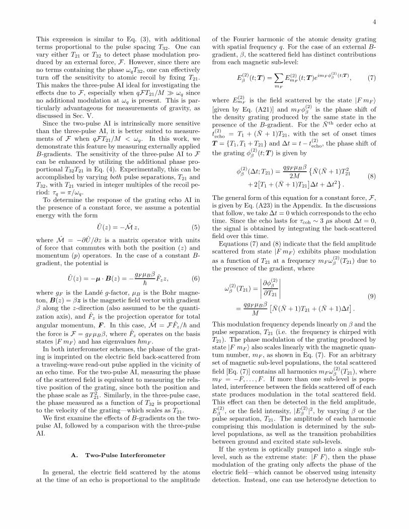
FIG. 1. (Color online) Recoil diagrams for the two-pulse (a)and three-pulse (b) AIs in the absence of any external forces.Standing wave excitations are labeled by SW1 – SW3. Att = T1 the atom is diffracted into a superposition of momen-tum states differing by integer (n) multiples of ~q. A secondsw pulse is applied at t = T2 which further diffracts the atoms.In the two-pulse case, interference between states differing by

~q (∆n = ±1) occurs at times t(2)echo = T1+(N+1)T21. For the

three-pulse scheme, a third sw pulse is applied at t = T3 which

produces interference at times t(3)echo = T1 + (N + 1)T21 + T32.

Examples of interfering trajectories for N = 1 and 2 are la-beled by solid black and dashed blue lines, respectively. Cir-cles indicate locations where interference fringes occur withspatial frequency q.

2

dicate that this AI is particularly well-suited for precisemeasurements of the gravitational acceleration, g.We begin with a review of the two AI configurations

used in this work, which are illustrated in Fig. 1. Thetwo-pulse echo AI [12, 13, 16, 17] utilizes short (Raman-Nath) standing wave (sw) pulses to diffract a sampleof laser cooled atoms at t = T1 into a superpositionof momentum states: |n~q〉. Here, n is an integer andq = k1 − k2 ≈ 2k is the difference between the travelingwave vectors comprising the sw. At t = T2, a second swpulse further diffracts the atomic wave packets—creatingsets of center-of-mass trajectories that overlap and pro-duce interference in the form of a density modulation in

the vicinity of t(2)echo = T1+(N+1)T21, where T21 ≡ T2−T1

and N = 1, 2, . . . is the order of the echo, as shown inFig. 1(a). The induced density modulation is coherent forτcoh = 2/qσv ∼ 3 µs about these “echo” times, beyondwhich the modulation dephases due to the distribution ofvelocities in the sample. Here, σv = (2kBT /M)1/2 char-acterizes the width of the velocity distribution along z.A traveling wave pulse is applied along the z-direction

in the vicinity of t(2)echo to “read out” the amplitude of

the grating by coherently Bragg scattering light alongthe −z-direction. The duration of this signal is limitedby the coherence time, τcoh. Due to the nature of Braggdiffraction, this back-scattered light is proportional to theFourier component of the density distribution with spa-tial frequency q. This harmonic is only produced by inter-ference of momentum states that differ by ~q (∆n = ±1).As a result, the two-pulse AI exhibits a temporal modu-lation at the atomic recoil frequency, ωq = ~q2/2M , andis therefore sensitive to recoil effects.The three-pulse “stimulated” grating echo AI (hence-

forth referred to as the three-pulse AI) was first demon-strated in Ref. 13 using a single hyperfine ground state,and was termed a “stimulated” echo due to similari-ties in pulse geometry with the stimulated photon echoscheme [18–21]. Recent work involving this interferom-eter [15] has shown certain advantages over the two-pulse scheme for phase measurements of the atomic grat-ing. The three-pulse AI involves applying two sw pulsesat t = T1 and t = T2, followed by a third pulse ap-plied at t = T3 = T2 + T32, where T32 ≡ T3 − T2.This pulse geometry produces an echo in the vicinity of

t(3)echo = T1 + (N + 1)T21 + T32, as shown in Fig. 1(b).However, unlike the two-pulse AI where all pairs of tra-jectories produced by the second pulse interfere at theecho times, for the three-pulse AI only momentum statesof the same order (∆n = 0) after the second pulse pro-duce interference at the echo times for arbitrary T21 andT32. For this reason, the signal produced by this interfer-ometer as a function of T32 (with T21 fixed) is insensitiveto atomic recoil effects (i.e. no temporal modulation) andis therefore ideal for probing other effects—such as thosedue to a constant force on the atoms.Reference 22 extensively reviews the grating echo AI

and discusses applications relating to atomic recoil [16,17, 23–26], gravity and magnetic gradients [27].

Previous experiments based on this AI [12, 13, 16, 17,23–25, 28] were typically limited to T21 < 10 ms by de-coherence effects due to spatially and temporally varyingB-fields. Additionally, the sample temperature (typically∼ 50 µK) and excitation beam configuration (fixed fre-quency sw with ∼ 0.5 cm diameter) limited the transittime in these experiments. In this work, we have im-proved the level of B-field and B-gradient suppressionby using a non-magnetic vacuum chamber, which hasenabled the extension of AI signal lifetimes. The mag-netically controlled environment allows a sample of 85Rbatoms to be cooled to temperatures as low as 2.4 µK. Byexpanding the excitation beam diameter to ∼ 2 cm, andchirping the sw pulses to cancel Doppler shifts, echo AIsignal lifetimes of ∼ 220 ms and transit times of ∼ 270ms have been achieved. These timescales are comparableto those of fountain experiments involving Raman AIs[1, 2, 29]. In contrast, long-lived echo AI signals havebeen observed only by using magnetic guides to limittransverse cloud expansion [15].

The experimental apparatus presented here has madeit possible to exploit the aforementioned advantages ofthe echo AI for a variety of precision measurements, suchas the atomic recoil frequency [26] and the gravitationalacceleration [22], that are currently underway. Addi-tionally, we recently utilized this apparatus to performa coherent transient experiment with cold Rb atoms toachieve a precise determination of the atomic g-factorratio [30].

In this Article, we apply long timescales to understand-ing and detecting the effects of B-gradients using thetwo-pulse grating echo AI, as well as a three-pulse “stim-ulated” grating echo AI [13, 15]. The passive detectionof magnetic anomalies is of interest for various applica-tions, such as submarine and mine detection where theambient magnetic noise of the environment is large com-pared to the sensitivity of the instrument [31]. The influ-ence of gravity and B-gradients on AI experiments hasbeen considered in the past. Reference 32 calculates howsuch forces affect the visibility of interference patterns inatomic diffraction experiments. In previous work [27], wedemonstrated the effect of both gravity and B-gradientson the two-pulse AI. A theoretical description of theseeffects based on a spin-1/2 system was able to explainthe basic signal dependence on the pulse separation, T21,but was insufficient to model experimental data.

This work relies on an improved theoretical descriptionof a generalized echo AI that includes an arbitrary num-ber of sw excitation pulses, the effects of a constant forceon the atoms, spontaneous emission and the sub-levelstructure of the atomic ground state (the 5S1/2 F = 3

state of 85Rb is used in the experiment). Coupled withthese theoretical predictions, we achieve sensitivity tochanges in B-gradients at the level of ∼ 0.04 mG/cm. Inaddition, absolute measurements of B-gradients as smallas ∼ 0.3 mG/cm, and sensitivity to the curvature of B-fields are demonstrated. These results are consistent withindependent measurements of the spatial variation in the

3

B-field using a flux-gate magnetometer. These studieshelp place limits on the sensitivity of a broad class oftime-domain AIs to B-gradients.We also consider implications for achieving precise

measurements of g using the two- and three-pulse echoAIs. In particular, analysis of the three-pulse AI suggeststhere are significant advantages for measuring g over thetwo-pulse AI. Although the experimental apparatus usedin this work is not designed to detect gravitational effects,predictions of the grating phase modulation due to grav-ity for both AIs have been validated by measuring theeffects of externally applied B-gradients. Measurementsof g using these AIs will be presented elsewhere.This Article is organized as follows. In Sec. II we

present theoretical predictions for the two- and three-pulse AI signals in the presence of a homogeneous B-gradient. In Sec. III, we describe details related to theexperimental apparatus. We present the results of exper-iments related to long timescales in Sec. IV, and discussmeasurements of B-gradients using both the two-pulseand three-pulse techniques. Section V discusses the fea-sibility of a precise measurement of g using the formal-ism developed to describe B-gradients. We conclude inSec. VI. The Appendix presents a calculation of the sig-nal generated by a generalized echo AI—encompassingthe two- and three-pulse AIs—in the presence of a con-stant force.

II. THEORY

In this section, we present the key results of calcula-tions for both the two- and three-pulse AI signals in thepresence of a homogeneous B-gradient. Details of thecalculations—which are sufficiently general to account forany constant force on the atoms, and an arbitrary num-ber of excitation pulses—are presented in the Appendix.In general, the sensitivity of these interferometers can

be characterized by the space-time area they enclose.Since only those states differing by ~q at the echo timecontribute to the signal, the area of both AIs is primarilycontrolled by T21. In the absence of any external forces,the areas of the two- and three-pulse AIs can be calcu-lated by inspecting their recoil diagrams [Figs. 1(a) and1(b), respectively]

A(2) =~q

2MN(N + 1)

(

T(2)21

)2

, (1a)

A(3) =~q

2M

[

N(N + 1)(

T(3)21

)2

+ 2NT32T(3)21

]

, (1b)

where M is the mass of the atom. Henceforth, quan-tities containing superscripts (2) or (3) indicate the in-terferometer for which that quantity applies. At firstglance, it might appear that the three-pulse AI enclosesa larger area than the two-pulse AI due to the extraterm in Eq. (1b). However, one must compare the en-closed areas at the same echo times, which are given by

t(2)echo = T1+(N+1)T

(2)21 and t

(3)echo = T1+(N+1)T

(3)21 +T32

for the two- and three-pulse schemes, respectively. By

setting t(2)echo = t

(3)echo, it can be shown that A(2) −A(3) =

~qNT 232/2M(N+1). This suggests that the two-pulse AI

is always more sensitive to external forces than the three-pulse AI. Nevertheless, the three-pulse AI offers a uniquefeature: the spatial separation between interfering wavepackets remains constant between the application of thesecond and third sw pulses. This is advantageous becauselarger spatial separations leads to increased decoherence,and therefore reduced timescale in the experiment [15].Since the separation can be precisely controlled by thepulse separation T21, one can increase the signal lifetimeby using smaller T21.Additionally, since the signal generated by the two-

pulse AI is modulated at the recoil frequency, ωq, thereare periodic regions where the signal-to-noise ratio is lessthan one and not well-suited for accurate phase measure-ments. However, the three-pulse technique is insensitiveto atomic recoil if T21 is fixed. Therefore, the scatteredfield amplitude has no additional modulation at ωq as T32

is varied—allowing regions of low signal-to-noise ratio tobe avoided.Both the gravitational force and a constant B-gradient

produce a constant force on the atoms, F = F z, whichgenerates a phase shift in the atomic interference pattern.The basic physical mechanism that produces this phaseshift is a difference in potential energy between the twoarms of the AI. One can compute the relative phase be-tween the two arms ∆φ = (SB−SA)/~ using the classicalaction [3]

S(t) =∫ t

0

L[z(t′), z(t′)]dt′, (2)

where L = Mz2/2 + Fz is the Lagrangian in this case.If SB and SA represent, respectively, the action alongthe upper and lower arms of the two-pulse AI, it can beshown that the phase shift between these arms is

∆φ(2) = N(N + 1)

[

ωqT21 +qFM

T 221

]

+ N2qv0T21, (3)

where v0 is the initial velocity of the atom along thez-direction. The term proportional to v0 is due to therelative Doppler shift between the two arms of the AI.Since the atomic sample has a finite velocity distribution(characterized by a 1/e radius, σv, and temperature, T ),this term is responsible for the coherence time of the echo:τcoh = 2/qσv. As expected, the contribution to the phaseshift from the potential energy (the term proportional toF) is independent of the initial velocity of the cloud.A similar calculation for the relative phase shift be-

tween the arms of the three-pulse AI yields

∆φ(3) = N(N + 1)

[

ωqT21 +qFM

T 221

]

+ NqFM

T32T21 + Nqv0(T32 + NT21).

(4)

4

This expression is similar to Eq. (3), with additionalterms proportional to the pulse spacing T32. One canvary either T21 or T32 to detect phase modulation pro-duced by an external force, F . However, since there areno terms containing the phase ωqT32, one can effectivelyturn off the sensitivity to atomic recoil by fixing T21.This makes the three-pulse AI ideal for investigating theeffects due to F , especially when qFT21/M ≫ ωq sinceno additional modulation at ωq is present. This is par-ticularly advantageous for measurements of gravity, asdiscussed in Sec. V.Since the two-pulse AI is intrinsically more sensitive

than the three-pulse AI, it is better suited to measure-ments of F when qFT21/M < ωq. In this work, wedemonstrate this feature by measuring externally appliedB-gradients. The sensitivity of the three-pulse AI to Fcan be enhanced by utilizing the additional phase pro-portional T32T21 in Eq. (4). Experimentally, this can beaccomplished by varying both pulse separations, T21 andT32, with T21 varied in integer multiples of the recoil pe-riod: τq = π/ωq.To determine the response of the grating echo AI in

the presence of a constant force, we assume a potentialenergy with the form

U(z) = −M z, (5)

where M = −∂U/∂z is a matrix operator with unitsof force that commutes with both the position (z) andmomentum (p) operators. In the case of a constant B-gradient, the potential is

U(z) = −µ ·B(z) = −gFµBβ

~Fzz, (6)

where gF is the Lande g-factor, µB is the Bohr magne-ton, B(z) = βz is the magnetic field vector with gradientβ along the z-direction (also assumed to be the quanti-

zation axis), and Fz is the projection operator for total

angular momentum, F . In this case, M = F Fz/~ and

the force is F = gFµBβ, where Fz operates on the basisstates |F mF 〉 and has eigenvalues ~mF .In both interferometer schemes, the phase of the grat-

ing is imprinted on the electric field back-scattered froma traveling-wave read-out pulse applied in the vicinity ofan echo time. For the two-pulse AI, measuring the phaseof the scattered field is equivalent to measuring the rela-tive position of the grating, since both the position andthe phase scale as T 2

21. Similarly, in the three-pulse case,the phase measured as a function of T32 is proportionalto the velocity of the grating—which scales as T21.We first examine the effects of B-gradients on the two-

pulse AI, followed by a comparison with the three-pulseAI.

A. Two-Pulse Interferometer

In general, the electric field scattered by the atomsat the time of an echo is proportional to the amplitude

of the Fourier harmonic of the atomic density gratingwith spatial frequency q. For the case of an external B-gradient, β, the scattered field has distinct contributionsfrom each magnetic sub-level:

E(2)β (t;T ) =

∑

mF

E(2)mF

(t;T )eimF φ(2)β

(t;T ), (7)

where E(2)mF is the field scattered by the state |F mF 〉

[given by Eq. (A21)] and mFφ(2)β is the phase shift of

the density grating produced by the same state in thepresence of the B-gradient. For the N th order echo at

t(2)echo = T1 + (N + 1)T21, with the set of onset times

T = T1, T1 + T21 and ∆t = t− t(2)echo, the phase shift of

the grating φ(2)β (t;T ) is given by

φ(2)β (∆t;T21) =

qgFµBβ

2M

N(N + 1)T 221

+2[

T1 + (N + 1)T21

]

∆t+∆t2

.(8)

The general form of this equation for a constant force, F ,is given by Eq. (A23) in the Appendix. In the discussionsthat follow, we take ∆t = 0 which corresponds to the echotime. Since the echo lasts for τcoh ∼ 3 µs about ∆t = 0,the signal is obtained by integrating the back-scatteredfield over this time.Equations (7) and (8) indicate that the field amplitude

scattered from state |F mF 〉 exhibits phase modulation

as a function of T21 at a frequency mFω(2)β (T21) due to

the presence of the gradient, where

ω(2)β (T21) =

∣

∣

∣

∣

∣

∂φ(2)β

∂T21

∣

∣

∣

∣

∣

=qgFµBβ

M

[

N(N + 1)T21 + (N + 1)∆t]

.

(9)

This modulation frequency depends linearly on β and thepulse separation, T21 (i.e. the frequency is chirped withT21). The phase modulation of the grating produced bystate |F mF 〉 also scales linearly with the magnetic quan-tum number, mF , as shown in Eq. (7). For an arbitraryset of magnetic sub-level populations, the total scattered

field [Eq. (7)] contains all harmonics mFω(2)β (T21), where

mF = −F, . . . , F . If more than one sub-level is popu-lated, interference between the fields scattered off of eachstate produces modulation in the total scattered field.This effect can then be detected in the field amplitude,

E(2)β , or the field intensity, |E(2)

β |2, by varying β or thepulse separation, T21. The amplitude of each harmoniccomprising this modulation is determined by the sub-level populations, as well as the transition probabilitiesbetween ground and excited state sub-levels.If the system is optically pumped into a single sub-

level, such as the extreme state: |F F 〉, then the phasemodulation of the grating only affects the phase of theelectric field—which cannot be observed using intensitydetection. Instead, one can use heterodyne detection to

5

HaL

0 5 10 15 20 25 30-1.0

-0.5

0.0

0.5

1.0

T21 HmsL

Re@

EΒH2L H

T21LDHa

rb.u

nitsL

HbL

0 2 4 6 8 10 12 14-1.0

-0.5

0.0

0.5

1.0

T21 HmsL

Re@

EΒH2L H

T21LDHa

rb.u

nitsL

HcL

0 20 40 60 80 100-1.0

-0.5

0.0

0.5

1.0

T32 HmsL

Re@

EΒH3L H

T32LDHa

rb.u

nitsL

HdL0 10 20 30 40 50

-1.0

-0.5

0.0

0.5

1.0

T32 HmsL

Re@

EΒH3L H

T32LDHa

rb.u

nitsL

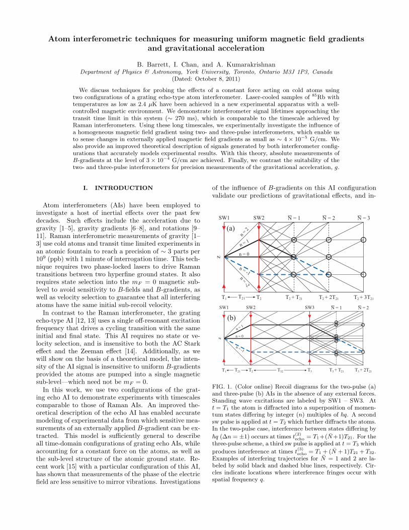
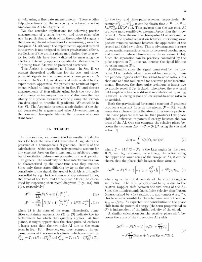
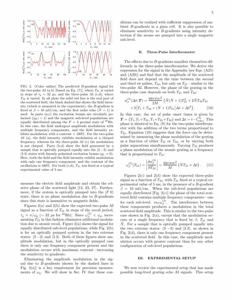
FIG. 2. (Color online) The predicted B-gradient signal forthe two-pulse AI (a,b) [based on Eq. (7)], where T21 is variedin steps of τq ∼ 32 µs, and the three-pulse AI (c,d), whereT32 is varied. In all plots the solid red line is the real part ofthe scattered field, the black dashed line shows the field inten-sity (which is measured in the experiment), the B-gradient isfixed at β = 10 mG/cm, and the first order echo (N = 1) isused. In parts (a,c) the excitation beams are circularly po-larized (|qL| = 1) and the magnetic sub-level populations areequally distributed among the F = 3 ground state of 85Rb.In this case, the field undergoes amplitude modulation withmultiple frequency components, and the field intensity ex-hibits modulation with a contrast < 100%. For the two-pulseAI (a), the field intensity exhibits modulation at a chirpedfrequency, whereas for the three-pulse AI (c) the modulationis not chirped. Parts (b,d) show the field generated by asample that is optically pumped equally into the |3 −3〉 and|3 3〉 states with linearly polarized excitation beams (qL = 0).Here, both the field and the field intensity exhibit modulationwith only one frequency component, and the contrast of theoscillations is 100%. For both (c,d), T21 was fixed at a typicalexperimental value of 5 ms.

measure the electric field amplitude and obtain the rel-ative phase of the scattered light [12, 23, 27]. Further-more, if the system is optically pumped into the |F 0〉state, there is no phase modulation due to B-gradientssince this state is insensitive to magnetic fields.

Figures 2(a) and 2(b) show the expected two-pulse AIsignal as a function of T21 in steps of the recoil period,

τq = π/ωq (∼ 32 µs for 85Rb). Since ω(2)β < ωq, incre-

menting T21 in this fashion eliminates additional modula-tion due to atomic recoil. Figure 2(a) shows the signal forequally distributed sub-level populations, while Fig. 2(b)is for an optically pumped system in the two extremestates: |3 −3〉 and |3 3〉. Both of these figures show am-plitude modulation, but in the optically pumped casethere is only one frequency component present and themodulation occurs with maximum contrast—increasingthe sensitivity to gradients.

Eliminating the amplitude modulation in the sig-nal due to B-gradients [shown by the dashed lines inFig. 2(a)] is a key requirement for precision measure-ments of ωq. We will show in Sec. IV that these con-

ditions can be realized with sufficient suppression of am-bient B-gradients in a glass cell. It is also possible toeliminate sensitivity to B-gradients using intensity de-tection if the atoms are pumped into a single magneticsub-level.

B. Three-Pulse Interferometer

The effects due to B-gradients manifest themselves dif-ferently in the three-pulse interferometer. We derive theexpression for the signal in the Appendix [see Eqs. (A25)and (A29)] and find that the amplitude of the scatteredfield does not depend on the time between the secondand third sw pulses, T32, but only on T21—similar to thetwo-pulse AI. However, the phase of the grating in thethree-pulse case depends on both T21 and T32:

φ(3)β (∆t;T ) =

qgFµBβ

2M

N(N + 1)T 221 + 2NT32T21

+2[

T1 + T32 + (N + 1)T21

]

∆t+∆t2

. (10)

In this case, the set of pulse onset times is given by

T = T1, T1+T21, T1+T21+T32 and ∆t = t−t(3)echo. This

phase is identical to Eq. (8) for the two-pulse interferom-eter with the addition of the two terms proportional toT32. Equation (10) suggests that the force can be deter-mined by measuring the phase modulation of the gratingas a function of either T21 or T32, or by varying bothpulse separations simultaneously. Varying T32 producesa phase modulation of the atomic grating at a frequencythat is proportional to T21:

ω(3)β (T21) =

∣

∣

∣

∣

∣

∂φ(3)β

∂T32

∣

∣

∣

∣

∣

=qgFµBβ

M

(

NT21 +∆t)

. (11)

Figures 2(c) and 2(d) show the expected three-pulsesignal as a function of T32, with T21 fixed at a typical ex-perimental value of 5 ms, in the presence of a B-gradientβ = 10 mG/cm. When the sub-level populations areequally distributed [Fig. 2(c)] the phase of the total scat-tered field contains multiple frequency components—one

for each sub-level: mFω(3)β . The interference between

these components produces a modulation in the totalscattered field amplitude. This is similar to the two-pulsecase shown in Fig. 2(a), except that the modulation oc-curs at a single frequency that is fixed by β, T21 andN . For a sample that is optically pumped equally intothe two extreme states: |3 −3〉 and |3 3〉, as shown inFig. 2(d), there is only one frequency component presentin the scattered field. In this case, the amplitude mod-ulation occurs with greater contrast than for any otherconfiguration of sub-level populations.

III. EXPERIMENTAL SETUP

We now review the experimental setup that has madepossible long-lived grating echo AI signals. This setup

6

is substantially different from previous echo experiments[16, 24, 25, 27] after implementing many improvements.These include suppression of stray magnetic gradientsusing a non-magnetic chamber, increasing the trappedatom number with large diameter beams, extending thetransit time by cooling the sample to ∼ 10 µK and imple-menting large diameter excitation beams, and by chirp-ing the excitation frequencies to eliminate Doppler shiftsassociated with the falling cloud.

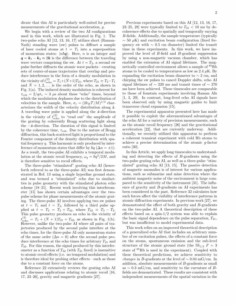
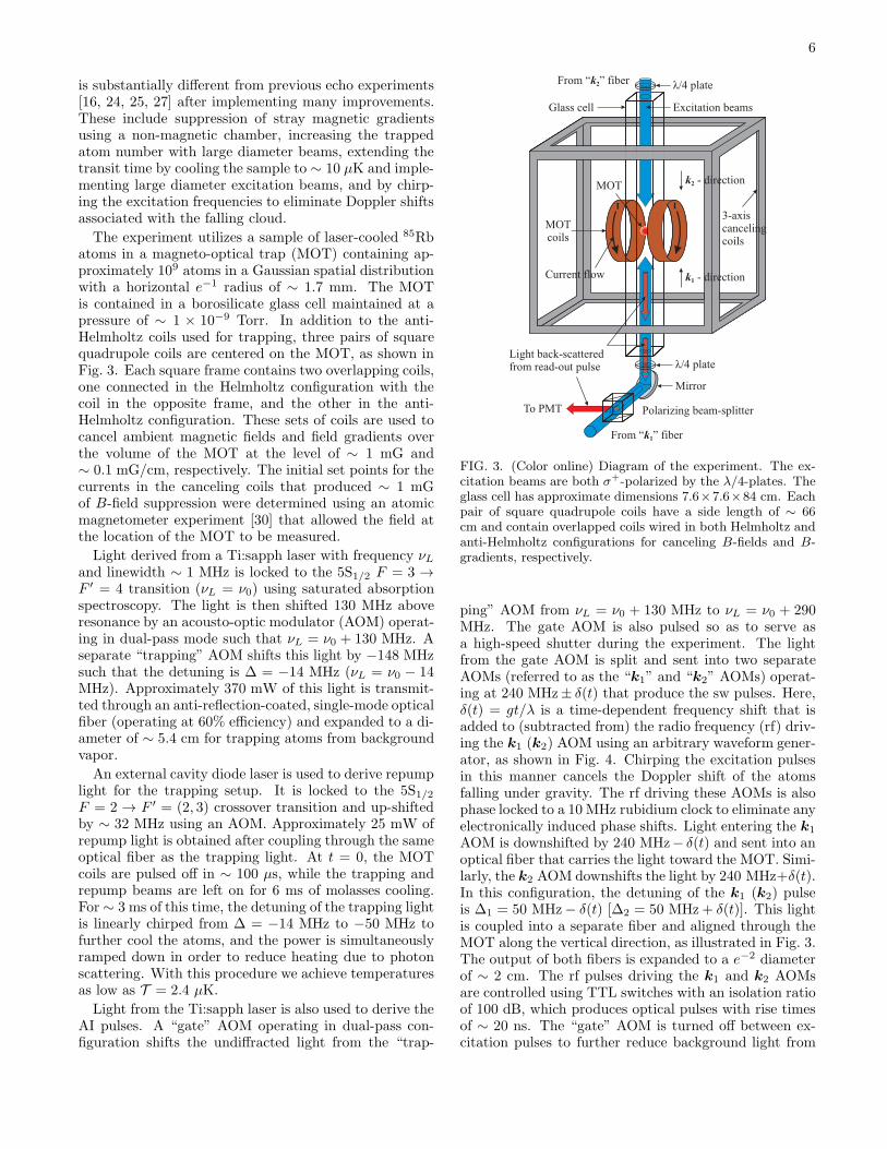
The experiment utilizes a sample of laser-cooled 85Rbatoms in a magneto-optical trap (MOT) containing ap-proximately 109 atoms in a Gaussian spatial distributionwith a horizontal e−1 radius of ∼ 1.7 mm. The MOTis contained in a borosilicate glass cell maintained at apressure of ∼ 1 × 10−9 Torr. In addition to the anti-Helmholtz coils used for trapping, three pairs of squarequadrupole coils are centered on the MOT, as shown inFig. 3. Each square frame contains two overlapping coils,one connected in the Helmholtz configuration with thecoil in the opposite frame, and the other in the anti-Helmholtz configuration. These sets of coils are used tocancel ambient magnetic fields and field gradients overthe volume of the MOT at the level of ∼ 1 mG and∼ 0.1 mG/cm, respectively. The initial set points for thecurrents in the canceling coils that produced ∼ 1 mGof B-field suppression were determined using an atomicmagnetometer experiment [30] that allowed the field atthe location of the MOT to be measured.

Light derived from a Ti:sapph laser with frequency νLand linewidth ∼ 1 MHz is locked to the 5S1/2 F = 3 →F ′ = 4 transition (νL = ν0) using saturated absorptionspectroscopy. The light is then shifted 130 MHz aboveresonance by an acousto-optic modulator (AOM) operat-ing in dual-pass mode such that νL = ν0 + 130 MHz. Aseparate “trapping” AOM shifts this light by −148 MHzsuch that the detuning is ∆ = −14 MHz (νL = ν0 − 14MHz). Approximately 370 mW of this light is transmit-ted through an anti-reflection-coated, single-mode opticalfiber (operating at 60% efficiency) and expanded to a di-ameter of ∼ 5.4 cm for trapping atoms from backgroundvapor.

An external cavity diode laser is used to derive repumplight for the trapping setup. It is locked to the 5S1/2F = 2 → F ′ = (2, 3) crossover transition and up-shiftedby ∼ 32 MHz using an AOM. Approximately 25 mW ofrepump light is obtained after coupling through the sameoptical fiber as the trapping light. At t = 0, the MOTcoils are pulsed off in ∼ 100 µs, while the trapping andrepump beams are left on for 6 ms of molasses cooling.For ∼ 3 ms of this time, the detuning of the trapping lightis linearly chirped from ∆ = −14 MHz to −50 MHz tofurther cool the atoms, and the power is simultaneouslyramped down in order to reduce heating due to photonscattering. With this procedure we achieve temperaturesas low as T = 2.4 µK.

Light from the Ti:sapph laser is also used to derive theAI pulses. A “gate” AOM operating in dual-pass con-figuration shifts the undiffracted light from the “trap-

FIG. 3. (Color online) Diagram of the experiment. The ex-citation beams are both σ+-polarized by the λ/4-plates. Theglass cell has approximate dimensions 7.6×7.6×84 cm. Eachpair of square quadrupole coils have a side length of ∼ 66cm and contain overlapped coils wired in both Helmholtz andanti-Helmholtz configurations for canceling B-fields and B-gradients, respectively.

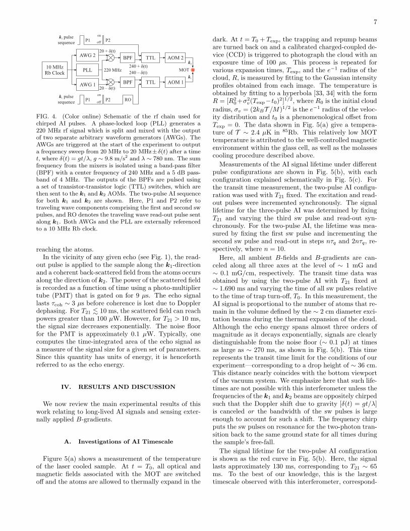
ping” AOM from νL = ν0 + 130 MHz to νL = ν0 + 290MHz. The gate AOM is also pulsed so as to serve asa high-speed shutter during the experiment. The lightfrom the gate AOM is split and sent into two separateAOMs (referred to as the “k1” and “k2” AOMs) operat-ing at 240 MHz± δ(t) that produce the sw pulses. Here,δ(t) = gt/λ is a time-dependent frequency shift that isadded to (subtracted from) the radio frequency (rf) driv-ing the k1 (k2) AOM using an arbitrary waveform gener-ator, as shown in Fig. 4. Chirping the excitation pulsesin this manner cancels the Doppler shift of the atomsfalling under gravity. The rf driving these AOMs is alsophase locked to a 10 MHz rubidium clock to eliminate anyelectronically induced phase shifts. Light entering the k1

AOM is downshifted by 240 MHz− δ(t) and sent into anoptical fiber that carries the light toward the MOT. Simi-larly, the k2 AOM downshifts the light by 240 MHz+δ(t).In this configuration, the detuning of the k1 (k2) pulseis ∆1 = 50 MHz− δ(t) [∆2 = 50 MHz + δ(t)]. This lightis coupled into a separate fiber and aligned through theMOT along the vertical direction, as illustrated in Fig. 3.The output of both fibers is expanded to a e−2 diameterof ∼ 2 cm. The rf pulses driving the k1 and k2 AOMsare controlled using TTL switches with an isolation ratioof 100 dB, which produces optical pulses with rise timesof ∼ 20 ns. The “gate” AOM is turned off between ex-citation pulses to further reduce background light from

7

FIG. 4. (Color online) Schematic of the rf chain used forchirped AI pulses. A phase-locked loop (PLL) generates a220 MHz rf signal which is split and mixed with the outputof two separate arbitrary waveform generators (AWGs). TheAWGs are triggered at the start of the experiment to outputa frequency sweep from 20 MHz to 20 MHz±δ(t) after a timet, where δ(t) = gt/λ, g ∼ 9.8 m/s2 and λ ∼ 780 nm. The sumfrequency from the mixers is isolated using a band-pass filter(BPF) with a center frequency of 240 MHz and a 5 dB pass-band of 4 MHz. The outputs of the BPFs are pulsed usinga set of transistor-transistor logic (TTL) switches, which arethen sent to the k1 and k2 AOMs. The two-pulse AI sequencefor both k1 and k2 are shown. Here, P1 and P2 refer totraveling wave components comprising the first and second swpulses, and RO denotes the traveling wave read-out pulse sentalong k1. Both AWGs and the PLL are externally referencedto a 10 MHz Rb clock.

reaching the atoms.In the vicinity of any given echo (see Fig. 1), the read-

out pulse is applied to the sample along the k1-directionand a coherent back-scattered field from the atoms occursalong the direction of k2. The power of the scattered fieldis recorded as a function of time using a photo-multipliertube (PMT) that is gated on for 9 µs. The echo signallasts τcoh ∼ 3 µs before coherence is lost due to Dopplerdephasing. For T21 . 10 ms, the scattered field can reachpowers greater than 100 µW. However, for T21 > 10 ms,the signal size decreases exponentially. The noise floorfor the PMT is approximately 0.1 µW. Typically, onecomputes the time-integrated area of the echo signal asa measure of the signal size for a given set of parameters.Since this quantity has units of energy, it is henceforthreferred to as the echo energy.

IV. RESULTS AND DISCUSSION

We now review the main experimental results of thiswork relating to long-lived AI signals and sensing exter-nally applied B-gradients.

A. Investigations of AI Timescale

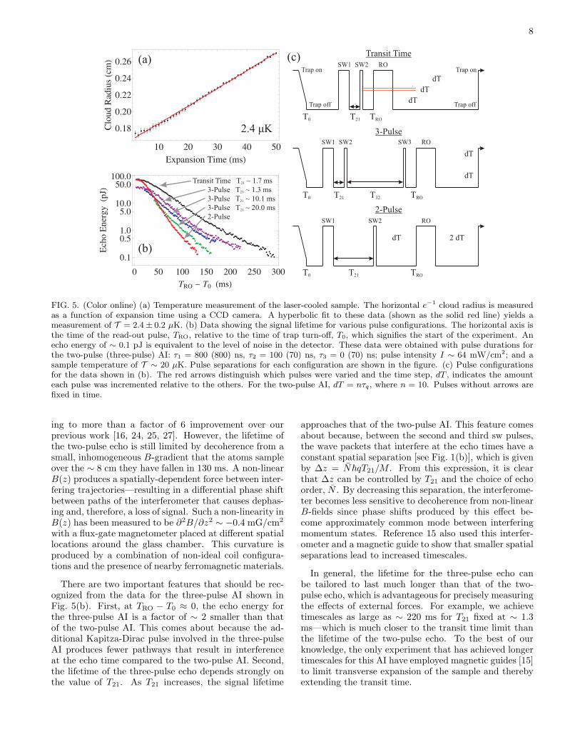
Figure 5(a) shows a measurement of the temperatureof the laser cooled sample. At t = T0, all optical andmagnetic fields associated with the MOT are switchedoff and the atoms are allowed to thermally expand in the

dark. At t = T0 + Texp, the trapping and repump beamsare turned back on and a calibrated charged-coupled de-vice (CCD) is triggered to photograph the cloud with anexposure time of 100 µs. This process is repeated forvarious expansion times, Texp, and the e−1 radius of thecloud, R, is measured by fitting to the Gaussian intensityprofiles obtained from each image. The temperature isobtained by fitting to a hyperbola [33, 34] with the formR = [R2

0+σ2v(Texp−t0)

2]1/2, where R0 is the initial cloud

radius, σv = (2kBT /M)1/2 is the e−1 radius of the veloc-ity distribution and t0 is a phenomenological offset fromTexp = 0. The data shown in Fig. 5(a) give a tempera-ture of T ∼ 2.4 µK in 85Rb. This relatively low MOTtemperature is attributed to the well-controlled magneticenvironment within the glass cell, as well as the molassescooling procedure described above.

Measurements of the AI signal lifetime under differentpulse configurations are shown in Fig. 5(b), with eachconfiguration explained schematically in Fig. 5(c). Forthe transit time measurement, the two-pulse AI configu-ration was used with T21 fixed. The excitation and read-out pulses were incremented synchronously. The signallifetime for the three-pulse AI was determined by fixingT21 and varying the third sw pulse and read-out syn-chronously. For the two-pulse AI, the lifetime was mea-sured by fixing the first sw pulse and incrementing thesecond sw pulse and read-out in steps nτq and 2nτq, re-spectively, where n = 10.

Here, all ambient B-fields and B-gradients are can-celed along all three axes at the level of ∼ 1 mG and∼ 0.1 mG/cm, respectively. The transit time data wasobtained by using the two-pulse AI with T21 fixed at∼ 1.690 ms and varying the time of all sw pulses relativeto the time of trap turn-off, T0. In this measurement, theAI signal is proportional to the number of atoms that re-main in the volume defined by the ∼ 2 cm diameter exci-tation beams during the thermal expansion of the cloud.Although the echo energy spans almost three orders ofmagnitude as it decays exponentially, signals are clearlydistinguishable from the noise floor (∼ 0.1 pJ) at timesas large as ∼ 270 ms, as shown in Fig. 5(b). This timerepresents the transit time limit for the conditions of ourexperiment—corresponding to a drop height of ∼ 36 cm.This distance nearly coincides with the bottom viewportof the vacuum system. We emphasize here that such life-times are not possible with this interferometer unless thefrequencies of the k1 and k2 beams are oppositely chirpedsuch that the Doppler shift due to gravity [δ(t) = gt/λ]is canceled or the bandwidth of the sw pulses is largeenough to account for such a shift. The frequency chirpputs the sw pulses on resonance for the two-photon tran-sition back to the same ground state for all times duringthe sample’s free-fall.

The signal lifetime for the two-pulse AI configurationis shown as the red curve in Fig. 5(b). Here, the signallasts approximately 130 ms, corresponding to T21 ∼ 65ms. To the best of our knowledge, this is the largesttimescale observed with this interferometer, correspond-

8

FIG. 5. (Color online) (a) Temperature measurement of the laser-cooled sample. The horizontal e−1 cloud radius is measuredas a function of expansion time using a CCD camera. A hyperbolic fit to these data (shown as the solid red line) yields ameasurement of T = 2.4± 0.2 µK. (b) Data showing the signal lifetime for various pulse configurations. The horizontal axis isthe time of the read-out pulse, TRO, relative to the time of trap turn-off, T0, which signifies the start of the experiment. Anecho energy of ∼ 0.1 pJ is equivalent to the level of noise in the detector. These data were obtained with pulse durations forthe two-pulse (three-pulse) AI: τ1 = 800 (800) ns, τ2 = 100 (70) ns, τ3 = 0 (70) ns; pulse intensity I ∼ 64 mW/cm2; and asample temperature of T ∼ 20 µK. Pulse separations for each configuration are shown in the figure. (c) Pulse configurationsfor the data shown in (b). The red arrows distinguish which pulses were varied and the time step, dT , indicates the amounteach pulse was incremented relative to the others. For the two-pulse AI, dT = nτq , where n = 10. Pulses without arrows arefixed in time.

ing to more than a factor of 6 improvement over ourprevious work [16, 24, 25, 27]. However, the lifetime ofthe two-pulse echo is still limited by decoherence from asmall, inhomogeneous B-gradient that the atoms sampleover the ∼ 8 cm they have fallen in 130 ms. A non-linearB(z) produces a spatially-dependent force between inter-fering trajectories—resulting in a differential phase shiftbetween paths of the interferometer that causes dephas-ing and, therefore, a loss of signal. Such a non-linearity inB(z) has been measured to be ∂2B/∂z2 ∼ −0.4 mG/cm2

with a flux-gate magnetometer placed at different spatiallocations around the glass chamber. This curvature isproduced by a combination of non-ideal coil configura-tions and the presence of nearby ferromagnetic materials.

There are two important features that should be rec-ognized from the data for the three-pulse AI shown inFig. 5(b). First, at TRO − T0 ≈ 0, the echo energy forthe three-pulse AI is a factor of ∼ 2 smaller than thatof the two-pulse AI. This comes about because the ad-ditional Kapitza-Dirac pulse involved in the three-pulseAI produces fewer pathways that result in interferenceat the echo time compared to the two-pulse AI. Second,the lifetime of the three-pulse echo depends strongly onthe value of T21. As T21 increases, the signal lifetime

approaches that of the two-pulse AI. This feature comesabout because, between the second and third sw pulses,the wave packets that interfere at the echo times have aconstant spatial separation [see Fig. 1(b)], which is givenby ∆z = N~qT21/M . From this expression, it is clearthat ∆z can be controlled by T21 and the choice of echoorder, N . By decreasing this separation, the interferome-ter becomes less sensitive to decoherence from non-linearB-fields since phase shifts produced by this effect be-come approximately common mode between interferingmomentum states. Reference 15 also used this interfer-ometer and a magnetic guide to show that smaller spatialseparations lead to increased timescales.

In general, the lifetime for the three-pulse echo canbe tailored to last much longer than that of the two-pulse echo, which is advantageous for precisely measuringthe effects of external forces. For example, we achievetimescales as large as ∼ 220 ms for T21 fixed at ∼ 1.3ms—which is much closer to the transit time limit thanthe lifetime of the two-pulse echo. To the best of ourknowledge, the only experiment that has achieved longertimescales for this AI have employed magnetic guides [15]to limit transverse expansion of the sample and therebyextending the transit time.

9

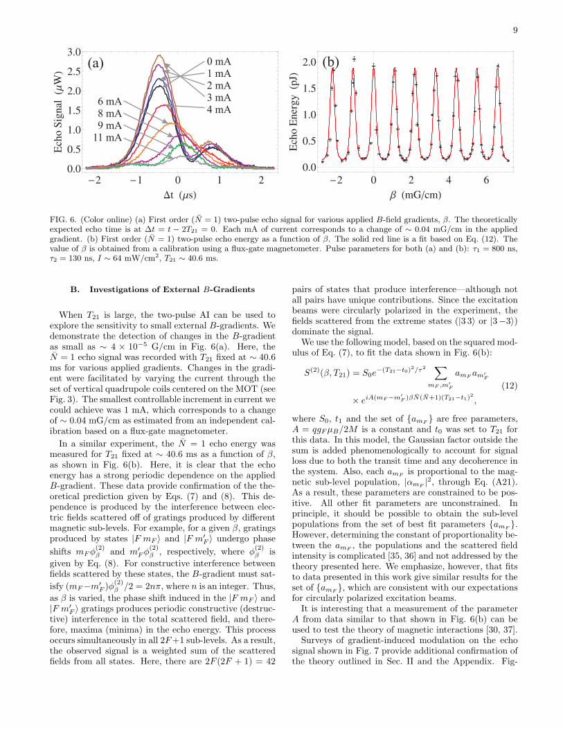
FIG. 6. (Color online) (a) First order (N = 1) two-pulse echo signal for various applied B-field gradients, β. The theoreticallyexpected echo time is at ∆t = t − 2T21 = 0. Each mA of current corresponds to a change of ∼ 0.04 mG/cm in the appliedgradient. (b) First order (N = 1) two-pulse echo energy as a function of β. The solid red line is a fit based on Eq. (12). Thevalue of β is obtained from a calibration using a flux-gate magnetometer. Pulse parameters for both (a) and (b): τ1 = 800 ns,τ2 = 130 ns, I ∼ 64 mW/cm2, T21 ∼ 40.6 ms.

B. Investigations of External B-Gradients

When T21 is large, the two-pulse AI can be used toexplore the sensitivity to small external B-gradients. Wedemonstrate the detection of changes in the B-gradientas small as ∼ 4 × 10−5 G/cm in Fig. 6(a). Here, theN = 1 echo signal was recorded with T21 fixed at ∼ 40.6ms for various applied gradients. Changes in the gradi-ent were facilitated by varying the current through theset of vertical quadrupole coils centered on the MOT (seeFig. 3). The smallest controllable increment in current wecould achieve was 1 mA, which corresponds to a changeof ∼ 0.04 mG/cm as estimated from an independent cal-ibration based on a flux-gate magnetometer.

In a similar experiment, the N = 1 echo energy wasmeasured for T21 fixed at ∼ 40.6 ms as a function of β,as shown in Fig. 6(b). Here, it is clear that the echoenergy has a strong periodic dependence on the appliedB-gradient. These data provide confirmation of the the-oretical prediction given by Eqs. (7) and (8). This de-pendence is produced by the interference between elec-tric fields scattered off of gratings produced by differentmagnetic sub-levels. For example, for a given β, gratingsproduced by states |F mF 〉 and |F m′

F 〉 undergo phase

shifts mFφ(2)β and m′

Fφ(2)β , respectively, where φ

(2)β is

given by Eq. (8). For constructive interference betweenfields scattered by these states, the B-gradient must sat-

isfy (mF−m′F )φ

(2)β /2 = 2nπ, where n is an integer. Thus,

as β is varied, the phase shift induced in the |F mF 〉 and|F m′

F 〉 gratings produces periodic constructive (destruc-tive) interference in the total scattered field, and there-fore, maxima (minima) in the echo energy. This processoccurs simultaneously in all 2F+1 sub-levels. As a result,the observed signal is a weighted sum of the scatteredfields from all states. Here, there are 2F (2F + 1) = 42

pairs of states that produce interference—although notall pairs have unique contributions. Since the excitationbeams were circularly polarized in the experiment, thefields scattered from the extreme states (|3 3〉 or |3−3〉)dominate the signal.We use the following model, based on the squared mod-

ulus of Eq. (7), to fit the data shown in Fig. 6(b):

S(2)(β, T21) = S0e−(T21−t0)

2/τ2 ∑

mF ,m′

F

amFam′

F

× eiA(mF−m′

F )βN(N+1)(T21−t1)2

,

(12)

where S0, t1 and the set of amF are free parameters,

A = qgFµB/2M is a constant and t0 was set to T21 forthis data. In this model, the Gaussian factor outside thesum is added phenomenologically to account for signalloss due to both the transit time and any decoherence inthe system. Also, each amF

is proportional to the mag-netic sub-level population, |αmF

|2, through Eq. (A21).As a result, these parameters are constrained to be pos-itive. All other fit parameters are unconstrained. Inprinciple, it should be possible to obtain the sub-levelpopulations from the set of best fit parameters amF

.However, determining the constant of proportionality be-tween the amF

, the populations and the scattered fieldintensity is complicated [35, 36] and not addressed by thetheory presented here. We emphasize, however, that fitsto data presented in this work give similar results for theset of amF

, which are consistent with our expectationsfor circularly polarized excitation beams.It is interesting that a measurement of the parameter

A from data similar to that shown in Fig. 6(b) can beused to test the theory of magnetic interactions [30, 37].Surveys of gradient-induced modulation on the echo

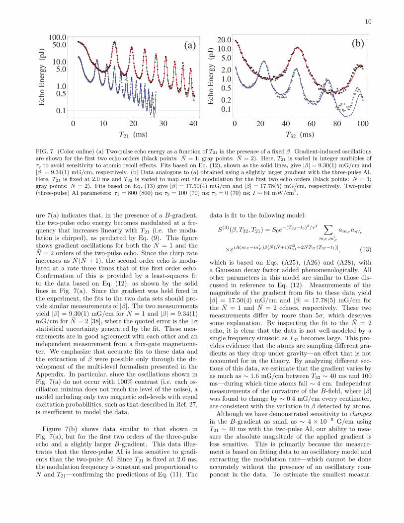
signal shown in Fig. 7 provide additional confirmation ofthe theory outlined in Sec. II and the Appendix. Fig-

10

FIG. 7. (Color online) (a) Two-pulse echo energy as a function of T21 in the presence of a fixed β. Gradient-induced oscillationsare shown for the first two echo orders (black points: N = 1; gray points: N = 2). Here, T21 is varied in integer multiples ofτq to avoid sensitivity to atomic recoil effects. Fits based on Eq. (12), shown as the solid lines, give |β| = 9.30(1) mG/cm and|β| = 9.34(1) mG/cm, respectively. (b) Data analogous to (a) obtained using a slightly larger gradient with the three-pulse AI.Here, T21 is fixed at 2.0 ms and T32 is varied to map out the modulation for the first two echo orders (black points: N = 1;gray points: N = 2). Fits based on Eq. (13) give |β| = 17.50(4) mG/cm and |β| = 17.78(5) mG/cm, respectively. Two-pulse(three-pulse) AI parameters: τ1 = 800 (800) ns; τ2 = 100 (70) ns; τ3 = 0 (70) ns; I ∼ 64 mW/cm2.

ure 7(a) indicates that, in the presence of a B-gradient,the two-pulse echo energy becomes modulated at a fre-quency that increases linearly with T21 (i.e. the modu-lation is chirped), as predicted by Eq. (9). This figureshows gradient oscillations for both the N = 1 and theN = 2 orders of the two-pulse echo. Since the chirp rateincreases as N(N + 1), the second order echo is modu-lated at a rate three times that of the first order echo.Confirmation of this is provided by a least-squares fitto the data based on Eq. (12), as shown by the solidlines in Fig. 7(a). Since the gradient was held fixed inthe experiment, the fits to the two data sets should pro-vide similar measurements of |β|. The two measurementsyield |β| = 9.30(1) mG/cm for N = 1 and |β| = 9.34(1)mG/cm for N = 2 [38], where the quoted error is the 1σstatistical uncertainty generated by the fit. These mea-surements are in good agreement with each other and anindependent measurement from a flux-gate magnetome-ter. We emphasize that accurate fits to these data andthe extraction of β were possible only through the de-velopment of the multi-level formalism presented in theAppendix. In particular, since the oscillations shown inFig. 7(a) do not occur with 100% contrast (i.e. each os-cillation minima does not reach the level of the noise), amodel including only two magnetic sub-levels with equalexcitation probabilities, such as that described in Ref. 27,is insufficient to model the data.

Figure 7(b) shows data similar to that shown inFig. 7(a), but for the first two orders of the three-pulseecho and a slightly larger B-gradient. This data illus-trates that the three-pulse AI is less sensitive to gradi-ents than the two-pulse AI. Since T21 is fixed at 2.0 ms,the modulation frequency is constant and proportional toN and T21—confirming the predictions of Eq. (11). The

data is fit to the following model:

S(3)(β, T32, T21) = S0e−(T32−t0)

2/τ2 ∑

mF ,m′

F

amFam′

F

×eiA(mF−m′

F )β[N(N+1)T 221+2NT21(T32−t1)], (13)

which is based on Eqs. (A25), (A26) and (A28), witha Gaussian decay factor added phenomenologically. Allother parameters in this model are similar to those dis-cussed in reference to Eq. (12). Measurements of themagnitude of the gradient from fits to these data yield|β| = 17.50(4) mG/cm and |β| = 17.78(5) mG/cm forthe N = 1 and N = 2 echoes, respectively. These twomeasurements differ by more than 5σ, which deservessome explanation. By inspecting the fit to the N = 2echo, it is clear that the data is not well-modeled by asingle frequency sinusoid as T32 becomes large. This pro-vides evidence that the atoms are sampling different gra-dients as they drop under gravity—an effect that is notaccounted for in the theory. By analyzing different sec-tions of this data, we estimate that the gradient varies byas much as ∼ 1.6 mG/cm between T32 ∼ 40 ms and 100ms—during which time atoms fall ∼ 4 cm. Independentmeasurements of the curvature of the B-field, where |β|was found to change by ∼ 0.4 mG/cm every centimeter,are consistent with the variation in β detected by atoms.Although we have demonstrated sensitivity to changes

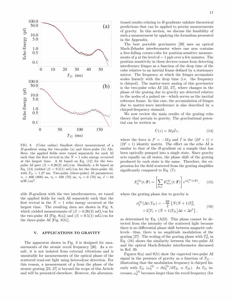
in the B-gradient as small as ∼ 4 × 10−5 G/cm usingT21 ∼ 40 ms with the two-pulse AI, our ability to mea-sure the absolute magnitude of the applied gradient isless sensitive. This is primarily because the measure-ment is based on fitting data to an oscillatory model andextracting the modulation rate—which cannot be doneaccurately without the presence of an oscillatory com-ponent in the data. To estimate the smallest measur-

11

FIG. 8. (Color online) Smallest direct measurement of aB-gradient using the two-pulse (a) and three-pulse (b) AIs.Here, the applied fields were tuned separately for each AIsuch that the first revival in the N = 1 echo energy occurredat the largest time. A fit based on Eq. (12) for the two-pulse AI gave |β| = 0.26(3) mG/cm. Similarly, a fit based onEq. (13) yielded |β| = 9.5(1) mG/cm for the three-pulse AI,with T21 ∼ 1.27 ms. Two-pulse (three-pulse) AI parameters:τ1 = 800 (800) ns, τ2 = 100 (70) ns, τ3 = 0 (70) ns, I ∼ 64mW/cm2.

able B-gradient with the two interferometers, we tunedthe applied fields for each AI separately such that thefirst revival in the N = 1 echo energy occurred at thelargest time. The resulting data are shown in Fig. 8,which yielded measurements of |β| = 0.26(3) mG/cm forthe two-pulse AI [Fig. 8(a)] and |β| = 9.5(1) mG/cm forthe three-pulse AI [Fig. 8(b)].

V. APPLICATIONS TO GRAVITY

The apparatus shown in Fig. 3 is designed for mea-surements of the atomic recoil frequency [26]. As a re-sult, it is not isolated from external vibrations and isunsuitable for measurements of the optical phase of thescattered read-out light using heterodyne detection. Forthis reason, a measurement of g from the phase of theatomic grating [22, 27] is beyond the scope of this Articleand will be presented elsewhere. However, the aforemen-

tioned results relating to B-gradients validate theoreticalpredictions that can be applied to precise measurementsof gravity. In this section, we discuss the feasibility ofsuch a measurement by applying the formalism presentedin the Appendix.The best portable gravimeter [39] uses an optical

Mach-Zehnder interferometer where one arm containsa free-falling corner-cube for position-sensitive measure-ments of g at the level of ∼ 1 ppb over a few minutes. Theposition sensitivity in these devices comes from detectinginterference fringes as a function of the drop time of thecube relative to an inertial frame defined by a stationarymirror. The frequency at which the fringes accumulatescales linearly with the drop time (i.e. the frequencyis chirped). The matter-wave analog of this gravimeteris the two-pulse echo AI [22, 27], where changes in thephase of the grating due to gravity are detected relativeto the nodes of a pulsed sw—which serves as the inertialreference frame. In this case, the accumulation of fringesdue to matter-wave interference is also described by achirped-frequency sinusoid.We now review the main results of the grating echo

theory that pertain to gravity. The gravitational poten-tial can be written as

U(z) = MgIz, (14)

where the force is F = −Mg and I is the (2F + 1) ×(2F + 1) identity matrix. The effect on the echo AI issimilar to that of the B-gradient on a sample that hasbeen optically pumped into a single state. Since gravityacts equally on all states, the phase shift of the gratingproduced by each state is the same. Therefore, the ex-pression for the field scattered from the grating simplifiessignificantly compared to Eq. (7):

E(2)g (t;T ) =

[

∑

mF

E(2)mF

(t;T )

]

eiφ(2)g (t;T ), (15)

where the grating phase due to gravity is

φ(2)g (∆t;T21) = −qg

2

N(N + 1)T 221

+2[

T1 + (N + 1)T21

]

∆t+∆t2

,(16)

as determined by Eq. (A23). This phase cannot be de-tected from the intensity of the scattered light becausethere is no differential phase shift between magnetic sub-levels—thus, there is no amplitude modulation of thegrating [27]. The scaling of the grating phase with T 2

21 inEq. (16) shows the similarity between the two-pulse AIand the optical Mach-Zehnder interferometer discussedin Ref. 39.Figures 9(a) and 9(b) show the expected two-pulse AI

signal in the presence of gravity as a function of T21—illustrating that the modulation frequency is chirped lin-

early with T21 (ω(2)g = ∂φ

(2)g /∂T21 ∝ T21). As T21 in-

creases, ω(2)g becomes larger than the recoil frequency (for

12

HaL

0.97 0.98 0.99 1.00 1.01 1.02 1.03-1.0

-0.5

0.0

0.5

1.0

T21 HmsL

Re@

EgH2L H

T21LDHa

rb.u

nitsL

HbL

8.97 8.98 8.99 9.00 9.01 9.02 9.03-1.0

-0.5

0.0

0.5

1.0

T21 HmsL

Re@

EgH2L H

T21LDHa

rb.u

nitsL

HcL

0.97 0.98 0.99 1.00 1.01 1.02 1.03-1.0

-0.5

0.0

0.5

1.0

T21 HmsL

Re@

EgH3L H

T21LDHa

rb.u

nitsL

HdL

8.97 8.98 8.99 9.00 9.01 9.02 9.03-1.0

-0.5

0.0

0.5

1.0

T21 HmsL

Re@

EgH3L H

T21LDHa

rb.u

nitsL

HeL

0.97 0.98 0.99 1.00 1.01 1.02 1.03-1.0

-0.5

0.0

0.5

1.0

T32 HmsL

Re@

EgH3L H

T32LDHa

rb.u

nitsL

Hf L

8.97 8.98 8.99 9.00 9.01 9.02 9.03-1.0

-0.5

0.0

0.5

1.0

T32 HmsL

Re@

EgH3L H

T32LDHa

rb.u

nitsL

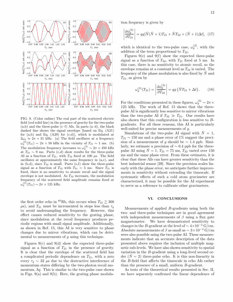
FIG. 9. (Color online) The real part of the scattered electricfield (red solid line) in the presence of gravity for the two-pulse(a,b) and the three-pulse (c–f) AIs. In parts (a–d), the blackdashed line shows the signal envelope [based on Eq. (A21)for (a,b) and Eq. (A29) for (c,d)], which is modulated at2ωq ≈ 2π × 31 kHz. (a) The field oscillates at a frequency

ω(2)g (T21) ∼ 2π × 50 kHz in the vicinity of T21 ∼ 1 ms. (b)

The modulation frequency increases to ω(2)g ∼ 2π × 450 kHz

at T21 ∼ 9 ms. Parts (c,d) show results for the three-pulseAI as a function of T21, with T32 fixed at 100 µs. The fieldoscillates at approximately the same frequency in (a,c), andin (b,d), since T32 is small. Parts (e,f) show the three-pulsesignal as a function of T32 with T21 = 5 ms. Since T21 isfixed, there is no sensitivity to atomic recoil and the signalenvelope is not modulated. As T32 increases, the modulationfrequency of the scattered field amplitude remains fixed at

ω(3)g (T21) ∼ 2π × 125 kHz.

the first order echo in 85Rb, this occurs when T21 & 300µs), and T21 must be incremented in steps less than τqto avoid undersampling the frequency. However, thiseffect causes reduced sensitivity to the grating phase,since modulation at the recoil frequency produces pe-riodic regions with small signal amplitude. Additionally,as shown in Ref. 15, this AI is very sensitive to phasechanges due to mirror vibrations, which can be detri-mental to measurements of g using this technique.

Figures 9(c) and 9(d) show the expected three-pulsesignal as a function of T21 in the presence of gravity.It is clear that the envelope of the scattered field hasa complicated periodic dependence on T21, with a zeroevery τq ∼ 32 µs due to the destructive interference ofmomentum states differing by the two-photon recoil mo-mentum, ~q. This is similar to the two-pulse case shownin Figs. 9(a) and 9(b). Here, the grating phase modula-

tion frequency is given by

∣

∣

∣

∣

∣

∂φ(3)g

∂T21

∣

∣

∣

∣

∣

= qg[N(N + 1)T21 + NT32 + (N + 1)∆t], (17)

which is identical to the two-pulse case, ω(2)g , with the

addition of the term proportional to T32.Figures 9(e) and 9(f) show the expected three-pulse

signal as a function of T32, with T21 fixed at 5 ms. Inthis case, there is no sensitivity to atomic recoil, so theenvelope remains at a constant level as T32 is varied. Thefrequency of the phase modulation is also fixed by N andT21, as given by

ω(3)g (T21) =

∣

∣

∣

∣

∣

∂φ(3)g

∂T32

∣

∣

∣

∣

∣

= qg(

NT21 +∆t)

. (18)

For the conditions presented in these figures, ω(3)g ∼ 2π×

125 kHz. The work of Ref. 15 shows that the three-pulse AI is significantly less sensitive to mirror vibrationsthan the two-pulse AI if T32 ≫ T21. Our results havealso shown that this configuration is less sensitive to B-gradients. For all these reasons, this AI is particularlywell-suited for precise measurements of g.Simulations of the two-pulse AI signal with N = 1,

T21 ∼ 150 ms and a phase error of 1% suggest the preci-sion of a measurement of g should be ∼ 1.4 ppb. Simi-larly, we estimate a precision of ∼ 0.4 ppb for the three-pulse AI using N = 1, T21 = 75 ms, T32 varied over 150ms and the same phase error. From these estimates, it isclear that these AIs can have greater sensitivity than thebest industrial sensor [39]. Since the precision scales lin-early with the phase error, we anticipate further improve-ments in sensitivity without extending the timescale. Ifsystematic effects of such a cold atom gravimeter arecharacterized, it may be possible for the AI experimentto serve as a reference to calibrate other gravimeters.

VI. CONCLUSIONS

Measurements of applied B-gradients using both thetwo- and three-pulse techniques are in good agreementwith independent measurements of β using a flux gatemagnetometer. We have demonstrated sensitivity tochanges in the B-gradient at the level of∼ 4×10−5 G/cm.Absolute measurements of β as small as ∼ 3×10−4 G/cmwere also possible using the two-pulse AI. These measure-ments indicate that an accurate description of the datapresented above requires the inclusion of multiple mag-netic sub-levels. We have also shown sensitivity to spatialvariation in the B-gradient using a long-lived second or-der (N = 2) three-pulse echo. It is this non-linearity inthe B-field that affects the timescale in echo AIs ratherthan the presence of a small, uniform B-gradient.As tests of the theoretical results presented in Sec. II,

we have separately confirmed the linear dependence of

13

the β-induced oscillation frequencies, ω(2)β and ω

(3)β [given

by Eqs. (9) and (11), respectively], on the B-gradient.We have also verified that these frequencies both scale

linearly with T21, and, for the three-pulse AI, ω(3)β is con-

stant as a function of T32.Since we have achieved signal lifetimes approaching the

transit time limit, we have shown that fountain-basedexperiments are possible with grating echo AIs. The ad-vantage of a fountain configuration is that the spatialextent of the AI (∼ 11 cm for 300 ms timescale) canbe made small, which reduces the requirements for in-homogeneous B-field suppression. Such a configurationis ideal for precise measurements of gravity, particularlywith the three-pulse AI. Passive suppression of B-fieldswith larger cancelation coils, or optically pumping intothe mF = 0 sub-level, represent two ways in which sucha measurement can be realized.Despite the widespread use of Raman-type AIs for in-

ertial sensing [8, 40, 41], grating echo-type AIs—which of-fer reduced experimental complexity—are also excellentcandidates for precision measurements of ωq and g. Thiswork has brought about understanding of systematic ef-fects produced by B-gradients on these measurements.In summary, we have developed a complete under-

standing of the effects of a constant force that appliesto all time-domain AIs. Although the sensitivity for AI-based gradient detection cannot compete with commer-cial magnetic gradiometers (which offer sensitivities ofthe order of ∼ 1 pT/m), the technique is useful for abso-lute measurements of gradients in cold atom experiments.

ACKNOWLEDGMENTS

This work was supported by the Canada Foundationfor Innovation, Ontario Innovation Trust, Natural Sci-ences and Engineering Research Council of Canada, On-tario Centres of Excellence and York University. Wewould also like to thank Itay Yavin of McMaster Uni-versity for helpful discussions and Adam Carew of YorkUniversity for building phase-locked loops.

APPENDIX

In this appendix, we derive expressions for the signalsgenerated by the two- and three-pulse interferometers inthe presence of a constant external force, F . In Ref. 27,a similar calculation for the two-pulse signal is given,in which only two ground state sub-levels are consid-ered, and effects due to spontaneous emission are ignored.Here, we account for 2F + 1 magnetic sub-levels in thefield scattered from the atoms, as well as spontaneousemission during the excitation pulses. Both of these ef-fects are crucial for an accurate description of these in-terferometers. We also give a general expression for thesignal generated by an N -pulse AI from which all classesof grating-echo interferometers can be realized.

The potential is assumed to have the form U(z) =

−Mz, where M = −∂U/∂z is an operator that computeswith z and p, and acts on the basis states |F mF 〉 witheigenvalues mFF . Here, F is a constant with units offorce. We proceed by computing the ground state wavefunction after the application of each sw pulse at timest = T1 and T2, with a period of evolution before, betweenand after each pulse (with durations T1, T2 − T1 andt− T2, respectively) in the presence of the force. Duringthe application of each sw pulse, the kinetic and potentialenergy terms in the Hamiltonian are ignored by assumingthe pulses are sufficiently short such that the atom doesnot move significantly (Raman-Nath approximation). Inthis manner, the sw pulses are treated as Dirac δ-functionexcitations, even though they are given durations τj forthe purposes of the calculation.The interferometer signal is defined as the back-

scattered electric field amplitude at the time of an echo,which is proportional to the amplitude of the q-Fourierharmonic of the density distribution at these times. Theresults for the two-pulse AI signal are then generalized foran N -pulse AI, from which we compute the three-pulseAI signal.The Hamiltonian for the ground state |F mF 〉 in the

presence of a sw field and an external potential, U(z),can be approximated by [16, 17]

HmF=

p2

2M+ ~χmF

eiθ cos(qz) + U(z), (A1)

where θ is a phase associated with spontaneous emissionduring the sw pulse

θ = tan−1(

− γ

∆

)

, (A2)

and χmFis a two-photon Rabi frequency given by

χmF=

Ω20

2∆

(

1 +γ2

∆2

)−1/2(

CF 1 F+1mF qL mF+qL

)2. (A3)

Here, Ω0 is the on-resonance Rabi frequency for a two-level atom, ∆ = ωL − ω0 is the atom-field detuningwith atomic resonance frequency ω0 and laser frequencyωL, γ is half of the spontaneous emission rate, and(CF 1 F+1

mF qL mF+qL) is a Clebsch-Gordan coefficient for alight field with a polarization state qL. We ignore theexcited state in this treatment, since the field is assumedto be relatively weak and far off-resonance (|∆| ≫ Ω0, γ).We also neglect the Zeeman shift of magnetic sub-levelsby assuming |∆| ≫ gFµBB/~.The amplitude of the ground state wave function at

t = 0 can be written as a superposition of spin states:

a(z, 0) =∑

mF

amF(z, 0) |F mF 〉 , (A4)

where the amplitude of each spin state is

amF(z, 0) =

αmF√2π~

eip0z/~, (A5a)

amF(p, 0) = αmF

δ(p− p0). (A5b)

14

Here, p0 is the initial momentum of the atom along the z-direction, |αmF

|2 is the population of state |F mF 〉, with∑

mF|αmF

|2 = 1, and amF(p, 0) is the amplitude of the

spin state in momentum space.The main challenge in this calculation is evolving the

wave function between sw pulses in the presence ofthe additional potential energy, U(z). In the absenceof this potential, it is straightforward to integrate theSchrodinger equation in momentum space. However,with U(z) present, we have the following equation of mo-tion:

i~∂amF

∂t=

(

p2

2M− Mz

)

amF(p, t). (A6)

One can integrate this equation to find

amF(p, t) = e−i(−Mz+p2/2M)t/~amF

(p, 0), (A7)

but some care must be taken when evaluating the righthand side. The challenge arises from the fact that z andp = −i~∂/∂z are non-commuting operators. As a result,the exponential in Eq. (A7) is really a matrix exponential

of non-commuting matrices A and B. In general eA+B 6=

eAeB, but one can use the Zassenhaus formula [42] toexpand the matrix exponential as

eξ(A+B) = eξAeξBe−ξ2[A,B]/2

× eξ3([A,[A,B]]−2[[A,B],B])/6 · · · ,

(A8)

where ξ is an arbitrary constant. The higher order fac-tors (represented by · · · in the above equation) vanish if

[[A, B], B] and [A, [A, B]] commute with all higher or-

der nested commutators. Choosing A = −Mz andB = p2/2M [43], and using the commutation relations[z, p2] = i2~p, [z, p] = i~, we find:

[

−Mz,p2

2M

]

= −i~MM

p, (A9a)

[

−Mz,

[

−Mz,p2

2M

]]

= −~2M2

M, (A9b)

[[

p2

2M,−Mz

]

,p2

2M

]

= 0. (A9c)

Using Eq. (A8) with ξ = −it/~ and the commutators in Eqs. (A9), Eq. (A7) becomes

amF(p, t) = eiMtz/~e−ip2t/2M~e−iMpt2/2M~e−iM2t3/6M~amF

(p, 0). (A10)

Since eξ(M)n |F mF 〉 = eξ(mFF)n |F mF 〉, it follows that the amplitude of the state |F mF 〉 before the onset of thefirst sw pulse is

amF(p, t) = αmF

ei(mFF)t z/~e−ip2t/2M~e−i(mFF)p t2/2M~e−i(mFF)2t3/6M~δ(p− p0), (A11a)

amF(z, t) =

αmF√2π~

ei(p0+mFFt)z/~e−iǫ0t/~e−i(mFF)p0t2/2M~e−i(mFF)2t3/6M~, (A11b)

where ǫ0 = p20/2M is the initial kinetic energy of the atom.

The first sw pulse, applied at t = T1, diffracts the atom into a superposition of momentum states. The wave functionis computed in position space using the Raman-Nath approximation and integrating the Schrodinger equation to obtain

a(1)mF(z, T1) = amF

(z, T1)∑

n

(−i)nJn(Θ(1)mF

)einqz , (A12a)

a(1)mF(p, T1) = αmF

e−iǫ0T1/~e−i(mFF)p0T21 /2M~e−i(mFF)2T 3

1 /6M~ (A12b)

×∑

n

(−i)nJn(Θ(1)mF

)δ(p− p0 −mFFT1 − n~q).

Here, Θ(1)mF ≡ u

(1)mF e

iθ is the (complex) area of pulse 1, u(1)mF = χmF

τ1, τ1 is the duration of the pulse, and a(1)mF (p, T1)

is the wave function in momentum space. The superscript (1) on a(1)mF denotes the number of sw pulses that have

been applied to the atom so far. We use the prescription of Eq. (A10) to evolve the amplitude in momentum space[Eq. (A12b)] until the onset of the second pulse

a(1)mF(p, t) = αmF

ei(mFF)(t−T1)z/~e−i[p20T1+p2(t−T1)]/2M~e−i(mFF)[p0T

21 +p(t−T1)

2]/2M~

× e−i(mFF)2[T 31 +(t−T1)

3]/6M~∑

n

(−i)nJn(Θ(1)mF

)δ(p− p0 −mFFT1 − n~q).(A13)

15

To apply the next sw pulse to the wave function, it is convenient to transform back to position space:

a(1)mF(z, t) =

αmF√2π~

ei(p0+mFFt)z/~e−i[p20T1+(p0−mFFT1)

2(t−T1)]/2M~

× e−i(mFF)[p0T21 +(p0+mFFT1)(t−T1)

2]/2M~e−i(mFF)2[T 31 +(t−T1)

3]/6M~

×∑

n

(−i)nJn(Θ(1)mF

)einqze−inqv0(t−T1)e−in2ωq(t−T1)e−inq(mFF)[(t−T1)2+2T1(t−T1)]/2M .

(A14)

Here, v0 = p0/M is the initial velocity of the atom and ωq = ~q2/2M is the two-photon recoil frequency. Applyingthe second pulse at t = T2, the wave function becomes

a(2)mF(z, T2) =

αmF√2π~

ei(p0+mFFT2)z/~e−iǫ20T2/~e−ip0(mFF)T 22 /2M~e−i(mFF)2T 3

2 /6M~

×∑

n,m

(−i)(n+m)Jn(Θ(1)mF

)Jm(Θ(2)mF

)ei(n+m)qze−inqv0(T2−T1)e−in2ωq(T2−T1)e−inq(mFF)(T 22 −T 2

1 )/2M .(A15)

To evolve the wave function in the presence of the external force until time t, once again we transform into p-spaceand use Eq. (A10) to obtain

a(2)mF(p, t) = αmF

ei(mFF)(t−T2)z/~e−i[p20T2+p2(t−T2)]/2M~e−i(mFF)[p0T

22 +p(t−T2)

2]/2M~e−i(mFF)2[T 32 +(t−T2)

3]/6M~

×∑

n,m

(−i)(n+m)Jn(Θ(1)mF

)Jm(Θ(2)mF

)e−inqv0(T2−T1)e−in2ωq(T2−T1)e−inq(mFF)(T 22 −T 2

1 )/2M

× δ[p− p0 −mFFT2 − (n+m)~q].

(A16)

Finally, the amplitude in position space after the second pulse can be shown to be

a(2)mF(z, t) =

αmF√2π~

ei(p0+mFFt)z/~e−iǫ0t/~e−i(mFF)p0t2/2M~e−i(mFF)2t3/6M~

×∑

n,m

(−i)(n+m)Jn(Θ(1)mF

)Jm(Θ(2)mF

)ei(n+m)qze−iqv0[n(T2−T1)+(n+m)(t−T2)]

× e−iωq [n2(T2−T1)+(n+m)2(t−T2)]e−iq(mFF)[n(T 2

2 −T 21 )+(n+m)(t2−T 2

2 )]/2M .

(A17)

To compute the field scattered from the atomic interference as a function of t, we use the q-Fourier component of the

ground state density, ρ(2)mFmF (z, t) = |a(2)mF (z, t)|2, which can be shown to be

ρ(2)mFmF(z, t) =

|αmF|2

2π~

∑

n,m,n′,m′

(−i)n+m−n′−m′

Jn(Θ(1)mF

)Jm(Θ(2)mF

)Jn′(Θ(1) ∗mF

)Jm′(Θ(2) ∗mF

)ei(n+m−n′−m′)qz

× e−iqv0[(n−n′)(T2−T1)+(n+m−n′−m′)(t−T2)]e−iωq(n2−n′2)(T2−T1)+[(n+m)2−(n′+m′)2](t−T2)

× e−iq(mFF)[(n−n′)(T 22 −T 2

1 )+(n+m−n′−m′)(t2−T 22 )]/2M .

(A18)

Since the density distribution contains frequency components that depend only on the difference between interferingmomentum states, we recast the sums over n′ and m′ in terms of νN = n− n′ and ν = n′ +m′ − n−m (the integerdifference between momentum states after the first and second pulses, respectively):

ρ(2)mFmF(z, t) = −|αmF

|22π~

∑

ν,N,n,m

iνJn(Θ(1)mF

)Jn−νN (Θ(1) ∗mF

)Jm(Θ(2)mF

)Jm+ν(N+1)(Θ(2) ∗mF

)e−iνqz

× eiνqv0[(t−T2)−N(T2−T1)]eiνωq[2(n+m)+ν](t−T2)−N(2n−νN)(T2−T1)

× eiνq(mFF)[(t2−T 22 )−N(T 2

2 −T 21 )]/2M .

(A19)

The scattered field is proportional to the q-Fourier harmonic of ρ(2)mFmF (z, t) [the coefficient of the e−iνqz term in

Eq. (A19), with ν = 1]. Summing over all magnetic sub-levels in the ground state, one can show that

E(2)F (t;T ) =

∑

mF

E(2)mF

(t;T )eimF φ(2)F

(t;T ), (A20)

16

where

E(2)mF

(t;T ) ∝ |αmF|2(

CF 1 F+1mF qL mF+qL

)2 ∑

N

(−1)N+1e−[(

t−t(2)echo

)

/τcoh

]2

eiqv0

(

t−t(2)echo

)

× JN

(

2u(1)mF

√

sin(ϕ1 − θ) sin(ϕ1 + θ))

JN+1

(

2u(2)mF

√

sin(ϕ2 − θ) sin(ϕ2 + θ))

×(

sin(ϕ1 + θ)

sin(ϕ1 − θ)

)N/2 (sin(ϕ2 − θ)

sin(ϕ2 + θ)

)(N+1)/2

(A21)

is the field scattered from each magnetic sub-level, with recoil phases

ϕ1(t;T ) = ωq

(

t− t(2)echo

)

, (A22a)

ϕ2(t;T ) = ωq(t− T2), (A22b)

and mFφ(2)F is the phase shift of the density grating produced in the ground state |F mF 〉 due to the presence of the

external force, F , with φ(2)F given by

φ(2)F (t;T ) =

qF2M

[

(t2 − T 22 )− N(T 2

2 − T 21 )]

. (A23)

In deriving Eq. (A21) we have made use of the Bessel function summation theorem [16, 17, 44]

∑

n

Jn(

ueiθ)

Jn+η

(

ue−iθ)

ei(2n+η)φ = iηJη

(

2u√

sin(φ− θ) sin(φ+ θ))

(

sin(φ− θ)

sin(φ+ θ)

)η/2

, (A24)

and we averaged over the velocity distribution of the sample assuming a Maxwellian distribution centered at v0 withe−1 width σv =

√

2kBT /M . In this way, we account for the possibility of an initial launch of the atomic cloudand for the dephasing of the echo due to the distribution of Doppler phases in the sample. An additional factor

of(

CF 1 F+1mF qL mF+qL

)2was added to the scattered field to account for the atom-field coupling by the read-out pulse.

The scattered field lasts for a time τcoh = 2/qσv—called the coherence time—about each echo, which occur at times

t(2)echo = N(T2−T1)+T2. The phase θ in Eq. (A21), associated with spontaneous emission during the excitation pulses,affects only the recoil-dependent component of the signal [17].These results can be generalized for the case of an N -pulse interferometer with a set of onset times T =

T1, T2, . . . , TN for which Tj+1 > Tj . After N sw pulses, each with pulse area u(j)mF , the total scattered field at

time t is

E(N)F (t;T ) =

∑

mF

E(N)mF

(t;T )eimF φ(N)F

(t;T ) (A25)

where

E(N)mF

(t;T ) ∝ −|αmF|2(

CF 1 F+1mF qL mF+qL

)2 ∑

l1,l2,...,lN−1

e−[(

t−t(N)echo

)

/τcoh

]2

eiqv0

(

t−t(N)echo

)

×N∏

j=1

J(lj−lj−1)

(

2u(j)mF

√

sin(ϕj − θ) sin(ϕj + θ)

)(

sin(ϕj − θ)

sin(ϕj + θ)

)(lj−lj−1)/2

.

(A26)

Here, l = l1, l2, . . . , lN denotes the set of momentum states that interfere after the pulse sequence, where lj is thedifference between interfering momentum states (in units of ~q) after pulse j. The echo times and the recoil phasesare given by

t(N)echo(T ) = TN − 1

lN

N−1∑

j=1

lj(Tj+1 − Tj), (A27a)

ϕj(t;T ) = ωq

N∑

k=j

lk(Tk+1 − Tk), (A27b)

17

and the contribution to the phase of the grating due to the force, F , is

φ(N)F (t;T ) =

qF2M

N∑

j=1

lj(T2j+1 − T 2

j ). (A28)

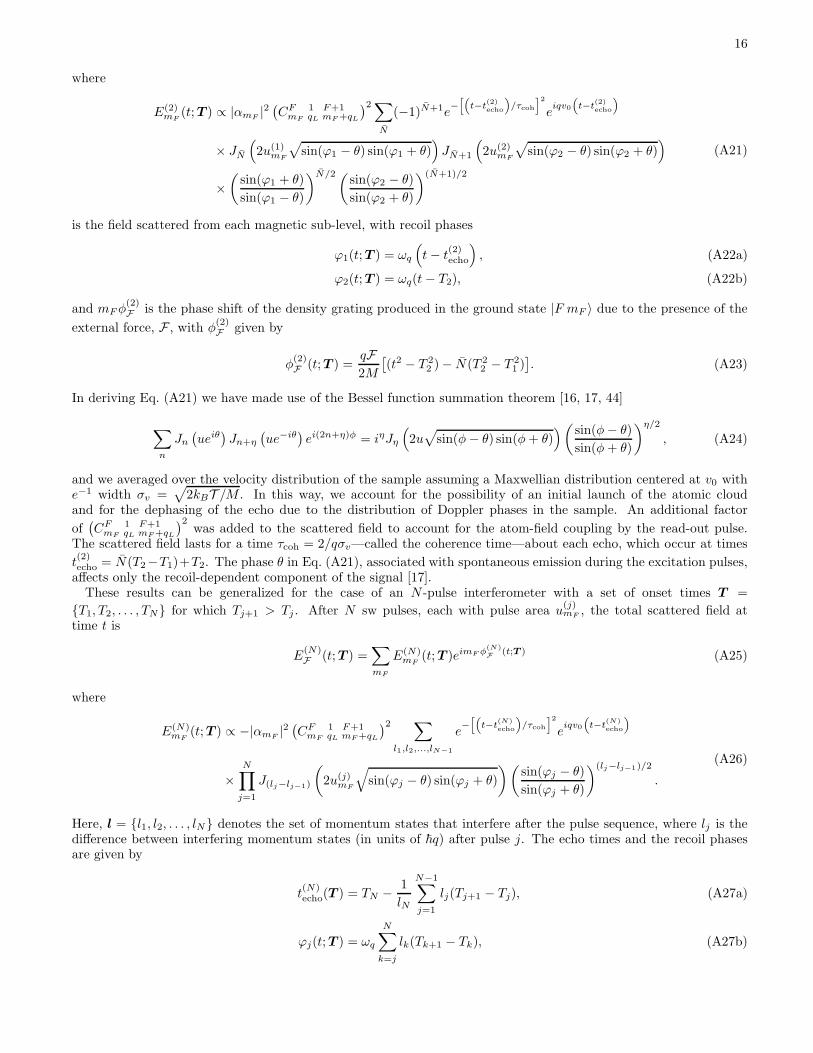
In Eqs. (A26)–(A28) lN = 1, which corresponds to the scattered field from the q-Fourier harmonic of the densityformed after the sw pulses, and it is understood that l0 = 0 and TN+1 = t.We now use the formalism for the N -pulse echo signal [Eq. (A26)] to obtain an expression for the three-pulse

interferometer signal discussed in Sec. II. We begin by setting N = 3 and T = T1, T1 + T21, T1 + T21 + T32. For

an echo to occur at t(3)echo = T1 + T32 + (N + 1)T21 for any T1, T32 and T21, Eq. (A27a) dictates the set of lj to be

l = −N, 0, 1. Then, it can be shown that the scattered field is given by

E(3)mF

(t;T ) ∝ |αmF|2(

CF 1 F+1mF qL mF+qL

)2 ∑

N

(−1)N+1e−[(

t−t(3)echo

)

/τcoh

]2

eiqv0

(

t−t(3)echo

)

× JN

(

2u(1)mF

√

sin(ϕ1 − θ) sin(ϕ1 + θ))

JN

(

2u(2)mF

√

sin(ϕ2 − θ) sin(ϕ2 + θ))

× J1

(

2u(3)mF

√

sin(ϕ3 − θ) sin(ϕ3 + θ))

(

sin(ϕ1 + θ)

sin(ϕ1 − θ)

)N/2 (sin(ϕ2 − θ)

sin(ϕ2 + θ)

)N/2 (sin(ϕ3 − θ)

sin(ϕ3 + θ)

)1/2

,

(A29)

where the recoil phases in this case are

ϕ1 = ωq

(

t− t(3)echo

)

, (A30a)

ϕ2 = ϕ3 = ωq

(

t− t(3)echo + NT21

)

, (A30b)

and the grating phase due to F is

φ(3)F (t;T ) =

qF2M

[

−N(T 22 − T 2

1 ) + (t2 − T 23 )]

=qF2M

N(N + 1)T 221 + 2NT32T21 + 2

[

T1 + T32 + (N + 1)T21

]

∆t+∆t2

. (A31)

[1] M. Kasevich and S. Chu, Phys. Rev. Lett., 67, 181(1991).

[2] A. Peters, K. Y. Chung, and S. Chu, Nature, 400, 849(1999).

[3] A. Peters, K. Y. Chung, and S. Chu, Metrologia, 38, 25(2001).

[4] K. J. Hughes, J. H. T. Burke, and C. A. Sackett, Phys.Rev. Lett., 102, 150403 (2009).

[5] N. Poli, F.-Y. Wang, M. G. Tarallo, A. Alberti,M. Prevedelli, and G. M. Tino, Phys. Rev. Lett., 106,038501 (2011).

[6] M. J. Snadden, J. M. McGuirk, P. Bouyer, K. G. Haritos,and M. A. Kasevich, Phys. Rev. Lett., 81, 971 (1998).

[7] J. M. McGuirk, G. T. Foster, J. B. Fixler, M. J. Snadden,and M. A. Kasevich, Phys. Rev. A, 65, 033608 (2002).

[8] N. Yu, J. M. Kohel, J. R. Kellogg, and L. Maleki, Appl.Phys. B, 84, 647 (2006).

[9] T. L. Gustavson, P. Bouyer, and M. A. Kasevich, Phys.Rev. Lett., 78, 2046 (1997).

[10] S. Wu, E. Su, and M. Prentiss, Phys. Rev. Lett., 99,173201 (2007).

[11] J. H. T. Burke and C. A. Sackett, Phys. Rev. A, 80,

061603 (2009).[12] S. B. Cahn, A. Kumarakrishnan, U. Shim, T. Sleator,

P. R. Berman, and B. Dubetsky, Phys. Rev. Lett., 79,784 (1997).

[13] D. V. Strekalov, A. Turlapov, A. Kumarakrishnan, andT. Sleator, Phys. Rev. A, 66, 023601 (2002).

[14] This condition is true for far off-resonant excitation fieldsonly. For fields closer to resonance, both the AC Starkeffect and the Zeeman effect can induce a relative shiftbetween the ground and excited states, thus affecting theresponse of the interferometer in a systematic way.

[15] E. J. Su, S. Wu, and M. G. Prentiss, Phys. Rev. A, 81,043631 (2010).

[16] S. Beattie, B. Barrett, M. Weel, I. Chan, C. Mok, S. B.Cahn, and A. Kumarakrishnan, Phys. Rev. A, 77,013610 (2008).

[17] B. Barrett, I. Yavin, S. Beattie, and A. Kumarakrishnan,Phys. Rev. A, 82, 023625 (2010).

[18] T. W. Mossberg, R. Kachru, S. R. Hartmann, and A. M.Flusberg, Phys. Rev. A, 20, 1976 (1979).

[19] C. J. Borde, C. Salomon, S. Avrillier, A. Van Lerberghe,C. Breant, D. Bassi, and G. Scoles, Phys. Rev. A, 30,

18

1836 (1984).[20] L. Allen and J. H. Eberly, Optical Resonance and Two-

Level Atoms (Dover, New York, 1987).[21] B. Dubetsky, P. R. Berman, and T. Sleator, Phys. Rev.

A, 46, R2213 (1992).[22] B. Barrett, I. Chan, C. Mok, A. Carew, I. Yavin, A. Ku-

marakrishnan, S. B. Cahn, and T. Sleator, Time Do-

main Interferometry With Laser Cooled Atoms, edited byE. Arimondo, P. R. Berman, and C. C. Lin, Advances inAtomic, Molecular and Optical Physics, Vol. 60 (Elsevier,2011) Chap. 3.

[23] M. Weel and A. Kumarakrishnan, Phys. Rev. A, 67,061602(R) (2003).

[24] S. Beattie, B. Barrett, I. Chan, C. Mok, I. Yavin, andA. Kumarakrishnan, Phys. Rev. A, 79, 021605(R) (2009).

[25] S. Beattie, B. Barrett, I. Chan, C. Mok, I. Yavin, andA. Kumarakrishnan, Phys. Rev. A, 80, 013618 (2009).

[26] B. Barrett, S. Beattie, A. Carew, I. Chan, C. Mok,I. Yavin, and A. Kumarakrishnan, in ICONO 2010: In-

ternational Conference on Coherent and Nonlinear Op-

tics, Proc. of SPIE, Vol. 7993, edited by C. Fabre, V. Zad-kov, and K. Drabovich (2011) pp. 79930Y–1.

[27] M. Weel, I. Chan, S. Beattie, A. Kumarakrishnan,D. Gosset, and I. Yavin, Phys. Rev. A, 73, 063624(2006).

[28] M. F. Andersen and T. Sleator, Phys. Rev. Lett., 103,070402 (2009).

[29] A. Wicht, J. M. Hensley, E. Sarajlic, and S. Chu, Phys.Scr., T102, 82 (2002).

[30] I. Chan, B. Barrett, and A. Kumarakrishnan, Phys. Rev.A, 84, 032509 (2011).

[31] J. P. Davis and F. A. Narducci, J. Mod. Opt., 55, 3173

(2008).[32] T. M. Roach, J. Phys. B, 37, 3551 (2004).[33] D. S. Weiss, E. Riss, Y. Shevy, P. J. Ungar, and S. Chu,

J. Opt. Soc. Am. B, 6, 2072 (1989).[34] A. Vorozcovs, M. Weel, S. Beattie, S. Cauchi, and A. Ku-

marakrishnan, J. Opt. Soc. Am. B, 22, 943 (2005).[35] S. Slama, C. von Cube, M. Kohler, C. Zimmermann, and

P. W. Courteille, Phys. Rev. A, 73, 023424 (2006).[36] A. Schilke, C. Zimmermann, P. W. Courteille, and

W. Guerin, Phys. Rev. Lett., 106, 223903 (2011).[37] J. M. Anthony and K. J. Sebastian, Phys. Rev. A, 49,

192 (1994).[38] Measurements of the B-gradient from the scattered field

intensity are not sensitive to the sign of β. However, thesign can be determined using a heterodyne technique tomeasure the scattered electric field amplitude.

[39] T. M. Niebauer, G. S. Sasagawa, J. E. Faller, R. Hilt,and F. Klopping, Metrologia, 32, 159 (1995).

[40] J. Le Gouet, T. E. Mehlstaubler, J. Kim, S. Merlet,A. Clairon, A. Landragin, and F. P. D. Santos, Appl.Phys. B, 92, 133 (2008).

[41] B. Young, D. S. Bonomi, T. Patterson, F. Roller, T. Tran,A. Vitouchkine, T. Gustavson, and M. Kasevich, in Pro-

ceedings of the International Conference on Laser Science

(Optical Society of America, 2007) p. LTuH1.[42] M. Suzuki, Commun. Math. Phys., 57, 193 (1977).[43] This choice is not arbitrary. Since the p-space wave

function is an eigenstate of the operator p2/2M , but

not −Mz, we save ourselves some effort by choosing

B = p2/2M since eB operates on the wave function be-

fore eA.[44] I. S. Gradshteyn and I. M. Ryzhik, Tables of Integrals,

Series, and Products, 7th ed. (Elsevier, 2007) p. 940.