Embed Size (px)
Citation preview

Review
Belief and Probability• The connection between toothaches and cavities is not a logical
consequence in either direction.
• However, we can provide a degree of belief on the sentences.– We usually get this belief from statistical data.
• Assigning probability 0 to a sentence correspond to an unequivocal belief that the sentence is false.
• Assigning probability 1 to a sentence correspond to an unequivocal belief that the sentence is true.
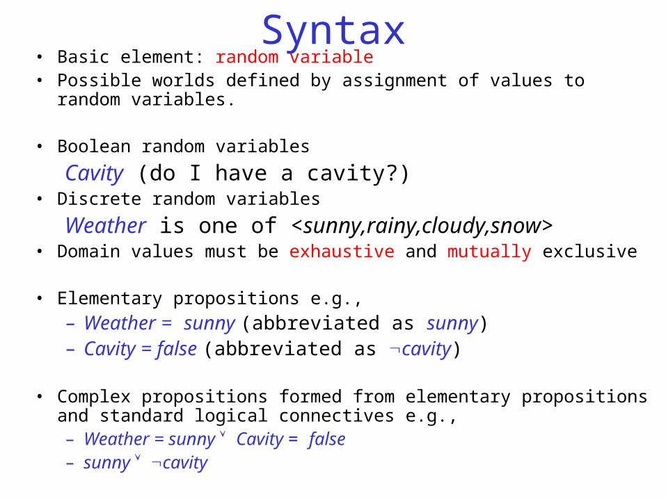
Syntax• Basic element: random variable• Possible worlds defined by assignment of values to random variables.
• Boolean random variables
Cavity (do I have a cavity?)• Discrete random variables
Weather is one of <sunny,rainy,cloudy,snow>• Domain values must be exhaustive and mutually exclusive
• Elementary propositions e.g.,
– Weather = sunny (abbreviated as sunny) – Cavity = false (abbreviated as cavity)
• Complex propositions formed from elementary propositions and standard logical connectives e.g., – Weather = sunny Cavity = false– sunny cavity
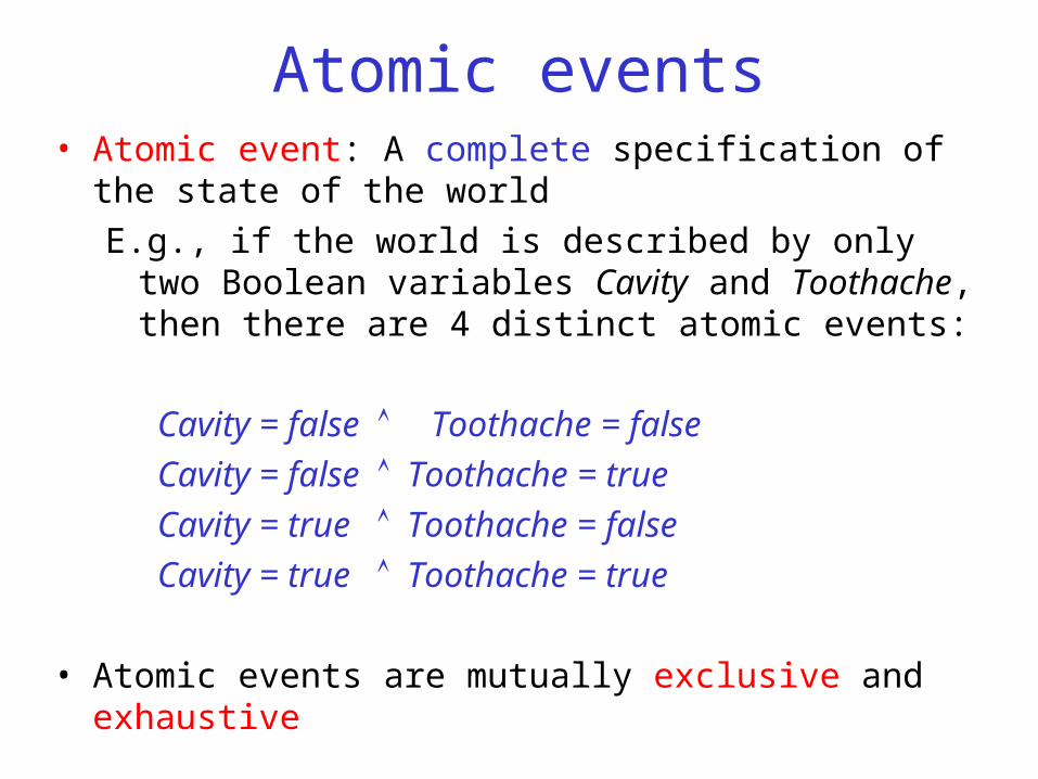
Atomic events• Atomic event: A complete specification of the state of the world
E.g., if the world is described by only two Boolean variables Cavity and Toothache, then there are 4 distinct atomic events:
Cavity = false Toothache = false
Cavity = false Toothache = true
Cavity = true Toothache = false
Cavity = true Toothache = true
• Atomic events are mutually exclusive and exhaustive
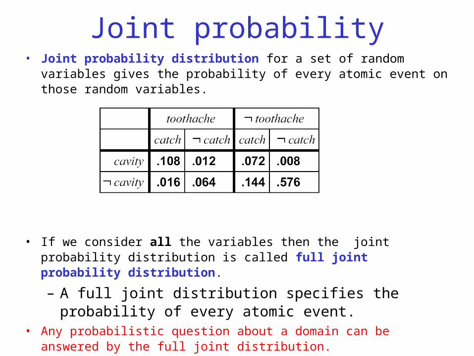
Joint probability• Joint probability distribution for a set of random variables gives the
probability of every atomic event on those random variables.
• If we consider all the variables then the joint probability distribution is called full joint probability distribution.
– A full joint distribution specifies the probability of every atomic event.
• Any probabilistic question about a domain can be answered by the full joint distribution.
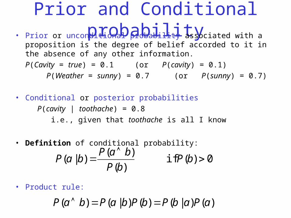
Prior and Conditional probability• Prior or unconditional probability associated with a proposition is the degree
of belief accorded to it in the absence of any other information.
P(Cavity = true) = 0.1 (or P(cavity) = 0.1)
P(Weather = sunny) = 0.7 (or P(sunny) = 0.7)
• Conditional or posterior probabilities
P(cavity | toothache) = 0.8
i.e., given that toothache is all I know
• Definition of conditional probability:
• Product rule:
0)( if )(
)()|(
bP
bP
baPbaP
)()|()()|()( aPabPbPbaPbaP
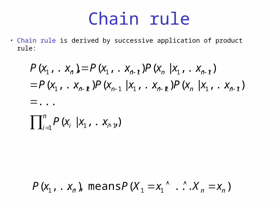
Chain rule• Chain rule is derived by successive application of product rule:
n
i ii
nnnnn
nnnn
xxxP
xxxPxxxPxxP
xxxPxxPxxP
1 11
1121121
11111
),...,|(
...
),...,|(),...,|(),...,(
),...,|(),...,(),...,(
)...( means ),...,( 111 nnn xXxXPxxP
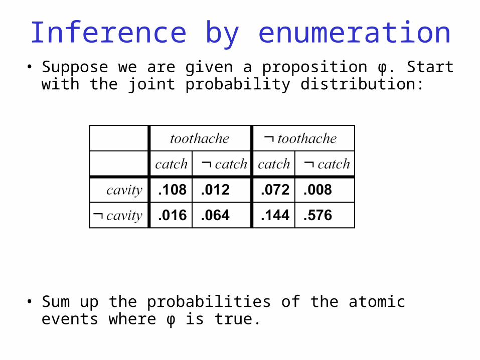
Inference by enumeration• Suppose we are given a proposition φ. Start with the joint
probability distribution:
• Sum up the probabilities of the atomic events where φ is true.
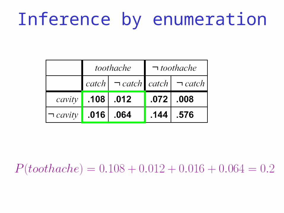
Inference by enumeration
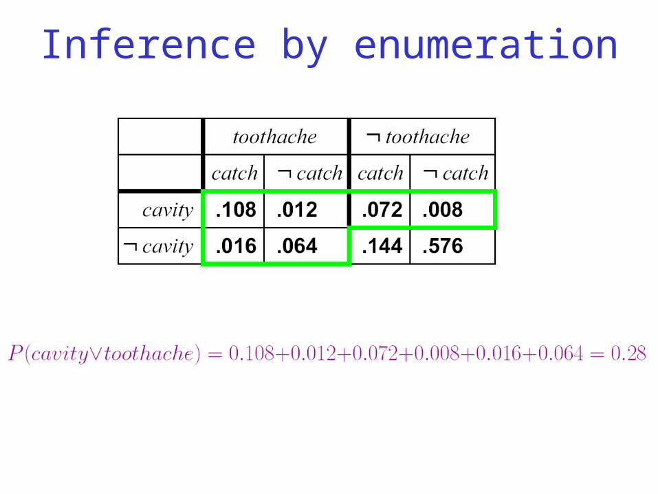
Inference by enumeration
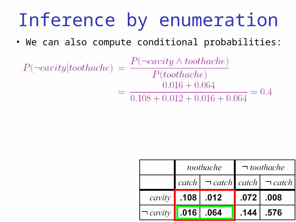
Inference by enumeration• We can also compute conditional probabilities:
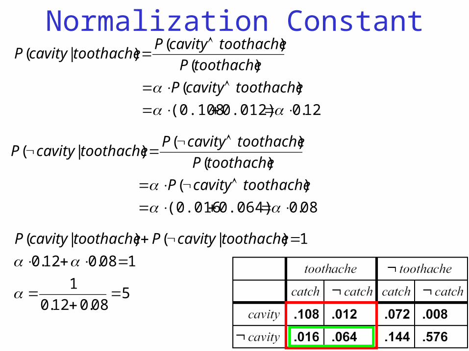
Normalization Constant
12.0 0.012)(0.108
)(
)(
)()|(
toothachecavityP
toothacheP
toothachecavityPtoothachecavityP
08.0 0.064)(0.016
)(
)(
)()|(
toothachecavityP
toothacheP
toothachecavityPtoothachecavityP
508.012.0
1
108.012.0
1)|()|(
toothachecavityPtoothachecavityP
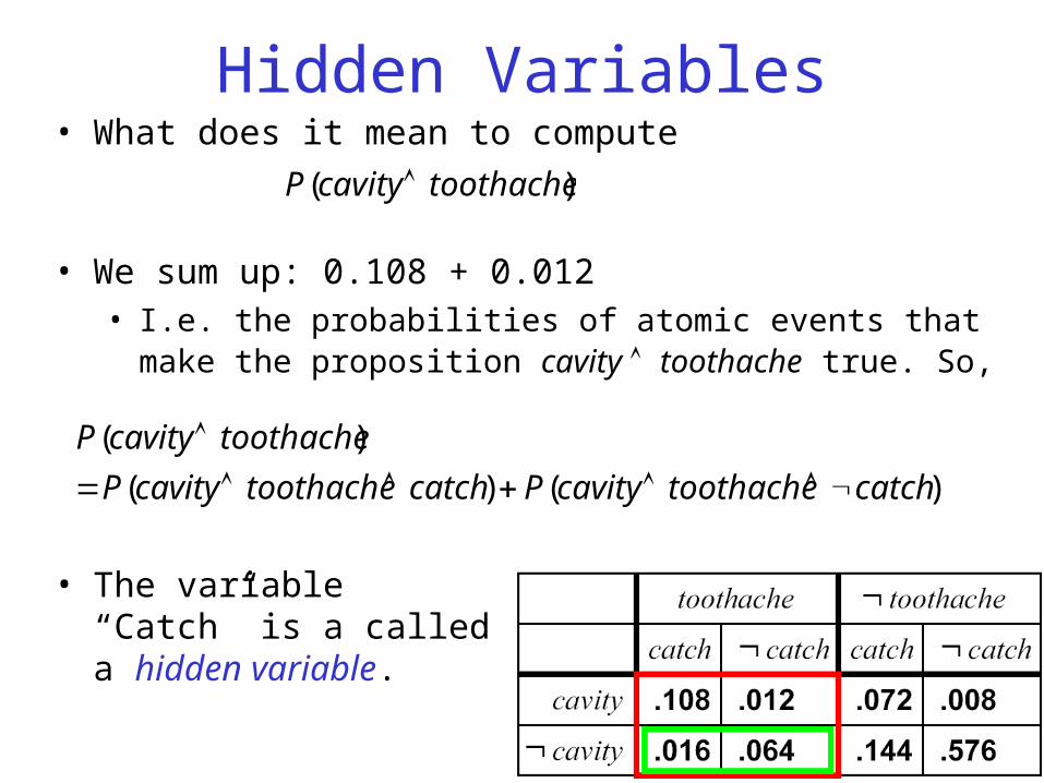
Hidden Variables• What does it mean to compute
)( toothachecavityP
• We sum up: 0.108 + 0.012• I.e. the probabilities of atomic events that make the proposition
cavity toothache true. So,
)()(
)(
catchtoothachecavityPcatchtoothachecavityP
toothachecavityP
• The variable “Catch” is a called a hidden variable.
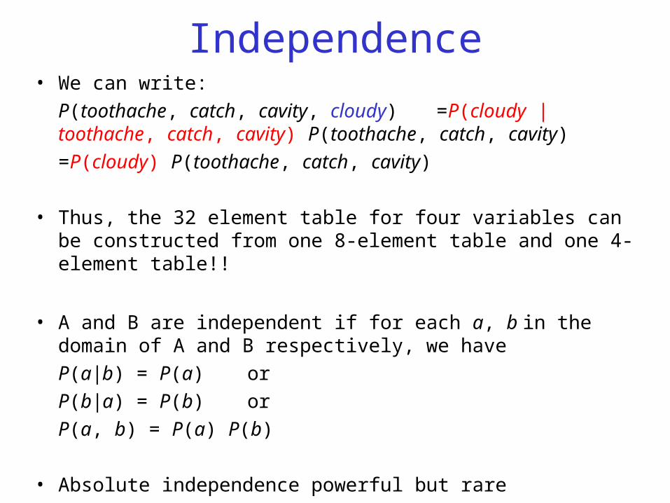
Independence• We can write:
P(toothache, catch, cavity, cloudy) =P(cloudy | toothache, catch, cavity) P(toothache, catch, cavity)
=P(cloudy) P(toothache, catch, cavity)
• Thus, the 32 element table for four variables can be constructed from one 8-element table and one 4-element table!!
• A and B are independent if for each a, b in the domain of A and B respectively, we have
P(a|b) = P(a) or
P(b|a) = P(b) or
P(a, b) = P(a) P(b)
• Absolute independence powerful but rare
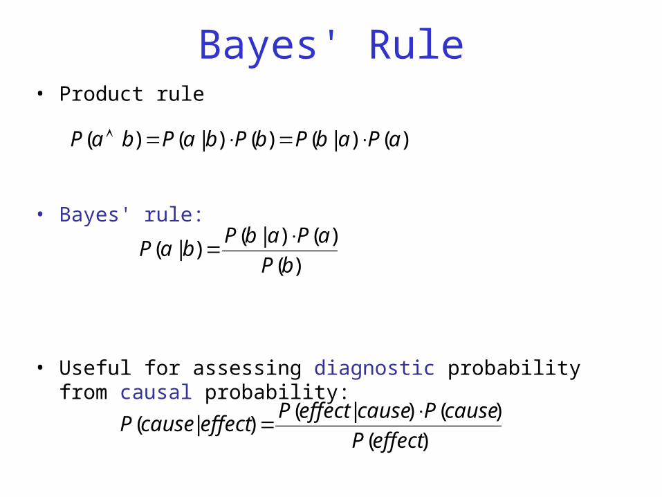
Bayes' Rule• Product rule
• Bayes' rule:
• Useful for assessing diagnostic probability from causal probability:
)()|()()|()( aPabPbPbaPbaP
)(
)()|()|(
bP
aPabPbaP
)(
)()|()|(
effectP
causePcauseeffectPeffectcauseP
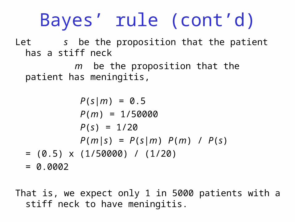
Bayes’ rule (cont’d)Let s be the proposition that the patient has a stiff neck
m be the proposition that the patient has meningitis,
P(s|m) = 0.5
P(m) = 1/50000
P(s) = 1/20
P(m|s) = P(s|m) P(m) / P(s)
= (0.5) x (1/50000) / (1/20)
= 0.0002
That is, we expect only 1 in 5000 patients with a stiff neck to have meningitis.
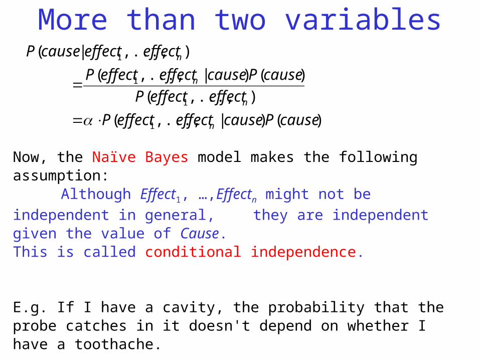
More than two variables
)()|,...,(
),...,(
)()|,...,(
),...,|(
1
1
1
1
causePcauseeffecteffectP
effecteffectP
causePcauseeffecteffectP
effecteffectcauseP
n
n
n
n
Now, the Naïve Bayes model makes the following assumption:Although Effect1, …,Effectn might not be independent in general,
they are independent given the value of Cause. This is called conditional independence.
E.g. If I have a cavity, the probability that the probe catches in it doesn't depend on whether I have a toothache.
We write this as: P(toothache, catch | cavity) = P(toothache | cavity) . P(catch | cavity) . P(cavity)
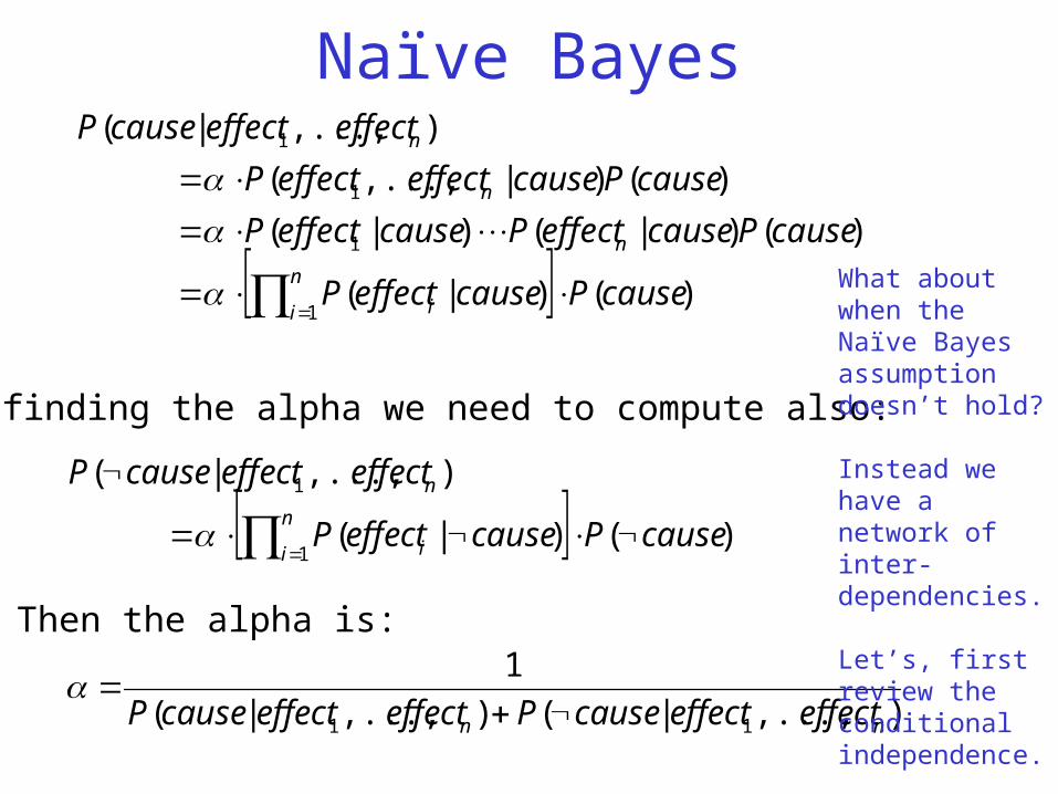
Naïve Bayes
)()|(
)()|()|(
)()|,...,(
),...,|(
1
1
1
1
causePcauseeffectP
causePcauseeffectPcauseeffectP
causePcauseeffecteffectP
effecteffectcauseP
n
i i
n
n
n
For finding the alpha we need to compute also:
)()|(
),...,|(
1
1
causePcauseeffectP
effecteffectcausePn
i i
n
Then the alpha is:
),...,|(),...,|(
1
11 nn effecteffectcausePeffecteffectcauseP
What about when the Naïve Bayes assumption doesn’t hold?
Instead we have a network of inter-dependencies.
Let’s, first review the conditional independence.
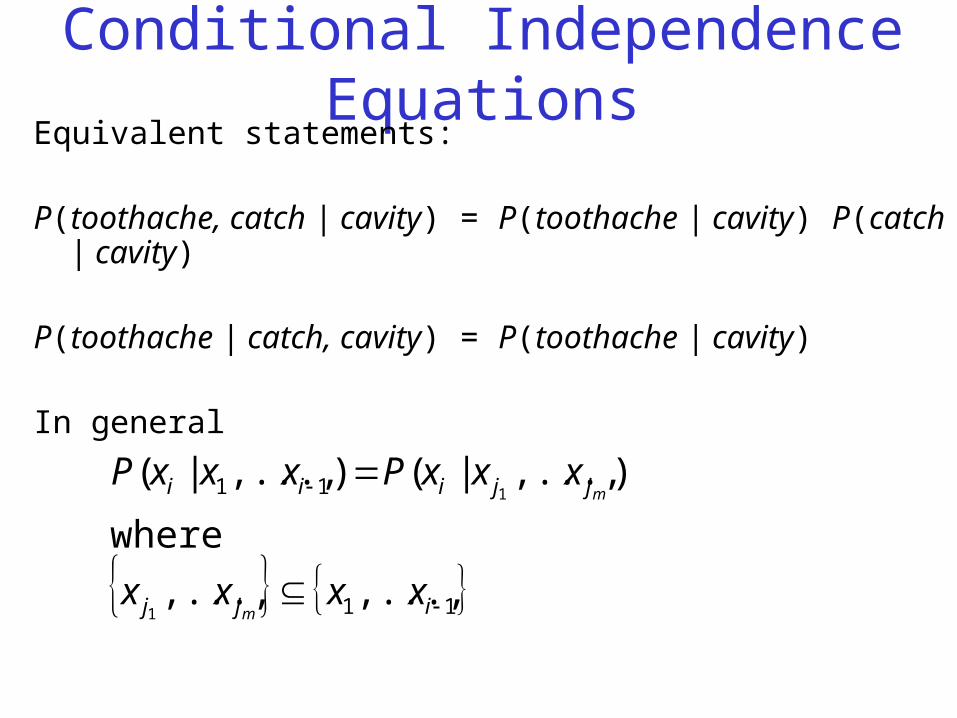
Conditional Independence EquationsEquivalent statements:
P(toothache, catch | cavity) = P(toothache | cavity) P(catch | cavity)
P(toothache | catch, cavity) = P(toothache | cavity)
In general
11
11
,...,,...,
where
),...,|(),...,|(
1
1
ijj
jjiii
xxxx
xxxPxxxP
m
m
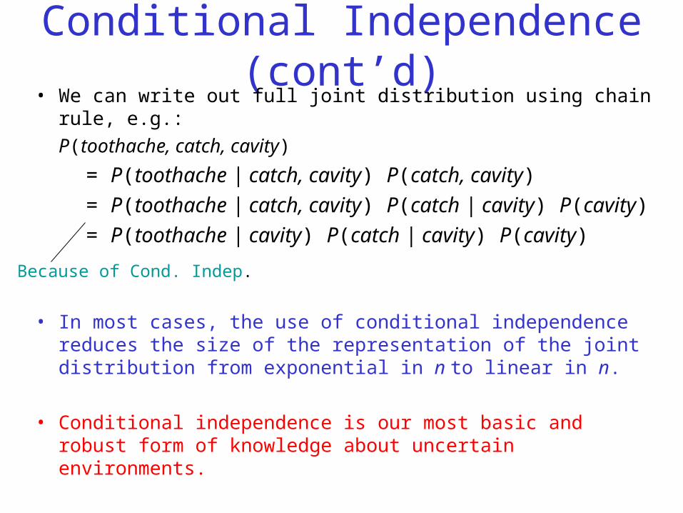
Conditional Independence (cont’d)• We can write out full joint distribution using chain rule, e.g.:
P(toothache, catch, cavity)
= P(toothache | catch, cavity) P(catch, cavity)
= P(toothache | catch, cavity) P(catch | cavity) P(cavity)
= P(toothache | cavity) P(catch | cavity) P(cavity)
• In most cases, the use of conditional independence reduces the size of the representation of the joint distribution from exponential in n to linear in n.
• Conditional independence is our most basic and robust form of knowledge about uncertain environments.
Because of Cond. Indep.
Bayesian Networks: Motivation
• The full joint probability can be used to answer any question about the domain, – but intractable as the number of variables grow.
• Furthermore specifying probabilities of atomic events is rather unnatural and can be very difficult.
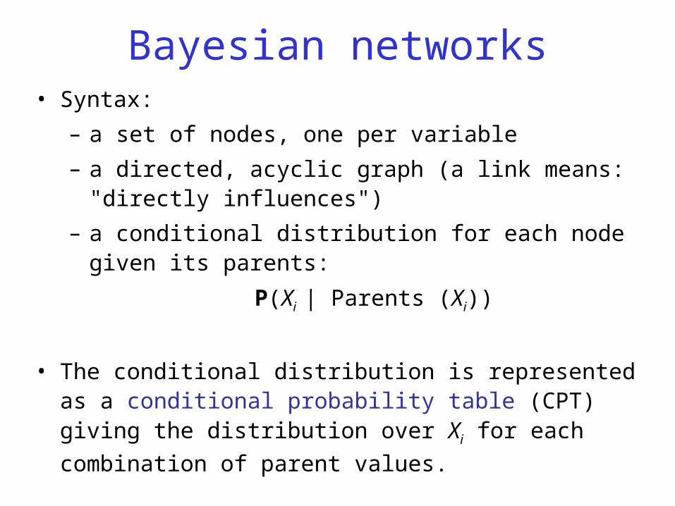
Bayesian networks• Syntax:
– a set of nodes, one per variable
– a directed, acyclic graph (a link means: "directly influences")
– a conditional distribution for each node given its parents:
P(Xi | Parents (Xi))
• The conditional distribution is represented as a conditional probability table (CPT) giving the distribution over Xi for each
combination of parent values.
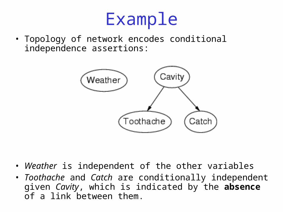
Example• Topology of network encodes conditional independence
assertions:
• Weather is independent of the other variables• Toothache and Catch are conditionally independent given
Cavity, which is indicated by the absence of a link between them.
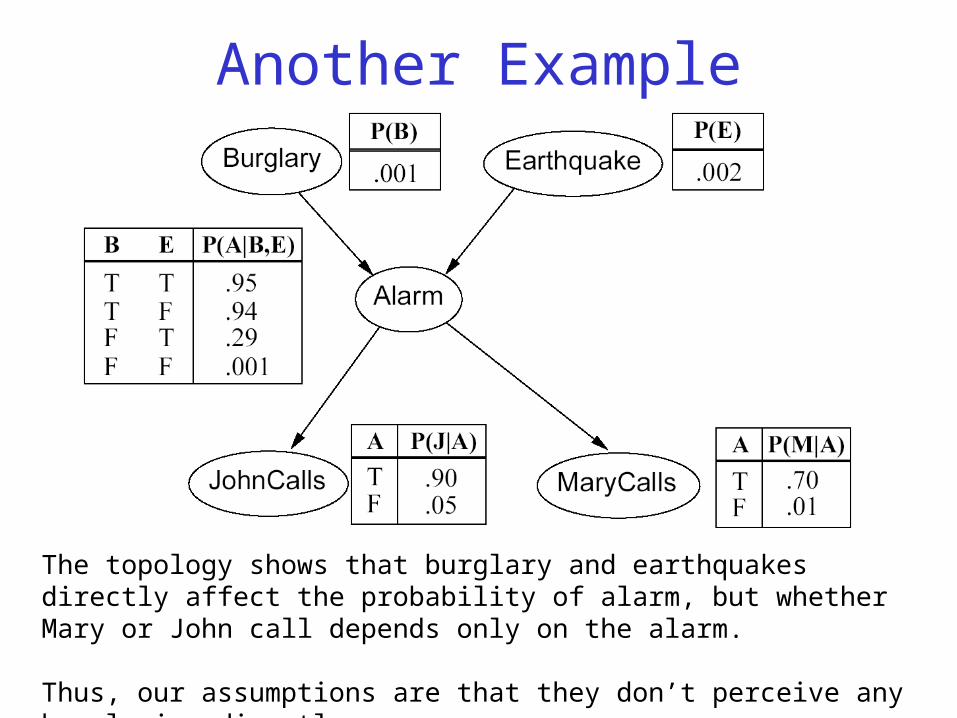
Another Example
The topology shows that burglary and earthquakes directly affect the probability of alarm, but whether Mary or John call depends only on the alarm.
Thus, our assumptions are that they don’t perceive any burglaries directly, and they don’t confer before calling.
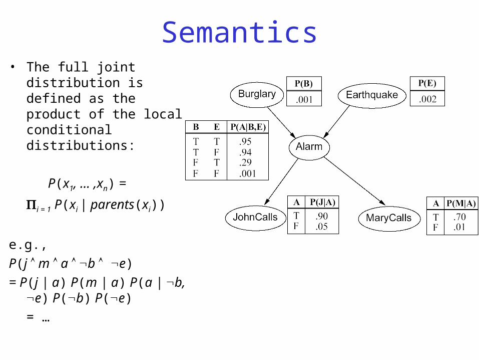
Semantics• The full joint distribution is
defined as the product of the local conditional distributions:
P(x1, … ,xn) =
i = 1 P(xi | parents(xi))
e.g.,
P(j m a b e)
= P(j | a) P(m | a) P(a | b, e) P(b) P(e)
= …
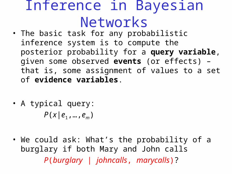
Inference in Bayesian Networks• The basic task for any probabilistic inference system is to
compute the posterior probability for a query variable, given some observed events (or effects) – that is, some assignment of values to a set of evidence variables.
• A typical query:
P(x|e1,…,em)
• We could ask: What’s the probability of a burglary if both Mary and John calls
P(burglary | johncalls, marycalls)?
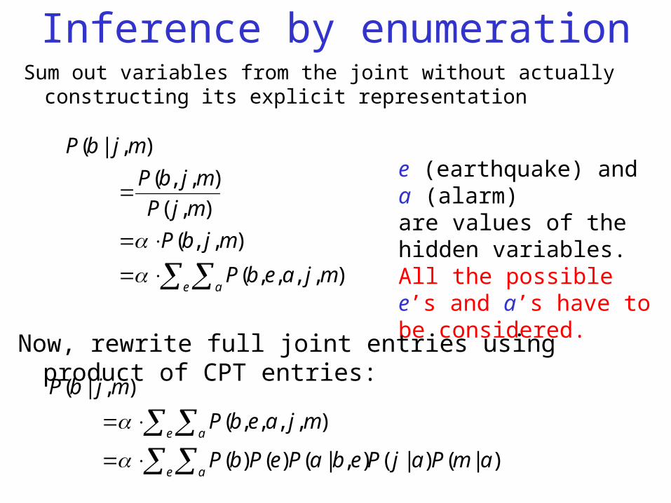
Inference by enumerationSum out variables from the joint without actually
constructing its explicit representation
e amjaebP
mjbP
mjP
mjbP
mjbP
),,,,(
),,(
),(
),,(
),|(
e (earthquake) and a (alarm)are values of the hidden variables.All the possible e’s and a’s have to be considered.
Now, rewrite full joint entries using product of CPT entries:
)|()|(),|()()(
),,,,(
),|(
amPajPebaPePbP
mjaebP
mjbP
e a
e a
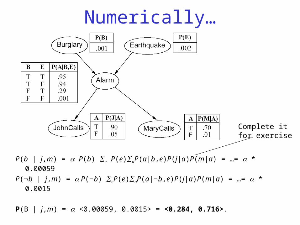
Numerically…
P(b | j,m) = P(b) e P(e)aP(a|b,e)P(j|a)P(m|a) = …= * 0.00059
P(b | j,m) = P(b) eP(e)aP(a|b,e)P(j|a)P(m|a) = …= * 0.0015
P(B | j,m) = <0.00059, 0.0015> = <0.284, 0.716>.
Complete it for exercise
Machine Learning
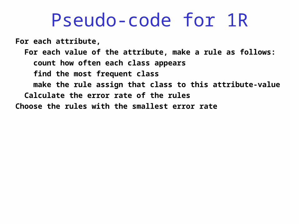
Pseudo-code for 1RFor each attribute,
For each value of the attribute, make a rule as follows:
count how often each class appears
find the most frequent class
make the rule assign that class to this attribute-value
Calculate the error rate of the rules
Choose the rules with the smallest error rate
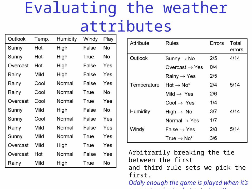
Evaluating the weather attributes
Arbitrarily breaking the tie between the firstand third rule sets we pick the first.Oddly enough the game is played when it’s overcast and rainy but not when it’s sunny. Perhaps it’s an indoor pursuit.
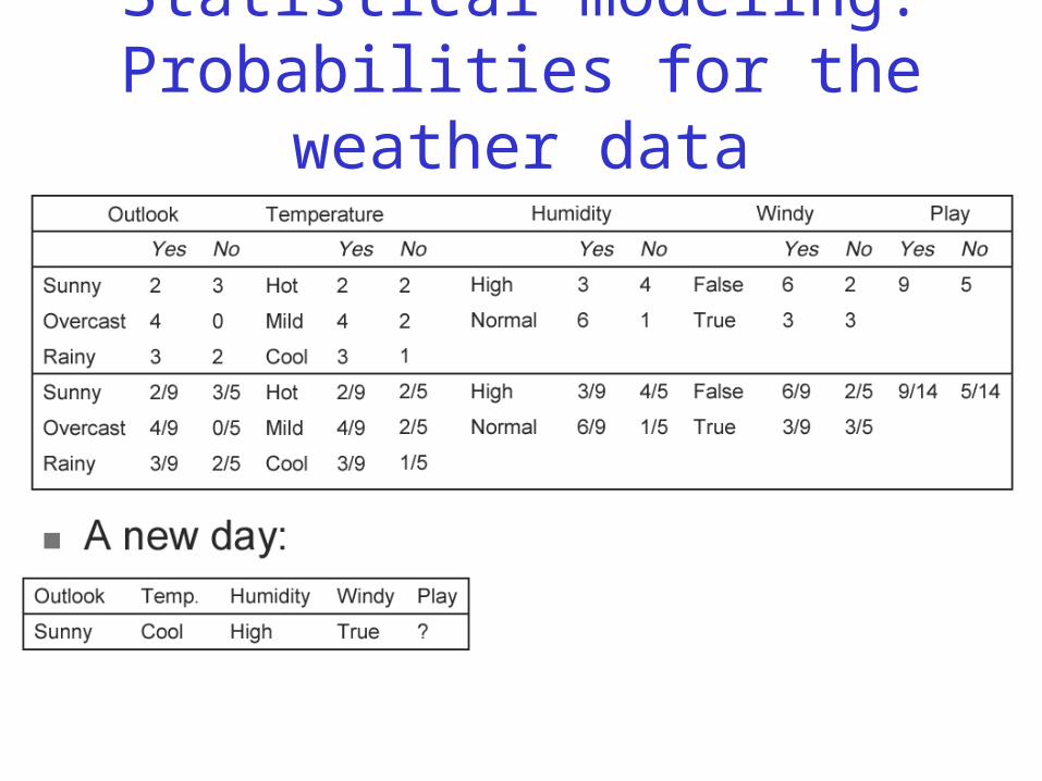
Statistical modeling: Probabilities for the weather data
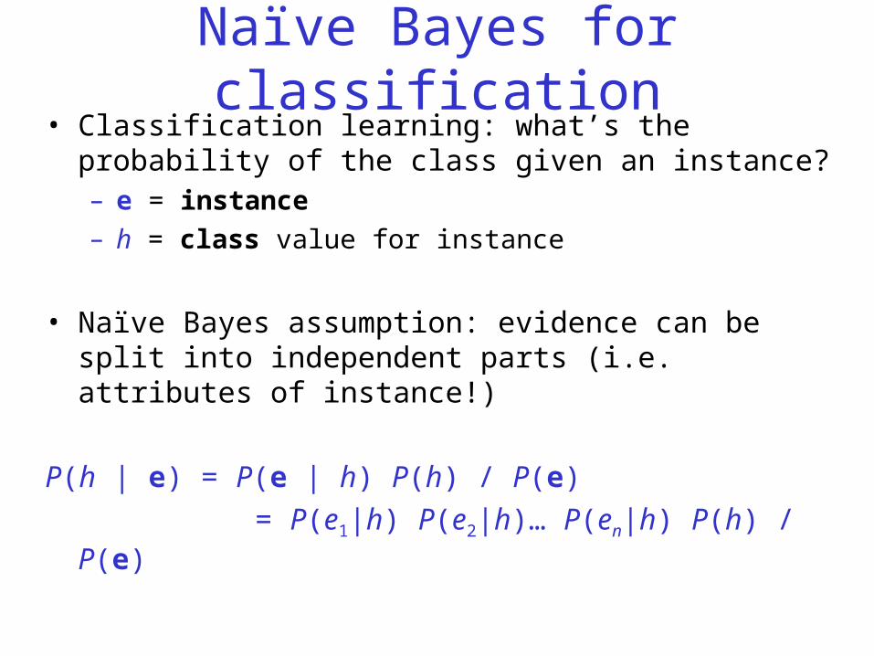
Naïve Bayes for classification• Classification learning: what’s the probability of the class
given an instance?– e = instance
– h = class value for instance
• Naïve Bayes assumption: evidence can be split into independent parts (i.e. attributes of instance!)
P(h | e) = P(e | h) P(h) / P(e)
= P(e1|h) P(e2|h)… P(en|h) P(h) / P(e)
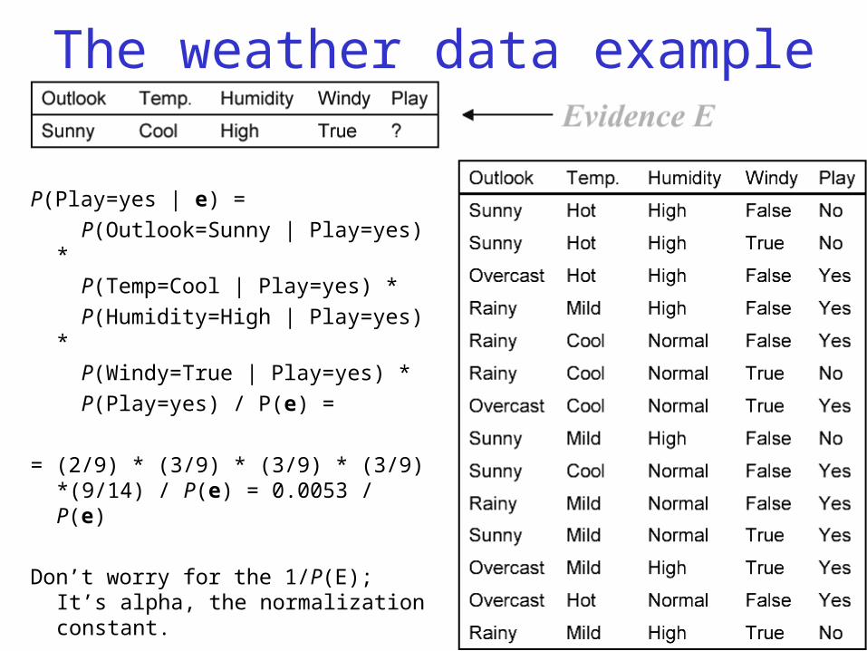
The weather data example
P(Play=yes | e) =
P(Outlook=Sunny | Play=yes) *
P(Temp=Cool | Play=yes) *
P(Humidity=High | Play=yes) *
P(Windy=True | Play=yes) *
P(Play=yes) / P(e) =
= (2/9) * (3/9) * (3/9) * (3/9) *(9/14) / P(e) = 0.0053 / P(e)
Don’t worry for the 1/P(E); It’s alpha, the normalization constant.
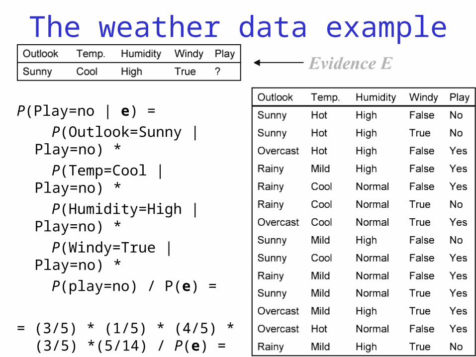
The weather data example
P(Play=no | e) =
P(Outlook=Sunny | Play=no) *
P(Temp=Cool | Play=no) *
P(Humidity=High | Play=no) *
P(Windy=True | Play=no) *
P(play=no) / P(e) =
= (3/5) * (1/5) * (4/5) * (3/5) *(5/14) / P(e) = 0.0206 / P(e)
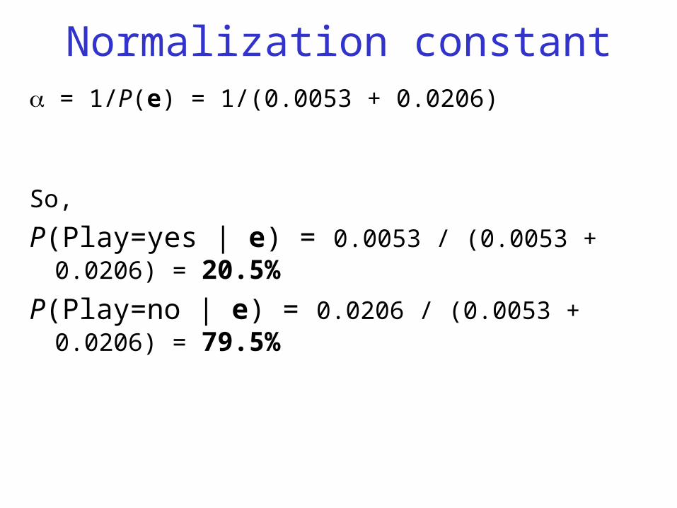
Normalization constant = 1/P(e) = 1/(0.0053 + 0.0206)
So,
P(Play=yes | e) = 0.0053 / (0.0053 + 0.0206) = 20.5%
P(Play=no | e) = 0.0206 / (0.0053 + 0.0206) = 79.5%
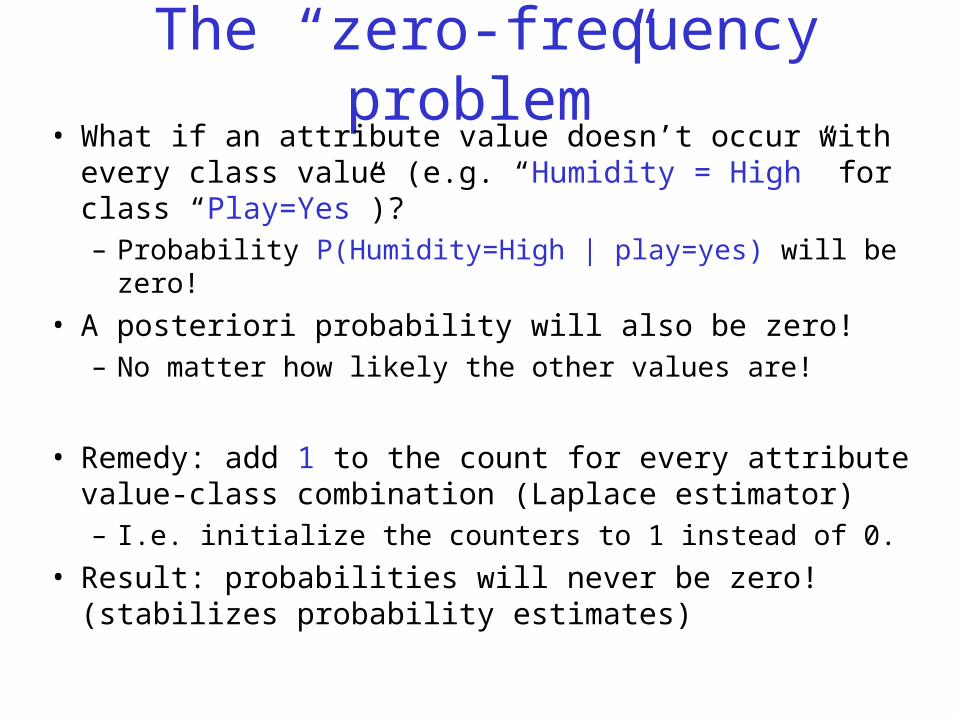
The “zero-frequency problem”• What if an attribute value doesn’t occur with every class
value (e.g. “Humidity = High” for class “Play=Yes”)?– Probability P(Humidity=High | play=yes) will be zero!
• A posteriori probability will also be zero! – No matter how likely the other values are!
• Remedy: add 1 to the count for every attribute value-class combination (Laplace estimator)– I.e. initialize the counters to 1 instead of 0.
• Result: probabilities will never be zero! (stabilizes probability estimates)
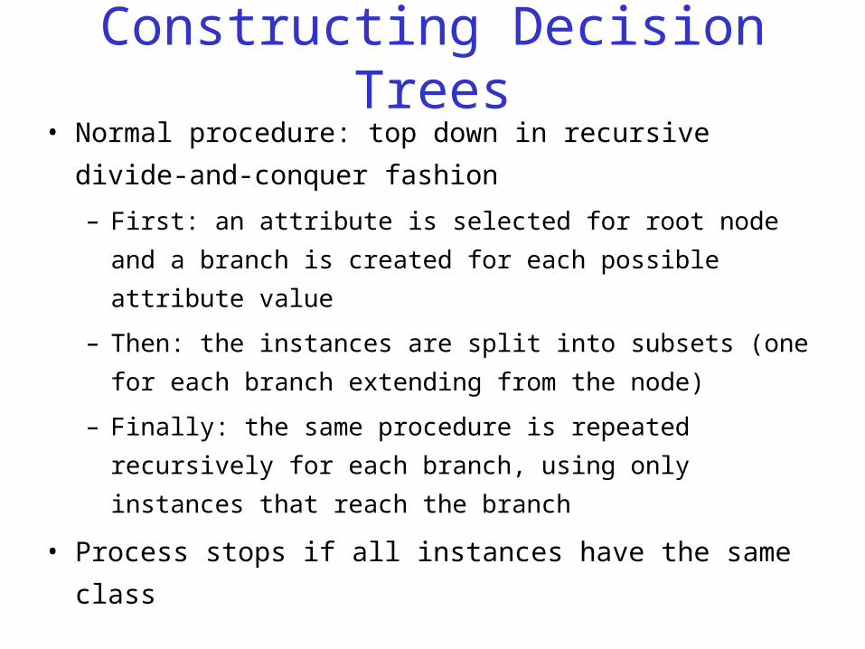
Constructing Decision Trees• Normal procedure: top down in recursive divide-and-
conquer fashion
– First: an attribute is selected for root node and a branch is
created for each possible attribute value
– Then: the instances are split into subsets (one for each
branch extending from the node)
– Finally: the same procedure is repeated recursively for each
branch, using only instances that reach the branch
• Process stops if all instances have the same class
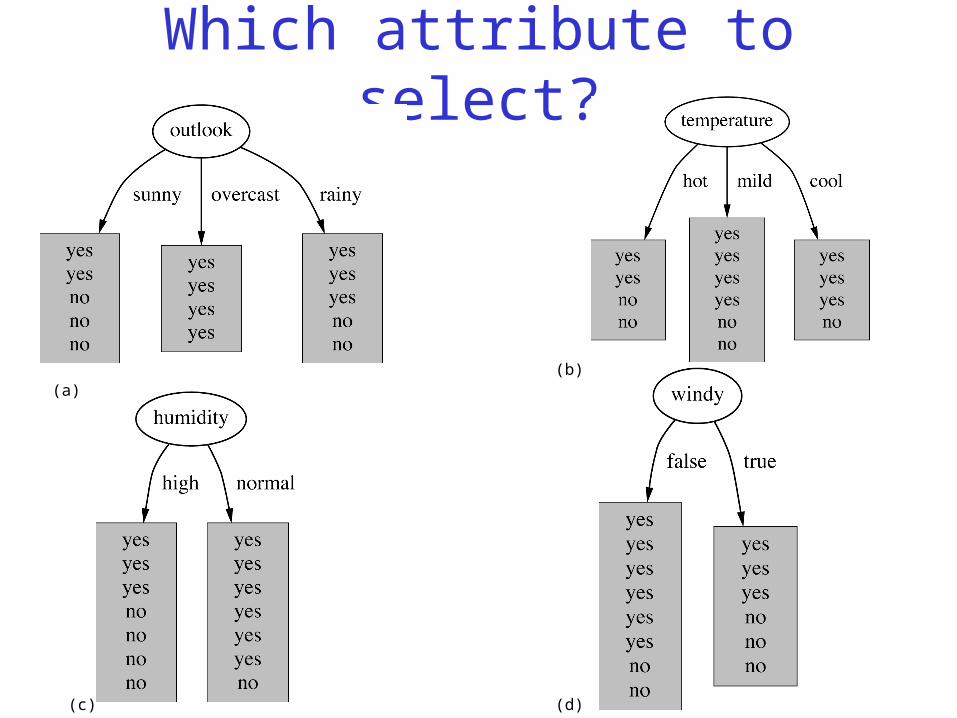
Which attribute to select?
(a)(b)
(c) (d)
A criterion for attribute selection• Which is the best attribute?
• The one which will result in the smallest tree– Heuristic: choose the attribute that produces the “purest”
nodes
• Popular impurity criterion: entropy of nodes– Lower the entropy purer the node.
• Strategy: choose attribute that results in lowest entropy of the children nodes.
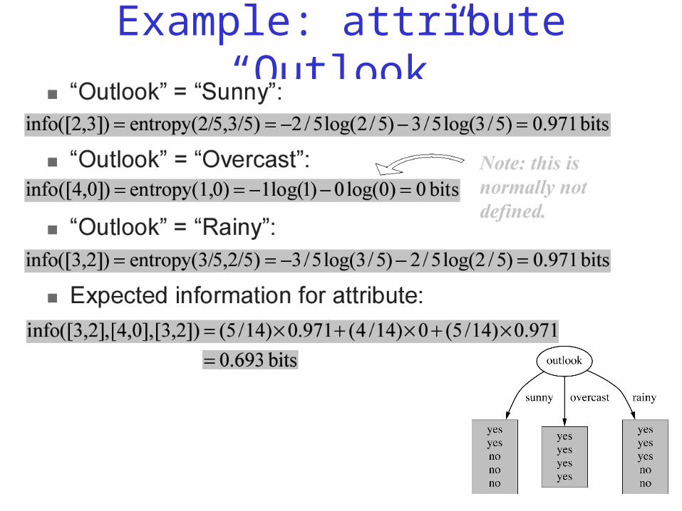
Example: attribute “Outlook”
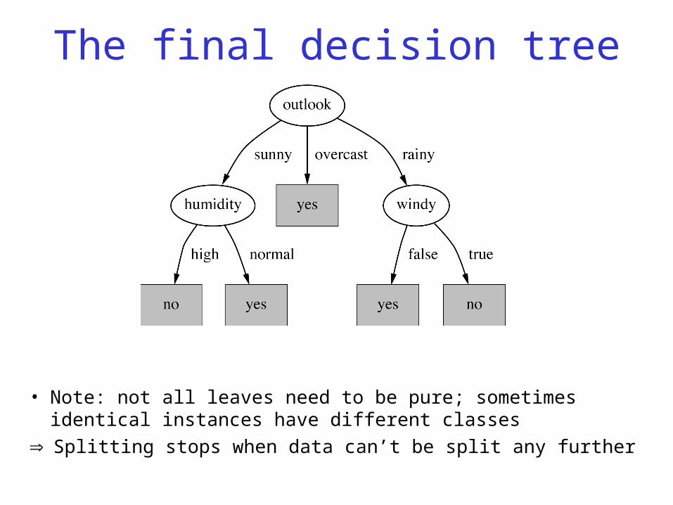
The final decision tree
• Note: not all leaves need to be pure; sometimes identical instances have different classes
Splitting stops when data can’t be split any further
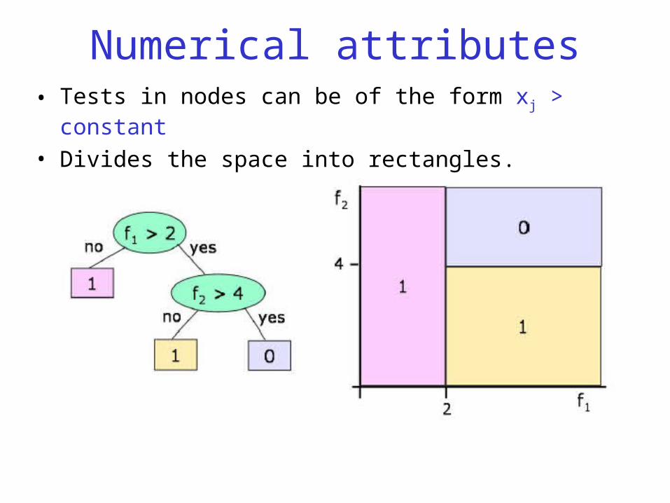
Numerical attributes• Tests in nodes can be of the form xj > constant
• Divides the space into rectangles.
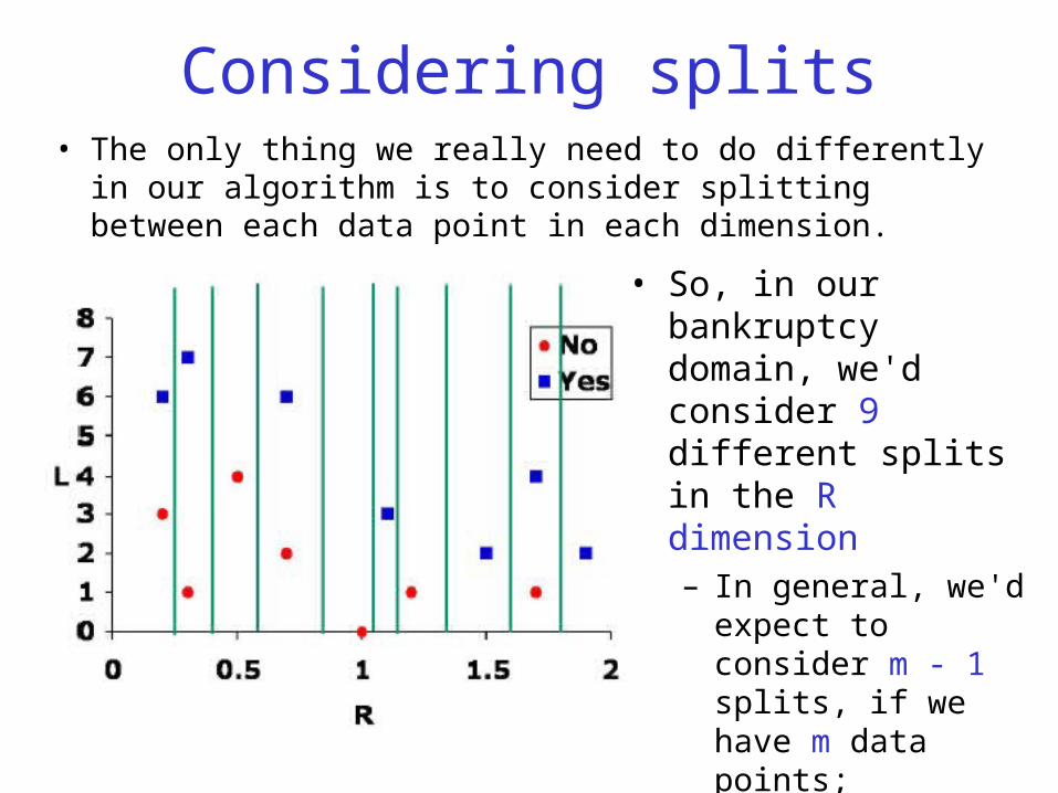
Considering splits• The only thing we really need to do differently in our algorithm
is to consider splitting between each data point in each dimension.
• So, in our bankruptcy domain, we'd consider 9 different splits in the R dimension – In general, we'd expect to
consider m - 1 splits, if we have m data points;
– But in our data set we have some examples with equal R values.
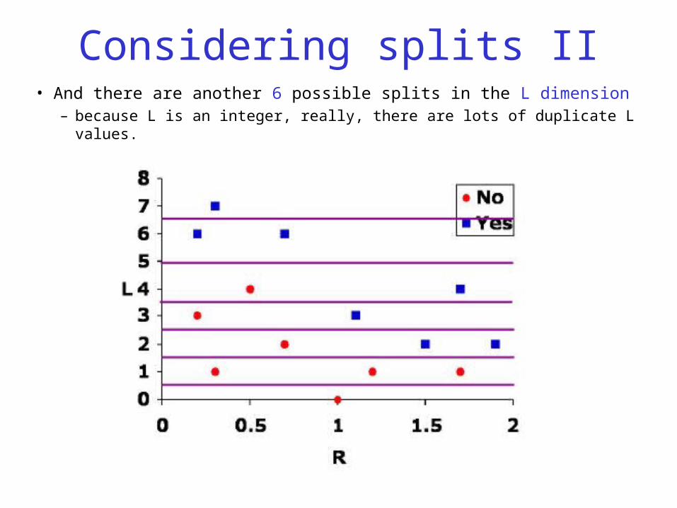
Considering splits II• And there are another 6 possible splits in the L dimension
– because L is an integer, really, there are lots of duplicate L values.
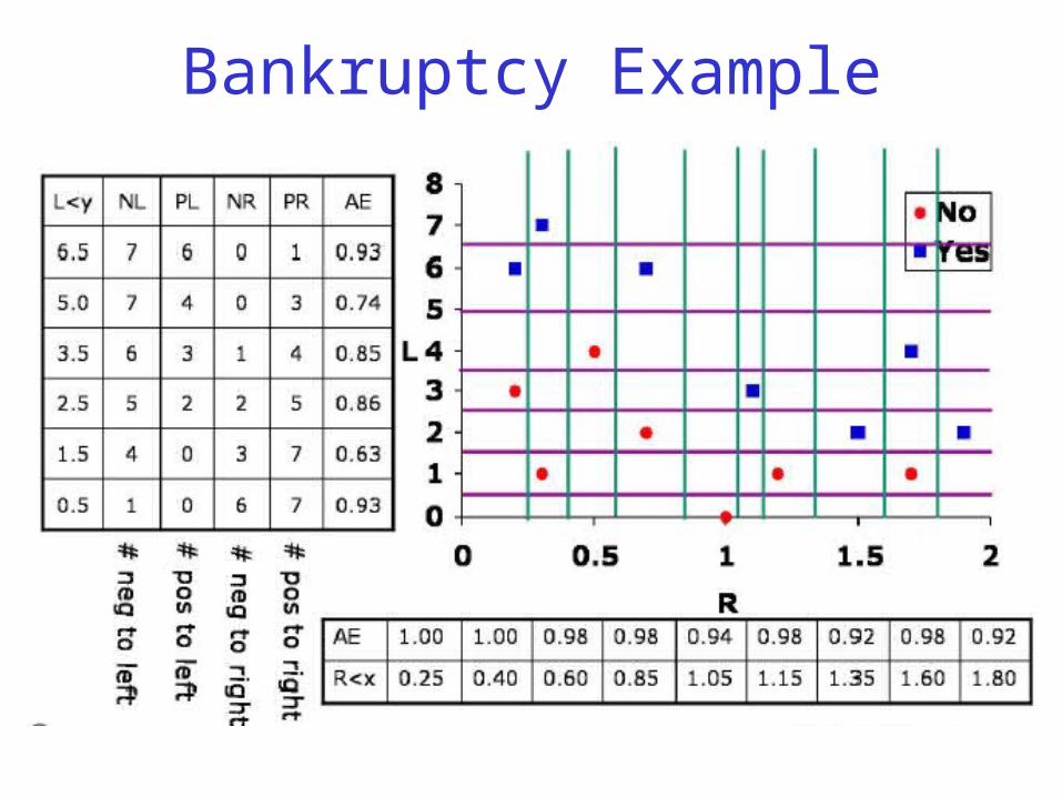
Bankruptcy Example
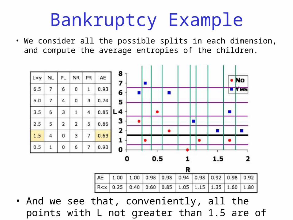
Bankruptcy Example• We consider all the possible splits in each dimension, and
compute the average entropies of the children.
• And we see that, conveniently, all the points with L not greater than 1.5 are of class 0, so we can make a leaf there.
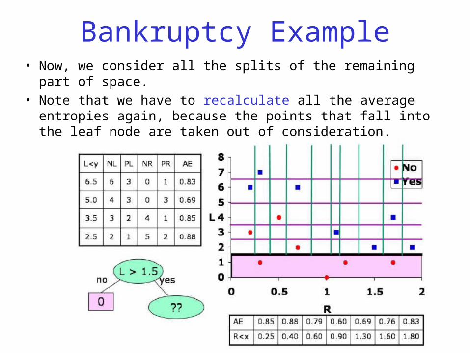
Bankruptcy Example• Now, we consider all the splits of the remaining part of space.
• Note that we have to recalculate all the average entropies again, because the points that fall into the leaf node are taken out of consideration.
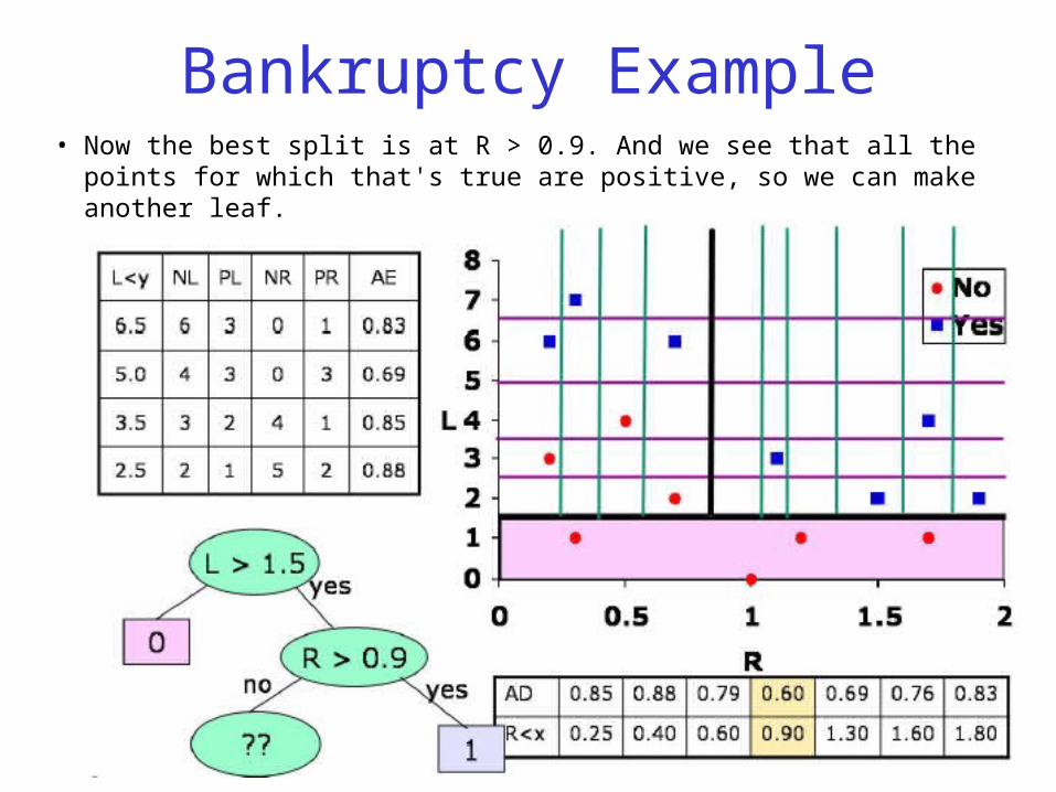
Bankruptcy Example• Now the best split is at R > 0.9. And we see that all the points
for which that's true are positive, so we can make another leaf.
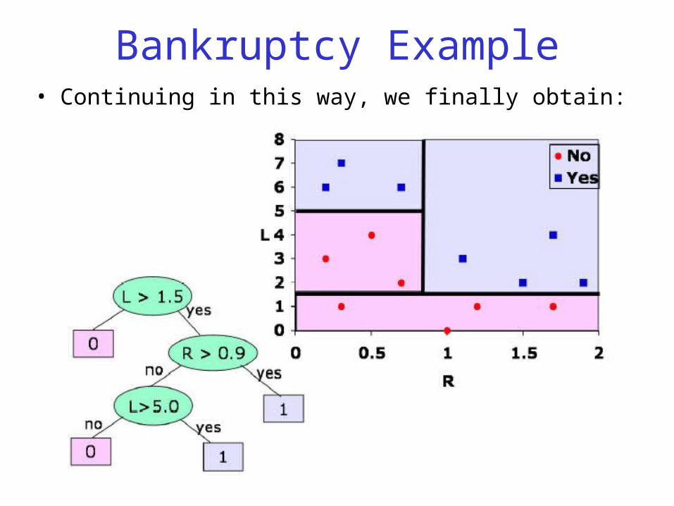
Bankruptcy Example• Continuing in this way, we finally obtain:
Rules: Covering• Strategy for generating a rule set directly is based on
covering.
• A rule “lhs then rhs” covers a data instance, if the tests in “lhs” are true for that instance.
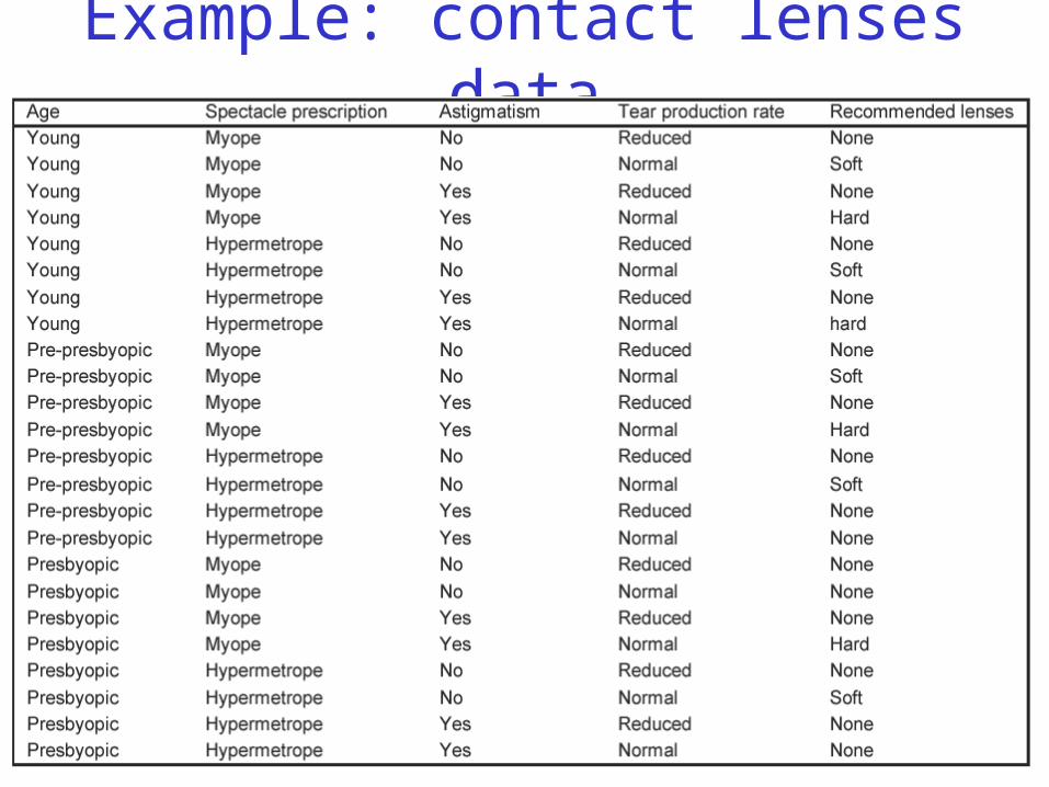
Example: contact lenses data
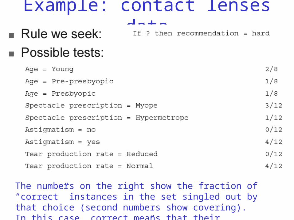
Example: contact lenses data
The numbers on the right show the fraction of “correct” instances in the set singled out by that choice (second numbers show covering).In this case, correct means that their recommendation is “hard.”
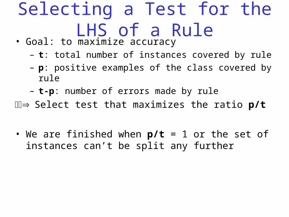
Selecting a Test for the LHS of a Rule• Goal: to maximize accuracy
– t: total number of instances covered by rule
– p: positive examples of the class covered by rule
– t-p: number of errors made by rule
Select test that maximizes the ratio p/t
• We are finished when p/t = 1 or the set of instances can’t be split any further
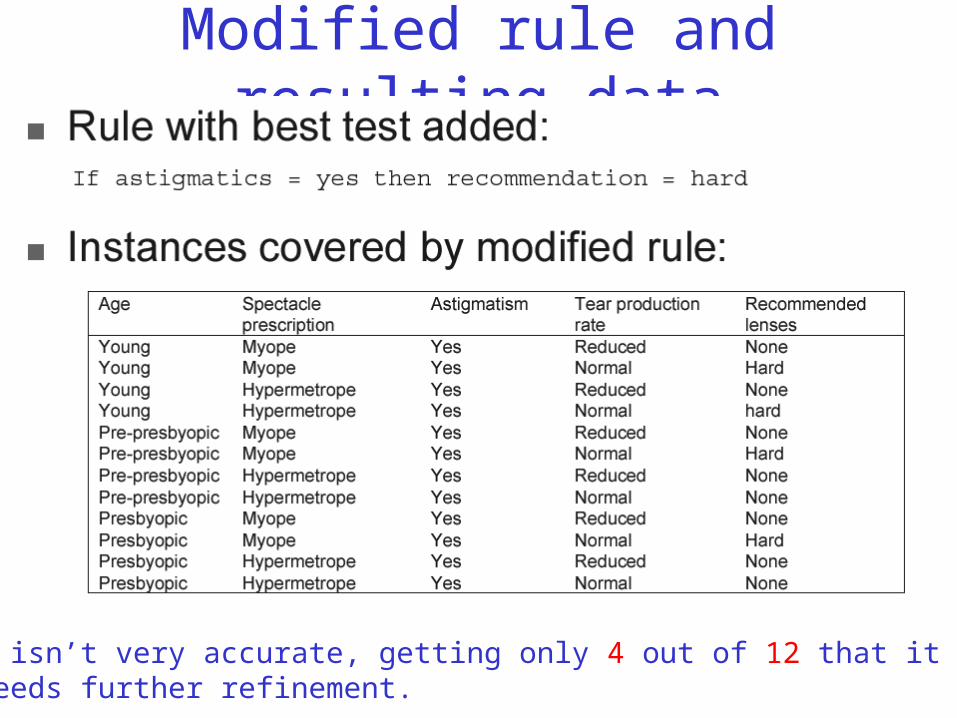
Modified rule and resulting data
The rule isn’t very accurate, getting only 4 out of 12 that it covers. So, it needs further refinement.
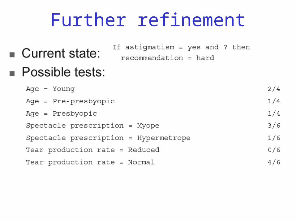
Further refinement
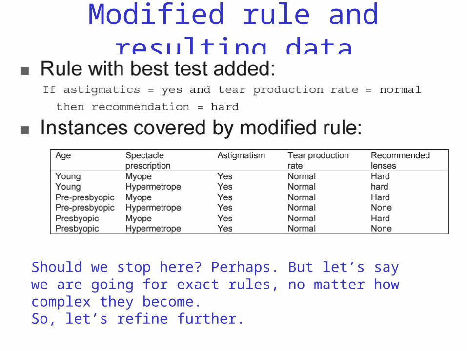
Modified rule and resulting data
Should we stop here? Perhaps. But let’s say we are going for exact rules, no matter how complex they become.So, let’s refine further.
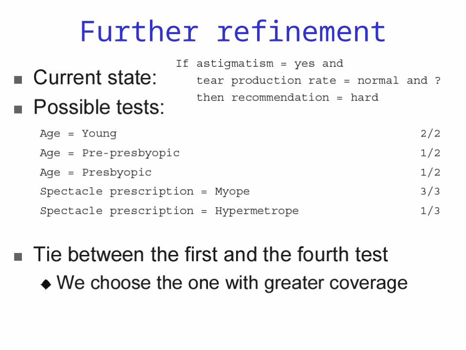
Further refinement
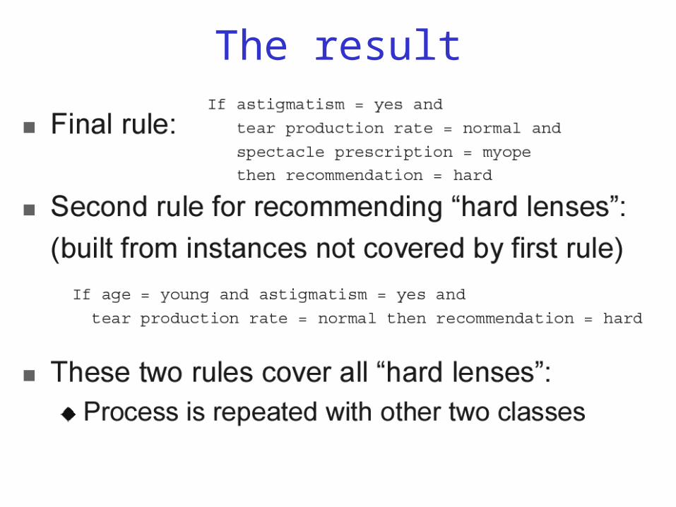
The result
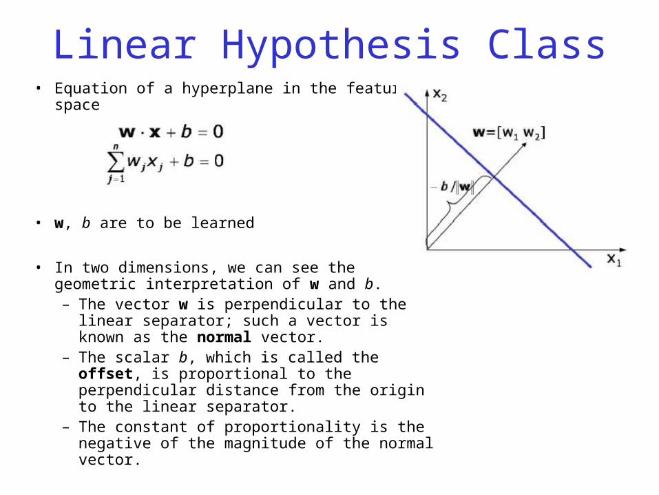
Linear Hypothesis Class• Equation of a hyperplane in the feature space
• w, b are to be learned
• In two dimensions, we can see the geometric interpretation of w and b. – The vector w is perpendicular to the linear
separator; such a vector is known as the normal vector.
– The scalar b, which is called the offset, is proportional to the perpendicular distance from the origin to the linear separator.
– The constant of proportionality is the negative of the magnitude of the normal vector.
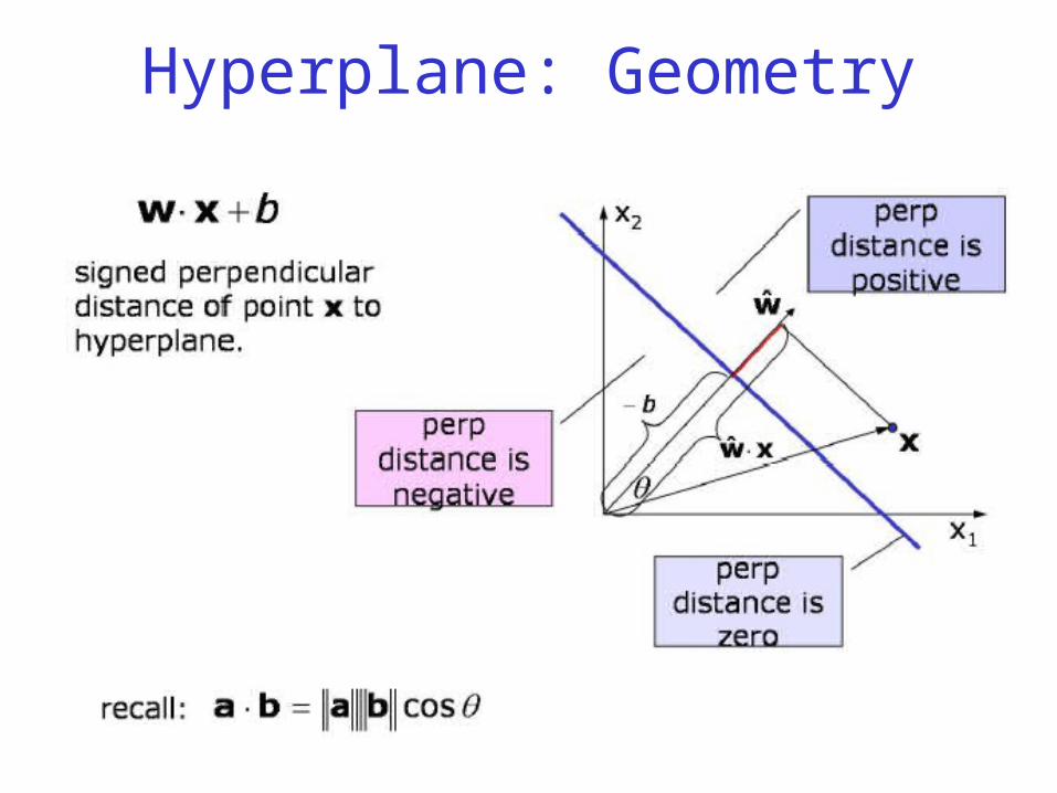
Hyperplane: Geometry
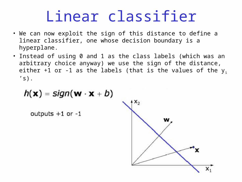
Linear classifier• We can now exploit the sign of this distance to define a linear
classifier, one whose decision boundary is a hyperplane.
• Instead of using 0 and 1 as the class labels (which was an arbitrary choice anyway) we use the sign of the distance, either +1 or -1 as the labels (that is the values of the yi ’s).
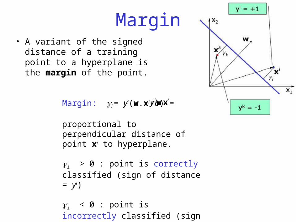
Margin• A variant of the signed
distance of a training point to a hyperplane is the margin of the point.
Margin: i = yi(w.xi+b) =
proportional to perpendicular distance of point xi to hyperplane.
i > 0 : point is correctly classified (sign of distance = yi)
i < 0 : point is incorrectly classified (sign of distance yi)
iiy xw
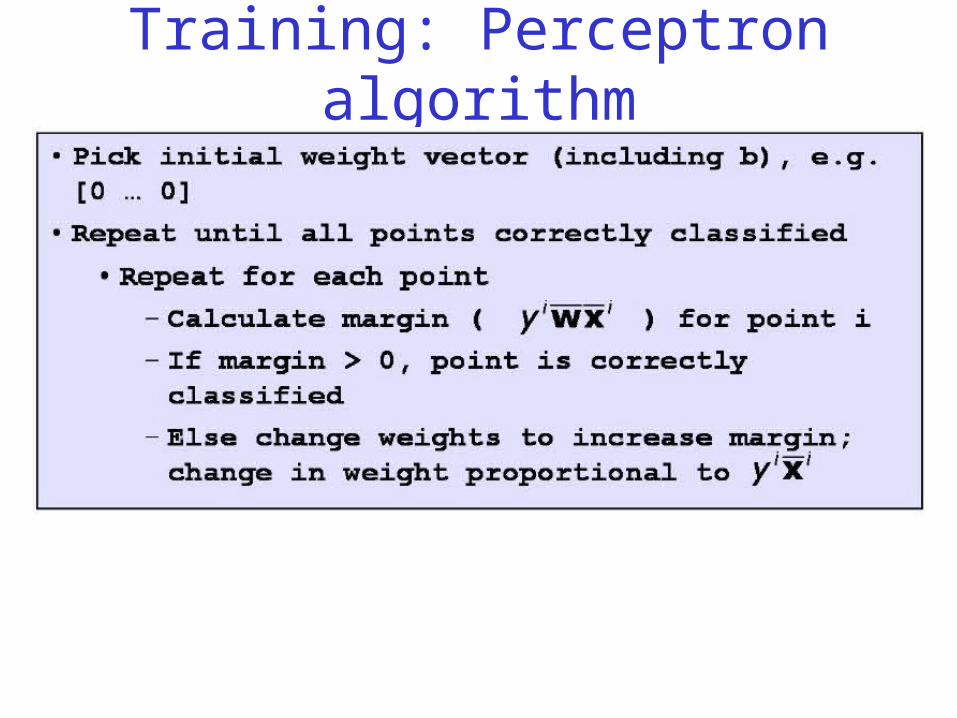
Training: Perceptron algorithm
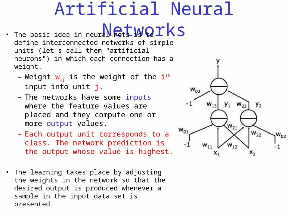
Artificial Neural Networks• The basic idea in neural nets is to define
interconnected networks of simple units (let's call them "artificial neurons") in which each connection has a weight.
– Weight wij is the weight of the ith input into unit j.
– The networks have some inputs where the feature values are placed and they compute one or more output values.
– Each output unit corresponds to a class. The network prediction is the output whose value is highest.
• The learning takes place by adjusting the weights in the network so that the desired output is produced whenever a sample in the input data set is presented.
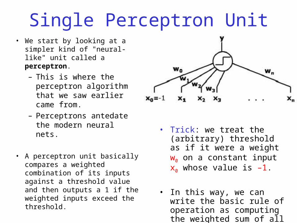
Single Perceptron Unit• We start by looking at a simpler
kind of "neural-like" unit called a perceptron.
– This is where the perceptron algorithm that we saw earlier came from.
– Perceptrons antedate the modern neural nets.
• A perceptron unit basically compares a weighted combination of its inputs against a threshold value and then outputs a 1 if the weighted inputs exceed the threshold.
• Trick: we treat the (arbitrary) threshold as if it were a weight w0 on a constant input x0 whose value is –1.
• In this way, we can write the basic rule of operation as computing the weighted sum of all the inputs and comparing to 0.
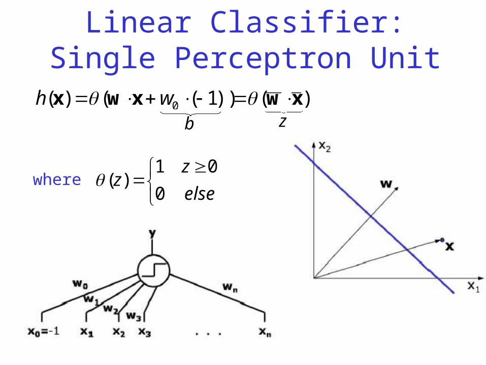
Linear Classifier: Single Perceptron Unit
)())1(()( 0 xwxwx whb z
where
else
zz
0
01)(
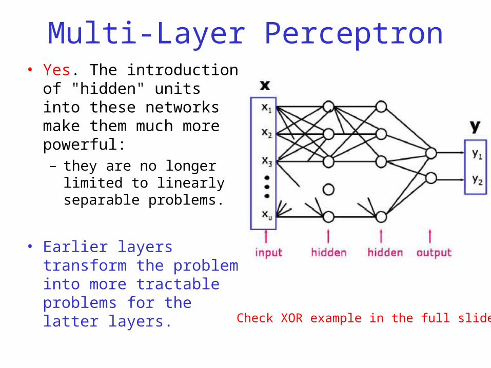
Multi-Layer Perceptron• Yes. The introduction of
"hidden" units into these networks make them much more powerful: – they are no longer limited to
linearly separable problems.
• Earlier layers transform the problem into more tractable problems for the latter layers.
Check XOR example in the full slides.
Multi-Layer Perceptron Learning• Any set of training points can be separated by a three-layer
perceptron network.
• “Almost any” set of points is separable by two-layer perceptron network.
• However, the presence of the discontinuous threshold in the operation means that there is no simple local search for a good set of weights; – one is forced into trying possibilities in a combinatorial way.
• The limitations of the single-layer perceptron and the lack of a good learning algorithm for multilayer perceptrons essentially killed the field for quite a few years.
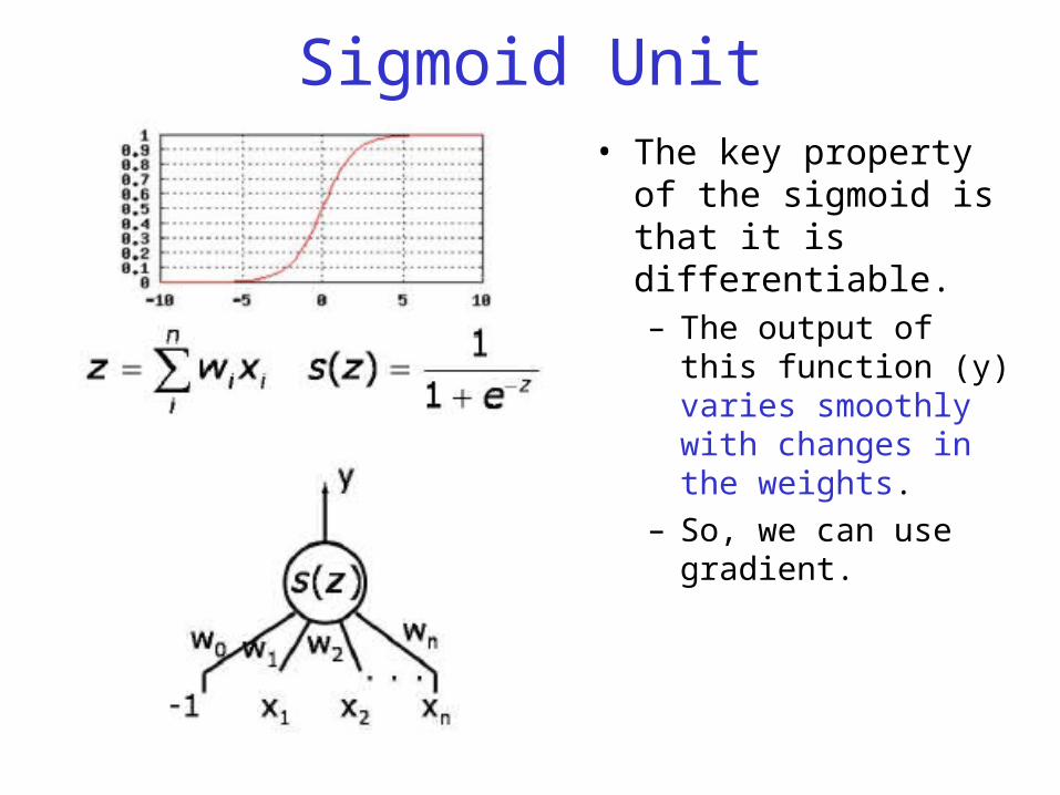
Sigmoid Unit• The key property of the
sigmoid is that it is differentiable. – The output of this
function (y) varies smoothly with changes in the weights.
– So, we can use gradient.
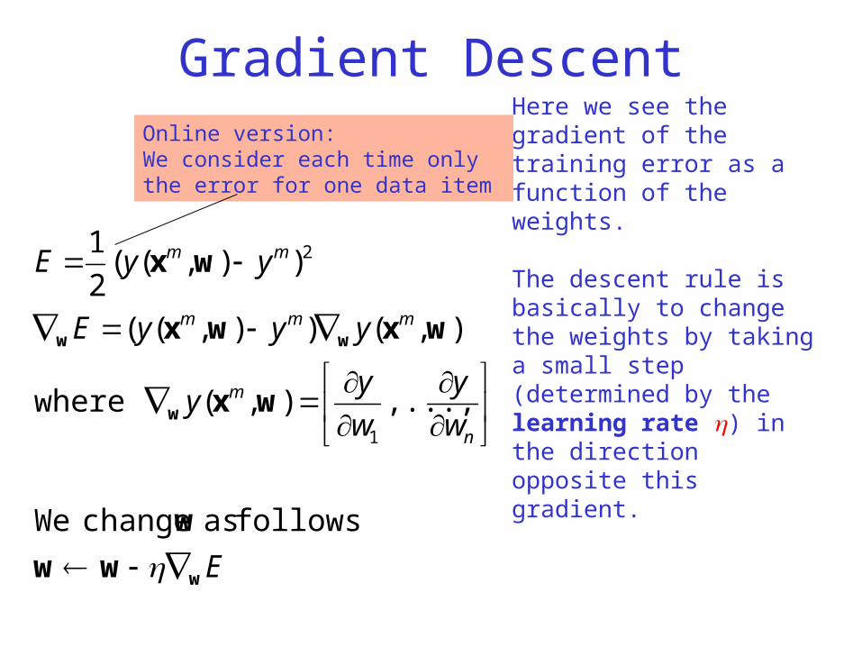
Gradient Descent
E
w
y
w
yy
yyyE
yyE
n
m
mmm
mm
w
w
ww
ww
w
wx
wxwx
wx
follows as change We
,...,),( where
),()),((
)),((2
1
1
2
Here we see the gradient of the training error as a function of the weights.
The descent rule is basically to change the weights by taking a small step (determined by the learning rate ) in the directionopposite this gradient.
Online version: We consider each time only the error for one data item
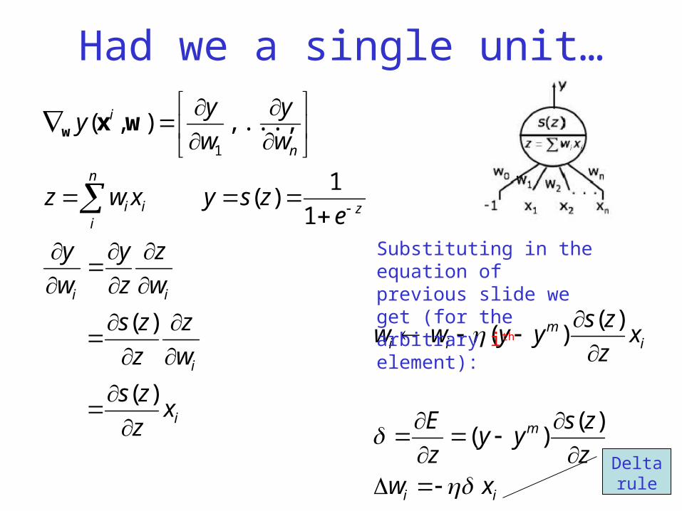
Had we a single unit…
i
i
ii
z
n
iii
n
i
xz
zs
w
z
z
zs
w
z
z
y
w
y
ezsyxwz
w
y
w
yy
)(
)(
1
1)(
,...,),(1
wxw
ii
m
im
ii
xwz
zsyy
z
E
xz
zsyyww
)()(
)()(
Delta rule
Substituting in the equation of previous slide we get (for the arbitrary ith element):
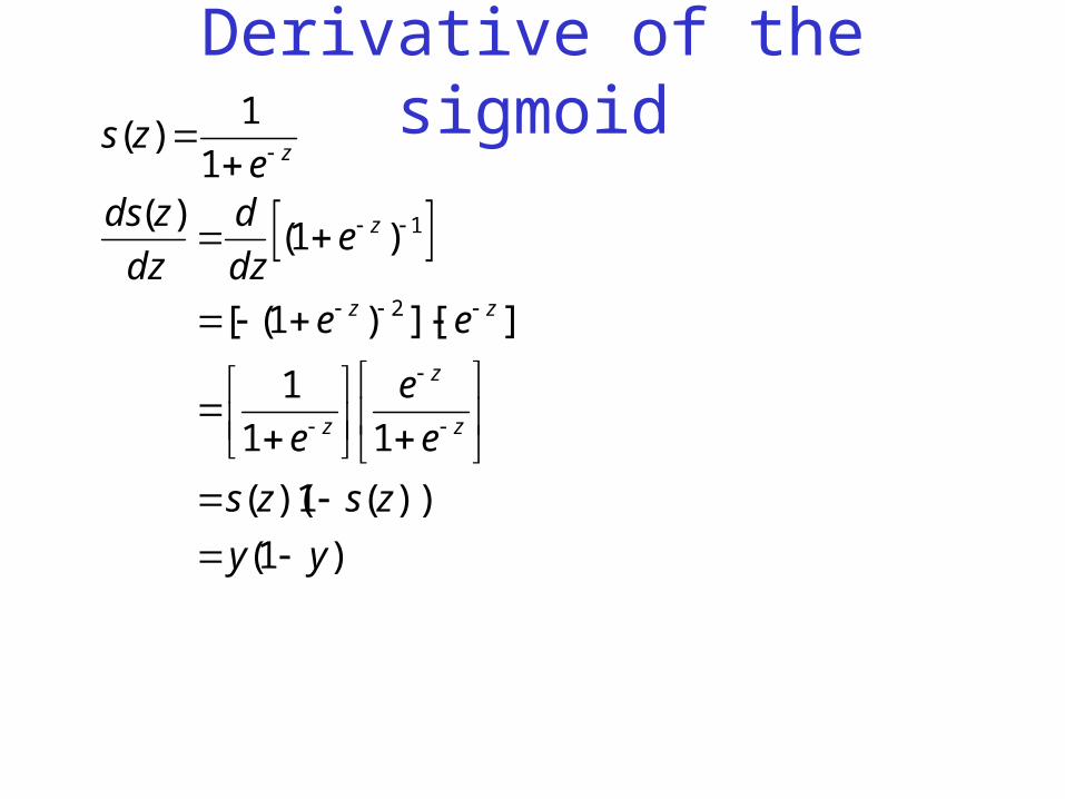
Derivative of the sigmoid
)1(
))(1)((
11
1
]][)1([
)1()(
1
1)(
2
1
yy
zszs
e
e
e
ee
edz
d
dz
zdse
zs
z
z
z
zz
z
z
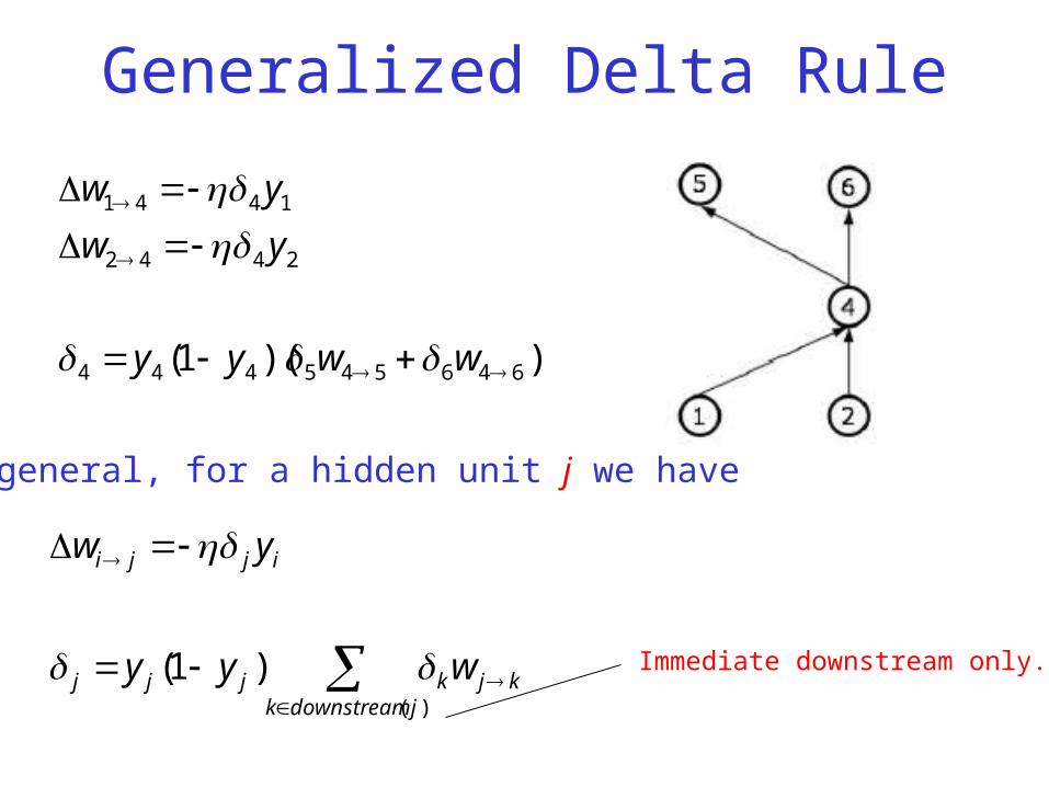
Generalized Delta Rule
))(1( 646545444
2442
1441
wwyy
yw
yw
)(
)1(jdownstreamk
kjkjjj
ijji
wyy
yw
In general, for a hidden unit j we have
Immediate downstream only.
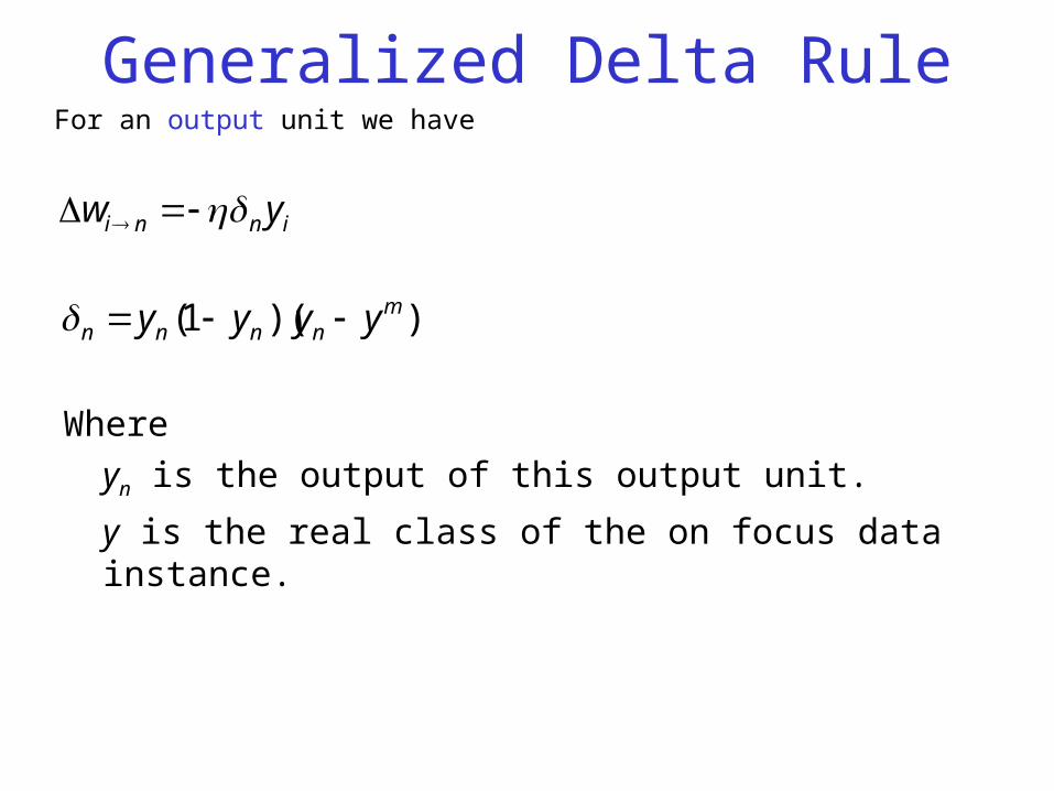
Generalized Delta RuleFor an output unit we have
))(1( mnnnn yyyy
inni yw
Where
yn is the output of this output unit.
y is the real class of the on focus data instance.
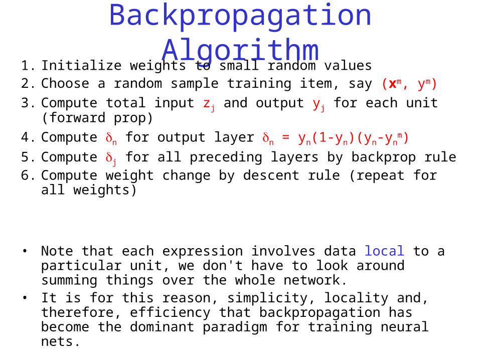
Backpropagation Algorithm1. Initialize weights to small random values2. Choose a random sample training item, say (xm, ym)
3. Compute total input zj and output yj for each unit (forward prop)
4. Compute n for output layer n = yn(1-yn)(yn-ynm)
5. Compute j for all preceding layers by backprop rule6. Compute weight change by descent rule (repeat for all weights)
• Note that each expression involves data local to a particular unit, we don't have to look around summing things over the whole network.
• It is for this reason, simplicity, locality and, therefore, efficiency that backpropagation has become the dominant paradigm for training neural nets.
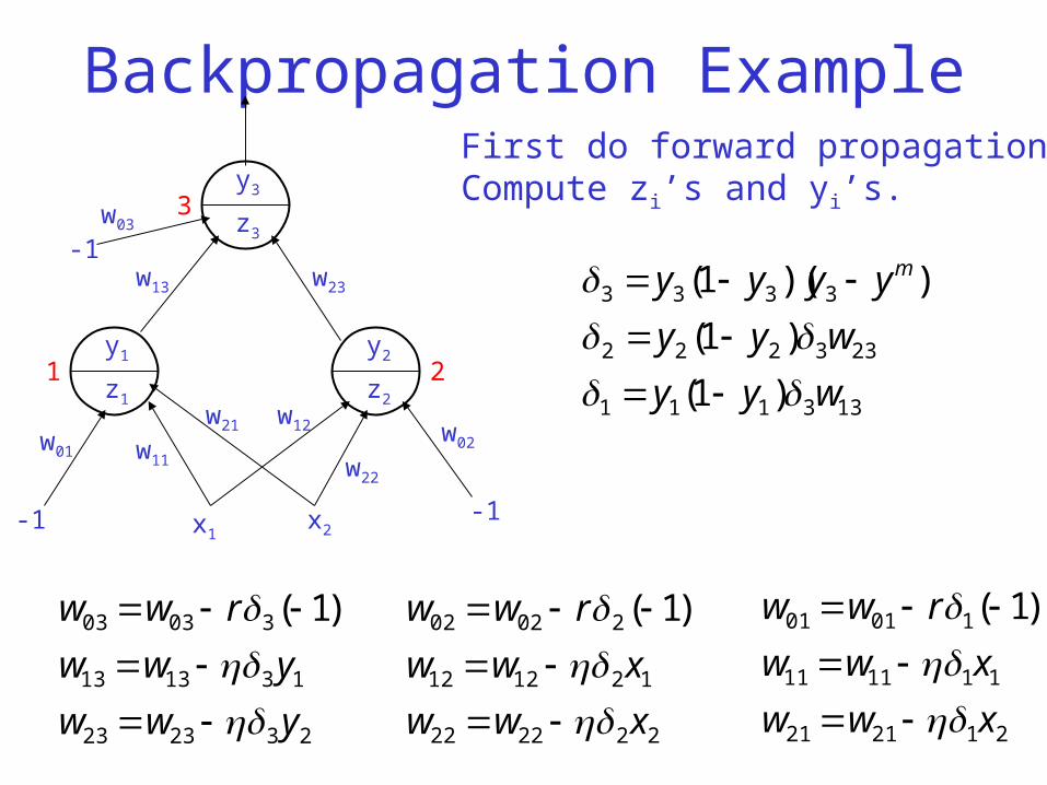
Backpropagation Example
y3
z3
y1
z1
y2
z2
1 2
3
-1 -1x1x2
w01
w03
w02w11 w22
w21
w13 w23
w12
-1
133111
233222
3333
)1(
)1(
))(1(
wyy
wyy
yyyy m
First do forward propagation:Compute zi’s and yi’s.
232323
131313
30303 )1(
yww
yww
rww
222222
121212
20202 )1(
xww
xww
rww
212121
111111
10101 )1(
xww
xww
rww