Review Article A Review on Migration Methods in B-Scan

Review ArticleA Review on Migration Methods in B-ScanGround Penetrating Radar Imaging

Caner Oumlzdemir Fevket Demirci Enes YiLit and Betuumll Yilmaz

Department of Electrical and Electronics Engineering Mersin University Ciftlikkoy 33343 Mersin Turkey

Correspondence should be addressed to Caner Ozdemir cozdemirmersinedutr

Received 14 March 2014 Accepted 5 May 2014 Published 10 June 2014

Academic Editor Fatih Yaman

Copyright copy 2014 Caner Ozdemir et alThis is an open access article distributed under the Creative Commons Attribution Licensewhich permits unrestricted use distribution and reproduction in any medium provided the original work is properly cited

Even though ground penetrating radar has been well studied and applied by many researchers for the last couple of decades thefocusing problem in the measured GPR images is still a challenging task Although there are many methods offered by differentscientists there is not any completemigrationfocusingmethod thatworks perfectly for all scenariosThis paper reviews the popularmigration methods of the B-scan GPR imaging that have been widely accepted and applied by various researchers The briefformulation and the algorithm steps for the hyperbolic summation the Kirchhoff migration the back-projection focusing thephase-shift migration and the 120596-119896 migration are presented The main aim of the paper is to evaluate and compare the migrationalgorithms over different focusing methods such that the reader can decide which algorithm to use for a particular application ofGPR Both the simulated and the measured examples that are used for the performance comparison of the presented algorithmsare provided Other emerging migration methods are also pointed out

1 Introduction

Ground penetrating radar (GPR) is remote sensing techniquethat can nondestructively sense and detect objects insidethe visually opaque environment or underneath groundsurface GPR has gained its fame thanks to its high reso-lution capability and applicability in numerous fields suchas detecting mines and unexploded ordinances findingwater leakages investigating archeological substances spot-ting asphaltconcrete cracks in highways searching buriedvictims after an earthquake or an avalanche and imagingbehind the wall for security applications [1ndash4] Depending onthe application different scanning schemes namely A-scanB-scan and C-scan are being employed [1] In the B-scanmeasurement situation a downward looking GPR antenna ismoved along a straight path on the top of the surfacewhile theGPR sensor is collecting and recording the scattered field atdifferent spatial positionsThis static measured data collectedat single point is called an A-scan [1]

The data collection in a typical GPR operation canbe either employed in the time domain by recording thescattered response of a time-domain pulse or in the frequencydomain by recording the frequency response of the scattered

field For the former case the two-dimensional (2D) space-time GPR image 119868(119909 119905) is attained by conveying a time-domain pulse towards the surface at consecutive distinctsynthetic aperture points For the latter case an inverseFourier transform (IFT) operation should be accommodatedto carry the collected data from the spatial-frequency domainto space-time GPR image In any case the depth resolutionis achieved by the transmitted signalrsquos frequency diversityThe resolution along the scanning direction is attained bythe synthetic processing of the received data collected atdifferent spatial points of the B-scan While a fine resolutionin the depth axis is usually easy to get by utilizing a wide-band transmitted signal the resolution along the scanningdirection is much harder to realize and requires special treat-ment On the other hand some specific GPR applications likepreservation tasks in ancient constructions or stone masonrystructures and detection of antipersonnel landmines forhumanitarian demining require high resolution images ofthe investigated structures or regions especially in the cross-range dimensions

In a typical space-time B-scan GPR image any scattererwithin the image region shows up as a hyperbola because of

Hindawi Publishing CorporationMathematical Problems in EngineeringVolume 2014 Article ID 280738 16 pageshttpdxdoiorg1011552014280738

2 Mathematical Problems in Engineering

the different trip times of the EM wave while the antennais moving along the scanning direction For this reasonthe resolution along the synthetic aperture direction depictsundesired low resolution features owing to the long tails ofthe hyperbola Therefore one of the most applied problemfor the B-scan GPR image is to transform (or to migrate) theunfocused space-time GPR image to a focused one show-ing the objectrsquos true location and size with correspondingEM reflectivity The common name for this task is calledmigration or focusing [5ndash18] In fact migrationmethods wereprimarily developed for processing seismic images [19] andthey were also applied to the GPR thanks to the likenessesbetween the acoustic and the electromagnetic wave equations[7ndash11] Kirchhoff rsquos wave-equation [5] and frequency-wavenumber (120596-119896) based [6 7] migration algorithms are widelyrecognized and employed The wave number domain focus-ing techniques for instance were first formulated for seismicimaging applications [7] and then adapted to the contempo-rary synthetic aperture radar (SAR) imaging practices [12ndash15] These algorithms are also named as seismic migration[12 13] and frequency-wave number (or 120596-119896) migration [16ndash18] by different researchers

In this work we present a brief review of the B-scanGPR migrationfocusing methods that are commonly usedby GPR research community Although we have done somepreliminary studies on the performance comparison of onlytwo GPR focusing algorithms earlier [20] by utilizing verylimited performance parameters in this paper we extendour studies to compare a total of five popular algorithms byassessing different aspects of these algorithms In Section 2we address the problem of migration together with the well-known exploding source concept In fact most migrationalgorithms make use of this concept as we shall explainin this work In Section 3 most popular and functionalmigration methods for the B-scan GPR imaging applicationsare reviewed For this purpose (i) hyperbolic summation(ii) Kirchhoff rsquos migration (iii) phase-shift migration (iv)frequency-wavenumber (or the 120596-119896) migration and (v)back-projection method are presented together with thedetailed algorithm steps In Section 4 the success and theperformance of these algorithms were compared to eachother by testing them over the simulated and the measuredB-scan GPR data Our main objective in this work is topresent a qualitative comparison of these popular and widelyused algorithms such that the reader can benefit from theperformance results over different parameters ranging fromresolution to computation time Section 5 is dedicated todiscussions and the conclusion

2 The Problem of MigrationFocusing

The common goal in a typical GPR image is to display theinformation of the spatial location and the reflectivity of anunderground object As illustrated in Figure 1 a single pointscatterer appears as a hyperbola in the space-time GPR imagefor themonostatic operation Since this is the expected imagepattern for the B-scan operation such information can bethought as sufficient if the main goal of the GPR application

is just to sense a pipe or comparable objects However theinformation about the scatterer including its depth its sizeand its EM reflectivity can be very important in most GPRapplications Therefore the hyperbola or dispersion in thespace-time B-scan GPR image ought to be converted to afocused one that demonstrates the objectrsquos factual locationand size together with its scattering amplitude A focusedor migrated image is gathered after the elimination of thishyperbolic type of diffraction or any other kind of dispersion[5ndash18]

21 Exploding Source Model Most of the migration methodsare based on the concept called exploding source model(ESM) In 1985 Claerbout [21] came with the clever idea ofthinking of the scattered field at the radar receiver as if itis originated from the source at the target location Insteadof assuming a two-way trip convention of the EM wavetherefore it is imagined that a fictitious source ldquoexploderdquo ata reference time of 119905 = 0 around the target location andsend EM wave to the receiver as illustrated in Figure 2 Thereal data collection scheme is shown in Figure 2(a) wherein fact the two-way propagation between the radar and theobject existsWhen theESM is utilized however the collecteddata is assumed to be originally radiated from the source onthe object Therefore one-way propagation is assumed in theESM depicted in Figure 2(b) Since the trip time of the EMwave would be half of the original problem the compensationshould be made for the velocity of the EM wave by justdividing it by two to have V

119898= V2 where V is the speed of

the EM wave within the medium of propagationThe migration using the ESM is essentially carried out by

applying these two actions

(i) the received signal is extrapolated back to explodingsource points

(ii) the migrated image is realized by forming the backextrapolated EM wave at the time of 119905 = 0

3 MigrationFocusing Methods

In this section we will briefly review the basic steps of themostly applied GPR algorithms namely the hyperbolic sum-mation the Kirchhoff migration the phase-shift migrationthe 120596-119896 (Stolt) migration and the back-projection focusingOther migration methods will also be mentioned at the endof this section

31 Hyperbolic (Diffraction) Summation In a typical GPRapplication the radar antenna collects the scattered or back-scattered EM wave from the air-to-ground interface andsubsurface objects together with many cluttering effectsmainly attributed to inhomogeneities within the ground Forthe idealistic case the phase of the scattered signal is directlyproportional to the trip time (or distance) that the EMwave possesses if the propagation medium is homogenousThe monostatic backscattered signal from a single point-likescatterer experiences different round-trip distances while theantenna is moving over the surface for the B-scan operation

Mathematical Problems in Engineering 3

Antenna

Sub-surface

1 2 Mminus1 M3

120576r

Air1205760

Cross range (syntheticaperture)

x

z

R1R2 R3

Space x

Time t

t3 = R3

t2 = R2

Object

(a)

(b)

t1 = R1

Figure 1 (a) Typical GPRmeasurement setup (B-scan) and (b) resultant space-time image that contains the well-known hyperbolic aliasing

120576r

Air 1205760

Object

Two-waypropagation

m = c

Subsurface

(a)

120576r

Antenna

Cross range (synthetic aperture)

Object

One-waypropagation

m = c2

Subsurface

(b)

Figure 2 Geometry for (a) B-scan GPR data collection scheme and (b) utilizing ldquoexploding source modelrdquo

For each static measurement along the B-scan axis one-dimensional (1D) range profile (or depth profile) of thesubsurface scene is obtained by taking the inverse Fouriertransform (IFT) of the frequency-diverse back-scattered sig-nal After putting all the depth profiles aside the 2D space-time (or space-depth) B-scan GPR image is obtained As theGPR antenna has a finite beamwidth any subsurface objectis illuminated for a finite length along the B-scan axis asdemonstrated in Figure 1 Therefore this object shows up as

a parabolic hyperbola in the space-time GPR image due todifferent trip distances of the EM wave between the radarand the illuminated scattering objectThe true location of theobject is in fact at the apex of this hyperbola

Let us assume a perfect point scatterer situated at (119909119900 119911119900)

in the 2D plane where 119909-axis corresponds to the scanningdirection and the 119911-axis is the depth as illustrated in Figure 1If the propagating medium is homogeneous the parabolichyperbola in the GPR image can be characterized by the


following equation when the radar is moving on a straightpath along 119883-axis Consider

R = radic1199112

119900+ (X minus 119909

119900)2

(1)

In the above equationX is the synthetic aperture vector alongthe B-scan and R represents the path length vector fromthe antenna to the scatterer Assuming that the resultant B-scan GPR image can be regarded as the contribution of finitenumber of hyperbolas that correspond to different points onthe object(s) below the surface the following methodologycan be applied tomigrate the defocused image structures thatis hyperbolas to the focused versions [22]

(i) For each pixel point (119909119894 119911119894) on the 2D original B-scan

space-depth GPR image matrix find the associatedhyperbolic template using (1) and trace all the pixelsunder this template

(ii) Record the image data for the traced pixels underthat template At this stage of the algorithm we have1D field data 119864

119904 whose length 119873 is the same asthe number of sampling points along the syntheticaperture 119883

(iii) Then calculate the root-mean-square (rms) of theentire energy contained inside this 1D complex fielddata as follows

rms at (119909119894 119911119894) =

radic(

1003816100381610038161003816Es10038161003816

10038161003816

210038161003816100381610038161003816(Es

)lowast10038161003816

100381610038161003816

2

)

119873

=

1

radic119873

119873

sum

119894=1

1003816100381610038161003816Esi1003816100381610038161003816

2

(2)

(iv) The calculated rms figure is recorded on the newimage matrix at the point (119909

119894 119911119894) This process is

reiterated until all pixels on the original GPR imageare passed through the algorithm

32 Kirchhoff rsquos Migration Kirchhoff rsquos migration (KM) alsoknown as reverse-time wave equationmigration is mathemat-ically equivalent to hyperbolic summationmethodwith somecorrecting factors included in the solution [22] InKirchhoff rsquosmigration procedure the aim is to find the solution to thefollowing scalarwave equation for thewave function120593(119909 119911 119905)

within the propagating medium

(

1205972

1205971199092

+

1205972

1205971199112

minus

1

V2119898

1205972

1205971199052

) 120593 (119909 119911 119905) = 0 (3)

Here V119898is the velocity of the EMwavewithin the propagating

medium and taken as V2 by utilizing the ldquoexploding sourcerdquoconcept The solution to this differential equation is availablefor the far-field approximation from the Kirchhoff integraltheorem [23] as

119875 (119909 119911 119905) =

1

2120587

int

infin

minusinfin

(

cos 120579

V119898

119877

sdot

120597

120597119905

119875 (119909 119911 119905 minus

119903

V119898

)) 119889119909 (4)

Here 120579 is the angle of the incident wave to the depth axis (119911)

and 119903 = ((119909 minus 119909119898

)2

+ 1199112

)

12 is the path from the target pointat (119909 119911) to the observation point at (119909

119898 0)

In KM method the following correction factors that arenot considered in the hyperbolic summation are accounted

(i) Compensation for the spherical spreading is takeninto account For this purpose a correction factor of1radicV119898

119903 is used for the 2D propagation of the EMwave whereas this factor becomes 1(V

119898119903) for the 3D

propagation(ii) The directivity factor cos 120579 is also considered This

factor corrects the diffraction amplitudes(iii) The phases and amplitudes of the wave are also

corrected The phase is corrected by 1205872 and 1205874

for 2D and 3D propagation cases respectively Theamplitude of the EM wave is corrected with a factorproportional to the square of the frequency for the2D propagation case and to the frequency for the 3Dpropagation case [23ndash25]

33 Phase-Shift Migration The phase-shift migration (PSM)method is first introduced and applied by Gazdag [6] Similarto Kirchhoff rsquos migration this method also utilizes the ESMconcept [26] In brief the algorithm iteratively puts a phase-shift to migrate the wave field to the exploding time of 119905 = 0

such that all the scattered waves are drawn back to object siteto have a focused image

The main aim of the PSM algorithm is to calculate thewave field at 119905 = 0 by extrapolating the downward (119911-directed) EM wave with the phase factor of exp(119895119896

119911119911)

The PSM algorithm can be briefly summarized via thefollowing steps

(i) First 2D measured raw dataset in frequency wave-number or (120596 119896

119909) domain is multiplied by a phase-shift

factor 119870 along the depth axis (or 119911-axis) as given below

119870 = 119890119895119896119911sdotΔ119911

(5)

This factor can also bewritten in terms of wave-number alongthe data collecting axis (119896

119909) as

119870 = exp (119895119896119911

sdot Δ119911)

= exp (119895radic1198962

minus 1198962

119909sdot Δ119911)

= exp(119895119896radic1 minus (

119896119909

119896

)

2

sdot Δ119911)

(6)

Putting 119896 = 120596V119898(where 120596 is the angular frequency and V

119898

is the speed of wave inside the propagationmedium) into (5)one can get

119870 = exp(119895

119908

Vsdot Δ119911radic1 minus (

V119898

sdot 119896119909

120596

)

2

) (7)

In the above equation the incremental depth parameter Δ119911

is proportional to the time sampling interval Δ119905 of the input


data via Δ119911 = V119898

sdot Δ119905 After this modification the final formof the phase-shift factor becomes

119870 = exp(119895119908 sdot Δ119905radic1 minus (

V119898

sdot 119896119909

120596

)

2

) (8)

2D measured raw dataset 119864119904

(120596 119896119909) is multiplied by 119870 along

the depth axis for the time steps of Δ119905(ii) By utilizing the ESM concept the imaging task is

accomplished by taking the inverse Fourier transform (IFT)of the 119864

119904

(120596 119896119909) after selecting the time variable as Δ119905 = 0

Therefore only single FT operation is required at one point(when Δ119905 = 0) for the focused image

After updating the factor 119870 for every value of Δ119905 and 120596we have the data in 3D (120596 119896

119909 119896119911) domain as

1198641199041015840

(120596 119896119909 119896119911) = 119870 sdot 119864

119904(120596 119896119909) (9)

The new dataset 1198641199041015840

(120596 119896119909 119896119911) is summed up along the

frequency axis and indexed for different values of Δ119905 as

119864119904

(119896119909 119896119911 119905) = sum

119908

1198641199041015840

(120596 119896119909 119896119911) (10)

(iii) Setting Δ119905 = 0 and taking the 2D IFT with respect to119896119909and 119896119911 the focused the image in the (119909 119911) domain can be

obtained as given below119864119904

(119909 119911) = IFT 119864119904

(119896119909 119896119911) (11)

34 Frequency-Wavenumber (Stolt) Migration Frequency-wavenumber (120596-119896) migration also known as Stolt migrationor the 119891-119896 migration utilizes the ESM idea and the scalarwave equation [7] The algorithm behind the frequency-wavenumber method works faster than the previously pre-sented migration methods The 120596-119896 migration method hasproven to be working well for the constant-velocity propa-gation mediums [6 7] The solution of the 120596-119896 migrationcan be rewritten to be the same as the solution of theKirchhoffmigration [18] Below is the brief explanation of thealgorithm

The algorithm begins with the 3D scalar wave equationfor thewave function120593(119909 119910 119911 119905)within the constant-velocitypropagation medium

(

1205972

1205971199092

+

1205972

1205971199102

+

1205972

1205971199112

minus

1

V2119898

1205972

1205971199052

) 120593 (119909 119910 119911 119905) = 0 (12)

In the Fourier space spatial wave-numbers and the frequencyof operation are related with the following equation

1198962

119909+ 1198962

119910+ 1198962

119911= 1198962

=

1205962

V2119898

(13)

Stratton [27] demonstrated that any given wave function canbe written as the summation of infinite number of plane wavefunctions say 119864(119896

119909 119896119910

120596) as

120593 (119909 119910 119911 119905) = (

1

2120587

)

32

∭

infin

minusinfin

119864 (119896119909 119896119910

120596)

times 119890minus119895(119896119909119909+119896119910119910+119896119911119911minus120596119905)

119889119896119909119889119896119910

119889120596

(14)

For the GPR operation the scattered field is taken to bemeasured on the 119911 = 0 plane above the surface Whencarefully treated the above equation offers a Fourier trans-formpair where 119890(119909 119910 119905) can be regarded as the time-domainmeasured field on the 119911 = 0 plane Consider

120593 (119909 119910 0 119905) ≜ 119890 (119909 119910 119905)

= (

1

2120587

)

32

∭

infin

minusinfin

119864 (119896119909 119896119910

120596)

times 119890minus119895(119896119909119909+119896119910119910minus120596119905)

119889119896119909119889119896119910

119889120596

(15)

It is very important to notice that this equation desig-nates a 3D forward FT relationship between 119890(119909 119910 119905) and119864(119896119909 119896119910

120596) for the negative values of time variable 119905 Thenthe inverse FT can be dually defined in the following way

119864 (119896119909 119896119910

120596) = (

1

2120587

)

32

∭

infin

minusinfin

119890 (119909 119910 119905)

times 119890119895(119896119909119909+119896119910119910minus120596119905)

119889119909 119889119910 119889119905

(16)

Afterwards we nowuse the ESM to focus the image by setting119905 = 0 in (15) and using

119864 (119896119909 119896119910

120596) = 119890119895119896119911119911

119864 (119896119909 119896119910

120596 119911 = 0) (17)

Therefore one can get the time-domain measured field via

119890 (119909 119910 119911 0) = (

1

2120587

)

32

∭

infin

minusinfin

119864 (119896119909 119896119910

120596)

times 119890minus119895(119896119909119909+119896119910119910+119896119911119911)

119889119896119909119889119896119910

119889120596

(18)

The above equation presents a focused image Howeverthe data in (119896

119909 119896119910

120596) domain should be transformed to(119896119909 119896119910

119896119911) domain to be able to use the FFT Therefore a

mapping procedure from 120596 domain to 119896119911domain is required

for fast processing The relationship between the 120596- and -119896119911

and 119889120596- and -119889119896119911can be easily obtained from (13) as

120596 = V119898

(1198962

119909+ 1198962

119910+ 1198962

119911)

12 (19a)

119889120596 =

V2119898

119896119911

120596

119889119896119911 (19b)

Substituting these equations into (18) one can obtain thefollowing

119890 (119909 119910 119911) = (

1

2120587

)

32

∭

infin

minusinfin

V2119898

119896119911

120596

119864119898

(119896119909 119896119910

119896119911)

times 119890minus119895(119896119909119909+119896119910119910+119896119911119911)

119889119896119909119889119896119910

119889119896119911

(20)

Here 119864119898

(119896119909 119896119910

119896119911) is the mapped version of the original

data 119864(119896119909 119896119910

120596) After this mapping the new data set does


AntennaSynthetic aperture

Soil

h

120576r

Air 1205760

Imaging scene

Scenecenter

(x0 z0)

rm

um

120579m

x

x

z

z

Range(depth)

(xm zm)

Scenec eS ncentere erc t

(((xxx0 zzzz0)))

rmmrr

uumm

120579120579120579mm

xxxx

zz

Figure 3 The B-scan geometry of the 2D monostatic GPR application

not lie on the uniform grid due to nonlinear feature of thetransformationTherefore an interpolation procedure shouldalso be applied to be able to use the FFT for fast processing ofthe collected dataset Equation (20) suggests a well-focusedimage of the subsurface region that may contain a finitenumbers of scatterers Since the FFT routine is utilized theGPR image in the 120596-119896 migration is obtained quite fast It isalso important to express that the mapped dataset is scaledby the factor of V2

119898119896119911120596 This scaling is sometimes called the

ldquoJacobian transformation from 120596 to 119896119911rdquo

The above focusing equation is valid for the 3D GPRgeometry or the C-scan problem Inmost subsurface imagingproblems however the raw data is collected in 2D space thatis space-time (space-depth) or space-frequency Thereforethe focusing equation in (20) can be easily reduced to 2DB-scan GPR problem in the space-depth domain via thefollowing equation

119890 (119909 119911) = (

1

2120587

) ∬

infin

minusinfin

V2119898

119896119911

120596

119864119898

(119896119909 119896119911)

times 119890minus119895(119896119909119909+119896119911119911)

119889119896119909119889119896119911

(21)

35 Back-Projection BasedMigration The last category of theGPR focusing algorithms is based on the tomographic prin-ciples used in medical imaging and collectively termed as theback-projection (BP) algorithms Since its first formulationfor the 2Dmonostatic SAR processing [28] the BP algorithmhas gathered an increasing interest in radar communitythanks to its distinct features that are proved to be veryuseful for various SAR imaging applications For examplethe algorithm does not require a straight and uniformlysampled synthetic scan aperture due to its serial processingnature More clearly each 1D range profiles are seriallyprocessed and spread or back-projected over the entire 2Dimage independentlyThis sequential processingmeans ldquoreal-timerdquo operation capability and hence the imaging process

can begin before acquiring the entire synthetic aperture dataFurthermore the specific subsections of the region to beimaged can be easily selected to investigate these subsectionsmore closely In applications where the approximate locationof the target is known a priori the detailed image of the regionaround this target can be easily formed by the algorithm

Before briefly explaining the algorithm let us firstconsider the B-scan monostatic GPR geometry shown inFigure 3 A radar antenna situated at a height of ℎ fromthe ground transmits a frequency-diverse waveform at eachdistinct point 119898 along the synthetic axis The relative per-mittivity of the subsurface medium is denoted by 120576

119903and

the reflectivity function of the scatterers is represented by119890(119909 119911) The instantaneous position of the antenna (119909

119898 119911119898

) isdefined by a unit vector um pointing from the scene centertowards this location The corresponding view-angle 120579

119898is

defined as the angle between the unit vector um and the depthaxis 119911 Assuming a stepped-frequency continuous waveform(SFCW) transmission the back-scattered signal at a specificobservation angle can be written as

119878120579119898

[119896119903] = ∬

infin

minusinfin

119890 (119909 119911) exp (minus119895119896119903119903119898

) 119889119909 119889119911 (22)

where 119896119903is the wavenumber defined for the two-way prop-

agation as 119896119903

= 4120587119891V 119891 is the frequency V is the speed ofthe propagation and 119903

119898is the range from the instantaneous

antenna location (119909119898

119911119898

) to the points (1199090 1199110) within the

imaging scene The range profile of the illuminated scenecan be obtained by employing 1D IFT to (22) and can bemathematically conveyed as

119904120579119898

(119903) equiv IFT 119878120579119898

(119896119903)

= ∬

infin

minusinfin

119890 (119909 119911) 120575 (119903119898

minus 119903) 119889119909 119889119911

(23)

which is nothing but the Radon transform of the scene


The derivation of the BPA [29] begins with the imple-mentation of IFT of the scattering function 119890(119909 119911) written inCartesian coordinates as

119890 (119909 119911) = ∬

infin

minusinfin

119864 (119896119909 119896119911) exp [119895 (119896

119909119909 + 119896119911119911)] 119889119896

119909119889119896119911 (24)

where 119864(119896119909 119896119911) is the 2D FT of 119890(119909 119911) Equation (24) can be

reformed to be rewritten in the polar coordinates (119896119903 120579119898

) asfollows

119890 (119909 119911) = int

120587

minus120587

int

infin

0

119864 (119896119903 120579119898

) exp (119895119896119903119903119898

) 119896119903119889119896119903119889120579119898

(25)

Now the projection-slice theorem [30] can be used to relatethe targetrsquos FT119864(119896

119909 119896119911) to the collectedmeasured data 119878

120579(119896119903)

For the 2D problem the theorem essentially states that 1D FTof the projection at the angle 120579 represents the slice of the 2DFT of the projected (original) scene at the same angle thatis 119878120579(119896119903) = 119864(119896

119903 120579) Therefore the sampled representation

of 119864(119896119909 119896119911) can be obtained from the FT of the projections

119878120579(119896119903) measured at several observation aspects By the help

of this principle (25) becomes

119890 (119909 119911) = int

120587

minus120587

[int

infin

0

119878120579119898

(119896119903) exp (119895119896

119903119903119898

) 119896119903119889119896119903] 119889120579119898

(26)

The bracketed integral term in (26) can be regarded as the1D IFT of a function 119876

120579119898

(119896119903) = 119878

120579119898

(119896119903)119896119903calculated at

119903119898 Defining 119902

120579119898

(119903) as the IFT of this function (26) can berepresented as

120588 (119909 119911) = int

120587

minus120587

119902120579119898

(119903119898

) 119889120579119898

(27)

Equation (27) is the final focused image of the 2D filteredback-projection algorithm For the SFCW system the execu-tion of the algorithm can be summarized as follows

(1) Preallocate an image matrix of zeros 119890(119909 119911) to holdthe values of the scene reflectivity

(2) Multiply the acquired spatial-frequency data 119878120579119898

(119896119903)

with 119896119903

(3) Take 1D IFT of the result to obtain 119902120579119898

(119903) whichrepresents the filtered version of the range profile119904120579119898

(119903)

(4) For each pixel position in the image data evaluate thecorresponding range value 119903

119898and acquire its 119902

120579119898

(119903119898

)

value by the help of an appropriate interpolationmethod

(5) Iteratively add interpolated data values to 119890(119909 119911)

(6) Repeat the above steps from 2 to 5 to cover all theobservation angles 120579

119898

36 Some Other Methods In addition to the above men-tioned common migration methods there are many othertechniques that have been introduced and studied by differentGPR researchers Fisher et al [31] applied reverse-timemigration procedure for GPR profiles Capineri et al [32]applied a technique based on Hough transformation to theB-scan GPR data to attain better resolved images of pipestructures Leuschen and Plumb [9] and Morrow and vanGenderen [33] realized back-propagation procedures thatrely on finite difference time-domain (FDTD) reverse-timefocusing methods to resemble the focusing matter in GPRimages

4 Performance Comparison of the Algorithms

Performance of the algorithms is evaluated by the help offollowing various parameters that are resolution integratedsidelobe ratio signal to clutter ratio and computation speed

Resolution GPR measurement can provide fine resolutionsboth in depth and azimuth resolutions The term depth(range) corresponds to the line of sight distance from theradar to the target to be imaged The term azimuth (trans-verse range cross range) is used for the dimension that isperpendicular to range or parallel to the radarrsquos along-trackaxis [34] The depth resolution is defined as an ability ofthe radar equipment to separate two reflecting objects on asame line of sight but at different ranges from the antennaAnd the azimuth resolution can be defined as a capability ofthe separation of two reflecting objects on the same rangesbut different aspects from the radar In GPR operation thehigh resolution in depth is obtained by utilizing a transmittedsignal of wideband Fine azimuth resolution is achieved bycoherently processing the targetrsquos electromagnetic scatteringmeasured at different aspects while the radar is moving alonga straight path However the measured resolutions after thepostprocessing are dependent on the focusing ability of themigration algorithmThat is why the resolution performanceof the algorithms is tested bymeasuring theminus4 dB contours ofa point scatterer (whose coordinate is 119909 = 0m and 119911 = 15m)in the resultant images of simulations Normally algorithmswith better focusing abilities are expected to produce lowerresolved images

Integrated Sidelobe Ratio (ISLR) Since ISLR is defined asthe ratio of the total energy within the sidelobes to thepeak energy of the main lobe [35] it can be regarded as animportant parameter when assessing the focusing abilities ofmigration algorithms [36] Based on Sanchezrsquos definition ofILSR it is the ratio of the minus3 dB width of the main lobe to therest of the energy within all lobesTherefore the ISLR of a 2Dimage function 119868(119909 119910) can be formulated as follows

ISLR = 10log10

(

intminus3 dB 119868119889119909

1015840

1198891199101015840

int

+infin

minusinfin

11986811988911990910158401198891199101015840

minus intminus3 dB 119868119889119909

10158401198891199101015840

) (28)

where intminus3 dB 119868119889119909

1015840

1198891199101015840 is the energy within the minus3 dB width of

the main lobe and int

+infin

minusinfin

1198681198891199091015840

1198891199101015840 is the total energy


Table 1 Performances of focusing algorithms over different parameters for the simulated experiments

Algorithm Computation time (s) Depth resolution (cm) Azimuth resolution (cm) ISLR (dB)HSA 4632 678 12 minus1315KMA 937270 543 4 minus1217PSA 213 870 10 minus1302120596-119896A 041 630 4 minus1275BPA 429 770 58 minus613

Signal to Clutter Ratio (SCR) Signal to clutter ratio (SCR) isalso a crucial parameter when evaluating the quality of thefocusing ability In a well-focused image the clutternoiselevel should bemuch lower than the signal level to have awell-contrasted image The SCR can be defined as the ratio of thereceived target signal power to the received clutter power asshown below

SCR = 10log10

(

119875tar119875tot minus 119875tar

) (29)

where 119875tar is the received target signal power and 119875tot is thetotal power within the image

Computation Speed The processing time of the computationof the algorithms can be crucial if the GPR applicationrequires processing of vast data such as scanning and cleaninga minefield

41 Comparison over Simulation The migration algorithmswere first tested through an imaging simulation performed inMATLAB Considering the classical B-scan geometry shownin Figure 4 the subsurface was assumed to have a completelyhomogeneous soil medium structure (ie constant-velocitymedium)with a dielectric constant of 24Themedium is alsoassumed to be nonmagnetic that is 120583

119903= 1 The monostatic

operation was considered and the minus3 dB beamwidth of theantenna was assumed to be large enough such that all targetsto be imaged fall inside the beam for the whole aperture withconstant antenna gain The electric field data of the isotropicpoint scatterers with locations depicted in Figure 4 were thencollected along a straight path ranging from 119909 = minus25mto 119909 = 25m and with 2 cm steps At each spatial pointthe frequency response of the subsurface was acquired forthe 125GHzndash375GHz frequency range that was uniformlysampled at 168 points Therefore 251 times 168 spatial-frequencyB-scan data 119864(119909 119891) were generated for the investigatedsceneThe frequency data were subsequently preprocessed byapplying a Hanning window for sidelobe control and 4 timeszero padding for interpolation purposes

Figure 5(a) shows the raw unfocused B-scan image sim-ply formed by applying a 1D inverse Fourier transform tothe collected data 119864(119909 119891) As expected the target reflectionsare observed as hyperbolas with different intensities andcurvature slopes To collapse these hyperbolic signatures atthe apex of the hyperbolas the migration algorithms wereapplied and the corresponding obtained results were given inFigures 5(b)ndash5(f) As a quick interpretation it can be noticedfrom all images that the scattering mechanisms are almostconcentrated around the exact locations of the targets

Antenna

Soil

1 Mminus1 M

L

120576r

Air 1205760

(0 15) m

Synthetic aperture xDepth z

Origin

(0 45) m

(minus15 3) m (15 3) m

Figure 4 Simulation geometry of the B-scan imaging example

To compare the performances of the algorithms Table 1lists the success merits of the algorithms including thedepth resolution the azimuth resolution the ISLR and thecomputational time By looking at the resolution outcomes inboth depth and azimuth direction KM and 120596-119870 algorithmsseem to provide better resolved images On the other handKMA is the worst in terms of computation time while 120596-119896Ais the fastest among all others In terms of the ISLR BPA issuperior to any other algorithm by providing a sharp ISLRthat is at least 6 dB better than the others When comparingall parameters one can conclude that the BPA and120596-119896A seemto have a little bit better in terms of the migration ability

When the resultant focused images of these algorithmsare visually compared in Figure 5 the KM the BPA andthe 120596-119896A look more successful than others as the resultsof the HSA and PSA expose some image degradations Ifthose well-localized images of Figures 5(c) 5(e) and 5(f) arecompared some minor differences can even be discernedbetween each other For example the target reflections in theBP migrated image have more regular pattern and also havestronger intensities Also the images for the KM and the 120596-119896A have some relatively higher sidelobe levels around the topand bottom targets Additionally if the image for the 120596-119896A iscarefully checked (see Figure 5(e)) the depth of the bottomtarget is also shown to be mapped to 119911 = 4mwhich indicatesa little deviation from its true value of 119911 = 45m

By evaluating the GPR images in Figure 5 we can com-pare the focusing algorithms against each other as followsWhile the 120596-119896A may experience some problems in imagingdeep targets with low reflectivities successful imaging of


Unfocused image0

1

2

3

4

5

6

Synthetic aperture x (m)

Dep

thz

(m)

minus2 minus1 0 1 2minus40

minus35

minus30

minus25

minus20

minus15

minus10

minus5

0

(a)

Hyperbolic (diffraction) summation0

1

2

3

4

5

6


Dep

thz

(m)


minus35

minus30

minus25

minus20

minus15

minus10

minus5

0

(b)

Kirchoffc migration0

1

2

3

4

5

6


Dep

thz

(m)


minus35

minus30

minus25

minus20

minus15

minus10

minus5

0

(c)

Phase-shift migration0

1

2

3

4

5

6


Dep

thz

(m)


minus35

minus30

minus25

minus20

minus15

minus10

minus5

0

(d)

0

1

2

3

4

5

6


Dep

thz

(m)


minus35

minus30

minus25

minus20

minus15

minus10

minus5

0Frequency-wavenumber (w-k) migration

(e)

Back-projection-based focusing0

1

2

3

4

5

6


Dep

thz

(m)


minus35

minus30

minus25

minus20

minus15

minus10

minus5

0

(f)

Figure 5 Simulation results for the minus40 dB dynamic range



1

2

3

4

5

6


Dep

thz

(m)


minus35

minus30

minus25

minus20

minus15

minus10

minus5

0

(a)


1

2

3

4

5

6


Dep

thz

(m)


minus35

minus30

minus25

minus20

minus15

minus10

minus5

0

(b)

Figure 6 Results of the hyperbolic summation and Kirchhoff rsquos migration algorithms for a decreased frequency sampling interval (iefrequency bandwidth 119861 = 45GHz with 302 sampling points)

shallow targets can be problematic for the KM Secondlythe images for the HSA and the PSA look considerablypoorer than those of the other algorithms This can be seenfrom the significantly defocused image that correspondsto PSA (see Figure 5(d)) This image also has some extraundesired scattering features such as blurring and spreadingOn the other hand the image for the HSA exhibits a majordegradation only around the uppermost target The othertargets are observed to be almost well focused

To comprehend the sources of abovementioned defo-cusing effects for these two algorithms another simulationwas performed by utilizing different simulation parametersFor this simulation the total number of frequency sampleswas increased to 302 points The bandwidth was then cor-respondingly changed to 119861 = 45GHz to satisfy the sameunambiguous range of the previous simulation that is 65mCorresponding results for the simulation are demonstrated inFigure 6 It is shown from the Figure 6(a) that the HSA is notaffected from the variation of the sampling points along thedepth directionThemigrated image is similar to the previousresult given in Figure 5(b) except for the definite resolutionenhancement thanks to wider bandwidth In any case HSAis shown to have difficulty only in providing a reasonablerepresentation of the uppermost target along the spatialdirection Although this aliasing is also somewhat observedfor the deeper targets they can also be regarded as wellfocusedwithin the dynamic range ofminus40 dB As stated beforethis spatial aliasing for the shallower target is also slightlyobserved in the result of the KA as given in Figure 5(c)Thusnoting the similarities between these algorithms this fact canbe assumed to stem from the characteristics of thesemethodsNevertheless this spatial aliasing can be avoided by utilizingdifferent implementations such as the ones that incorporate

more points along a hyperbolic trajectory rather than usinga single point during integration

The PSA result seen in Figure 6(b) conversely showsdrastic improvement when compared to the previous oneshown in Figure 5(d) All of the four scatterers are shownto be well localized for the increased value of the frequencysampling points This notable change can be attributed tothe algorithmsrsquo iterative processing nature along the depthdirection Since the PSA first records the data at the surfaceand repeatedly multiply this data with a phase factor foreach downward range points the short sampling intervalswould result in better quality images Hence this syntheticexample illustrates that the PSA is highly sensitive to theemployed frequency sampling interval Lastly due to thealgorithmic similarities between the PSA and the 120596-119896A thecorresponding images given in Figures 6(b) and 5(e) areshown to have similar distortion patterns especially seen atthe bottom of these images

Finally the computational efficiency of the algorithms istested by looking at the simulation runtime and the requiredmemory during implementation Based on our evaluationthe computational efficiency of the algorithms is listed fromthe best to the worst as follows the 120596-119896A the PSA the BPAthe HSA and the KM

42 Comparison over Measurement The performance of thefocusing algorithms is also tested by the help of measureddata sets For this purpose two different experiments wereconducted to better understand the differences between thefocusing capabilities of the algorithms for real datasetsTheseexperiments were conducted by the help of the AgilentE5071B ENA Vector Network Analyzer (VNA) that can


Unfocused image0

02

04

06

08

1

12


Dep

thz

(m)

minus40

minus35

minus30

minus25

minus20

minus15

minus10

minus5

0

minus06 minus04 minus02 0 02 04 06

(a)


02

04

06

08

1

12


Dep

thz

(m)

minus40

minus35

minus30

minus25

minus20

minus15

minus10

minus5

0


(b)

Kirchhoff s migration0

02

04

06

08

1

12


Dep

thz

(m)

minus40

minus50

minus60

minus30

minus20

minus10

0


(c)


02

04

06

08

1

12


Dep

thz

(m)

minus40

minus35

minus30

minus25

minus20

minus15

minus10

minus5

0


(d)

0

02

04

06

08

1

12


Dep

thz

(m)

minus40

minus35

minus30

minus25

minus20

minus15

minus10

minus5

0


Frequency-wavenumber (w-k) migration

(e)


02

04

06

08

1

12


Dep

thz

(m)

minus40

minus35

minus30

minus25

minus20

minus15

minus10

minus5

0


(f)

Figure 7 Results for the real soil Experiment 1 Note the different dynamic range (ie minus60 dB) for the Kirchhoff migration result


X synthetic apertureZ depth

Origin

Metal plateLocation (x z) = (48 20) cm

Metal pipeLocation (x z) = (1 18) cmSize 7 cm diameter 33 cm length

Plastic bottleLocation (x z) = (minus47 15) cmSize 6 times 6 times 25 cm W D L

Figure 8 Geometric representation of the targets used in Experiment 2

generate SFCW signals within the frequency range of 08ndash85 GHz In both experiments a C-band double-ridged pyra-midal rectangular horn antenna was used as a monostatictransceiver

421 Experiment Number 1 In the experiment we haveconstructed a test bed by building a big wooden poolwith a size of 190 cm times 100 cm times 80 cm and filled it withhomogeneous and dry sand material The dielectric constantof the sand was measured to be almost constant around24 for the frequency range between 1GHz and 8GHz It isalso assumed that the sand material has the unit magneticpermeability for the frequencies of operation Two cylindricalmetal rods with different sizes were selected as targets in thescene The thin rod with 45 cm in diameter and 45 cm inlength was buried at (119909 = minus12 cm 119911 = 65 cm) and a thick rodwith 6 cm in diameter and 32 cm in length was buried at (119909 =

18 cm 119911 = 75 cm) A B-scanmeasurement was accomplishedby moving the antenna along the perpendicular direction ofthe target axes and by spanning a synthetic aperture lengthof 119871 = 134m sampled at 63 spatial points The steppedfrequency response of the medium was then obtained for abandwidth of 08ndash45GHz that was uniformly sampled at 751points

After collecting the data the classical space-depth B-scan GPR image is obtained as shown in Figure 7(a) fromwhich the unfocused target signatures can be clearly seenThegoverning scattering mechanism from air-ground boundaryis also easily detected around at 119911 = 40 cm and seenthroughout the entire synthetic aperture Then we apply theabove presented migration algorithms in aiming at gettinga better focused image The resultant migrated images aredisplayed in Figures 7(b) to 7(f) wherein the target responsesare seen to be more localized around their correct locationsTo better compare the algorithms against each other allresultant focused images were displayed within the samedynamic range of minus60 dB The focusing performance of allalgorithms seems to be very similar to each other as thetails (or the sidelobes) of the targetsrsquo images are comparabledispersion features In terms of the image contrast the 120596-119896A and the PSA outperforms the BPA the HSA and theKM as it can be clearly deducted from the images For thisexperiment the numerical noise generated by the iterativeimplementation of the BPA seems to be very high when

Figure 9 A scene from real soil measurements

compared to other algorithms In fact the real data containsinfinite number of scatterers (with high or low reflectivities)under the ground it seems that the BPA is more sensitive toreflectivity amplitude than the others

422 Experiment Number 2 In the second experiment thealgorithms were tested under a more heterogeneous soil inanother test bed of the indoor environment The targets wereselected as a water-void target a metal pipe and a metal platewhose sizes and burial locations were as depicted in Figure 8The synthetic aperture length was set to 134 cm for a totalof 68 discrete points and the frequency was changed from08GHz to 5GHz for 501 discrete points A picture duringthe experiment is presented in Figure 9

After collecting the data the raw image obtained bytaking the IFT of the measured back-scattering data is shownin Figure 10(a) As expected the image is unfocused aroundthe buried objects After applying the migration algorithmsthe focused images of the three buried objects are acquiredas seen in Figures 10(b) to 10(f) For this experiment verysimilar features were observed as in the case of the firstexperiment Again focusing performances of the algorithmsare alike as the sidelobe contours of targetrsquos images are com-parable The contrast performances of the images also yield


Unfocused image0

02

04

06

08

1

12minus06 minus04 minus02 0 02 04 06

minus40

minus35

minus30

minus25

minus20

minus15

minus10

minus5

0


Dep

thz

(m)

(a)


02

04

06

08

1


minus40

minus45

minus50

minus35

minus30

minus25

minus20

minus15

minus10

minus5

0


Dep

thz

(m)

(b)


02

04

06

08

1


minus40

minus50

minus60

minus30

minus20

minus10

0


Dep

thz

(m)

(c)


02

04

06

08

1


minus40

minus35

minus30

minus25

minus20

minus15

minus10

minus5

0


Dep

thz

(m)

(d)

0

02

04

06

08

1


minus40

minus35

minus30

minus25

minus20

minus15

minus10

minus5

0


Dep

thz

(m)


(e)


02

04

06

08

1


minus40

minus35

minus30

minus25

minus20

minus15

minus10

minus5

0


Dep

thz

(m)

(f)

Figure 10 Results for the real soil Experiment 2 Note the different dynamic ranges (ie minus50 and minus60 dB) for the hyperbolic summation andKirchhoff rsquos migration results


Table 2 Performances of focusing algorithms over different param-eters for the measured experiments

Experiment number 1 results Experiment number 2 resultsSCR (dB) Time (s) SCR (dB) Time (s)

HSA minus627 1112 minus1248 761KMA minus455 572380 minus947 267630PSA minus541 1399 minus1040 374120596-119896A minus566 057 minus992 034BPA minus448 175 minus901 219

similar finding as we found in the first experiment Againthe 120596-119896A and the PSA produce more quality images whencompared to other three algorithms As the final commentsthe BPA seems to have problems again when dealing withreal-world data as it produces significant numerical noise asit can be seen from Figure 10(f)

Table 2 summarizes the performance of the presented fivedifferent algorithms in terms of processing time and the SCRover the conducted measurements In assessing the speedof the algorithms we observe similar performances as inthe case of the simulation results that are listed in Table 1Again 120596-119896A is the fastest one and the BPA is the second bestwhile the KMA is the worst If we look at the SCR resultsthe clutter suppression ability of BPA is the best while theothers demonstrate moderate performances when comparedto BPA

5 Conclusion and Discussions

In this paper we have reviewed and compared fundamentalalgorithms that are used to focus the B-scan GPR data bypresenting the algorithm steps Namely the hyperbolic sum-mation the Kirchhoff migration the phase-shift migrationthe frequency-wavenumber (120596-119896) migration and the back-projection based migration algorithms have been explainedand applied to both the simulation and the measurementexperiments Based on the results obtained from the simu-lated and measured images we have the following remarksfor the investigated migration algorithms

(i) The HSA is conceptually very simple and thereforeit is very easy to implement On the other handnumerous hyperbolic template vectors should beapplied for every pixel in the image which in turnis an expensive process in terms of the computationtime If the image size is relatively big then the wholeprocess of calculating the energy under the hyperbolictemplates of every pixel may take a very long timeAlthough the focusing ability of the algorithm is notas good as the 120596-119896A and the BPA the measurementresults have showed that focusing success of the HSAalso has some merit as it can be seen from theconstructed GPR images Also the HSA produce faircontrast images when compared to others

(ii) Although KM is conceptually similar to HSA thealgorithm is based on the scalar wave equation andit corrects the amplitude and the phases of some

parameters such as spherical spreading anddirectivitythat are not taken in to account in HSA Thereforethe results obtained by KM are a little bit better thanthe ones with HSA that can also be seen from theresulted images This is of course at the price of alonger simulation time The improvement obtainedby this amplitude correction can be clearly observedin Figures 7(c) and 10(c) to be compared to the imagesin Figures 7(b) and 10(b) The targets with smallerreflectivity are more visible in the images obtainedwith KM By looking at both the simulation andthe measurement results KMA seems to provide thebest resolution figures when compared to other fouralgorithms

(iii) The PSA utilizes the ESM concept and iteratively triesto add phase-shifts to migrate the wave field to theexploding time of 119905 = 0 The algorithm uses theadvantage of FFT therefore it is much faster than theabovementioned algorithms The PSArsquos performancein terms of computation time focusing and imagequality is modest when compared to others

(iv) Stolt migration algorithm (or the 120596-119896A) also makesuse of the ESM concept and the scalar wave equationfor the scattered field It can be shownmathematicallythat the 120596-119896A provides the same solution set asin the case of KM The 120596-119896A tries to constitutea 3D Fourier transform relationship between theimage at the object space and the collected scat-tered field Before applying the FFT routine a map-ping procedure from frequency-wavenumber domainto wavenumber-wavenumber domain is necessaryAlthough this mapping procedure may slow downthe execution time of the algorithm it is still fastthanks to the FFT step This study suggests that thefocusing performance and the image quality feature ofthe 120596-119896A are the best among all five algorithms Thealgorithm is also fast when compared to HSA KMand BPA

(v) As the BPA is not conceptually as simple as HSA orKM the implementation of the algorithm is morecomplex On the other hand the BPA is much fasterthan these two algorithms since it takes and acts onthe data as a block Therefore it requires less com-putation resources when compared to HSA or KMThis study has showed that the BPA is quite fast and itsfocusing ability is also very good This can be viewedfrom both the simulated and the measured imagesand from the listed tables where BPA is the best foralmost all the focusing parameters One drawbackof the BPA is due to its vulnerability to numericalnoise The algorithm produces comparably highernoise floor when compared to other four algorithmsThis situation may cause resultant images of the lowreflectivity targets to lie under the exaggerated noisefloor level Therefore such targets may not be imagedwithin selection of dynamic range for the imagedisplay


Conflict of Interests

The authors declare that there is no conflict of interestsregarding the publication of this paper

Acknowledgment

Thiswork is supported by the Scientific andResearchCouncilof Turkey (TUBITAK) under Grant no EEEAG-104E085

References

[1] D J Daniels Surface-Penetrating Radar IEEE Press 1996[2] L Peters Jr J J Daniels and J D Young ldquoGround penetrating

radar as a subsurface environmental sensing toolrdquo Proceedingsof the IEEE vol 82 no 12 pp 1802ndash1822 1994

[3] S Vitebskiy L Carin M A Ressler and F H Le ldquoUltra-wideband short-pulse ground-penetrating radar simulationand measurementrdquo IEEE Transactions on Geoscience andRemote Sensing vol 35 no 3 pp 762ndash772 1997

[4] L Carin N Geng M McClure J Sichina and L NguyenldquoUltra-wide-band synthetic-aperture radar for mine-fielddetectionrdquo IEEE Antennas and Propagation Magazine vol 41no 1 pp 18ndash33 1999

[5] W A Schneider ldquoIntegral formulation formigration in two andthree dimensionsrdquo Geophysics vol 43 no 1 pp 49ndash76 1978

[6] J Gazdag ldquoWave equation migration with the phase-shiftmethodrdquo Geophysics vol 43 no 7 pp 1342ndash1351 1978

[7] R H Stolt ldquoMigration by Fourier transformrdquo Geophysics vol43 no 1 pp 23ndash48 1978

[8] E Baysal D D Kosloff and J W C Sherwood ldquoReverse timemigrationrdquo Geophysics vol 48 no 11 pp 1514ndash1524 1983

[9] C J Leuschen and R G Plumb ldquoA matched-filter-basedreverse-timemigration algorithm for ground-penetrating radardatardquo IEEE Transactions on Geoscience and Remote Sensing vol39 no 5 pp 929ndash936 2001

[10] K Gu G Wang and J Li ldquoMigration based SAR imagingfor ground penetrating radar systemsrdquo IEE Proceedings RadarSonar and Navigation vol 151 no 5 pp 317ndash325 2004

[11] J SongQH Liu P Torrione andLCollins ldquoTwo-dimensionaland three-dimensionalNUFFTmigrationmethod for landminedetection using ground-penetrating radarrdquo IEEE Transactionson Geoscience and Remote Sensing vol 44 no 6 pp 1462ndash14692006

[12] C Cafforio C Prati and F Rocca ldquoFull resolution focusingof Seasat SAR images in the frequency-wave number domainrdquoInternational Journal of Remote Sensing vol 12 no 3 pp 491ndash510 1991

[13] C Cafforio C Prati and F Rocca ldquoSAR data focusing usingseismic migration techniquesrdquo IEEE Transactions on Aerospaceand Electronic Systems vol 27 no 2 pp 194ndash207 1991

[14] A S Milman ldquoSAR imaging by 120596-k migrationrdquo InternationalJournal of Remote Sensing vol 14 no 10 pp 1965ndash1979 1993

[15] H J Callow M P Hayes and P T Gough ldquoWavenumberdomain reconstruction of SARSAS imagery using single trans-mitter and multiplereceiver geometryrdquo Electronics Letters vol38 no 7 pp 336ndash338 2002

[16] A Gunawardena andD Longstaff ldquoWave equation formulationof synthetic aperture radar (SAR) algorithms in the time-spacedomainrdquo IEEE Transactions on Geoscience and Remote Sensingvol 36 no 6 pp 1995ndash1999 1998

[17] Z Anxue J Yansheng W Wenbing and W Cheng ldquoExper-imental studies on GPR velocity estimation and imagingmethod using migration in frequency-wavenumber domainrdquoin Proceedings of the 5th International Symposium on AntennasPropagation and EMTheory (ISAPE rsquo00) pp 468ndash473 BeijingChina 2000

[18] C Gilmore I Jeffrey and J LoVetri ldquoDerivation and com-parison of SAR and frequency-wavenumber migration withina common inverse scalar wave problem formulationrdquo IEEETransactions on Geoscience and Remote Sensing vol 44 no 6pp 1454ndash1461 2006

[19] J Gazdag and P Sguazzero ldquoMigration of seismic datardquo Pro-ceedings of the IEEE vol 72 no 10 pp 1302ndash1315 1984

[20] COzdemir S Demirci and E Yigit ldquoA review on themigrationmethods in B-scan ground penetrating radar imagingrdquo in Pro-ceedings of the Progress in Electromagnetics Research Symposium(PIERS rsquo12) pp 789ndash793 Kuala Lumpur Malaysia March 2012

[21] J F Claerbout Imaging the Earthrsquos Interior Blackwell ScientificPublications 1985

[22] C Ozdemir S Demirci E Yigit and A Kavak ldquoA hyperbolicsummation method to focus B-scan ground penetrating radarimages an experimental study with a stepped frequency sys-temrdquo Microwave and Optical Technology Letters vol 49 no 3pp 671ndash676 2007

[23] O Yilmaz Seismic Data Processing Society of ExplorationGeophysicists 1987

[24] D S Jones The Theory of Electromagnetism Pergamon PressNew York NY USA 1964

[25] P M Morse and H Feshbach Methods of Theoretical PhysicsMcGraw-Hill New York NY USA 1953

[26] I Lecomte S-E Hamran and L-J Gelius ldquoImproving Kirch-hoff migration with repeated local plane-wave imaging ASAR-inspired signal-processing approach in prestack depthimagingrdquo Geophysical Prospecting vol 53 no 6 pp 767ndash7852005

[27] J A Stratton ElectromagneticTheory McGraw-Hill New YorkNY USA 1941

[28] D C Munson Jr J D OrsquoBrien and W K Jenkins ldquoAtomographic formulation of spotlight-mode synthetic apertureradarrdquo Proceedings of the IEEE vol 17 no 8 pp 917ndash925 1983

[29] J L Bauck and W K Jenkins ldquoTomographic processing ofspotlight-mode synthetic aperture radar signals with compen-sation for wavefront curvaturerdquo in Proceedings of the Interna-tional Conference on Acoustics Speech and Signal Processing(ICASSP rsquo88) vol 2 pp 1192ndash1195 New York NY USA 1988

[30] R Mersereau and A Oppenheim ldquoDigital reconstruction ofmultidimensional signals from their projectionsrdquo Proceedings ofthe IEEE vol 62 no 10 pp 1319ndash1338 1974

[31] E Fisher G A McMechan A P Annan and S WCosway ldquoExamples of reverse-time migration of single-channel ground- penetrating radar profilesrdquoGeophysics vol 57no 4 pp 577ndash586 1992

[32] L Capineri P Grande and J A G Temple ldquoAdvanced image-processing technique for real-time interpretation of ground-penetrating radar imagesrdquo International Journal of ImagingSystems and Technology vol 9 no 1 pp 51ndash59 1998

[33] I L Morrow and P A van Genderen ldquo2D polarimetricbackpropagation algorithm for ground-penetrating radar appli-cationsrdquoMicrowave and Optical Technology Letters vol 28 pp1ndash4 2001


[34] C Ozdemir Inverse Synthetic Aperture Radar Imaging withMatlab Algorithms John Wiley amp Sons Hoboken NJ USA2012

[35] A Martinez and J L Marchand ldquoSAR image quality assess-mentrdquo Revista de Teledeteccion no 2 pp 1ndash7 1993

[36] E Yigit S Demirci C Ozdemir and M Tekbas ldquoShort-rangeground-based synthetic aperture radar imaging performancecomparison between frequency-wavenumber migration andback-projection algorithmsrdquo Journal of Applied Remote Sensingvol 7 2013

Submit your manuscripts athttpwwwhindawicom

Hindawi Publishing Corporationhttpwwwhindawicom Volume 2014

MathematicsJournal of


Mathematical Problems in Engineering

Hindawi Publishing Corporationhttpwwwhindawicom

Differential EquationsInternational Journal of

Volume 2014

Applied MathematicsJournal of


Probability and StatisticsHindawi Publishing Corporationhttpwwwhindawicom Volume 2014

Journal of


Mathematical PhysicsAdvances in

Complex AnalysisJournal of


OptimizationJournal of


CombinatoricsHindawi Publishing Corporationhttpwwwhindawicom Volume 2014

International Journal of


Operations ResearchAdvances in

Journal of


Function Spaces

Abstract and Applied AnalysisHindawi Publishing Corporationhttpwwwhindawicom Volume 2014

International Journal of Mathematics and Mathematical Sciences


The Scientific World JournalHindawi Publishing Corporation httpwwwhindawicom Volume 2014


Algebra

Discrete Dynamics in Nature and Society



Decision SciencesAdvances in

Discrete MathematicsJournal of


Volume 2014 Hindawi Publishing Corporationhttpwwwhindawicom Volume 2014

Stochastic AnalysisInternational Journal of


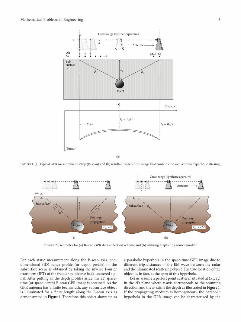
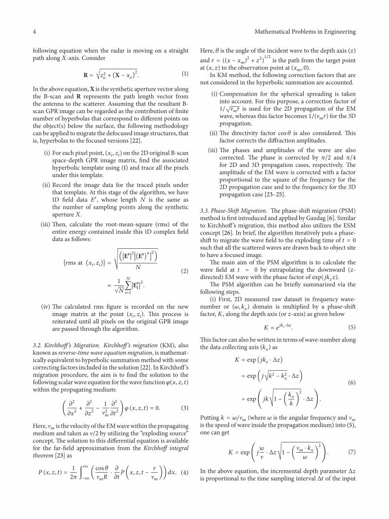
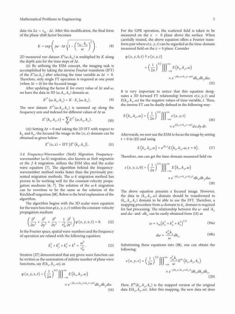
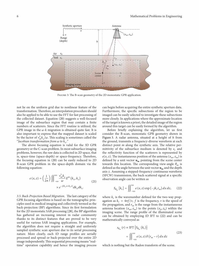
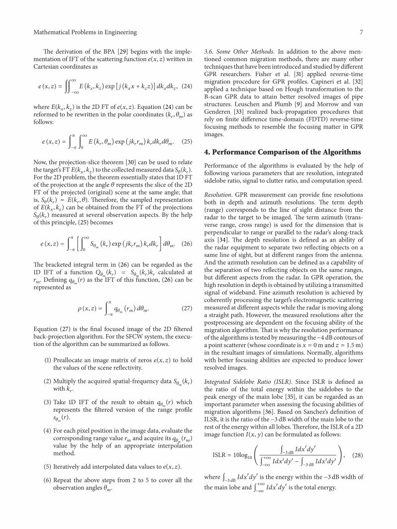
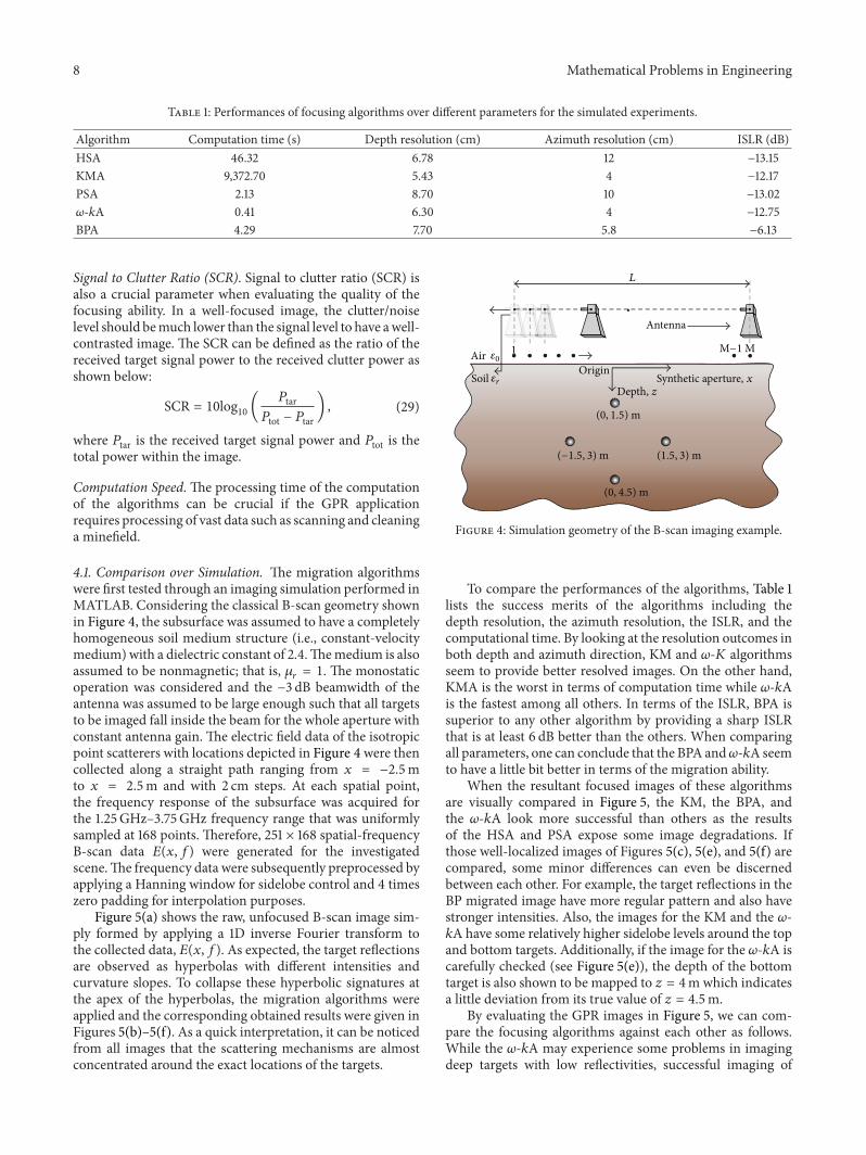
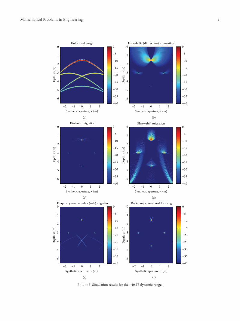
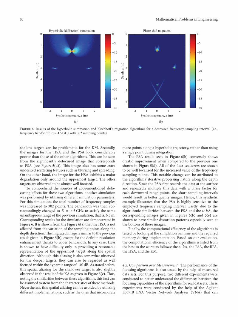
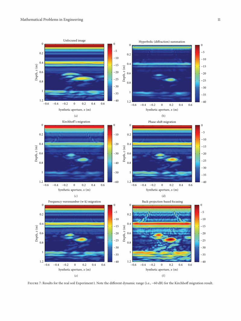
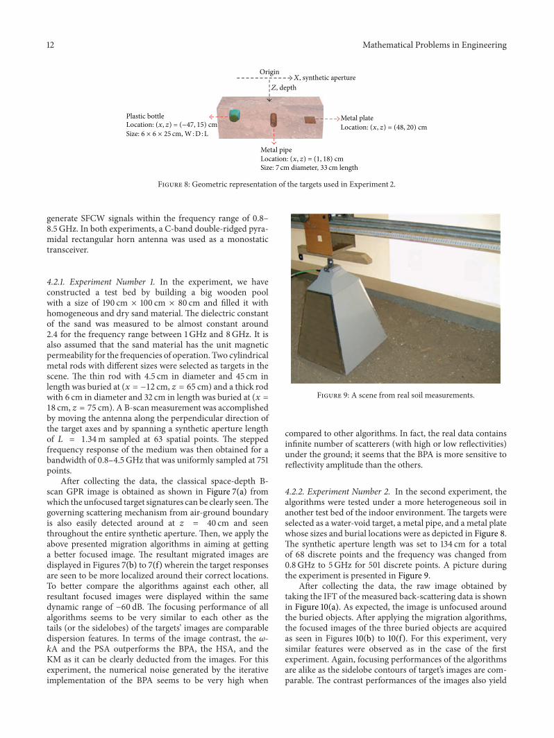
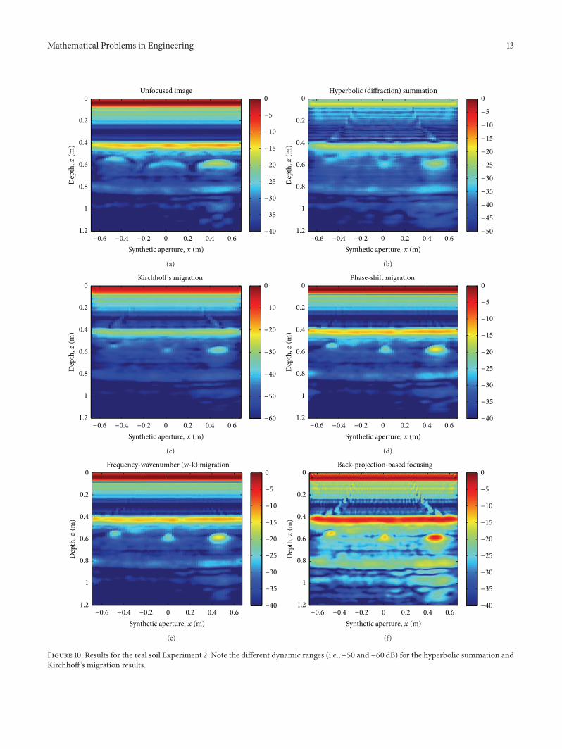
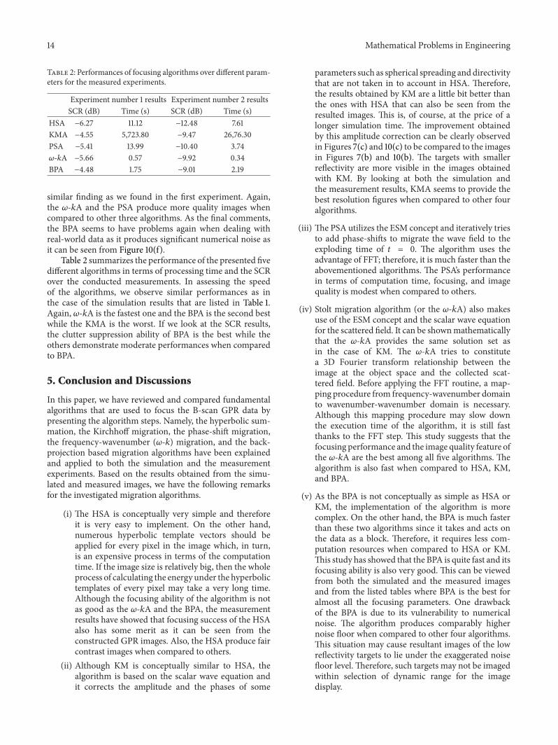the different trip times of the EM wave while the antennais moving along the scanning direction For this reasonthe resolution along the synthetic aperture direction depictsundesired low resolution features owing to the long tails ofthe hyperbola Therefore one of the most applied problemfor the B-scan GPR image is to transform (or to migrate) theunfocused space-time GPR image to a focused one show-ing the objectrsquos true location and size with correspondingEM reflectivity The common name for this task is calledmigration or focusing [5ndash18] In fact migrationmethods wereprimarily developed for processing seismic images [19] andthey were also applied to the GPR thanks to the likenessesbetween the acoustic and the electromagnetic wave equations[7ndash11] Kirchhoff rsquos wave-equation [5] and frequency-wavenumber (120596-119896) based [6 7] migration algorithms are widelyrecognized and employed The wave number domain focus-ing techniques for instance were first formulated for seismicimaging applications [7] and then adapted to the contempo-rary synthetic aperture radar (SAR) imaging practices [12ndash15] These algorithms are also named as seismic migration[12 13] and frequency-wave number (or 120596-119896) migration [16ndash18] by different researchers

In this work we present a brief review of the B-scanGPR migrationfocusing methods that are commonly usedby GPR research community Although we have done somepreliminary studies on the performance comparison of onlytwo GPR focusing algorithms earlier [20] by utilizing verylimited performance parameters in this paper we extendour studies to compare a total of five popular algorithms byassessing different aspects of these algorithms In Section 2we address the problem of migration together with the well-known exploding source concept In fact most migrationalgorithms make use of this concept as we shall explainin this work In Section 3 most popular and functionalmigration methods for the B-scan GPR imaging applicationsare reviewed For this purpose (i) hyperbolic summation(ii) Kirchhoff rsquos migration (iii) phase-shift migration (iv)frequency-wavenumber (or the 120596-119896) migration and (v)back-projection method are presented together with thedetailed algorithm steps In Section 4 the success and theperformance of these algorithms were compared to eachother by testing them over the simulated and the measuredB-scan GPR data Our main objective in this work is topresent a qualitative comparison of these popular and widelyused algorithms such that the reader can benefit from theperformance results over different parameters ranging fromresolution to computation time Section 5 is dedicated todiscussions and the conclusion

2 The Problem of MigrationFocusing

The common goal in a typical GPR image is to display theinformation of the spatial location and the reflectivity of anunderground object As illustrated in Figure 1 a single pointscatterer appears as a hyperbola in the space-time GPR imagefor themonostatic operation Since this is the expected imagepattern for the B-scan operation such information can bethought as sufficient if the main goal of the GPR application

is just to sense a pipe or comparable objects However theinformation about the scatterer including its depth its sizeand its EM reflectivity can be very important in most GPRapplications Therefore the hyperbola or dispersion in thespace-time B-scan GPR image ought to be converted to afocused one that demonstrates the objectrsquos factual locationand size together with its scattering amplitude A focusedor migrated image is gathered after the elimination of thishyperbolic type of diffraction or any other kind of dispersion[5ndash18]

21 Exploding Source Model Most of the migration methodsare based on the concept called exploding source model(ESM) In 1985 Claerbout [21] came with the clever idea ofthinking of the scattered field at the radar receiver as if itis originated from the source at the target location Insteadof assuming a two-way trip convention of the EM wavetherefore it is imagined that a fictitious source ldquoexploderdquo ata reference time of 119905 = 0 around the target location andsend EM wave to the receiver as illustrated in Figure 2 Thereal data collection scheme is shown in Figure 2(a) wherein fact the two-way propagation between the radar and theobject existsWhen theESM is utilized however the collecteddata is assumed to be originally radiated from the source onthe object Therefore one-way propagation is assumed in theESM depicted in Figure 2(b) Since the trip time of the EMwave would be half of the original problem the compensationshould be made for the velocity of the EM wave by justdividing it by two to have V

119898= V2 where V is the speed of

the EM wave within the medium of propagationThe migration using the ESM is essentially carried out by

applying these two actions

(i) the received signal is extrapolated back to explodingsource points

(ii) the migrated image is realized by forming the backextrapolated EM wave at the time of 119905 = 0

3 MigrationFocusing Methods

In this section we will briefly review the basic steps of themostly applied GPR algorithms namely the hyperbolic sum-mation the Kirchhoff migration the phase-shift migrationthe 120596-119896 (Stolt) migration and the back-projection focusingOther migration methods will also be mentioned at the endof this section

31 Hyperbolic (Diffraction) Summation In a typical GPRapplication the radar antenna collects the scattered or back-scattered EM wave from the air-to-ground interface andsubsurface objects together with many cluttering effectsmainly attributed to inhomogeneities within the ground Forthe idealistic case the phase of the scattered signal is directlyproportional to the trip time (or distance) that the EMwave possesses if the propagation medium is homogenousThe monostatic backscattered signal from a single point-likescatterer experiences different round-trip distances while theantenna is moving over the surface for the B-scan operation


Antenna

Sub-surface

1 2 Mminus1 M3

120576r

Air1205760


x

z

R1R2 R3

Space x

Time t

t3 = R3

t2 = R2

Object

(a)

(b)

t1 = R1


120576r

Air 1205760

Object

Two-waypropagation

m = c

Subsurface

(a)

120576r

Antenna


Object

One-waypropagation

m = c2

Subsurface

(b)








R = radic1199112

119900+ (X minus 119909

119900)2

(1)







rms at (119909119894 119911119894) =

radic(

1003816100381610038161003816Es10038161003816

10038161003816

210038161003816100381610038161003816(Es

)lowast10038161003816

100381610038161003816

2

)

119873

=

1

radic119873

119873

sum

119894=1

1003816100381610038161003816Esi1003816100381610038161003816

2

(2)


119894 119911119894) This process is




(

1205972

1205971199092

+

1205972

1205971199112

minus

1

V2119898

1205972

1205971199052

) 120593 (119909 119911 119905) = 0 (3)



119875 (119909 119911 119905) =

1

2120587

int

infin

minusinfin

(

cos 120579

V119898

119877

sdot

120597

120597119905

119875 (119909 119911 119905 minus

119903

V119898

)) 119889119909 (4)


and 119903 = ((119909 minus 119909119898

)2

+ 1199112

)


119898 0)




119898119903) for the 3D








119911119911)





119870 = 119890119895119896119911sdotΔ119911

(5)


119909) as

119870 = exp (119895119896119911

sdot Δ119911)

= exp (119895radic1198962

minus 1198962

119909sdot Δ119911)


119896119909

119896

)

2

sdot Δ119911)

(6)


119898


119870 = exp(119895

119908


V119898

sdot 119896119909

120596

)

2

) (7)




data via Δ119911 = V119898



V119898

sdot 119896119909

120596

)

2

) (8)





119904




119909 119896119911) domain as

1198641199041015840

(120596 119896119909 119896119911) = 119870 sdot 119864

119904(120596 119896119909) (9)

The new dataset 1198641199041015840



119864119904

(119896119909 119896119911 119905) = sum

119908

1198641199041015840

(120596 119896119909 119896119911) (10)



(119909 119911) = IFT 119864119904

(119896119909 119896119911) (11)



(

1205972

1205971199092

+

1205972

1205971199102

+

1205972

1205971199112

minus

1

V2119898

1205972

1205971199052

) 120593 (119909 119910 119911 119905) = 0 (12)


1198962

119909+ 1198962

119910+ 1198962

119911= 1198962

=

1205962

V2119898

(13)


119909 119896119910

120596) as

120593 (119909 119910 119911 119905) = (

1

2120587

)

32

∭

infin

minusinfin

119864 (119896119909 119896119910

120596)


119889119896119909119889119896119910

119889120596

(14)


120593 (119909 119910 0 119905) ≜ 119890 (119909 119910 119905)

= (

1

2120587

)

32

∭

infin

minusinfin

119864 (119896119909 119896119910

120596)


119889119896119909119889119896119910

119889120596

(15)



119864 (119896119909 119896119910

120596) = (

1

2120587

)

32

∭

infin

minusinfin

119890 (119909 119910 119905)

times 119890119895(119896119909119909+119896119910119910minus120596119905)

119889119909 119889119910 119889119905

(16)


119864 (119896119909 119896119910

120596) = 119890119895119896119911119911

119864 (119896119909 119896119910

120596 119911 = 0) (17)


119890 (119909 119910 119911 0) = (

1

2120587

)

32

∭

infin

minusinfin

119864 (119896119909 119896119910

120596)

times 119890minus119895(119896119909119909+119896119910119910+119896119911119911)

119889119896119909119889119896119910

119889120596

(18)


119909 119896119910






120596 = V119898

(1198962

119909+ 1198962

119910+ 1198962

119911)

12 (19a)

119889120596 =

V2119898

119896119911

120596

119889119896119911 (19b)


119890 (119909 119910 119911) = (

1

2120587

)

32

∭

infin

minusinfin

V2119898

119896119911

120596

119864119898

(119896119909 119896119910

119896119911)

times 119890minus119895(119896119909119909+119896119910119910+119896119911119911)

119889119896119909119889119896119910

119889119896119911

(20)

Here 119864119898

(119896119909 119896119910


data 119864(119896119909 119896119910




Soil

h

120576r

Air 1205760

Imaging scene

Scenecenter

(x0 z0)

rm

um

120579m

x

x

z

z

Range(depth)

(xm zm)


(((xxx0 zzzz0)))

rmmrr

uumm

120579120579120579mm

xxxx

zz






119890 (119909 119911) = (

1

2120587

) ∬

infin

minusinfin

V2119898

119896119911

120596

119864119898

(119896119909 119896119911)

times 119890minus119895(119896119909119909+119896119911119911)

119889119896119909119889119896119911

(21)




119903and


119898 119911119898


119898is


119878120579119898

[119896119903] = ∬

infin

minusinfin

119890 (119909 119911) exp (minus119895119896119903119903119898

) 119889119909 119889119911 (22)


agation as 119896119903




119911119898



119904120579119898

(119903) equiv IFT 119878120579119898

(119896119903)

= ∬

infin

minusinfin

119890 (119909 119911) 120575 (119903119898

minus 119903) 119889119909 119889119911

(23)




119890 (119909 119911) = ∬

infin

minusinfin

119864 (119896119909 119896119911) exp [119895 (119896

119909119909 + 119896119911119911)] 119889119896

119909119889119896119911 (24)



) asfollows

119890 (119909 119911) = int

120587

minus120587

int

infin

0

119864 (119896119903 120579119898

) exp (119895119896119903119903119898

) 119896119903119889119896119903119889120579119898

(25)



120579(119896119903)






119890 (119909 119911) = int

120587

minus120587

[int

infin

0

119878120579119898

(119896119903) exp (119895119896

119903119903119898

) 119896119903119889119896119903] 119889120579119898

(26)


120579119898

(119896119903) = 119878

120579119898

(119896119903)119896119903calculated at

119903119898 Defining 119902

120579119898


120588 (119909 119911) = int

120587

minus120587

119902120579119898

(119903119898

) 119889120579119898

(27)




(119896119903)

with 119896119903



(119903)



120579119898

(119903119898

)




119898






ISLR = 10log10

(

intminus3 dB 119868119889119909

1015840

1198891199101015840

int

+infin

minusinfin

11986811988911990910158401198891199101015840


10158401198891199101015840

) (28)


1015840



+infin

minusinfin

1198681198891199091015840






SCR = 10log10

(


) (29)







Antenna

Soil

1 Mminus1 M

L

120576r

Air 1205760

(0 15) m


Origin

(0 45) m

(minus15 3) m (15 3) m






Unfocused image0

1

2

3

4

5

6


Dep

thz

(m)


minus35

minus30

minus25

minus20

minus15

minus10

minus5

0

(a)


1

2

3

4

5

6


Dep

thz

(m)


minus35

minus30

minus25

minus20

minus15

minus10

minus5

0

(b)


1

2

3

4

5

6


Dep

thz

(m)


minus35

minus30

minus25

minus20

minus15

minus10

minus5

0

(c)


1

2

3

4

5

6


Dep

thz

(m)


minus35

minus30

minus25

minus20

minus15

minus10

minus5

0

(d)

0

1

2

3

4

5

6


Dep

thz

(m)


minus35

minus30

minus25

minus20

minus15

minus10

minus5


(e)


1

2

3

4

5

6


Dep

thz

(m)


minus35

minus30

minus25

minus20

minus15

minus10

minus5

0

(f)




1

2

3

4

5

6


Dep

thz

(m)


minus35

minus30

minus25

minus20

minus15

minus10

minus5

0

(a)


1

2

3

4

5

6


Dep

thz

(m)


minus35

minus30

minus25

minus20

minus15

minus10

minus5

0

(b)









Unfocused image0

02

04

06

08

1

12


Dep

thz

(m)

minus40

minus35

minus30

minus25

minus20

minus15

minus10

minus5

0


(a)


02

04

06

08

1

12


Dep

thz

(m)

minus40

minus35

minus30

minus25

minus20

minus15

minus10

minus5

0


(b)


02

04

06

08

1

12


Dep

thz

(m)

minus40

minus50

minus60

minus30

minus20

minus10

0


(c)


02

04

06

08

1

12


Dep

thz

(m)

minus40

minus35

minus30

minus25

minus20

minus15

minus10

minus5

0


(d)

0

02

04

06

08

1

12


Dep

thz

(m)

minus40

minus35

minus30

minus25

minus20

minus15

minus10

minus5

0



(e)


02

04

06

08

1

12


Dep

thz

(m)

minus40

minus35

minus30

minus25

minus20

minus15

minus10

minus5

0


(f)




Origin














Unfocused image0

02

04

06

08

1


minus40

minus35

minus30

minus25

minus20

minus15

minus10

minus5

0


Dep

thz

(m)

(a)


02

04

06

08

1


minus40

minus45

minus50

minus35

minus30

minus25

minus20

minus15

minus10

minus5

0


Dep

thz

(m)

(b)


02

04

06

08

1


minus40

minus50

minus60

minus30

minus20

minus10

0


Dep

thz

(m)

(c)


02

04

06

08

1


minus40

minus35

minus30

minus25

minus20

minus15

minus10

minus5

0


Dep

thz

(m)

(d)

0

02

04

06

08

1


minus40

minus35

minus30

minus25

minus20

minus15

minus10

minus5

0


Dep

thz

(m)


(e)


02

04

06

08

1


minus40

minus35

minus30

minus25

minus20

minus15

minus10

minus5

0


Dep

thz

(m)

(f)



















Acknowledgment


References













































Volume 2014




Journal of











Journal of


Function Spaces






Algebra










Antenna

Sub-surface

1 2 Mminus1 M3

120576r

Air1205760


x

z

R1R2 R3

Space x

Time t

t3 = R3

t2 = R2

Object

(a)

(b)

t1 = R1


120576r

Air 1205760

Object

Two-waypropagation

m = c

Subsurface

(a)

120576r

Antenna


Object

One-waypropagation

m = c2

Subsurface

(b)








R = radic1199112

119900+ (X minus 119909

119900)2

(1)







rms at (119909119894 119911119894) =

radic(

1003816100381610038161003816Es10038161003816

10038161003816

210038161003816100381610038161003816(Es

)lowast10038161003816

100381610038161003816

2

)

119873

=

1

radic119873

119873

sum

119894=1

1003816100381610038161003816Esi1003816100381610038161003816

2

(2)


119894 119911119894) This process is




(

1205972

1205971199092

+

1205972

1205971199112

minus

1

V2119898

1205972

1205971199052

) 120593 (119909 119911 119905) = 0 (3)



119875 (119909 119911 119905) =

1

2120587

int

infin

minusinfin

(

cos 120579

V119898

119877

sdot

120597

120597119905

119875 (119909 119911 119905 minus

119903

V119898

)) 119889119909 (4)


and 119903 = ((119909 minus 119909119898

)2

+ 1199112

)


119898 0)




119898119903) for the 3D








119911119911)





119870 = 119890119895119896119911sdotΔ119911

(5)


119909) as

119870 = exp (119895119896119911

sdot Δ119911)

= exp (119895radic1198962

minus 1198962

119909sdot Δ119911)


119896119909

119896

)

2

sdot Δ119911)

(6)


119898


119870 = exp(119895

119908


V119898

sdot 119896119909

120596

)

2

) (7)




data via Δ119911 = V119898



V119898

sdot 119896119909

120596

)

2

) (8)





119904




119909 119896119911) domain as

1198641199041015840

(120596 119896119909 119896119911) = 119870 sdot 119864

119904(120596 119896119909) (9)

The new dataset 1198641199041015840



119864119904

(119896119909 119896119911 119905) = sum

119908

1198641199041015840

(120596 119896119909 119896119911) (10)



(119909 119911) = IFT 119864119904

(119896119909 119896119911) (11)



(

1205972

1205971199092

+

1205972

1205971199102

+

1205972

1205971199112

minus

1

V2119898

1205972

1205971199052

) 120593 (119909 119910 119911 119905) = 0 (12)


1198962

119909+ 1198962

119910+ 1198962

119911= 1198962

=

1205962

V2119898

(13)


119909 119896119910

120596) as

120593 (119909 119910 119911 119905) = (

1

2120587

)

32

∭

infin

minusinfin

119864 (119896119909 119896119910

120596)


119889119896119909119889119896119910

119889120596

(14)


120593 (119909 119910 0 119905) ≜ 119890 (119909 119910 119905)

= (

1

2120587

)

32

∭

infin

minusinfin

119864 (119896119909 119896119910

120596)


119889119896119909119889119896119910

119889120596

(15)



119864 (119896119909 119896119910

120596) = (

1

2120587

)

32

∭

infin

minusinfin

119890 (119909 119910 119905)

times 119890119895(119896119909119909+119896119910119910minus120596119905)

119889119909 119889119910 119889119905

(16)


119864 (119896119909 119896119910

120596) = 119890119895119896119911119911

119864 (119896119909 119896119910

120596 119911 = 0) (17)


119890 (119909 119910 119911 0) = (

1

2120587

)

32

∭

infin

minusinfin

119864 (119896119909 119896119910

120596)

times 119890minus119895(119896119909119909+119896119910119910+119896119911119911)

119889119896119909119889119896119910

119889120596

(18)


119909 119896119910






120596 = V119898

(1198962

119909+ 1198962

119910+ 1198962

119911)

12 (19a)

119889120596 =

V2119898

119896119911

120596

119889119896119911 (19b)


119890 (119909 119910 119911) = (

1

2120587

)

32

∭

infin

minusinfin

V2119898

119896119911

120596

119864119898

(119896119909 119896119910

119896119911)

times 119890minus119895(119896119909119909+119896119910119910+119896119911119911)

119889119896119909119889119896119910

119889119896119911

(20)

Here 119864119898

(119896119909 119896119910


data 119864(119896119909 119896119910




Soil

h

120576r

Air 1205760

Imaging scene

Scenecenter

(x0 z0)

rm

um

120579m

x

x

z

z

Range(depth)

(xm zm)


(((xxx0 zzzz0)))

rmmrr

uumm

120579120579120579mm

xxxx

zz






119890 (119909 119911) = (

1

2120587

) ∬

infin

minusinfin

V2119898

119896119911

120596

119864119898

(119896119909 119896119911)

times 119890minus119895(119896119909119909+119896119911119911)

119889119896119909119889119896119911

(21)




119903and


119898 119911119898


119898is


119878120579119898

[119896119903] = ∬

infin

minusinfin

119890 (119909 119911) exp (minus119895119896119903119903119898

) 119889119909 119889119911 (22)


agation as 119896119903




119911119898



119904120579119898

(119903) equiv IFT 119878120579119898

(119896119903)

= ∬

infin

minusinfin

119890 (119909 119911) 120575 (119903119898

minus 119903) 119889119909 119889119911

(23)




119890 (119909 119911) = ∬

infin

minusinfin

119864 (119896119909 119896119911) exp [119895 (119896

119909119909 + 119896119911119911)] 119889119896

119909119889119896119911 (24)



) asfollows

119890 (119909 119911) = int

120587

minus120587

int

infin

0

119864 (119896119903 120579119898

) exp (119895119896119903119903119898

) 119896119903119889119896119903119889120579119898

(25)



120579(119896119903)






119890 (119909 119911) = int

120587

minus120587

[int

infin

0

119878120579119898

(119896119903) exp (119895119896

119903119903119898

) 119896119903119889119896119903] 119889120579119898

(26)


120579119898

(119896119903) = 119878

120579119898

(119896119903)119896119903calculated at

119903119898 Defining 119902

120579119898


120588 (119909 119911) = int

120587

minus120587

119902120579119898

(119903119898

) 119889120579119898

(27)




(119896119903)

with 119896119903



(119903)



120579119898

(119903119898

)




119898






ISLR = 10log10

(

intminus3 dB 119868119889119909

1015840

1198891199101015840

int

+infin

minusinfin

11986811988911990910158401198891199101015840


10158401198891199101015840

) (28)


1015840



+infin

minusinfin

1198681198891199091015840






SCR = 10log10

(


) (29)







Antenna

Soil

1 Mminus1 M

L

120576r

Air 1205760

(0 15) m


Origin

(0 45) m

(minus15 3) m (15 3) m






Unfocused image0

1

2

3

4

5

6


Dep

thz

(m)


minus35

minus30

minus25

minus20

minus15

minus10

minus5

0

(a)


1

2

3

4

5

6


Dep

thz

(m)


minus35

minus30

minus25

minus20

minus15

minus10

minus5

0

(b)


1

2

3

4

5

6


Dep

thz

(m)


minus35

minus30

minus25

minus20

minus15

minus10

minus5

0

(c)


1

2

3

4

5

6


Dep

thz

(m)


minus35

minus30

minus25

minus20

minus15

minus10

minus5

0

(d)

0

1

2

3

4

5

6


Dep

thz

(m)


minus35

minus30

minus25

minus20

minus15

minus10

minus5


(e)


1

2

3

4

5

6


Dep

thz

(m)


minus35

minus30

minus25

minus20

minus15

minus10

minus5

0

(f)




1

2

3

4

5

6


Dep

thz

(m)


minus35

minus30

minus25

minus20

minus15

minus10

minus5

0

(a)


1

2

3

4

5

6


Dep

thz

(m)


minus35

minus30

minus25

minus20

minus15

minus10

minus5

0

(b)









Unfocused image0

02

04

06

08

1

12


Dep

thz

(m)

minus40

minus35

minus30

minus25

minus20

minus15

minus10

minus5

0


(a)


02

04

06

08

1

12


Dep

thz

(m)

minus40

minus35

minus30

minus25

minus20

minus15

minus10

minus5

0


(b)


02

04

06

08

1

12


Dep

thz

(m)

minus40

minus50

minus60

minus30

minus20

minus10

0


(c)


02

04

06

08

1

12


Dep

thz

(m)

minus40

minus35

minus30

minus25

minus20

minus15

minus10

minus5

0


(d)

0

02

04

06

08

1

12


Dep

thz

(m)

minus40

minus35

minus30

minus25

minus20

minus15

minus10

minus5

0



(e)


02

04

06

08

1

12


Dep

thz

(m)

minus40

minus35

minus30

minus25

minus20

minus15

minus10

minus5

0


(f)




Origin














Unfocused image0

02

04

06

08

1


minus40

minus35

minus30

minus25

minus20

minus15

minus10

minus5

0


Dep

thz

(m)

(a)


02

04

06

08

1


minus40

minus45

minus50

minus35

minus30

minus25

minus20

minus15

minus10

minus5

0


Dep

thz

(m)

(b)


02

04

06

08

1


minus40

minus50

minus60

minus30

minus20

minus10

0


Dep

thz

(m)

(c)


02

04

06

08

1


minus40

minus35

minus30

minus25

minus20

minus15

minus10

minus5

0


Dep

thz

(m)

(d)

0

02

04

06

08

1


minus40

minus35

minus30

minus25

minus20

minus15

minus10

minus5

0


Dep

thz

(m)


(e)


02

04

06

08

1


minus40

minus35

minus30

minus25

minus20

minus15

minus10

minus5

0


Dep

thz

(m)

(f)



















Acknowledgment


References













































Volume 2014




Journal of











Journal of


Function Spaces






Algebra











R = radic1199112

119900+ (X minus 119909

119900)2

(1)







rms at (119909119894 119911119894) =

radic(

1003816100381610038161003816Es10038161003816

10038161003816

210038161003816100381610038161003816(Es

)lowast10038161003816

100381610038161003816

2

)

119873

=

1

radic119873

119873

sum

119894=1

1003816100381610038161003816Esi1003816100381610038161003816

2

(2)


119894 119911119894) This process is




(

1205972

1205971199092

+

1205972

1205971199112

minus

1

V2119898

1205972

1205971199052

) 120593 (119909 119911 119905) = 0 (3)



119875 (119909 119911 119905) =

1

2120587

int

infin

minusinfin

(

cos 120579

V119898

119877

sdot

120597

120597119905

119875 (119909 119911 119905 minus

119903

V119898

)) 119889119909 (4)


and 119903 = ((119909 minus 119909119898

)2

+ 1199112

)


119898 0)




119898119903) for the 3D








119911119911)





119870 = 119890119895119896119911sdotΔ119911

(5)


119909) as

119870 = exp (119895119896119911

sdot Δ119911)

= exp (119895radic1198962

minus 1198962

119909sdot Δ119911)


119896119909

119896

)

2

sdot Δ119911)

(6)


119898


119870 = exp(119895

119908


V119898

sdot 119896119909

120596

)

2

) (7)




data via Δ119911 = V119898



V119898

sdot 119896119909

120596

)

2

) (8)





119904




119909 119896119911) domain as

1198641199041015840

(120596 119896119909 119896119911) = 119870 sdot 119864

119904(120596 119896119909) (9)

The new dataset 1198641199041015840



119864119904

(119896119909 119896119911 119905) = sum

119908

1198641199041015840

(120596 119896119909 119896119911) (10)



(119909 119911) = IFT 119864119904

(119896119909 119896119911) (11)



(

1205972

1205971199092

+

1205972

1205971199102

+

1205972

1205971199112

minus

1

V2119898

1205972

1205971199052

) 120593 (119909 119910 119911 119905) = 0 (12)


1198962

119909+ 1198962

119910+ 1198962

119911= 1198962

=

1205962

V2119898

(13)


119909 119896119910

120596) as

120593 (119909 119910 119911 119905) = (

1

2120587

)

32

∭

infin

minusinfin

119864 (119896119909 119896119910

120596)


119889119896119909119889119896119910

119889120596

(14)


120593 (119909 119910 0 119905) ≜ 119890 (119909 119910 119905)

= (

1

2120587

)

32

∭

infin

minusinfin

119864 (119896119909 119896119910

120596)


119889119896119909119889119896119910

119889120596

(15)



119864 (119896119909 119896119910

120596) = (

1

2120587

)

32

∭

infin

minusinfin

119890 (119909 119910 119905)

times 119890119895(119896119909119909+119896119910119910minus120596119905)

119889119909 119889119910 119889119905

(16)


119864 (119896119909 119896119910

120596) = 119890119895119896119911119911

119864 (119896119909 119896119910

120596 119911 = 0) (17)


119890 (119909 119910 119911 0) = (

1

2120587

)

32

∭

infin

minusinfin

119864 (119896119909 119896119910

120596)

times 119890minus119895(119896119909119909+119896119910119910+119896119911119911)

119889119896119909119889119896119910

119889120596

(18)


119909 119896119910






120596 = V119898

(1198962

119909+ 1198962

119910+ 1198962

119911)

12 (19a)

119889120596 =

V2119898

119896119911

120596

119889119896119911 (19b)


119890 (119909 119910 119911) = (

1

2120587

)

32

∭

infin

minusinfin

V2119898

119896119911

120596

119864119898

(119896119909 119896119910

119896119911)

times 119890minus119895(119896119909119909+119896119910119910+119896119911119911)

119889119896119909119889119896119910

119889119896119911

(20)

Here 119864119898

(119896119909 119896119910


data 119864(119896119909 119896119910




Soil

h

120576r

Air 1205760

Imaging scene

Scenecenter

(x0 z0)

rm

um

120579m

x

x

z

z

Range(depth)

(xm zm)


(((xxx0 zzzz0)))

rmmrr

uumm

120579120579120579mm

xxxx

zz






119890 (119909 119911) = (

1

2120587

) ∬

infin

minusinfin

V2119898

119896119911

120596

119864119898

(119896119909 119896119911)

times 119890minus119895(119896119909119909+119896119911119911)

119889119896119909119889119896119911

(21)




119903and


119898 119911119898


119898is


119878120579119898

[119896119903] = ∬

infin

minusinfin

119890 (119909 119911) exp (minus119895119896119903119903119898

) 119889119909 119889119911 (22)


agation as 119896119903




119911119898



119904120579119898

(119903) equiv IFT 119878120579119898

(119896119903)

= ∬

infin

minusinfin

119890 (119909 119911) 120575 (119903119898

minus 119903) 119889119909 119889119911

(23)




119890 (119909 119911) = ∬

infin

minusinfin

119864 (119896119909 119896119911) exp [119895 (119896

119909119909 + 119896119911119911)] 119889119896

119909119889119896119911 (24)



) asfollows

119890 (119909 119911) = int

120587

minus120587

int

infin

0

119864 (119896119903 120579119898

) exp (119895119896119903119903119898

) 119896119903119889119896119903119889120579119898

(25)



120579(119896119903)






119890 (119909 119911) = int

120587

minus120587

[int

infin

0

119878120579119898

(119896119903) exp (119895119896

119903119903119898

) 119896119903119889119896119903] 119889120579119898

(26)


120579119898

(119896119903) = 119878

120579119898

(119896119903)119896119903calculated at

119903119898 Defining 119902

120579119898


120588 (119909 119911) = int

120587

minus120587

119902120579119898

(119903119898

) 119889120579119898

(27)




(119896119903)

with 119896119903



(119903)



120579119898

(119903119898

)




119898






ISLR = 10log10

(

intminus3 dB 119868119889119909

1015840

1198891199101015840

int

+infin

minusinfin

11986811988911990910158401198891199101015840


10158401198891199101015840

) (28)


1015840



+infin

minusinfin

1198681198891199091015840






SCR = 10log10

(


) (29)







Antenna

Soil

1 Mminus1 M

L

120576r

Air 1205760

(0 15) m


Origin

(0 45) m

(minus15 3) m (15 3) m






Unfocused image0

1

2

3

4

5

6


Dep

thz

(m)


minus35

minus30

minus25

minus20

minus15

minus10

minus5

0

(a)


1

2

3

4

5

6


Dep

thz

(m)


minus35

minus30

minus25

minus20

minus15

minus10

minus5

0

(b)


1

2

3

4

5

6


Dep

thz

(m)


minus35

minus30

minus25

minus20

minus15

minus10

minus5

0

(c)


1

2

3

4

5

6


Dep

thz

(m)


minus35

minus30

minus25

minus20

minus15

minus10

minus5

0

(d)

0

1

2

3

4

5

6


Dep

thz

(m)


minus35

minus30

minus25

minus20

minus15

minus10

minus5


(e)


1

2

3

4

5

6


Dep

thz

(m)


minus35

minus30

minus25

minus20

minus15

minus10

minus5

0

(f)




1

2

3

4

5

6


Dep

thz

(m)


minus35

minus30

minus25

minus20

minus15

minus10

minus5

0

(a)


1

2

3

4

5

6


Dep

thz

(m)


minus35

minus30

minus25

minus20

minus15

minus10

minus5

0

(b)









Unfocused image0

02

04

06

08

1

12


Dep

thz

(m)

minus40

minus35

minus30

minus25

minus20

minus15

minus10

minus5

0


(a)


02

04

06

08

1

12


Dep

thz

(m)

minus40

minus35

minus30

minus25

minus20

minus15

minus10

minus5

0


(b)


02

04

06

08

1

12


Dep

thz

(m)

minus40

minus50

minus60

minus30

minus20

minus10

0


(c)


02

04

06

08

1

12


Dep

thz

(m)

minus40

minus35

minus30

minus25

minus20

minus15

minus10

minus5

0


(d)

0

02

04

06

08

1

12


Dep

thz

(m)

minus40

minus35

minus30

minus25

minus20

minus15

minus10

minus5

0



(e)


02

04

06

08

1

12


Dep

thz

(m)

minus40

minus35

minus30

minus25

minus20

minus15

minus10

minus5

0


(f)




Origin














Unfocused image0

02

04

06

08

1


minus40

minus35

minus30

minus25

minus20

minus15

minus10

minus5

0


Dep

thz

(m)

(a)


02

04

06

08

1


minus40

minus45

minus50

minus35

minus30

minus25

minus20

minus15

minus10

minus5

0


Dep

thz

(m)

(b)


02

04

06

08

1


minus40

minus50

minus60

minus30

minus20

minus10

0


Dep

thz

(m)

(c)


02

04

06

08

1


minus40

minus35

minus30

minus25

minus20

minus15

minus10

minus5

0


Dep

thz

(m)

(d)

0

02

04

06

08

1


minus40

minus35

minus30

minus25

minus20

minus15

minus10

minus5

0


Dep

thz

(m)


(e)


02

04

06

08

1


minus40

minus35

minus30

minus25

minus20

minus15

minus10

minus5

0


Dep

thz

(m)

(f)



















Acknowledgment


References













































Volume 2014




Journal of











Journal of


Function Spaces






Algebra










data via Δ119911 = V119898



V119898

sdot 119896119909

120596

)

2

) (8)





119904




119909 119896119911) domain as

1198641199041015840

(120596 119896119909 119896119911) = 119870 sdot 119864

119904(120596 119896119909) (9)

The new dataset 1198641199041015840



119864119904

(119896119909 119896119911 119905) = sum

119908

1198641199041015840

(120596 119896119909 119896119911) (10)



(119909 119911) = IFT 119864119904

(119896119909 119896119911) (11)



(

1205972

1205971199092

+

1205972

1205971199102

+

1205972

1205971199112

minus

1

V2119898

1205972

1205971199052

) 120593 (119909 119910 119911 119905) = 0 (12)


1198962

119909+ 1198962

119910+ 1198962

119911= 1198962

=

1205962

V2119898

(13)


119909 119896119910

120596) as

120593 (119909 119910 119911 119905) = (

1

2120587

)

32

∭

infin

minusinfin

119864 (119896119909 119896119910

120596)


119889119896119909119889119896119910

119889120596

(14)


120593 (119909 119910 0 119905) ≜ 119890 (119909 119910 119905)

= (

1

2120587

)

32

∭

infin

minusinfin

119864 (119896119909 119896119910

120596)


119889119896119909119889119896119910

119889120596

(15)



119864 (119896119909 119896119910

120596) = (

1

2120587

)

32

∭

infin

minusinfin

119890 (119909 119910 119905)

times 119890119895(119896119909119909+119896119910119910minus120596119905)

119889119909 119889119910 119889119905

(16)


119864 (119896119909 119896119910

120596) = 119890119895119896119911119911

119864 (119896119909 119896119910

120596 119911 = 0) (17)


119890 (119909 119910 119911 0) = (

1

2120587

)

32

∭

infin

minusinfin

119864 (119896119909 119896119910

120596)

times 119890minus119895(119896119909119909+119896119910119910+119896119911119911)

119889119896119909119889119896119910

119889120596

(18)


119909 119896119910






120596 = V119898

(1198962

119909+ 1198962

119910+ 1198962

119911)

12 (19a)

119889120596 =

V2119898

119896119911

120596

119889119896119911 (19b)


119890 (119909 119910 119911) = (

1

2120587

)

32

∭

infin

minusinfin

V2119898

119896119911

120596

119864119898

(119896119909 119896119910

119896119911)

times 119890minus119895(119896119909119909+119896119910119910+119896119911119911)

119889119896119909119889119896119910

119889119896119911

(20)

Here 119864119898

(119896119909 119896119910


data 119864(119896119909 119896119910




Soil

h

120576r

Air 1205760

Imaging scene

Scenecenter

(x0 z0)

rm

um

120579m

x

x

z

z

Range(depth)

(xm zm)


(((xxx0 zzzz0)))

rmmrr

uumm

120579120579120579mm

xxxx

zz






119890 (119909 119911) = (

1

2120587

) ∬

infin

minusinfin

V2119898

119896119911

120596

119864119898

(119896119909 119896119911)

times 119890minus119895(119896119909119909+119896119911119911)

119889119896119909119889119896119911

(21)




119903and


119898 119911119898


119898is


119878120579119898

[119896119903] = ∬

infin

minusinfin

119890 (119909 119911) exp (minus119895119896119903119903119898

) 119889119909 119889119911 (22)


agation as 119896119903




119911119898



119904120579119898

(119903) equiv IFT 119878120579119898

(119896119903)

= ∬

infin

minusinfin

119890 (119909 119911) 120575 (119903119898

minus 119903) 119889119909 119889119911

(23)




119890 (119909 119911) = ∬

infin

minusinfin

119864 (119896119909 119896119911) exp [119895 (119896

119909119909 + 119896119911119911)] 119889119896

119909119889119896119911 (24)



) asfollows

119890 (119909 119911) = int

120587

minus120587

int

infin

0

119864 (119896119903 120579119898

) exp (119895119896119903119903119898

) 119896119903119889119896119903119889120579119898

(25)



120579(119896119903)






119890 (119909 119911) = int

120587

minus120587

[int

infin

0

119878120579119898

(119896119903) exp (119895119896

119903119903119898

) 119896119903119889119896119903] 119889120579119898

(26)


120579119898

(119896119903) = 119878

120579119898

(119896119903)119896119903calculated at

119903119898 Defining 119902

120579119898


120588 (119909 119911) = int

120587

minus120587

119902120579119898

(119903119898

) 119889120579119898

(27)




(119896119903)

with 119896119903



(119903)



120579119898

(119903119898

)




119898






ISLR = 10log10

(

intminus3 dB 119868119889119909

1015840

1198891199101015840

int

+infin

minusinfin

11986811988911990910158401198891199101015840


10158401198891199101015840

) (28)


1015840



+infin

minusinfin

1198681198891199091015840






SCR = 10log10

(


) (29)







Antenna

Soil

1 Mminus1 M

L

120576r

Air 1205760

(0 15) m


Origin

(0 45) m

(minus15 3) m (15 3) m






Unfocused image0

1

2

3

4

5

6


Dep

thz

(m)


minus35

minus30

minus25

minus20

minus15

minus10

minus5

0

(a)


1

2

3

4

5

6


Dep

thz

(m)


minus35

minus30

minus25

minus20

minus15

minus10

minus5

0

(b)


1

2

3

4

5

6


Dep

thz

(m)


minus35

minus30

minus25

minus20

minus15

minus10

minus5

0

(c)


1

2

3

4

5

6


Dep

thz

(m)


minus35

minus30

minus25

minus20

minus15

minus10

minus5

0

(d)

0

1

2

3

4

5

6


Dep

thz

(m)


minus35

minus30

minus25

minus20

minus15

minus10

minus5


(e)


1

2

3

4

5

6


Dep

thz

(m)


minus35

minus30

minus25

minus20

minus15

minus10

minus5

0

(f)




1

2

3

4

5

6


Dep

thz

(m)


minus35

minus30

minus25

minus20

minus15

minus10

minus5

0

(a)


1

2

3

4

5

6


Dep

thz

(m)


minus35

minus30

minus25

minus20

minus15

minus10

minus5

0

(b)









Unfocused image0

02

04

06

08

1

12


Dep

thz

(m)

minus40

minus35

minus30

minus25

minus20

minus15

minus10

minus5

0


(a)


02

04

06

08

1

12


Dep

thz

(m)

minus40

minus35

minus30

minus25

minus20

minus15

minus10

minus5

0


(b)


02

04

06

08

1

12


Dep

thz

(m)

minus40

minus50

minus60

minus30

minus20

minus10

0


(c)


02

04

06

08

1

12


Dep

thz

(m)

minus40

minus35

minus30

minus25

minus20

minus15

minus10

minus5

0


(d)

0

02

04

06

08

1

12


Dep

thz

(m)

minus40

minus35

minus30

minus25

minus20

minus15

minus10

minus5

0



(e)


02

04

06

08

1

12


Dep

thz

(m)

minus40

minus35

minus30

minus25

minus20

minus15

minus10

minus5

0


(f)




Origin














Unfocused image0

02

04

06

08

1


minus40

minus35

minus30

minus25

minus20

minus15

minus10

minus5

0


Dep

thz

(m)

(a)


02

04

06

08

1


minus40

minus45

minus50

minus35

minus30

minus25

minus20

minus15

minus10

minus5

0


Dep

thz

(m)

(b)


02

04

06

08

1


minus40

minus50

minus60

minus30

minus20

minus10

0


Dep

thz

(m)

(c)


02

04

06

08

1


minus40

minus35

minus30

minus25

minus20

minus15

minus10

minus5

0


Dep

thz

(m)

(d)

0

02

04

06

08

1


minus40

minus35

minus30

minus25

minus20

minus15

minus10

minus5

0


Dep

thz

(m)


(e)


02

04

06

08

1


minus40

minus35

minus30

minus25

minus20

minus15

minus10

minus5

0


Dep

thz

(m)

(f)



















Acknowledgment


References













































Volume 2014




Journal of











Journal of


Function Spaces






Algebra











Soil

h

120576r

Air 1205760

Imaging scene

Scenecenter

(x0 z0)

rm

um

120579m

x

x

z

z

Range(depth)

(xm zm)


(((xxx0 zzzz0)))

rmmrr

uumm

120579120579120579mm

xxxx

zz






119890 (119909 119911) = (

1

2120587

) ∬

infin

minusinfin

V2119898

119896119911

120596

119864119898

(119896119909 119896119911)

times 119890minus119895(119896119909119909+119896119911119911)

119889119896119909119889119896119911

(21)




119903and


119898 119911119898


119898is


119878120579119898

[119896119903] = ∬

infin

minusinfin

119890 (119909 119911) exp (minus119895119896119903119903119898

) 119889119909 119889119911 (22)


agation as 119896119903




119911119898



119904120579119898

(119903) equiv IFT 119878120579119898

(119896119903)

= ∬

infin

minusinfin

119890 (119909 119911) 120575 (119903119898

minus 119903) 119889119909 119889119911

(23)




119890 (119909 119911) = ∬

infin

minusinfin

119864 (119896119909 119896119911) exp [119895 (119896

119909119909 + 119896119911119911)] 119889119896

119909119889119896119911 (24)



) asfollows

119890 (119909 119911) = int

120587

minus120587

int

infin

0

119864 (119896119903 120579119898

) exp (119895119896119903119903119898

) 119896119903119889119896119903119889120579119898

(25)



120579(119896119903)






119890 (119909 119911) = int

120587

minus120587

[int

infin

0

119878120579119898

(119896119903) exp (119895119896

119903119903119898

) 119896119903119889119896119903] 119889120579119898

(26)


120579119898

(119896119903) = 119878

120579119898

(119896119903)119896119903calculated at

119903119898 Defining 119902

120579119898


120588 (119909 119911) = int

120587

minus120587

119902120579119898

(119903119898

) 119889120579119898

(27)




(119896119903)

with 119896119903



(119903)



120579119898

(119903119898

)




119898






ISLR = 10log10

(

intminus3 dB 119868119889119909

1015840

1198891199101015840

int

+infin

minusinfin

11986811988911990910158401198891199101015840


10158401198891199101015840

) (28)


1015840



+infin

minusinfin

1198681198891199091015840






SCR = 10log10

(


) (29)







Antenna

Soil

1 Mminus1 M

L

120576r

Air 1205760

(0 15) m


Origin

(0 45) m

(minus15 3) m (15 3) m






Unfocused image0

1

2

3

4

5

6


Dep

thz

(m)


minus35

minus30

minus25

minus20

minus15

minus10

minus5

0

(a)


1

2

3

4

5

6


Dep

thz

(m)


minus35

minus30

minus25

minus20

minus15

minus10

minus5

0

(b)


1

2

3

4

5

6


Dep

thz

(m)


minus35

minus30

minus25

minus20

minus15

minus10

minus5

0

(c)


1

2

3

4

5

6


Dep

thz

(m)


minus35

minus30

minus25

minus20

minus15

minus10

minus5

0

(d)

0

1

2

3

4

5

6


Dep

thz

(m)


minus35

minus30

minus25

minus20

minus15

minus10

minus5


(e)


1

2

3

4

5

6


Dep

thz

(m)


minus35

minus30

minus25

minus20

minus15

minus10

minus5

0

(f)




1

2

3

4

5

6


Dep

thz

(m)


minus35

minus30

minus25

minus20

minus15

minus10

minus5

0

(a)


1

2

3

4

5

6


Dep

thz

(m)


minus35

minus30

minus25

minus20

minus15

minus10

minus5

0

(b)









Unfocused image0

02

04

06

08

1

12


Dep

thz

(m)

minus40

minus35

minus30

minus25

minus20

minus15

minus10

minus5

0


(a)


02

04

06

08

1

12


Dep

thz

(m)

minus40

minus35

minus30

minus25

minus20

minus15

minus10

minus5

0


(b)


02

04

06

08

1

12


Dep

thz

(m)

minus40

minus50

minus60

minus30

minus20

minus10

0


(c)


02

04

06

08

1

12


Dep

thz

(m)

minus40

minus35

minus30

minus25

minus20

minus15

minus10

minus5

0


(d)

0

02

04

06

08

1

12


Dep

thz

(m)

minus40

minus35

minus30

minus25

minus20

minus15

minus10

minus5

0



(e)


02

04

06

08

1

12


Dep

thz

(m)

minus40

minus35

minus30

minus25

minus20

minus15

minus10

minus5

0


(f)




Origin














Unfocused image0

02

04

06

08

1


minus40

minus35

minus30

minus25

minus20

minus15

minus10

minus5

0


Dep

thz

(m)

(a)


02

04

06

08

1


minus40

minus45

minus50

minus35

minus30

minus25

minus20

minus15

minus10

minus5

0


Dep

thz

(m)

(b)


02

04

06

08

1


minus40

minus50

minus60

minus30

minus20

minus10

0


Dep

thz

(m)

(c)


02

04

06

08

1


minus40

minus35

minus30

minus25

minus20

minus15

minus10

minus5

0


Dep

thz

(m)

(d)

0

02

04

06

08

1


minus40

minus35

minus30

minus25

minus20

minus15

minus10

minus5

0


Dep

thz

(m)


(e)


02

04

06

08

1


minus40

minus35

minus30

minus25

minus20

minus15

minus10

minus5

0


Dep

thz

(m)

(f)



















Acknowledgment


References













































Volume 2014




Journal of











Journal of


Function Spaces






Algebra











119890 (119909 119911) = ∬

infin

minusinfin

119864 (119896119909 119896119911) exp [119895 (119896

119909119909 + 119896119911119911)] 119889119896

119909119889119896119911 (24)



) asfollows

119890 (119909 119911) = int

120587

minus120587

int

infin

0

119864 (119896119903 120579119898

) exp (119895119896119903119903119898

) 119896119903119889119896119903119889120579119898

(25)



120579(119896119903)






119890 (119909 119911) = int

120587

minus120587

[int

infin

0

119878120579119898

(119896119903) exp (119895119896

119903119903119898

) 119896119903119889119896119903] 119889120579119898

(26)


120579119898

(119896119903) = 119878

120579119898

(119896119903)119896119903calculated at

119903119898 Defining 119902

120579119898


120588 (119909 119911) = int

120587

minus120587

119902120579119898

(119903119898

) 119889120579119898

(27)




(119896119903)

with 119896119903



(119903)



120579119898

(119903119898

)




119898






ISLR = 10log10

(

intminus3 dB 119868119889119909

1015840

1198891199101015840

int

+infin

minusinfin

11986811988911990910158401198891199101015840


10158401198891199101015840

) (28)


1015840



+infin

minusinfin

1198681198891199091015840






SCR = 10log10

(


) (29)







Antenna

Soil

1 Mminus1 M

L

120576r

Air 1205760

(0 15) m


Origin

(0 45) m

(minus15 3) m (15 3) m






Unfocused image0

1

2

3

4

5

6


Dep

thz

(m)


minus35

minus30

minus25

minus20

minus15

minus10

minus5

0

(a)


1

2

3

4

5

6


Dep

thz

(m)


minus35

minus30

minus25

minus20

minus15

minus10

minus5

0

(b)


1

2

3

4

5

6


Dep

thz

(m)


minus35

minus30

minus25

minus20

minus15

minus10

minus5

0

(c)


1

2

3

4

5

6


Dep

thz

(m)


minus35

minus30

minus25

minus20

minus15

minus10

minus5

0

(d)

0

1

2

3

4

5

6


Dep

thz

(m)


minus35

minus30

minus25

minus20

minus15

minus10

minus5


(e)


1

2

3

4

5

6


Dep

thz

(m)


minus35

minus30

minus25

minus20

minus15

minus10

minus5

0

(f)




1

2

3

4

5

6


Dep

thz

(m)


minus35

minus30

minus25

minus20

minus15

minus10

minus5

0

(a)


1

2

3

4

5

6


Dep

thz

(m)


minus35

minus30

minus25

minus20

minus15

minus10

minus5

0

(b)









Unfocused image0

02

04

06

08

1

12


Dep

thz

(m)

minus40

minus35

minus30

minus25

minus20

minus15

minus10

minus5

0


(a)


02

04

06

08

1

12


Dep

thz

(m)

minus40

minus35

minus30

minus25

minus20

minus15

minus10

minus5

0


(b)


02

04

06

08

1

12


Dep

thz

(m)

minus40

minus50

minus60

minus30

minus20

minus10

0


(c)


02

04

06

08

1

12


Dep

thz

(m)

minus40

minus35

minus30

minus25

minus20

minus15

minus10

minus5

0


(d)

0

02

04

06

08

1

12


Dep

thz

(m)

minus40

minus35

minus30

minus25

minus20

minus15

minus10

minus5

0



(e)


02

04

06

08

1

12


Dep

thz

(m)

minus40

minus35

minus30

minus25

minus20

minus15

minus10

minus5

0


(f)




Origin














Unfocused image0

02

04

06

08

1


minus40

minus35

minus30

minus25

minus20

minus15

minus10

minus5

0


Dep

thz

(m)

(a)


02

04

06

08

1


minus40

minus45

minus50

minus35

minus30

minus25

minus20

minus15

minus10

minus5

0


Dep

thz

(m)

(b)


02

04

06

08

1


minus40

minus50

minus60

minus30

minus20

minus10

0


Dep

thz

(m)

(c)


02

04

06

08

1


minus40

minus35

minus30

minus25

minus20

minus15

minus10

minus5

0


Dep

thz

(m)

(d)

0

02

04

06

08

1


minus40

minus35

minus30

minus25

minus20

minus15

minus10

minus5

0


Dep

thz

(m)


(e)


02

04

06

08

1


minus40

minus35

minus30

minus25

minus20

minus15

minus10

minus5

0


Dep

thz

(m)

(f)



















Acknowledgment


References













































Volume 2014




Journal of











Journal of


Function Spaces






Algebra













SCR = 10log10

(


) (29)







Antenna

Soil

1 Mminus1 M

L

120576r

Air 1205760

(0 15) m


Origin

(0 45) m

(minus15 3) m (15 3) m






Unfocused image0

1

2

3

4

5

6


Dep

thz

(m)


minus35

minus30

minus25

minus20

minus15

minus10

minus5

0

(a)


1

2

3

4

5

6


Dep

thz

(m)


minus35

minus30

minus25

minus20

minus15

minus10

minus5

0

(b)


1

2

3

4

5

6


Dep

thz

(m)


minus35

minus30

minus25

minus20

minus15

minus10

minus5

0

(c)


1

2

3

4

5

6


Dep

thz

(m)


minus35

minus30

minus25

minus20

minus15

minus10

minus5

0

(d)

0

1

2

3

4

5

6


Dep

thz

(m)


minus35

minus30

minus25

minus20

minus15

minus10

minus5


(e)


1

2

3

4

5

6


Dep

thz

(m)


minus35

minus30

minus25

minus20

minus15

minus10

minus5

0

(f)




1

2

3

4

5

6


Dep

thz

(m)


minus35

minus30

minus25

minus20

minus15

minus10

minus5

0

(a)


1

2

3

4

5

6


Dep

thz

(m)


minus35

minus30

minus25

minus20

minus15

minus10

minus5

0

(b)









Unfocused image0

02

04

06

08

1

12


Dep

thz

(m)

minus40

minus35

minus30

minus25

minus20

minus15

minus10

minus5

0


(a)


02

04

06

08

1

12


Dep

thz

(m)

minus40

minus35

minus30

minus25

minus20

minus15

minus10

minus5

0


(b)


02

04

06

08

1

12


Dep

thz

(m)

minus40

minus50

minus60

minus30

minus20

minus10

0


(c)


02

04

06

08

1

12


Dep

thz

(m)

minus40

minus35

minus30

minus25

minus20

minus15

minus10

minus5

0


(d)

0

02

04

06

08

1

12


Dep

thz

(m)

minus40

minus35

minus30

minus25

minus20

minus15

minus10

minus5

0



(e)


02

04

06

08

1

12


Dep

thz

(m)

minus40

minus35

minus30

minus25

minus20

minus15

minus10

minus5

0


(f)




Origin














Unfocused image0

02

04

06

08

1


minus40

minus35

minus30

minus25

minus20

minus15

minus10

minus5

0


Dep

thz

(m)

(a)


02

04

06

08

1


minus40

minus45

minus50

minus35

minus30

minus25

minus20

minus15

minus10

minus5

0


Dep

thz

(m)

(b)


02

04

06

08

1


minus40

minus50

minus60

minus30

minus20

minus10

0


Dep

thz

(m)

(c)


02

04

06

08

1


minus40

minus35

minus30

minus25

minus20

minus15

minus10

minus5

0


Dep

thz

(m)

(d)

0

02

04

06

08

1


minus40

minus35

minus30

minus25

minus20

minus15

minus10

minus5

0


Dep

thz

(m)


(e)


02

04

06

08

1


minus40

minus35

minus30

minus25

minus20

minus15

minus10

minus5

0


Dep

thz

(m)

(f)



















Acknowledgment


References













































Volume 2014




Journal of











Journal of


Function Spaces






Algebra










Unfocused image0

1

2

3

4

5

6


Dep

thz

(m)


minus35

minus30

minus25

minus20

minus15

minus10

minus5

0

(a)


1

2

3

4

5

6


Dep

thz

(m)


minus35

minus30

minus25

minus20

minus15

minus10

minus5

0

(b)


1

2

3

4

5

6


Dep

thz

(m)


minus35

minus30

minus25

minus20

minus15

minus10

minus5

0

(c)


1

2

3

4

5

6


Dep

thz

(m)


minus35

minus30

minus25

minus20

minus15

minus10

minus5

0

(d)

0

1

2

3

4

5

6


Dep

thz

(m)


minus35

minus30

minus25

minus20

minus15

minus10

minus5


(e)


1

2

3

4

5

6


Dep

thz

(m)


minus35

minus30

minus25

minus20

minus15

minus10

minus5

0

(f)




1

2

3

4

5

6


Dep

thz

(m)


minus35

minus30

minus25

minus20

minus15

minus10

minus5

0

(a)


1

2

3

4

5

6


Dep

thz

(m)


minus35

minus30

minus25

minus20

minus15

minus10

minus5

0

(b)









Unfocused image0

02

04

06

08

1

12


Dep

thz

(m)

minus40

minus35

minus30

minus25

minus20

minus15

minus10

minus5

0


(a)


02

04

06

08

1

12


Dep

thz

(m)

minus40

minus35

minus30

minus25

minus20

minus15

minus10

minus5

0


(b)


02

04

06

08

1

12


Dep

thz

(m)

minus40

minus50

minus60

minus30

minus20

minus10

0


(c)


02

04

06

08

1

12


Dep

thz

(m)

minus40

minus35

minus30

minus25

minus20

minus15

minus10

minus5

0


(d)

0

02

04

06

08

1

12


Dep

thz

(m)

minus40

minus35

minus30

minus25

minus20

minus15

minus10

minus5

0



(e)


02

04

06

08

1

12


Dep

thz

(m)

minus40

minus35

minus30

minus25

minus20

minus15

minus10

minus5

0


(f)




Origin














Unfocused image0

02

04

06

08

1


minus40

minus35

minus30

minus25

minus20

minus15

minus10

minus5

0


Dep

thz

(m)

(a)


02

04

06

08

1


minus40

minus45

minus50

minus35

minus30

minus25

minus20

minus15

minus10

minus5

0


Dep

thz

(m)

(b)


02

04

06

08

1


minus40

minus50

minus60

minus30

minus20

minus10

0


Dep

thz

(m)

(c)


02

04

06

08

1


minus40

minus35

minus30

minus25

minus20

minus15

minus10

minus5

0


Dep

thz

(m)

(d)

0

02

04

06

08

1


minus40

minus35

minus30

minus25

minus20

minus15

minus10

minus5

0


Dep

thz

(m)


(e)


02

04

06

08

1


minus40

minus35

minus30

minus25

minus20

minus15

minus10

minus5

0


Dep

thz

(m)

(f)



















Acknowledgment


References













































Volume 2014




Journal of











Journal of


Function Spaces






Algebra











1

2

3

4

5

6


Dep

thz

(m)


minus35

minus30

minus25

minus20

minus15

minus10

minus5

0

(a)


1

2

3

4

5

6


Dep

thz

(m)


minus35

minus30

minus25

minus20

minus15

minus10

minus5

0

(b)









Unfocused image0

02

04

06

08

1

12


Dep

thz

(m)

minus40

minus35

minus30

minus25

minus20

minus15

minus10

minus5

0


(a)


02

04

06

08

1

12


Dep

thz

(m)

minus40

minus35

minus30

minus25

minus20

minus15

minus10

minus5

0


(b)


02

04

06

08

1

12


Dep

thz

(m)

minus40

minus50

minus60

minus30

minus20

minus10

0


(c)


02

04

06

08

1

12


Dep

thz

(m)

minus40

minus35

minus30

minus25

minus20

minus15

minus10

minus5

0


(d)

0

02

04

06

08

1

12


Dep

thz

(m)

minus40

minus35

minus30

minus25

minus20

minus15

minus10

minus5

0



(e)


02

04

06

08

1

12


Dep

thz

(m)

minus40

minus35

minus30

minus25

minus20

minus15

minus10

minus5

0


(f)




Origin














Unfocused image0

02

04

06

08

1


minus40

minus35

minus30

minus25

minus20

minus15

minus10

minus5

0


Dep

thz

(m)

(a)


02

04

06

08

1


minus40

minus45

minus50

minus35

minus30

minus25

minus20

minus15

minus10

minus5

0


Dep

thz

(m)

(b)


02

04

06

08

1


minus40

minus50

minus60

minus30

minus20

minus10

0


Dep

thz

(m)

(c)


02

04

06

08

1


minus40

minus35

minus30

minus25

minus20

minus15

minus10

minus5

0


Dep

thz

(m)

(d)

0

02

04

06

08

1


minus40

minus35

minus30

minus25

minus20

minus15

minus10

minus5

0


Dep

thz

(m)


(e)


02

04

06

08

1


minus40

minus35

minus30

minus25

minus20

minus15

minus10

minus5

0


Dep

thz

(m)

(f)



















Acknowledgment


References













































Volume 2014




Journal of











Journal of


Function Spaces






Algebra










Unfocused image0

02

04

06

08

1

12


Dep

thz

(m)

minus40

minus35

minus30

minus25

minus20

minus15

minus10

minus5

0


(a)


02

04

06

08

1

12


Dep

thz

(m)

minus40

minus35

minus30

minus25

minus20

minus15

minus10

minus5

0


(b)


02

04

06

08

1

12


Dep

thz

(m)

minus40

minus50

minus60

minus30

minus20

minus10

0


(c)


02

04

06

08

1

12


Dep

thz

(m)

minus40

minus35

minus30

minus25

minus20

minus15

minus10

minus5

0


(d)

0

02

04

06

08

1

12


Dep

thz

(m)

minus40

minus35

minus30

minus25

minus20

minus15

minus10

minus5

0



(e)


02

04

06

08

1

12


Dep

thz

(m)

minus40

minus35

minus30

minus25

minus20

minus15

minus10

minus5

0


(f)




Origin














Unfocused image0

02

04

06

08

1


minus40

minus35

minus30

minus25

minus20

minus15

minus10

minus5

0


Dep

thz

(m)

(a)


02

04

06

08

1


minus40

minus45

minus50

minus35

minus30

minus25

minus20

minus15

minus10

minus5

0


Dep

thz

(m)

(b)


02

04

06

08

1


minus40

minus50

minus60

minus30

minus20

minus10

0


Dep

thz

(m)

(c)


02

04

06

08

1


minus40

minus35

minus30

minus25

minus20

minus15

minus10

minus5

0


Dep

thz

(m)

(d)

0

02

04

06

08

1


minus40

minus35

minus30

minus25

minus20

minus15

minus10

minus5

0


Dep

thz

(m)


(e)


02

04

06

08

1


minus40

minus35

minus30

minus25

minus20

minus15

minus10

minus5

0


Dep

thz

(m)

(f)



















Acknowledgment


References













































Volume 2014




Journal of











Journal of


Function Spaces






Algebra











Origin














Unfocused image0

02

04

06

08

1


minus40

minus35

minus30

minus25

minus20

minus15

minus10

minus5

0


Dep

thz

(m)

(a)


02

04

06

08

1


minus40

minus45

minus50

minus35

minus30

minus25

minus20

minus15

minus10

minus5

0


Dep

thz

(m)

(b)


02

04

06

08

1


minus40

minus50

minus60

minus30

minus20

minus10

0


Dep

thz

(m)

(c)


02

04

06

08

1


minus40

minus35

minus30

minus25

minus20

minus15

minus10

minus5

0


Dep

thz

(m)

(d)

0

02

04

06

08

1


minus40

minus35

minus30

minus25

minus20

minus15

minus10

minus5

0


Dep

thz

(m)


(e)


02

04

06

08

1


minus40

minus35

minus30

minus25

minus20

minus15

minus10

minus5

0


Dep

thz

(m)

(f)



















Acknowledgment


References













































Volume 2014




Journal of











Journal of


Function Spaces






Algebra










Unfocused image0

02

04

06

08

1


minus40

minus35

minus30

minus25

minus20

minus15

minus10

minus5

0


Dep

thz

(m)

(a)


02

04

06

08

1


minus40

minus45

minus50

minus35

minus30

minus25

minus20

minus15

minus10

minus5

0


Dep

thz

(m)

(b)


02

04

06

08

1


minus40

minus50

minus60

minus30

minus20

minus10

0


Dep

thz

(m)

(c)


02

04

06

08

1


minus40

minus35

minus30

minus25

minus20

minus15

minus10

minus5

0


Dep

thz

(m)

(d)

0

02

04

06

08

1


minus40

minus35

minus30

minus25

minus20

minus15

minus10

minus5

0


Dep

thz

(m)


(e)


02

04

06

08

1


minus40

minus35

minus30

minus25

minus20

minus15

minus10

minus5

0


Dep

thz

(m)

(f)



















Acknowledgment


References













































Volume 2014




Journal of











Journal of


Function Spaces






Algebra


























Acknowledgment


References













































Volume 2014




Journal of











Journal of


Function Spaces






Algebra












Acknowledgment


References













































Volume 2014




Journal of











Journal of


Function Spaces






Algebra




















Volume 2014




Journal of











Journal of


Function Spaces






Algebra
















Volume 2014




Journal of











Journal of


Function Spaces






Algebra









Documents

Review Article A Review on Migration Methods in B-Scan