Review + Announcements

2/22/08

Presentation scheduleFriday 4/25 (5 max) Tuesday 4/29 (5 max) 1. Miguel Jaller 8:03 1. Jayanth 8:032. Adrienne Peltz 8:20 2. Raghav 9;203. Olga Grisin 8:37 3. Rhyss 8:37 4. Dan Erceg 8:54 4. Tim *:545. Nick Suhr 9:11 5-6. Lindsey Garret and Mark Yuhas 9:116. Christos Boutsidis 9:28

Monday 4/28

4:00 7:00 Pizza includedLisa PakChristos BoutsidisDavid Doria.Zhi ZengCarlosVarunSamratMattAdarsh Ramsuhramonian

Be on time.Plan your presentation for 15 minutes.Strict schedule.Suggest putting presentation in Your public_html directory in rcs so you can click and go.

Monday night class is in Amos Eaton 214 4 to 7.

Other Dates

Project Papers due Friday (or in class Monday if you have a Friday

presentation)Final Tuesday 5/6 3 p.m. Eaton 214

Open book/note (no computers) Comprehensive. Labs fair game too.

Office hours Monday 5/5 10 to 12 (or email)

What did we learn?

Theme 1:

“There is nothing more practical than a good theory” - Kurt Lewin

Algorithm arise out of the optimality conditions.

What did we learn?

Theme 2:

To solve a harder problem, reduce it to an easier problem that you already know how to solve.

Fundamental Theoretical Ideas

Convex functions and setsConvex programsDifferentiabilityTaylor Series ApproximationsDescent Directions

Combining these with the ideas of feasible directions provides the basis for optimality conditions.

Convex Functions

A function f is (strictly) convex on a convex set S, if and only if for any x,yS,

f(x+(1- )y)(<) f(x)+ (1- )f(y) for all 0 1.

x y

f(y)

f(x)

λx+(1- )y

f(λx+(1- )y)

Convex Sets

A set S is convex if the line segment joining any two points in the set is also in the set, i.e., for any x,yS,

x+(1- )y S for all 0 1 }.

convex convexnot convex not convex not convex

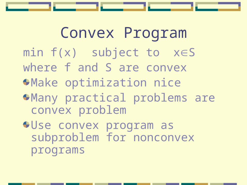
Convex Programmin f(x) subject to xSwhere f and S are convex

Make optimization niceMany practical problems are convex problemUse convex program as subproblem for nonconvex programs

Theorem : Global Solution of convex program

If x* is a local minimizer of a convex programming problem, x* is also a global minimizer. Further more if the objective is strictly convex then x* is the unique global minimizer.

Proof:

contradiction x*

yf(y)<f(x*)

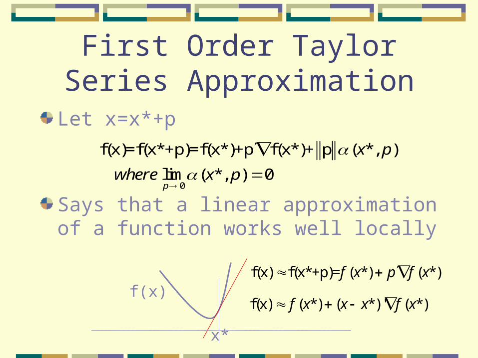
First Order Taylor Series Approximation

Let x=x*+p

Says that a linear approximation of a function works well locally

0

f(x)=f(x*+p)=f(x*)+p f(x*)+ p ( *, )

lim ( *, ) 0p

x p

where x p

f(x) f(x) f(x*+p)= ( *) ( *)f x p f x

x*

f(x) ( *) ( *) ' ( *)f x x x f x

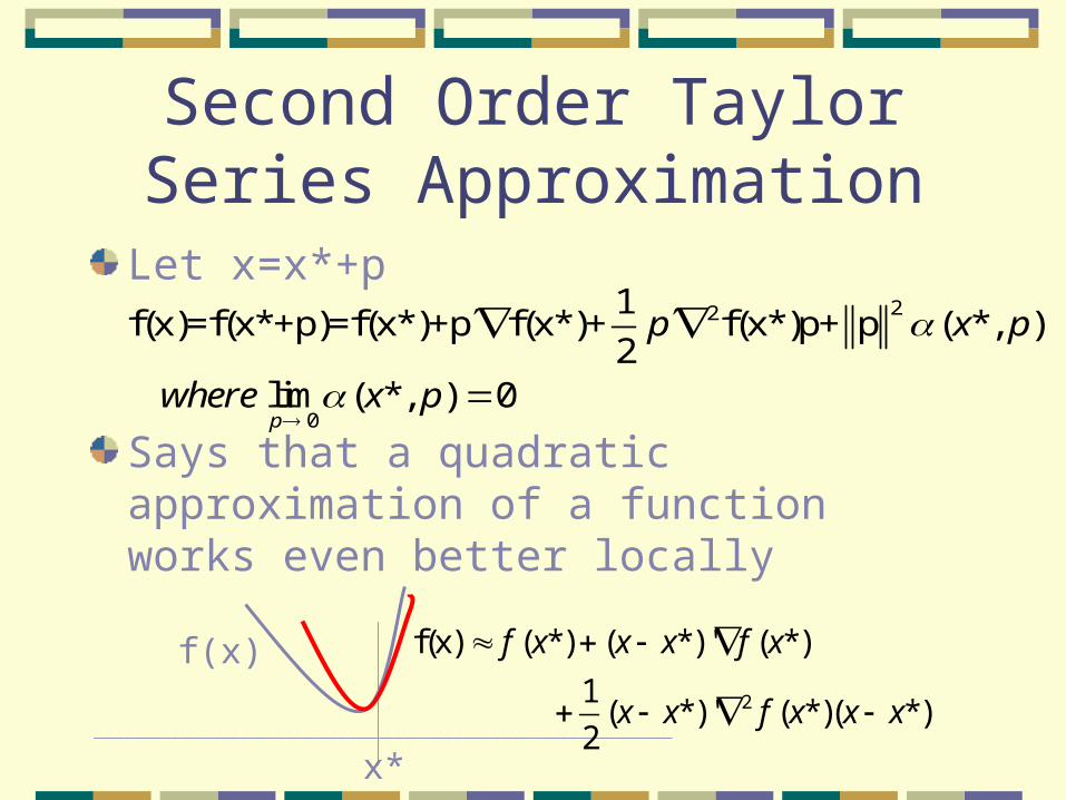
Second Order Taylor Series Approximation

Let x=x*+p

Says that a quadratic approximation of a function works even better locally

22

0

1 f(x)=f(x*+p)=f(x*)+p f(x*)+ f(x*)p+ p ( *, )

2lim ( *, ) 0p

p x p

where x p

x*

f(x)2

f(x) ( *) ( *) ' ( *)

1( *) ' ( *)( *)

2

f x x x f x

x x f x x x

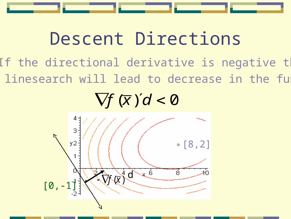
Descent Directions If the directional derivative is negative then

linesearch will lead to decrease in the function

[8,2]

[0,-1]d

( ) 0f x d

( )f x

First Order Necessary Conditions

Theorem: Let f be continuously differentiable.

If x* is a local minimizer of (1),

then

( *) 0f x

Second Order Sufficient Conditions

Theorem: Let f be twice continuously differentiable.

If and

then x* is a strict local minimizer of (1).

( *) 0f x

2 ( *) is positive definitef x

Second Order Necessary Conditions

Theorem: Let f be twice continuously differentiable.

If x* is a local minimizer of (1)

then

( *) 0f x

2 ( *) is positive semi definitef x

Optimality Conditions

First Order Necessary

Second Order Necessary

Second Order Sufficient

With convexity the necessary conditions become sufficient.

Easiest Problem Line Search =

1-D Optimization

Optimality conditions based on first and second derivatives

Golden section search

: [ , ]

min ( ) . . [ , ]

f a b R

f x s t x a b S

(1)

Sometimes can solve linesearch exactly

The exact stepsize can be found

min ( ) ( )

'( ) ' ( ) 0

g f x d

g d f x d

General Optimization algorithm

Specify some initial guess x0

For k = 0, 1, …… If xk is optimal then stopDetermine descent direction pk

Determine improved estimate of the solution: xk+1=xk+kpk

Last step is one-dimensional search problem called line search

Newton’s Method

Minimizing quadratic has closed form

1

2

1

( )

( ) 0

Minimum must satisfy, *

* (unique if Q is invertible)

g x x Qx b x

g x Qx b

Qx b

x Q b

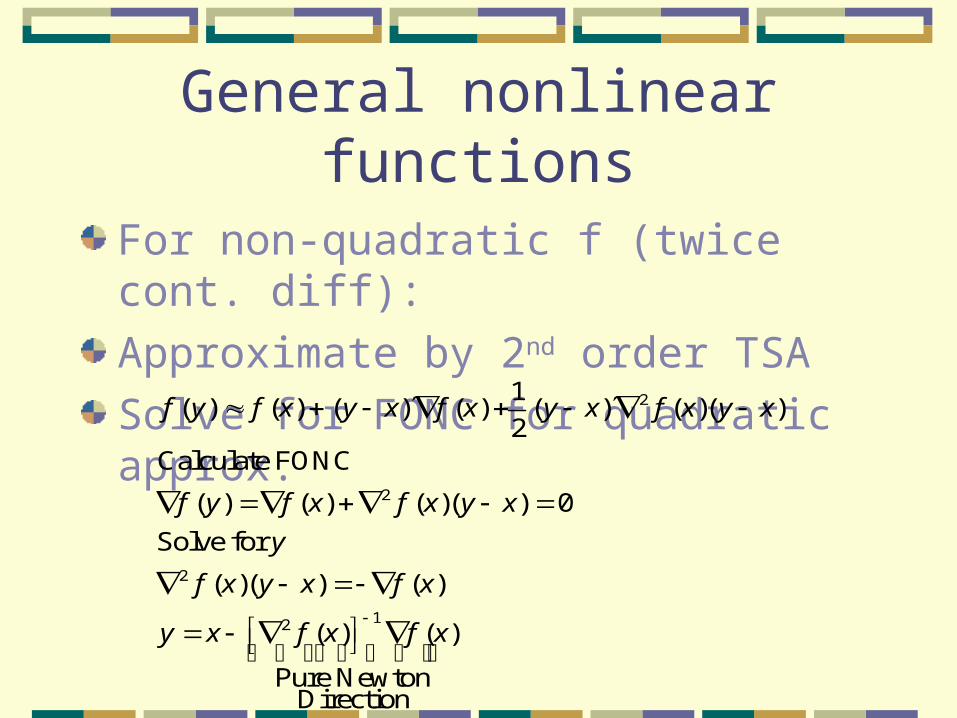
General nonlinear functions

For non-quadratic f (twice cont. diff):

Approximate by 2nd order TSA

Solve for FONC for quadratic approx.2

2

2

12

1( ) ( ) ( ) ( ) ( ) ( )( )

2Calculate FONC

( ) ( ) ( )( ) 0

Solve for

( )( ) ( )

( ) ( )

Pure Newton Direction

f y f x y x f x y x f x y x

f y f x f x y x

y

f x y x f x

y x f x f x

Basic Newton’s Algorithm

Start with x0

For k =1,…,K If xk is optimal then stopSolve:Xk+1=xk+p

2 ( ) ( )k kf x p f x

Final Newton’s Algorithm

Start with x0

For k =1,…,K If xk is optimal then stop Solve:

using modified cholesky

factorization Perform linesearch to determine

Xk+1=xk+kpk

2 ( ) 'kf x E LDL ' ( )k kLDL p f x

What are pros and cons?

Steepest Descent Algorithm

Start with x0

For k =1,…,K If xk is optimal then stop

Perform exact or backtracking linesearch to determine

xk+1=xk+kpk

( )k kp f x

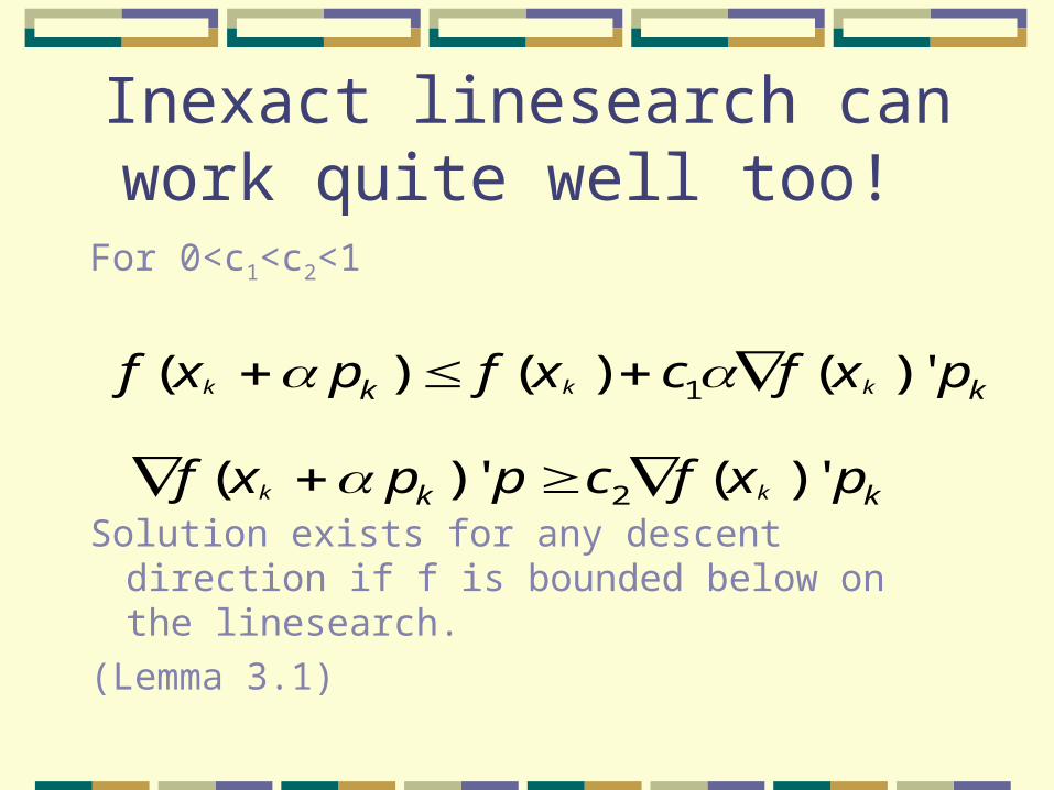
Inexact linesearch can work quite well too!

For 0<c1<c2<1

Solution exists for any descent direction if f is bounded below on the linesearch.

(Lemma 3.1)

1( ) ( ) ( ) 'k k kk kf x p f x c f x p

2( ) ' ( ) 'k kk kf x p p c f x p

Conditioning Important for gradient methods!

50(x-10)^2+y^2Cond num =50/1=50

Steepest DescentZIGZAGS!!!

Know Pros and Cons of each approach

Conjugate Gradient (CG)

Method for minimizing quadratic function

Low storage method

CG only stores vector information

CG superlinear convergence for nice problems or when properly scaled

Great for solving QP subproblems

Quasi Newton MethodsPros and Cons

Globally converges to a local min

always find descent direction

Superlinear convergence

Requires only first order information – approximates Hessian

More complicated than steepest descent

Requires sophisticated linear algebra

Have to watch out for numerical error

Quasi Newton MethodsPros and Cons

Globally converges to a local minSuperlinear convergence w/o computing HessianWorks great in practice. Widely used. More complicated than steepest descentBest implementations require sophisticated linear algebra, linesearch, dealing with curvature conditions. Have to watch out for numerical error.

Trust Region Methods

Alternative to line search methods

Optimize quadratic model of objective within the “trust region”

)(xf

ix1ix

k

kiik

pts

pBppxfxfp

..

'2

1)'()(minarg

Easiest Problem

Linear equality constraints

min ( )

. . ,

n

m n m

f x f R

s t Ax b A R b R

Lemma 14.1 Necessary Conditions (Nash + Sofer)

If x* is a local min of f over {x|Ax=b}, and Z is a null matrix

Or equivalently use KKT Conditions

2

' ( *) 0

' ( *) . . .

Z f x

and Z f x Z is p s d

2

( *) ' 0

*

' ( *) . . .

f x Ahas a solution

Ax b

Z f x Z is p s d

Other conditionsGeneralize similarly

Handy ways to compute Null Space

Variable Reduction Method

Orthogonal Projection Matrix

QR factorization (best numerically)

Z=Null(A) in matlab

Next Easiest Problem

Linear equality constraints

Constraints form a polyhedron

min ( )

. . ,

n

m n m

f x f R

s t Ax b A R b R

Polyhedron Ax>=b

( *) *

*

( * ) 0

0

Ti i

i

i i i

f x A a

Ax b

A x b

a1x = b1

*)(xf

a1

Inequality Case

a4x = b4

a3x = b3

a5x = b5

a2x =b5

a2

Inequality problem

Nonnegative Multipliers imply gradient points to the greater thanSide of the constraint.

x*

* min ( )

. .

1...i i

x f x

s t a x b

i d

Inequality FONC:

Second Order Sufficient Conditions for Linear

InequalitiesIf (x*,*) satisfies

2

* Primal feasibility

( *) ' * Dual feasibility

* 0

*'( * ) 0 Complementarity

and SOSC ' ( *) . .

Then x* is a strict local minimizer

Ax b

f x A

Ax b

Z f x Z is p d

Sufficient Conditions for Linear Inequalities

where Z+ is a basis matrix for Null(A

+) and A + corresponds to nondegenerate active constraints)

i.e.+

*j

A

{ | * , 0 }

J

j j

A

j A x b

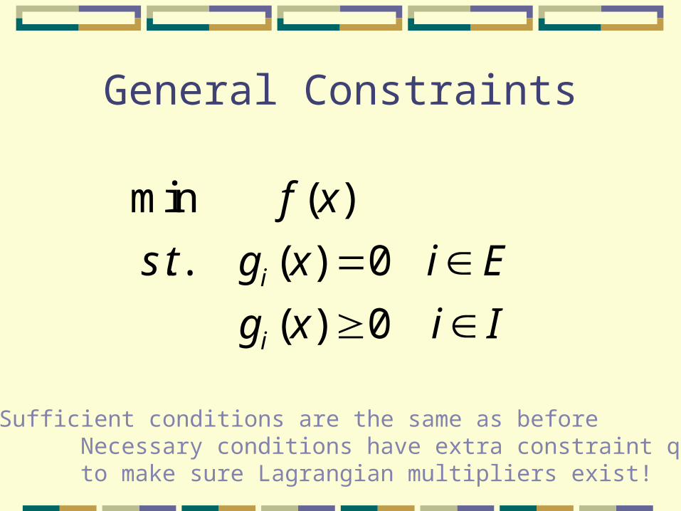
General Constraints

min ( )

. . ( ) 0

( ) 0i

i

f x

s t g x i E

g x i I

Careful : Sufficient conditions are the same as before Necessary conditions have extra constraint qualification to make sure Lagrangian multipliers exist!

Necessary Conditions General

If x* satisfies LICQ and is a local min of f over {x|g(x)>=0,h(x)=0}, * *

* *

'

2

there exists 0,

0 ( *, *, *) ( *) ( *) ( *)

( *) 0 , ( *) 0

* ( *) 0

' ( *) . .

is the null space matrix for ( *) (active

constraints)

I E

x I E i i i ii i

xx

L x f x g x h x

g x h x

g x

and Z L x Z is p s d

where Z A x

Algorithms build on prior Approaches

Linear Equality Constrained: Convert to unconstrained

and solvemin ( )f x

min ( )

. .

f x

s t Ax b

Different ways to representNull space produceAlgorithms in practice

Prior Approaches (cont)

Linear Inequality Constrained: Identify active constraints

Solve equality constrained

subproblems

Nonlinear Inequality Constrained: Linearize constraints Solve subproblems

min ( )

. .

f x

s t Ax b

min ( )

. . ( ) 0

f x

s t g x

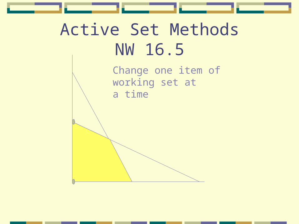
Change one item of working set at a time

Active Set MethodsNW 16.5

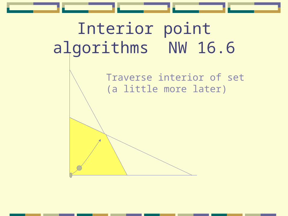
Traverse interior of set (a little more later)

Interior point algorithms NW 16.6

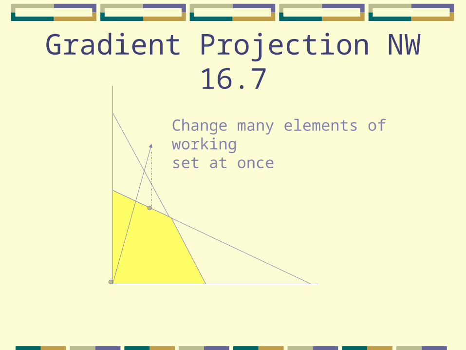
Change many elements of working set at once

Gradient Projection NW 16.7

Generic inexact penalty problem

min ( )

( ) . . ( ) 0

( ) 0i

i

f x

NLP s t g x i E

g x i I

2 2( , ) ( ) ( ( )) (( ( )) )i ii E i I

P x f x g x g x

From

To

What are penalty problems and why do we use them?Difference between exact and inexact penalties.

Augmented Lagrangian

Consider min f(x) s.t h(x)=0

Start with L(x, )=f(x)-’h(x)

Add penalty

L(x, ,c)=f(x)-’h(x)+μ/2||h(x)||2

The penalty helps insure that the point is feasible.

Why do we like these? How do they work in practice?

Sequential Quadratic Programming (SQP)

Basic Idea:QP with constraints are easy. For any

guess of active constraints, just have to solve system of equations.

So why not solve general problem as a series of constrained QPs.

Which QP should be used?

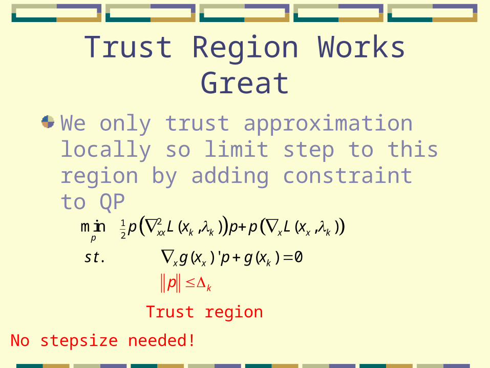
Trust Region Works Great

We only trust approximation locally so limit step to this region by adding constraint to QP

21

2min ' ( , ) ' ( , )

. . ( ) ' ( ) 0

xx k k x x kp

x x k

k

p L x p p L x

p

s t g x p g x

Trust region

No stepsize needed!

Advanced topics

Duality Theory – Can choose to solve primal or dual

problem. Dual is always nice. But there may be a “duality gap” if overall

problem is not nice. Nonsmooth optimization

Can do the whole thing again on the basis of subgradients instead of gradients.

Subgradient

Generalization of the gradient

Definition

at x. oft subgradien a is

x)-(yg' f(x)f(y)

such that g vector a

function.convex a be:Let

f

R

RRfn

n

Hinge loss

0 1f(y) f(x) g'(y-x)