Review and Enhancement of CHART Operations to …attap.umd.edu/wp-content/uploads/2015/09/MD-12-SP009B4U... · 2015-09-29 · REVIEW AND ENHANCEMENT OF CHART OPERATIONS TO MAXIMIZE

STATE HIGHWAY ADMINISTRATION

RESEARCH REPORT

REVIEW AND ENHANCEMENT OF CHART OPERATIONS TO MAXIMIZE THE BENEFITS OF INCIDENT RESPONSE AND

MANAGEMENT

WOON KIM AND GANG-LEN CHANG

DEPARTMENT OF CIVIL AND ENVIRONMENTAL ENGINEERING

UNIVERSITY OF MARYLAND COLLEGE PARK, MD 20742

SB009B4U FINAL REPORT

JULY 2012

Martin O’Malley, Governor Beverley K. Swaim-Staley, Secretary Anthony G. Brown, Lt. Governor Melinda B. Peters, Administrator

MD-12- SB009B4U

The contents of this report reflect the views of the author who is responsible for the facts

and the accuracy of the data presented herein. The contents do not necessarily reflect

the official views or policies of the Maryland State Highway Administration. This report

does not constitute a standard, specification, or regulation.

ii

Technical Report Documentation PageReport No. MD-12- SB009B4U

2. Government Accession No. 3. Recipient's Catalog No.

4. Title and Subtitle Review and Enhancement of CHART Operations to Maximize the Benefit of Incident Response and Management

5. Report Date July 2012 6. Performing Organization Code

7. Author/s

Woon Kim and Gang-Len Chang

8. Performing Organization Report No.

9. Performing Organization Name and Address University of Maryland, Department of Civil and Environmental Engineering, Maryland, College Park, MD 20742

10. Work Unit No. (TRAIS)

11. Contract or Grant No. SP009B4U

12. Sponsoring Organization Name and Address Maryland State Highway Administration Office of Policy & Research 707 North Calvert Street Baltimore, MD 21202

13. Type of Report and Period Covered Final Report 14. Sponsoring Agency Code (7120) STMD - MDOT/SHA

15. Supplementary Notes 16. Abstract

This project was focused on identifying potential areas for Maryland’s Coordinated Highway Action Response Team (CHART) to enhance its incident management efficiency and to maximize the resulting benefits under existing resource constraints. Using the information from CHART and the Maryland Accident Analysis Reporting System (MAARS), this research has identified critical factors affecting CHART’s efficiency in incident response and clearance, and produced several reliable models to improve its performance. This research has also produced an optimal allocation model that will enable each operational center to best deploy available patrol vehicles along its responsible highway networks and to select the most cost-benefit fleet size under the resource constraints.

CHART can also apply the set of prediction models developed in this project to estimate the

required clearance duration of a detected incident, thereby minimizing the resulting congestion within the impact boundaries via some real-time traffic control and information strategies. Incorporating any of those developed models into current practice will undoubtedly enhance CHART’s operational quality and significantly increase its effectiveness in minimizing non-recurrent congestion in this region. 17. Key Words Incident, CHART, benefits, clearance time

18. Distribution Statement: No restrictions This document is available from the Research Division upon request.

19. Security Classification (of this report) None

20. Security Classification (of this page) None

21. No. Of Pages 75

22. Price

Form DOT F 1700.7 (8-72) Reproduction of form and completed page is authorized.

iii

Table of Contents

CHAPTER 1: Introduction ................................................................................................. 1

1.1 Research Background ............................................................................................... 1

1.2 Research Objective and Work Plan .......................................................................... 2

1.3 Report Organization .................................................................................................. 2

CHAPTER 2: Exploring Accident Data Integration between CHART and MARRS ........ 5

2.1 Introduction ............................................................................................................... 5

2.2 Data Items for Integrating Accident Information ..................................................... 5

2.3 Matching Results and Recommendations ................................................................. 9

CHAPTER 3: Review of Incident Response Efficiency ................................................... 11

3.1 Introduction ............................................................................................................. 11

3.2 Distribution of Incident Response Times by Key Factors ...................................... 12

3.3 Performance between Different Operations Centers .............................................. 15

3.4 Summary of Key Research Findings ...................................................................... 18

CHAPTER 4: Analysis of Incident Clearance Efficiency ................................................ 20

4.1 Introduction ............................................................................................................. 20

4.2 Distribution of Incident Clearance Times by Critical Factors ................................ 20

4.3 Analysis of Incident Clearance Efficiency by Operations Center .......................... 23

4.4 Research Findings and Conclusions ....................................................................... 27

CHAPTER 5: A Real-Time Model for Predicting Incident Clearance Duration ............. 29

5.1 Introduction ............................................................................................................. 29

5.2 Literature Review.................................................................................................... 29

5.3 Analysis of Prediction Algorithms.......................................................................... 31

5.4 Model Development and Estimation Results .......................................................... 35

iv

5.5 Conclusion .............................................................................................................. 46

CHAPTER 6: Optimal Strategies for Deploying Freeway Incident Response Units ....... 48

6.1 Introduction ............................................................................................................. 48

6.2 Review of available models .................................................................................... 48

6.3 Model Formulation ................................................................................................. 51

6.4 Numerical results .................................................................................................... 55

CHAPTER 7: Conclusions ............................................................................................... 67

7.1 Conclusions ............................................................................................................. 67

7.2 Recommendations ................................................................................................... 69

References ......................................................................................................................... 72

1

CHAPTER 1: Introduction

1.1 Research Background

Although the contribution of the emergency response operations of Maryland’s

Coordinated Highway Action Response Team (CHART) has been well recognized by the general

public, much remains to be done to effectively contend with increasingly congested traffic

conditions and the accompanying incidents. In fact, to meet the expectation of policymakers and

residents on minimizing the impact of non-recurrent congestion, CHART operations inevitably

face the following challenges:

• How to increase its detection coverage and rate?

• Can the incident response time be further reduced?

• How can the incident clearance operations be performed more efficiently?

• How can the overall performance of CHART be maximized under the current resource

constraints?

The performance evaluations of CHART, conducted by The University of Maryland

research team annually over the past 10 years, indicate that even a small percentage of

improvement on any of the above challenging areas could increase benefits significantly. One

potentially effective way to contend with such challenges is to take advantage of valuable

information embedded in the CHART operational record over the past several years. For

example, an in-depth comparison of CHART incident data and MAARS reports (i.e., Maryland

Automated Accident Report System) can shed some light on why some incidents were not

recorded by CHART. Such information can then be used to design some reliable ways to expand

CHART’s detection coverage.

A rigorous investigation of the relations between the incident clearance time and all

contributing factors from the past data may explain why some types of incidents often result in

longer durations, thus degrading the performance of CHART’s response operations. From the

spatial distribution of incidents over different times of day in each target highway network over

the past several years, CHART can also better allocate its highway patrol units to minimize

incident response times. In addition, the analysis of CHART’s performance as a function of its

available budget may also assist responsible staff to justify the needed resources.

2

Considering the ever-increased statewide congestion and the demanding expectation of

motorists, CHART will inevitably face the challenge of sustaining its impressive performance

with diminishing resources. Thus, it is essential that CHART can maximize its effectiveness and

efficiency by learning from the past operational experiences.

1.2 Research Objective and Work Plan

The primary project objective is to develop some effective strategies that can assist

CHART staff in improving the efficiency of its operations and maximizing the resulting benefits

under the existing resource constraints. Strategy development due to data constraints has

focused on the following critical aspects:

• Understanding critical factors that contribute to an increase in incident response and

clearance times;

• Allocating available highway patrol units based on the temporal and spatial distributions

of incidents to minimize the potential incident response times; and

• Developing reliable models to predict the required duration of a detected incident and to

identify critical contributing factors.

Based on the above research objective, the project work was divided into two parts: Part-I

was concentrated on the analysis of CHART’s performance data from 2007-2009 to identify

potential improvement areas and Part-II was devoted to developing operational models to

minimize incident response and clearance times. The study also includes recommendations for

CHART’s enhancement of incident response and traffic management.

1.3 Report Organization

This research report comprises six chapters. A brief description of core research results

in each chapter is presented below.

Chapter 2 presents the exploratory results of integrating accident records reported

independently to CHART and MAARS. Section 2-1 first illustrates key variables and data items

used by CHART to characterize a responded accident, followed by identification of similar data

in MAARS recorded by the State Police Department for the same response operations. Section 2-

2 describes a data fusion process to select key variables from these two databases for integrating

3

critical information associated with the same accidents. This section also details the criteria and

sequential search process used to match accident records between these two databases. Section 2-

3 reports the data integration results and recommendations for best using information from these

two databases.

Chapter 3 documents the analysis results of CHART’s incident response efficiency

between 2007 and 2009, focusing on the interrelationships between incident response time and

all contributing factors. Section 3-1 presents the distribution of incident response times classified

by the number of blocked lanes and incident nature, finding that CHART patrol units tend to

respond more quickly to more severe incidents. Section 3-2 compares the performance of each

operational center in response to different types of incidents, times of day, and environmental

conditions. The comparison also includes the performance discrepancies among five CHART

operational centers during peak and off-peak periods on different highways, highlighting the

impacts of traffic congestion on the efficiency of incident response. Section 3-3 summarizes

research findings and recommendations for improving the efficiency of incident response.

Chapter 4 details critical factors affecting each traffic control center’s efficiency in

recovering traffic from incidents, highlighting the complex compound impacts of the incident’s

nature, lane blockage, and environmental conditions on the resulting incident clearance time.

Section 4-1 presents the distribution of average clearance times by blocked lanes, incident

severity, and heavy vehicle involvement. This section also illustrates the correlations between

incidents of excessively long duration (i.e., over two hours) and the number of fatalities and

injuries. Section 4-2 evaluates the performance of five CHART operation centers, focusing on

their efficiency in clearing various types of lane-blockage incidents at different times of day and

in severe weather conditions. Section 4-3 summarizes the research findings and identifies

critical variables for developing a prediction model for incident clearance time.

Chapter 5 reports on the efforts to develop a set of reliable models for predicting duration

of incident clearance, based on the dataset integrated from CHART and MAARS. Section 5-2

offers a concise review of related literature, including a selection of explanatory variables and a

discussion of critical issues associated with model development. Section 5-3 illustrates the core

logic of various Bayesian-based estimation models, highlighting their strengths in modeling the

unique characteristics of incident clearance time. Section 5-4 reports the estimation results from

various incident clearance models calibrated with the merged dataset from the CHART and

4

MAARS databases. Section 5-5 includes research findings and recommendations for developing

a comprehensive model to predict incident duration in the future.

Chapter 6 discusses various optimization strategies for SHA to effectively distribute

incident response units along freeway segments plagued by frequent incidents, including a

comparison between the models developed from this research and other state-of-the practice

deployment strategies, using the incident data from 2006 to 2011 on the I-495 Capital Beltway.

Section 6-2 reviews the available strategies for deploying emergency response units and

relevant studies in the literature. Section 6-3 analyzes the formulations of several promising

deployment models, including the one developed from this project. Section 6-4 illustrates a

comprehensive benefit/cost analysis with different response fleet sizes. Research findings

produced from extensive analyses of the developed model are summarized in the last section,

providing a basis for traffic managers to design a benefit-cost incident management system.

Chapter 7 summarizes the research findings of this project and recommends some areas

essential for CHART’s performance improvement, especially for incidents resulting in injuries

and fatalities. Some critical issues associated with field data collection and management of the

incident database are also discussed in this chapter.

5

CHAPTER 2: Exploring Accident Data Integration between CHART and

MARRS

2.1 Introduction

Both CHART and the Maryland State Police (MSP) record related information for their

respective analyses. However, due to the differences in responsibility, each agency records

mainly those data related to its potential applications, making the identification of contributing

factors to accidents and their relations with the surrounding traffic conditions a very difficult

task. This chapter presents comparisons of accident information recorded in CHART’s database

and MARRS (Maryland Automated Accident Record System), focusing on inconsistencies

between these two databases and potential methods for their future integration.

This chapter is organized as follows: section 2.2 describes the format used by each

database for recording accident-related information, and the list of key variables to characterize a

recorded accident. Section 2.3 illustrates the data fusion process between these two databases

and the matching results based on accident records from 2006 to 2008. Section 2.4 summarizes

the suggestions for CHART and MAARS to form a complete accident information system for

various operations and safety analyses.

2.2 Data Items for Integrating Accident Information

The exploratory analysis was intended to find an effective way to match the recorded

accidents between CHART and MAARS, as the injury and fatality information available only in

the latter is critical to the development of prediction models for incident duration. The

experimental analysis started with the MAARS data from 2006 to 2008, where 103,510 accident

records were identified for integration. Over the same period, CHART’s database contained

6,053 incident records involving either injuries or fatalities. Table 2-1 shows the list of data

fields from CHART for use to match with the same accidents in MAARS.

6

Table 2-1: Data fields from CHART for use to match with MAARS

Field Name Example Datum event_id 8d00488a2c5900e10047832e33235daa

county code 11 direction_code 2

event_open_date 3/19/2008 14:20 event_closed_date 3/19/2008 16:24

location_text US 15 NORTH AT OLD FREDERICK RD cpi 1 cf 1

total_num_veh 2 route_number 15 route_prefix US

Note that the fields of “route_number” and “route_prefix” were not originally present in

the database, so they had to be generated by searching “location_text”. More than 40 fields in

CHART’s database were excluded from the table for accident matching, since they have no

corresponding analogues in MAARS. The field “cpi” stands for “collision and personal injury,”

while “cf” stands for “collision and fatality.” The field “direction_code” represents the direction

of the traffic on the side of the road where the incident occurred, which is not always the road’s

official cardinal direction, and mostly tends to be the approximate tangential direction of the road

at that location.

Table 2-2 presents the related data fields in MAARS used to match those in Table 2-1

from CHART’s database. Different from the information contained in MAARS’s original field,

the “Acc_date” field shown in the table has been aggregated with a special program to include

both the accident date and time. The field of “total_num_veh” from CHART (see Table 2-1)

corresponds to the “NO_veh”, as they represent the number of vehicles involved in the incident.

The “Route_NO” and “Route_Type correspond to “route_number” and “route_prefix” in

CHART, respectively, and represent the road where the incident occurred.

The criteria used to match accidents in these two databases include:

1. The logging date and time of the incident;

2. Information on the location of the incident;

3. The number of vehicles involved in the incident; and

7

4. Whether the incident resulted in injury only, fatality, or both.

Note that the first two matching criteria would be sufficient to identify the same accidents

for data integration if relevant information has been recorded properly in both databases.

However, due to the discrepancy in the accident logging time between these two databases,

criteria 3 and 4 were further used to ensure a better match. For logging date and time, the

event_open_date table column from CHART’s database was chosen, because that particular

column represents the earliest logging timestamp of the recorded incident. The columns titled

Acc_Date and Acc_Time, from MAARS were combined to form a similar earliest-logging-

timestamp column. Criterion 3 was proposed because both databases contained a similar column

to denote the number of vehicles involved.

Table 2-2: Data fields from MAARS for use to match with CHART

Field Name Example Datum Report_NO 809878892

County 10 Route_NO 15

Route_Type US Final_log_mile 35.02

Acc_date 3/19/2008 14:05 Inter_NO

NO_ped_injured 0 NO_ped_killed 0

NO_doc_injured 2 NO_doc_killed 1

NO_veh 2 Chart_county_code 11

To compile the information on the location of the incident, several columns were used

from each database. For example, the original CHART database represents the county name of

the accident location as a numeric code and uses a direction code to indicate the blocked traffic

direction, (i.e., Southward or Northward), and a text-based location column that in many cases

follows the format of “<route prefix and number or street name> AT/PRIOR/AFTER

<identifying feature or intersection>”. Some examples of variations in location format from

CHART’s database are shown in Table 2-3.

8

Table 2-3: Examples of accident location information recorded in CHART’s database

Location_text Event_id US 15 @ SUNDAYS LANE 0000bc0a5298006d0046b48c33235daa

~I-495 / I-95 AT MD 214 CENTRAL AVE 1800116c0ebd00ed0046b48c33235daa md 424 at bell branch 28ff35b03f85009d0045b48c33235daa

Because of these inconsistencies, this study has produced a computer program to parse

the route prefixes and route numbers from 6,024 of the 6,053 CHART records. The resulting

accuracy has been verified by the research team members with a manual matching method.

In contrast, the location information in MAARS was already split into the fields of

Route_Type, Route_No, Final_Log_Mile, Inter_No, which are, respectively route prefix, route

number, mile along the route from the beginning of the route in each county, and the intersection

number. Unfortunately, the intersection number was left blank in most sample records and,

therefore, cannot be used to pinpoint the location of the incident along the route.

The attempt to use the field of Final_Log_Mile was not successful because of the

inconsistency in data recording. For example, some event records used one location in a county

as “beginning of the route” and the other point as the “end,” but other records used the same pair

of locations in a reverse order, thus making the information unusable to identify the accident

location. Hence, the data matching with the accident location was based mainly on county codes,

route prefixes, and route numbers. Note that ideally the matching process between these two

databases can still yield acceptable results using the information from these fields, especially if

the logging of the accident times was accurately recorded.

The procedures used to perform the accident data matching are summarized below:

Step-1: For each record in the CHART record set, a matching record was searched in MAARS

with the information fields of county, route prefix, and route number, as well as injury- or

fatality-related data and vehicle number.

Step-2: For those matched accident records produced by Step-1, the logging timestamp of each

CHART incident record with a time window of 30 minutes (+ 15 minutes) was used

subsequently to filter those identified records.

Step-3: After excluding all records that were already matched, the same procedures were

reapplied to the remaining data records in MAARS but with a wider time window (i.e.,

+1 minute per increment).

Step-4: Repeat Step-1 to Step-3 until the time window reaches 60 minutes (+30 minutes).

9

Note that filtering the accident records with a small time-bound increment was to ensure

the best possible match based on the available criteria. After the time window reached 60

minutes (i.e., the preset limit), the matching criteria were revised to include those records where

their accident-involved vehicles recorded by two databases differ by one. This decision was

based on the assumption that either the CHART’s response unit or the highway police could

arrive at the accident scene later than the other party and was not notified that a vehicle had

already been towed.

To increase the matched samples, the filtering process was further loosened to include

those accident records in the two databases that meet all matching criteria except the

injury/fatality information. This approach was proposed to account for some scenarios when

victims could die in the hospital and either of these two parties failed to receive an update and

thus recorded a different number of injuries and fatalities.

Note that double-matching was not an issue with this procedure. Every round of search

produced only a few (less than 50) new records, and every record in the MAARS’s database

yielded either one or no match with accident records in the CHART’s database. The data search

procedures were stopped at the time window of 60 minutes, because it was difficulty to verify

that those accidents recorded in these two databases beyond the 60-minute (+30 minutes)

window were indeed the same accidents.

2.3 Matching Results and Recommendations

Using the above procedures, the final matched data set between these two accident

databases included only 1,930 of the 6,024 possible records, or about 32 percent. This result is

disappointing and highlights the need to address this vital data integration issue.

Some recommendations on how to address this imperative task are summarized below.

• For the CHART’s database, the location_text field should be separated into a

route_prefix, route_number, and intersecting_route_prefix, intersecting_route_number.

The route number and intersecting route number should be strictly number-based.

• MAARS’s database has the information on county roads and their route numbers, so the

same data should be shared with CHART to log those incidents that occurred on county

roads.

10

• The route_prefix and intersecting_route_prefix should be either code-based, (i.e., 0 = IS,

1 = US, 2 = MD, 3 = CO), or should be restricted to an enumerated data type that allows

the user to select only IS, US, MD, or CO. If the accident does not occur at an

intersection, the intersecting_route_number and intersecting_route_prefix should be left

blank.

• Both CHART and MAARS should use a precise geographical coordinate obtained via

GPS to pinpoint the exact location of every reported incident. By doing so, both

databases can produce more reliable information than with a text-based reference to any

special landmark or feature, such as “Howard County Border” or “Fort McHenry Toll

Plaza.”

Note that the use of GPS location information will be operationally more convenient than

logging the mile marker along the road that may not exist, especially for smaller roads. GPS

information can also prevent the confusion of logging the miles along the road from the

beginning of a county, because it is often not clear how to measure or which point to use as the

“beginning.” Recording the accident location with such information would also allow potential

users to match the incidents by location between the two databases by placing a certain radial

constraint on the coordinates.

Recognizing the practical difficulties in changing the data recording procedures and

formats for CHART and MAARS, the above minor modifications if properly implemented,

however, can significantly increase the matching results between these two systems, even with

the remaining recording discrepancies. The information integrated from these two databases

systems will be very useful for enhancing CHART’s operational performance and developing

safety improvement programs for highway networks in this region.

11

CHAPTER 3: Review of Incident Response Efficiency

3.1 Introduction

This chapter presents the analysis results of CHART’s response efficiency to different

types of incidents, focusing on identifying key factors that often cause excessively long response

times. It is expected that an in-depth analysis of the interrelationships between incident patterns

and the performance of each local operational center under various environmental and traffic

conditions can reveal some critical areas for SHA to further improve its operational strategies in

contending with non-recurrent traffic congestion.

The rest of this chapter is organized as follow: Section 3-2 illustrates the distribution of

incident response duration by critical factors such as the number of blocked lanes and fatalities,

using the CHART incident data from 2007 to 2009. Section 3-3 compares the efficiency of

CHART’s five local response centers in response to various types of incidents, highlighting their

performance discrepancies under the resource constraints and the responsible network coverage.

Research findings and suggestions constitute the last section. Figure 3-1 illustrates the definition

of each technical term and its corresponding timeline in the entire incident response and

clearance process.

Figure 3-1: Graphical illustration of the entire incident response and clearance process

12

3.2 Distribution of Incident Response Times by Key Factors

Figure 3-2 presents the distribution of CHART’s average incident response times by

whether or not incidents resulted in lane blockage and fatalities. During this 3-year period (2007-

2009), CHART’s average response times to incidents involving lane blockage were quicker than

those causing only shoulder-lane rubbernecking impact. Similar discrepancy patterns also exist

between incidents involving fatalities and those causing only injuries or property damage. The

exact factors contributing to such performance discrepancies are to be identified by CHART, but

the resource limitations and/or personnel constraints may naturally make incident response units

to give a higher priority to those incidents potentially causing greater traffic impacts.

Figure 3-2: Comparisons of incident response times between with and without causing lane

blockage, and with and without resulting in fatalities.

Figure 3-3 further compares the response time discrepancy under the following

classifications:

• On five major commuting freeway corridors: I-270, I-495, I-70, I-695, I-95.

• On incidents of different severity levels: disabled vehicles, property damage, injury, and

fatality.

13

• On different pavement conditions: snowy, wet, and dry, during peak and off-peak

periods.

• By different response centers.

As shown in the graphical patterns, the finding that incidents involving lane blockage

have shorter response times than those with no lane blockage holds across different roads, injury

severities, pavement conditions, and times of the day.

Figure 3-3: Comparisons of incident response times between with and without causing lane

blockage across different classifications

Figure 3-4 shows the comparison of average response times between incidents under

different pavement conditions. As expected, severe weather conditions such as snow and ice

indeed increased the average response time, reflecting the need to have special preparations to

respond to incidents occurring on such days.

14

Figure 3-4: Comparison of incident response times with and without snow/ice conditions

Figure 3-5 further illustrates the impacts of traffic congestion on the average incident

response time, reflecting the need to prevent the response team from being impeded by slow

traffic during peak hours. For example, it took CHART’s response units in the Washington

region an average of 10.5 minutes to reach an incident scene if no lane blockage occurred during

peak periods, but only 7.4 minutes for the same type of incidents during off-peak periods.

Similarly, it took the response team in the Baltimore region an average of 10 minutes and 7.5

minutes, respectively, for the same incident type during peak and off-peak periods. This finding

also holds for incidents of different severities across all CHART’s service regions. It, however,

is noticeable that CHART’s response efficiency varies with incident severity and its resulting

traffic impact (i.e. number of blocked lanes) regardless of the roadway congestion. This finding

is evidenced in the consistent pattern shown in Figure 3-5.

15

Figure 3-5: Average response time by region during peak and non-peak periods

3.3 Performance between Different Operations Centers

Due in part to the available resources, the response efficiency of CHART’s five

operations centers varies significantly, where AOC generally outperforms all other centers and

TOC7 tends to take the longest response time for the same type of incidents. A graphical

comparison of the average response times among these five centers to incidents with and without

resulting lane blockage is shown in Figure 3-6. Table 3-1 further shows the performance

discrepancy among those centers even responding to incidents on the same route. For example,

TOC7 took an average of 9.8 minutes to respond to incidents on I-70, longer than 6.5 minutes by

SOC and 7.3 minutes by TOC3. Similarly, the average response time for AOC to reach incident

scenes on I-95 was 4.5 minutes, about 40 percent less than TOC3 (i.e., 8.4 minutes).

Understandably, various factors could contribute to these performance discrepancies. However,

ensuring the consistency of incident response efficiency across different service regions is an

important issue for CHART.

16

Figure 3-6: Comparison of average response times among five operations centers

Table 3-1: Comparison of incident response times between response centers on different roads

Center I-70 I-270 I-95 Mean St. D* N** Mean St. D N Mean St. D N

TOC7 9.8 6.6 198 9.0 5.6 362 TOC3 7.3 6.4 290 8.4 6.8 166 TOC4 6.8 5.4 290 7.6 5.4 212 SOC 6.5 7.3 63 4.7 5.3 34 6.1 7.4 113 AOC 4.5 5.2 2249

*standard deviation; ** sample size

Table 3-2 further compares the performance of those five response centers in response to

incidents causing no fatality during the off-peak period. As reflected in the statistics, TOC7, on

average, took 16.4 minutes on a snowy day to respond to an incident causing no lane blockage

and fatality. This is much longer than the average 11 minutes to respond under the same

conditions but without snow. In contrast, AOC’s response times to the same type of incidents

under snowy and non-snow days were 4.9 and 6.7 minutes, respectively. The statistics in Table

3-2 also reveal the following interesting patterns:

17

• Snow/ice roadway conditions always cause excessive delay to the response effort of

every operational center;

• AOC and SOC were consistently more efficient in responding to incidents regardless of

snow;

• TOC7’s average response time to all types of incidents was consistently longer than that

of all other centers; and

• All five incident response centers exhibit the same pattern of more promptly responding

to incidents resulting in more traffic impacts.

Table 3-2: Comparison of response times between response centers under different incident types and weather conditions

Lane block Nature Time Centers

Snow No snow Mean S. D* N** Mean S. D N

No block Non- fatality Off-Peak

TOC7 16.4 11.7 31 11.1 7.4 381 TOC3 13.3 11.1 13 12.0 8.9 191 TOC4 13.2 7.8 15 10.7 7.4 223 SOC 8.8 10.4 8 6.9 8.0 110 AOC 4.9 3.8 7 5.4 6.7 285

Block Non- fatality Off-Peak



Table 3-2 summarizes the response time differences among those five operations centers

under various conditions, including whether there was lane blockage, weather, whether or not the

incident resulted in a fatality, and time of day. The statistics shown in the Table are consistent

with previous analysis results. TOC7 and TOC3 generally took longer to respond than the other

three centers. The comparison results also confirm the previous finding that all operation centers

consistently responded to incidents resulting in a greater number of blocked lanes more quickly,

given the same incident nature, weather condition, and different times of day. This result seems

to indicate that CHART has the potential to improve its overall incident response performance

even under the current resource constraints.

18

Table 3-3: Comparison of response times between response centers under the compound impacts of key factors

Nature Pavement Time CentersBlock No Block

Mean S. D.* N** Mean S. D. N

Fatal Snow

& No snow

Peak &

Off-Peak

TOC3 5.2 4.5 21 SOC 3.5 5.4 125 10.0 7.7 7

TOC4 3.2 2.8 9 AOC 2.5 1.9 5 7.6 8.3 5 TOC7 2.3 1.0 4 13.3 8.7 6

No Fatal

Snow Off-Peak


No snow

Peak


Off-Peak



3.4 Summary of Key Research Findings

This chapter presents the analysis results of CHART’s efficiency in responding to various

types of incidents under different traffic and environmental conditions. It also compares the

performance of five regional response centers, based on the distribution of incident frequency,

severity, and impacts on traffic conditions. Some informative findings that could be used by

CHART to enhance its incident response operations are summarized below:

• CHART’s response efficiency is not consistent, varying with such factors as incident

severity, traffic congestion, weather conditions, fatalities, and pavement conditions. For

19

example, the average response time for property-damage only incidents is longer than

those having injuries and/or fatalities.

• All CHART’s response centers under identical conditions consistently took shorter times

to respond to incidents resulting in more traffic impacts such as causing multiple lane

blockage or fatalities.

• The average response times among CHART’s five operations centers differ significantly:

TOC7 exhibited the longest average of around 9.5 minutes and AOC had the shortest

time of 4.5 minutes over the period of 2007-2009.

• The distribution of available resources (e.g., tow trucks and staff size) among CHART’s

five operations centers may be one of the key factors significantly affecting their

response efficiency.

20

CHAPTER 4: Analysis of Incident Clearance Efficiency

4.1 Introduction

As has been documented, the resulting clearance time of a detected incident depends on a

variety of factors, including: its nature and severity, the need and availability of any special

equipment, the coordination between different agencies (e.g., police, fire department, and

medical emergency services), the location and its congestion level, time of day, as well as

weather conditions. This chapter presents the analysis results of CHART’s incident clearance

efficiency, focusing on identifying critical factors that cause an excessively long time for traffic

recovery. The identified relations between incident clearance time and various contributing

factors further serve as the basis to compare the performance between CHART’s five incident

response centers.

The rest of this chapter is organized as follows: Section 4-2 presents the distribution of

average incident clearance time by critical factors, such as the number of blocked lanes and

fatalities, using the CHART incident data from 2007 to 2009. Section 4-3 compares the

efficiency of CHART’s five local response centers in clearing various types of incidents,

highlighting their performance discrepancies under the resource constraints and the responsible

network coverage. Research findings and suggestions for improving CHART’s effectiveness on

recovering incident-plagued traffic conditions constitute the last section.

4.2 Distribution of Incident Clearance Times by Critical Factors

Figure 4-1 presents the distribution of average incident clearance times by blocked lanes,

by fatality, and heavy vehicle involvement. The statistics in the table clearly reflect the following

patterns:

• Incidents causing multi-lane blockage, on average, resulted in longer clearance durations

than single-lane-blockage incidents, based on the data from 2007-2009;

• Truck-involved incidents generally took the responsible operations center much longer

time to clear the incident scenes; and

• The average clearance time of incidents resulting in fatalities was much longer than those

causing only property damage and/or injury.

21

Figure 4-1: Average clearance time by lane blockage, injury nature, and

heavy vehicle involvement

Table 4-1 further classifies the distribution of those incidents in Figure 4-1 by the

threshold of two hours. It is noticeable that about 83 percent of fatal incidents lasted longer than

2 hours, compared with only 5.8 percent of non-fatality incidents; about 18.5 percent of incidents

requiring multiple lane closures had clearance times greater than 2 hours, while only 3.5 percent

of single-lane closures lasted more than 2 hours. The same pattern also exists in incidents

involving heavy vehicles, where about 12 percent of such incidents affected the roadway traffic

for over two hours.

Table 4-1: Classifying the distribution of incident clearance times by the threshold of two hours.

Factors lane block Incident Nature Heavy vehicle involvementTime Multiple Single CF* Non-CF Heavy** Non-heavy

Shorter than 2 hours

81.5% (3020)

96.5% (10307)

17% (49)

94.2% (13278)

88.2% (4226)

94.8% (9101)

Longer than 2 hours 18.5%(685) 3.5%(377) 83.0%(239) 5.8%(823) 11.8%(564) 5.2%(498)

Total 100%(3705) 100%(10684) 100%(288) 100%(14101) 100%(4790) 100%(9599)*Collision-fatality; ** heavy-vehicle involvement.

22

The performance analysis also included the impacts of weather and environmental

conditions on incident clearance time. Figure 4-2 further presents the distribution of incident

clearance times by pavement conditions and time of day. As expected, incidents occurring at

night generally experienced longer clearance durations and snow/ice pavement conditions caused

difficulty in clearance operations and thus required longer times.

Figure 4-2: Average clearance time by environmental conditions

Figure 4-3 shows the distribution of incident clearance time by weekday and weekend. It

is noticeable that incidents occurring during weekends had consistently longer clearance times

than during weekdays for all three years. One plausible explanation is that fewer response teams

are available during weekends than during weekdays, thus contributing to longer times to clear

incidents.

23

Figure 4-3: Distribution of average clearance times by weekend and weekend.

Despite the discrepancies in incident clearance efficiency under various conditions,

CHART’s involvement in traffic management significantly reduced the average time for

roadway conditions to recover. This is evident in the statistics shown in Figure 4-4 based on the

incident data between 2007 and 2009.

4.3 Analysis of Incident Clearance Efficiency by Operations Center

Comparison of incident clearance efficiency between CHART’s operations centers is not

a straightforward task because the resulting clearance time depends on the collective impacts of

various factors such as incident nature, severity, truck involvement, weather conditions, and

coordination among all responsible agencies. Figure 4-4 shows the preliminary statistics of

incident clearance efficiency by those five CHART operations centers, where TOC3 and SOC

had the shortest and longest clearance times, respectively. Note that SOC is responsible for

managing the most severe incidents, causing it to have the longest average clearance time.

24

Figure 4-4: Clearance time distributions by each operation center

Table 4-2 shows the incident clearance efficiency of CHART’s operations centers under

the collective impacts of several critical factors, including fatality, lane blockage, pavement

condition, heavy vehicle involvement, and time of day. The analysis results in the table reveal

the following patterns:

• Truck-involvement incidents, regardless of whether the incidents resulted in single- or

multi-lane blockage, generally had longer clearance times for all operations centers, even

if the incidents occurred during the day and under non-snow and no-fatality conditions.

• SOC consistently took the longest time among all operations centers to clear incidents

regardless of lane-blockage or truck-involvement conditions.

• TOC3 seems to clearly outperform all other centers with respect to clearance time in all

incident scenarios.

25

Table 4-2: Average clearance time of incidents involving Heavy/Non-heavy vehicles under different conditions

Lane block

Nature Time Pavement Centers Heavy No Heavy

Mean S. D N** Mean S. D N

Multi lane

Non- fatality

Day hour

No Snow

SOC 43.8 29.1 157 40.9 25.2 336 TOC7 45.1 28.3 93 35.4 22.7 157 TOC4 40.8 26.6 250 33.2 21.7 333 AOC 36.5 30.0 150 29.1 23.2 446 TOC3 32.7 24.5 185 27.7 18.9 303

Single lane

Non- fatality

Day hour

No Snow

SOC 30.0 28.0 232 26.9 21.9 430 TOC7 26.9 24.6 404 23.1 18.7 1676 TOC4 25.6 21.8 822 22.5 19.5 817 AOC 23.6 21.6 723 20.8 18.4 2112 TOC3 20.5 19.8 575 17.4 15.5 938

*TOC6 and TOC5 are not included due to insufficient samples. **N: sample size; S.D.: standard deviation

Table 4-3 compares the clearance efficiency of CHART’s five centers in response to

incidents causing single- and multi-lane blockage under various conditions. The statistics in the

table show the same observed trend that increasing the number of blocked lanes for a given

incident tends to increase its clearance time. For example, considering non-fatal events occurring

under non-snow conditions, at night, and involving no heavy vehicle, SOC took an average of

51.6 minutes to clear a multi-lane-blockage incident, compared with 42.5 minutes for single-

lane-blockage incidents. This trend is evident across all response centers. Additional

implications revealed in the table statistics include:

• With all conditions being identical, all operations centers generally took longer times to

clear incidents occurring at night than in the day time.

• TOC3 had the best operations efficiency to manage non-fatal incidents involving heavy

vehicles and causing either single-lane or multi-lane blockage.

• AOC generally took longer time to respond to incidents involving heavy vehicles and

lane blockage on snow days. AOC needed an average of 52 minutes on snow days to

clear an incident causing multi-lane blockage, much longer than the average of 29.9

minutes by TOC3 under the similar conditions.

26

Table 4-3: Comparison of incident clearance efficiency among different operations centers

Nature Time Pavement Heavy CentersMulti-lane Single lane

Mean S. D N Mean S. D N

Non-

fatality

Nigh

hour No Snow

Non-

Heavy

SOC 51.6 29.5 110 42.5 27.7 100

TOC4 43.5 29.2 27 28.8 22.3 109

AOC 38.8 28.8 125 25.6 22.3 466

TOC7 38.6 27.0 10 25.0 19.9 58

TOC3 36.2 23.8 25 20.3 18.4 78

Non-

fatality

Day

hour No Snow

Non-

Heavy

SOC 40.9 25.2 336 26.9 21.9 430

TOC7 35.4 22.7 157 23.1 18.7 1676

TOC4 33.2 21.7 333 22.5 19.5 817

AOC 29.1 23.2 446 20.8 18.4 2112

TOC3 27.7 18.9 303 17.4 15.5 938

Non-

fatality

Day

hour Snow Heavy

AOC 52.0 25.8 6 31.5 22.5 14

SOC 45.9 30.2 8 36.0 36.4 6

TOC4 38.4 27.7 10 29.0 20.7 17

TOC3 29.9 13.8 8 19.9 24.1 22 *TOC6 and TOC5 are not included due to insufficient samples. **N: sample size; S.D.: standard deviation

Table 4-4 presents the impact of snow and time of day on each operations center’s

clearance efficiency. Notably, SOC consistently took the longest time among all five centers to

clear the impacts of any incident, regardless of having snow or not or during the day time or not.

For example, SOC’s average clearance time for incidents occurring during typical daytime was

about 35 minutes, but increased to 40 minutes with snow. The same incident scenarios occurring

at night time took SOC 51 minutes and 58 minutes, respectively, to clear the incident impacts. In

contrast, TOC3 had an average of 26 and 31 minutes, respectively, for the same incident

scenarios. Overall, TOC3 seems to outperform all other operations centers under various incident

scenarios.

27

Table 4-4: Comparison of incident clearance efficiency between centers under different times of day and weather conditions

Time Night hours Day hours

pavement Snow/Ice No Snow/Ice Snow/Ice No Snow/Ice

Center Mean S. D N Mean S. D N Mean S. D N Mean S. D N

SOC 57.8 32.8 25 51.2 30.4 336 40.1 33.2 47 34.7 26.9 1173

TOC4 40.7 28.4 44 33.8 24.4 194 25.1 23.8 75 26.3 21.3 3085

AOC 34.2 28.8 33 28.1 24.6 768 35.2 24.3 79 23.2 20.8 3432

TOC3 31.0 26.5 29 26.4 22.3 157 24.4 21.9 70 21.5 19.3 2009

TOC7 23.3 29.3 19 28.7 23.1 101 26.4 18.4 46 26.5 22.8 1473*N: sample size; S.D.: standard deviation

4.4 Research Findings and Conclusions

This chapter presents the analysis results of CHART’s incident clearance efficiency

under different traffic and environmental conditions. It also compares the performance of five

regional response centers, based on the distribution of incident frequency, severity, weather

conditions, and impacts on traffic conditions. Some informative findings that could be used by

CHART to enhance its incident response operations are summarized below:

• The resulting clearance time of a detected incident depends on various factors, including:

incident nature and severity, the need and availability of any special equipment, the

coordination between all responsible agencies (e.g., police, fire department, medical

team), and incident location.

• Heavy-vehicle involvement, multi-lane closure, and night time are the key factors

contributing to the longest incident clearance durations.

• Truck involvement, multi-lane closure, and fatalities are three critical factors contributing

to most excessively long incident clearance times.

• Most incidents (83 percent) involving fatalities took more than two hours for roadway

conditions to recover, revealing the need for better coordination with emergency

responders.

• The efficiency of incident clearance of CHART’s five response centers varies with the

weather and environmental conditions; i.e., the average clearance duration at night time

28

and/or under a snow condition is substantially longer than the duration under day time

and normal weather environments.

• The discrepancies in the average incident clearance time among CHART’s five response

centers reflect not only the difference in each center’s responded incident types and

frequency, but also in the distribution of the required equipment/vehicles and staff to

accomplish the mission.

29

CHAPTER 5: A Real-Time Model for Predicting Incident Clearance Duration

5.1 Introduction

Predicting the required clearance duration for a detected incident is an essential task for

estimating the traffic impacts and for designing management strategies. The complex interactions

among various factors affecting the performance of an incident response team, however, make

such predictions very challenging. Researchers in the traffic community have devoted

considerable effort to this issue with limited progress. This chapter presents exploratory results

on this vital subject, based on the incident data recorded by CHART and MAARS.

This chapter is organized into five different sections. Section 5.2 offers a concise review

of related literature on the prediction of incident clearance duration, including a discussion of

critical issues associated with model development. Section 5.3 illustrates the core logic of

various Bayesian-based estimation models, highlighting their potential for developing incident

clearance models. Section 5.4 reports the estimation results from various incident clearance

models calibrated with the merged dataset from the CHART and MAARS databases.

Recommendations for developing a comprehensive model for incident duration prediction in the

future constitute the last section.

5.2 Literature Review

The impact of traffic incidents on roadway congestion has long been recognized by

transportation professionals (DeRose, 1964; Wilshire and Keese, 1963), but not much progress

has been made on how to predict the duration of a detected incident. In recent years, some

researchers attempted to identify critical factors affecting incident duration. For example,

Khattak et al. (1995) used a sample of 109 incidents to model incident duration using regression

and survival techniques. The authors concluded that most incidents tended to have longer

durations if injuries, heavy vehicles, heavy loading, non-solid loading, facility damage, and

adverse weather were involved. Garib et al. (1997) developed regression models for predicting

incident duration and its resulting delay, based on factors such as the number of blocked lanes,

the number of involved vehicles, truck involvement, time of day, police response time, and

weather conditions.

30

For the same research objective, Chung et al. (2010) developed a survival analysis model

to predict the clearance duration of 2,940 accidents on Korean freeways. Their study found that

each fatality increased the incident duration by about 19.5 percent, while incidents within a work

zone generally increased their durations by about 18.6 percent. Their report also indicated that

the required clearance duration for incidents involving large trucks was about 45 percent longer

than the average. Another study by Nam and Mannering (2000) used 681 observations to

construct a hazard-based duration model and concluded that traffic congestion was the most

critical factor influencing response time and the clearance duration increased with an incident’s

severity level. Their finding that more severe incidents generally result in longer durations was

also confirmed by Golob et al. (1987) and Jones et al. (1991). In analyzing urban freeway

incidents, Giuliano (1989) also concluded that factors such as high traffic volume, fatalities, or

truck involvement, tend to prolong the incident duration.

Similarly, Khattak et al. (1995) developed a truncated regression with time sequential

information to predict incident duration, and Garib et al. (1997) used the same model to show

that 81percent of variation in incident duration could be attributed to the following six factors:

the number of lanes blocked, the number of vehicles involved, truck involvement, time of day,

police response time, and weather conditions. Sullivan (1997), using incident data from six U.S.

cities to estimate their incident durations and associated delays, also reached similar conclusions.

Focusing on freeways, Smith and Smith (2001) compared the performance of three

prediction models for incident clearance time: stochastic model, non-parametric estimation, and

classification-tree methodology. They concluded that none of those models could produce a

sufficient level of accuracy for traffic managers to make reliable traffic management decisions.

Different from the classical methods, Boyles et al. (2007) employed a naïve Bayesian

classifier (NBC) to predict incident duration with various levels of information. They indicated

that the performance of an NBC model was comparable with the classical regression-based

prediction model. Along the same research line, Li and Cheng (2011) developed a tree-

augmented naïve (TAN) Bayesian classifier and a latent-Gaussian naïve Bayesian (LGNB)

classifier to address the limitations of naïve Bayesian (NB) and unrestricted Bayesian networks

(UBN). The authors concluded that the TAN model generally outperforms the NB and UBN

models, but the LGNB and the NB classifier models perform similarly. More recently,

Demiroluk and Ozbay (2011) applied the Bayesian Information Criterion (BIC) to compare the

31

performance of three methods to predict incident duration: naïve-Bayesian model, tree-

augmented naïve Bayesian model, and a K2-learned Bayesian network. With extensive

empirical analyses, they reported that the K2-learned Bayesian network produces the best results,

and its accuracy level increases with the amount of available information.

5.3 Analysis of Prediction Algorithms

Data description

Incident data from CHART’s data base was used for model development. It includes a

total of 11659 incidents from year 2007 to year 2010, where 75 percent of the data was randomly

selected for parameter calibration and the remaining samples were for performance evaluation. A

standard quality control method was also applied to remove faulty data. The set of variables (see

Table 5-1) associated with each incident record includes: incident nature, pavement condition,

time of day, the number of vehicles involved, the number of heavy vehicles involved, lane

closure, response center, and location.

Bayesian Network and Inference

Based on the results of the literature review and exploratory analysis, this study applied a

Bayesian Network (BN) method to develop the incident clearance duration model. A BN

typically contains a set of variables (modeled as nodes), parent-child dependency of the nodes,

and conditional probability distribution (CPD). For any nodes in a BN, their joint probability

distribution can be calculated as follow (5):

( , … ) = = = , ℎ (5-1)

Figure 5-1 is a Bayesian network and its conditional probability distribution at every

node, where X4 is a parent node of X2 and X5; X5 is a child node of X4 and parent node of X2;

X2 is a child node of both X4 and X5.

32

Table 5-1: Description of Incident variables

Variable Description

Clearance Time 1 to 918 minutes

Incident Nature (1) Collision and Fatality, (2) Collision and Injury, (3)

Collision and Property Damage, (4) Disabled Vehicle

Pavement Condition Snow, Dry, Wet, and Chemical Wet

Time (1) Weekday Off-peak, (2) Weekday Peak, (3) Weekday

Night, (4) Weekend Day, (5) Weekend Night

Number of Vehicles Involved One, Two, Three and Four or More

Number of Heavy Vehicles

Involved Zero, One and Two or More

Lane Closure

(1) No Block, (2) Shoulder Block, (3) One Lane Block, (4)

Two Lanes Block, (5) Three Lanes Block, (6) Four or More

Lanes Block

Operation Center AOC, SOC, TOC3, TOC4 and TOC7

Road I-70, I-95, I-270,I-495, I-695 and US-50

County Baltimore, Eastern, Southern, Western, Virginia and

Washington

Figure 5-1: Example of a Bayesian Network

33

The primary function of a BN is to calculate the probabilistic inference, which is the joint

probability distribution of the node. For example, the probability of X4=0 while X2 =0 is

computed as follows:

P(X4=0|X2=0) = 38.6%

K2-Structure Learning Model

The interdependent relationships among variables are not always known while building a

BN. Structure learning is designed for building the BN structure by progressively learning the

relationships from the dataset. The K2-algorithm is an efficient search process that produces a

BN by maximizing the joint probability between variables in the order. A variable in a higher

order generally has a higher probability to be a parent node. However, no universally agreed

method or algorithm exists for determining the variable order, which is usually decided with

expert knowledge. For example, Ozbay (2006) used a logical parent-child relation to specify the

ordering among key variables, and Demiroluk (2011) applied a special algorithm for the same

purpose.

Note that the K2-algorithm is mainly used to maximize the following Bayesian score

function:

( | ) = Γ( )Γ( ) Γ( )Γ( ) (5-2)

where: D is the database; G is the directed acyclic graph; n is the number of nodes; q is the

number of configurations of parents for node x ; is the prior distribution; and N is the number

of times each score is calculated. The search procedure for the above optimization process

includes three steps:

Step-1: Calculate the Bayesian Score for node i that is assumed to have no parent node.

Setp-2: Add a parent to node i, if the resulting Bayesian Score is greater than the

no-parent condition; and then add the connection between the parent node

and node i.

34

Step-3: Search the space to add a parent node on node i until the Bayesian Score has been

maximized.

Scoring Function

As stated previously, Bayesian Information Criterion (BIC) is the most popular method to

select different Bayesian structures constructed from the available data. The BIC scoring

function, designed to maximize the likelihood but penalize the unnecessary model complexity,

has the following form:

(5-3)

where: N is the number of samples; G is the dimension of the model; and ( | , ) is the

likelihood of the structure.

In performing the Bayesian network inference, one defines a prediction as accurate if the

category with the highest joint probability matches the actual category. For example, the “Four

Duration” box in Figure 5-2 shows that the category of more than thirty minutes is the most

probable one because it has the highest probability of 28.3 percent. Note that the category of 15-

30 minutes has the second highest probability of 26.5 percent, slightly less than the highest

category of 28.3 percent. Hence, the prediction would be defined as inaccurate if the actual case

fell between fifteen to thirty minutes.

Note that using this criterion alone in model evaluation often underestimates the

performance of some calibrated models that may produce many close but not exact predictions of

clearance times. Such prediction results, though not perfectly matching the actual clearance

durations, remain useful for traffic agencies to estimate the traffic impacts incurred by incidents.

As a result, this study used three evaluation functions for model selection: Logarithmic Loss,

Quadratic Loss and Spherical Payoff selection parameters.

Quadratic Loss : MOAC 1 2 ( ) (5-4) Spherical Payoff : MOAC ∑ ∑ (5-5)

35

where: MOAC stands for the mean value of all cases; Logarithmic Loss ranges from the best

performance of zero to the worst of infinity; Quadratic Loss ranges from zero to two with the

value of zero denoting the best score; and Spherical Payoff ranges from zero to the best result of

one.

Figure 5-2: A BN for Predicting Incident Clearance Duration

5.4 Model Development and Estimation Results

This study has calibrated two types of incident clearance prediction models: a full model

using all available incident related data, and a partial model calibrated with only partial

information available in real time operations. The latter was developed to assist control centers in

best estimating the traffic impacts even though some detailed information (e.g., the number of

blocked lanes, fatality or injury, etc.) may not be available at the decision time. Figure 5-3 shows

the classification of the partial-information models, based on whether or not the detected incident

36

resulted in serious injuries. In all groups of models presented hereafter, 75 percent of the total

sample data was used for parameter calibration and the rest was used for performance

assessment.

Note: *Serious Injuries = CPI + CF **Non-Serious Injuries = CPD + Disabled Vehicles

Figure 5-3: Graphical illustration of the available Data and the Model Structure

Recognizing the data deficiency and the difficulty in using one model to fit different

types of incidents, this study also explored a sequential method to develop various incident

clearance duration models. The core idea of this approach is to divide all sample data into

several groups by using incident nature and the number of blocked lanes as the two sequential

classifiers. One can then apply the BN method to calibrate the best-fit model for each group of

incident data.

Figure 5-4 (a) illustrates the classification results of the dataset, which includes three

main categories: collision/fatality (CF), collision/property damage/injury (CPI), and

collision/property damage (CPD) and disabled vehicles. Figure 4-4(b) shows similar results but

comprises two categories: CF&CPI and CPD& disabled vehicles. Figure 4-4(c) presents the

resulting samples classified as CF&CPI, CPD, and disabled vehicles.

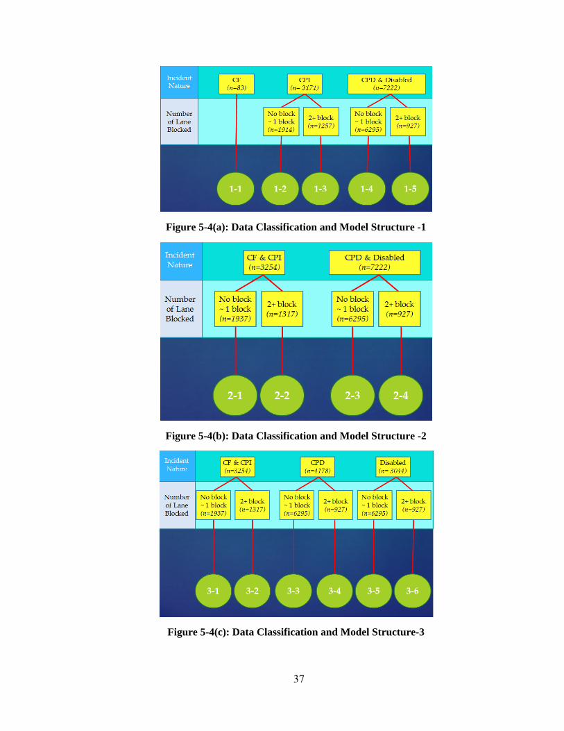
37

Figure 5-4(a): Data Classification and Model Structure -1

Figure 5-4(b): Data Classification and Model Structure -2

Figure 5-4(c): Data Classification and Model Structure-3

38

Estimation results

Note that two different ordering sequences for variables were used to calibrate the BN

model parameters. The first one (Ordering -1) is: Road > Operation Center > Time > Pavement

Condition > Total Number of Vehicles > Lane Closure > Incident Nature > Heavy Vehicles >

Duration. In this ordering sequence, Duration has the lowest rank to be a parent of all other

variables.

The second ordering sequence (Ordering-2) was based on the knowledge of field

operators, as follows: Incident Nature > Total Number of Vehicles > Lane Closure > Pavement

Condition > Time > Road > Operation Center > Heavy Vehicles > Duration. The estimation

results of each data group using the K2-algorithm under these two order sequences and their BIC

scores are presented in the remaining section.

Table 5-2: BIC Scores of Different Models

Model BIC Scores

Full Model – Ordering 1 -1809.832

Full Model – Ordering 2 -2403.019

Serious Model – Ordering 1 -680.9486

Serious Model – Ordering 2 -564.1333

Non-Serious Model – Ordering 1 -953.27023

Non-Serious Model – Ordering 2 -752.94533

Table 5-2 shows the BIS score for each model, where the full model under Ordering-1

yields a better performance than under Ordering-2. However, the partial-information models,

comprising Serious/Non-Serious injury categories, achieve a better accuracy under the Ordering-

2 sequence. Hence, Ordering-1 was used to build the Full model and Ordering-2 was applied to

construct the partial-information models.

Table 5-3 lists all variables used for developing both the full and the partial-information

models (i.e., incidents resulting in serious and non-serious injuries). The Non-Serious submodel

in the latter was developed with incident data of disabled vehicles and collision/property damage,

while the Serious model used injury and fatality incident data for parameter calibration.

39

The prediction result with the full model is shown in Table 5-4, where most predicted

clearance durations fall into two categories: the 1-15 minutes and 30-more minutes. The

accuracy rate of the15-30 minutes category is much lower than other two categories. Overall, it

reflects the fact that the data quality cannot support the models to perform the prediction of

incident clearance duration at the precision level of 15 minutes. The overall accuracy rate of the

full model is 54 percent if one divides all incident clearance durations at the range of 15-minutes

intervals. However, by classifying incident clearance durations into two categories of either less

or over 30 minutes, the full model yields an acceptable level of prediction results, as shown in

Table 5-5, where the model can correctly predict the duration for about 90 percent of less-severe

incidents.

Table 5-3: List of Variables used in the Full Models and Serious/Non-Serious Models

Variable Full Models Serious/Non-Serious

Models

Clearance Time 1-918 minutes Same

Incident Nature

(1) Collision and Fatality, (2) Collision and Injury,

(3) Collision and Property Damage, (4) Disabled

Vehicle

N/A

Pavement Condition Snow, Dry, Wet, and Chemical Wet Same

Time

(1) Weekday Off-peak, (2) Weekday Peak,

(3) Weekday Night, (4) Weekend Day,

(5) Weekend Night

Same

No. Vehicles One, Two, Three and Four or More One or Two and Three or

more

No. Heavy Vehicles Zero, One and Two or More Yes/No

Lane Closure

(1) No Block, (2) Shoulder Block, (3) One-Lane

Block, (4) Two-Lane Block, (5) Three-Lane

Block, (6) Four or More Lane Block

No or shoulder, One or

two and More than three

Operation Center AOC, SOC, TOC3, TOC4 and TOC7 Same

Road I-70, I-95, I-270,I-495, I-695 and US-50 Same

40

The prediction results with the Serious/Non-Serious injury model are shown in Table 5-6

and Table 5-7. Note that the Serious-injury model was designed to explore the potential of

predicting the clearance duration of serious-injury incidents at the precision level of 20 minutes.

It, however, yields only an accuracy rate of 44 percent. A more ambitious attempt with the Non-

Serious model was to predict the clearance duration of an incident at the precision level of eight

minutes, but the estimation results in Table 5-7 indicate that both the data quality and model

performance cannot support traffic managers’ expectation of having such information at this high

precision level.

In addition to using the correctly predicted percentage for evaluation, Table 5-7 also

shows the comparison results with three performance indicators, where the full-information

model with the interval of 30 minutes outperforms all other prediction models.

Table 5-4: Full model prediction results with three categories of incident clearance durations

Category Predicted

Actual

1-15 minutes 15-30 minutes 30+ minutes Accuracy 1-15 minutes 921 51 202 78% 15-30 minutes 397 131 260 17% 30+ minutes 278 75 601 63%

Table 5-5: Full model prediction results with two categories of incident duration

Category Predicted

Actual 1-30 minutes More than 30 minutes Accuracy

1-30 minutes 1722 250 87% More than 30 minutes 606 337 36%

Table 5-6: Serious-injury model prediction results

Predicted

Actual

1-20 minutes 20-40 minutes 40+ minutes Accuracy 1-20 minutes 115 35 107 45% 20-40 minutes 105 57 107 21% 40+ minutes 71 46 194 62%

41

Table 5-7: Non-serious model prediction results

Predicted

Actual

1-8 minutes 8-15 minutes 15-30 minutes 30+ minutes Accuracy1-8 minutes 285 139 124 2 52% 8-15 minutes 193 210 124 5 39% 15-30 minutes 138 205 158 6 31% 30+ minutes 236 147 99 9 2%

Table 5-8: Non-serious model prediction results

Full Model Serious Model Non-Serious Model

Logarithmic loss 1.002 1.055 1.348

Quadratic loss 0.597 0.6377 0.7318

Spherical payoff 0.633 0.6015 0.5175

Note that the above models’ undesirable performance can be attributed partly to the

incomplete collision information collected by CHART, which only classifies all collision-

incidents into five categories: disabled vehicles, collision and property damage, collision and

injury, and collision and fatality. Some critical data, such as the number of injuries or fatalities,

are not recorded in the CHART’s database. In contrast, the database in MAARS contains more

detailed information on each collision-incident, which includes: disabled vehicle, fatality,

property damage, incapacitating injuries, possible incapacitating injuries, and non-incapacitating

injuries. However, MAARS does not record traffic condition and lane-blockage data during

incident clearance operations. Hence, to cope with the data deficiencies, one alternative is to

merge the CHART and MAARS database into a new synthesized database that contains mutually

supplemental information for better model calibration.

Table 5-9 shows the incident classification in the CHART and MAARS databases.

Because these two databases use different formats to record their own concerned data, it is

difficult to identify the same incident and to merge all associated data from these two systems.

Table 5-10 presents two sets of criteria used in matching those incidents recorded by both

databases: the incident reported date, time, located county, route name, incident nature, or

number of involved vehicles. Note that due to both the data recording quality and the format

42

discrepancy, the number of correctly matched cases decreases with the number of criteria used

for identifying incidents.

Table 5-9: Incident Classification in the CHART and MAARS Databases

CHART MAARS

Categories

(1) Collision and Fatality

(2) Collision and Injury

(3) Collision and Property Damage

(4) Disabled Vehicle

(1) Collision and Fatality

(2) Collision and Incapacitating Injury

(3) Collision and Possible Incapacitating

Injury

(4) Collision and Non Incapacitating

Injury

(5) Collision and Property Damage

(6) Disabled Vehicle

Table 5-10: Criteria used in merging incident data from the CHART and MAARS Databases

Criteria Description

Level-1

1. Time difference within twenty minutes on the same day

2. Same county

3. Same Route

4. Difference in the number of vehicles involved does not exceed one vehicle

Level-2

1. Time difference within twenty minutes on the same day

2. Same county

3. Same Route

4. Same Incident Nature as classified in Table 4-9.

Using the correctly merged dataset to recalibrate the full model at an interval of 15

minutes and 30 minutes, the prediction results, as expected, are better than those based only on

the collision information from CHART. For example, the full model calibrated with the merged

dataset can improve its prediction accuracy for incidents between 1-15 minutes from 78 percent

to 84 percent, and for those over 30 minutes from 36 percent to 46 percent (see Table 5-11) if

viewing the interval of 15 minutes as an acceptable variance range. Similarly, if the main

43

concern on a detected incident is whether or not its clearance duration will exceed 30 minutes,

the full model calibrated with the merged dataset can improve its prediction accuracy for short-

duration incidents (i.e., less than 30 minutes) from 87 percent to 97 percent.

Table 5-11: Prediction results by the full model based on the merged dataset

Predicted

Actual

1-15 minutes 15-30 minutes 30+ minutes Accuracy

1-15 minutes 858 7 154 84%

15-30 minutes 364 21 191 4%

30+ minutes 333 16 292 46%

Table 5-12: Full model prediction results based on the interval of 30 minutes

Predicted

Actual

1-30 minutes More than 30 minutes Accuracy

1-30 minutes 1562 53 97%

More than 30 minutes 549 73 12%

Note that the above prediction results reflect the common deficiency of all developed

models in predicting the clearance duration of more severe incidents lasting more than 30

minutes. This is likely due to two reasons: (1) the clearance durations of more than 65 percent of

incidents recorded in both the CHART and MAARS databases are less than 30 minutes,

naturally causing a bias in model calibration and prediction; and (2) incidents lasting longer time

periods generally attribute to many complex factors that are not all recorded in these two

databases.

Classified by incident nature and lane-blockage information

To contend with the difficulty of predicting the clearance duration of severe incidents, the

research team also explored the alternative of developing a model for each incident group

classified sequentially by incident nature and the number of blocked lanes. The performance of

each prediction model under different incident intervals is shown in Figure 5-5.

44

The first set of prediction results presented in Figure 5-5(a) includes the following

incident clearance models: collision/fatality(CF), collision/property damage/injury (CPI)-one or

no blocked lane, collision/property damage/injury(CPI)-two or more blocked lanes,

collision/property damage/disabled vehicle (CPI-disabled)-one or no blocked lane, and

collision/property damage/disabled vehicle (CPI-disabled)-two or more blocked lanes. The

prediction results reveal a consistent pattern across all models, that is, those short-duration but

high frequency incidents are likely to be predicted correctly. For those incidents lasting over 40

minutes, only the model for the category of collision/property damage/disabled vehicle(CPD-

disabled)-two or more blocked lanes produces an acceptable accuracy (72 percent) even at the

precision of 20 minutes.

The second set of performance results, shown in Figure 5-5(b), includes the combined

CF&CPI models and the CPD-disabled models under two types of lane-blockage conditions. The

former set of models calibrated with severe incident data yields somewhat promising results,

where the one for incidents causing no or one blocked lane can achieve 94 percent and 82

percent accuracy for those under 20 minutes and between 20-60 minutes, respectively. In

contrast, for incidents in the same duration categories but blocking multiple lanes, the model for

CF&CPI- two or more blocked lanes can correctly predict only 71 percent and 57 percent,

respectively, out of all sample cases. Both sets of models cannot yield acceptable prediction

results for those incidents lasting over 60 minutes, reflecting that some additional factors that

complicate the clearance operations may not be recorded in the database.

The last step of this model analysis is to first separate those incidents classified as CPD

and disabled-vehicles into two groups, and then further divide them into two subgroups based on

the resulting number of blocked lanes. The performance results are shown in Table 5-5(c), where

both CPD models show sufficiently reliable capability for predicting all incidents lasting less

than 60 minutes. The models for disabled-vehicles, due apparently to its sample distribution,

yield perfect prediction for those lasting less than 15 minutes, but not for the remaining incidents

in the same category.

45

Figure 5-5(a) Estimation results of clearance time prediction models

Figure 5-5(b) Estimation results of clearance time prediction models

46

Figure 5-5(c) Estimation results of clearance time prediction models

5.5 Conclusion

Recognizing the critical role of incident clearance duration in design of traffic

management strategies, this chapter presents an advanced Bayesian network method for model

development using both the CHART and MAARS datasets. Due to the complex impacts of

various factors on incident clearance operations and the quality of the available data, some

developed models are not capable of producing a desirable level of accuracy. While much

remains to be learned about critical factors influencing incident clearance operations, some

suggestions for future development are listed below:

• All factors affecting incident clearance duration need to be precisely collected and

recorded in the database.

• Neither CHART nor MAARS records all critical factors affecting the incident clearance

operations, so some efforts to merge these two mutually supplemental data systems will

be an essential task.

47

• Both datasets should have a reliable quality control mechanism to filter faulty data and

identify the data precision level (e.g., 5 minutes). The large number of short duration data

(e.g., less than 2 minutes) that heavily bias the sample distribution makes model

development an extremely difficult task.

• Data recording efforts should be improved as both datasets contain a large percentage of

missing data (e.g., number of blocked lanes) for each recorded incident.

• One model for all types of incidents is unlikely to be effective due to the variety of

factors that may affect the progress of an incident management team.

• Classifying incident data by the severity level and the resulting blocked lanes seems to be

a promising way to develop a comprehensive set of prediction models for incident

clearance duration.

48

CHAPTER 6: Optimal Strategies for Deploying Freeway Incident Response Units

6.1 Introduction

This chapter presents an optimization strategy for SHA to effectively distribute incident

response units along freeway segments plagued by frequent incidents. The proposed method,

based on the p-median model, convincingly outperforms three state-of-practice deployment

strategies, using the incident data from 2006 to 2011 on the I-495 Capital Beltway. Section 6.2

reviews the available strategies for deploying emergency response units and relative studies in

the literature. Section 6-3 analyzes the formulations of several promising deployment models,

including the one developed from this project. Section 5-4 illustrates a comprehensive

benefit/cost analysis with different response fleet sizes. Research findings produced from

extensive analyses of the developed model are summarized in the last section, providing a basis

for traffic managers to design a benefit-cost incident management system.

6.2 Review of available models

Traffic incident is a major cause of roadway congestion and the related adverse

environmental impacts. For example, Skabardonis et al. (2003) found that incident-related delay

contributed from 13 to 30 percent of the total congestion delay during peak periods, based on an

analysis of two freeway corridors in California. In a more comprehensive study, FHWA (2005)

found that about 25 percent of congestion in the US is incident-related, indicating the need to

have an effective incident management system that includes detection, response, and traffic

management to contend with non-recurrent congestion. For instance, prompt responses by

CHART have reduced the incident durations by about 25 percent for the last seven years (Chang,

2009), yielding significant benefits to both motorists and the entire travel environment.

Since efficient response is critical to minimization of incident impacts, many traffic

management agencies are exploring various strategies to best use their limited emergency

response units. For example, some (Skabardonis, 1998; Lou, 2010) introduced a freeway service

patrols (FSP) program to assign tow trucks to patrol freeway segments and clear incidents. In

highway networks where traffic surveillance and incident detection are available, some

researchers (Larson and Odoni, 1981; Pal and Bose, 2009) argued that it is more efficient to

49

deploy response units strategically and dispatch them after detecting an incident. The key

question for designing such strategies is how to deploy available response units to minimize the

response time.

In practice, most traffic managers tend to use experience-based methods such as

allocating available response units near high-frequency incident locations, distributing them

evenly over the entire coverage area, or positioning standing-by units at the Traffic Operation

Center (TOC). Such experience-based methods, however, may not best use available resources,

especially when the incident frequency or coverage area is not at the desirable level. This study

has produced an effective method for deploying emergency response units, taking advantage of

state-of-the-art developments in the literature.

Most existing studies related to this subject can be categorized into two categories:

median and coverage models. The former, first introduced by Hakimi (1964) in the context of

deciding facility locations, seeks to position emergency units to minimize the average response

distance or time. Following the same modeling paradigm, Daskin (1987) constructed a mixed-

integer programming (MIP) model to solve the location, dispatching, and routing problems for

incident response vehicles. Pal and Sinha (1997) introduced a similar model to determine the

optimal locations for incident response units to minimize the total operating cost.

In contrast, coverage models focus on minimizing the number of response units required

to cover the target area with a predefined level of service (Toregas, 1971), or maximizing the

demand that can be covered by the available emergency units, known as the Maximal Coverage

Location Problem (MCLP) introduced by Church and Revelle (1974). As an extension to MCLP,

Daskin and Stern (1981) proposed the Backup Coverage Problem to maximize the demand areas

to be covered multiple times, while Gendreau et al. (1997) considered two different service

standards for coverage. Kepaptsoglou et al. (2011) applied Genetic Algorithm to solve a DSM of

emergency response services considering historical frequency and severity as the primary

standards. It does not, however, account for variation in travel time.

A main criticism of these models is their common assumption that the closest response

unit is always available. Mirchandani and Odoni (1979) observed that the policy of dispatching

the closest response unit is not always optimal when the response units have a high probability of

being occupied. The Hypercube Queuing Model (HQM) developed by Larson (1974) proves to

be a very useful tool to evaluate the performance of emergency response systems while

50

considering the stochastic nature of incidents. However, HQM requires the locations of response

units to be input and cannot determine the optimal configuration of the system (2009).

To address the same stochastic issue in such a system, Daskin and Haghani (1984)

proposed a heuristic approach to minimize the expected arrival time. Sherali and Subramanian

(1999) introduced an opportunity-cost-based model to consider the loss of coverage when one

unit becomes occupied. Geroliminis et al. (2009) extended HQM to build a normative model that

can generate optimal strategies, while considering spatial and temporal patterns of the demand

and the availability of a response unit. Their paper presented two key findings: (1) the MCLP

model does not perform well when considering the stochastic nature and availability of the

response units; and (2) the traditional p-median model can provide an “adequate approximation”

to the results by the more complex models, adding only 4 percent of average response time for

the modest demand (i.e., one incident/hour on a 72 mile freeway segment).

Another concern associated with existing models is their deficiencies in modeling the

impact of future demand uncertainty. Since incident patterns may evolve significantly over time,

an emergency response system designed with the historical data may not always perform well

under the changing traffic environments. This critical issue of adapting to the temporal and

spatial changes in incident patterns with a robust deployment strategy has not been adequately

addressed yet in the literature.

One critical issue in designing a deployment strategy is to maximize the resulting social

benefits and minimize operating costs, because most traffic management agencies are operated

under resource constraints. Hence, the challenge is how to deploy the available EMS units to

maximize the total social benefits, or to identify the optimal number of EMS under the projected

incident distribution pattern. A comprehensive cost/benefit analysis of various location/allocation

strategies under a projected incident pattern could help traffic agencies to optimize their fleet

size.

To address the above concerns, this study presents a two-stage process to model the task

of deploying emergency response units. It first compares the performance of the optimal

incident response strategy based on the p-median model with three experience-based methods.

The comparison was based on the incident data from 2006 to 2011 on the I-495 Capital Beltway,

using different fleet sizes and their resulting costs as well as benefits.

51

6.3 Model Formulation

This section investigates three experience-based methods for allocating emergence

response units, including 1) allocating available response units near high-frequency incident

locations, 2) distributing them evenly over the entire coverage area, and 3) positioning standing-

by units at the Traffic Operation Center (TOC).

Consider I regions to be served by no more than P emergency response units over J

potential sites; M ( is the set of location sites to house the response units. In general, given

the following inputs:

• , travel cost from location j to region i; and

• , the probability that an accident occurs in service region i during a given time

period,

The allocation model to minimize the total response time should yield the following output:

• a response strategy Y as follows:

(6-1)

• an allocation strategy, denoted by X, where each member xij equals 1, if accidents at

region i are to be managed by the response units located at location j, and 0 otherwise.

The spatial distribution of accidents is represented by . Traffic management

agencies can formulate their strategies, X and Y, based on the historical data.

After classifying the accident pattern, traffic agencies can then evaluate the selected

candidate strategies based on the following annual total response time:

(6-2) where for the n-th incident of the year,

(6-3)

In addition, given the selected allocation strategy, it may also be desirable for the traffic

agencies to further decide the most cost-benefit number of response units, P. This issue will be

addressed in the next section.

52

Experience-based strategies

Strategy-I

Under this strategy all emergency response units will be stationed at the P sites that

exhibit high incident rates, and the strategies Y and al X can then be decided as follows:

Step1: Choose the P sites with the highest incident rates to form the location site M. If several

sites have the same incident rates, then randomly choose P sites from them. Assign

proper values to Y according to Equation 1.

Step2: For each site , find the closest site among all candidate locations that satisfy

and assign response unit at for any incident at by:

(6-4)

Although previous studies suggested that dispatching the closest response unit to a

detected incident does not necessarily guarantee the best result, such a strategy is simple and thus

widely practiced. Assuming that only one incident may occur within a small segment over a

sliced time interval, the response strategy can then be uniquely determined by following steps 1

and 2. The annual response time, based on the historical data, can be calculated with Equation 2

for comparison with other strategies. This strategy can generally reduce the response time at the

historical “hot spots” in the service area. However, if these locations are overly concentrated at

one corner of the service area, the strategy may not perform well, especially when those “hot

spots” may vary over time.

Strategy-II

The second experience-based strategy seeks to distribute emergency response units

evenly over the entire coverage area so that no location would suffer excessively long incident

response time. This problem can be formulated as:

min = (6-5) . . = 1 ∈ ∈ (6-6)

53

where dij represents the travel distance between the response unit j and the service request

location i. Equation 6 guarantees that one and only one response unit will be assigned to each

site. This problem has been proved as NP-hard in the literature. Moreover, it does not consider

the differences of accident frequency and travel time at different locations. Therefore, this study

will not further discuss its algorithm for an exact solution. Instead, the numerical example

provided in this study will take advantage of the unique structure of the Beltway and solve the

problem heuristically by the following steps:

Step 1: Divide the Beltway into P segments with equal length .

Step 2: Choose the site closest to the center of each segment to form the location site M.

Step 3: Assign response units to these locations and decide Y according to Equation 1.

Step 4: For each site , find the segment it belongs and the center location for this segment,

then assign response unit at for site by following Equation 4.

Strategy-III

In practice, traffic management agencies could also position standing-by units at their

traffic operation center (TOC). One can illustrate their response strategy as follows:

Step1:

(6-7)

Step2: If the response agency has one TOC (as in the numerical example), then

(6-8)

If multiple TOC are available, then one needs to find the closest one for each site. The response

time can then be uniquely determined from all regions I to the region where the TOC locates.

Strategies based on the proposed p-median model

Following the same arguments by Geroliminis et al. (2009), this study developed an

optimal incident response strategy based on the traditional p-median model, which is both

effective and convenient for implementation. The underlying assumption for this method is that

54

the occurrence of incidents on a given freeway segment follows a Poisson distribution, and the

probability for more than two accidents occurring during the same sliced time period on the same

segment is negligible (i.e., an average of 0.2 on I-495 Capital Beltway). Following previous

studies in the literature, the objective function of a traffic management agency can be formulated

as follows:

(6-9)

where: tij represents the travel cost from location j to freeway segment i. For convenience of

illustration, this model does not consider intra-zonal times (assume tii =0), and uses the average

travel time based on field data. The model can be further extended to consider speed variation

and uncertainties in the future work.

Note that both the demand and the supply sides are subjected to the following constraints:

1) every freeway segment i must be served; 2) a response unit can only be dispatched from

location j if it is available (yj=1); and 3) the total number of available response units is limited by

available resources (P). Constraint 1 can be expressed as:

(6-10)

Constraint 2 is formulated as:

(6-11)

By introducing a large number L (which should be equal to or larger than I), constraint 2 can be

re-formulated as:

(6-12)

Similarly, constraint 3 can simply be expressed as:

(6-13)

Given the formulations, the allocation task for incident response units becomes a p-

55

median problem with the following two binary sets of decision variables:

One can then apply the model to decide the optimal locations for available incident

response vehicles, given the empirical distribution of accidents on each freeway segment and the

corresponding travel cost matrix.

6.4 Numerical results

Note that the numerical results for I-495 Capital Beltway presented hereafter were

produced with GAMS, a commercial optimization software package. The annual response time

and the associated costs and benefits were also computed for comparison with other experience-

based strategies.

Study Site

The study site is the Capital Beltway (I-495/I-95) in Maryland, ranging from the DC-VA

state Line at the Woodrow Wilson Bridge to the VA Line at the American Legion Bridge (see

Figure 5-1). The Beltway has 30 exits distributed over 42 miles, one of the major corridors

managed by CHART.

56

Figure 6-1: Study Links in the Capital Beltway (I-495/I-95) in Maryland

TOC-3 (Traffic Operation Center-3) of CHART, currently located at exit 25, has 11 field

operations units to manage incidents on I-95, I-270, US-50, MD-295 as well as the Capital

Beltway in Prince George’s and Montgomery Counties. They operate over 16 hours/day (5 AM –

9 PM) on weekdays.

The proposed model was applied to determine the optimized locations for their EMS

units over the Capital Beltway to minimize the total and average incidents response times during

AM peak hours (7:00 – 9:30) on weekdays. Travel speeds on each freeway segment were

collected from the freeway detectors documented by CATT (the Center for Advanced

Transportation Technology) laboratory at the University of Maryland.

T

57

Figure 6-2: Average Traffic Speed Patterns for the AM Peak Hours by Day of Week

(I-495 Outer Loop)

Figure 6-3: Average Traffic Speed Patterns for the AM Peak Hours by Day of Week

(I-495 Inner Loop)

Traffic

Traffic

58

Figures 6-2 and 6-3 summarize the average speed during the morning peak period for

different days of the week in 2009. The figures indicate that the average traffic speeds on most

segments exhibited very similar patterns over different weekdays and for both directions. Only

segments from exit 27 to exit 31 (about 5 miles) in the Outer Loop exhibited a significant

fluctuation. Since it is a small portion of the entire network, this study will not consider travel

time variation as one of the model variables.

The results in Figures 6-2 and 6-3 show very different traffic conditions in the opposite

directions. Therefore, travel times (response times) for response units would vary significantly,

depending on the travel direction. Thus, travel time data used in this study are asymmetric. The

average morning peak travel time on each highway segment in 2010 was used in the numerical

analysis.

Data

This study used the incident data from CHART II Database to evaluate the performance

of different strategies. CHART database includes eight incident types:

1. Debris in Roadway 2. Collision, Personal Injury 3. Collision, Property Damage 4. Collision, Fatality 5. Disabled on Road 6. Emergency Roadwork 7. Police Activity 8. Off Road Activity

Notably, incidents with a different nature and severity could result in different traffic

impacts. Prior to having the incident severity information from field observations, CHART

views all detected incidents equally and responds to them sequentially. However, if incident

severity has been verified, CHART will give the response priority to more severe incidents.

Since the focus of this model is to minimize the response time but not the clearance time, the

numerical results, presented below with the response allocation models, were based only on the

spatial distribution of incident frequency.

For convenience of analysis, both the demand (incidents) and supply (response units) are

assumed to be located at the nodes (i.e., freeway exits) of each link, and the travel times between

nodes were calculated based on the procedure described previously. Incident data from 2006 to

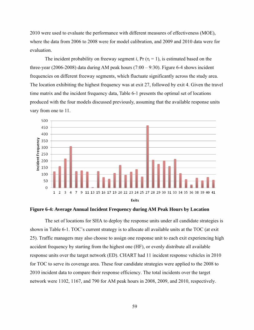
59

2010 were used to evaluate the performance with different measures of effectiveness (MOE),

where the data from 2006 to 2008 were for model calibration, and 2009 and 2010 data were for

evaluation.

The incident probability on freeway segment i, Pr (τi = 1), is estimated based on the

three-year (2006-2008) data during AM peak hours (7:00 – 9:30). Figure 6-4 shows incident

frequencies on different freeway segments, which fluctuate significantly across the study area.

The location exhibiting the highest frequency was at exit 27, followed by exit 4. Given the travel

time matrix and the incident frequency data, Table 6-1 presents the optimal set of locations

produced with the four models discussed previously, assuming that the available response units

vary from one to 11.

Figure 6-4: Average Annual Incident Frequency during AM Peak Hours by Location

The set of locations for SHA to deploy the response units under all candidate strategies is

shown in Table 6-1. TOC’s current strategy is to allocate all available units at the TOC (at exit

25). Traffic managers may also choose to assign one response unit to each exit experiencing high

accident frequency by starting from the highest one (HF), or evenly distribute all available

response units over the target network (ED). CHART had 11 incident response vehicles in 2010

for TOC to serve its coverage area. These four candidate strategies were applied to the 2008 to

2010 incident data to compare their response efficiency. The total incidents over the target

network were 1102, 1167, and 790 for AM peak hours in 2008, 2009, and 2010, respectively.

60

Table 6-1: Assigned Locations for Available Response Units by Strategy

No. of Units

Available

Assigned Exit(s) by

OPT* TOC HF ED

1 23 25 27 22

2 7, 30 N/A 4, 27 11, 31

3 4, 22, 33 N/A 3, 4, 27 7, 22, 34

4 4, 20, 29, 35 N/A 3, 4, 27, 33 4, 16, 27, 36

5 4, 17, 25, 30, 35 N/A 3, 4, 27, 28, 33 4, 13, 22, 29, 38

6 3, 9, 19, 25, 30, 35 N/A 3, 4, 27, 28, 30, 33 4, 11, 19, 24, 31,

38

7 3, 9, 19, 25, 30, 34,

40 N/A

3, 4, 27, 28, 29,

30, 33

3, 9, 15, 22, 27,

33, 38

8 3, 9, 16, 20, 25, 30,

34, 40 N/A

3, 4, 20, 27, 28,

29, 30, 33

3, 9, 13, 19, 24,

28, 33, 39

9 3, 9, 16, 20, 23, 27,

30, 34, 40 N/A

2, 3, 4, 20, 27, 28,

29, 30, 33

3, 7, 11, 17, 22,

25, 30, 34, 39

10 2, 4, 9, 16, 20, 23,

27, 30, 34, 40 N/A

2, 3, 4, 20, 27, 28,

29, 30, 31, 33

3, 7, 11, 15, 19,

23, 28, 31, 34, 39

11 2, 4, 9, 16, 20, 23,

27, 28, 30, 34, 40 N/A

2, 3, 4, 20, 24, 27,

28, 29, 30, 31, 33

3, 7, 9, 13, 17, 22,

25, 28, 31, 35, 39

*OPT: the proposed model; HF: to the top N (= available units) high incident-frequency locations; TOC: stationed all vehicles at the traffic operations center; ED: evenly distributed.

61

* Note that the total travel time under the TOC strategy was constant irrespective of the available fleet size

Figure 6-5: Total Travel Times (in minutes) by Incident Response Strategy

Year

Year Year

62

Figure 6-5 illustrates the estimated total travel time (response times) by allocating

response units according to each strategy. Note that the total travel time under the TOC strategy

was constant irrespective of the available fleet size, and hence only its results from the first

scenario were shown in the figure.

As shown in the graphical results, the proposed model consistently outperforms other

strategies in most cases across all three years. The only exception is for the single unit case

where the system randomness can dictate the performance. For instance, for the response unit

size of five, the estimated total travel times by OPT, HF, and ED are 2194, 3302, 2630 minutes,

respectively, for year 2009. These differences imply that the total travel time with the OPT

strategy would be reduced by about 34 percent and 17 percent compared with HF and ED,

respectively. The response time savings are also significant for 2008 and 2010. Overall, the

percentage improvement increases with the number of available response units and the incident

frequency.

Note that given the small chance of concurrently detecting several incidents on the same

subsgement of the I495 Capital Beltway, SHA can maintain a small size of response teams by

positioning all standing-by units at the TOC center. The trade-off to the cost savings, however,

could be a long response time if an incident happens at a remote location. Given the huge cost of

having an extended delay on congested freeways such as the I-495 Capital Beltway, this strategy

is unlikely to outperform any other strategies.

The optimal fleet size from the Cost-Benefit Perspective

Note that the above analysis provides the optimal deployment strategy for the available

EMS units. However, in view of the societal cost and the diminishing resources for traffic

management, one shall further explore the optimal number of EMS under the projected

distribution of incidents and traffic patterns. The total societal cost reduction due to an efficient

incident response strategy includes the savings on incident-induced delay, fuel consumption, and

emissions.

Various formulas have been proposed in the literature to estimate delays and the

associated benefits. To be consistent with the practice of SHA and take advantage of the locally

calibrated parameters, this research adopts the following procedure for total delay and direct

benefit estimation (Chang, 2009):

63

(6-14)

where:

D is total excessive delay incurred by the incidents on top of the recurrent congestion;

f is traffic volume (vplph) at the segment i;

b and n are the number of lanes blocked and the total number of lanes, respectively;

d is the average incident duration (hours) at the segment i;

N is the total number of incidents at the segment i; and μ, φ, θ, and γ are parameters. This study used -10.19, 2.8, 1.4, and 1.78, respectively, as

recommended by CHART.

Table 6-2 shows the additional information required to estimate total delay caused by

incidents occurring during the morning peak hours in 2008 through 2010. Due to the lack of

traffic volume during each incident period this study used the adjusted Average Annual Daily

Traffic (AADT) volume as a proxy factor. The incident duration is defined as the sum of

response time and clearance time, where the latter was obtained directly from the CHART

database and the former was computed with the proposed optimal model.

Table 6-2: Traffic and Incident Information Used to Estimate Incident-Induced Delays

Variables 2008 2009 2010

AADT on I-495 189,383 195,238 195,171

PHF 0.95 0.95 0.95

Adjusted AADT for Peak Hours 199,350 205,513 205,443

Number of Lanes (one direction) 4 4 4

Average Clearance Time with CHART Response

(minutes) 26.30 23.85 16.74

Average Lane Blockage due to Incidents 1 1 1

Using Equation 6-13 and information in Table 6-2, the total delays caused by incidents,

assumed to be responded to by each candidate strategy, are summarized in Figure 6-6. Similar to

the results in Figure 6-5, the developed strategy (OPT) clearly outperforms other strategies in

most scenarios. For example, with a unit size of 10, the total delays estimated for year 2009 are

64

403587, 436149, and 416252 vehicle-hours for OPT, HF, and ED, respectively. The proposed

strategy, OPT, reduces the total delay by about 55 percent and 13 percent compared with HF and

ED, respectively.

Figure 6-6: Total Delays (in vehicle-hour) for Incident Responses by Strategy

Year

Year

Year

65

Based on the computed total delay, one can estimate the resulting cost savings with the

following procedures:

Step 1: Compute the total delay reduction with each candidate strategy.

Step 2: Estimate the fuel consumption and emissions from the delay reduction using

the following information.

• Fuel consumption for passenger cars: 0.156 gallons of gasoline / hour of delay (Ohio Air

Quality Development Authority)

• HC: 13.073 grams / hour of delay (provided by MDOT in 2000)

• CO: 146.831 grams / hour of delay (provided by MDOT in 2000)

• NO: 6.261 grams / hour of delay (provided by MDOT in 2000)

• CO2: 19.56 lbs CO2 / gallon of gasoline (Energy Information Administration)

Step 3: Convert the saved delay, fuel, and emissions to the monetary value

Similar to Step 3, these following conversion factors were used to estimate the reduced

delay and associated by-products in the total monetary value:

• Delay: $26.58/ hour (U.S. Census Bureau in 2006)

• Fuel: $3.85/gallon (Apr.- Sep.) , 2.72/gallon(Energy Information Administration in 2008)

$2.32/gallon (Energy Information Administration in 2009)

• HC: $6,700/ton (DeCorla-Souza, 1998)

• CO: $6,360/ton (DeCorla-Souza, 1998)

• NO: $12,875/ton (DeCorla-Souza, 1998)

• CO2: $23 / metric ton (CBO (Congressional Budget Office)’s cost estimate for S. 2191,

America’s Climate Security Act of 2007)

To analyze how the additional response units would contribute to the system’s efficiency,

this study has evaluated the marginal benefit/cost for adding another unit to the EMS team,

ranging from 1 to 11 units, given the estimated marginal cost by SHA. Based on the results

shown in Figure 6-7, the marginal benefit/cost first decreases as the number of response units

increase, but the pattern becomes relatively flat if deploying more than 7 units. Therefore, the

benefits of adding additional response units become insignificant when the size of the response

fleet is larger than 7, although the B/C ratio could still be greater than 1. The pattern is consistent

over the three-year period, although the magnitude of B/C ratio fluctuates from year to year. The

66

information produced by this analysis can serve as the basis for CHART to decide the most cost-

beneficial fleet size.

Figure 6-7: Marginal Benefit-Cost Ratios for adding an Additional Response Unit

67

CHAPTER 7: Conclusions

7.1 Conclusions

This study was focused on identifying potential areas for CHART to enhance its

operations efficiency and to maximize the resulting benefits under existing resource constraints.

Its core tasks cover three imperative issues: (1) understanding critical factors contributing to an

increase in incident response and clearance times; (2) designing a deployment strategy to

optimally assign available highway patrol units to minimize incident response times based on the

temporal and spatial distributions of historical incidents; and (3) developing reliable models to

predict the required duration of a detected incident and to identify critical contributing factors.

Some critical research findings summarized below could be informative for CHART to

effectively redesign and improve its incident response strategies:

• Using the incident data from 2006 to 2011 on the I-495 Capital Beltway, this research has

shown the potential for CHART to significantly reduce its response efficiency and to

determine the optimal fleet size by using an optimal vehicle assignment model.

• The incident data collected by CHART can be integrated with information in MAARS to

develop a reliable model to predict the required clearance duration of a detected incident.

Such vital data can serve as the basis for estimating the range of incident impact and

designing responsive traveler information systems.

• CHART’s response efficiency is not consistent, varying with factors such as incident

severity, traffic congestion, weather conditions, fatalities, and pavement conditions. For

example, the average response time for property-damage only incidents is longer than for

those with injuries and/or fatalities.

• All CHART’s response centers consistently took shorter times to respond to incidents

resulting in more traffic impacts such as causing multiple lane blockage or fatalities.

• The average response times among CHART’s five operations centers differ significantly:

TOC7 exhibited the longest average of around 9.5 minutes and AOC had the shortest

time of 4.5 minutes from 2007-2009.

• The distribution of available resources (e.g., tow trucks and staff size) among CHART’s

five operations centers significantly affects the efficiency of their response.

68

• The resulting clearance time of a detected incident depends on various factors, including:

incident nature and severity, the need and availability of any special equipment, the

coordination between all responsible agencies (e.g., police, fire department, medical

team), and incident location.

• Truck involvement, multi-lane closure, and fatalities are three critical factors contributing

to most excessively long incident clearance times.

• Most incidents (83 percent) involving fatalities took more than two hours to recover the

roadway traffic condition, revealing the need for better coordination with responsible

medical agencies.

• The efficiency of incident clearance of CHART’s five response centers varies with the

weather and environmental conditions; i.e., the average clearance duration at night time

and/or a snow condition is substantially longer than the duration under day time and

normal weather environments.

• The discrepancies in the average incident clearance time among CHART’s five response

centers reflect not only the difference in each center’s responded incident types and

frequency, but also in the distribution of the required equipment/vehicles and staff to

accomplish the mission.

In summary, using the information from CHART and MAARS, this research has

identified critical factors affecting the CHART’s efficiency in incident response and clearance

and produced reliable models to improve its performance in incident traffic management. The

optimal allocation model will enable each operational center to best deploy available patrol

vehicles along its responsible highway networks and to select the most cost-benefit fleet size

under the resource constraints. CHART can also apply the set of prediction models developed in

this research to estimate the required clearance duration of a detected incident, thereby

minimizing the resulting congestion within the impact boundaries via some real-time traffic

control strategies. Incorporating any of those developed models into current practice will

undoubtedly enhance CHART’s operational quality and significantly increase its effectiveness in

minimizing non-recurrent congestion in this region.

69

7.2 Recommendations

Despite the progress made in this research on improving incident response and clearance

operations, much remains to be done to contend with the ever-increasing congestion in this

region. Hence, based on the analysis results reported in this project, CHART may consider

adopting the following recommendations, especially in view of the diminishing resources for

expanding its operations:

Incident data collection and recording

• All factors affecting incident response time and clearance duration need to be precisely

collected and recorded in the database.

• Neither CHART nor MAARS records all critical factors affecting the incident clearance

operations, so some efforts will be needed to merge these two mutually supplemental data

systems.

• Both datasets should have a reliable quality control mechanism to filter faculty data and

identify the data precision level (e.g., 5 minutes). The large number of short duration data

(e.g., less than 2 minutes) that heavily bias the sample distribution makes model

development an extremely difficult task.

• Data recording efforts should be improved as both datasets contain a large percentage of

missing data (e.g., number of blocked lanes) for each recorded incident.

• Classifying incident data by the severity level and the resulting blocked lanes seems a

promising way to develop a comprehensive set of prediction models for incident

clearance duration.

• Both CHART and MAARS should use a precise geographical coordinate obtained via

GPS to pinpoint the exact location of every reported incident. By doing so, both

databases can produce more reliable information than with a text-based reference to any

special landmark or feature, such as “Howard County Border” or “Fort McHenry Toll

Plaza.”

• In CHART’s database, the location_text field should be separated into a route_prefix,

route_number, and intersecting_route_prefix, intersecting_route_number. The route

number and intersecting route number should be strictly number-based.

70

• The route_prefix and intersecting_route_prefix in CHART’s database should be either

code-based, (i.e., 0 = IS, 1 = US, 2 = MD, 3 = CO) or restricted to an enumerated data

type, allowing users to select only IS, US, MD, or CO. If the accident does not occur at

an intersection, the intersecting_route_number and intersecting_route_prefix should be

left blank.

Incident response and traffic management

• Due to the performance discrepancies among five local response centers, CHART should

consider allocating available resources and personnel to each operational center, based on

the distribution of incident frequency and severity within their responsible region.

• From the spatial distribution of incidents over different times of day in each target

highway network over the past several years, CHART can deploy its highway patrol units

with an optimized strategy to minimize the resulting incident response times.

• To improve performance efficiency, CHART should enhance its collaboration with other

responsible agencies (e.g., police, fire, and medical units) during severe incidents that

block multiple lanes or cause injuries or fatalities.

• Existing guidelines for coordination between CHART and all responsible agencies should

be enhanced to reduce excessively long response and clearance times for severe incidents

occurring at night and involving heavy vehicles.

• CHART should consider conducting an annual review of each operations center’s

efficiency, available resources, and the frequency and nature of each encountered

incident. The review results could serve as the basis for CHART to determine the optimal

fleet size and personnel level for each operations center to maximize the cost-benefit ratio

of its incident response performance.

• CHART should consider developing a set of on-line models to predict the clearance time

of various types of incidents based on its rich databases and information in MAARS, and

assist each operations center to use such information to estimate the resulting traffic

impact during the incident management period.

• The estimated clearance duration predicted by a reliable model can be used by CHART’s

traveler information systems to inform en-route motorists of traffic conditions, offering a

71

basis for the decision makers to determine whether or not a detour plan should be

implemented during the incident response period.

72

References

1. Bertini, R.L., El-Geneidy, A.M., Rose, M.W., 2004. Using archived data to measure

operational benefits of ITS Investments: Region 1 Incident Response Program. Research

Report

2. Boyles, S., Fajardo, D., Waller, S.T., 2007. A naïve Bayesian classifier for incident duration

prediction”. CD-ROM of Proceedings of the 86rd TRB Annual Meeting, Washington, D.C.

3. CHART Input and Analysis, 2011. http://chartinput.umd.edu/index.html

4. Chin, S.M., Franzese, O., Greene, D.L., Hwang, H.L., Gibson, R.C., 2004. Temporary loss of

highway capacity and impacts on performance: Phase 2. Oak Ridge National Laboratory, Oak

Ridge, Tenn.

5. Chou, C., Miller-Hooks E., 2009. Benefit-cost analysis of freeway service patrol programs:

Methodology and Case Study. Advances in Transportation Studies.

6. Chung, Y., Walubita, L., Choi, K., 2010. Modeling accident duration and its mitigation

strategies on south korean freeway systems. Transportation Research Record 2178, 49-57.

7. Church, R., ReVelle, C., 1974. The maximal covering location problem. Regional Science

Association 32, 101-118.

8. Cooper, G.F., Herskovits, E., 1992. A bayesian method for the induction of probabilistic

networks form data. Machine Learning 9, 309-347

9. Nam, D., Mannering, F., 2000. An exploratory hazard-based analysis of highway incident

duration, Transportation Research Part A 34 (2), 85-102.

10. Daskin, M. S., 1987. Location, dispatching, and routing models for emergency services with

stochastic travel times. Spatial analysis and location-allocation models, A. Ghosh and G.

Rushton, eds., Van Nostrand, New York, 224-265.

11. Daskin, M.S., Haghani, A., 1984. Multiple vehicle routing and dispatching on an emergency

scene. Environment and Planning 16, 1349-1359.

12. Daskin, M.S., Stern, E.H., 1981. A hierarchical objective set covering model for emergency

medical service vehicle deployment. Transportation Science 15, 137-152.

73

13. DeCorla-Souza, P., Cohen, H., Haling, D., Hunt, J., 1998. Using STEAM for benefit-cost

analysis of transportation alternatives. Transportation Research Record 1649, 63-71.

14. Demiroluk, M., Ozbay K., 2011. Structure learning for the estimation of non-parametric

incident duration prediction models. Presented at the 90th Meeting of Transportation

Research Board, Washington, D.C.

15. De Rose, Jr. F., 1964. An analysis of random freeway traffic accidents and vehicle

disabilities. Highway Research Record 59, 53-65.

16. FHWA White Paper., 2005. An initial assessment of freight bottlenecks on highways.

Federal Highway Administration,

http://www.fhwa.dot.gov/policy/otps/bottlenecks/bottlenecks.pdf

17. Garib, A., Radwan, A., Al-Deek, H., 1997. Estimating magnitude and duration of incident

delays. Journal of Transportation Engineering 123 (6), 459-466.

18. Gendreau, M., Laporte, G., Semet, F., 1997. Solving an ambulance location model by tabu

search. Location Science 5, 75-88.

19. Geroliminis, N., Karlaftis, M.G., Skabardonis, A., 2009. A spatial queuing model for the

emergency vehicle districting and location problem. Transportation Research Part B 43, 798-

811.

20. Giuliano, G., 1989. Incident characteristics, frequency and duration on a high volume urban

freeway. Transportation Research Part A 23 (5), 387-396.

21. Chang, G.L. Rochon, S., 2009. Performance evaluation and benefit analysis for CHART.

Technical Report. Maryland State Highway Administration

22. Golob, T.F., Recker, W.W., Leonard, J.D., 1987. An analysis of the severity and incident

duration of truck-involved freeway accidents. Accident Analysis and Prevention 19 (5), 375-

395.

23. Guin, A., Porter, C., Smith B., Holmes, C., 2007. Benefits analysis for incident management

program integrated with Intelligent Transportation Systems Operations-Case Study.

Transportation Research Record: Journal of the Transportation Research Board 2000, 78-87.

74

24. Haghani, A., Iliescu, D., Hamedi, M., Yang, S., 2006. Methodology for quantifying the cost

effectiveness of freeway service patrols programs - Case Study: H.E.L.P. Program. Technical

Report.

25. Hakimi, S.L., 1964. Optimal locations of switching centers and the absolute centers and

medians of a graph. Operations Research 12, 450-459.

26. Jones, B., Janssen, L., Mannering, F., 1991. Analysis of the frequency and duration of

freeway accidents in Seattle. Accident Analysis and Prevention 23 (4), 239-255.

27. Khattak, A., Schofer J., Wang, M., 1995. A Simple time-sequential procedure for predicting

freeway incident duration. IVHS Journal 2, 113-138.

28. Kepaptsoglou, K., Karlaftis, M.G. Mintsis, G., 2011. A model for planning emergency

response services in road safety. Journal of Urban Planning and Development, in press.

29. Larson, R.C., 1974. A hypercube queuing model for facility location and redistricting in

urban emergency services. Comp. and Operations Research, 1, 67-95.

30. Larson, R.C., Odoni, A.R., 1981. Urban operations research. Prentice-Hall Inc. Englewood

Cliffs, New Jersey

31. Latoski, S.P., Pal, R., Sinha, K.C., 1998. An evaluation of the cost effectiveness of the

Hoosier Helper Program and framework for the design of ITS optimal system configuration,

Phase 1. Paper 346. FHWA/IN/JTRP-97/09, Joint Transportation Research Program,

http://docs.lib.purdue.edu/jtrp/346.

32. Li, D., Cheng, L., 2011. Bayesian network classifiers for incident duration Prediction.

Presented at the 90th Meeting of Transportation Research Board, Transportation Research

Board of the National Academies, Washington, D.C.

33. Lindley, J., 1987. Urban freeway congestion: Quantification of the problem and effectiveness

of potential solutions. ITE Journal 57, 27-32.

34. Lou, Y., Yin, Y., Lawphongpanich, S., 2010. Freeway service patrol deployment planning

for incident management and congestion mitigation. Transportation Research Part C 19, 283-

295.

75

35. Mirchandani, P.B., Odoni, A.R., 1979. Locations of medians on stochastic networks.

Transportation Science 13, 85-97.

36. National Conference on Traffic Incident Management., 2002 : A Road Map to the Future,

2-4.

37. Pal, R., Bose, I., 2009. An optimization based approach for deployment of roadway incident

response vehicles with reliability constraints. European Journal of Operational Research 198,

452-463.

38. Pal, R., Sinha, K., 1997. A framework for locating highway incident response vehicles in

urban areas. INFORMS National Meeting, San Diego, California

39. Sherali, H.D., Subramanian, S., 1999. Opportunity Cost-based Models for Traffic Incident

Response Problems. Journal of Transportation Engineering 125, 176-185.

40. Skabardonis A., Petty, K., Varaiya, P. Bertini, R., 1998. Evaluation of the freeway service

patrol (FSP) in Los Angeles. California PATH Research Report, Report UCB-ITS-PRR-98-

13, University of California, Berkeley

41. Skabardonis, A., Varaiya, P., Petty, K., 2003. Measuring recurrent and non-recurrent traffic

congestion. In Transportation Research Record: Journal of the Transportation Research Board

1856, 118-124.

42. Smith, K., Smith, B., 2002. Forecasting the clearance time of freeway accidents. Publication

STL-2001-012. Center for Transportation Studies, University of Virginia.

43. Sullivan, E.C., 1997. New model for predicting incidents and incident delay. ASCE Journal

of Transportation Engineering 123, 267-275.

44. Toregas, C., Swain, R., ReVelle, C., Bergman L., 1971. The location of emergency service

facilities. Operations Research 19 (6), 1363-1373.

45. Wilshire, R., Keese, C., 1963. Effect of traffic accidents on freeway operations, Research

report, Texas Transportation Institute, A & M College of Texas, College Station, Bulletin 22,

21-63.

Documents

Review and Enhancement of CHART Operations to …attap.umd.edu/wp-content/uploads/2015/09/MD-12-SP009B4U... · 2015-09-29 · REVIEW AND ENHANCEMENT OF CHART OPERATIONS TO MAXIMIZE