lable at ScienceDirect

Environmental Modelling & Software 60 (2014) 290e301

Contents lists avai

Environmental Modelling & Software

journal homepage: www.elsevier .com/locate/envsoft

Reversing hydrology: Estimation of sub-hourly rainfall time-seriesfrom streamflow

Ann Kretzschmar, Wlodek Tych*, Nick A. ChappellLancaster Environment Centre, Lancaster University, Lancaster LA14YQ, UK

a r t i c l e i n f o

Article history:Received 18 December 2013Received in revised form13 June 2014Accepted 21 June 2014Available online

Keywords:HydrologyInverse modellingTransfer functionRegularisationContinuous timeData-based mechanistic modellingHyetographHydrographDerivative estimationInput estimation

* Corresponding author. Tel.: þ44 1524 593973.E-mail address: w.tych@lancaster.ac.uk (W. Tych).

http://dx.doi.org/10.1016/j.envsoft.2014.06.0171364-8152/© 2014 Elsevier Ltd. All rights reserved.

a b s t r a c t

A novel solution to the estimation of catchment rainfall at a sub-hourly resolution from measuredstreamflow is introduced and evaluated for two basins with markedly different flow pathways andrainfall regimes. It combines a continuous-time transfer function model with regularised derivativeestimates obtained using a recursive method with capacity for handling missing data. The method hasgeneral implications for off-line estimation of unknown inputs as well as robust estimation of de-rivatives. It is compared with an existing approach using a range of model metrics, including residualsanalysis and visuals; and is shown to recover the salient features of the observed, sub-hourly rainfall,sufficient to produce a precise estimate of streamflow, indistinguishable from the output of the catch-ment model in response to the observed rainfall data. Results indicate potential for use of this method inenvironment-related applications for periods lacking sub-hourly rainfall observations.

© 2014 Elsevier Ltd. All rights reserved.

1. Introduction

Accurate simulation of stream hydrographs is strongly depen-dent on the availability of rainfall data at a sufficiently high, sub-daily sampling intensity (Hjelmfelt, 1981; Littlewood and Croke,2013). Additionally, hydrograph simulation may be sensitive tothe spatial intensity of rainfall sampling (Ogden and Julien, 1994;Bardossy and Das, 2008) or to the uncertainties arising from localcalibrations of rainfall radar (Cunha et al., 2012) or individualraingauges (Yu et al., 1997). Despite this importance, most gaugedbasins lack the necessary long-term, sub-hourly rainfall records(and adequate spatial rainfall sampling) to combine with thestreamflow records that are, by contrast, typically monitored atsub-hourly intervals for several decades. If those short-term rainfallcharacteristics responsible for producing stream hydrographs (seeEagleson, 1967; Obled et al., 1994) can be estimated from stream-flow, the resultant synthetic rainfall series may be useful in manyapplications. For example, synthetic rainfall records could bederived for basins with long-term streamflow, but only short-term

rainfall, to: (1) evaluate long-term, rainfall estimates from GlobalCirculation Models for specific catchments (see Fujihara et al.,2008), (2) provide long-term rainfall records for long-termaquatic ecology studies (e.g., Ormerod and Durance, 2009), and(3) identify localised rainfall cells or snowfall events that affect thestreamflow but are poorly represented in raingauge records(Kirchner, 2009).

This study uses a Data-Based Mechanistic (DBM) modellingapproach to identify linear Continuous-Time Transfer Function (CT-TF) models (Young and Garnier, 2006) between sub-hourly rainfalland streamflow. These forward CT-TF models are then inverted toderive rainfall time-series using a novel method that utilises reg-ularisation techniques. Algorithms within the CAPTAIN Toolbox(Taylor et al., 2007) are used for this modelling and the method-ology evaluated by application to two micro- or headwater-catchments with contrasting rainfall and response characteristics,namely the humid tropical Baru catchment and the humidtemperate Blind Beck catchment. Classical rainfallerunoff non-linearity utilises a power law relationship between measured andeffective rainfall (Beven, 2011) implemented as a Hammersteintype non-linearity (Wang and Henriksen, 1994) separated from thelinear dynamics of the transfer function. As the power function ismonotonic, it is easily inverted, making it trivial to apply in

A. Kretzschmar et al. / Environmental Modelling & Software 60 (2014) 290e301 291

combination with the effective rainfall estimate generated by theproposed method as illustrated in Fig. 1.

The graphical expression of the forward CT-TF model of a rain-fallestreamflow response in discrete time is the impulse responsefunction and this is directly equivalent to the unit hydrograph orUH developed by Sherman (1932). Inversion of the UH or its CT-TFequivalent to derive rainfall from streamflow has been attemptedby Hino (1986), Croke (2006), Kirchner (2009), Andrews et al.(2010) and Young and Sumisławska (2012). These studies haveused a range of different approaches. For example, Hino (1986)applied a standard regularised Least Squares (LS) solution to theinversion of a catchment model of ARX form (i.e., autoregressivewith exogenous variables: see Box et al., 2008). This approach dif-fers from the CT-TF based approach proposed here, in that poten-tially huge matrix inversions are needed. Kirchner (2009) used avery different method that involved the construction of a first-order, non-linear differential equation linking rainfall, evapora-tion and streamflow through the sensitivity function, resulting in acompoundmeasure of precipitation and evaporation, which is thenreduced to rainfall through making assumptions about the rela-tionship between the rainfall and residual rainfall (i.e., rainfallminus evaporation). Kirchner's method has been applied to theRietholzbach catchment in Switzerland (Teuling et al., 2010) and to24 diverse catchments in Luxembourg (Krier et al., 2012) where itreproduces the streamflow and storage dynamics for catchmentscharacterised by a single storageedischarge relationship but cannotexplain more complex travel times. Andrews et al. (2010) used in-verse filtering, applying similar CAPTAIN modelling methods to theones proposed here, but using a direct inverse transfer function indiscrete time. As this is methodologically the nearest approach tothe proposed one and, at the same time, highlights the practicalproblems with direct inversion of transfer function models, it waschosen as a comparison in this study. Young and Sumisławska(2012) applied non-minimal state-space feedback controlmethods to inversion of discrete time transfer function models,based on the work of Antsaklis (1978).

Jakeman and Young (1984) were the first to indicate thatrecursive regularisation might be a useful approach to deriverainfall time-series from the UH, but without offering an imple-mentation of the algorithm or examples. The novel method pro-posed here has been developed by combining these ideas withdevelopments in the identification of CT-TF models (e.g., Young andGarnier, 2006) and improvements in the CAPTAIN routines (Tayloret al., 2007). The inverse process is based on differentiation (Young,2006), and somay be expected to be ill-posed and sensitive to noisein the streamflow data (O'Sullivan, 1986; Neumaier, 1998;Tarantola, 2005). The direct inverse of the discrete transfer

a)

b)

Fig. 1. The use of Hammerstein-type non-linearity in the model identification (a) and inveobserved streamflow, Peh is the inferred effective rainfall and Ph is the inferred rainfall with

function method involves differencing, the key issue addressed inthe proposed method by using regularised derivatives, potentiallyits major advantage.

The generality of our approach indicates that it could be usedwithin any modelling framework involving DBM or top-downcatchment modelling. Integrating it within other frameworks, forinstance to assess the information content of hydrological data(Beven and Smith, 2014) is already a part of an existing projectwhich partly funded this study (NERC CREDIBLE project e see Ac-knowledgements for details). Another good example of the use forthis approach would be within the hydromad framework(Andrews et al., 2011) where it could be a part of either model ordata evaluation process. Such application could be based on thereasoning that a model and data combo (the principle of DBMapproach), which invert well should bemore reliable (this assertionwill be the subject of future work). Within the same hydromadframework a similar reasoning could be used to verify the place-ment of raingauges within a catchment. If the inversion generatespoorly fitting inferred rainfall with many negative periods it couldindicate that the present raingauges do not provide full informationabout the catchment rainfall due to their placement. Andrews et al.(2011) also indicate the use of such inversion routines in calibrationof full hydrological models.

Reaching further out, beyond the discipline of hydrology, thereare many other situations where either input estimation of a dy-namic system (e.g., Maquin, 1994; Yang and Wilde, 1988 and manyothers), or more generally, robust derivative estimation problems(De Brabanter et al., 2011) could benefit from the solution providedhere. The off-line character of the method, characteristic forregularisation-based methods, excludes on-line applications, suchas input observers in control engineering, but provides more flex-ibility, for instance by easy compensation of pure time delays in thetransfer functions.

2. Novel parsimonious method for input estimation usingreduced order output derivatives

To obtain a well-defined and effective inverse of any trans-formation (e.g., UH or equivalently a TF), the transformation itselfmust be well defined. It must capture the character of the systemwithout any unnecessary complexity that would result in thetransformation itself being ill-defined. This is the essence of thephilosophy of the Data-Based Mechanistic (DBM) approach ofYoung (1998, 1999) that aims to produce models that fit the datawell with as few parameters as are necessary to capture thedominant dynamic modes of the system. CAPTAIN tools are used toidentify models using this underlying philosophy.

rsion (b) processes where P is the observed rainfall, Pe is the effective rainfall, Q is thethe non-linearity reapplied.

A. Kretzschmar et al. / Environmental Modelling & Software 60 (2014) 290e301292

The relationship between rainfall and streamflow expressed as apurely linear CT-TF may be given by:

Q ¼ b0sm þ b1sm�1 þ/þ bm

sn þ a1sn�1 þ/þ ane�stR (1)

where Q and R are Laplace transforms of Q(t) (streamflow) and R(t)(discharge), sr is the Laplace operator for rth time derivative,ðsr ¼ dr=dtrÞ, e�st is the Laplace transform for pure time delay be-tween rainfall and the initial streamflow response t, with themodelparameter vector: q ¼ ½a1 a2/an b0 b1/bm�T of dimensionnþmþ 1. These parameters are estimated from the data alongwiththeir covariancematrix, Cq, using the Refined Instrumental Variable(RIV) method (Young and Jakeman, 1980) within the CAPTAINtoolbox.With CT-TFs, fast respondingmodes of catchment responsecan be estimated at the same time as very slowmodes; one of theirkey advantages over discrete time approaches. Systems withwidely-spaced time constants (‘stiff systems’) are known to bedifficult to handle numerically including estimation of theirparameters.

By its very nature (i.e., point measurements of rainfall), atransfer function model encapsulates both temporal and spatialmodes of integration of the rainfall by the catchment. The inverserelationship expressing the streamflow-derived rainfall using thetransfer function equation (2) will have the general form of:

bR ¼ b0sn þ b1sn�1 þ/þ bnsm þ a1sm�1 þ/þ am

estQ (2)

where ai ¼ bi=b0; i ¼ 1;…;m and bi ¼ ai=b0; i ¼ 1;…;n to ensurethe denominator polynomial is monic, with n � m as in Eq. (2). Thenegative time delay is accounted for by off-line data-offset adjust-ment. The ill-posed nature of this inverse relationship is aggravatedby the fact that often n is greater thanm bymore than one, reflectingthe strong integrative character of catchment systems. This resultsin pure derivatives of the output that are often of an order higherthan one (see Eq. (2)). Indeed most software environments such asMatlab donot even allow simulation of such systems, labelling themas improper. It should be noted here that the danger of obtainingunstable inversemodelswhen the originalmodel is non-minimum-phase (i.e., has zeroes in the right half-plane) is avoided altogether,as the DBMmodellingmethodologymeans that suchmodelswill berejected at an early stage as non-physical.

The proposed solution, illustrated in Equation (3), consists ofusing regularised derivative estimates that is consistent with, butextending the approach proposed by Jakeman and Young (1984),namely:

bR e�st ¼b0

ndsnQo* þ b1n dsn�1Q

o* þ/þ bnQ

sm þ a1sm�1 þ/þ am(3)

where fdsnQ g� ¼ Lf ddn=dtnQ g is the Laplace transform of the opti-mised regularised estimate of the nth time derivative of Q: dn=dtnQ .

Note that for n > m this equation is equivalent to

bR e�st ¼ b0AðsÞ

ndsnQo* þ b1AðsÞ

n dsn�1Qo* þ/þ bmþ1

AðsÞn dsmþ1Q

o*

þ bmsm þ/þ bnAðsÞ Q

(4)

where:

AðsÞ ¼ sm þ a1sm�1 þ/þ am (5)

In the latter, the final component is a proper transfer function,the preceding components areweighted (by b0/bm�n respectively)regularised derivatives of order n/mþ 1, all of them filtered withA(s). It is worth noting that because of the filtering, the nth regu-larised derivative estimate is not indeed required, instead the((n � m)th, …, 1st) order regularised derivative filtered with propertransfer functions is used, as shown below:

b0AðsÞ

ndsnQo*z

b0sm

AðsÞn dsn�mQ

o*(6)

Equation (4) (with substitution based on Equation (6)) can beinterpreted as a bank of filtered regularised derivatives addedtogether, weighted by the inverse TF numerator coefficients b0, b1,…, bn. In practical implementation therefore, the number of regu-larised derivatives estimated is limited to the difference betweenthe orders of the numerator and the denominator of the originaltransfer function (3), i.e., (n � m), as the remaining derivatives areused implicitly in their filtered form making the algorithm morerobust than its alternatives using a discrete transfer function in-verse. Use of regularisation results in a trade-off between moder-ating the noise-amplifying ill-effects of the inversion process, andof the temporal resolution of the resulting rainfall time-seriesestimated. In order to obtain regularised estimates of derivativesof streamflow time-series up to order n � m, the output rainfalltime-series is modelled as an (n � m)th order Integrated RandomWalk (IRW) process described in the following section.

2.1. Estimation and implementation of regularised derivatives(RegDer method)

The use of regularised derivatives in model estimation is not anew development e Jakeman and Young (1984) show how recur-sive Kalman Filter (KF) algorithms (Kalman, 1960) and Fixed In-terval Smoothing (FIS, e.g., Norton, 2009) produce reliableestimates of derivatives of time-series. Finite difference numericalschemes normally involve forms of direct differencing of signals,and so, while many will be stable, they will amplify the high fre-quency components of the discharge signal, thus producing noiseartefacts. When they form filters with a degree of smoothing, theyintroduce filter artefacts, i.e., side lobes (FIR or polynomial filterseffectively using combined central differences). Representativeexamples of this approach can be found i.a. in Luo et al. (2005),where the complicated spectra of SavitzkyeGolay differentiatorsare shown. Other approaches to non-parametric derivative esti-mation (parametric estimation is seen as constraining) ofteninvolve forms of approximation in suitable functional basesincluding splines and other kernel smoothing forms. Derivativeestimation or approximation is the subject of many studies e.g., DeBrabanter et al. (2011), who use the kernel approach within a morecomplicated framework. Regularisation based derivative estima-tion was introduced several decades ago (Anderssen andBloomfield, 1974). Most regularisation approaches use matrix-based methods involving operations on large matrices of the size ofthe data series, which is not practical for the long, frequently-sampled series used in hydrology and other environmental appli-cations, unlike the recursive approach implemented here.Moussaoui et al. (2005) evaluated the possibilities of estimatingderivatives and inputs of dynamic systems using regularisationtechniques by applying a Tikhonov regularisation and then usingPoisson filtering to jointly estimate parameters and signals. Theiruse of filtering techniques resulted in issues arising from phase lagsin the estimated signals. They referred to Jakeman and Young(1984) with respect to possible solutions involving smoothing,but without proposing a method. In any case, smoothing is only

A. Kretzschmar et al. / Environmental Modelling & Software 60 (2014) 290e301 293

applicablewhen rainfall is present at all times, which is not the casethat this method is being developed to address.

As the rainfall and streamflow data are normally of time seriesnature with a fixed sampling rate, a discrete-time State-Spaceapproach is employed to estimate the derivatives. This can be donebecause values between the sampling time instances are not used,and there is a direct equivalence between continuous-time anddiscrete-time models in regularly sampled data.

A basic discrete time Stochastic State-Space formulation is used(see e.g., Young et al., 1999) with the state transition equation as inJakeman and Young (1984):

xkþ1 ¼�1 10 1

�xk þ

�01

�vk (7)

where the state xk ¼ ½Qk dQk �T is composed of level state Qk andslope state dQk of the Integrated RandomWalk processwhich is usedto describe Q(t) with t ¼ kDt where Dt is the sampling interval. It isthis second component of the state dQk that provides the estimatedtime derivative of the observed process (givenDt). It is assumed thatthe discrete time is sampled uniformlywith samples every time unit.The assumption is based on the fact that stage (and hence stream-flow) is normally sampled uniformly by dataloggers. Rainfall issampled normally using tipping-bucket raingauges and convertedonto the same time basis as the streamflow data. The process is notobserved directly, but through the observation equation:

Qobsk ¼ ½1 0 �xk þ ek (8)

where ek and vk are zero-mean, serially uncorrelated white noisesequences.

Equation (7) shows the manner of obtaining the 1st order de-rivative estimate, but it is easy to build up the State-Space togenerate estimates of higher order derivatives.

The ratio of variances of the state- and observation-disturbanceis termed the Noise Variance Ratio (NVR):

NVR ¼ s2vs2e

(9)

which is related, reciprocally, to the smoothness of the estimate, orthe regularisation parameter (Jakeman and Young, 1984). This formof Stochastic State-Space formulation lends itself to the state esti-mation procedures of the KF and FIS (Bryson and Ho, 1969), notingthat the combined KF/FIS algorithms produce not only optimalsmooth estimates of both states but also estimates of their uncer-tainty bounds. The variance parameters s2v and s2e , or in this simpli-fied case the NVR parameter of the KF/FIS algorithm, are normallyestimated using optimisation, usually involving Maximum Likeli-hood (ML) objective functions. Variants of the objective function arediscussed by Tych et al. (2002) and Taylor et al. (2007). In the pro-posed approach, theobjective function ismodified fromthe usualMLapproach to a measure of how well the estimated rainfall fits theactual rainfall time series. As themethod is based primarily upon theuse of Regularised Derivatives it is further called the RegDermethod.

2.2. Comparison with the discrete-time inversion procedure (InvTFmethod)

For comparison with the RegDer method, the method ofAndrews et al. (2010) based on the use of the direct inverse of adiscrete transfer function, was also applied to the two catchmentdata sets. Since a discrete TF is used, the inverse is easy to simulatedirectly by differencing or near-differencing (i.e., no explicit dif-ferentiation). In discrete time form, this gives:

Qk ¼ b0 þ b1z�1 þ/þ bmz�m

1þ a1z�1 þ/þ anz�nRk�d (10)

where the backward shift operator z�1yðkÞ ¼ yðk� 1Þ and t ¼ kDt isthe sample time of the kth sample. The operator z is used hereinstead of q (often used in system identification literature) to avoidconfusion with standard hydrological practice that uses letter q todenote streamflow. The same notation andmodel orders were usedfor the parameters vector as for the CT-TF model (Equation (1)).Estimation of the discrete model was undertaken using the discreteversion of the RIV method, implemented in the CAPTAIN Toolbox.The estimated rainfall time-series was then obtained simply byrearranging the above equation, as in Andrews et al. (2010):

Rk�1 ¼ 1b0

fðQk þ a1Qk�1 þ a2Qk�2Þ � ðb1Rk�2 þ b2Rk�3Þg

(11)

This is shown here for n ¼ m ¼ 2 and d ¼ 1 for clarity. As withthe continuous-time form, the time delay, estimated from the data,can be removed during the off-line processing. This approach,based on a direct inverse of a discrete transfer function (Andrewset al., 2010), is here called InvTF.

3. First evaluation of the new RegDermethodology (includingInvTF comparisons)

In order to evaluate the RegDer algorithm's performance, datafrom two headwater experimental catchments exhibiting bothcontrasting rainfall regimes and hydrological pathways werecompared. Previous studies have identified linear models for bothcatchments (Chappell et al., 2006 e Baru; Ockenden and Chappell,2011 e Blind Beck). Subsequent analysis using the classic bilinearpower law (Beven, 2011) has confirmed this assumption. On thisbasis, linear modelling was applied in both cases. Streamflow wassampled uniformly by dataloggers, while rainfall was sampled us-ing tipping-bucket raingauges then converted onto the same timebasis as the streamflow data.

3.1. Choice of evaluation metrics

Alexandrov et al. (2011) suggest a general framework for modelassessment and a wide variety of possible metrics are available.Bennett et al. (2013) present a range of possible tests includingnumerical, graphical and qualitative techniques and a selection ofthese was employed in this study. Some were found to be inap-propriate as they involve a normal distribution of data and/or re-siduals or other critical assumptions. QeQ plots of the residuals(not shown here) clearly indicated that the assumption ofnormality cannot be made. In future work, decision theory mayprovide a framework for choosing between both modellingmethods and competing model structures.

Commonly, the simplified NasheSutcliffe Efficiency (NSE or Rt2)is used to compare the performance of hydrological models. Severalmodels may be identified which fit the data well (i.e., equifinality:Beven, 2006) so the Young Information Criterion (YIC: Young, 2001)can be used to differentiate between these models. The YIC is anobjective measure combining the goodness of fit with a measure ofover-parameterisation.

Once acceptable forwardmodels (i.e., rainfallerunoff) have beenselected (using Rt

2 and YIC) they are inverted and the performanceof the inverse models compared using a range of metrics includingRt2, basic statistics of the residuals and visual ability to match peak

values. The inferred (or synthetic) rainfall sequences were also

b)

a)

150 200 250 300 3500

0.1

0.2

0.3

0.4

0.5

0.6

0.7

0.8

0.9

1R

ainf

all

Time (hours)

Dis

char

ge(Q

)

0

2.5

5

rainfall (inverted)

Q

Qhat (discrete 223) Rt2= 0.88

Qhat (continuous 223) Rt2= 0.88

0 25 500

0.01

0.02

0.03

Time (hours)

Impulse response

0 20 40 60 80 100 1200

0.05

0.1

0.15

0.2

0.25

0.3

0.35

Ra i

nfal

l

Time (hours)

Dis

char

ge(Q

)

0

1

2

3

4

rainfallQQhat (discrete 223) Rt

2= 0.98

Qhat (continuous 223 ) Rt2= 0.98

0 25 500

0.01

0.02

0.03

Time (hours)

Impulse response

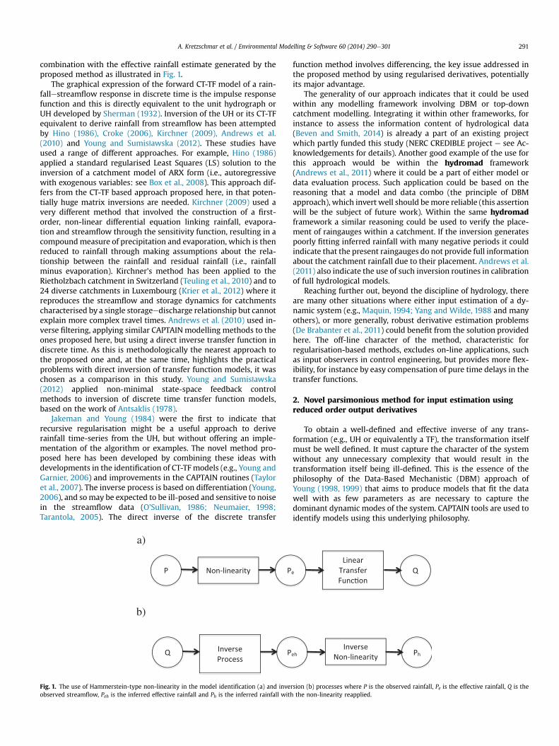
Fig. 2. Measured and estimated streamflow for: a) Baru (at 5 min intervals) and b) Blind Beck (at 15 min intervals), together with the associated hyetograms and impulse responses.

A. Kretzschmar et al. / Environmental Modelling & Software 60 (2014) 290e301294

compared visually with each other and with the observed rainfall.Inferred and observed rainfall series were then used as inputs to theoriginal forward models and the generated modelled flow se-quences compared using the Rt

2 values and visual comparisons.Statistical analysis of the residuals of both models gives an addi-tional insight into the differences between the catchments andrainfall regimes, as well as the differences between the inversionapproaches.

Model uncertainty is evaluated using Monte Carlo Simulations(MCS) for both the forward and the inverse models utilising thecovariance matrix generated as part of the output from the

estimation routines contained in the CAPTAIN Toolbox for Matlab(Taylor et al., 2007). In this analysis, the guidelines for validation ofDBM models published by Young (2001) are followed. The modelsthus generated can be used to investigate the sensitivity of theinversion process to the parameterisation of the forward model.

3.2. Data: Baru tropical catchment responses

The 0.44 km2 Baru catchment is situated in the headwaters ofthe Segama river located in Sabah on the northern tip of Borneo,East Malaysia (4� 580 N 117� 490 E). The climate is equatorial with a

Table 1The best CT-TF models fitted to subsets of data for Blind Beck (sampled at 15 minintervals) and Baru (sampled at 5 min intervals). There is little difference in effi-ciency (Rt2) between the different models so selectionwas based on the lowest ordermodel with the lowest YIC (Young, 2001). The YIC is an objectivemeasure combiningthe goodness of fit with a measure of over-parameterisation. A model with a largenegative YIC fits the data well with a small number of parameters.

Catchment Model structure[n,m,d]

Rt2 YIC Time constants (h)

1st 2nd

Blind Beck [2,2,3] 0.983 �6.711 6.35 22.10Baru [2,2,3] 0.878 �8.054 1.14 20.56

A. Kretzschmar et al. / Environmental Modelling & Software 60 (2014) 290e301 295

twenty-six year (1985e2010) mean rainfall of 2849 mm (Walshet al., 2011) showing no marked seasonality but tending to fall inshort (<15 min) convective events showing high spatial variabilityand intensities much higher than those of temperate UK (Bidin andChappell, 2003, 2006). Due to the high spatial variability, a networkof 6 automatic rain-gauges (13.6 gauges per km2) was used toderive the catchment-average rainfall using the Thiessen Polygonmethod. Haplic alisols, typically 1.5 m in depth and with a highinfiltration capacity (Chappell et al., 1998) are underlain by rela-tively impermeable mudstone bedrock resulting in the dominanceof comparatively shallow sub-surface pathways in this basin(Chappell et al., 2006). As a result of the high rainfall intensity andshallow water pathways the stream response is very flashy (i.e.,rapid recession in the impulse response function). The data used inthe analysis are from February 1996 sampled at 5 min intervals(Fig. 2a) and have been modelled previously by Chappell et al.(1999) and Walsh et al. (2011).

3.3. Data: Blind Beck temperate catchment response

The Blind Beck catchment has an area of 8.8 km2 and lies in theheadwaters of the Eden basin in North West England, UK (54.51�N2.38�W). The basin's response shows evidence of deep hydrologicalpathways due to the presence of deep limestone and sandstoneaquifers, and this has resulted in a damped hydrograph response(Mayes et al., 2006; Ockenden and Chappell, 2011; Ockenden et al.,2014). Winter rainfall in this basin is derived from frontal systemswith typically lower intensities than the convective systems in thetropics (Reynard and Stewart, 1993). Data from a single tipping-bucket raingauge (i.e., 0.1 gauges per km2) located in the middleof the catchment was used in this study. The data used in theanalysis covers the period from 26th Dec 2007 at 16:45 to 31stDecember 2007 at 21:45 sampled at 15 min intervals (Fig. 2b) andwas previously modelled by Ockenden and Chappell (2011).

The choice of these two experimental catchments, therefore,allowed the initial evaluation of the estimation of catchmentrainfall from streamflow for the end-member extremes of a basinwith tropical convective rainfall and shallow flow pathways to abasin with temperate frontal rainfall (i.e., much lower intensity)and deep flow pathways (i.e., much greater basin damping ortemporal integration).

4. First results and discussion

Forward CT-TF models identified for Blind Beck data explainedover 98% of the variance in the streamflow, whilst those for theBaru fit slightly less well, explaining 88% e see Table 1 for the Rt

2,YIC (Young, 2001), and time-constants of the best forward modelsfor each catchment, based on a high Rt

2 with a large negative YICvalue according to DBM methodology. The simulated streamflowsfrom a 2nd-order model for the two basins are shown in Fig. 2. Theimpulse response function (i.e., unit hydrograph) for the Baru

catchment (Fig. 2b) showed a considerably faster recession incomparison to that of the Blind Beck catchment (Fig. 2a) by a factorof 6, confirming the more flashy nature of the shallow, tropicalcatchment, as noted by previous transfer function studies (Chappellet al., 1999, 2006, 2012; Walsh et al., 2011).

The identifiedwell-fitting, forwardmodels selected according tothe DBM methodology were then inverted using the RegDermethod and, for comparison, the InvTF method to estimate catch-ment rainfall from streamflow for the two catchments. The resultsof the inversions using the two techniques are shown in Fig. 3 andthe reverse models' fit in Table 2.

Both approaches applied to the streamflow data for the BlindBeck catchment produced very similar inferred rainfall time-series(Fig. 3b). Both approaches produce slightly smoothed rainfall time-series compared to the observed 15-min sampled rainfall. Thesmoothing effect is small when compared with the time constant of6.4 h for the main component of the forward CT-TF model for theBlind Beck catchment (Table 1). Both produce some briefly negativerainfall values during periods of hydrograph recession. Estimatedperiods of negative rainfall are likely to be due to the point (i.e.,highly localised) rainfall measurements not fully characterising theentire catchment rainfall, so, at times, there is discharge with nolocally measured rainfall that could be attributed to it, and vice-versa; an effect also described by Young and Sumisławska (2012).

In general, the forward models fit very well so the uncertaintybounds demonstrated by Monte Carlo runs are very narrow asillustrated in Fig. 3.

When applied to the Baru data, the RegDer and InvTF approachesdo, however, give simulated or synthetic rainfall time-series withsome different characteristics (Fig. 3a). The InvTF method, whilecapturing some of the peaks better (illustrated in Fig. 4 and Table 3)gives a time-series with very high frequency noise component, ofsuch a high intensity that it produces momentary negative rainfallvalues. These very high frequency components are the result of thedirect differencing involved in this method of inversion, whichseverely amplifies high frequency noise in the signal. In contrast,the RegDer method again produced smoothed inferred rainfalltime-series with dynamics faster than the time constant of 1.14 hfor the faster component of the forward CT-TF model for the Barucatchment (Table 1). An interesting insight is gained by examiningthe inset in Fig. 3b, where the two inferred rainfall series clearlyfollow the same trajectory, but the InvTF results include the highfrequency noise, very clearly not related to the observed rainfall.The observed rainfall is indeed smoother than its InvTF estimate.These artefacts manifest themselves to a much higher degree in thefast responding Baru catchment with a different rainfall regime.

This last observation is confirmed by the residuals analysis.Residuals plots are shown in Fig. 3a and b for Baru and Blind Beckrespectively. It is apparent from the plots how much more highfrequency noise is involved in the InvTF estimates, even for theBlind Beck data, where both methods perform in a similar manner(see the residuals variance values in the plots). Fig. 5 showscomparative plots of the residuals autocorrelation function (RACF)for both models and both catchments. As expected the RACFs forBlind Beck are similar, quickly disappearing within their confidencebounds and it is just the variance level that differentiates the resultsfor both methods. For Baru the RACFs are quite different, with RACFfor RegDer quickly attenuated and not showing the negative ACFvalues characterising the fast switching, noisy InvTF residuals.

Table 3 shows that while the residuals statistics for Blind Beckshow good similarity between the methods, the residuals for Barushow large discrepancies, with InvTF showing some extreme valuesand a completely different distribution shape, as characterised bythe calculated moments: means are similar, variance doubles forInvTF, and higher moments are radically different and not realistic.

b)

a)

10 15 20 25 30 35 40 45 50 55 60

0

0.5

1

1.5

2

2.5

Time (hours)

Rai

nfal

l

Optimised NVR Regularised inversion

= 2.49e+00

measuredInvTF (223): Rt

2= 0.512

Optimised RegDer (223): Rt2=0.515

Percentile range

35 40 450

0.5

1

Time (hours)

Fig. 3. Comparison of rainfall simulated using the InvTF and RegDer (NVR optimised) methods for a) Baru and b) Blind Beck. Examination of the inset confirms that the RegDermethod estimates the Baru catchment rainfall better (see Table 2) whilst there is little difference between the methods for Blind Beck rainfall. 99% uncertainty bands generated byMonte Carlo analysis are shown and can be seen to be very narrow.

A. Kretzschmar et al. / Environmental Modelling & Software 60 (2014) 290e301296

The Mean Absolute Error statistics (MAE) show similar relation-ships to the variance.

Similar effects are shown by the peaks statistics (Bennett et al.,2013) in Fig. 6. In the figure Pe denotes effective rainfall, while Peh einferred effective rainfall. The errors in peak estimates are of similarmagnitude. Inferred in this figure refers to the values of peaks ofinferred rainfall. Baru results show considerable improvement ofthese peak error statistics achieved using RegDer approach.

Despite the presence of smoothing effects and/or high frequencynoise components, models simulating observed streamflow from

synthetic rainfall using either method were able to simulate theobserved streamflow equally well, and with a very high efficiency(Table 4), resulting in virtually indistinguishable model outputsgiven the observed rainfall or RegDer or InvTF rainfall as inputs. Thisis demonstrated in Fig. 7a and b.

It should be noted that while RegDer results appear to be ‘toosmooth’ and the InvTF resultse too ‘noisy’, the balance between thetwo is easily achieved using RegDer by balancing the NVR co-efficients of the inverse model, and will ultimately be up to theresearcher and the aims of modelling exercise. RegDer results can

Table 2Efficiency (Rt2) values for the rainfall sequences estimated by inverting the modelsselected for Blind Beck and Baru using the InvTF and RegDer methods of inversion.

Rt2 Blind Beck [2,2,3] Baru [2,2,3]

InvTF 0.512 �0.349RegDer 0.515 0.433

a)

b)

Fig. 4. Comparison of residuals for a) Baru and b) Blind Beck for the two inversion methods s(with a minor increase in noise for InvTF) and the differences when used for Baru (with lar

A. Kretzschmar et al. / Environmental Modelling & Software 60 (2014) 290e301 297

be interpreted as sub-sampling, or sacrificing the unobtainable(due to observation disturbance) temporal resolution. Critically,there are no such controls with InvTF. Quantifying this balance is apart of on-going research and is to be addressed in a forthcomingpublication. Applying a smoothing algorithm to InvTF results wouldproduce a different outcome, as RegDer only applies regularisationto the minimal number of terms within the bank of filters of

howing the similarities in performance between the methods when used for Blind Beckge artefacts in InvTF).

Table 3Residuals analysis for Blind Beck and Baru for both inversion methods showing the similarity between the methods for Blind Beck and the differences for Baru.

Mean Mode Var Skew Kurt Max Min Rng MAE

Blind BeckRegDer �0.0004 �0.0119 0.0549 2.54 20.1 1.71 �1.00 2.71 0.117InvTF 0.0001 �1.4012 0.0552 1.77 19.4 1.69 �1.40 3.09 0.118

BaruRegDer �0.004 0.0001 0.0459 3.51 112.3 4.09 �3.25 7.34 0.057InvTF �0.0036 0 0.1092 �27.17 1549.2 4.31 �19.56 23.9 0.066

a) b)

Fig. 5. Comparative plots of the residuals autocorrelation function (RACF) for InvTF (light grey bars) and RegDer (dark grey bars) and both catchments (Baru in (a) and Blind Beck in(b)) showing the differences between methods of inversion. In both cases, RegDer quickly attenuates whereas InvTF shows negative ACF values characterising the fast switching,noisy residuals/artefacts.

A. Kretzschmar et al. / Environmental Modelling & Software 60 (2014) 290e301298

Equation (5), as opposed to a cruder tool of smoothing the entiresignal.

The integrating effect of the Blind Beck catchment seen in thedamped hydrograph (Fig. 7b) was expected given the presence ofdeeper hydrological pathways (Ockenden and Chappell, 2011;

Fig. 6. Comparison of the estimation of peaks for the two methods showing that for Blind Bthem whilst for Baru, the InvTF method hugely underestimates the peak whilst RegDer slig

Ockenden et al., 2014) however, the degree of temporal basinintegration of the rainfall signal (and hence response damping) bythe shallow pathways within the tropical catchment (Chappellet al., 2006) was not expected, but does indicate the role of evenshallow water paths in damping intense rainfall. The degree of

eck, both methods estimate the observed peak quite well with little difference betweenhtly over-estimates. The metrics PDIFF and PEP were taken from Bennett et al. (2013).

Table 4Efficiency (Rt2) of forward CT-TF models of streamflow based on the observed rainfallor RegDer or InvTF rainfall as inputs.

Model input Blind Beck Rt2 Baru Rt

2

Observed rain 0.984 0.878Modelled rain (InvTF) 1.000 0.937Modelled rain (RegDer) 1.000 0.957

A. Kretzschmar et al. / Environmental Modelling & Software 60 (2014) 290e301 299

catchment integration indicates that the slight smoothing of thesimulated rainfall time-series (by the RegDer method) has noimpact on its ability to be used in forward CT-TF models to simulatestreamflow. On the basis of their utility for creating synthetic

b)

a)

150 2000

0.1

0.2

0.3

0.4

0.5

0.6

0.7

0.8

0.9

1

Tim

Dis

char

ge(Q

)

0123456789

10

Observed rainfallObserved flowModelled from observed rain Rt

2= 0.

Modelled from RD rain Rt2= 0.957

Modelled from InvTF rain Rt2= 0.937

0 20 40 60

0.05

0.1

0.15

0.2

0.25

0.3

0.35

Ra i

nfa l

l

Tim

Dis

char

ge(Q

)

0

1

2

3

4

Observed rainfallObserved flowModelled from observed rain Rt

2= 0.9

Modelled from RD rain Rt2= 1.000

Modelled from InvTF rain Rt2= 1.000

Fig. 7. Outputs modelled from observed and modelled rainfall sequences for a) Baru and b) Bfigure despite the differing characteristics of the rainfall inputs.

rainfall time-series for use in periods lacking observed rainfall, thenew RegDer method and InvTF method of Andrews et al. (2010)seem of equal value. Perhaps the new RegDer method is margin-ally better than the InvTF method because of the high frequencybehaviour that can be produced by the InvTF method with somedata sets where high frequency noise is amplified by the derivativeaction, for example, the proposed approach is more robust for stiffsystems (those with a wide range of time constants). Further, thishigh frequency behaviour has no physical interpretation so mightbe considered to fail the final evaluation criterion of the DBMmodelling philosophy (Chappell et al., 2012). These findings fromthe first evaluation of the new RegDermethod are very positive and

250 300 350e (hours)

878

195 200 2050

0.2

0.4

0.6

0.8

1

Time (hours)

0 80 100 120e (hours)

83

60 65 70 75 80 85 900

0.1

0.2

0.3

Time (hours)

lind Beck showing that the outputs (discharges) are indistinguishable over much of the

Table 5Data and model output statistics (rainfall). The following abbreviations were used: Var e variance, Kurt e kurtosis, Skew e skewness, IQR e inter-quartile range, Prct epercentiles. Obs refers to observed rainfall. The Wet prefix in the table rows refers to statistics calculated only for samples with non-zero rainfall (>0 for inferred).

Blind Beck Mean Var Skew Kurt Max Min Range 25% Prct 75% Prct IQR

Obs. all 0.181 0.112 3.154 15.934 2.476 0.003 2.474 0.004 0.233 0.230Obs. wet 0.181 0.112 3.152 15.925 2.476 0.000 2.476 0.004 0.233 0.230RegDer 0.182 0.061 1.744 7.451 1.576 �0.156 1.733 0.010 0.319 0.309InvTF 0.181 0.067 2.120 10.591 1.948 �0.198 2.146 0.008 0.311 0.303Wet RegDer 0.202 0.062 1.658 7.289 1.576 �0.129 1.705 0.012 0.342 0.330Wet InvTF 0.198 0.069 2.065 10.581 1.948 �0.198 2.146 0.010 0.345 0.335

BaruObs. all 0.050 0.081 11.230 179.694 6.853 0.000 6.853 0.000 0.000 0.000Obs. wet 0.253 0.403 4.383 27.969 6.056 0.000 6.056 0.000 0.213 0.213RegDer 0.054 0.054 7.549 76.584 3.674 �0.392 4.066 0.001 0.018 0.017InvTF 0.054 0.169 29.739 1411.93 23.374 �3.630 27.004 0.001 0.018 0.018Wet RegDer 0.055 0.042 6.751 60.481 2.763 �0.336 3.099 0.001 0.020 0.019Wet InvTF 0.051 0.095 18.517 567.320 12.644 �1.461 27.004 0.001 0.017 0.017

A. Kretzschmar et al. / Environmental Modelling & Software 60 (2014) 290e301300

highlight the potential value of this method for generating syn-thetic rainfall time-series for a range of rainfall regimes andcatchment settings. These preliminary findings have stimulated amuch more extensive programme of evaluation of the RegDermethod against a range of other methods (including the InvTFmethod of Andrews et al., 2010) for a much larger set of catchmentswith differing rainfall and catchment settings.

A number of basic statistics of the observed and inferred (RegDerand InvTF) rainfall series are shown in Table 5. It is clear that for theBlind Beck catchmentmost statistics for both observed and inferredseries are similar in magnitude (they were not expected to be tooclose due to the smoothing effect of both methods), which isconsistent with other results reported above. For Baru however,there are significant differences between the methods. There is anindication of mean-smoothing effects of both methods showing invariance and range. InvTF inferred rainfall shows large changes andunusual values in range, minima and maxima, as well as higherorder moments being of different order of magnitude from those ofthe actual rainfall and RegDer results. This is an indication of theartefacts of explicit differencing of the streamflow data when usingInvTF. In addition the high skewness of the observed rainfall mea-surements adds to the argument regarding non-Gaussian distri-bution, and hence many of the standard model metrics not beingapplicable.

5. Conclusions

Robust identification techniques were used to identifycontinuous-time transfer function models for two catchmentswith contrasting rainfall and flow path regimes. Following theDBM methodology, the models fitted the data well with a minimalnumber of parameters as indicated by a large negative value of theYIC. The identified (DBM) models for both catchments were of 2nd-order. This is a typical model order for many catchments. Themodels were inverted using the new RegDer method and, forcomparison, the InvTF method used by Andrews et al. (2010). Bothmethods were able to produce synthetic rainfall time-series thatwere then able to simulate almost all of the dynamics in thestreamflow time-series for both catchments (Fig. 4a, b). In com-parison to the InvTF method of Andrews et al. (2010), the RegDermethod did, however, produce synthetic rainfall containing muchless high frequency noise. This was particularly visible in thesynthetic rainfall of InvTF for the tropical basin with convectiverainfall (Fig. 3a). The smoothing introduced by the RegDer methodis on a much smaller temporal scale than the dominant dynamicsof the catchment indicating that the detailed temporal distributionof the rainfall series may not be important for the modelling the

observed streamflow (depending on the reasons for modelling) solong as the series recreates the short-term (i.e., sub-hourly) char-acteristics responsible for producing stream hydrographs suffi-ciently well, which is consistent with the findings of Eagleson(1967) and Obled et al. (1994). These findings are confirmed bycomparative evaluation of several model metrics, including peakmodelling errors and a detailed residuals analysis. It is worthnoting that applying a smoothing algorithm to InvTF results wouldproduce a different outcome, as RegDer only applies regularisationto the minimal number of terms within the bank of filters ofEquation (5), as opposed to a cruder tool of smoothing the entiresignal.

Further evaluations of the new RegDermethod against InvTF andothermethods need to be undertaken using amore diverse range ofglobal rainfall and flow-path regimes. This work will includecatchments where the derivation of long-term rainfall time-seriesby RegDer would support hydrological, climatological or ecolog-ical studies requiring such long time-series of synthesised rainfall(Ormerod and Durance, 2009).

Software and data used to produce the results in this paper areavailable upon request from the corresponding author.

Acknowledgements

The authors would like to thank Mary Ockenden for thecollection and quality assurance of the period of rainfall andstreamflow for the Blind Beck catchment (NERC grant number NER/S/A/2006/14326), and also Jamal Mohd Hanapi and Johnny Larenusfor the collection of the period of rainfall and streamflow utilisedfor the Baru catchment and to Paul McKenna for its quality assur-ance (NERC grant number GR3/9439). This work has been partlysupported by the Natural Environment Research Council [Con-sortium on Risk in the Environment: Diagnostics, Integration,Benchmarking, Learning and Elicitation (CREDIBLE)] grant number:NE/J017299/1.

References

Alexandrov, G.A., Ames, D., Bellocchi, G., Bruen, M., Crout, N., Erechtchoukova, M.,Hildebrandt, A., Hoffman, F., Jackisch, C., Khaiter, P., Mannina, G., Matsunaga, T.,Purucker, S.T., Rivington, M., Samaniego, L., 2011. Technical assessment andevaluation of environmental models and software: letter to the editor. Environ.Model. Softw. 26 (3), 328e336.

Anderssen, R., Bloomfield, P., 1974. Numerical differentiation procedures for non-exact data. Numer. Math. 22, 157e182.

Andrews, F., Croke, B., Jeanes, K., 2010. Robust estimation of the total unit hydro-graph. In: 2010 International Congress on Environmental Modelling and Soft-ware Modelling for Environment's Sake. Ottawa, Canada.

A. Kretzschmar et al. / Environmental Modelling & Software 60 (2014) 290e301 301

Andrews, F., Croke, B., Jakeman, A., 2011. An open software environment for hy-drological model assessment and development. Environ. Model. Softw. 26 (10),1171e1185.

Antsaklis, P., 1978. Stable proper nth-order inverses. IEEE Trans. Autom. Control 23(6), 1104e1106.

Bardossy, A., Das, T., 2008. Influence of rainfall observation network on modelcalibration and application. Hydrol. Earth Syst. Sci. 12 (1), 77e89.

Bennett, N.D., Croke, B.F.W., Guariso, G., Guillaume, J.H.A., Hamilton, S.H.,Jakeman, A.J., Marsili-Libelli S,Newham, L.T.H., Norton, J.P., Perrin, C., Pierce, S.A.,Robson, B., Seppelt, R., Voinov, A.A., Fath, B.D., Andreassian, V., 2013. Charac-terising performance of environmental models. Environ. Softw. 40, 1e20.

Beven, K., 2006. A manifesto for the equifinality thesis. J. Hydrol. 320, 18e36.Beven, Keith J., 2011. RainfalleRunoff Modelling e the Primer, second ed. John

Wiley and Sons, Chichester, England.Beven, K., Smith, P., 2014. Concepts of information content and likelihood in

parameter calibration for hydrological simulation models. J. Hydrol. Eng. 10,1061.

Bidin, K., Chappell, N., 2003. First evidence of a structured and dynamic spatialpattern of rainfall within a small humid tropical catchment. Hydrol. Earth Syst.Sci. 7 (2), 245e253.

Bidin, K., Chappell, N., 2006. Characteristics of rain events at an inland locality inNortheastern Borneo, Malaysia. Hydrol. Process. 20 (18), 3835e3850.

Box, G.E.P., Jenkins, G.M., Reinsel, G.C., 2008. Time Series Analysis: Forecasting andControl, fourth ed.

Bryson, A.E., Ho, Y.-C., 1969. Applied Optimal Control: Optimization, Estimation, andControl.

Chappell, N., Franks, S., Larenus, J., 1998. Multi-scale permeability estimation for atropical catchment. Hydrol. Process. 12 (9), 1507e1523.

Chappell, N.A., Mckenna, P., Bidin, K., Douglas, I., Walsh, R.P.D., 1999. Parsimoniousmodelling of water and suspended sediment flux from nested catchmentsaffected by selective tropical forestry. Philos. Trans. R. Soc. Lond. Ser. B Biol. Sci.354 (1391), 1831e1846.

Chappell, N.A., Tych, W., Chotai, A., Bidin, K., Sinun, W., Chiew, T.H., 2006. Bar-umodel: combined data based mechanistic models of runoff response in amanaged rainforest catchment. For. Ecol. Manag. 224 (1), 58e80.

Chappell, N.A., Bonell, M., Barnes, C., Tych, W., 2012. Tropical cyclone effects onrapid runoff responses: quantifying with new continuous-time transfer func-tion models. In: Webb, A.A., Bonell, M., Bren, L., Lane, P.N.J., Mcguire, D.,Neary, D.G., Nettles, J., Scott, D.F., Stednick, J., Wang, Y. (Eds.), RevisitingExperimental Catchment Studies in Forest Hydrology: Proceedings of a Work-shop Held during the XXV IUGG General Assembly in Melbourne. JuneeJuly2011. International Association of Hydrological Sciences (IAHS), Wallingford.

Croke, B., 2006. A technique for deriving an average event unit hydrograph fromstreamflow e only data for ephemeral quick-flow-dominant catchments. Adv.Water Resour. 29 (4), 493e502.

Cunha, L., Mandapaka, P., Krajewski, W., Mantilla, R., Bradley, A., 2012. Impact ofradar-rainfall error structure on estimated flood magnitude across scales: aninvestigation based on a parsimonious distributed hydrological model. WaterResour. Res. 48.

De Brabanter, K., De Brabanter, J., De Moor, B., 2011. Nonparametric derivativeestimation. In: Proceedings of the 23rd Benelux Conference on ArtificialIntelligence.

Eagleson, P., 1967. Optimum density of rainfall networks. Water Resour. Res. 3 (4),1021.

Fujihara, Y., Simonovic, S., Topaloglu, F., Tanaka, K., Watanabe, T., 2008. An inverse-modelling approach to assess the impacts of climate change in the Seyhan RiverBasin, Turkey. Hydrol. Sci. J.-J. Des. Sci. Hydrol. 53 (6), 1121e1136.

Hino, M., 1986. Improvements in the inverse estimation of effective rainfall fromrunoff. J. Hydrol. 83 (1e2), 137e147.

Hjelmfelt, A., 1981. Overland flow from time-distributed rainfall. J. Hydraul. Div.-ASCE 107 (2), 227e238.

Jakeman, A., Young, P., May 1984. Recursive filtering and smoothing procedures forthe inversion of ill-posed causal problems. Util. Math. 25, 351e376.

Kalman, R.E., 1960. A new approach to linear filtering and prediction problems.Trans. ASME J. Basic Eng. 82 (Series D), 35e45.

Kirchner, J., 2009. Catchments as simple dynamical systems: catchment charac-terization, rainfallerunoff modeling, and doing hydrology backward. WaterResour. Res. 45.

Krier, R., Matgen, P., Goergen, K., Pfister, L., Hoffmann, L., Kirchner, J.W.,Uhlenbrook, S., Savenije, H.H.G., 2012. Inferring catchment precipitation bydoing hydrology backward: a test in 24 small and mesoscale catchments inLuxembourg. Water Resour. Res. 48, W10525.

Littlewood, I., Croke, B., 2013. Effects of data time-step on the accuracy of calibratedrainfall-streamflow model parameters: practical aspects of uncertainty reduc-tion. Hydrol. Res. 44 (3), 430e440.

Luo, Jianwen, Ying, Kui, Bai, Jing, 2005. SavitzkyeGolay smoothing and differenti-ation filter for even number data. Signal Process. 85 (7), 1429e1434.

Maquin, 1994. Estimation of unknown inputs in linear systems. In: AmericanControl Conference, ISBN 0-7803-1783-1, pp. 1195e1197.

Mayes, W.M., Walsh, C.L., Bathurst, J.C., Kilsby, C.G., Quinn, R.F., Wilkinson, M.E.,Daugherty, A.J., Connell, P.E., 2006. Monitoring a flood event in a denselyinstrumented catchment, the Upper Eden, Cumbria, UK. Water Environ. J. 20(4), 217e226.

Moussaoui, S., Brie, D., Richard, A., 2005. Regularization aspects in continuous-timemodel identification. Automatica 41 (2), 197e208.

Neumaier, A., 1998. Solving ill-conditioned and singular linear systems: a tutorial onregularization. SIAM Rev..

Norton, J.P., 2009. An Introduction to Identification. Dover Publications.O'Sullivan, F., 1986. A statistical perspective on ill-posed inverse problems. Stat. Sci.

1 (4), 502e518.Obled, C., Wendling, J., Beven, K., 1994. The sensitivity of hydrological models to

spatial rainfall patterns e an evaluation using observed data. J. Hydrol. 159(1e4), 305e333.

Ockenden, M.C., Chappell, N.A., 2011. Identification of the dominant runoff path-ways from data-based mechanistic modelling of nested catchments intemperate UK. J. Hydrol. 402 (1), 71e79.

Ockenden, M.C., Chappell, N.A., Neal, C., 2014. Quantifying the differential contri-butions of deep groundwater to streamflow in nested basins, using both waterquality characteristics and water balance. Hydrol. Res. 45, 200e212.

Ogden, F., Julien, P., 1994. Runoff model sensitivity to radar resolution. J. Hydrol. 158(1e2), 1e18.

Ormerod, S., Durance, I., 2009. Restoration and recovery from acidification in up-land Welsh streams over 25 years. J. Appl. Ecol. 46 (1), 164e174.

Reynard, N.S., Stewart, E.J., 1993. The derivation of design rainfall profiles for uplandareas of the UK. Meteorol. Mag. 122, 116e123.

Sherman, L.K., 1932. Streamflow from rainfall by the unitgraph method. Eng. NewsRec. 108, 501e505.

Tarantola, A., 2005. Inverse Problem Theory and Methods for Model ParameterEstimation: Society for Industrial and Applied Mathematics.

Taylor, C.J., Pedregal, D.J., Young, P.C., Tych, W., 2007. Environmental time seriesanalysis and forecasting with the Captain toolbox. Environ. Model. Softw. 22 (6),797e814.

Teuling, A.J., Lehner, I., Kirchner, J.W., Seneviratne, S.I., 2010. Catchments as simpledynamical systems: experience from a Swiss prealpine catchment. WaterResour. Res. 46 (10).

Tych, W., Pedregal, D.J., Young, P.C., Davies, J., 2002. An unobserved componentmodel for multi-rate forecasting of telephone call demand: the design of aforecasting support system. Int. J. Forecast. 18 (4), 673e695.

Walsh, R.P.D., Bidin, K., Blake, W.H., Chappell, N.A., Clarke, M.A., Douglas, I.,Ghazali, R., Sayer, A.M., Suhaimi, J., Tych, W., Annammala, K.V., 2011. Long-termresponses of rainforest erosional systems at different spatial scales to selectivelogging and climatic change. Philos. Trans. R. Soc. Lond. 366, 3340e3353.

Wang, W., Henriksen, R., 1994. Generalized predictive control of nonlinear systemsof the Hammerstein form. Model. Identification Control 15 (4), 253e262.

Yang, F., Wilde, R., 1988. Observer for linear systems with unknown inputs. IEEETrans. Autom. Control 33 (7), 677e681.

Young, P.C., 1998. Data-based mechanistic modelling of environmental, ecological.Econ. Eng. Syst. 13 (2), 105e122.

Young, P.C., 1999. Data-based mechanistic modelling. Gen. Sensit. Domin. ModeAnal. 117 (1e2), 113e129.

Young, P.C., 2001. Data-based mechanistic modelling and validation of rainfall-flowprocesses. In: Anderson, M.G., Bates, P.D. (Eds.), Model Validation: Perspectivesin Hydrological Science. J. Wiley, Chichester, pp. 117e161.

Young, P.C., 2006. Data-based mechanistic modelling and river flow forecasting. In:14th IFAC Symposium on System Identification, pp. 756e761. Newcastle,Australia.

Young, P., Garnier, H., 2006. Identification and estimation of continuous-time, data-based mechanistic (DBM) models for environmental systems. Environ. Model.Softw. 21 (8), 1055e1072.

Young, P.C., Jakeman, A., 1980. Refined instrumental variable methods of recursivetime-series analysis, part III. Extensions. Int. J. Control 31 (4), 741e764.

Young, P.C., Sumisławska, M.A., 2012. Control systems approach to input estimationwith hydrological applications. In: 16th IFAC Symposium on System Identifi-cation. July 2012, Brussels, Belgium, pp. 1043e1048.

Young, P.C., Pedregal, D.J., Tych, W., 1999. Dynamic harmonic regression. J. Forecast.18 (6), 369e394.

Yu, B., Ciesiolka, C., Rose, C., Coughlan, K., 1997. Note on sampling errors in therainfall and runoff data collected using tipping bucket technology. Trans. ASAE40 (5), 1305e1309.