Reverse Supply Chain Management - Modeling Through …cdn.intechopen.com/pdfs/18519/InTech-Reverse_supply_chain_management... · 20 Reverse Supply Chain Management - Modeling Through

20

Reverse Supply Chain Management - Modeling Through System Dynamics

Rafael Rodríguez-Fernández, Beatriz Blanco, Adolfo Blanco and Carlos A. Perez-Labajos

University of Cantabria Spain

1. Introduction

Supply Chain Management (SCM) is one of the disciplines of Operations Management that has developed the most over the last few years. Within Supply Chain Management, Green Supply Chain Management (GSCM) is a relatively young area which has great prospects for the future, due to the increasing deterioration in the environment, the shortage of material resources, the overfilling of rubbish dumps, the increase in pollution levels, the requirements of the legislation and the pressures of consumers ever more aware of the environment. One of the areas of most interest in the study of GSCM is Reverse Logistics. Many experts have adopted the slogan of "the three Rs" (Reduce, Reuse, Recycle) to promote environmental awareness in the production process. Reprocessing is a combination of "the three R's" in one same activity (Ferrer 2001). Examples of items that can be directly reused without prior repair (except for cleaning and a minimum maintenance) are returnable packaging like bottles, pallets, and containers. In some businesses, customers have the legal right to return products purchased within a specific space of time. In these cases, the money is refunded in whole or in part and the product can be resold if it is of sufficient quality and if there is still demand for it (Mostard, Teunter 2006). Personal computers can be reused by replacing their hard disks, processors, by adding extra memory or a modem for internet, and even screens, keyboards and memories can be sold on to a toy company (Inderfurth, de Kok & Flapper 2001). The packaging returned to companies is generally reused. Pallets and containers can often be restored and returned for reuse (Rogers, Tibben-Lembke 1999). The goal of repair is to restore a product that has failed to make it work properly again with a slight loss of quality. Some examples are household appliances, industrial machinery and electronic equipment. Recycling involves the recovery of material without maintaining the original structure of the product. Examples of recyclable materials are paper, glass and plastics. Reprocessing retains the identity of the original product with the aim of making the product “like new” again by disassembling, upgrading and replacing the appropriate parts. Examples of items that can be reprocessed are airplanes, machine tools and photocopying-machines.

2. Legislative pressure

Many industrialized countries in Europe have strengthened their environmental legislation by laying the responsibility for reverse logistics flows, including used products and waste products, in the hands of the manufacturers (Fleischmann et al. 2000).

www.intechopen.com

Supply Chain Management - New Perspectives

418

There are numerous ways to minimize the environmental costs of production, but the prevention of waste from the products eliminates many environmental costs before they occur. A material recovery system, based on environmentally recoverable products, includes strategies for increasing the lifespan of products consisting in the repair, reprocessing and recycling of products (Jayaraman, Guide & Srivastava 1999). Waste reduction has received increasing attention in industrialized countries in view of the exhaustion of the capacity of landfills and incineration. One of the most widely used measures is that of the obligation to return products after use. In Germany, for example, the packaging law of 1991 requires industries to recover the packaging of the products sold and imposes a minimum percentage of recycling. The electronic equipment law of 1996 establishes similar recycling targets for electronic products. In the Netherlands, the automobile industry is responsible for the recycling of all used cars (Cairncross 1992, in (Fleischmann et al. 1997)). But even where the legislation is not so strict, the expectations of consumers put a lot of pressure on companies to take into account environmental aspects (Vandermerwe and Oliff, 1990 at (Fleischmann et al. 1997)). A "green" image has become an important element of marketing. To comply with this legislation, several German companies developed the Dual System Deutschland ("DSD") in order to meet quotas for the recycling of different types of packaging. The European Commission presented a set of bills on the collection and recycling of electrical and electronic waste in April 1998. This law sets targets for waste electrical and electronic equipment ("WEEE"), to increase recycling, reduce hazardous substances, and to make the waste safer. The standard includes a wide variety of electronic products such as mobile phones, video games, toys, domestic appliances and office equipment. Norway has announced plans to require manufacturers and importers of electronic equipment (EE) to collect the used products and waste materials. Half a dozen enterprises have undertaken to collect 80% of EE waste in Norway. Following the principle of "the polluter pays", the system will be financed by a tax on new electronic products. In some industries, it is the government that does the collecting, as in the Swedish battery industry. In some cases, installation networks are organized and used by the industry as in the case of the Swedish automobile industry and in other cases, companies must set up their own collection centers.

3. System dynamics: Concept, origins and applications

One of the most widely accepted definitions is the one proposed by Wolstenholme (Wolstenholme 1990, in (Pérez Ríos 1992)): “System Dynamics is a rigorous method for qualitative description, exploration and analysis of complex systems in terms of their processes, information, organizational boundaries and strategies; which facilitates quantitative simulation, modeling and analysis for the design of the system structure and control”. In the 1950s, Jay Forrester, a systems engineer at MIT, was commissioned by the US company Sprague Electrics to study the extreme oscillations of their sales and establish a means to correct them. From previous experience, Forrester knew the essence of the problem stemmed from the oscillations present in situations that contain inertia effects, or delays and reverse effects, or feedback loops as basic structural characteristics. In 1961, Forrester published his work “Industrial Dynamics“ (Forrester 1961) which marks the beginning of the “System Dynamics” technique as a procedure for the study and

www.intechopen.com


419

simulation of the behavior of social systems. In 1969, the work “Urban Dynamics” was published, explaining how system dynamics modeling is applicable to city systems. “World Dynamics“ or “The World of Work“ appeared in 1970, a work that served as a basis for Meadows and Meadows to make the first report to the Club of Rome, a work which was published with the name of Limits to Growth (published in Spanish by the Fondo de Cultura Económica, México, 1972). The great merit of this book is that it was published a year before the raw materials crisis of 1973, and that it foresaw in part its consequences. This work popularized Systems Dynamics on a worldwide scale. At present, Systems Dynamics is a widely used technique for modeling and studying the behavior of all types of systems which have the above-mentioned characteristics of delays or feedback loops. These characteristics are especially pronounced and intense in social systems so that these systems often show unexpected and unpredictable behavior. System dynamics is applied in a wide range of fields. During its more than 40 years of existence, it has been used to build computer simulation models in almost all of the sciences, such as business administration, urban planning, engineering and in sociological systems where it has found many applications, from more theoretical aspects such as the social dynamics of Pareto and Marx, to issues of the implementation of justice. One area in which several important applications have been developed is that of environmental and ecological systems, focusing on problems of population dynamics and the spread of pollution. Another interesting field of application is that of energy supply systems, where it has been used to define strategies for the use of energy resources. It has also been used for defense issues, simulating logistical problems of the evolution of troops and other similar problems. The system dynamics perspective is radically different from that of other techniques applied to the modeling of socioeconomic systems, such as econometrics. Econometric techniques, based on a behavioral approach, use empirical data as the basis of statistical calculations in order to determine the meaning and correlation between different factors. The evolution of the model is based on the past performance of the so-called independent variables, and statistics is applied to determine the parameters of the system of equations that relate these to the other so-called dependent variables. These techniques seek to determine the behavior of the system without entering into the knowledge of their internal mechanisms. Thus, many models for investing in the stock market analyze the peaks and valleys in the prices, the boom and bust cycles, etc. and design strategies to minimize the risk of loss, etc. They do not, then, attempt to “know” why a company’s market value rises or falls as a function of its new products, new competitors, etc. In contrast, the basic aim of System Dynamics is to work out the structural causes that provoke the behavior of the system. This involves increasing awareness of the role of each element of the system and seeing how different actions, performed on the parts of the system, intensify or attenuate its implicit behavioral tendencies. Since its first appearance, there have been numerous applications of system dynamics to corporate policies and strategic issues, though few publications have applied system dynamics to the supply chain and most of these have been applied to the direct supply chain. Forrester (Forrester 1961) includes a supply chain model as an early example of applying the system dynamics methodology. Towill (Towill 1995 in (Vlachos, Georgiadis & Iakovou 2007)) applies system dynamics to the redesign of the supply chain. Minegishi and Thiel (Minegishi and Thiel (2000) in (Vlachos, Georgiadis & Iakovou 2007)) apply system dynamics to improve understanding of the complex behavior of logistics in an integrated

www.intechopen.com


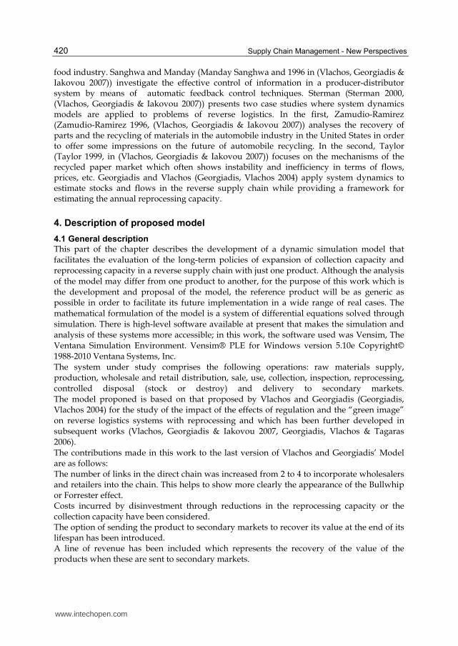
420

food industry. Sanghwa and Manday (Manday Sanghwa and 1996 in (Vlachos, Georgiadis & Iakovou 2007)) investigate the effective control of information in a producer-distributor system by means of automatic feedback control techniques. Sterman (Sterman 2000, (Vlachos, Georgiadis & Iakovou 2007)) presents two case studies where system dynamics models are applied to problems of reverse logistics. In the first, Zamudio-Ramirez (Zamudio-Ramirez 1996, (Vlachos, Georgiadis & Iakovou 2007)) analyses the recovery of parts and the recycling of materials in the automobile industry in the United States in order to offer some impressions on the future of automobile recycling. In the second, Taylor (Taylor 1999, in (Vlachos, Georgiadis & Iakovou 2007)) focuses on the mechanisms of the recycled paper market which often shows instability and inefficiency in terms of flows, prices, etc. Georgiadis and Vlachos (Georgiadis, Vlachos 2004) apply system dynamics to estimate stocks and flows in the reverse supply chain while providing a framework for estimating the annual reprocessing capacity.

4. Description of proposed model

4.1 General description

This part of the chapter describes the development of a dynamic simulation model that facilitates the evaluation of the long-term policies of expansion of collection capacity and reprocessing capacity in a reverse supply chain with just one product. Although the analysis of the model may differ from one product to another, for the purpose of this work which is the development and proposal of the model, the reference product will be as generic as possible in order to facilitate its future implementation in a wide range of real cases. The mathematical formulation of the model is a system of differential equations solved through simulation. There is high-level software available at present that makes the simulation and analysis of these systems more accessible; in this work, the software used was Vensim, The Ventana Simulation Environment. Vensim® PLE for Windows version 5.10e Copyright© 1988-2010 Ventana Systems, Inc. The system under study comprises the following operations: raw materials supply, production, wholesale and retail distribution, sale, use, collection, inspection, reprocessing, controlled disposal (stock or destroy) and delivery to secondary markets. The model proponed is based on that proposed by Vlachos and Georgiadis (Georgiadis, Vlachos 2004) for the study of the impact of the effects of regulation and the “green image” on reverse logistics systems with reprocessing and which has been further developed in subsequent works (Vlachos, Georgiadis & Iakovou 2007, Georgiadis, Vlachos & Tagaras 2006). The contributions made in this work to the last version of Vlachos and Georgiadis’ Model are as follows: The number of links in the direct chain was increased from 2 to 4 to incorporate wholesalers and retailers into the chain. This helps to show more clearly the appearance of the Bullwhip or Forrester effect. Costs incurred by disinvestment through reductions in the reprocessing capacity or the collection capacity have been considered. The option of sending the product to secondary markets to recover its value at the end of its lifespan has been introduced. A line of revenue has been included which represents the recovery of the value of the products when these are sent to secondary markets.

www.intechopen.com


421

Figures 1 and 2 show respectively the causal diagram and flowchart of the proposed model. Figure 3 shows the flowchart of the cost and revenue model. The description of the variables, ordered alphabetically, is presented in Annex 1. The model equations are set out in Annex 2.

4.2 Explanation of causal diagram

The direct chain begins with the procurement of raw materials (MP) from suppliers. The production ratio (PR) is determined using the stock management structure proposed by Sterman (Sterman 1989). Thus, the of production ratio (PR) is obtained by combining the difference between the expected demands of the distributors (EDO) and the expected reprocessing ratio (RER) with the adjustment provided by the useful inventory (UI), depending on its desired value (UIDE). The production ratio (PR) is limited by the production capacity (PC). The useful inventory (UI) consists of new products through the production ratio (PR), which introduces new products according to their production time (PT) and reprocessed products (REP) through the reprocessing ratio (RPR), which introduces reprocessed products according to their reprocessing time (RPT). Through the useful inventory (UI), the intention is to cover as far as possible the orders from the distributors (OB) through deliveries to the distributors (SD), which, in terms of time, means the delivery time taken to reach the distributors (DST) increasing at this rate the distributors’ inventory (DI). The distributors’ orders (OB) are made in keeping with the control rule given by Sterman (Sterman 1989). This process is repeated in the same way in the links of the wholesalers and retailers, except that in these cases, rather than linking the useful inventory (UI) with the distributors’ inventory (DI), the distributors’ inventory (DI) will be linked with that of the wholesalers (MI) and the wholesalers’ inventory (MI) will be connected to the retailers’ inventory (RI). All unmet orders become backorders which are satisfied after a period of time. The retail inventory (RI) attempts to meet demand (D) through sales (S), just as the backorder (DB) is satisfied after a period of time (DCT). The demand (D) has been represented by the life cycle of the generic product. The sales (S), after their residency period (RT), become used goods (UP) that can be collected for reuse (CP) or disposed of in an uncontrolled manner (UDP and UD). The reverse chain starts with the collected products (CP), which increase in keeping with the

collection ratio (CR), which is limited by the collection capacity (COR), and decrease as the

products are accepted for reuse (PARU) or rejected (PRR). The stock of reusable products

(REP) is used for reprocessing if the reprocessing capacity (RPC), which limits the

reprocessing ratio (RPR), is adequate.

To prevent the uncontrolled accumulation of reusable products (REP), the option of sending

the products to controlled disposal (CD) has been proposed, if these are not used after a

specified time of maintenance of reusable stock (RSKT). This also means that the products

that go to be reprocessed are as recent as possible.

Once the demand (D) of the direct chain for the product falls, provision is made for the

liquidation of the inventories of all of the direct supply chain members to send the product

directly to the secondary markets (SMPO), thus recovering part of their value.

The collection capacity (COR) is revised at every stage in the simulation time so that it is

virtually continuous and the decision to be made is whether to invest or disinvest in the

collection capacity (COR) and to what extent. The ratios of expansion (CCIR) or contraction

(CCRR) of the collection capacity depend on the discrepancy (CCDI) between the desired

www.intechopen.com


422

collection capacity (CCDE) and the current collection capacity (COR). The desired collection

capacity (CCDE) is forecast based on time series of used products (UP). The magnitude of

each expansion (CCER) or contraction (CCCR) is proportional to the discrepancy in the

collection capacity (CCDI) at a given time and a lower limit has been established to prevent

small changes from occurring very frequently.

The discrepancy in the collection capacity (CCDI) is multiplied by a parameter Kc1 for

expansion and Kc2 for contraction, thus characterizing the two strategies for the

planning of the collection capacity (COR). The strategies with high Kc1 and Kc2 values

are more aggressive than those with lower values; however, in all cases, there is a time

lapse (Tc1 and Tc2) between the time the decision is made and that of its effective

implementation.

The ratio of the increase in collection capacity (CCIR) and the ratio of the reduction in

collection capacity (CCRR) takes into consideration this time delay for the expansion in the

collection and reduction capacities, respectively.

The causal diagram for the reprocessing capacity (RPC) is similar, the only difference being

that the used products (UP) are replaced by Sales x (1-percent defective products) (Sx(1-FP)),

which is used to forecast the desired reprocessing capacity (RCDE). The rest of the variables

(Kr1,Kr2, Tr1, Tr2…) fulfil the same function as their equivalents in the collection capacity

(Kc1,Kc2, Tc1, Tc2…)

The justification for using different sources of information in determining the collection

(COR) and reprocessing (RPC) capacities lies in the fact that the objectives of these two

operations are different. The purpose of the collection is twofold:

To supply the reprocessing process

To ensure the controlled disposal of the used products at the end of their useful life.

The aim of reprocessing is to satisfy the major part of the demand (D); thus, the reprocessing

capacity (RPC) is of no use at the end of the life cycle of the product. This explains why the

desired reprocessing capacity (RCDE) is linked to the sales (S) and the desired collection

capacity (CCDE) is linked to the used products (UP).

Figure 1 shows the causal diagram used in the conceptual part of the model. This is a

useful diagram for establishing relationships between the different variables. The

relationships shown are of two types: the links indicated by a continuous line

correspond to material flows and those represented by dashed lines correspond to

information flows.

The nature of the links has also been considered, indicating with a "+" sign direct relations,

that is those in which there is a direct proportionality, meaning that when one of the

variables increases, the one linked to it also increases (+) and vice versa - if the value of the

variable decreases the one linked to it (+) also decreases. The complementary case is

indicated by a (-) sign, meaning that the relation is proportionally inverse: that is, when one

of the variables increases, the one linked to it (-) decreases and vice versa – if the value of the

variable decreases, the one linked to it increases.

Since it is generated in the design stage of the model, the causal diagram does not include

some of the parameters that will be required later in the modelling phase (Tc1, Tc2, a-

CC…). Nor does it indicate the nature of the flow or the level of each variable. All of this

information is included when the model is made and the Forrester diagram or flow diagram

is generated (fig.2).

www.intechopen.com


423

MP UI DI

RPCREP

DP

CP

COR

UDP

OBPC

PT

UIAT

UID

-

UIDE-

UICT

+

DIAT

DID

-

MST

DIDE

+

DICT

+

EMO

+EDO

+

DSTRER

RPT

RCER

Kr1

RPCD

RCDE

+

-

+

+

RSKT

IT

FPCCER

Kc1

CCDI

+

+

-

CCDE

+

CCCR

Kc2

+

RT

RCCRKr2

+

+UP

+

+

+-

-

MI RI

ROBMIDI

-

MIDE

+

MICT

+

RIAT

RIDI

-

DCT

RIDE+

RICT

+

ED

+ERO

+

RST

DB

MBO

MIAT

SMPO

PR

+ ++

--

-

+-+

+

+ +

+

SD+-

-+

-+

DO

+

+

+

+

+

MO

+

+

++

+

MS+-

-+

+-

RS+-

-

+

- +

RO

+

+

+

++

D

+

+

S+-

-

+

-

+

+

UD+

+

CR +

+

-+

CCIR

+

+

CCRR

+PRR

+

-

-

+

+

PARU

+

-

--

+

CD

+

-

+

-

RPR+

-

-

+

+

RCIR

+

+

RCRR

+-

-

Fig. 1. Causal diagram of the proposed model. (Information on variables in Annex 1 and model ecuations in Annex 2)

Figure 2 shows the flow chart of the model. In this case, the material flows are represented by double-line arrows and the information flows by single line arrows.The chart below now includes all the variables involved in the model and indicates their nature: The level variables are represented inside rectangles. These variables have an accumulation of material and therefore are linked to material lines. The flow variables are those that indicate the variation of the level variables and are represented by a hydraulic wrench symbol. The rest of the elements of the model are variables without accumulation and parameters. Figure 3 shows the flow chart of the economics part of the model. On the left are shown all the operating costs associated with the model which are: Weekly cost of useful inventory storage (UISWCOST), weekly cost of transport to distributors (DTWCOST), weekly storage cost of distributors (DISWCOST), weekly cost of transport to wholesalers (MTWCOST), weekly cost of wholesalers’ inventory storage (MISWCOST), weekly cost of retailers’ inventory storage (MSIWCOST), weekly cost of transport to retailers (RTWCOST), weekly cost of transport of sales (STWCOST), weekly cost of reusable product storage (RSPWCOST), weekly production cost (WPCOST), weekly cost of reusable storage (RPWCOST) and weekly cost of collection (CWCOST). On the right are represented the

www.intechopen.com


424

investment costs of the model: weekly collection capacity cost (CCWCOST) and weekly reprocessing capacity cost (RCWCOST). At the bottom are shown the sales revenue of the model (SI) and the various revenues from inventory liquidation (PLIR, DILI, MILI, ILPIs). The net present value of the entire supply chain (NPVWN) is represented in the centre of the figure.

MP UI DI

RPC

REP

DP

CP

COR

UDP

OB

PR SD

DOOBRR

RCIR

PARU

CD

PRR

CCIR

UD

PC

PT

UIAT

RPR

UID

UIDE

UICT

DIAT

DID

MST

DIDE

DICT

EMO

a-MI

EDO

a-DI

DSTRER

a-RR

RPT

RCER Kr1

RPCD

RCDE

a-RPC

RSKT

IT

FP

CCERKc1

CCDI

CCDE

a-CC

CCRR

CCCR

Kc2

lbc

PD

Tc1

Tc2

RT

RCRR

Tr1Tr2

RCCR

Kr2

lbr

<PD>

CR UP

MI RI

ROB

RSS

ROROBRR

MIDI MIDE

MICT

RIAT

RIDI

DCT

RIDE

RICT

ED

a-D

ERO

a-RI

RST

TPD

<Time>

DBD

DORR

MBO

MOMOBRR

MS

MIAT

SMPO

UIL

DIL MILRIL

UILT

DILT

MILTRILT

MFL

<MFL>

<MFL> <MFL>

Fig. 2. Flowchart of the proposed model. (Information on variables in Annex 1 and model ecuations in Annex 2)

www.intechopen.com


425

TIP

SP

PTCOST

ICOSTOCOST

<CCER>

<RCER>

CCCCOST

RCCCOST

CCOST

<RPR>

RPCOST

<PR>

PCOST

<REP>

RPSCOST

CTCOST

<DI>

DISCOST

<SD>

DTCOST

<UI>

UISCOST

<CR> CWCOST

RPWCOST

WPCOST

RSPWCOST

STWCOST

DISWCOST

DTWCOST

UISWCOST

CCWCOST

CIC

RCWCOST

RICOST

NCF

NPVWN

NPVP

WDR

<Time>

k

<S>

<S>

RTWCOSTRTCOST

<RS>

MSIWCOSTMSICOST

<RI>

MISWCOSTMISCOST

<MI>

MTWCOSTMTCOST

<MS>

ILI

PLIR

MILI

DILI

ILPI

SI

MLP

DLP

MLPR

LPP

<RIL>

<DIL>

<MIL>

<UIL>

<RCRR>

<CCRR>

CCRCOST

RCRCOST

RRC

RCC

Fig. 3. Flowchart of the proposed costs and revenues model. (Information on variables in

Annex 1 and model ecuations in Annex 2)

5. Simulation results

The demand (Fig.4) has been estimated for a product with a life cycle of 250 weeks (approx. 5 years), establishing the demand in the period of maturity at 1,000 units/week. As the links of the supply chain advance, it can be observed that the inventories expand in order to meet the demands of each of these according to the coverage times set for their safety stocks. (Fig. 5)

www.intechopen.com


426

As the product life cycle advances, a greater quantity of reprocessed products than new

products is manufactured (Fig. 6). It can be seen that there is a delay between the end of the

shelf life of the product and the cessation of production activities. This delay leads to an

upturn in the supply chain inventories as the material continues to flow even though there

is no release to the market.

D

1,000

750

500

250

0

0 50 100 150 200 250 300 350 400 450 500

Time (Week)

un

it/W

eek

D : Current

Fig. 4. Demand of simulation

Selected Variables

10,000

7,498

4,997

2,495

-6

0 50 100 150 200 250 300 350 400 450 500

Time (Week)

unit

DI : Current

MI : Current

RI : Current

UI : Current

Fig. 5. Evolution of inventories

www.intechopen.com


427

Selected Variables

2,000

1,500

1,000

500

0

0 50 100 150 200 250 300 350 400 450 500

Time (Week)

un

it/W

eek

D : Current

PR : Current

RPR : Current

Fig. 6. Demand, production and reprocessing

Selected Variables

200 unit/(Week*Week)

1,000 unit/Week


500 unit/Week

0 unit/(Week*Week)

0 unit/Week

0 75 150 225 300 375 450

Time (Week)

CCIR : Current unit/(Week*Week)

CCRR : Current unit/(Week*Week)

COR : Current unit/Week

Fig. 7. Collection capacity

The collection capacity (Fig. 7) and the reprocessing capacity (Fig. 8) increase or decrease according to the growth or reduction decisions they receive.

www.intechopen.com


428

Selected Variables


2,000 unit/Week


1,000 unit/Week

0 unit/(Week*Week)

0 unit/Week

0 75 150 225 300 375 450

Time (Week)

RCIR : Current unit/(Week*Week)

RCRR : Current unit/(Week*Week)

RPC : Current unit/Week

Fig. 8. Reprocessing capacity

For the residence time (Fig. 9), a random sample of values has been estimated according to a normal probability distribution with a minimum of 10 weeks, a maximum of 30 weeks, and an average of 20 weeks with a standard deviation of 2 weeks.

RT

40

32.5

25

17.5

10

0 50 100 150 200 250 300 350 400 450 500

Time (Week)

Wee

k

RT : Current

Fig. 9. Residence time

www.intechopen.com


429

The volume of collected products usually exceeds the number of reusable products until the end of the life of the product, when it increases (Fig. 10).

Selected Variables

2,000

1,500

1,000

500

0

0 50 100 150 200 250 300 350 400 450 500

Time (Week)

un

it

CP : Current REP : Current

Fig. 10. Collected products and reusable products

The system also tends to ensure that the number of products disposed in an uncontrolled manner stabilizes at values lower than those of the controlled disposal (Fig.11)

Selected Variables

80,000

60,000

40,000

20,000

0

0 50 100 150 200 250 300 350 400 450 500

Time (Week)

unit

DP : Current UDP : Current

Fig. 11. Controlled and uncontrolled disposed products

www.intechopen.com


430

Selected Variables

6 M

4.5 M

3 M

1.5 M

-4

0 50 100 150 200 250 300 350 400 450 500

Time (Week)

€/W

eek

ILI : Current SI : Current

Fig. 12. Revenue

The revenue of the chain (Fig. 12) comes from sales and the final liquidation of the

inventories.

Selected Variables

20 M

15 M

10 M

5 M

0

0 50 100 150 200 250 300 350 400 450 500

Time (Week)

€/W

eek

ICOST : Current OCOST : Current

Fig. 13. Costs

www.intechopen.com


431

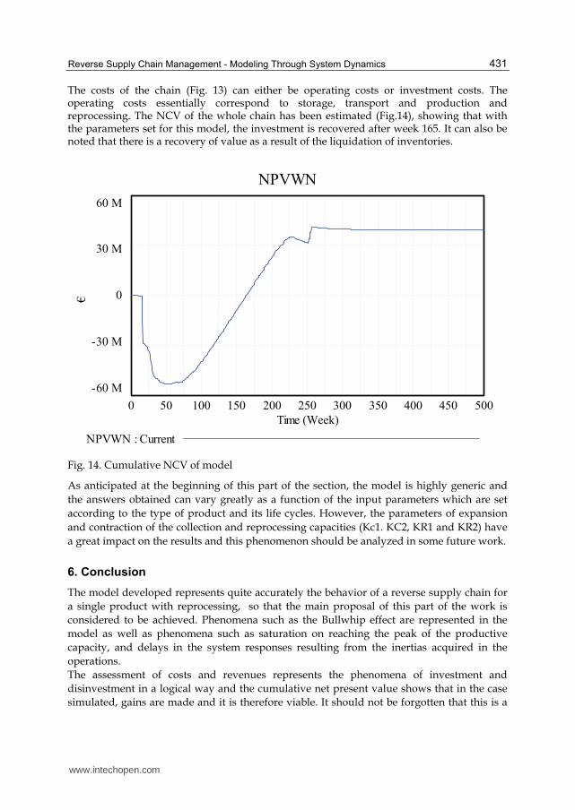
The costs of the chain (Fig. 13) can either be operating costs or investment costs. The operating costs essentially correspond to storage, transport and production and reprocessing. The NCV of the whole chain has been estimated (Fig.14), showing that with the parameters set for this model, the investment is recovered after week 165. It can also be noted that there is a recovery of value as a result of the liquidation of inventories.

NPVWN

60 M

30 M

0

-30 M

-60 M

0 50 100 150 200 250 300 350 400 450 500

Time (Week)

€

NPVWN : Current

Fig. 14. Cumulative NCV of model

As anticipated at the beginning of this part of the section, the model is highly generic and

the answers obtained can vary greatly as a function of the input parameters which are set

according to the type of product and its life cycles. However, the parameters of expansion

and contraction of the collection and reprocessing capacities (Kc1. KC2, KR1 and KR2) have

a great impact on the results and this phenomenon should be analyzed in some future work.

6. Conclusion

The model developed represents quite accurately the behavior of a reverse supply chain for

a single product with reprocessing, so that the main proposal of this part of the work is

considered to be achieved. Phenomena such as the Bullwhip effect are represented in the

model as well as phenomena such as saturation on reaching the peak of the productive

capacity, and delays in the system responses resulting from the inertias acquired in the

operations.

The assessment of costs and revenues represents the phenomena of investment and

disinvestment in a logical way and the cumulative net present value shows that in the case

simulated, gains are made and it is therefore viable. It should not be forgotten that this is a

www.intechopen.com


432

test case, a dummy, so that depending on the type of product that the model is applied to,

the economic results can vary significantly.

In short, we consider that modeling with system dynamics is an effective tool for describing reverse logistics systems due to the existence of delays and feedback loops. Moreover, system dynamics is a highly valuable and affordable method for performing simulations since all the variables and parameters are known; it is thus distinct form other simulation techniques that have more of a "black box" nature. Therefore we can conclude that it is a highly useful tool for decision-making.

7. Annex 1. Model variables

VARIABLE OR PARAMETER

SIGNIFICANCE OF VARIABLE OR PARAMETER

a-CC Parameter of delay in collection capacity

a-D Parameter delay in demand

a-DI Parameter of delay in distributors’ inventory

a-MI Parameter of delay in wholesalers’ inventory

a-RI Parameter of delay in retailers’ inventory

a-RPC Parameter of delay in reprocessing

a-RR Parameter of delay in reprocessing ratio

CCCCOST Costs of constructions for collection capacity

CCCR Ratio of contraction of collection capacity

CCDE Desired collection capacity

CCDI Discrepancy in collection capacity

CCER Ratio of expansion of collection capacity

CCIR Ratio of increase in collection capacity

CCOST Collection costs

CCRCOST Costs of reduction in collection capacity

CCRR Ratio of reduction in collection capacity

CCWCOST Weekly costs of collection capacity

CD Controlled disposal

CIC Coefficient of investment in collection

COR Collection capacity

CP Collected products

CR Collection ratio

CTCOST Costs of transport to clients

CWCOST Weekly costs of collection

www.intechopen.com


433



D Orders

DB Backorders

DCT Time of delivery to clients

DI Distributors’ inventory

DIAT Time of adjustment of distributors’ inventory

DICT Time of coverage of distributors’ inventory

DID Discrepancy with distributors’ inventory

DIDE Inventory of desired distributors

DIL Liquidation of distributors’ inventory

DILI Revenue from liquidation of distributors’ inventory

DILT Time of liquidation of distributors’ inventory

DISCOST Cost of storage of distributors’ inventory

DISWCOST Weekly cost of storage of distributors

DLP Distributors’ liquidation price

DO Distributors’ orders

DORR Ratio of reduction of backorders

DP Waste products

DST Time of delivery to distributors

DTCOST Cost of transport to distributors

DTWCOST Weekly cost of transport to distributors

ED Expected demand

EDO Orders expected from distributors

EMO Orders expected from wholesalers

ERO Orders expected from retailers

FP Percentage of error

ICOST Investment costs

ILI Revenue from liquidation of inventories

ILPI Revenue from liquidation of inventories of the plant

IT Inspection time

Kc1 Parameter of increase in collection capacity

Kc2 Parameter of reduction in collection capacity

Kr1 Parameter of increase in reprocessing capacity

www.intechopen.com


434



Kr2 Parameter of reduction in reprocessing capacity

LPP Liquidation price in plant

MBO Wholesalers’ Backorders

MFL Minimum for liquidation

MI Wholesalers’ inventory

MIAT Time of adjustment of wholesalers’ inventory

MICT Time of coverage of wholesalers’ inventory

MIDE Inventory of desired wholesalers

MIDI Discrepancy with wholesalers’ inventory

MIL Liquidation of wholesalers’ inventory

MILI Revenue from liquidation of wholesalers’ inventory

MILT Time of liquidation of wholesalers’ inventory

MISCOST Storage costs of wholesalers’ inventory

MISWCOST Weekly storage cost of wholesalers’ inventory

MLP Price of liquidation of retailers

MLPR Price of liquidation of wholesalers

MO Wholesalers’ orders

MOBRR Ratio of reduction in wholesalers’ backorders

MP Materials for processing

MS Deliveries to wholesalers

MSICOST Storage costs of retailers’ inventory

MSIWCOST Weekly storage costs of retailers’ inventory

MST Time of delivery to wholesalers

MTCOST Cost of transport to wholesalers

MTWCOST Weekly cost of transport to wholesalers

NCF Net cash flow

NPVP Current value of the period

NPVWN Current net value of the whole network

OB Backorders

OBRR Ratio of reduction of backorders

OCOST Operating costs

PARU Products accepted for reuse

www.intechopen.com


435



PC Production capacity

PCOST Production costs

PD Peak demand

PLIR Revenue from liquidation of retailers’ inventories

PR Production ratio

PRR Products rejected for reuse

PT Production Time

PTCOST Total costs per period

RCC Coefficient of reduction in collection

RCCCOST Costs of constructions for reprocessing capacity

RCCR Ratio of contraction in reprocessing capacity

RCDE Desired reprocessing capacity

RCER Ratio of expansion of reprocessing capacity

RCIR Ratio of increase in reprocessing capacity

RCRCOST Costs of reduction in reprocessing capacity

RCRR Ratio of reduction in reprocessing capacity

RCWCOST Weekly cost of reprocessing capacity

REP Reusable products

RER Expected reprocessing ratio

RI Retailers’ inventory

RIAT Time of adjustment to retailers’ inventory

RICOST Coefficient of investment in reprocessing

RICT Time of coverage of retailers’ inventory

RIDE Inventory of desired retailers’ inventory

RIDI Discrepancy with retailers’ inventory

RIL Liquidation of retailers’ inventory

RILT Time of liquidation of retailers’ inventory

RO Retailers’ orders

ROB Retailers’ backorders

ROBRR Ratio of reduction of retailers’ backorders

RPC Reprocessing capacity

RPCD Discrepancy with reprocessing capacity

www.intechopen.com


436



RPCOST Reprocessing costs

RPR Reprocessing ratio

RPSCOST Cost of storage of reusable products

RPT Reprocessing time

RRC Coefficient of reduction in reprocessing

RS Deliveries to retailers

RSKT Waiting time for reusable stock

RSPWCOST Weekly cost of storage of reusable products

RST Time of delivery to retailers

RT Time of residence

RTCOST Cost of transport to retailers

RTWCOST Weekly cost of transport to retailers

RWCOST Weekly cost of reprocessing

S Sales

SD Deliveries to distributors

SI Revenue from sales

SMPO Products sent to secondary markets

SP Sales price

STWCOST Weekly cost of sales transport

TIP Total revenue per period

Tc1 Time of increase in collection capacity

Tc2 Time of reduction in collection capacity

TPD Total demand pattern

Tr1 Time of increase in reprocessing capacity

Tr2 Time of reduction in reprocessing capacity

UD Uncontrolled disposal

UDP Products disposed of uncontrollably

UI Useful inventory

UIAT Time of adjustment to useful inventory

UICT Time of coverage of useful inventory

UID Discrepancy with useful inventory

UIDE Desired useful inventory

www.intechopen.com


437



UIL Liquidation of useful inventory

UILT Time of liquidation of useful inventory

UISCOST Cost of storage of useful inventory

UISWCOST Weekly cost of storage of useful inventory

UP Used products

WDR Weekly discount rate

WPCOST Weekly production costs

8. Annex 2. Model equations

Below are presented all of the equations that intervene in the model, numbered and ordered

alphabetically according to the name of the variables that describe them.

(001) "a-CC"= 12 Units: week Delay Parameter

(002) "a-D"= 2 Units: week Delay Parameter

(003) "a-DI"=2 Units: week Delay Parameter

(004) "a-MI"=2 Units: week Delay Parameter

(005) "a-RI"=2 Units: week Delay Parameter

(006) "a-RPC"=2 Units: week Delay Parameter

(007) "a-RR"=24 Units: week Delay Parameter

(008) CCCCOST=20000 Units: €/units

(009) CCCR=IF THEN ELSE(CCDE>lbc, MAX(-CCDI*Kc2, 0), COR) Units: units/week

(010) CCDE=SMOOTH(UP, "a-CC") Units: units/week

(011) CCDI=IF THEN ELSE(ABS(CCDE-COR)>lbc, CCDE-COR, 0) Units: units/week

(012) CCER=MAX(Kc1*CCDI, 0) Units: units/week

(013) CCIR=SMOOTH(CCER, Tc1) Units: (units/week)/week

(014) CCOST=5 Units: €/units

(015) CCRCOST= 5000 Units: €/units

(016) CCRR=CCCR/Tc2 Units: units/(week*week)

(017) CCWCOST= CIC*CCCCOST+RCC*CCRCOST Units: €/week

(018) CD=REP/RSKT Units: units/week

(019) CIC=CCER^0.6 Units: units/week

(020) COR= INTEG (CCIR-CCRR,0) Units: units/week

(021) CP= INTEG (CR-PARU-PRR,0) Units: units

(022) CR=MIN(COR, UP) Units: units/week

(023) CTCOST=1 Units: €/units

(024) CWCOST=CR*CCOST Units: €/week

(025) D=TPD(Time) Units: units/week

(026) DB= INTEG (D-DORR,0) Units: units

(027) DCT= 2 Units: week

(028) DI= INTEG (SD-MS-DIL,0) Units: units

www.intechopen.com


438

(029) DIAT= 1 Units: week

(030) DICT= 2 Units: week

(031) DID= MAX(DIDE-DI, 0) Units: units

(032) DIDE=EMO*DICT Units: units

(033) DIL=IF THEN ELSE(DIDE<MFL, DI/DILT, 0) Units: units/week

(034) DILI=DLP*DIL Units: €/week

(035) DILT=1 Units: week

(036) DISCOST=0.4 Units: €/(units*week)

(037) DISWCOST=DISCOST*DI Units: €/week

(038) DLP= 550 Units: €/units

(039) DO=EMO+DID/DIAT Units: units/week

(040) DORR=S Units: units/week

(041) DP= INTEG (CD+PRR,0) Units: units

(042) DST= 2 Units: week

(043) DTCOST=1 Units: €/units

(044) DTWCOST= DTCOST*SD Units: €/week

(045) ED=SMOOTH(D, "a-D") Units: units/week

(046) EDO= SMOOTH(DO, "a-DI") Units: units/week

(047) EMO= SMOOTH(MO, "a-MI") Units: units/week

(048) ERO= SMOOTH(RO, "a-RI") Units: units/week

(049) FINAL TIME=500 Units: week The final time for the simulation.

(050) FP=0.2 Units: Dmnl

(051) ICOST=CCWCOST+RCWCOST Units: €/week

(052) ILI=DILI+ILPI+MILI+PLIR Units: €/week

(053) ILPI=LPP*UIL Units: €/week

(054) INITIAL TIME=0 Units: week The initial time for the simulation.

(055) IT=1 Units: week

(056) k=1/(1+WDR)^Time Units: Dmnl Expression of discount rate for the net

current value (NCV). The discount rate is for a period of one week.

(057) Kc1=5 Units: Dmnl

(058) Kc2=1 Units: Dmnl

(059) Kr1=50 Units: Dmnl

(060) Kr2=1.8 Units: Dmnl

(061) lbc=0.05*PD Units: units/week

(062) lbr=0.05*PD Units: units/week

(063) LPP=550 Units: €/units

(064) MBO= INTEG (MO-MOBRR,0) Units: units

(065) MFL=10 Units: units

(066) MI= INTEG (MS-MIL-RS,0) Units: units

(067) MIAT=1 Units: week

(068) MICT=2 Units: week

(069) MIDE=ERO*MICT Units: units

(070) MIDI=MAX(MIDE-MI,0) Units: units

(071) MIL=IF THEN ELSE(MIDE<MFL, MI/MILT, 0) Units: units/week

www.intechopen.com


439

(072) MILI=MLPR*MIL Units: €/week

(073) MILT= 1 Units: week

(074) MISCOST=0.4 Units: €/units

(075) MISWCOST=MISCOST*MI Units: €/week

(076) MLP= 550 Units: €/units

(077) MLPR=550 Units: €/units

(078) MO=ERO+MIDI/MIAT Units: units/week

(079) MOBRR=MS Units: units/week

(080) MP= INTEG (-PR, 1e+007) Units: units

(081) MS=MAX( MIN(DI, MBO)/MST, 0) Units: units/week

(082) MSICOST=0.4 Units: €/units

(083) MSIWCOST=MSICOST*RI Units: €/week

(084) MST= 2 Units: week

(085) MTCOST=1 Units: €/units

(086) MTWCOST= MTCOST*MS Units: €/week

(087) NCF= (TIP-PTCOST)/(1+0.001) Units: €/week

(088) NPVP=NCF*k Units: €/week. The NCV is calculated for each period;

that is, in intervals of a week.

(089) NPVWN= INTEG (NPVP,0) Units: €. The NCV is calculated for the whole of

the supply chain.

(090) OB= INTEG (DO-OBRR,0) Units: units

(091) OBRR=SD Units: units/week

(092) OCOST= DISWCOST + UISWCOST + RSPWCOST + WPCOST + CWCOST +

RPWCOST + DTWCOST + STWCOST + RTWCOST + MSIWCOST + MISWCOST +

MTWCOST. Units: €/week

(093) PARU=CP*(1-FP)/IT Units: units/week

(094) PC=2000 Units: units/week

(095) PCOST=800 Units: €/units

(096) PD=1000 Units: units/week

(097) PLIR= MLP*RIL Units: €/week

(098) PR=MAX(MIN(PC, MIN( MP/PT, EDO-RER+UID/UIAT)), 0) Units: units/week

(099) PRR= CP*FP/IT Units: units/week

(100) PT=2 Units: week

(101) PTCOST=ICOST+OCOST Units: €/week

(102) RCC= CCRR^0.6 Units: units/week

(103) RCCCOST=120000 Units: €/units

(104) RCCR=IF THEN ELSE(RCDE>lbr, MAX(-RPCD*Kr2, 0), RPC) Units: units/week

(105) RCDE=SMOOTH(S*(1-FP), "a-RPC") Units: units/week

(106) RCER=MAX(Kr1*RPCD, 0) Units: units/week

(107) RCIR=SMOOTH(RCER, Tr1) Units: (units/week)/week

(108) RCRCOST= 40000 Units: €/units

(109) RCRR=RCCR/Tr2 Units: units/(week*week)

(110) RCWCOST= RICOST*RCCCOST+RRC*RCRCOST Units: €/week

(111) REP= INTEG (PARU-CD-RPR,0) Units: units

www.intechopen.com


440

(112) RER= SMOOTH(RPR, "a-RR") Units: units/week

(113) RI= INTEG (RS-RIL-S,0) Units: units

(114) RIAT= 1 Units: week

(115) RICOST=RCER^0.6 Units: units/week

(116) RICT= 2 Units: week

(117) RIDE=ED*RICT Units: units

(118) RIDI= MAX(RIDE-RI, 0) Units: units

(119) RIL=IF THEN ELSE(RIDE<MFL, RI/RILT, 0) Units: units/week

(120) RILT= 1 Units: week

(121) RO=ED+RIDI/RIAT Units: units/week

(122) ROB= INTEG (RO-ROBRR,0) Units: units

(123) ROBRR=RS Units: units/week

(124) RPC= INTEG (RCIR-RCRR,0) Units: units/week

(125) RPCD=IF THEN ELSE(ABS(RCDE-RPC)>lbr, RCDE-RPC, 0) Units: units/week

(126) RPCOST=25 Units: €/units

(127) RPR= MAX( MIN(REP/RPT, RPC), 0) Units: units/week

(128) RPSCOST= 0.4 Units: €/(week*units)

(129) RPT= 1 Units: week

(130) RPWCOST= RPR*RPCOST Units: €/week

(131) RRC= RCRR^0.6 Units: units/week

(132) RS=MAX( MIN(MI, ROB)/RST, 0) Units: units/week

(133) RSKT=4 Units: week

(134) RSPWCOST=REP*RPSCOST Units: €/week

(135) RST= 2 Units: week

(136) RT=RANDOM NORMAL(10, 30, 20, 2, 5) Units: week

(137) RTCOST=1 Units: €/units

(138) RTWCOST= RS*RTCOST Units: €/week

(139) S=MIN(DB, RI)/DCT Units: units/week

(140) SAVEPER = TIME STEP Units: week [0,?] The frequency with which output is

stored.

(141) SD=MAX( MIN(UI, OB)/DST, 0) Units: units/week

(142) SI=SP*S Units: €/week

(143) SMPO= INTEG (DIL+MIL+RIL+UIL,0) Units: units

(144) SP=1100 Units: €/units

(145) STWCOST=S*CTCOST Units: €/week

(146) Tc1= 8 Units: week

(147) Tc2= 8 Units: week

(148) TIME STEP = 1 Units: week [0,?] The time step for the simulation.

(149) TIP=SI+ILI Units: €/week

(150) TPD([(0,0)-(600,2000)],(0,0),(10,30),(20,100),(30,800),(40,900),(50,1000),(129,1000),

(130,1000),(180,1000),(181,1000),(200,1000),(210,900),(220,800),(230,100),(240,30),(250,0),(300,0)

,(500,0)) Units: units/week. Expected pattern of demand. Estimation according to the life

cycle of the various products.

(151) Tr1=24 Units: week

www.intechopen.com


441

(152) Tr2=8 Units: week

(153) UD=UP-CR Units: units/week

(154) UDP= INTEG (UD, 0) Units: units

(155) UI= INTEG (PR+RPR-SD-UIL,0) Units: units

(156) UIAT= 1 Units: week

(157) UICT= 2 Units: week

(158) UID=UIDE-UI Units: units

(159) UIDE=EDO*UICT Units: units

(160) UIL=IF THEN ELSE(UIDE<MFL, UI/UILT, 0) Units: units/week

(161) UILT= 1 Units: week

(162) UISCOST= 0.4 Units: €/(units*week)

(163) UISWCOST=UI*UISCOST Units: €/week

(164) UP=SMOOTH(S,RT) Units: units/week

(165) WDR=0.001 Units: Dmnl An annual discount rate of 5.2%

has been assumed, which means 0.1% per week.

(166) WPCOST=PCOST*PR Units: €/week

9. References

Fleischmann, M., Bloemhof-Ruwaard, J.M., Dekker, R. & van der Laan, E. 1997,

"Quantitative models for reverse logistics: A review", European Journal of Operational

Research, vol. 103, no. 1, pp. 1.

Fleischmann, M., Krikke, H.R., Dekker, R. & Flapper, S.D.P. 2000, "A characterisation of

logistics networks for product recovery", Omega, vol. 28, no. 6, pp. 653.

Forrester, J.W. 1961, Dinámica Industrial, "El Ateneo".

Georgiadis, P. & Vlachos, D. 2004, "The effect of environmental parameters on product

recovery", European Journal of Operational Research, vol. 157, no. 2, pp. 449-464.

Georgiadis, P., Vlachos, D. & Tagaras, G. 2006, "The Impact of Product Lifecycle on Capacity

Planning of Closed-Loop Supply Chains with Remanufacturing", Production and

Operations Management, vol. 15, no. 4, pp. 514.

Guide, V.D.R.,Jr & Srivastava, R. 1997, "Buffering from material recovery uncertainty in a

recoverable manufacturing environment", The Journal of the Operational Research

Society, vol. 48, no. 5, pp. 519.

Inderfurth, K., de Kok, A.G. & Flapper, S.D.P. 2001, "Product recovery in stochastic

remanufacturing systems with multiple reuse options", European Journal of

Operational Research, vol. 133, no. 1, pp. 130.

Jayaraman, V., Guide, V.D.R. & Srivastava, R. 1999, "A closed-loop logistics model for

remanufacturing", The Journal of the Operational Research Society, vol. 50, no. 5, pp.

497.

Kroon, L. & Vrijens, G. 1995, "Returnable containers: An example of reverse logistics",

International Journal of Physical Distribution & Logistics Management, vol. 25, no. 2, pp.

56.

Martín Garcia, J. 2003, Teoría y Ejercicios prácticos de Dinámica de Sistemas, ed. el autor.

www.intechopen.com


442

Mostard, J. & Teunter, R. 2006, "The newsboy problem with resalable returns: A single

period model and case study", European Journal of Operational Research, vol. 169, no.

1, pp. 81.

Pérez Ríos, J. 1992, Dirección Estratégica y Pensamiento Sistémico, Universidad de Valladolid.

Prahinski, C. & Kocabasoglu, C. 2006, "Empirical research opportunities in reverse supply

chains", Omega, vol. 34, no. 6, pp. 519-532.

Rogers, D. & Tibben-Lembke, R.S. 1999, Going Backwards: Reverse Logistics Trends and

Practices. Pittsburgh: RLEC Press.

Srivastava, S.K. 2007, "Green supply-chain management: A state-of-the-art literature

review", International Journal of Management Reviews, vol. 9, no. 1, pp. 53-80.

Sterman, J.D. 1989, "Modeling Managerial Behavior: Misperceptions Of Feedback In",

Management Science, vol. 35, no. 3, pp. 321.

Vlachos, D., Georgiadis, P. & Iakovou, E. 2007, "A system dynamics model for dynamic

capacity planning of remanufacturing in closed-loop supply chains", Computers &

Operations Research, vol. 34, no. 2, pp. 367-394.

www.intechopen.com

Supply Chain Management - New PerspectivesEdited by Prof. Sanda Renko

ISBN 978-953-307-633-1Hard cover, 770 pagesPublisher InTechPublished online 29, August, 2011Published in print edition August, 2011

InTech EuropeUniversity Campus STeP Ri Slavka Krautzeka 83/A 51000 Rijeka, Croatia Phone: +385 (51) 770 447 Fax: +385 (51) 686 166www.intechopen.com

InTech ChinaUnit 405, Office Block, Hotel Equatorial Shanghai No.65, Yan An Road (West), Shanghai, 200040, China

Phone: +86-21-62489820 Fax: +86-21-62489821

Over the past few decades the rapid spread of information and knowledge, the increasing expectations ofcustomers and stakeholders, intensified competition, and searching for superior performance and low costs atthe same time have made supply chain a critical management area. Since supply chain is the network oforganizations that are involved in moving materials, documents and information through on their journey frominitial suppliers to final customers, it encompasses a number of key flows: physical flow of materials, flows ofinformation, and tangible and intangible resources which enable supply chain members to operate effectively.This book gives an up-to-date view of supply chain, emphasizing current trends and developments in the areaof supply chain management.

How to referenceIn order to correctly reference this scholarly work, feel free to copy and paste the following:

Rafael Rodriguez-Ferna ndez, Beatriz Blanco, Adolfo Blanco and Carlos A. Perez-Labajos (2011). ReverseSupply Chain Management – Modeling Through System Dynamics, Supply Chain Management - NewPerspectives, Prof. Sanda Renko (Ed.), ISBN: 978-953-307-633-1, InTech, Available from:http://www.intechopen.com/books/supply-chain-management-new-perspectives/reverse-supply-chain-management-modeling-through-system-dynamics

© 2011 The Author(s). Licensee IntechOpen. This chapter is distributedunder the terms of the Creative Commons Attribution-NonCommercial-ShareAlike-3.0 License, which permits use, distribution and reproduction fornon-commercial purposes, provided the original is properly cited andderivative works building on this content are distributed under the samelicense.

https://creativecommons.org/licenses/by-nc-sa/3.0/

Documents

Reverse Supply Chain Management - Modeling Through …cdn.intechopen.com/pdfs/18519/InTech-Reverse_supply_chain_management... · 20 Reverse Supply Chain Management - Modeling Through