1

Lunds Universitet Ekonomihögskolan Företagsekonomiska Institutionen

FEKH89 Examensarbete i Finansiering på Kandidatnivå

HT 2013

Reverse Mergers - An Alternative to IPOs – A study of reverse merger long-term performance

Författare: Gabriel Hahn

Lennart Lindrud Amra Ramić Handledare:

Tore Eriksson

Grupp: 6

2

Abstract Title: Reverse Mergers - An Alternative to IPOs Seminar date: 2014-01-17 Course: FEKH89 Finance: Degree Project Undergraduate level, 15 ECTS Authors: Gabriel Hahn, Lennart Lindrud, Amra Ramic Advisor: Tore Eriksson Key words: Reverse mergers, Reverse takeovers, IPO, BHAR, HPR, t-tests,

confidence interval. Purpose: The aim of this study is to determine whether reverse mergers are

a viable alternative to IPOs in going public. This is done by measuring buy-and-hold abnormal returns (BHAR) for each group and comparing them for a three year period. Furthermore, we look at factors that might explain discrepancies.

Methodology: We have carried out a long-term event study with a deductive approach. Our empirical material is mainly made up of secondary data, which we analyze using the buy-and-hold abnormal returns method. The data is then tested via t-tests and confidence intervals.

Theoretical perspective: This research is based on previous studies done on IPOs and

reverse mergers from all around the world, but mostly USA. Empirical foundation: Our research is based on data from companies on the Swedish

stock exchanges. The data was obtained from Thomson Reuters Datastream as well as from Skatteverkets webpage.

Conclusions: We find no significant difference in RM and IPO performance in

terms of BHARs. Therefore, RMs are a viable option and they should be considered a legitimate alternate means of going public, despite the bad reputation.

3

Abstract Titel: Reverse Mergers - An Alternative to IPOs Seminarie datum: 2014-01-17 Kurs: FEKH89 Finance: Degree Project Undergraduate level, 15 ECTS Författare: Gabriel Hahn, Lennart Lindrud, Amra Ramic Handledare: Tore Eriksson Nyckelord: Reverse mergers, Reverse takeovers, IPO, BHAR, HPR, t-tests,

confidence interval. Syfte: Syftet med denna studie är att utreda huruvida omvända förvärv är

ett hållbart alternativ till att bli börsnoterat jämfört med IPOs. Detta görs genom att mäta överavkastning för båda grupperna på tre års sikt och sedan jämföra dem med varandra. Dessutom undersöks faktorer som kan förklara eventuella diskrepanser.

Metod: En eventstudie med deduktiv ansats har utförts, där vi analyserar

det empiriska materialet med hjälp av BHAR metoden. Empirin är sedan testad via t-test och konfidens intervaller.

Teori: Denna studie bygger på tidigare forskning som gjorts på IPOs samt

omvända förvärv runtom i världen. Det mesta är dock baserat på studier i USA.

Empiri: Vårt arbete baseras på data av företag noterade på Svenska börser

och handelsplattformar. Den empiriska datan insamlades via Thomson Reuters Datastream funktion samt från Skatteverkets hemsida.

Slutsatser: Ingen signifikant skillnad påvisades mellan omvända förvärv och

IPO företagens överavkastning. Vi drar slutsatsen att omvända förvärv är ett legitimt alternativ till att ta sig in på börsen, trots det dåliga ryktet.

4

Table of Contents 1 Introduction ........................................................................................................................................ 6

1.1 Background .................................................................................................................................. 6

1.2 Problem Discussion ..................................................................................................................... 9

1.3 Purpose ....................................................................................................................................... 11

1.4 Target Group ............................................................................................................................. 11

1.5 Demarcations ............................................................................................................................. 11

2 Literature Study ............................................................................................................................... 12

2.1 Stock Exchange .......................................................................................................................... 12

2.2 Initial Public Offerings (IPO) ................................................................................................... 13

2.3 Reverse Mergers, a Comparison .............................................................................................. 14

2.3.1 Advantages vs. IPOs ........................................................................................................... 15

2.3.2 Disadvantages vs. IPOs ...................................................................................................... 16

2.4 Shell Companies ........................................................................................................................ 17

3 Earlier Research in Regards to Methodology ................................................................................ 18

3.1 BHAR ......................................................................................................................................... 18

3.2 Cumulative Abnormal Return (CAR) ..................................................................................... 20

4 Methodology ..................................................................................................................................... 22

4.1 Quantitative Research Method ................................................................................................ 22

4.1.2 Gathering of Data ............................................................................................................... 22

4.1.3 Data selection ...................................................................................................................... 23

4.2 Reliability ................................................................................................................................... 24

4.3 Validity ....................................................................................................................................... 24

4.4 Buy and Hold Abnormal Returns ............................................................................................ 24

4.4.1 Matching Concept .............................................................................................................. 25

4.5 The t-test and Confidence Intervals ......................................................................................... 26

4.6 Hypothesis Testing .................................................................................................................... 27

5 Analysis and Results ......................................................................................................................... 29

5.1 Observation trends .................................................................................................................... 29

5.4 Connecting the Dots, Comparison to Previous Studies .......................................................... 40

5.5 Critique and Limitations .......................................................................................................... 43

6 Conclusion ......................................................................................................................................... 44

6.1 Suggestions for further research .............................................................................................. 45

5

7 Bibliography ..................................................................................................................................... 46

7.1 Articles ........................................................................................................................................ 46

7.2 Literary sources ......................................................................................................................... 47

7.3 Digital sources ............................................................................................................................ 48

7.4 Databases .................................................................................................................................... 49

8 Appendices ........................................................................................................................................ 50

6

1 Introduction

1.1 Background The year of 2008 will long be remembered as the year that triggered chaos, with crashing

stock markets, huge bankruptcies and bailouts around the world. Books are, and continue to

be written about the cause and effects of that crash. While stockowners experienced a

harrowing journey, firms also suffered, in particular the ones in need of capital injections. The

ones seeking to go public via an initial public offering (IPO) found that the market had

completely dried up. The capital markets were at a standstill and would continue to be for

years. In 2008, over 100 companies cancelled their IPO plans in USA alone (Feldman, 2009).

What were their options?

Fast forward to December 2013, and zoom in to a small Scandinavian nation; Sweden. A

Swedish company by the name of Candyking had planned to undertake an IPO on the

Swedish stock market (Nasdaq OMX). According to the company, there had been a growing

interest among investors to participate. However, the day before the planned IPO Candyking

sent out a press release informing the public that two fires had broken out in their supplier’s

factories. Profits would be SEK 3.5 million lower than previously forecasted. The offering

was to be delayed a few days for that reason. However, disclosing negative news at this

crucial stage in the process was enough to scare many investors away, and eventually, due to

negative press, Candyking thought better of it and aborted the offering completely.

Obviously, the release of bad news was ill-timed, but with 2012 revenues at SEK 1.8 billion,

the SEK 3.5 million was a drop in the bucket and should not have affected the long-term

valuation of the company much. In fact, Candyking stated that “even with these negative

effects during the fourth quarter, the company expects a higher underlying operating profit in

2013 than 2012” (Placera, 2008). So why did Candyking choose to abort their IPO? We

venture to guess that perhaps they would not have received the amount they sought, or the

valuation they wanted. Regardless, they were at the mercy of external forces.

This chapter provides background information on the subject and explains our problem formulation in regards to earlier research.

7

So what is the lesson here? IPOs have some apparent flaws, certainly with regards to factors

outside the companies’ control like bull/bear markets and investor irrationality. When

recessions occur and the IPO market shuts down, alternate routes for going public are needed.

Furthermore, firms would prefer those routes to be less sensitive to irrational behavior due to

short-term problems.

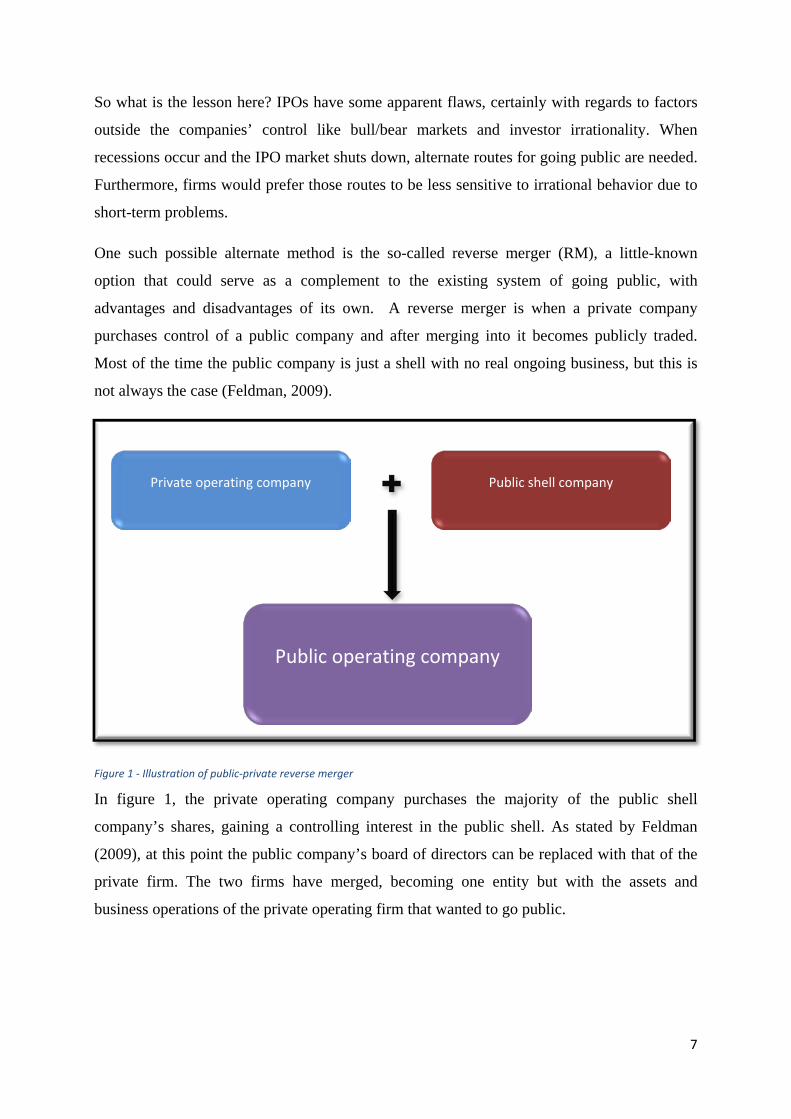
One such possible alternate method is the so-called reverse merger (RM), a little-known

option that could serve as a complement to the existing system of going public, with

advantages and disadvantages of its own. A reverse merger is when a private company

purchases control of a public company and after merging into it becomes publicly traded.

Most of the time the public company is just a shell with no real ongoing business, but this is

not always the case (Feldman, 2009).

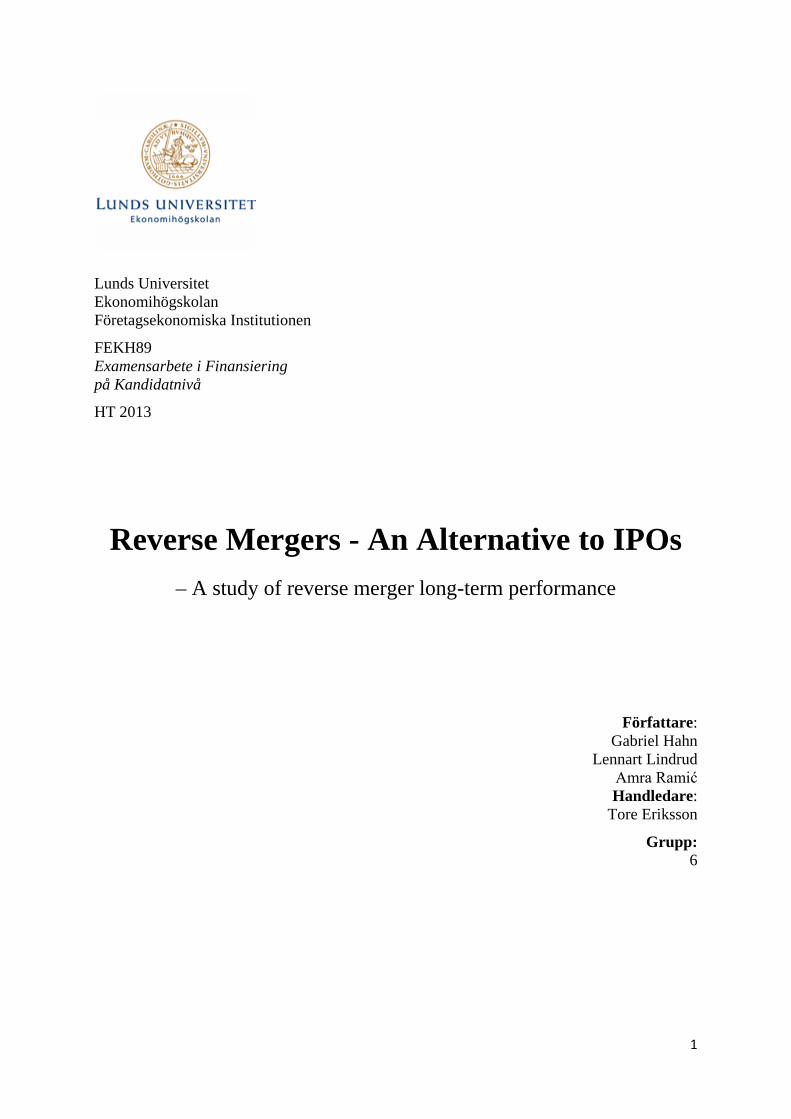
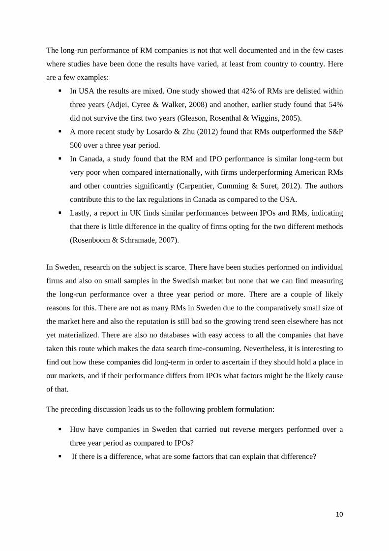
In figure 1, the private operating company purchases the majority of the public shell

company’s shares, gaining a controlling interest in the public shell. As stated by Feldman

(2009), at this point the public company’s board of directors can be replaced with that of the

private firm. The two firms have merged, becoming one entity but with the assets and

business operations of the private operating firm that wanted to go public.

Private operating company Public shell company

Public operating company

Figure 1 - Illustration of public-private reverse merger

8

Although the RM method is not well known, it might surprise the reader to know that some

very large and profitable companies have used it, including the following (Feldman 2009):

• Berkshire Hathaway Inc

• Jamba Juice, Inc

• Texas Instruments Inc

• Blockbuster Entertainment

• The New York Stock Exchange

• Radio Shack (Tandy Corporation)

If respectable firms like these used it, it may be worthwhile inspecting the method closer.

Unfortunately, RMs have long had a bad reputation due to the prevalence of fraud involved in

deals made in the past, especially in the 80s in USA. This was mostly done through shell

companies that went public with the sole purpose of raising money, which they then used to

pay themselves salaries and fees, with no real business going on. In USA, the stigma has

started to decrease, leading to a surge in the number of RMs undertaken since 2000 (Feldman

2009). Feldman mentions several possible reasons for this change:

IPOs have been hard to undertake since 2000, so alternate methods are sought

Since 2004, a new group of investors have discovered reverse mergers, so called PIPE

investors (Private Investment in Public Equity). These investors refer to it as “public

venture capital”.

The SEC and financial community have begun to see reverse mergers as a legitimate

way to go public.

Of the 39 companies we found that have gone public through a reverse merger in Sweden

between 2000 and 2010, almost 25% have gone bankrupt or been delisted. A simple Google

search on reverse mergers will reveal how negative the public opinion is in Sweden. The title

of an article written in Aktiespararen 2011 perhaps sums up the public view of investors,

“Omvänt förvärv banar vägen för bedragarna” which translates to “Reverse mergers pave the

way for fraudsters” (Bernholm, 2011). The harsh critique is justified in that particular article,

but how often is that the case? Is the negative view warranted or is the RM option a viable

one?

9

1.2 Problem Discussion Much has been written on IPOs regarding the characteristics of companies that choose this

route, as well as their subsequent performance on the market. Research on the subject has

often focused on the four puzzles of IPOs: short-run underpricing, long-run

underperformance, high costs and the wave-like pattern of IPOs.

For example, Ibbotson, Sindelar, and Ritter (1994) found that IPOs around the world tend to

follow economic patterns, with many being undertaken during good times and few being

undertaken during downturns. Interestingly, RMs are not as sensitive to market fluctuations as

IPOs, aside from extreme events such as the financial crisis in 2008. That makes them a

viable option in bad markets, but does not necessarily limit them to those situations. A study

in USA comparing RMs and IPOs found that there is a negative correlation between the two

in terms of number of deals occurring per year (Losardo & Zhu, 2012). This implies that

firms do in fact sometimes use RMs as a substitute for IPOs.

The long-run underperformance puzzle of IPOs mentioned above is interesting from an

investor’s point of view and is documented by Ritter in 1998. He found that IPOs appeared to

be overpriced, which lead to long-run underperformance of stock returns as the price

eventually corrects itself. Another theory presented is that the IPO itself is not important;

instead the reason for going public is what drives the long-term negative performance.

While IPOs continue to be the most common way to go public, the number of RMs is rising,

especially after 2000 (Feldman, 2009). So why are RMs important, aside from their growing

popularity? There are a number of reasons, according to Feldman. Many small companies

could benefit from being publicly listed but cannot undertake an IPO, partly because they do

not live up to the high-growth standards that investment companies often seek and partly

because the fees are exorbitant. RMs are cheaper because they do not require expensive

underwriters and the process of going public is quicker because it does not go through the

same regulation processes. The disadvantages are that there is less funding and the shares are

not traded frequently. The details of RMs will become clear later in this report. For now,

suffice it to say that the method is interesting to investigate further, specifically in regards to

how these companies perform as compared to IPO companies.

10

The long-run performance of RM companies is not that well documented and in the few cases

where studies have been done the results have varied, at least from country to country. Here

are a few examples:

In USA the results are mixed. One study showed that 42% of RMs are delisted within

three years (Adjei, Cyree & Walker, 2008) and another, earlier study found that 54%

did not survive the first two years (Gleason, Rosenthal & Wiggins, 2005).

A more recent study by Losardo & Zhu (2012) found that RMs outperformed the S&P

500 over a three year period.

In Canada, a study found that the RM and IPO performance is similar long-term but

very poor when compared internationally, with firms underperforming American RMs

and other countries significantly (Carpentier, Cumming & Suret, 2012). The authors

contribute this to the lax regulations in Canada as compared to the USA.

Lastly, a report in UK finds similar performances between IPOs and RMs, indicating

that there is little difference in the quality of firms opting for the two different methods

(Rosenboom & Schramade, 2007).

In Sweden, research on the subject is scarce. There have been studies performed on individual

firms and also on small samples in the Swedish market but none that we can find measuring

the long-run performance over a three year period or more. There are a couple of likely

reasons for this. There are not as many RMs in Sweden due to the comparatively small size of

the market here and also the reputation is still bad so the growing trend seen elsewhere has not

yet materialized. There are also no databases with easy access to all the companies that have

taken this route which makes the data search time-consuming. Nevertheless, it is interesting to

find out how these companies did long-term in order to ascertain if they should hold a place in

our markets, and if their performance differs from IPOs what factors might be the likely cause

of that.

The preceding discussion leads us to the following problem formulation:

How have companies in Sweden that carried out reverse mergers performed over a

three year period as compared to IPOs?

If there is a difference, what are some factors that can explain that difference?

11

1.3 Purpose The purpose of this study is to determine whether RMs are a viable alternative to IPOs in

going public. This is done by measuring buy-and-hold abnormal returns (BHAR) for each

group and comparing them during a three year period. Furthermore, we look at factors that

might explain discrepancies.

1.4 Target Group The target group for this paper is mainly people with a basic knowledge of business,

economics, or finance. These include teachers, students, professors; and possibly investors

seeking an investment strategy. Furthermore, we hope to provide firms with information on an

otherwise obscure method of going public.

1.5 Demarcations This paper will examine and compare Swedish companies that have undertaken RMs and

IPOs in the time span 2000 to 2010. We see a time period of 10 years as a sufficient time to

examine this subject as this time span should include a whole business cycle which is usually

three to eight years (Konjunkturterminologi, 2011).

We wish to examine the long-run performance for three years, which means the latest starting

date that can be used is 2010 (the study starts in 2013). This study is limited to using BHAR

when measuring the long-run returns which has been deemed to be an adequate measure when

determining the viability of the firms. The study is limited to adjusted stock returns (which

adjusts for capital events). Additionally, we only use companies registered on the stock

markets NGM, Aktietorget, NASDAQ OMX, and First North.

12

2 Literature Study

2.1 Stock Exchange The type of stock exchange a company chooses to go public on says a good deal about a

company. Smaller stock exchanges such as Nordic Growth Market (NGM) Equity and

Aktietorget attract smaller, more growth-oriented firms that are in need of capital in order to

keep expanding and developing. There are a number of listing requirements for each stock

exchange. On the NGM stock exchange you are required to have at least 300 stock owners

where each stock owner has shares valued at a minimum of 5000 SEK, and where at least

10% of the votes and 10% of the stocks are spread amongst the public (NGM, 2013).

However, as NGM is one of the two regulated market places in Sweden it has stricter listing

requirements than Aktietorget and First North.

NASDAQ OMX is the other regulated market place, and has the strictest requirements for

listing companies. Firms have to prepare a prospectus that must be approved by relevant

authorities. Furthermore, the company must undergo legal examination that covers several

areas. There are fees that must be covered and proofs of profitability over a certain amount of

years must be provided. These are some of the requirements companies must fulfill before

listing. Further details can be found on the NASDAQ OMX official website. The main thing

we want to highlight is that NASDAQ OMX is the strictest exchange to list on, and is aimed

at companies that are stable and can show a profitable past. Even if a company fulfills the

requirements, NASDAQ OMX retains the right to decline a company’s listing application if it

can be deemed to harm the credibility of the stock exchange (NASDAQ OMX Rulebook,

2014). For future reference, note that we use NASDAQ OMX and Nordiska interchangeably

in the rest of this paper.

Aktietorget exists to aid young growth companies in gaining access to investor capital from

the public. Aktietorget changed on the 29th of March 2007, it is no longer a regulated market

in the sense that NASDAQ OMX and NGM are. The general listing requirements of

Aktietorget are that there has to be at least 200 shareholders holding shares with a value of

In this chapter we will present and discuss theories and practical information that is relevant to our subject. We discuss the different stock exchanges, IPO puzzles, and RM characteristics.

13

circa SEK 4,400 each. Aktietorget has chosen to enlist an external disciplinary committee and

has organized market surveillance even though it is not required, “in order to resemble a

regulated market” (Aktietorget, 2014).

First North is NASDAQ OMX’s growth market, specifically for smaller, developing

companies. It does not have the same regulations that are set on other markets but is regulated

by the rules set forth by First North; a company on First North is considered to be a more

risky investment than companies on the regulated markets mentioned above. However, an

added benefit of less stringent rules is that it allows for the listed companies to be freer in

their development and more focused on their own activities. The general listing requirements

are that a company must have a “sufficient amount of shareholders holding shares with a

value of at least 500 EUR and if at least 10% of the share class to be traded is held by the

general public” (First North Nordic – Rulebook, 2013).. Furthermore, a company must fulfill

the company description, sign an agreement with a certified adviser, and must meet the

organizational requirements (First North Nordic – Rulebook, 2013).

Before moving on we want to emphasize that the actual rules for each market aren’t that

important in our analysis, rather it is the differences between them that we are interested in

due to the possible effect that might have on long-run performance.

2.2 Initial Public Offerings (IPO)

Through an initial public offering a private company can become a public one as the shares of

a company are sold out to the general public and traded on the stock markets. Public offerings

thereafter are called seasoned equity offerings, or SEOs. IPOs are often made by small

companies that need new capital to be able to expand or grow.

Advantages of going public are, among other things: greater liquidity, easier access to capital,

public awareness of the company, and the spreading of risk for the owners. However, there

are some disadvantages as well. Finansinspektionen (FI) requires all publicly traded

companies to publish all information that could have an influence on the quotation of the

stock (ÅRL, 1995:1554). Additionally, accurate financial statement reports need to be

released regularly, a process that takes time and is costly due to audit fees.

14

There are four main problems with going through an initial public offering, often referred to

as the “four IPO puzzles” (Berk & DeMarzo, 2013).

1. IPOs are underpriced in the short term; they have on average had positive abnormal

returns the first day the stock is sold, and has been observed all around the world. It is

often young firms that go through with an IPO. It is very uncertain how their business

will develop and this uncertainty won’t attract risk averse investors unless the share is

underpriced (Rock, 1986).

2. New issues are highly cyclical, with more deals done in bull markets. It is pretty

obvious that there would be a higher need for capital when there are more growth

opportunities; the surprising part is the extent of the difference (Ritter, 2011).

3. IPOs are expensive, with both direct and indirect costs. Chen & Ritter (2000) found

that for IPOs, the direct costs average 11%. On top of that there are indirect costs

associated with underpricing by the underwriters.

4. The long-run performance (3-5 years) after an IPO is on average poor. The theory of

adverse selection suggests that “bad” products are bought because of asymmetric

information. Ritter (1991) attributes the long-run underperformance mostly to market

timing, where certain industries are doing well and so many companies in that sector

go public during that time. Then the price is corrected with time. Another theory is

that the reasons behind the IPO are what matters most.

2.3 Reverse Mergers, a Comparison In this section we will explain what a reverse merger is, why it might be beneficial for some

firms and what circumstances warrant its use, as well as what constitutes a shell company in

the RM process.

In his book, Reverse Mergers, David Feldman (2009) describes the reverse merger process

in-depth and explains why it is a viable option for small firms. Much of the material in this

section is taken from his book. Surprisingly, this is one of the only books written on the

subject and although it is aimed at an American audience it is nevertheless relevant even to

15

the Swedish market, as the process is similar. Differences between the two are mainly found

in regulatory requirements and legislation. These are not trivial and as stated previously have

been found to have a significant effect on long term performance of newly listed firms

(Carpentier, Cumming & Suret, 2012). In our study however, we only compare Swedish

companies to each other so the differences are irrelevant in this particular case.

A reverse merger is when “a private company purchases control of a public one, merges into

it, and when the merger is complete becomes a publicly traded company in its own right”

(Feldman, 2009). If the public company has no real ongoing business then it is often referred

to as a “shell”. The reasons for going public this way will become apparent as we go through

the advantages and disadvantages below. Feldman names seven advantages and two

disadvantages of RMs when compared to IPOs. We cover each briefly.

2.3.1 Advantages vs. IPOs 1. Lower cost.

One of the puzzles of IPOs is the high underwriting costs (Ritter, 1991). This is

avoided in the RM process. Feldman states that RMs are much less costly and the total

cost can often be pre-determined. In his experience, most RMs cost less than $1

million whereas an IPO will cost at least three or four times that much, excluding

underwriting commissions (2009). For a RM the biggest cost is generally the price of

the shell.

2. Speedier Process

A RM takes two to three months; an IPO takes nine to twelve. There are fewer steps

and fewer parties involved. There is also no disclosure document that needs to be

approved by the SEC.

3. Not Dependent on IPO Market for Success

As discussed earlier, IPOs follow a wave-like pattern and prefer to go public when the

economy is doing well (Ritter, 1984). This is not an issue for RMs, because they are

not sensitive to the market and that makes them a good choice in any market

condition.

16

4. Not Susceptible to Changes from Underwriters Regarding Initial Stock Price

Underwriters can choose to change the price at the last minute if the market sentiment

drops just before the IPO. Cancellations of IPOs are also not uncommon.

5. Less Time-Consuming for Company Executives

IPOs take time, time that could be used to run the business. A RM is less time-

consuming as mentioned earlier and no new investors need to be found. That means

more time for business decisions.

6. Less Dilution

Feldman argues that in a RM less money is raised, during a time when the company

supposedly is undervalued. It is better to raise money when the stock price is higher,

because it doesn’t dilute ownership. Theoretically, new companies on the public

market should trade higher after six months or so if the business grows. That is a big

“if” however. Additionally, underwriters tend to try to take in as much money as

possible without regard to how much the company doing the IPO actually needs (what

you might call a “good” problem). This is because the underwriter takes a percentage

fee of what is raised.

7. Underwriters Unnecessary

Feldman mentions this one because underwriters try to make a company look as

profitable as possible before the IPO, which sometimes means selling off new

subsidiaries that have not yet started making money. RMs do not have that problem as

there are no underwriters involved.

2.3.2 Disadvantages vs. IPOs 1. Less Funding

RMs bring in less money than an IPOs but that may not be relevant criticism of the

method. Nothing stops the company from taking in new capital once they are public.

This may even be beneficial if the stock price is higher at that point.

17

2. Market Support is Harder to Obtain

Underwriters will for some time after the IPO of a firm act as market makers, as well

as trying to hype the stock during and after the offering. This often results in what

Feldman calls a “pop in the stock price” which is unlikely in a RM because no one is

covering the stock. A rise is more likely to come from years of improved performance

rather than what he calls “manufactured support”.

To sum up, the main situations in which RMs are preferable to IPOs is when firms are small,

markets are down, initial injection of money is not the main aim, time is of importance, or

simply when hefty fees wish to be avoided. These are definitely compelling reasons to

perform RMs.

2.4 Shell Companies The target firms of RM deals are typically unprofitable, so-called shell companies. A shell

company is a company registered with the FI (Finansinspektionen – equivalent to the U.S

Security and Exchange Commission) and is overall emptied of its real assets. If these add up

to at least half of the disposal price the company is classified by Sweden’s government

(Proposition 2001/02:165) as a shell company. Shell companies typically trade on smaller

markets. A shell company might have been founded simply for the purpose of merging with

other companies or because they might have been forced to sell off all their assets due to

bankruptcy. Shell companies are not the focus of this study so no detailed description is

needed but in certain studies a distinction is made between deals involving shells and others

that are more strategic in nature, like mergers. We do not make that distinction here.

18

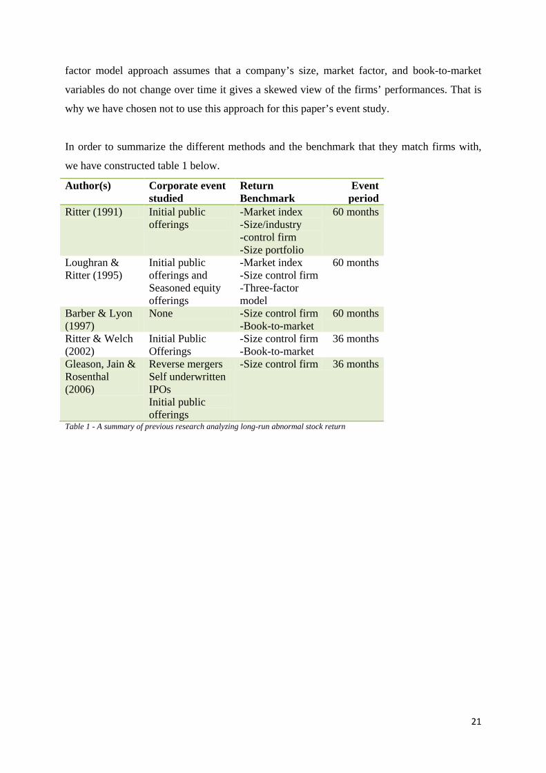
3 Earlier Research in Regards to Methodology

The calculation of abnormal returns in order to gauge a stock’s performance in a post-event

window has been common over the past two decades, as table 1 illustrates. Mainly, these

event studies have been performed on corporate events such as IPOs and Seasoned Equity

Offerings (SEO). There are three commonly used methods of measuring stock returns,

namely: BHAR, CAR, and the Fama-French three factor model, all of which will be

discussed.

3.1 BHAR A study by Gleason, Jain & Rosenthal (2006) is one of the few that utilize a quantitative

approach to analyze the long-run performance of RMs vs IPOs. They collected data that

included 119 confirmed RMs and 22 self-underwritten (SU) IPOs listed on the New York,

NASDAQ, or American stock exchanges between 1986 and 2003. They then gathered sample

IPOs that would act as matching companies, and these were value weighted, meaning that the

category they matched IPOs, RMs, and SUs by was the firm’s market capitalization at the

time of the RM or SU event. They research the long-run market value performance by

calculating buy-and-hold returns for the RMs and SU for 6, 12, 18, 24, and 36 months. The

buy-and-hold abnormal return (BHAR) was then calculated as the difference between the

sample RM or SU firm holding period (HPR) and the HPR for the matching IPO firm. By

doing this, Gleason, Jain & Rosenthal (2006) analyze the long-run returns of the private

company that undertakes a RM to go public from a shareholder’s perspective, and by using

the matching principle the authors identify whether or not the shareholder would have been

better off investing in a traditional IPO.

They tested the significance of the mean and median using t-tests and Wilcoxon Signed Rank

tests at the 1, 5, and 10% levels. The researchers found that the long-run performance of RMs

outperform their matched traditional IPO firm in the short-run and performed similarly in

three years after going public. The researchers conclude that this may not be all that surprising

due to the fact that so many RMs and SUs were undertaken during the dot-com bubble.

In this chapter we will highlight and discuss earlier research methods that are applicable to this study, as well as motivating why we chose the one used in this paper.

19

However, what is interesting is that from an investor perspective one would not have

underperformed if investing in a RM during the study’s time period.

Loughran & Ritter (1995) used a sample of 4,735 companies going public (IPO) in the United

States between 1970 and 1990. They calculated the BHAR annually for 5 years starting from

the first year after the event date. They then use a matching firm for each issuing company

and match them by market capitalization. The firm with the closest to but higher market

capitalization is chosen as a matching firm for the issuing company. If one of the matching

firms delisted, Loughran and Ritter (1995) chose to switch over to a second matching firm on

the date it was delisted. By doing this they manage to remove survivorship bias. The authors

argue that matching by industry as well as market capitalization would not be possible due to

the fact that there would not be enough firms and they would have to re-use the same

matching firms. They found when looking at the 3 year BHAR mean of the IPO and the

matching firm that the IPOs underperformed; which matches what earlier studies such as

Ritter (1991) concluded on the subject. When looking at a 5 year BHAR mean the IPOs

underperformed even more. Loughran & Ritter (1995) conclude that IPOs during this time

period have been poor long-run investments for investors.

Ritter & Welch (2002) research a sample of 6,249 IPOs in the time period 1980 to 2001. They

tested the long-run performance in order to determine if the theory of long-run

underperformance is valid. They do this by testing the IPOs BHAR relative to a benchmark

and use a value-weighted portfolio as the benchmark, as well as matching the IPOs to control

firms, testing both methods. They found that the BHAR mean for IPOs when matched with

the portfolio was -23.4% from 1980-2001 whereas when the IPOs were matched with the

control firm the BHAR mean was -5.1% which shows a big difference in performances.

However, both methods resulted in IPOs underperforming in 3 years.

Barber & Lyon (1997) argue that event studies should calculate abnormal returns by using the

simple buy-and-hold return on a sample firm minus the simple buy-and-hold return on a

reference portfolio or a matching firm. They identify three biases: new listing, rebalancing,

and the skewness bias and explain how to remove these biases. We will go through how the

biases are removed in section 4.4.1. The use of a control/matching firm by size and book-to-

market ratios result in more efficient test statistics in all different kinds of scenarios that

Barber & Lyon (1997) can imagine. They argued that the control/matching firm method

20

results in more efficient test statistics than a reference portfolio because it reduces the three

biases. Their data showed that when using the control/matching firm the mean BHAR and

bias’ are overall much closer 0 than when the reference portfolio is used.

3.2 Cumulative Abnormal Return (CAR) An alternative to the use of BHAR would be the cumulative abnormal return (CAR). Barber

& Lyon (1997) argue that summing daily or monthly abnormal returns introduces bias in the

event study as well as positively biased test statistics due to the three biases mentioned earlier.

Ritter (1991) was among the first researchers to argue that CAR and BHAR can be used in

order to answer different types of questions. The difference between the two methods is that

CAR disregards the effect of monthly compounding whereas BHAR includes it. Barber &

Lyon (1997) test this by randomly sampling 10,000 firms between July 1963 and December

1993. Then the 12-month CAR and BHAR is calculated using the CRSP

NYSE/NASDAQ/AMEX equally weighted market index for each of the 10,000 samples

which were then sorted into 100 portfolios of 100 samples each. Additionally, they calculate

the mean difference between the CAR and BHAR and then test the difference against the

mean annual BHAR of each of the 100 portfolios. This showed the differences between CAR

and BHAR, and when the annual BHAR was less than 13%, the CAR was on average almost

5% greater than the BHAR. However, as the BHAR increased, the CAR decreased

significantly. This difference was a result of monthly compounding, and shows how using

CARs will result in a biased prediction of long-run abnormal stock returns.

3.3 The Fama-French Three-Factor Model

The method developed by Fama & French (1993) is applied by regressing the sample firm’s

abnormal monthly returns after it has performed an event such as a RM, on three different

factors: a market factor, a size factor, and a book-to-market factor.

According to Fama & French (1993), as a result of there being four variables (with the

dependent variable included) in the regression, one needs at least “five observations of

monthly returns post-event. This creates a survivor bias among remaining sample firms.” The

second crucial disadvantage that the three-factor model presents is that when doing a long-run

performance event study, the variables in the regression are considered stable. Since the three-

21

factor model approach assumes that a company’s size, market factor, and book-to-market

variables do not change over time it gives a skewed view of the firms’ performances. That is

why we have chosen not to use this approach for this paper’s event study.

In order to summarize the different methods and the benchmark that they match firms with,

we have constructed table 1 below.

Author(s) Corporate event studied

Return Benchmark

Event period

Ritter (1991) Initial public offerings

-Market index -Size/industry -control firm -Size portfolio

60 months

Loughran & Ritter (1995)

Initial public offerings and Seasoned equity offerings

-Market index -Size control firm -Three-factor model

60 months

Barber & Lyon (1997)

None -Size control firm -Book-to-market

60 months

Ritter & Welch (2002)

Initial Public Offerings

-Size control firm -Book-to-market

36 months

Gleason, Jain & Rosenthal (2006)

Reverse mergers Self underwritten IPOs Initial public offerings

-Size control firm 36 months

Table 1 - A summary of previous research analyzing long-run abnormal stock return

22

4 Methodology

Our event study takes a deductive approach since it is based and supported by earlier research

and existing theories. In a deductive approach one tries to prove a hypothesis via empirical

means, as opposed to an inductive method where “theory is the outcome of the research”

(Bryman & Bell, 2007). There has been some critique of deductive reasoning, one of which is

that a study does not use all variables that are involved and oversimplifies the reality of a

situation. We are aware that there is a risk our study has a small population or that we have

not included enough variables, and in order to compensate for this risk we have performed an

in-depth review of previous research. See section 3.

4.1 Quantitative Research Method The purpose of this study, as previously discussed, is to measure the difference in long-run

performance of RMs and IPOs by the use of BHAR. Therefore, it is natural for this paper to

take on a quantitative research approach, and as argued by Bryman & Bell (2007) a quantitive

approach involves the gathering of data and the testing of theories. There has been some

critique that a quantitative approach does not give an accurate connection between the

research and everyday life, that it shows a “static view of social life” (Bryman & Bell, 2007).

We hope that by using BHAR, which was designed to calculate returns from an investor’s

perspective we reduce that problem.

4.1.2 Gathering of Data This study is based on secondary data which is most common when performing a quantitative

research method, as long as the sources are reliable. We found the firms that have completed

RMs by looking through press releases, companies’ financial statements, and stock history on

Skatteverket. For the gathering of the stock returns we have made use of the Thomson Reuters

Datastream database, using the monthly adjusted returns which are adjusted for capital events.

We deem this database to be reliable as it is one of the world’s biggest financial databases.

For listing and de-listing dates of both RMs and IPOs, as well as tracking the name changes of

In the following chapter we present and explain what type of event study this paper utilizes, as well as an explanation of the sampling and gathering of data. We cover the validity and the reliability of the study, and go through the performance measurement. Lastly, the statistical methods are explained and we present our null hypothesis.

23

companies throughout the event study’s time period, we have used Skatteverket’s stock

history which is a government-owned entity. It is continuously updated and as a public

authority we deem it to be a reliable source.

4.1.3 Data selection 4.1.3.1 Sample selection Statistical studies always carry a risk that the sampling is not an accurate representation of the

whole population. Since there is no database or other resource showing which companies

have performed RMs, we had to rely on manually going through press releases, newspapers,

and Skatteverket’s stock history to find firms that match our criteria. There is no guarantee

that we have found every company that has performed a RM during the study’s time period

due to bankruptcies and de-listings. However, we are convinced we have found nearly the

entire population of RMs which consists of 36 companies.

We found all companies that have performed IPOs on the following stock exchanges: NGM

Equity, NASDAQ OMX Nordic, Aktietorget, and First North. This was done through their

official websites. In order to create a more manageable group of IPOs, we randomized 36

IPOs, the same number as the RMs we found. We chose to randomize the IPOs from each

stock exchange so that they correspond with the number of RMs for each respective

exchange. For example, if two RMs were performed on Aktietorget, two IPOs were picked at

random from Aktietorget. This is known as randomized stratified sampling, and was the best

method in our opinion, of creating a comparable, yet manageable population.

There were some companies in both sample groups that de-listed during the event study time

period. However, we chose to include them up until the de-listing date in order to make sure

we would not create any kind of survivor or selection bias. Seven IPOs and three RMs de-

listed. Another three firms were excluded due to incomplete data in the RM selection. The

attrition rate is small enough however that a skewed result is unlikely. These three are not

included in the 36 RMs mentioned above. As a result of our selection, this event study ended

up with 36 RMs and 36 IPOs and the same number of control firms.

4.1.3.2 Event study time period A 10 year time period is chosen, from 2000 to 2010. This is to ensure that there is enough data

to reach accurate and reasonable conclusions. BHAR is calculated at 36 or 60 months in most

24

studies, but we chose to calculate it for each of the 36 months in order to gain a more

complete overview of the returns.

4.2 Reliability When conducting a scientific research the reliability of the study is of great importance.

Authors Bryman & Bell (2007) state that the reliability of a study is a measure of how easy it

is to replicate, meaning that if the reliability is high, the outcome would turn out exactly the

same. In order to ensure that our study has a high reliability, we have used trustworthy

sources when gathering data and try to give a thorough understanding of our methodology.

We have also tested the historical stock prices we used by taking random samples from our

data and matching it to other sources such as the official NASDAQ OMX Nordic to make

sure it is accurate. In order to ensure replicable experiment results, a list of the companies

used in this study is included in Appendix I.

4.3 Validity According to Bryman & Bell (2007), the validity of research can most easily be defined as the

result’s legitimacy. The method used here to calculate abnormal returns is a respected and

well-founded method, and ensures that our study calculates what it is supposed to, resulting in

high measurement validity. When seeing how RMs and IPOs perform in the long-run we

make sure that we have a sound internal validity, meaning that we can clearly see the

relationship between the two groups’ performances. Finally, by describing in detail the

process of how our samples were created we make sure there is an external validity for the

event study (Bryman & Bell, 2007).

4.4 Buy and Hold Abnormal Returns The way to measure BHAR is quite simple, Barber & Lyon (1997) explain that you buy a

stock at a certain period in time and then hold it for a set period of time. The BHAR is the

difference between the long-run holding period return (HPR) for a sample firm and a

benchmark asset, in this case the control/matching firm.

The HPR is calculated as follows:

𝐻𝑃𝑅𝑠𝑎𝑚𝑝𝑙𝑒 = 𝑃2−𝑃1𝑃1

(1)

25

Where 𝑃1 is the stock price at the time of listing and 𝑃2 is the stock price at the end date. The

control firm’s stock is theoretically bought at the same time as the sample firm and is held for

exactly the same amount of time.

𝐻𝑃𝑅𝑐𝑜𝑛𝑡𝑟𝑜𝑙 = 𝑃2−𝑃1𝑃1

(2)

In order to calculate the abnormal returns between the sample firm and the control firm, we

find the difference between 𝐻𝑃𝑅𝑠𝑎𝑚𝑝𝑙𝑒 and 𝐻𝑃𝑅𝑐𝑜𝑛𝑡𝑟𝑜𝑙 as shown by formula 3.

𝐵𝐻𝐴𝑅𝑠𝑎𝑚𝑝𝑙𝑒,𝑐𝑜𝑛𝑡𝑟𝑜𝑙 = 𝐻𝑃𝑅𝑠𝑎𝑚𝑝𝑙𝑒 − 𝐻𝑃𝑅𝑐𝑜𝑛𝑡𝑟𝑜𝑙 (3)

BHAR is calculated for the two groups, RMs and IPOs, for each of the 36 months. When

performing our statistical tests to see the data’s significance, we test it annually at the 12, 24,

and 36 month marks as done in earlier research (Ritter & Welch, 2002; Barber & Lyon, 1997;

Gleason, Jain & Rosenthal, 2006).

4.4.1 Matching Concept This event study matches each sample firm, the RMs and IPOs, to a control firm. This method

was chosen over a reference portfolio because according to Barber & Lyon (1997) it removes

three biases that may occur.

Firstly, the new-listing bias which argues that in event studies of long-term BHAR, the

sample firms have no returns prior to the event, while the companies that make up the index

portfolio may have been listed prior to the event date. This bias is taken away due to the

control and sample firm being listed in the same event year.

Secondly, with an index portfolio there is a rebalancing bias that appears due to the compound

returns with daily or monthly rebalancing. The returns of a matching firm are compounded

without rebalancing. Therefore, there is no bias.

Thirdly, a skewness bias appears with an index portfolio because BHARs are generally

positively skewed. This bias disappears with matching firms because they are just as likely to

experience large positive returns.

When choosing how to match the sample firm to the control firm, there are certain matching

principles that can be used. For example, Ritter (1991) chose to match companies by size and

industry, whereas Gleason, Jain & Rosenthal (2006); Barber & Lyon (1997); Ritter & Welch

26

(1995) all chose to match by size. If we were to match companies by both industry and size

there would not be enough control firms for our study. One of the troubles we encountered

was that there were not enough control firms for our population, so occasionally we had to

resort to using the same control firms. In order to not create any bias, we have not used the

same control firms within a three year time period. For example, if we used control firm ‘A’

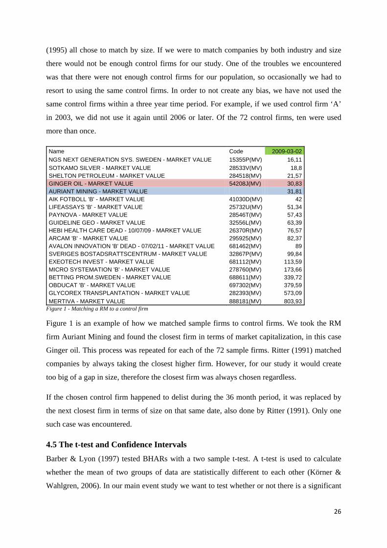
in 2003, we did not use it again until 2006 or later. Of the 72 control firms, ten were used

more than once.

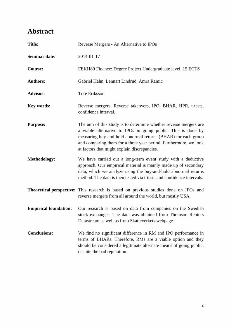
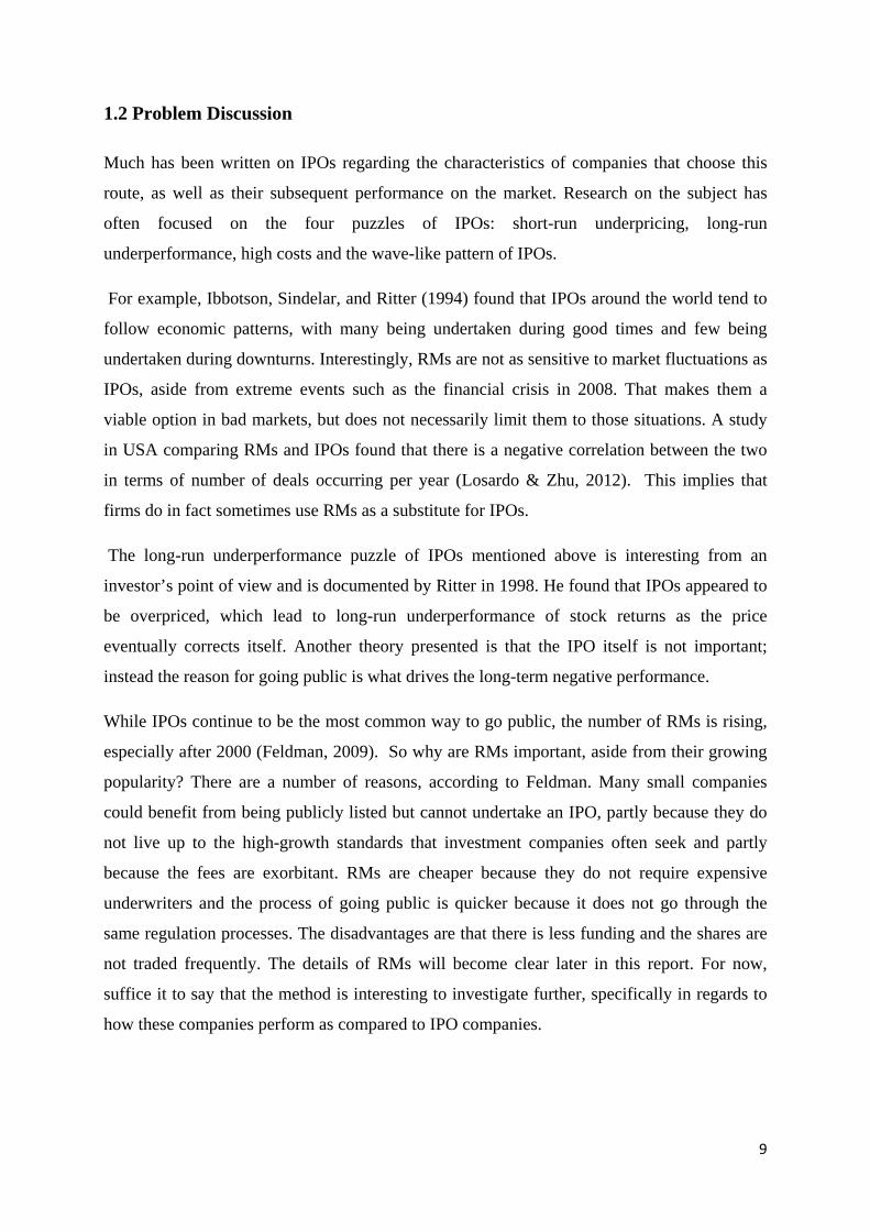
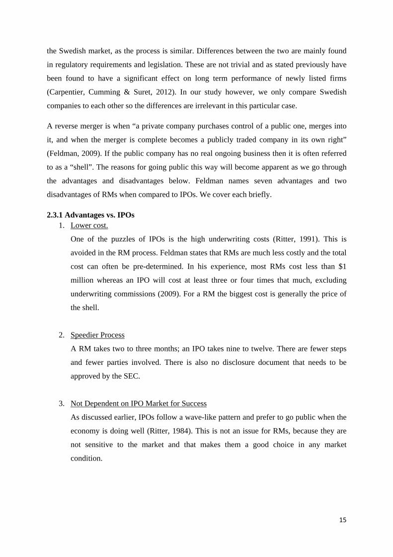
Name Code 2009-03-02 NGS NEXT GENERATION SYS. SWEDEN - MARKET VALUE 15355P(MV) 16,11 SOTKAMO SILVER - MARKET VALUE 28533V(MV) 18,8 SHELTON PETROLEUM - MARKET VALUE 284518(MV) 21,57 GINGER OIL - MARKET VALUE 54208J(MV) 30,83 AURIANT MINING - MARKET VALUE 31,81 AIK FOTBOLL 'B' - MARKET VALUE 41030D(MV) 42 LIFEASSAYS 'B' - MARKET VALUE 25732U(MV) 51,34 PAYNOVA - MARKET VALUE 28546T(MV) 57,43 GUIDELINE GEO - MARKET VALUE 32556L(MV) 63,39 HEBI HEALTH CARE DEAD - 10/07/09 - MARKET VALUE 26370R(MV) 76,57 ARCAM 'B' - MARKET VALUE 295925(MV) 82,37 AVALON INNOVATION 'B' DEAD - 07/02/11 - MARKET VALUE 681462(MV) 89 SVERIGES BOSTADSRATTSCENTRUM - MARKET VALUE 32867P(MV) 99,84 EXEOTECH INVEST - MARKET VALUE 681112(MV) 113,59 MICRO SYSTEMATION 'B' - MARKET VALUE 278760(MV) 173,66 BETTING PROM.SWEDEN - MARKET VALUE 688611(MV) 339,72 OBDUCAT 'B' - MARKET VALUE 697302(MV) 379,59 GLYCOREX TRANSPLANTATION - MARKET VALUE 282393(MV) 573,09 MERTIVA - MARKET VALUE 888181(MV) 803,93

Figure 1 - Matching a RM to a control firm

Figure 1 is an example of how we matched sample firms to control firms. We took the RM

firm Auriant Mining and found the closest firm in terms of market capitalization, in this case

Ginger oil. This process was repeated for each of the 72 sample firms. Ritter (1991) matched

companies by always taking the closest higher firm. However, for our study it would create

too big of a gap in size, therefore the closest firm was always chosen regardless.

If the chosen control firm happened to delist during the 36 month period, it was replaced by

the next closest firm in terms of size on that same date, also done by Ritter (1991). Only one

such case was encountered.

4.5 The t-test and Confidence Intervals Barber & Lyon (1997) tested BHARs with a two sample t-test. A t-test is used to calculate

whether the mean of two groups of data are statistically different to each other (Körner &

Wahlgren, 2006). In our main event study we want to test whether or not there is a significant

27

difference in RM and IPO mean BHARs. We take the mean BHAR for all the RMs and the

mean BHAR for all the IPOs annually and apply t-tests for year one, two, and three as shown

in formula 4. We also test the mean BHAR difference for RMs and IPOs via confidence

intervals for all 36 months as shown in formula 5.

𝑡𝐵𝐻𝐴𝑅 = (𝐵𝐻𝐴𝑅𝑅𝑀 − 𝐵𝐻𝐴𝑅𝐼𝑃𝑂)/(𝜎𝐵𝐻𝐴𝑅/√𝑛) (4)

𝐶𝑜𝑛𝑓𝑖𝑑𝑒𝑛𝑐𝑒 𝑖𝑛𝑡𝑒𝑟𝑣𝑎𝑙𝑅𝑀,𝐼𝑃𝑂 = (𝐵𝐻𝐴𝑅��������𝑅𝑀 − 𝐵𝐻𝐴𝑅��������𝐼𝑃𝑂) ± 𝑧 ∗ �𝑠𝑅𝑀2

𝑛𝑅𝑀+ 𝑠𝐼𝑃𝑂

2

𝑛𝐼𝑃𝑂 (5)

𝜎𝐵𝐻𝐴𝑅 is the standard deviation of BHAR and 𝑛 is the number of observations. According to

Körner & Wahlgren (2006), when testing a hypothesis you should determine the significance

level prior to the analysis. We chose a 95% significance level, as is common for this type of

study, which means that there is a 5% probability that the null hypothesis is rejected even if it

is true. Z is set to 1.96 which is the value used at the 95% significance level. Most statistical

programs do a t-test rather than a z-test but the difference is negligible for samples greater

than 30 and will suffice here as well.

To get an idea of how IPOs and RMs did in comparison to their benchmarks we also plotted

confidence intervals for their respective BHARs. That formula is given below:

𝐶𝑜𝑛𝑓𝑖𝑑𝑒𝑛𝑐𝑒 𝑖𝑛𝑡𝑒𝑟𝑣𝑎𝑙 = 𝐵𝐻𝐴𝑅�������� ± 𝑧 ∗ 𝑠𝐵𝐻𝐴𝑅√𝑛

(6)

Note that we could have just compared confidence intervals for IPOs and RMs; if they

overlap that would indicate that there is no significant difference. Plotting each set in one

graph would have made it unclear and we also wanted to analyze each separately.

4.6 Hypothesis Testing

Hypothesis testing consists of formulating a null hypothesis 𝐻0 and an alternative hypothesis

𝐻1. They are tested against each other through statistical methods and the null hypothesis is

either accepted or rejected (Körner & Wahlgren, 2006). Our null hypothesis for the main

event study is that there is no difference between RM and IPO BHAR means. The alternative

hypothesis is that there is a difference between RMs and IPOs. Ours is a two-tailed test,

meaning the difference can either be negative or positive.

As stated by Körner & Wahlgren (2006), when the sample size of the study is large enough,

n > 30, it is not necessary for the sample to be normally distributed in order to calculate

28

confidence intervals according to the central limit theorem. However, we graph histograms to

get an idea of what the distributions look like. This will help in the analysis.

Additionally, 95% confidence intervals are calculated and plotted on a graph for two more

studies; one on RMs versus their benchmark and the other on IPOs versus their benchmark.

Applying a t-test to all 36 months would have taken longer than just plotting and observing

whether or not the confidence interval covers zero. When it does, the null hypothesis cannot

be rejected. Furthermore, a graph shows potential trends which are useful when analyzing the

results.

𝐻0 = 𝑡ℎ𝑒𝑟𝑒 𝑖𝑠 𝑛𝑜 𝑠𝑖𝑔𝑛𝑖𝑓𝑖𝑐𝑎𝑛𝑡 𝑑𝑖𝑓𝑓𝑒𝑟𝑒𝑛𝑐𝑒 𝑏𝑒𝑡𝑤𝑒𝑒𝑛 𝑅𝑀 𝑎𝑛𝑑 𝐼𝑃𝑂 𝑚𝑒𝑎𝑛 𝐵𝐻𝐴𝑅𝑠

𝐻1 = 𝑡ℎ𝑒𝑟𝑒 𝑖𝑠 𝑎 𝑠𝑖𝑔𝑛𝑖𝑓𝑖𝑐𝑎𝑛𝑡 𝑑𝑖𝑓𝑓𝑒𝑟𝑒𝑛𝑐𝑒 𝑏𝑒𝑡𝑤𝑒𝑒𝑛 𝑅𝑀 𝑎𝑛𝑑 𝐼𝑃𝑂 𝑚𝑒𝑎𝑛 𝐵𝐻𝐴𝑅

29

5 Analysis and Results

5.1 Observation trends The sample in this study is comprised of 72 firms on the Swedish stock market; 36 RM firms

and 36 IPO firms. The selection is made according to the criteria in the methodology section.

The full list of RMs and IPOs along with their market capitalizations, date of deals, markets,

and matching companies can be found in appendix I.

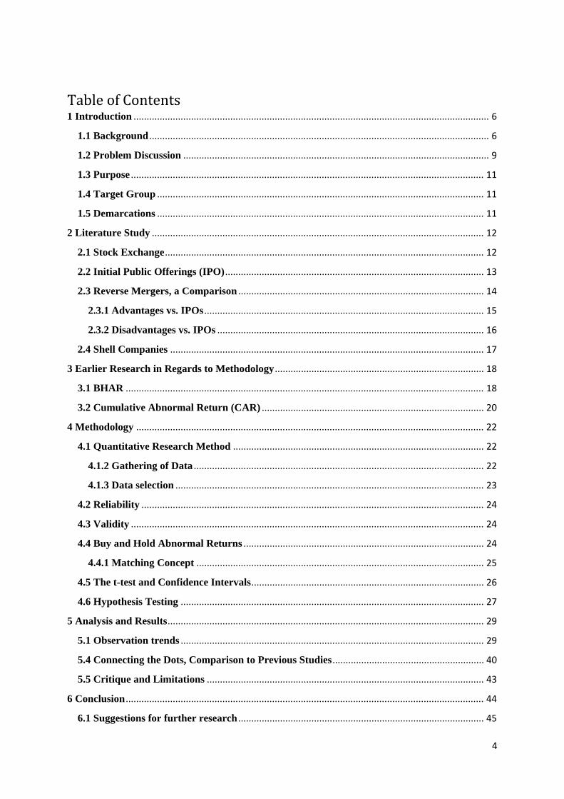
Table 1 and figure 1 show the distribution of consummated deals for IPOs and RMs

respectively during our time frame. The IPO data shows a clear drop in the number of deals

from 2000-2003 due to the IT crash but then picks up and peaks in 2007, only to fall again

when the financial crisis strikes in 2008. As expected, the IPO volume mimics the market

trend, peaking when market sentiment is high and dropping when it is low. The number of

RM deals is too small to draw any conclusions about trends, although there is a large increase

in 2005 and 2006.

Aggregate IPOs Aggregate RMs

Year # of IPOs Year # of RMs 2000 30 2000 1 2001 22 2001 1 2002 12 2002 3 2003 8 2003 2 2004 15 2004 1 2005 33 2005 8 2006 47 2006 7 2007 55 2007 4 2008 24 2008 2 2009 17 2009 5 2010 29 2010 2 TOTAL 292 Total 36

Table 1- RM and IPO distribution by year

A regression analysis done by Lhosardo & Zhu (2012) on RMs and IPOs in USA from 2004-

2011 yielded a significant negative correlation between the two groups. Our small sample of

This chapter will include a description of our data, as well as results and an analysis. It starts with trends of RMs and goes on to t-tests and confidence intervals. Lastly, a summary and comparison is made on previous research, followed by a critique and limitations.

30

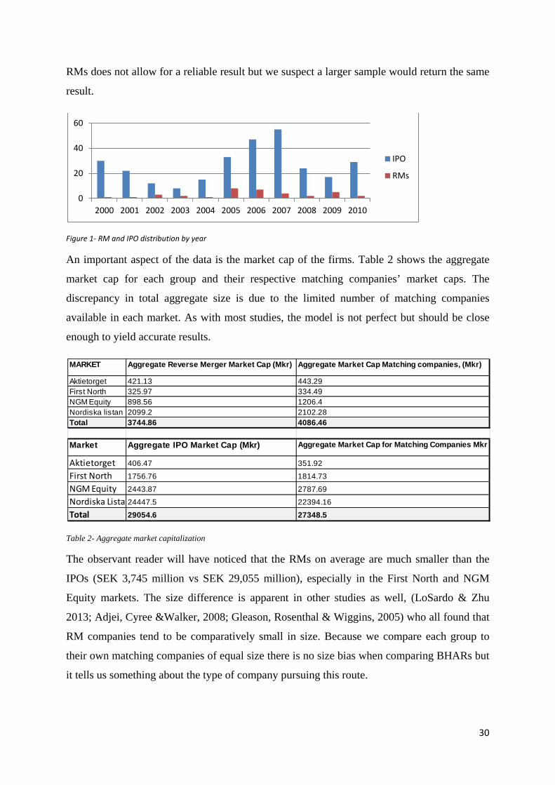
RMs does not allow for a reliable result but we suspect a larger sample would return the same

result.

Figure 1- RM and IPO distribution by year

An important aspect of the data is the market cap of the firms. Table 2 shows the aggregate

market cap for each group and their respective matching companies’ market caps. The

discrepancy in total aggregate size is due to the limited number of matching companies

available in each market. As with most studies, the model is not perfect but should be close

enough to yield accurate results.

Table 2- Aggregate market capitalization

The observant reader will have noticed that the RMs on average are much smaller than the

IPOs (SEK 3,745 million vs SEK 29,055 million), especially in the First North and NGM

Equity markets. The size difference is apparent in other studies as well, (LoSardo & Zhu

2013; Adjei, Cyree &Walker, 2008; Gleason, Rosenthal & Wiggins, 2005) who all found that

RM companies tend to be comparatively small in size. Because we compare each group to

their own matching companies of equal size there is no size bias when comparing BHARs but

it tells us something about the type of company pursuing this route.

0

20

40

60

2000 2001 2002 2003 2004 2005 2006 2007 2008 2009 2010

IPO

RMs

MARKET Aggregate Reverse Merger Market Cap (Mkr) Aggregate Market Cap Matching companies, (Mkr)

Aktietorget 421.13 443.29First North 325.97 334.49NGM Equity 898.56 1206.4Nordiska listan 2099.2 2102.28Total 3744.86 4086.46

Market Aggregate IPO Market Cap (Mkr) Aggregate Market Cap for Matching Companies Mkr

Aktietorget 406.47 351.92

First North 1756.76 1814.73

NGM Equity 2443.87 2787.69

Nordiska Lista 24447.5 22394.16

Total 29054.6 27348.5

31

We surmise that RMs are not yet a popular way to go public for large companies, which leads

us to believe that companies undertaking RMs most likely do not qualify for a regular IPO or

cannot afford one. The effect of those two aspects on performance are of interest to us, as

differences in regulations have been seen to negatively affect performance due to information

asymmetry (Carpentier, Cumming & Suret, 2012). For example, we found that NGM Equity

was the most popular place to undertake RMs and since regulations do differ between the

market places this may have an effect on performance. Testing each market against the others

would not be appropriate however, due to the small number of RMs in each.

5.2 T-test findings

5.2.1 Testing for normalcy

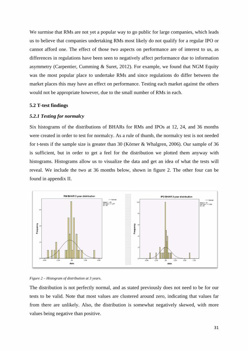
Six histograms of the distributions of BHARs for RMs and IPOs at 12, 24, and 36 months

were created in order to test for normalcy. As a rule of thumb, the normalcy test is not needed

for t-tests if the sample size is greater than 30 (Körner & Whalgren, 2006). Our sample of 36

is sufficient, but in order to get a feel for the distribution we plotted them anyway with

histograms. Histograms allow us to visualize the data and get an idea of what the tests will

reveal. We include the two at 36 months below, shown in figure 2. The other four can be

found in appendix II.

Figure 2 – Histogram of distribution at 3 years.

The distribution is not perfectly normal, and as stated previously does not need to be for our

tests to be valid. Note that most values are clustered around zero, indicating that values far

from there are unlikely. Also, the distribution is somewhat negatively skewed, with more

values being negative than positive.

32

Another criterion with t-tests is for the sample standard deviations to be equal. This was tested

with an F-test. The F-test is the two-tailed probability that the variances are not significantly

different. Table 3 shows the result of that test for 12, 24, and 36 months. None of the values

are lower than 0.05 so we conclude there is no significant difference in standard deviation.

However, note that, year two shows a large difference in variance and would have been

significant at a 90% level. We can now move on to the actual tests.

Table 3 - F-test for RMs and IPOs

5.2.2 Two-sample t-test

The delisted companies (three for RMs and seven for IPOs) mentioned earlier in the

methodology section pose somewhat of a problem when measuring BHAR. They exhibit

similar characteristics to each other in that they generally did poorly and shortly after delisting

went bankrupt. In order to deal with the potential survivorship bias this might cause, we carry

out two separate t-tests comparing BHAR means. One includes the delisted companies (using

the last known market value after the delisting) and one excludes them (truncated method)

after they delist. The purpose of this is to determine whether or not the bias changes the

results. The results are displayed in table 4. The tests are performed at year one, two and three

at the 95% significance level; the left column shows the results with delisted companies

included. The right column excludes them (revealing a potential survivorship bias). The null

hypothesis is that no difference exists between RMs and IPOs. Note the difference in

observations for each group and year.

1 Year RM BHAR 1 Year IPO BHAR 2 Year RM BHAR 2 Year IPO BHAR 3 Year RM BHAR 3 Year IPO BHARVariance 1.374919301 0.92518546 3.246790735 1.729095467 1.61541233 2.148349889Mean -0.24 -0.10 -0.19 -0.04 -0.29 0.01F-TEST 0.246145508 0.066410793 0.403175696

33

Table 4 - t-test including and excluding dead companies

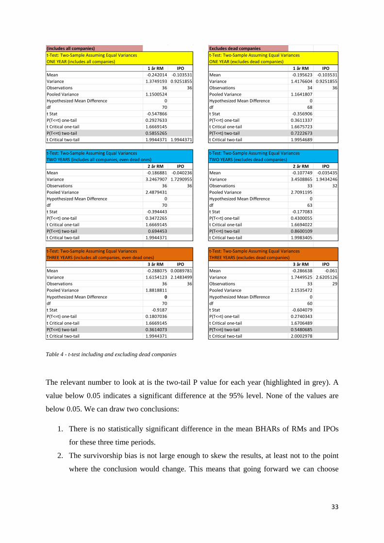
The relevant number to look at is the two-tail P value for each year (highlighted in grey). A

value below 0.05 indicates a significant difference at the 95% level. None of the values are

below 0.05. We can draw two conclusions:

1. There is no statistically significant difference in the mean BHARs of RMs and IPOs

for these three time periods.

2. The survivorship bias is not large enough to skew the results, at least not to the point

where the conclusion would change. This means that going forward we can choose

(includes all companies) Excludes dead companiest-Test: Two-Sample Assuming Equal Variances t-Test: Two-Sample Assuming Equal VariancesONE YEAR (includes all companies) ONE YEAR (excludes dead companies)

1 år RM IPO 1 år RM IPOMean -0.242014 -0.103531 Mean -0.195623 -0.103531Variance 1.3749193 0.9251855 Variance 1.4176604 0.9251855Observations 36 36 Observations 34 36Pooled Variance 1.1500524 Pooled Variance 1.1641807Hypothesized Mean Difference 0 Hypothesized Mean Difference 0df 70 df 68t Stat -0.547866 t Stat -0.356906P(T<=t) one-tail 0.2927633 P(T<=t) one-tail 0.3611337t Critical one-tail 1.6669145 t Critical one-tail 1.6675723P(T<=t) two-tail 0.5855265 P(T<=t) two-tail 0.7222673t Critical two-tail 1.9944371 1.9944371 t Critical two-tail 1.9954689

t-Test: Two-Sample Assuming Equal Variances t-Test: Two-Sample Assuming Equal VariancesTWO YEARS (includes all companies, even dead ones) TWO YEARS (excludes dead companies)

2 år RM IPO 2 år RM IPOMean -0.186881 -0.040236 Mean -0.107749 -0.035435Variance 3.2467907 1.7290955 Variance 3.4508865 1.9434246Observations 36 36 Observations 33 32Pooled Variance 2.4879431 Pooled Variance 2.7091195Hypothesized Mean Difference 0 Hypothesized Mean Difference 0df 70 df 63t Stat -0.394443 t Stat -0.177083P(T<=t) one-tail 0.3472265 P(T<=t) one-tail 0.4300055t Critical one-tail 1.6669145 t Critical one-tail 1.6694022P(T<=t) two-tail 0.694453 P(T<=t) two-tail 0.8600109t Critical two-tail 1.9944371 t Critical two-tail 1.9983405

t-Test: Two-Sample Assuming Equal Variances t-Test: Two-Sample Assuming Equal VariancesTHREE YEARS (includes all companies, even dead ones) THREE YEARS (excludes dead companies)

3 år RM IPO 3 år RM IPOMean -0.288075 0.0089781 Mean -0.286638 -0.061Variance 1.6154123 2.1483499 Variance 1.7449525 2.6205126Observations 36 36 Observations 33 29Pooled Variance 1.8818811 Pooled Variance 2.1535472Hypothesized Mean Difference 0 Hypothesized Mean Difference 0df 70 df 60t Stat -0.9187 t Stat -0.604079P(T<=t) one-tail 0.1807036 P(T<=t) one-tail 0.2740343t Critical one-tail 1.6669145 t Critical one-tail 1.6706489P(T<=t) two-tail 0.3614073 P(T<=t) two-tail 0.5480685t Critical two-tail 1.9944371 t Critical two-tail 2.0002978

34

just one of the two tests (we include them all) without jeopardizing the validity of the

results.

The most interesting test result here is for three years, showing no significant difference. This

implies that RMs did just as well as IPOs in the long run and should be a viable option for

firms and investors alike. Note however that for each year the mean BHAR was lower for

RMs than IPOs, raising our suspicions that perhaps there is more to the story. We return to

this later but first let us look at how the RMs and IPOs performed in comparison to their

benchmark (matching companies).

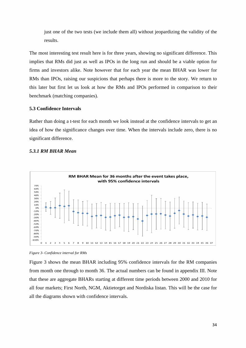
5.3 Confidence Intervals

Rather than doing a t-test for each month we look instead at the confidence intervals to get an

idea of how the significance changes over time. When the intervals include zero, there is no

significant difference.

5.3.1 RM BHAR Mean

Figure 3- Confidence interval for RMs

Figure 3 shows the mean BHAR including 95% confidence intervals for the RM companies

from month one through to month 36. The actual numbers can be found in appendix III. Note

that these are aggregate BHARs starting at different time periods between 2000 and 2010 for

all four markets; First North, NGM, Aktietorget and Nordiska listan. This will be the case for

all the diagrams shown with confidence intervals.

35

The 95% confidence intervals all pass through zero, indicating that there is no significant

difference between the RM companies and their matching companies, despite the distinct

negative performance after the seventh month. A 90% significance level test (not shown here)

gave similar results, showing a significant difference only in month 22. The intervals are quite

wide, more so than they perhaps should be despite the small sample size, given that the RM

companies consist of almost the whole population for that time period. A few may have been

missed due to the manual process of finding them but we believe the list to be otherwise

complete. If true, the mean BHAR values are quite accurate and the confidence intervals

should be narrower, perhaps even to the point where zero is not included.

All but the first six months show negative BHAR means. An investor buying an equal amount

of all the RMs at each starting point during this time period would have seen lower returns

than if the matching companies had been bought instead, albeit not significantly so.

This comparison is important because it is of interest to know not only how RMs performed

in relation to IPOs but also how each group performed in comparison to their respective

benchmarks. For example, Ritter (1991) attributes long term IPO underperformance to timing,

where companies mostly prefer going public during what he calls “industry specific fads”.

RMs on the other hand are not as dependent on market sentiment, they can be undertaken

even in bad markets and so the risk of overvaluation is decreased and we should perhaps see a

better relative performance. This did not hold true for the t-tests in figure 4 however. In fact

the IPOs had higher mean BHARs. A possible reason is that timing is only one of many

factors affecting the performance; stock trading volume for example has been found to

significantly impact performance and would act in favor of IPOs since underwriters often

guarantee liquidity for a certain time after the offering (Lhosardo and Zhu, 2012).

36

5.3.2 IPO BHAR Mean

Next we study IPOs and compare them to their benchmark.

Figure 4 - IPO BHAR mean confidence interval

Figure 4 shows the same BHAR diagram as Figure 3 but this time for IPOs during the same

time period. Actual numbers are displayed in Appendix IV.

The confidence interval includes zero for all months, which leads us to not reject the null

hypothesis that the means are equal. There is no clear trend and the values seem to lie closer

to zero than for RMs, although only five of the months show a mean BHAR above zero. We

can conclude that IPOs have not underperformed the market at the 95% confidence level for

this sample and time period. This goes against what Ritter (1991) found for IPOs but is in line

with other studies, like one we found in Switzerland where IPOs did not underperform

matching companies when comparing to a small cap index (Drobetz, Kammermann &

Wälchli, 2005). They attribute the difference to what benchmark is used.

A study done on the Swedish market from 1998-2007 found that IPO firms over a three year

time horizon underperformed their market index and that the underperformance increased

over time (Lakkonen & Åkesson, 2007).The benchmark used was the OMX market index

which does not take into account the market size of IPOs so this further supports the Swiss

conclusion.

37

A longer time period or larger sample could possibly yield different results here as most

studies on IPO BHARs are stretched for longer than three years. Taking the full population of

IPOs would have been optimal but was not possible due to time constraints.

5.3.3 RM vs IPO BHAR Mean

Figure 5 - Confidence interval difference between IPO and RM BHAR means

Figure 5 shows the confidence intervals for the difference in means of RM companies and

IPOs, where a negative number signifies a poorer performance for RMs. This is the main

event-study in this paper. Actual numbers are displayed in Appendix V. Each interval for the

36 months includes zero which means the null hypothesis cannot be rejected. However, only

five months show a positive BHAR and they are clustered around the first six months. Note

that the confidence intervals are again very wide, which makes the comparison less useful

than it would have been with a larger sample or lower standard deviation. That problem might

be remedied in future studies should RMs become a more accepted means of going public.

We thought it prudent to also compare the mean BHARs of IPOs and RMs in one graph.

Figure 6 illustrates their respective trends in relation to each other.

38

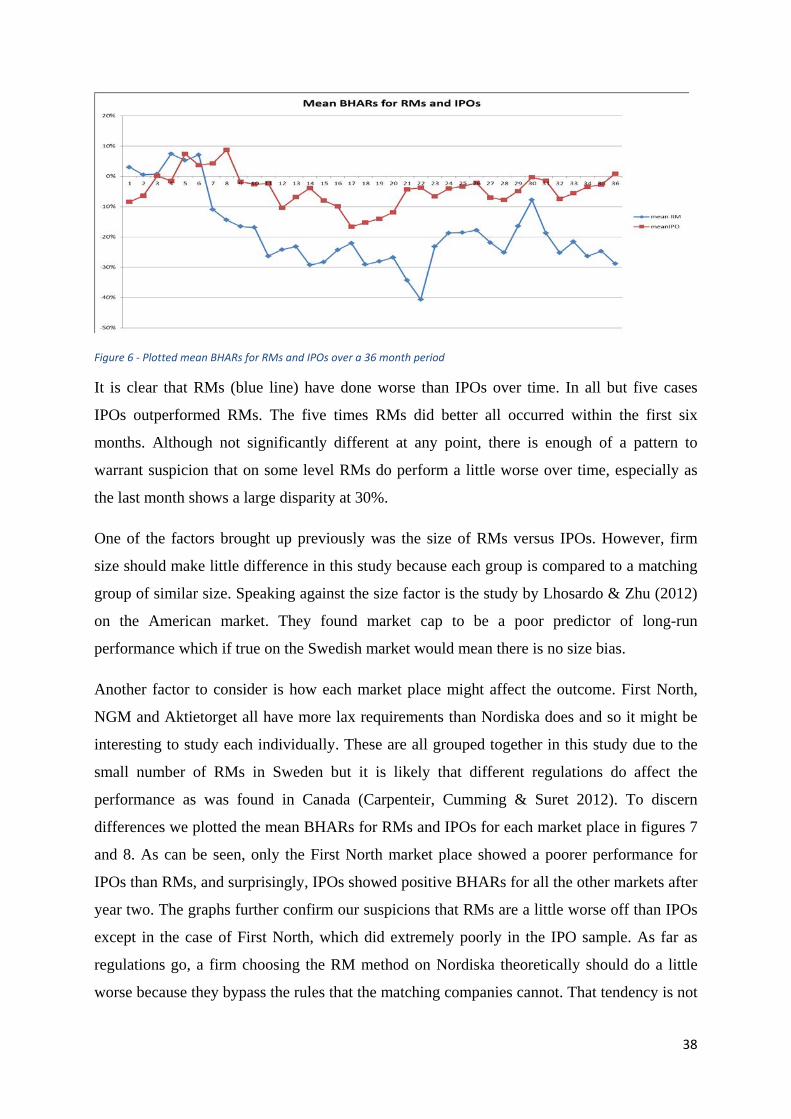
Figure 6 - Plotted mean BHARs for RMs and IPOs over a 36 month period

It is clear that RMs (blue line) have done worse than IPOs over time. In all but five cases

IPOs outperformed RMs. The five times RMs did better all occurred within the first six

months. Although not significantly different at any point, there is enough of a pattern to

warrant suspicion that on some level RMs do perform a little worse over time, especially as

the last month shows a large disparity at 30%.

One of the factors brought up previously was the size of RMs versus IPOs. However, firm

size should make little difference in this study because each group is compared to a matching

group of similar size. Speaking against the size factor is the study by Lhosardo & Zhu (2012)

on the American market. They found market cap to be a poor predictor of long-run

performance which if true on the Swedish market would mean there is no size bias.

Another factor to consider is how each market place might affect the outcome. First North,

NGM and Aktietorget all have more lax requirements than Nordiska does and so it might be

interesting to study each individually. These are all grouped together in this study due to the

small number of RMs in Sweden but it is likely that different regulations do affect the

performance as was found in Canada (Carpenteir, Cumming & Suret 2012). To discern

differences we plotted the mean BHARs for RMs and IPOs for each market place in figures 7

and 8. As can be seen, only the First North market place showed a poorer performance for

IPOs than RMs, and surprisingly, IPOs showed positive BHARs for all the other markets after

year two. The graphs further confirm our suspicions that RMs are a little worse off than IPOs

except in the case of First North, which did extremely poorly in the IPO sample. As far as

regulations go, a firm choosing the RM method on Nordiska theoretically should do a little

worse because they bypass the rules that the matching companies cannot. That tendency is not

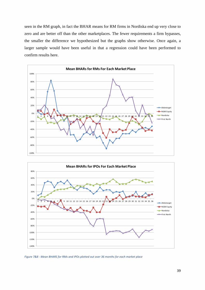
39

seen in the RM graph, in fact the BHAR means for RM firms in Nordiska end up very close to

zero and are better off than the other marketplaces. The fewer requirements a firm bypasses,

the smaller the difference we hypothesized but the graphs show otherwise. Once again, a

larger sample would have been useful in that a regression could have been performed to

confirm results here.

Figure 7&8 - Mean BHARS for RMs and IPOs plotted out over 36 months for each market place

-100%

-80%

-60%

-40%

-20%

0%

20%

40%

60%

80%

100%

1 2 3 4 5 6 7 8 9 10 11 12 13 14 15 16 17 18 19 20 21 22 23 24 25 26 27 28 29 30 31 32 33 34 35 36

Mean BHARs for RMs For Each Market Place

Aktietorget

NGM Equity

Nordiska

First North

-140%

-120%

-100%

-80%

-60%

-40%

-20%

0%

20%

40%

60%

80%

1 2 3 4 5 6 7 8 9 10 11 12 13 14 15 16 17 18 19 20 21 22 23 24 25 26 27 28 29 30 31 32 33 34 35 36

Mean BHARs for IPOs For Each Market Place

Aktietorget

NGM Equity

Nordiska

First North

40

5.4 Connecting the Dots, Comparison to Previous Studies Table 5 presents a brief summary on RM studies, most of which have been mentioned earlier.

There are others, but we felt these were the most interesting and this summary should make it

easier when analyzing differences in results. They span the whole world and as such provide

interesting information on possible reasons for discrepancies between nations with regards to

RM performance.

Authors Conclusion Gleason, K.C., Rosenthal, L. & Wiggins, R.A. (2005) “Backing into being public: an exploratory analysis of reverse takeovers.” (USA)

Small, young companies typically undertake RMs. Short term some gains can be seen but long term they usually fail to generate any wealth for shareholders. 46% have not survived two years. Still, they conclude it is an important mechanism, albeit a risky one for investors.

Carpentier, C., Cumming, D. & Suret, J-M. “The Value of Capital Market Regulation: IPOs Versus Reverse Mergers” (Canada)

High listing requirements decreases information asymmetry and significantly affects long term performance positively. Mostly low quality firms choose the RM route. They conclude IPOs are better due to more regulations but find that in Canada they performed similarly.

Adjei, F., Cyree, K.B. &Walker, M.M. “The Determinants and Survival of Reverse Mergers vs IPOs.” (USA)

Small, young companies with weak performance are typical for RMs. 42% of the companies delisted in the three year period study.

LoSardo, M.J. & Zhu, J. “A Further exploration of Reverse Takeovers as an alternative to IPOs” (USA)

Find that RMs did better than the American index. Find that good performance is correlated with trading activity. See RMs as positive.

Brown, P., Ferguson A. & Lam, P. “Choice between alternative routes to go public: backdoor listing vs IPO” (Australia)

Poor long term performance for RMs, even short term gains are small and underpricing is often present. The RM route is not always an easier and quicker way to go and appears to not always be chosen by small companies.

Roosenboom, P. & Schramade, W. “ Reverse Mergers in the United Kingdom: listed targets and private acquirers” (UK)

Long-run performance similar independent of listing route. Short-run target returns are positive and the bigger the private acquiring company relative to the public target is, the larger the abnormal returns are.

Table 5- A summary of previous research

41

Performance

Our study shows no significant difference in BHARs between RMs and IPOs. Of the studies

above, two have the same outcome, while three do not. Not all studies were focused on

performance however, like Adjei, Cyree & Walker (2008), who mainly looked at the reasons

for undertaking RMs in the first place and how many survived. The two studies where RM

performances matched or surpassed IPOs were done in the UK and USA respectively.

Perhaps RMs are turning into a more accepted means of going public, making investors less

likely to eschew them. In USA the SEC has sharpened rules and by so doing improved the

legitimacy of RMs. If more investors are willing to invest in these companies, the

performance should improve.

Size

The size of the companies taking the RM route was perhaps the most common denominator in

all the studies. All but one (Australia) found that the companies were small in comparison to

IPOs. However, as stated previously, a regression by Lhosardo & Zhu (2012) (USA) based on

market cap revealed no significant correlation to performance. Instead they found that stock

volume traded the first few days was a good indicator of future performance, the higher the

better. We find this interesting because theoretically IPOs should have higher turnover of their

common stock post-event than RMs do, with underwriters acting as market makers.

Consequently, they should do better over time but that trend is not clear in our case.

Delistings

Fewer companies delisted on the Swedish exchanges than the American one as found by

Gleason, Rosenthal &Wiggins (2005) and Adjei, Cyree & Walker (2008) who both saw over

40% of RMs delisted for three and two years respectively. In Sweden that number is 17% in

the first three years. While delisting generally involves poor performance for these firms, we

think it says little about the total performance of RMs as a group. In the mentioned studies, no

study was conducted for the long-term BHAR.

Regulation effects

Our results reveal that RMs did not do worse on Nordiska, as should have been the case if

regulations play a role in performance. We surmise that they play less of a role in Sweden but

with the caveat that our sample is too small in each market place for a good judgment to be

42

made. In Canada there was a significant difference for how the firms performed as compared

to other countries but not so much between the RMs and IPOs in Canada alone. This tells us

something about RMs, they are viable but like most other companies might benefit from

stricter regulations.

Shell and merger characteristics

In UK, the relative size of the acquiring company to the acquiree was found to make a

difference in how well the firms performed. Larger acquirers did better post-merger. Although

we did not cover this in our study, it is interesting to note because it could explain some of the

differences in the RM performance. Also, as is the case for a majority of mergers, the

acquired company (shell) receives most of the benefits of the merge. An interesting study was

done in 2011 by Floros & Sapp in USA which focused on shells rather RMs. They found that

the shell owners would have seen three-month abnormal returns of 48.1%. This was partly

negated by the high risk of owning illiquid stocks. Floros & Sapp (2011) also analyze the

characteristics of RM companies and find them to be small, young, and unprofitable.

Sectors

Another possible performance-driving factor not yet discussed is industry sectors. Only one

study brings this up, although indirectly. As mentioned earlier, Brown, Ferguson & Lam

(2010), found that RMs performed worse than their counterparts in Australia. They also

noticed that RM deals were more prevalent among high-tech companies. We conjecture that

one possible reason for the different outcomes between countries could be the sector fads at

certain times. For example, the IT sector would have seen extreme growth during the 90s, as

opposed to the industrial sector during the same time.

43

5.5 Critique and Limitations All studies have their shortcomings, which can be discussed and criticized. In order to allow a

fair assessment of our results, we include them here.

Time frame

Different markets/industries

Population

Beta

We use a time frame of ten years. During this time two major market crashes occurred. These

extreme events are not likely to be repeated every decade, and the effects are unpredictable. A

study from 2000 to 2010 is not necessarily comparable to other ten year event studies, e.g. a

study performed from 1980 to 1990. Therefore it is hard to generalize in regards to the result.

Additionally, a longer time-frame would yield a more conclusive result.

Our data consists of companies that operate on different exchanges and as such there are

different regulations when firms go public as well as different regulations when they are

listed. NASDAQ OMX and NGM have stricter requirements whereas Aktietorget and First

North are more lax. The effects of these requirements have not been tested statistically; we

graphed the BHAR means for each group to discern patterns but cannot say anything

conclusive.

We did not consider beta when matching companies to our samples of RMs and IPOs. In

theory, high betas indicate higher performance and higher volatility when compared to a

market index. Buying higher beta firms should therefore lead to better returns because the risk

is higher. However, we do not think this would have led to different results in our study, as

beta can be measured for different time periods and also changes over time, but it is worth

mentioning.

Population – We gathered practically the whole universe of undertaken RMs in the given time

frame but the sample is still quite small. The variance of the groups is high so the confidence

intervals had a large span as can be seen in the results. Consequently, the results are not as

strong as we would have liked and they should be assessed with that in mind. This is the one

weakness we believe might have enough of an effect to possibly change the outcome.

44

6 Conclusion

We find no significant difference in RM and IPO performance in terms of BHARs. Therefore,

RMs are a viable option and they should be considered a legitimate alternate means of going

public, despite the bad reputation. This conclusion is based on a premise that long-term

performance is a good indicator of what should and should not be allowed on the market. We

think it is, since we believe that the market eventually values a company correctly over time.

Ben Graham, known as Warrens Buffets mentor, once expressed it in the following way:

"In the short-run, the market is a voting machine - reflecting a voter-registration test that

requires only money, not intelligence or emotional stability - but in the long-run, the market is

a weighing machine" (Buffett & Cunningham, 2001).

While we do hold some reservation about the results due to sample size and the clear negative

results after the fifth month, previous studies in USA and UK have also come to the same

conclusions we have. As the reader may recall, the purpose of this study was two-fold. One

was to measure and compare the actual BHARs, and the other was to identify factors

influencing the performance for RMs if a difference was found. We did not apply any

regressions because there was no significant difference in the BHAR means. However, we

found that previous studies indicate a number of possible factors that affect long-run abnormal

returns positively: institutional ownership, liquidity of the stock, industry fads, difference in

size of the merging companies, and regulatory requirements on different stock exchanges.

Our findings on RMs should have some implications for the markets in Sweden. They have

turned out to be sustainable investments, though volatile. As such, companies should not be

afraid to use the method when it benefits them. The two most compelling reasons to us a RM

as opposed to IPOs is the low price-tag and the shorter time it takes. Going back to the

introduction, Candyking may have gone through with the IPO if investors had not reacted

negatively. A longer timeframe increases the probability of negative events occurring. For

In this chapter we present our conclusions of the study. We end with suggestions for further research.

45

RMs, the process is shorter and even if they do occur, decisions are made by the company

itself and valuations are more likely to be rational.

As for individual investors, RM companies are no better or worse off than any other but in our

opinion each should be valued on its own individual merits before any investment is made.

The high volatility of these stocks likely makes them unsuitable for all but the most intrepid

investors.

6.1 Suggestions for further research While writing this paper, we were made aware of a number of aspects in the subject that

would be interesting to pursue further. One is the shell-company aspect of the RMs. It would

be interesting to find out if the owners of the shell companies benefited from the RM and if a

strategy of buying them as an investor would have been profitable. A regression with a

number of independent variables like market-cap, price-to-book, trading activity, and

institutional ownership for RMs and IPOs would also have been interesting in order to find

out what drives long-term performance for each group. Also, a study using a larger time-span

could be used for further research on RMs in Sweden.

46

7 Bibliography 7.1 Articles Adjei, F., Cyree, K.B. & Walker, M.M. (2008) The determinants and survival of reverse mergers vs. IPOs. Journal of Economics and Finance, 32 (2), pp. 176-194. Barber, B.M., Lyon, J.D., (1997), Detecting long-run abnormal stock returns: the empirical power and specification of test statistics, Journal of Financial Economics, 43, pp. 341–373. Brown, P., Ferguson, A., Lam, P. (2010). Choice between alternative routes to go public: Backdoor listing versus IPO. Unpublished working paper. University of New South Wales and University of Technology Sydney. Carpentier, C., Cumming, D.J. & Suret, J-M. (2012) The Value of Capital Market Regulation: IPOs Versus Reverse Mergers, Journal of Empirical Legal Studies, 9 (1), pp. 56-91 Chen, H. Ritter, J. (2000) The Seven Percent Solution, Journal of Finance, 55, pp. 1105-1132. Drobetz, W., Kammermann, M. & Wälchli, U. (2005) Long-Run Performance of Initial Public Offerings: The Evidence for Switzerland, Schmalenbach Business Review, 57(3), pp. 253-275. Fama, E.F., & French, K.R. (1993) Common risk factors in the returns on stocks and bonds. Journal of financial economics, 33(1), pp. 3-56. Floros, I., Sapp, T., (2011) Shell games: On the value of shell companies. Journal of Corporate Finance 17, pp. 850-867. Gleason K.C., Rosenthal, L. & Wiggins, R.A. (2005) Backing into being public: an explanatory analysis of reverse takeovers, Journal of Corporate Finance, 12, pp. 54-79. Gleason, K. C., Jain, R., & Rosenthal, L. (2006) Alternatives for going public: evidence from reverse takeovers, self-underwritten IPOs, and traditional IPOs. Working Paper. Ibbotson, R.G., Ritter J.R. & Sindelar, J.L. (1994) The Market's Problems with the Pricing of Initial Public Offerings, Journal of Applied Corporate Finance, 7 (1), pp. 66-74. Lakkonen, T. & Åkesson, Elisabet. (2007) Dual Class Share Structure and IPO Long-Run Performance. Unpublished Master thesis. Stockholm School of Economics. Lee, O., Lochhead, S., Ritter, J. & Zhao, Q. (1996) The costs of raising capital. The Journal of Financial Research, 19 (1), pp. 59-74.

47

LoSardo, M. & Zhu, J. (2012) A Further Exploration of Reverse Takeovers as an Alternative to Initial Public Offerings. Unpublished bachelor thesis. Duke University. Loughran, T. & Ritter, J.R. (1995) The new issues puzzle. Journal of Finance 50 (1), p. 23-51. Ritter, J. R. (1984) The “hot issue” market of 1980, Journal of Business, 57 (2), pp. 215-240 Ritter, J. R. (1991) The Long-Run Performance of Initial Public Offerings, Journal of Finance, 46 (1), pp. 3-27 Ritter, J. R. (1998) Initial Public Offerings, Contemporary Finance Digest, 2 (1), pp. 5-30 Ritter, J.R (2011) Initial Public Offerings: Tables updated through 2011 Ritter, J.R. & Welch, I. (2002) A review of IPO activity, pricing, and allocations. The Journal of finance, 57 (4), pp. 1795-1828. Roosenboom, P.G.J. & Schramade, W.L.J. (2007). Reverse mergers in the UK: Listed targets and private acquirers. In G.N. Gregoriou & L. Renneboog (Eds.), International Mergers & Acquisitions Activity since 1990: Recent Research and Quantitative Analysis (pp. 181-194). Burlington: Academic Press / Elsevier. Rock, K. (1986) Why new issues are underpriced. Journal of Financial Economics, 15 (2), pp.197-212. 7.2 Literary sources Bell, E. & Bryman, A. (2007) Business research methods. Oxford: Oxford University Press. Berk, J.B. & DeMarzo, Peter M. (2013). Corporate finance. 3. ed., global ed. Harlow, England: Pearson. Bok Buffett, W., & Cunningham, L. A. (2001). The essays of Warren Buffett: lessons for corporate America. Cardozo Law Review. Feldman, D.N. (2009) Reverse Mergers: And Other Alternatives to Traditional IPOs. 2. ed., Hoboken: John & Wiley & Sons, Inc. Körner, S., & Wahlgren, L. (2006) Statistisk dataanalys. 4. ed., Lund: Studentlitteratur.

48

7.3 Digital sources Aktietorget (2013) Lista Ditt Bolag. Available at: http://www.aktietorget.se/CompanyListing.aspx?Language=1, 2014-01-05 Bernholm, J. (2011). Omvänt förvärv banar väg för bedragarna. Aktiespararna, 3. Available at: http://www.aktiespararna.se/Artikelarkiv/Repotage/2011/mars/Omvant-forvarv-banar-vagen-for-bedragarna/?lb=no&kampanj=pop-up-nej-tack. 2013-11-20

Finansinspektionen. Börsbolag. Available at: http://www.fi.se/Regler/Borsbolag/. 2013-11-28 First North listings Available at: http://www.nasdaqomx.com/listing/europe/growthmarket/, 2013-11-24 Regeringens Proposition 2001/02:165. Skatteregler mot handel med skalbolag. Stockholm: Finansdepartementet. Konjunkturterminologi. (2011) Available at: http://www.konj.se/download/18.70c52033121865b1398800099353/Konjunkturterminologi.pdf 2013-12-20. NASDAQ OMX (2014) Rule Book for Issuers NASDAQ OMX Stockholm. Available at: http://www.nasdaqomx.com/digitalAssets/89/89143_nasdaq-omx-stockholm-rule-book-for-issuers---1-januari-2014.pdf, 2014-01-08 NASDAQ OMX (2013) First North Nordic - Rulebook Available at: http://www.nasdaqomx.com/digitalAssets/86/86502_firstnorthrulebook2013-07-01_new2.pdf, 2013-11-24 Nordic Growth Market Available at: http://www.ngm.se/, 2013-11-24 Placera. (2008) Candyking vinstvarnar på börsupploppet. 11 December 2013. Available at: https://www.avanza.se/placera/redaktionellt/2013/12/11/candyking-vinstvarnar-pa-borsupploppet.html, 2014-01-06

Securities Exchange Act of 1934: Rule 12b-2, U.S Securities and Exchange Commission Available at: http://www.law.uc.edu/sites/default/files/CCL/34ActRls/rule12b-2.html, 2013-11-26 Skatteverket (2013) Aktiehistorik Available at: http://www.skatteverket.se/privat/skatter/vardepapperforsakringar/aktiermm/aktiehistorik.4.dfe345a107ebcc9baf80009051.html, 2013-11-15 Stockholmsbörsen/Nordiska Available at: http://www.nasdaqomxnordic.com, 2013-11-19

49

7.4 Databases Thomson Reuters DataStream. Available through LINC-lab, Ekonomihögskolan, Lund University

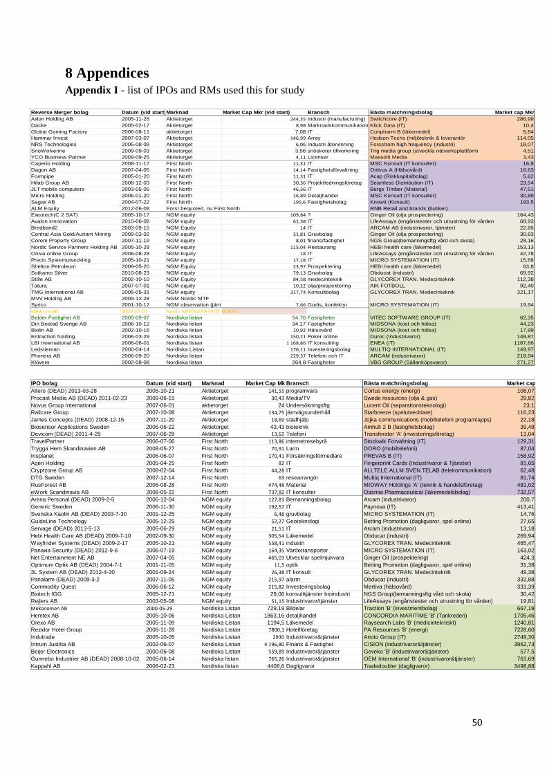
50

IPO bolag Datum (vid start) Marknad Market Cap Mkr Bransch Bästa matchningsbolag Market cap Altero (DEAD) 2013-03-28 2005-10-21 Aktietorget 141,55 programvara Cortus energy (energi) 108,07Procast Media AB (DEAD) 2011-02-23 2009-06-15 Aktietorget 30,43 Media/TV Swede resources (olja & gas) 29,82Novus Group International 2007-06-01 aktietorget 24 Undersökningsftg Lucent Oil (separationsteknologi) 23,1Railcare Group 2007-10-08 Aktietorget 134,75 järnvägsunderhåll Starbreeze (spelutvecklare) 116,23James Concepts (DEAD) 2008-12-15 2007-11-20 Aktietorget 18,69 städhjälp Jojka communications (mobiltelefoni program/apps) 22,18Biosensor Applications Sweden 2006-06-22 Aktietorget 43,43 bioteknik Amhult 2 B (fastighetsbolag) 39,48Devicom (DEAD) 2011-4-29 2007-06-29 Aktietorget 13,62 Telefoni Transferator 'A' (investeringsföretag) 13,04TravelPartner 2006-07-06 First North 113,86 internetresebyrå Stockwik Forvaltning (IT) 129,31Trygga Hem Skandinavien AB 2008-05-27 First North 70,91 Larm DORO (mobiltelefoni) 87,04Insplanet 2006-06-07 First North 170,41 Försäkringsförmedlare PREVAS B (IT) 158,92Aqeri Holding 2005-04-25 First North 82 IT Fingerprint Cards (Industrivaror & Tjänster) 81,65Cryptzone Group AB 2008-02-04 First North 44,28 IT ALLTELE ALLM.SVEN.TELAB (telekommunikation) 62,48DTG Sweden 2007-12-14 First North 63 researrangör Multiq International (IT) 81,74RusForest AB 2006-08-28 First North 474,48 Material MIDWAY Holdings 'A' (teknik & handelsföretag) 481,02eWork Scandinavia AB 2008-05-22 First North 737,82 IT konsulter Oasmia Pharmaceutical (läkemedelsbolag) 732,57Arena Personal (DEAD) 2009-2-5 2006-12-04 NGM equity 127,83 Bemanningsbolag Arcam (industrivaror) 200,7Generic Sweden 2006-11-30 NGM equity 192,57 IT Paynova (IT) 413,41Svenska Kaolin AB (DEAD) 2003-7-30 2001-12-25 NGM equity 6,48 gruvbolag MICRO SYSTEMATION (IT) 14,76GuideLine Technology 2005-12-25 NGM equity 52,27 Geoteknologi Betting Promotion (dagligvaror, spel online) 27,65Servage (DEAD) 2013-5-13 2005-06-29 NGM equity 21,51 IT Arcam (industrivaror) 13,18Hebi Health Care AB (DEAD) 2009-7-10 2002-09-30 NGM equity 305,54 Läkemedel Obducat (industri) 269,94Wayfinder Systems (DEAD) 2009-2-17 2005-10-21 NGM equity 558,41 industri GLYCOREX TRAN. Medecinteknik 465,47Panaxia Security (DEAD) 2012-9-6 2006-07-19 NGM equity 164,35 Värdetransporter MICRO SYSTEMATION (IT) 163,02Net Entertainment NE AB 2007-04-05 NGM equity 465,03 Utvecklar spelmjukvara Ginger Oil (prospektering) 424,3Optimum Optik AB (DEAD) 2004-7-1 2001-11-05 NGM equity 11,5 optik Betting Promotion (dagligvaror, spel online) 31,383L System AB (DEAD) 2012-4-30 2001-09-24 NGM equity 26,38 IT konsult GLYCOREX TRAN. Medecinteknik 49,38Panalarm (DEAD) 2009-3-2 2007-11-05 NGM equity 215,97 alarm Obducat (industri) 332,88Commodity Quest 2006-06-12 NGM equity 215,82 Investeringsbolag Mertiva (hälsovård) 331,39Biotech IGG 2005-12-21 NGM equity 29,06 konsulttjänster bioindustri NGS Group(bemanningsftg vård och skola) 30,42Rejlers AB 2003-05-08 NGM equity 51,15 Industrivaror/tjänster LifeAssays (engånstester och utrustning för vården) 19,81Mekonomen AB 2000-05-29 Nordiska Listan 729,19 Bildelar Traction 'B' (investmentbolag) 667,19Hemtex AB 2005-10-06 Nordiska Listan 1863,16 detaljhandel CONCORDIA MARITIME 'B' (Tankrederi) 1705,46Orexo AB 2005-11-09 Nordiska Listan 1194,5 Läkemedel Raysearch Labs 'B' (medicintekniskt) 1240,81Rezidor Hotel Group 2006-11-28 Nordiska Listan 7800,1 Hotellföretag PA Resources 'B' (energi) 7228,60Indutrade 2005-10-05 Nordiska Listan 2930 Industrivaror&tjänster Anoto Group (IT) 2749,30Intrum Justitia AB 2002-06-07 Nordiska Listan 4 196,80 Finans & Fastighet CISION (industrivaror&tjänster) 3962,73Beijer Electronics 2000-06-08 Nordiska Listan 559,89 Industrivaror&tjänster Geveko 'B' (industrivaror&tjänster) 577,5Gunnebo Industrier AB (DEAD) 2008-10-02 2005-06-14 Nordiska listan 765,26 Industrivaror&tjänster OEM International 'B' (industrivaror&tjänster) 763,69Kappahl AB 2006-02-23 Nordiska listan 4408,6 Dagligvaror Tradedoubler (dagligvaror) 3498,88

8 Appendices Appendix I - list of IPOs and RMs used this for study

Reverse Merger bolag Datum (vid start)Marknad Market Cap Mkr (vid start) Bransch Bästa matchningsbolag Market cap MkrAxlon Holding AB 2005-11-28 Aktietorget 244,35 Industri (manufacturing) Switchcore (IT) 286,99Dacke 2005-02-17 Aktietorget 8,98 Marknadskommunikation Klick Data (IT) 10,4Global Gaming Factory 2006-08-11 aktietorget 7,08 IT Conpharm B (läkemedel) 5,84Hammar Invest 2007-03-07 Aktietorget 146,99 Array Hedson Techs (miljöteknik & leverantör 114,05NRS Technologies 2005-08-09 Aktietorget 6,06 Industri återvinning Forsstrom high frequency (industri) 18,07SnoWolverine 2009-09-03 Aktietorget 3,56 snöskoter tillverkning Trig media group (utveckla nätverksplattform 4,51YCO Business Partner 2009-09-25 Aktietorget 4,11 Licenser Massolit Media 3,43Caperio Holding 2008-11-17 First North 11,31 IT MSC Konsult (IT konsulter) 16,8Dagon AB 2007-04-05 First North 14,14 Fastighetsförvaltning Ortivus A (Hälsovård) 16,63Formpipe 2005-01-20 First North 11,31 IT Acap (Riskkapitalbolag) 5,62Hifab Group AB 2008-12-03 First North 30,36 Projektledningsföretag Seamless Distribution (IT) 23,54JLT mobile computers 2003-05-05 First North 46,36 IT Bergs Timber (Material) 47,51Micro Holding 2006-01-20 First North 16,89 Detaljhandel MSC Konsult (IT konsulter) 30,89Sagax AB 2004-07-22 First North 195,6 Fastighetsbolag Knowit (Konsult) 193,5ALM Equity 2012-06-08 Först bequoted, nu First North RNB Retail and brands (butiker)Exeotech(C 2 SAT) 2005-10-17 NGM equity 109,84 ? Ginger Oil (olja prospectering) 164,43Avalon innnovation 2010-06-08 NGM equity 61,38 IT LifeAssays (engånstester och utrustning för vården 68,93Bredband2 2003-09-15 NGM Equity 14 IT ARCAM AB (industrivaror, tjänster) 22,85Central Asia Gold/Auriant Mining 2009-03-02 NGM equity 31,81 Gruvbolag Ginger Oil (olja prospectering) 30,83Corem Property Group 2007-11-19 NGM equity 8,01 finans/fastighet NGS Group(bemanningsftg vård och skola) 28,16Nordic Service Partners Holding AB 2005-10-28 NGM equity 115,04 Restaurang HEBI health care (läkemedel) 153,13Oniva online Group 2006-08-28 NGM Equity 18 IT LifeAssays (engånstester och utrustning för vården 42,78Precio Systemutveckling 2005-10-21 NGM equity 17,18 IT MICRO SYSTEMATION (IT) 15,68Shelton Petroleum 2009-05-20 NGM Equity 23,97 Prospektering HEBI health care (läkemedel) 63,8Sotkamo Silver 2010-08-23 NGM equity 79,13 Gruvbolag Obducat (industri) 69,92Stille AB 2002-10-10 NGM Equity 84,58 medecinteknik GLYCOREX TRAN. Medecinteknik 112,38Tatura 2007-07-01 NGM equity 10,22 olja/prospektering AIK FOTBOLL 92,40TMG International AB 2005-05-31 NGM equity 317,74 Konsultbolag GLYCOREX TRAN. Medecinteknik 321,17MVV Holding AB 2009-12-28 NGM Nordic MTFSyrico 2001-10-12 NGM observation (jämf 7,66 Godis, konfektyr MICRO SYSTEMATION (IT) 19,94Medcore AB 2009-07-01 Nordic MTF(NU PÅ FIRST NORTHBalder Fastighet AB 2005-09-07 Nordiska listan 54,76 Fastigheter VITEC SOFTWARE GROUP (IT) 62,35Din Bostad Sverige AB 2006-10-12 Nordiska listan 34,17 Fastigheter MIDSONA (kost och hälsa) 44,23Biolin AB 2002-10-16 Nordiska listan 20,92 Hälsovård MIDSONA (kost och hälsa) 17,99Entraction holding 2006-03-29 Nordiska listan 150,21 Poker online Duroc (Industrivaror) 149,87LBI International AB 2006-08-01 Nordiska listan 1 168,86 IT konsulting ENEA (IT) 1187,66Ledstiernan 2000-04-14 Nordiska Listan 176,11 Investeringsbolag MULTIQ INTERNATIONAL (IT) 149,97Phonera AB 2006-09-20 Nordiska listan 229,37 Telefoni och IT ARCAM (industrivaror) 218,94Klövern 2002-08-08 Nordiska listan 264,8 Fastigheter VBG GROUP (Sällanköpsvaror) 271,27

51

Appendix II – Histograms for year 1 and 2

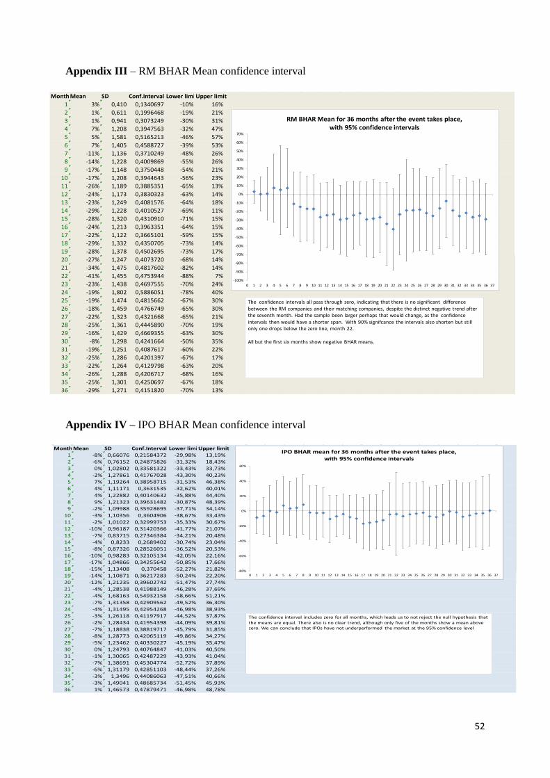
52

Appendix III – RM BHAR Mean confidence interval

Appendix IV – IPO BHAR Mean confidence interval

Month Mean SD Conf.Interval Lower limi Upper limit1 3% 0,410 0,1340697 -10% 16%2 1% 0,611 0,1996468 -19% 21%3 1% 0,941 0,3073249 -30% 31%4 7% 1,208 0,3947563 -32% 47%5 5% 1,581 0,5165213 -46% 57%6 7% 1,405 0,4588727 -39% 53%7 -11% 1,136 0,3710249 -48% 26%8 -14% 1,228 0,4009869 -55% 26%9 -17% 1,148 0,3750448 -54% 21%

10 -17% 1,208 0,3944643 -56% 23%11 -26% 1,189 0,3885351 -65% 13%12 -24% 1,173 0,3830323 -63% 14%13 -23% 1,249 0,4081576 -64% 18%14 -29% 1,228 0,4010527 -69% 11%15 -28% 1,320 0,4310910 -71% 15%16 -24% 1,213 0,3963351 -64% 15%17 -22% 1,122 0,3665101 -59% 15%18 -29% 1,332 0,4350705 -73% 14%19 -28% 1,378 0,4502695 -73% 17%20 -27% 1,247 0,4073720 -68% 14%21 -34% 1,475 0,4817602 -82% 14%22 -41% 1,455 0,4753944 -88% 7%23 -23% 1,438 0,4697555 -70% 24%24 -19% 1,802 0,5886051 -78% 40%25 -19% 1,474 0,4815662 -67% 30%26 -18% 1,459 0,4766749 -65% 30%27 -22% 1,323 0,4321668 -65% 21%28 -25% 1,361 0,4445890 -70% 19%29 -16% 1,429 0,4669355 -63% 30%30 -8% 1,298 0,4241664 -50% 35%31 -19% 1,251 0,4087617 -60% 22%32 -25% 1,286 0,4201397 -67% 17%33 -22% 1,264 0,4129798 -63% 20%34 -26% 1,288 0,4206717 -68% 16%35 -25% 1,301 0,4250697 -67% 18%36 -29% 1,271 0,4151820 -70% 13%

-100%

-90%

-80%

-70%

-60%

-50%

-40%

-30%

-20%

-10%

0%

10%

20%

30%

40%

50%

60%

70%

0 1 2 3 4 5 6 7 8 9 10 11 12 13 14 15 16 17 18 19 20 21 22 23 24 25 26 27 28 29 30 31 32 33 34 35 36 37

RM BHAR Mean for 36 months after the event takes place,with 95% confidence intervals

The confidence intervals all pass through zero, indicating that there is no significant difference between the RM companies and their matching companies, despite the distinct negative trend after the seventh month. Had the sample been larger perhaps that would change, as the confidence intervals then would have a shorter span. With 90% signifcance the intervals also shorten but still only one drops below the zero line, month 22.

All but the first six months show negative BHAR means.

Month Mean SD Conf.Interval Lower limi Upper limit1 -8% 0,66076 0,21584372 -29,98% 13,19%2 -6% 0,76152 0,24875826 -31,32% 18,43%3 0% 1,02802 0,33581322 -33,43% 33,73%4 -2% 1,27861 0,41767028 -43,30% 40,23%5 7% 1,19264 0,38958715 -31,53% 46,38%6 4% 1,11171 0,3631535 -32,62% 40,01%7 4% 1,22882 0,40140632 -35,88% 44,40%8 9% 1,21323 0,39631482 -30,87% 48,39%9 -2% 1,09988 0,35928695 -37,71% 34,14%

10 -3% 1,10356 0,3604906 -38,67% 33,43%11 -2% 1,01022 0,32999753 -35,33% 30,67%12 -10% 0,96187 0,31420366 -41,77% 21,07%13 -7% 0,83715 0,27346384 -34,21% 20,48%14 -4% 0,8233 0,2689402 -30,74% 23,04%15 -8% 0,87326 0,28526051 -36,52% 20,53%16 -10% 0,98283 0,32105134 -42,05% 22,16%17 -17% 1,04866 0,34255642 -50,85% 17,66%18 -15% 1,13408 0,370458 -52,27% 21,82%19 -14% 1,10871 0,36217283 -50,24% 22,20%20 -12% 1,21235 0,39602742 -51,47% 27,74%21 -4% 1,28538 0,41988149 -46,28% 37,69%22 -4% 1,68163 0,54932158 -58,66% 51,21%23 -7% 1,31358 0,42909562 -49,52% 36,30%24 -4% 1,31495 0,42954268 -46,98% 38,93%25 -3% 1,26118 0,41197917 -44,52% 37,87%26 -2% 1,28434 0,41954398 -44,09% 39,81%27 -7% 1,18838 0,38819717 -45,79% 31,85%28 -8% 1,28773 0,42065119 -49,86% 34,27%29 -5% 1,23462 0,40330227 -45,19% 35,47%30 0% 1,24793 0,40764847 -41,03% 40,50%31 -1% 1,30065 0,42487229 -43,93% 41,04%32 -7% 1,38691 0,45304774 -52,72% 37,89%33 -6% 1,31179 0,42851103 -48,44% 37,26%34 -3% 1,3496 0,44086063 -47,51% 40,66%35 -3% 1,49041 0,48685734 -51,45% 45,93%36 1% 1,46573 0,47879471 -46,98% 48,78%

-80%

-60%

-40%

-20%

0%

20%

40%

60%

0 1 2 3 4 5 6 7 8 9 10 11 12 13 14 15 16 17 18 19 20 21 22 23 24 25 26 27 28 29 30 31 32 33 34 35 36 37

IPO BHAR mean for 36 months after the event takes place, with 95% confidence intervals

The confidence interval includes zero for all months, which leads us to not reject the null hypothesis that the means are equal. There also is no clear trend, although only five of the months show a mean above zero. We can conclude that IPOs have not underperformed the market at the 95% confidence level

53

Appendix V – Confidence interval illustrating difference in means of RM and IPO BHAR means.

month X1-X2 conf intervlower limiupper limit1 11% 0,2541 -14% 37%2 7% 0,31897 -25% 39%3 1% 0,45522 -45% 46%4 9% 0,57471 -49% 66%5 -2% 0,64698 -67% 63%6 3% 0,5852 -55% 62%7 -15% 0,54662 -70% 39%8 -23% 0,5638 -80% 33%9 -15% 0,51938 -67% 37%

10 -14% 0,53438 -68% 39%11 -24% 0,50977 -75% 27%12 -14% 0,49543 -63% 36%13 -16% 0,49131 -65% 33%14 -25% 0,48289 -74% 23%15 -20% 0,51694 -72% 31%16 -14% 0,51006 -65% 37%17 -5% 0,50168 -56% 45%18 -14% 0,57143 -71% 43%19 -14% 0,57786 -72% 44%20 -15% 0,56816 -72% 42%21 -30% 0,63907 -94% 34%22 -37% 0,72648 -110% 36%23 -17% 0,63625 -80% 47%24 -15% 0,72869 -88% 58%25 -15% 0,63376 -79% 48%26 -16% 0,63502 -79% 48%27 -15% 0,58093 -73% 43%28 -17% 0,61206 -79% 44%29 -12% 0,61701 -73% 50%30 -8% 0,58831 -66% 51%31 -17% 0,58959 -76% 42%32 -18% 0,61789 -80% 44%33 -16% 0,59514 -75% 44%34 -23% 0,60937 -84% 38%35 -22% 0,64632 -87% 43%36 -30% 0,63375 -93% 34%

-120%

-100%

-80%

-60%

-40%

-20%

0%

20%

40%

60%

80%

0 1 2 3 4 5 6 7 8 9 10 11 12 13 14 15 16 17 18 19 20 21 22 23 24 25 26 27 28 29 30 31 32 33 34 35 36 37

CI for difference in means of RMs and IPOS at 95% significance level, for 36 months

The graph above shows the confidence intervals for the difference in means of RM companies and IPO companies. Each interval for the 36 months includes zero which means the null hypothesis cannot be rejected. However, only five of the 36 show a positive BHAR and they are clustered around the first six months. Note that the confidence intervals are very large, which makes the comparison less useful than it would have been with a larger sample or lower standard deviation.

54