Reverberation-Ray Matrix Analysis of Acoustic Waves in

2

Reverberation-Ray Matrix Analysis of Acoustic Waves in Multilayered Anisotropic Structures

Yongqiang Guo1 and Weiqiu Chen2 1Key Laboratory of Mechanics on Disaster and Environment in Western China, Ministry

of Education, and School of Civil Engineering and Mechanics, Lanzhou University 2Department of Engineering Mechanics, Zhejiang University

P.R.China

1. Introduction

Natural multilayers can be frequently observed, like the layered soils and rocks for example

(Kausel & Roesset, 1981; Kennett, 1983). They are also increasingly used as artificial

materials and structures in engineering practices for their high performances (Nayfeh, 1995).

For instances, cross-ply and fibrous laminated composites have been applied in naval

vessels, aeronautical and astronautical vehicles, and so on for the sake of high strength and

light weight (Nayfeh, 1995); piezoelectric thin film systems have been used in various

surface acoustic wave (SAW) and bulk acoustic wave (BAW) devices in electronics and

information technology in order to accomplish smaller size, lower energy consumption,

higher operating frequency and sensitivity, greater bandwidth, and enhanced reception

characteristics (Auld, 1990; Adler, 2000). Consequently, as a widespread category of

inhomogeneous materials and structures, multilayered structures deserve special concern

about their mechanical and acoustical behavior, especially the dynamic behavior since it is

what these structures differ most markedly from the homogeneous materials and structures.

Investigation of acoustic wave propagation in multilayered structures plays an essential role

in understanding their dynamic behavior, which is the main concern in design,

optimization, characterization and nondestructive evaluation of multilayered composites

(Lowe, 1995; Chimenti, 1997; Rose, 1999) and acoustic wave devices (Auld, 1990; Rose, 1999;

Adler, 2000). Nevertheless, the top and bottom surfaces and the interfaces in a multilayered

structure cause reflection and/or transmission of elastic waves, giving rise to coupling of

various fundamental wave modes in adjacent layers. In multilayered structures consisting of

anisotropic media, even the fundamental wave modes themselves are mutually coupled in

each layer (Achenbach, 1973). As a result, the analysis of acoustic waves in multilayered

structures always remains an extraordinary complex problem, and it is very difficult to

obtain a simple and yet numerically well-performed, closed-form analytical solution for a

general multilayered structure.

For the above reasons, various matrix formulations have been developed for the analysis of acoustic wave propagation in multilayered media from diverse domains (Ewing et al., 1957; Brekhovskikh, 1980; Kennett, 1983; Lowe, 1995; Nayfeh, 1995; Rose, 1999), since the beginning of this research subject in the midst of last century. Most of these matrix methods

Source: Acoustic Waves, Book edited by: Don W. Dissanayake, ISBN 978-953-307-111-4, pp. 466, September 2010, Sciyo, Croatia, downloaded from SCIYO.COM

www.intechopen.com

Acoustic Waves

26

were presented initially for multilayered structures consisting of isotropic (transversely isotropic) materials, and then extended to those structures made of anisotropic elastic and piezoelectric layers. These matrix methods fall into two groups. One group is those numerical methods based on discrete models, such as the boundary element method (BEM) (Makkonen, 2005), the finite difference method (FDM) (Igel et al., 1995; Makkonen, 2005), the finite element method (FEM) (Datta et al., 1988; Makkonen, 2005) and the hybrid method of BEM and FEM (BEM/FEM) (Makkonen, 2005). This group of methods is powerful for modeling acoustic waves in multilayered structures with various geometries and boundaries. However, they have the disadvantage that the results are approximate, and particularly certain high frequency components must be thrown off in any discrete model. The accuracy of the computational results and the stability of the numerical algorithms depend greatly on the discretization in the temporal and spatial domains. Calculation efficiency will be dramatically decreased if higher accuracy is pursued. The other group is those analytical methods based on continuous (distributed-parameter) model, among which the transfer matrix method (TMM) (Lowe, 1995), also referred to as the propagator matrix method (PMM) (Alshits & Maugin, 2008), is the typical one. TMM (Thomson, 1950; Haskell, 1953; Lowe, 1995; Nayfeh, 1995; Adler, 1990, 2000) leads to a system equation with dimension keeping small and unchanged as the number of layers increases, since in the formulation the basic unknowns of the intermediate layers are eliminated by matrix products. Thus, TMM has the advantage of high accuracy and high efficiency in most cases, but it suffers from numerical instability in the case of high frequency-thickness products (Nayfeh, 1995; Adler, 1990, 2000; Lowe, 1995; Tan, 2007). Aiming at circumventing this kind of numerical difficulty, different variant forms of TMM as well as analytical matrix methods have been proposed, including the stiffness matrix method (Kausel & Roesset, 1981; Shen et al., 1998; Wang & Rokhlin, 2001, 2002a; Rokhlin & Wang, 2002a; Tan, 2005), the spectral element method (Rizzi & Doyle, 1992; Chakraborty & Gopalakrishnan, 2006), the surface impedance matrix method (Honein et al., 1991; Degettekin et al., 1996; Zhang et al., 2001; Hosten & Castaings, 2003; Collet, 2004), the hybrid compliance/stiffness matrix method (Rokhlin & Wang, 2002b; Wang & Rokhlin, 2004a; Tan, 2006), the recursive asymptotic stiffness matrix method (Wang & Rokhlin, 2002b, 2004b, 2004c), the scattering matrix method (Pastureaud et al., 2002) and the compound matrix method (Fedosov et al., 1996), for instances. Tan (Tan, 2007) compared some of these methods in mathematical algorithm, computational efficiency and numerical stability. However, most of these alternative formulations lack uniformity in a certain degree, and are computationally complicated and inefficient, especially for the high frequency analysis. Lately, Pao and his coworkers (Pao et al, 2000; Su et al., 2002; Tian et al., 2006) developed the method of reverberation-ray matrix (MRRM) for evaluating the transient wave propagation in layered isotropic and transversely isotropic media. It is shown that MRRM has many advantages and its comparison to the TMM in various aspects was discussed by Pao et al. (Pao et al., 2007). However, the original formulation of MRRM is based on the wave potential functions, which confines this numerically stable and uniform matrix method from extending to layered anisotropic structures. In fact, it is impossible to use wave potential functions for an arbitrarily anisotropic medium, in which the fundamental wave modes are mutually coupled (Achenbach, 1973). Thus, Guo and Chen (Guo & Chen, 2008a, 2008b; Guo, 2008; Guo et al., 2009) presented a new formulation of MRRM based on state-space formalism and plane wave expansion for the analysis of free waves in anisotropic elastic and piezoelectric layered media.

www.intechopen.com


27

The objective of this chapter is to present the general and unified formulation of the method of reverberation-ray matrix (MRRM) for the analysis of acoustic wave propagation in multilayered structures of arbitrarily anisotropic elastic and piezoelectric media based on the state-space formalism and Fourier transforms. In Section 2, the state equation for each layer made of an arbitrarily anisotropic elastic/piezoelectric material is derived from the three-dimensional linear theory of elasticity/piezoelectricity with the help of Fourier transforms, and the solution to the state equation boils down to an eigenvalue problem from which the propagation constants and characteristic mode coefficients can be obtained numerically for a specified frequency. Then the traveling wave solution to the state equation can be written in explicit form in terms of unknown amplitudes as well as known propagation constants and characteristic mode coefficients. In Section 3, we show how the multilayered anisotropic structure is described in both the global and the local dual coordinates. From the boundary conditions on the upper and lower surfaces with applied external forces and the continuity conditions at the interfaces, the scattering relation, which expresses one group of equations for the unknown wave amplitudes in dual local coordinates, is appropriately constructed such that matrix inversion is avoided. Due to the uniqueness of physical essence, the two solutions expressed in dual local coordinates should be compatible with each other, leading to the phase relation, which represents the other group of equations for the unknown wave amplitudes in dual local coordinates. Care must be taken of to properly establish the phase relation such that all exponentially growing functions are excluded. The number of simultaneous equations from the phase and scattering relations amount exactly to the number of unknown wave amplitudes in dual local coordinates, and hence the wave solution can be determined. To reduce the dimension, we substitute the phase relation into the scattering relation to obtain a system equation, from which the dispersion relation for free wave propagation is obtained by letting the determinant of coefficient matrix vanish, and the steady-state and transient wave propagation due to the external force excitations can be obtained by inverse Fourier transforms. Section 4 gives numerical examples of guided wave propagation in cross-ply elastic composite structures. Dispersion curves for different configurations, various boundary conditions and in particular at the high frequency range are illustrated to show the versatility and numerical stability of the proposed formulation of MRRM. Effects of configurations and boundaries on the dispersion spectra are clearly demonstrated through comparison. Conclusions are drawn in Section 5, with highlights of advantages of the proposed general formulation of MRRM for characterizing the acoustic waves in multilayered anisotropic structures.

2. State space formalism for anisotropic elastic and piezoelectric layers

2.1 Governing equations and state vectors

Consider a homogeneous, arbitrarily anisotropic elastic medium. From the three-dimensional linear elasticity (Synge, 1956; Stroh, 1962; Nayfeh, 1995) we have the constitutive relations

σ ε=ij ijkl klc (1)

the strain-displacement relations

, ,( ) / 2kl k l l ku uε = + (2)

www.intechopen.com

Acoustic Waves

28

and the equations of motion (in absence of body forces)

σ ρ= $$,ij j iu (3)

where the comma in the subscripts and superposed dot imply spatial and time derivatives,

σ ij , ε kl and iu are respectively the stress, strain and displacement tensors, ijklc are the

elastic constants, and ρ is the material density. The dynamic governing equations can be

simplified by eliminating the strain tensor to

σ = +, ,( ) / 2ij ijkl k l l kc u u σ ρ= $$,ij j iu (4)

It is commonly difficult to obtain solutions to Eq. (4) for an anisotropic medium of the most

general kind as there are 21 independent elastic constants in total, and the deformations in

different directions and of different kinds are coupled. However, for an arbitrarily

anisotropic elastic layer, the state space formulation (Tarn, 2002a) can be established by

grouping the field variables properly. Assume that the correspondence between the digital

indices and coordinates follows a usual rule, i.e. →1 x , →2 y , and →3 z . If the z axis is

along the thickness direction of the laminate, we divide the stresses into two groups: the

first consists of the components on the surface of z =const., and the second consists of the

remaining components. The combination of the displacements = T[ , , ]u u v wv and the first

group of stresses σ τ τ σ= T[ , , ]zx zy zv gives the state vector σ= T T T[( ) ,( ) ]uv v v . For piezoelectric materials of the most general kind, in the catalogue of three-dimensional linear theory (Ding & Chen, 2001), we have the constitutive relations instead of Eq. (1)

σ ε= −ij ijkl kl kij kc e E , ε β= +i ikl kl ik kD e E (5)

the strain-displacement relations of Eq. (2) are further supplemented by

ϕ= − ,k kE (6)

and the equations of motion in Eq.(3) are complemented with (in absence of free charges)

=, 0i iD (7)

where iD , kE and ϕ are respectively the electric displacement, field and potential tensors,

and kije and βik are the piezoelectric and permittivity constants, respectively. In view of Eqs.

(2), (6) and (5), the dynamic governing equations become

σ ϕ

β ϕ= + +⎧⎨ = + −⎩

, , ,

, , ,

( ) / 2

( ) / 2ij ijkl k l l k kij k

i ikl k l l k ik k

c u u e

D e u u

σ ρ=⎧⎨ =⎩$$

,

, 0ij j i

i i

u

D (8)

where the coupling between the mechanical and electrical fields is clearly seen. It is noted

that the independent piezoelectric and permittivity constants of arbitrarily piezoelectric

media should be 18 and 6 respectively, adding further complexity to the solution procedure.

However, for an anisotropic piezoelectric layer of the most general kind, the state space

formalism (Tarn, 2002b) can also be established just as for arbitrarily anisotropic elastic

layer. This will be illustrated in the following section. For piezoelectric materials, the state

www.intechopen.com


29

vector is defined by T T T[( ) ,( ) ]u σ=v v v , with T[ , , , ]u u v w ϕ=v being the generalized

displacements and T[ , , , ]zx zy z zDσ τ τ σ=v the first group of generalized stresses.

2.2 Fourier transforms and state equations

By virtue of the triple Fourier transform pairs as follows

ii iˆ( ; , ; ) ( , , , )e e e d d dyx

ykk x tx yf k k z f x y z t x y tωω +∞ +∞ +∞ −− −

−∞ −∞ −∞= ∫ ∫ ∫ (9)

ii3 i1 ˆ( , , , ) ( ) ( ; , ; )e e e d d d

2yx

kk tx y

yxy xf x y z t f k k z k kωω ωπ

+∞ +∞ +∞−∞ −∞ −∞= ∫ ∫ ∫ (10)

the generalized displacements and stresses as well as dynamic governing equations given in

Eqs. (4) and (8) in the time-space domain can be transformed into those in the frequency-

wavenumber domain, where ω is the circular frequency; xk and yk are the wavenumbers

in the x and y directions, respectively; = −i 1 is the unit imaginary; and the z -

dependent variable in the frequency-wavenumber domain is indicated with an over caret.

By eliminating the second group of generalized stresses, the transformed Eqs. (4) and (8) in a

right-handed coordinate system can be reduced to a system of first-order ordinary

differential equations with respect to the state vector, which contains / 2vn generalized

displacement components and / 2vn generalized stress components, as follows

=ˆd ( )ˆ( )

d

zz

z

vAv (11)

which is usually referred to as the state equation. The coefficient matrix A of order ,v vn n×

with all elements being functions of the material constants, the circular frequency ω or the

wavenumbers xk and yk , can be written in a blocked form

11 12

21 22

⎡ ⎤= ⎢ ⎥⎣ ⎦A A

AA A

(12)

where

−= − 111 33iA G W , −= 1

12 33A G , −= − T 122 33iA W G

( )ρω −= − + + + + −2 2 2 T 121 11 22 12 21 33x y x yk k k kA M G G G G W G W

(13)

with = +31 32x yk kW G G . For a layer of arbitrarily anisotropic elastic material, we have

= 6vn ,

⎡ ⎤⎢ ⎥= ⎢ ⎥⎢ ⎥⎣ ⎦1 1 1 2 1 3

2 1 2 2 2 3

3 1 3 2 3 3

k l k l k l

kl k l k l k l

k l k l k l

c c c

c c c

c c c

G , = 3M I (14)

while for a layer of arbitrarily anisotropic piezoelectric material, we have

www.intechopen.com

Acoustic Waves

30

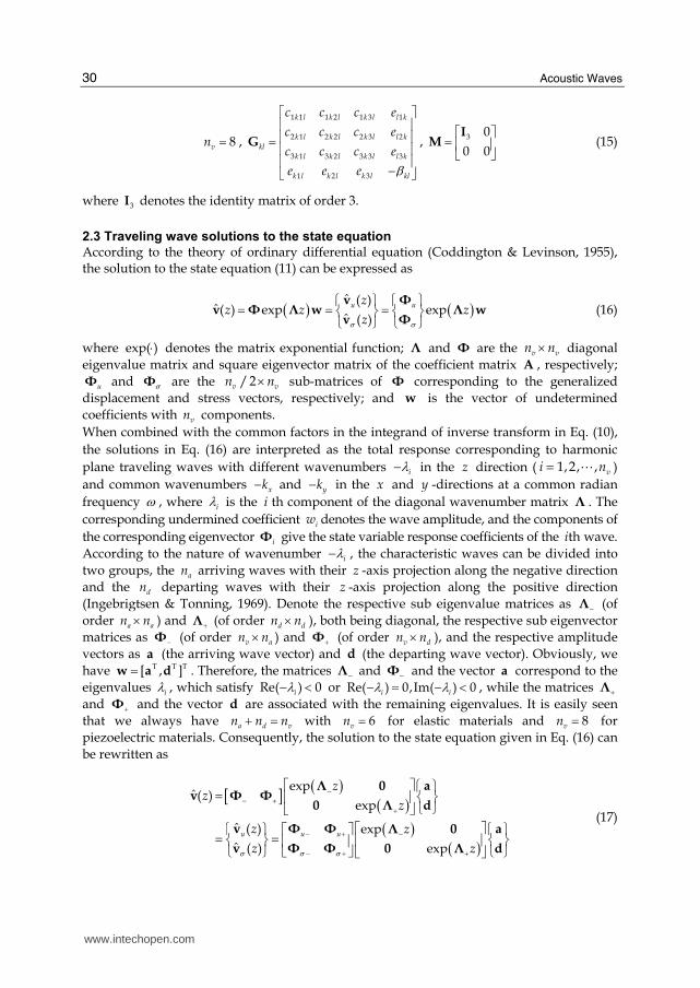
= 8vn ,

β

⎡ ⎤⎢ ⎥⎢ ⎥= ⎢ ⎥⎢ ⎥−⎣ ⎦

1 1 1 2 1 3 1

2 1 2 2 2 3 2

3 1 3 2 3 3 3

1 2 3

k l k l k l l k

k l k l k l l k

kl

k l k l k l l k

k l k l k l kl

c c c e

c c c e

c c c e

e e e

G , ⎡ ⎤= ⎢ ⎥⎣ ⎦

3 0

0 0

IM (15)

where 3I denotes the identity matrix of order 3.

2.3 Traveling wave solutions to the state equation

According to the theory of ordinary differential equation (Coddington & Levinson, 1955), the solution to the state equation (11) can be expressed as

( ) ( )σ σ

⎧ ⎫ ⎧ ⎫= = =⎨ ⎬ ⎨ ⎬⎩ ⎭ ⎩ ⎭ˆ ( )

ˆ ( ) exp expˆ ( )

u uzz z z

z

v Φv Φ Λ w Λ w

v Φ (16)

where ⋅exp( ) denotes the matrix exponential function; Λ and Φ are the ×v vn n diagonal

eigenvalue matrix and square eigenvector matrix of the coefficient matrix A , respectively;

uΦ and σΦ are the ×/2v vn n sub-matrices of Φ corresponding to the generalized

displacement and stress vectors, respectively; and w is the vector of undetermined

coefficients with vn components.

When combined with the common factors in the integrand of inverse transform in Eq. (10),

the solutions in Eq. (16) are interpreted as the total response corresponding to harmonic

plane traveling waves with different wavenumbers λ− i in the z direction ( = A1,2, , vi n )

and common wavenumbers − xk and − yk in the x and y -directions at a common radian

frequency ω , where λi is the i th component of the diagonal wavenumber matrix Λ . The

corresponding undermined coefficient iw denotes the wave amplitude, and the components of

the corresponding eigenvector iΦ give the state variable response coefficients of the thi wave.

According to the nature of wavenumber λ− i , the characteristic waves can be divided into

two groups, the an arriving waves with their z -axis projection along the negative direction

and the dn departing waves with their z -axis projection along the positive direction

(Ingebrigtsen & Tonning, 1969). Denote the respective sub eigenvalue matrices as −Λ (of

order a an n× ) and +Λ (of order d dn n× ), both being diagonal, the respective sub eigenvector

matrices as −Φ (of order v an n× ) and +Φ (of order v dn n× ), and the respective amplitude

vectors as a (the arriving wave vector) and d (the departing wave vector). Obviously, we

have T T T[ , ]=w a d . Therefore, the matrices −Λ and −Φ and the vector a correspond to the

eigenvalues iλ , which satisfy Re( ) 0iλ− < or Re( ) 0,Im( ) 0i iλ λ− = − < , while the matrices +Λ

and +Φ and the vector d are associated with the remaining eigenvalues. It is easily seen

that we always have a d vn n n+ = with 6vn = for elastic materials and 8vn = for

piezoelectric materials. Consequently, the solution to the state equation given in Eq. (16) can

be rewritten as

[ ] ( ) ( )( ) ( )σ σσ

−− +

+− + −− + +

⎡ ⎤ ⎧ ⎫= ⎨ ⎬⎢ ⎥ ⎩ ⎭⎣ ⎦⎡ ⎤⎧ ⎫ ⎧ ⎫⎡ ⎤= =⎨ ⎬ ⎨ ⎬⎢ ⎥⎢ ⎥⎣ ⎦⎩ ⎭ ⎩ ⎭⎣ ⎦

expˆ( )

exp

ˆ ( ) exp

ˆ ( ) expu u u

zz

z

z z

z z

aΛ 0v Φ Φ

d0 Λ

v Φ Φ aΛ 0

Φ Φv d0 Λ

(17)

www.intechopen.com


31

where −uΦ and σ −Φ are ×/ 2v an n sub eigenvector matrices of −Φ corresponding to the

generalized displacement and stress vectors, respectively; +uΦ and σ +Φ are those

×/ 2v dn n sub eigenvector matrices of +Φ . It is noted from Eq. (17) that the only unknowns

in the solutions are the wave amplitudes, which should be determined from the system

equation formulated by simultaneously considering the dynamic state of all constituent

layers of the structure and their interactions. This will be shown in the following section

within the framework of reverberation-ray matrix analysis.

3. Unified formulation of MRRM

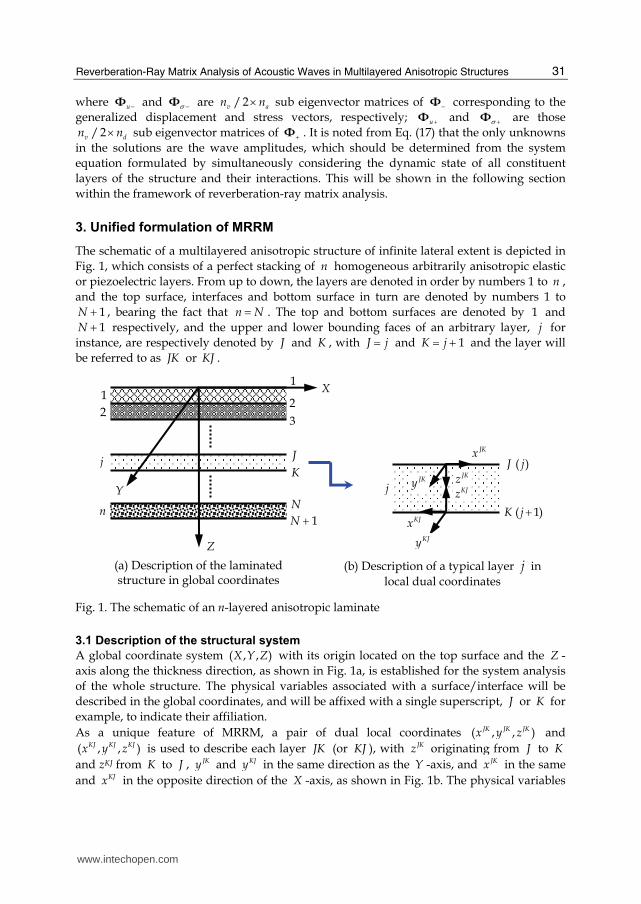
The schematic of a multilayered anisotropic structure of infinite lateral extent is depicted in

Fig. 1, which consists of a perfect stacking of n homogeneous arbitrarily anisotropic elastic

or piezoelectric layers. From up to down, the layers are denoted in order by numbers 1 to n ,

and the top surface, interfaces and bottom surface in turn are denoted by numbers 1 to

+ 1N , bearing the fact that =n N . The top and bottom surfaces are denoted by 1 and

1N + respectively, and the upper and lower bounding faces of an arbitrary layer, j for

instance, are respectively denoted by J and K , with =J j and = + 1K j and the layer will

be referred to as JK or KJ .

Fig. 1. The schematic of an n-layered anisotropic laminate

3.1 Description of the structural system

A global coordinate system ( , , )X Y Z with its origin located on the top surface and the Z -

axis along the thickness direction, as shown in Fig. 1a, is established for the system analysis

of the whole structure. The physical variables associated with a surface/interface will be

described in the global coordinates, and will be affixed with a single superscript, J or K for

example, to indicate their affiliation.

As a unique feature of MRRM, a pair of dual local coordinates ( , , )JK JK JKx y z and

( , , )KJ KJ KJx y z is used to describe each layer JK (or KJ ), with JKz originating from J to K

and zKJ from K to J , JKy and KJy in the same direction as the Y -axis, and JKx in the same

and KJx in the opposite direction of the X -axis, as shown in Fig. 1b. The physical variables

(b) Description of a typical layer j in

local dual coordinates

+ ( 1)K j

JKx ( )J j

jJKzJKyKJz

KJxKJy

11

2

X

Y

Z

2

3

J

Kj

nN

+ 1N

(a) Description of the laminated structure in global coordinates

www.intechopen.com

Acoustic Waves

32

inside the layers will be described in the local dual coordinates and double superscripts, JK

or KJ for instance, will be affixed to any physical quantity to denote the corresponding

coordinate system and the pertaining layer. As an example, ˆ JKv and ˆ KJ

v are the state

vectors for layer JK (or KJ ) in the coordinates ( , , )JK JK JKx y z and ( , , )KJ KJ KJx y z , respectively. To make the sign convection more clear, physical variables are deemed to be positive as it is along the positive direction of the pertinent coordinate axis.

It is seen from Fig. 1b that the dual local coordinates are both right-handed, thus the state

equations in Eq. (11) and the traveling wave solutions in Eqs. (16) and (17) all come into

existence for an arbitrary layer JK (or KJ ) in ( , , )JK JK JKx y z and ( , , )KJ KJ KJx y z , which are

written as

=ˆd ( )ˆ ( )

d

JK JKJK JK JK

JK

zz

z

vA v (18)

=ˆd ( )ˆ ( )

d

KJ KJKJ KJ KJ

KJ

zz

z

vA v (19)

( ) ( )−

− ++

⎡ ⎤ ⎧ ⎫⎪ ⎪⎢ ⎥⎡ ⎤= = ⎨ ⎬⎣ ⎦ ⎢ ⎥ ⎪ ⎪⎩ ⎭⎣ ⎦exp

ˆ ( ) exp( )exp

JK JK JK

JK JK JK JK JK JK JK JK

JKJK JK

zz z

z

Λ 0 av Φ Λ w Φ Φ

d0 Λ (20)

( ) ( )−

− ++

⎡ ⎤ ⎧ ⎫⎪ ⎪⎢ ⎥⎡ ⎤= = ⎨ ⎬⎣ ⎦ ⎢ ⎥ ⎪ ⎪⎩ ⎭⎣ ⎦exp

ˆ ( ) exp( )exp

KJ KJ KJ

KJ KJ KJ KJ KJ KJ KJ KJ

KJKJ KJ

zz z

z

Λ 0 av Φ Λ w Φ Φ

d0 Λ (21)

From Eqs. (20) and (21) we see that there are totally vn N× arriving wave amplitudes and

vn N× departing wave amplitudes for all layers in dual local coordinates, which should be

determined by 2 vn N× relations. It is deduced that the basic unknowns (wave amplitudes)

in the MRRM double in number due to the particular description of dynamic state in dual

local coordinates, as compared with that in other analytical methods which are usually

based on single local coordinates. However, by doing so in the MRRM, the boundary

conditions on surfaces and continuous conditions at interfaces take on an extremely simple

form since the exponential functions in the solutions no longer appear, as will be seen from

Section 3.2. Furthermore, as will be shown in Section 3.3, the arriving and departing wave

amplitudes in dual local coordinates are related directly from the point of view of wave

propagation through the layer. Thus it shall be possible to deduce a system equation in

terms of only the departing wave vectors of all layers. In such a case, the dimension of the

system equation will be the same as the one of other analytical methods based on single

local coordinates, such as the stiffness matrix method and the spectral element method, as

discussed in Section 3.4.

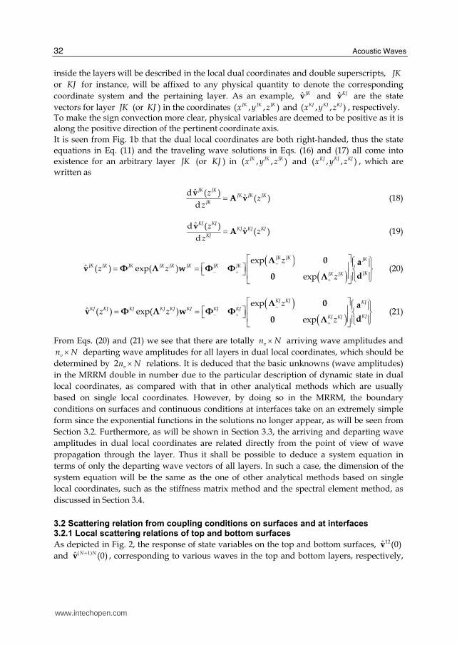
3.2 Scattering relation from coupling conditions on surfaces and at interfaces 3.2.1 Local scattering relations of top and bottom surfaces

As depicted in Fig. 2, the response of state variables on the top and bottom surfaces, 12ˆ (0)v

and ( 1)ˆ (0)N N+v , corresponding to various waves in the top and bottom layers, respectively,

www.intechopen.com


33

should be in accordance with the external state variables 1Êv (= 1 T 1 T Tˆ ˆ[( ) ,( ) ]uE Eσv v ) and ( 1)ˆ N

E+

v

(= ( 1) ( 1)T T Tˆ ˆ[( ) ,( ) ]N NuE Eσ+ +v v ) , i.e.

Fig. 2. The top and bottom surfaces of the multilayered anisotropic structure

12 1ˆ ˆ(0) E E=v T v , ( 1) ( 1)ˆ ˆ(0)N N Nv E E

+ +=T v T v (22)

where ,E uE Eσ=< >T T T is a transformation matrix with /2vuE n=T I and /2vE nσ = −T I ;

,v u σ=< >T T T is also a transformation matrix, with 1,1, 1u =< − − >T and 1, 1,1σ =< − >T for

elastic layers and 1,1, 1, 1u =< − − − >T and 1, 1,1,1σ =< − >T for piezoelectric layers. Here

< ⋅ > denotes the (block) diagonal matrix with elements (or sub-matrices) only on the main

diagonal and /2vnI represents the identity matrix of order / 2vn .

By virtue of Eqs. (20) and (21), the solutions to 12ˆ (0)v and ( 1)ˆ (0)N N+v can be obtained as

12

12 12 12 12 12

12ˆ (0) − +

⎧ ⎫⎪ ⎪⎡ ⎤= = ⎨ ⎬⎣ ⎦ ⎪ ⎪⎩ ⎭a

v Φ w Φ Φd

(23)

( 1)

( 1) ( 1) ( 1) ( 1) ( 1)

( 1)ˆ (0)

N N

N N N N N N N N N N

N N

++ + + + +− + +

⎧ ⎫⎪ ⎪⎡ ⎤= = ⎨ ⎬⎣ ⎦ ⎪ ⎪⎩ ⎭a

v Φ w Φ Φd

(24)

where the exponential functions disappear since the thickness coordinates on the surfaces

are always zero in the corresponding local coordinates. This is the main advantage of

introducing the dual local coordinates. It should be noticed that half of the components of

vectors 1Êv and ( 1)ˆ N

E+

v are known, which are denoted by vectors 1ˆKv and ( 1)ˆ N

K+

v , respectively,

while the remaining half are unknown, denoted by vectors 1Ûv and ( 1)ˆ N

U+

v , respectively.

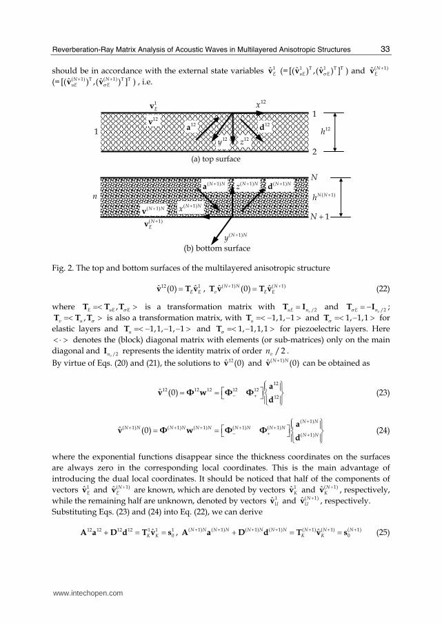
Substituting Eqs. (23) and (24) into Eq. (22), we can derive

12 12 12 12 1 1 10

ˆK K+ = =A a D d T v s , ( 1) ( 1) ( 1) ( 1) ( 1) ( 1) ( 1)

0ˆN N N N N N N N N N N

K K+ + + + + + ++ = =A a D d T v s (25)

N( 1)N N+d

( 1)N N+a

( 1)N Nz +

( 1)N Nx +( 1)N Nh +n

1N +( 1)N Ny +

2

1

12z

12h12y

12d

12x

12a

1

(a) top surface

(b) bottom surface

12v

1Ev

( 1)N N+v

( 1)NE

+v

www.intechopen.com

Acoustic Waves

34

where 12A , 12

D , ( 1)N N+A , ( 1)N N+

D , 1KT ( ( 1)N

K+

T ) are the coefficient matrices with components

extracted, in accordance with 1ˆKv and ( 1)ˆ N

K+

v , from 12−Φ , 12+Φ , ( 1)N N+−Φ , ( 1)N N++Φ and ET ( ET

and vT ) respectively. 10s and ( 1)

0N+s are excitation source vectors with / 2vn components of

the top and bottom surfaces, respectively. Particularly as far as free waves are concerned, if

the top surface is mechanically traction-free (and electrically open-circuit), we have

1 1 1 1 1 Tˆ ˆ ˆ ˆ ˆ[ , , ]K E X Y Zσ τ τ σ= = =v v 0 (or 1 1 1 1 1 1 Tˆˆ ˆ ˆ ˆ ˆ[ , , , ]K E X Y Z ZDσ τ τ σ= = =v v 0 ) (26)

12 12σ −=A Φ , 12 12σ +=D Φ (27)

and when the top surface is mechanically fixed (and electrically closed-circuit) we have

1 1 1 1 1 Tˆ ˆ ˆ ˆ ˆ[ , , ]K uE X Y Zu u u= = =v v 0 (or 1 1 1 1 1 1 Tˆ ˆ ˆ ˆ ˆ ˆ[ , , , ]K uE X Y Z Zu u u ϕ= = =v v 0 ) (28)

12 12u−=A Φ , 12 12

u+=D Φ (29)

For mixed boundary conditions, the form of known quantities and coefficient matrices can

also be worked out accordingly. The boundary conditions on the bottom surface can be

similarly deduced and will not be discussed for brevity.

Eq. (25) can be further written in a form of local scattering relations on the top and bottom

surfaces

1 1 1 1 10+ =A a D d s , ( 1)1 1 1 1

0NN N N N ++ + + ++ =A a D d s (30)

where 1 12=a a ( ( 1)1 N NN ++ =a a ) and 1 12=d d ( ( 1)1 N NN ++ =d d ) are the arriving and departing

wave vectors of the top (bottom) surface, 1 12=A A ( ( 1)1 N NN ++ =A A ) and 1 12=D D

( ( 1)1 N NN ++ =D D ) are 12/2v an n× ( ( 1)/2 N Nv an n +× ) and 12/2v dn n× ( ( 1)/2 N N

v dn n +× ) coefficient

matrices corresponding to the arriving and departing wave vectors of the top (bottom)

surface, respectively. It should be pointed out that the form of local scattering relations at the boundaries given in Eq. (30) is also valid for surface waves in a multilayered structure.

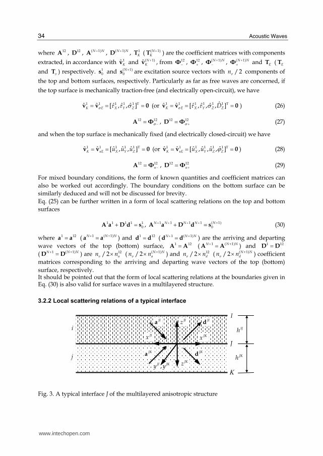
3.2.2 Local scattering relations of a typical interface

Fig. 3. A typical interface J of the multilayered anisotropic structure

K

J

JKz

JKh

,JI JKy y

JKd

JKx

JKa

IJId

JIa

JIz

JIx

IJh

j

i

www.intechopen.com


35

Since the adjacent layers in the structure are perfectly bonded, the state variables should be continuous across the interfaces. Taking the typical interface J as shown in Fig. 2 for illustration, the compatibility of the generalized displacements and equilibrium of the generalized forces require

ˆ ˆ(0) (0)JI JKv =T v v (31)

This gives, according to the solutions in Eqs. (20) and (21),

JI JI JI JK JK JK

u u u u u u

JI JI JI JK JK JKσ σ σ σ σ σ− + − +− + − +

⎡ ⎤ ⎧ ⎫ ⎡ ⎤ ⎧ ⎫⎪ ⎪ ⎪ ⎪=⎨ ⎬ ⎨ ⎬⎢ ⎥ ⎢ ⎥⎪ ⎪ ⎪ ⎪⎣ ⎦ ⎩ ⎭ ⎣ ⎦ ⎩ ⎭TΦ TΦ a Φ Φ a

T Φ T Φ d Φ Φ d (32)

It should be noticed once again that there is no exponential functions in the coupling

equation (32) for interfaces. By grouping the arriving and departing wave vectors of relevant

layers into the local arriving and departing wave vectors of the interface T T T[( ) ,( ) ]J JI JK=a a a

and T T T[( ) ,( ) ]J JI JK=d d d , Eq. (32) is reduced to the local scattering relation of the typical

interface J

J J J J+ =A a D d 0 (33)

where the ( )JI JKv a an n n× + and ( )JI JK

v d dn n n× + coefficient matrices JA and J

D , respectively, are

JI JK

J u u u

JI JKσ σ σ− −− −

⎡ ⎤−= ⎢ ⎥−⎣ ⎦TΦ Φ

AT Φ Φ

, JI JK

J u u u

JI JKσ σ σ+ ++ +

⎡ ⎤−= ⎢ ⎥−⎣ ⎦T Φ Φ

DT Φ Φ

(34)

There are altogether N – 1 (n – 1) interfaces in the multilayered structure, so that we have 1N − ( 1n − ) local scattering equations like Eq. (33).

3.2.3 Global scattering relation of the structure

The local scattering relations of top surface, interfaces and bottom surface have respectively

/ 2vn , ( 1)vn N× − and / 2vn equations, which are grouped together from up to down to

give the vn N× global scattering relation

0+ =Aa Dd s (35)

where the global arriving and departing wave vectors a and d are

T( 1) ( 1)12 T 21 T 23 T T T T T( ) ,( ) ,( ) , ,( ) ,( ) , ,( ) ,( )N N N NJI JK + +⎡ ⎤= ⎣ ⎦a a a a a a a aA A

T( 1) ( 1)12 T 21 T 23 T T T T T( ) ,( ) ,( ) , ,( ) ,( ) , ,( ) ,( )N N N NJI JK + +⎡ ⎤= ⎣ ⎦d d d d d d d dA A (36)

the corresponding ( ) ( )v vn N n N× × × coefficient matrices A and D are

1 2 1, , , , ,J N +=< >A A A A AA A , 1 2 1, , , , ,J N +=< >D D D D DA A (37)

and T( 1)1 T T T T

0 0 0( ) , , , ,( )N +⎡ ⎤= ⎣ ⎦s s 0 0 sA is the global excitation source vector. It should be noted

that the forming process of scattering relations in Eqs. (30), (33) and (35) exclude matrix inversion as compared to that in the original formulation of MRRM (Pao et al, 2000, 2007; Su

www.intechopen.com

Acoustic Waves

36

et al., 2002; Tian et al., 2006), which guarantees the numerical stability and at the same time enables the inclusion of surface and interface wave modes, in the proposed formulation of MRRM (Guo & Chen, 2008a, 2008b; Guo, 2008; Guo et al., 2009).

3.3 Phase relation from compatibility conditions of layers 3.3.1 Local phase relation of a typical layer Considering the formation of the dual local coordinates of a typical layer JK (KJ) as discussed in Section 3.1, we have the geometrical dual transformation relations

JK KJx x= − , JK KJy y= , JK JK KJz h z= − , d dJK KJz z= − (38)

where JKh ( KJh= ) represents the thickness of layer JK (KJ), and the physical dual transformation relations

( ) ( )ˆ ˆJK JK KJ KJvz z=v T v (39)

By virtue of Eqs. (18) and (19), Eqs. (38) and (39), and the definitions of eigenvalue and eigenvector, it is derived that

1( ) ( )KJ KJ JK JKv vz z −= −A T A T , JK KJ= −Λ Λ , JK KJ

v=Φ TΦ (40)

It is interpreted that if JKλ and JKλφ are the eigenvalue and eigenvector of the coefficient matrix JK

A , then JKλ− and JKv λT φ must be the corresponding eigenvalue and eigenvector of

the coefficient matrix KJA . The equality relations between the numbers of arriving and

departing waves in dual local coordinates, i.e. JK KJa dn n= and JK KJ

d an n= , are also implied. Substituting Eqs. (20) and (21) into Eq. (39), and in view of Eq. (40) and 1 ,v v

−=T T one obtains the local phase relation of a typical layer JK (KJ)

( ) ( )

exp

exp

JK JKJK KJ JKJK JKa

KJ JKKJ JK KJJK JKd

h

h

−

+

⎡ ⎤−⎧ ⎫ ⎧ ⎫ ⎧ ⎫⎡ ⎤ ⎡ ⎤⎪ ⎪ ⎪ ⎪ ⎪ ⎪⎢ ⎥= =⎨ ⎬ ⎨ ⎬ ⎨ ⎬⎢ ⎥ ⎢ ⎥⎢ ⎥⎪ ⎪ ⎪ ⎪ ⎪ ⎪⎣ ⎦ ⎣ ⎦⎩ ⎭ ⎩ ⎭ ⎩ ⎭⎣ ⎦Λ 0a d dP 0 0 I

0 P I 0a d d0 Λ (41)

where the JK JKa an n× and JK JK

d dn n× diagonal matrices exp( )JK JK JKh−= −P Λ and exp( )KJ JK JKh+=P Λ are referred to as local phase matrices, and JK

aI and JKdI are identity

matrices of order JKan and JK

dn , respectively. It should be noted that the exponentially growing functions, which usually cause numerical instability (such as in the TMM) for large values of the frequency-thickness product, have been completely excluded from the phase matrices JK

P and KJP , since we always have Re( ) 0JK JKhλ− > or

Re( ) 0, Im( ) 0JK JK JK JKh hλ λ− −= > ( Re( ) 0JK JKhλ+ < or Re( ) 0, Im( ) 0JK JK JK JKh hλ λ+ += < ). As indicated by Eq. (41), there are vn equations in the local phase relation of each layer.

3.3.2 Global phase relation of the structure

Grouping together the local phase relations for all layers from up to down yields the global phase relation with vn N× equations

= =a Pd PUd (42)

where the ( ) ( )v vn N n N× × × block diagonal matrices P , named the global phase matrix, is composed of

www.intechopen.com


37

( 1) ( 1)12 21 23, , , , , , , ,N N N NJI JK + +=< >P P P P P P P PA A (43)

the variant of the global departing wave vector d is related to the wave vector d by the ( ) ( )v vn N n N× × × block diagonal matrix U , which is referred to as the global permutation matrix, to account for the different sequence of components arrangement between d and d . The specific forms of U and d are as follows

( 1)12 23, , , , , N NJK +=< >U U U U UA A , v v

JKJK an n JK

d

×⎡ ⎤= ⎢ ⎥⎣ ⎦0 I

UI 0

(44)

T( 1) ( 1)21 T 12 T 32 T T T T T( ) ,( ) ,( ) , ,( ) ,( ) , ,( ) ,( )N N N NIJ KJ + +⎡ ⎤= ⎣ ⎦d d d d d d d dA A (45)

It is seen from Eq. (42) that the global arriving and departing wave vectors a and d, consisting of respectively the arriving and departing wave amplitudes in local dual coordinates of all layers and having the same forms as those in the global scattering relation in Eq. (36), are related directly through the global phase relation, which enables the dimension reduction of the system equation, making the final scale the same as the one in other analytical methods which are based on single local coordinates.

3.4 System equation and dispersion equation

The global scattering relation in Eq. (35) and global phase relation in Eq. (42) contain

respectively vn N× equations for the vn N× unknown arriving wave amplitudes (in a )

and vn N× unknown departing wave amplitudes (in d ). Thus the wave vectors can be

determined. Substitution of Eq. (42) into Eq. (35) gives the system equation

0( )+ = =APU D d Rd s (46)

where = +R APU D is the system matrix. If there is no surface excitation, i.e. s0 = 0 and the free wave propagation problem is considered, the vanishing of the system matrix determinant yields the following dispersion equation

( ; ; )x yk k ω =R 0 (47)

which may be solved numerically by a proper root searching technique (Guo, 2008). Thus, the complete dispersion curves of various waves can be obtained, as illustrated in Section 4 for multilayered anisotropic elastic structures. If there is surface excitation, from Eq. (46) we have

1 10 0( )− −= + =d APU D s R s (48)

Further making use of the global phase relation (42), the solution of the state vector in Eq. (20) and the inverse Fourier transform in Eq. (10) with respect to the wavenumbers, the steady-state response of state variables of a layer at circular frequency ω can be expressed as

{ }i( )

2

i( )102

1ˆ ˆ( , , ; ) ( ; , ; )e d d

(2 )

1exp( ) exp( ) e d d

(2 )

JK JKx y

JK JKx y

k x k yJK JK JK JK JK JKx y x y

k x k yJK JK JK KJ JK JK JK JKx y

x y z k k z k k

z z k k

ω ωππ

+∞ +∞ +−∞ −∞

+∞ +∞ +−− − + +−∞ −∞

== +

∫ ∫∫ ∫

v v

Φ Λ E Φ Λ E R s

(49)

www.intechopen.com

Acoustic Waves

38

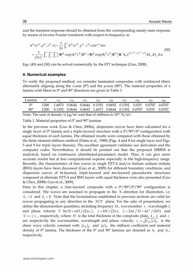
and the transient response should be obtained from the corresponding steady-state response by means of inverse Fourier transform with respect to frequency as

{ }i

i( )103

1ˆ( , , , ) ( , , ; )e d

21

exp( ) exp( ) e d d d(2 )

JK JKx y

JK JK JK JK JK JK JK JK t

k x k y tJK JK JK KJ JK JK JK JKx y

x y z t x y z

z z k k

ω

ω

ω ωπωπ

+∞−∞

+∞ +∞ +∞ + +−− − + +−∞ −∞ −∞

== +

∫∫ ∫ ∫

v v

Φ Λ E Φ Λ E R s

(50)

Eqs. (49) and (50) can be solved numerically by the FFT technique (Guo, 2008).

4. Numerical examples

To verify the proposed method, we consider laminated composites with reinforced fibers alternately aligning along the x-axis (0°) and the y-axis (90°). The material properties of a lamina with fibers in 0° and 90° directions are given in Table 1.

Lamina ρ c11 c12 c13 c22 c23 c33 c44 c55 c66

0° 1200 1.6073 0.0644 0.0644 0.1392 0.0692 0.1392 0.035 0.0707 0.0707 90° 1200 0.1392 0.0644 0.0692 1.6073 0.0644 0.1392 0.0707 0.035 0.0707

Note: The unit of density is kg/m3 and that of stiffness is 1011 N/m2.

Table 1. Material properties of 0° and 90° laminas

In the previous work (Guo & Chen, 2008a), dispersion curves have been calculated for a

single layer of 0° lamina and a triple-layered structure with a 0°/90°/0° configuration with

equal thickness of each lamina. The obtained results were compared with those obtained by

the finite element stiffness method (Datta et al., 1988) (Figs. 4 and 8 for single layer and Figs.

5 and 9 for triple layers therein). The excellent agreement validates our derivation and the

computer codes. Nevertheless, it should be pointed out that the proposed MRRM is

analytical, based on continuous (distributed-parameter) model. Thus, it can give more

accurate results but at less computational expense especially in the high-frequency range.

Recently, the characteristics of free waves in single PZT-4 and/or barium sodium niobate

(BSN) layers have been discussed (Guo et al., 2009) for different boundary conditions, and

dispersion curves of bi-layered, triple-layered and ten-layered piezoelectric structures

composed of alternate PZT-4 and BSN layers with equal thickness were also presented (Guo

& Chen, 2008b; Guo et al., 2009).

Here in this chapter, a four-layered composite with a 0°/90°/0°/90° configuration is

considered. The waves are assumed to propagate in the X -direction for illustration, i.e.

xk k= and 0yk = . Note that the formulations established in previous sections are valid for

waves propagating in any direction in the XOY plane. For the sake of presentation, we

define the dimensionless quantities, including frequency Ω , wavenumber γ , wavelength L

and phase velocity V by /(2 )sH cω πΩ = , /(2 )kHγ π= , 22 / 4 /( )L H kHπλ π= = and

/ sV c c= , respectively, where H is the total thickness of the composite plate, k , λ and c

are respectively the wavenumber, wavelength and phase velocity, 55 0( )sc c ρ °= is the

shear wave velocity constant with 55 0( )c ° and 0( )ρ ° the stiffness coefficient and material

density of 0° lamina. The thickness of the 0° and 90° laminas are denoted as 1h and 2h ,

respectively.

www.intechopen.com


39

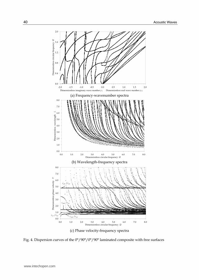
4.1 Dispersion curves of multilayered anisotropic structures with free surfaces

First, the laminas of the four-layered composite structure are assumed to have equal thicknesses and the top and bottom surfaces of the composite are assumed to be traction-free. The dispersion curves, in terms of frequency-wavenumber spectra, wavelength-frequency spectra and phase velocity-frequency spectra, are presented in Figs. 4(a), 4(b) and 4(c) respectively. The sub-figures (a) to (c) in Fig. 4 show similar dispersion properties of free waves in the four-layered composite as compared with those for single and triple layers. The quasi P-SV and SH bulk modes, surface and interface modes and characteristic asymptotic line are obtained all at once from the dispersion equation by a root searching algorithm.

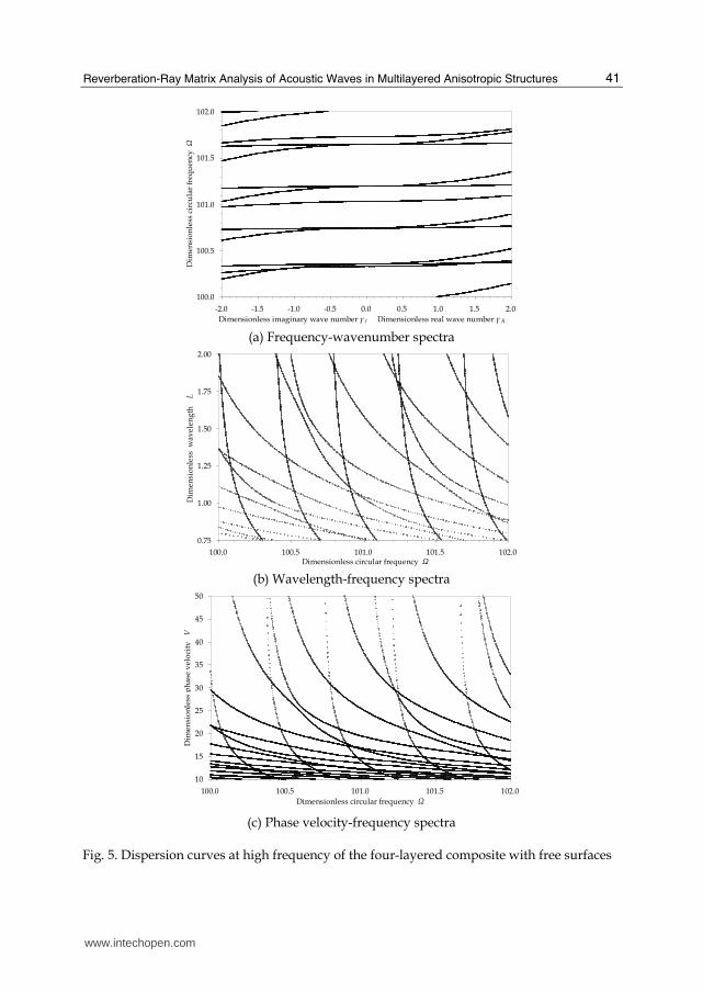
4.2 Dispersion curves in high frequency range

The frequency-wavenumber, wavelength-frequency and phase velocity-frequency spectra

with dimensionless frequency Ω in the range of 100 to 102 are given in Figs. 5(a), 5(b) and 5(c) respectively, which indicate the proposed formulation of MRRM can assure a good numerical stability in the high-frequency range. Since the wave modes at small values of wavelength and phase velocity are relatively intensive and difficult to differentiate within this frequency range, as implied in Figs. 4(b) and 4(c), the dimensionless wavelength L and phase velocity V are specified within 0.75~2.00 and 10~50 in Figs. 5(b) and 5(c), respectively.

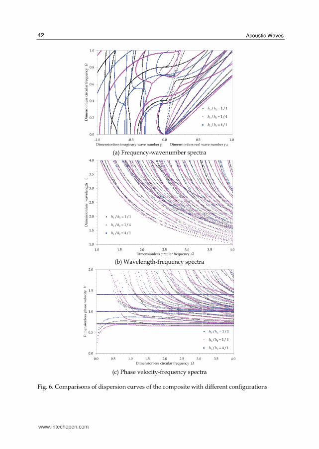
4.3 Effects of configuration on the dispersion curves

Next, the thickness of the 0° and 90° laminas of the four-layered composite are assumed to

be unequal in order to study the effect of configuration on the characteristics of free waves.

The dispersion curves for cases 1 2/ 1 / 4h h = and 1 2/ 4 /1h h = as well as their comparison

with those for the equal thickness case (denoted as 1 2/ 1 /1h h = ) are depicted in Fig. 6, with

the frequency-wavenumber, wavelength-frequency and phase velocity-frequency spectra

given in the sub-figures (a), (b) and (c) respectively.

It is seen from Fig. 6 that the dispersion curves of a specified wave mode corresponding to

the case 1 2/ 1 /1h h = locate in between those for cases 1 2/ 1 / 4h h = and 1 2/ 4 /1h h = . As

also indicated in Fig. 6, the thickness ratio has a distinct effect on the characteristics of all

free wave modes. The effect is however somehow larger for the higher-order wave modes

than the lower-order ones.

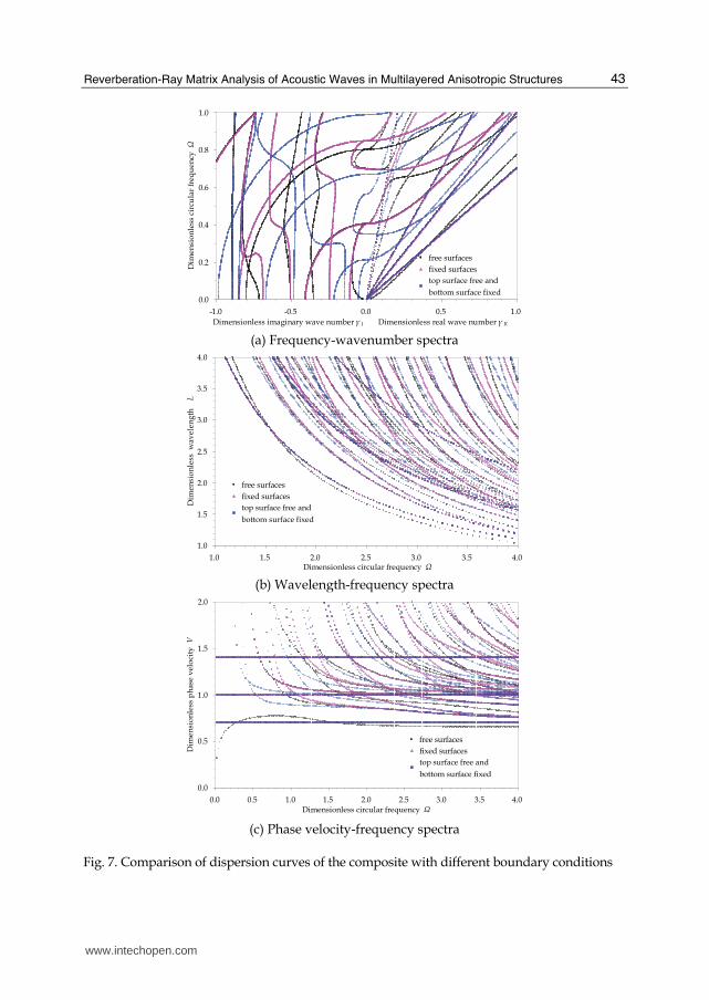
4.4 Effects of boundary conditions on the dispersion curves

In order to show the effects of boundary conditions on the dispersion characteristics, the same 0°/90°/0°/90° laminated composite with equal layer thicknesses is considered for two different boundary conditions: one is that both the top and bottom surfaces are fixed and the other is that the top surface is traction-free while the bottom surface is fixed. The dispersion curves for the two cases are given in Fig. 7 and compared with those for a laminate with free surfaces. It is seen from Fig. 7 that some parts of the dispersion curves of certain specified modes for

the four-layered composite with different surface conditions may coincide, but they may be

completely different at other parts or for other modes. Fig. 7 indicates that the boundary

conditions have a complex effect on the dispersion characteristics of free waves in

multilayered anisotropic structures. In-depth study is needed.

www.intechopen.com

Acoustic Waves

40

0.0

0.4

0.8

1.2

1.6

2.0

-2.0 -1.5 -1.0 -0.5 0.0 0.5 1.0 1.5 2.0

Dimensionless imaginary wave number γ I

Dim

ensi

on

less

cir

cula

r fr

equ

ency

Ω

Dimensionless real wave number γ R (a) Frequency-wavenumber spectra

0.0

1.0

2.0

3.0

4.0

5.0

6.0

7.0

8.0

0.0 1.0 2.0 3.0 4.0 5.0 6.0 7.0 8.0Dimensionless circular frequency Ω

Dim

ensi

on

less

wav

elen

gth

L

(b) Wavelength-frequency spectra

0.0

1.0

2.0

3.0

4.0

5.0

6.0

7.0

8.0

0.0 1.0 2.0 3.0 4.0 5.0 6.0 7.0 8.0

Dim

ensi

on

less

ph

ase

vel

oci

ty

V

Dimensionless circular frequency Ω

90 0/p sc c° °

90 0/s sc c° °0 0/s sc c° °

0 0/p sc c° °

(c) Phase velocity-frequency spectra

Fig. 4. Dispersion curves of the 0°/90°/0°/90° laminated composite with free surfaces

www.intechopen.com


41

100.0

100.5

101.0

101.5

102.0

-2.0 -1.5 -1.0 -0.5 0.0 0.5 1.0 1.5 2.0

Dim

ensi

on

less

cir

cula

r fr

equ

ency

Ω

Dimensionless imaginary wave number γ I Dimensionless real wave number γ R (a) Frequency-wavenumber spectra

0.75

1.00

1.25

1.50

1.75

2.00

100.0 100.5 101.0 101.5 102.0Dimensionless circular frequency Ω

Dim

ensi

on

less

wav

elen

gth

L


10

15

20

25

30

35

40

45

50

100.0 100.5 101.0 101.5 102.0

Dim

ensi

on

less

ph

ase

vel

oci

ty

V


(c) Phase velocity-frequency spectra Fig. 5. Dispersion curves at high frequency of the four-layered composite with free surfaces

www.intechopen.com

Acoustic Waves

42

0.0

0.2

0.4

0.6

0.8

1.0

-1.0 -0.5 0.0 0.5 1.0

Dim

ensi

on

less

cir

cula

r fr

equ

ency

Ω

Dimensionless imaginary wave number γ I Dimensionless real wave number γ R

1 2/ 1 /1h h =

1 2/ 4 /1h h =1 2/ 1 /4h h =

(a) Frequency-wavenumber spectra

1.0

1.5

2.0

2.5

3.0

3.5

4.0

1.0 1.5 2.0 2.5 3.0 3.5 4.0Dimensionless circular frequency Ω

Dim

ensi

on

less

wav

elen

gth

L

1 2/ 1/1h h =

1 2/ 4 /1h h =1 2/ 1/4h h =


0.0

0.5

1.0

1.5

2.0

0.0 0.5 1.0 1.5 2.0 2.5 3.0 3.5 4.0

Dim

ensi

on

less

ph

ase

vel

oci

ty V


1 2/ 1 /1h h =

1 2/ 4 /1h h =1 2/ 1/4h h =


Fig. 6. Comparisons of dispersion curves of the composite with different configurations

www.intechopen.com


43

0.0

0.2

0.4

0.6

0.8

1.0

-1.0 -0.5 0.0 0.5 1.0

Dim

ensi

on

less

cir

cula

r fr

equ

ency

Ω

Dimensionless imaginary wave number γ I Dimensionless real wave number γ R

free surfaces

top surface free and

bottom surface fixed

fixed surfaces

(a) Frequency-wavenumber spectra

1.0

1.5

2.0

2.5

3.0

3.5

4.0

1.0 1.5 2.0 2.5 3.0 3.5 4.0Dimensionless circular frequency Ω

Dim

ensi

on

less

wav

elen

gth

L

free surfaces



fixed surfaces


0.0

0.5

1.0

1.5

2.0

0.0 0.5 1.0 1.5 2.0 2.5 3.0 3.5 4.0

Dim

ensi

on

less

ph

ase

vel

oci

ty V


free surfaces



fixed surfaces


Fig. 7. Comparison of dispersion curves of the composite with different boundary conditions

www.intechopen.com

Acoustic Waves

44

5. Conclusion

We present a unified formulation of the method of reverberation-ray matrix (MRRM) for the analysis of acoustic wave propagation in multilayered anisotropic elastic/piezoelectric structures based on the state space formalism and Fourier transforms in the framework of three-dimensional elasticity or piezoelectricity. The proposed formulation of MRRM includes all wave modes in the structure and possesses good numerical stability by properly excluding exponentially growing function and matrix inversion operation. It is therefore suitable for the accurate analysis of acoustic waves in complex multilayered anisotropic structures by a uniform computer program. In comparison with the well-known traditional transfer matrix method, the present MRRM is unconditionally numerically stable, irrespective of the total number of layers, the thickness of individual layers and the frequency. Besides, in comparison with the numerical methods based on discrete models, the present MRRM is based on a continuous model (distributed-parameter model) and gives accurate results at a much smaller computational cost especially in the high-frequency range. Numerical results indicate a high accuracy and broad versatility of the proposed formulation of MRRM for wave propagation in multilayered anisotropic structures with various configurations and boundary conditions in any frequency range. The obtained dispersion curves and their dependence on the structural configurations and boundary conditions shall be useful in the design and optimization of laminated composites and acoustic wave devices.

6. Acknowledgements

This study was financially supported by the National Natural Science Foundation of China (No. 10902045 and No. 10725210) and the Postdoctoral Science Foundation of China (No. 20090460155) and the Fundamental Research Funds for the Central Universities of China.

7. References

Achenbach, J. D. (1973). Wave Propagation in Elastic Solids, North-Holland, Amsterdam. Coddington, E. A., Levinson, N. (1955). Theory of Ordinary Differential Equations, McGraw-

Hill, New York. Adler, E. L. (1990). Matrix methods applied to acoustic waves in multilayers, IEEE

Transactions on Ultrasonics, Ferroelectrics, and Frequency Control, 37(6): 485-490. Adler, E. L. (2000). Bulk and surface acoustic waves in anisotropic solids, International

Journal of High Speed Electronics and Systems, 10(3): 653-684. Alshits V. I. & Maugin, G. A. (2008). Dynamics of anisotropic multilayers, Wave Motion,

45(5): 629-640. Auld, B. A. (1990). Acoustic Fields and Waves in Solids, Second Edition, Vol. I & II, Robert E.

Krieger Publishing Company, Malabar, Florida. Brekhovskikh, L. M. (1980). Waves in Layered Media, Second Edition. Academic Press, New York. Chakraborty, A. & Gopalakrishnan, S. (2006). A spectral finite element model for wave

propagation analysis in laminated composite plate, ASME Journal of Vibration and Acoustics, 128: 477-488.

Chimenti, D. E. (1997). Guided waves in plates and their use in materials characterization, Applied Mechanics Reviews, 50(5): 247-284.

Collet, B. (2004). Recursive surface impedance matrix methods for ultrasonic wave propagation in piezoelectric multilayers, Ultrasonics, 42: 189-197.

Datta, S. K., Shah, A. H., Bratton, R. L. & Chakraborty, T. (1988). Wave propagation in laminated composite plates, Journal of the Acoustical Society of America, 83(6): 2020-2026.

www.intechopen.com


45

Degettekin, F. L., Honein, B. V., & Khuri-Yakub, B. T. (1996). Application of surface impedance approach to ultrasonic wave propagation in layered anisotropic media, IEEE Ultrasonics Symposium, 559-562.

Ding, H. J. & Chen, W. Q. (2001). Three Dimensional Problems of Piezoelasticity. Nova Science Publishers, New York.

Ewing, W. M., Jardetzky, W. S. & Press, F. (1957). Elastic Waves in Layered Media. McGraw-Hill, New York.

Fedosov, V. I., Aniiimkin, V. I., Kotelyanskii, I. M., Caliendo, C., Verardi, P. & Verona, E. (1996). Analysis of acoustic waves in multilayers using compound matrices, IEEE Ultrasonics Symposium, 207-212.

Guo, Y. Q. (2008). The Method of Reverberation-Ray Matrix and its Applications, Doctorial dissertation. Zhejiang University, Hangzhou, China. (in Chinese)

Guo, Y. Q. & Chen, W. Q. (2008a). On free wave propagation in anisotropic layered media, Acta Mechanica Solida Sinica, 21(6): 500-506.

Guo, Y. Q. & Chen, W. Q. (2008b) Modeling of multilayered acoustic wave devices with the method of reverberation-ray matrix, 2008 Symposium on Piezoelectricity, Acoustic Waves, and Device Applications (SPAWDA 2008), 105-110.

Guo, Y. Q., Chen, W. Q. & Zhang, Y. L. (2009). Guided wave propagation in multilayered piezoelectric structures, Science in China, Series G: Physics, Mechanics and Astronomy, 52(7): 1094-1104.

Haskell, N. A. (1953). The dispersion of surface waves on multilayered media, Bulletin of the Seismological Society of America, 43: 17-34.

Honein, B., Braga, A. M. B., Barbone, P. & Herrmann, G. (1991). Wave propagation in piezoelectric layered media with some applications, Journal of Intelligent Material Systems and Structures, 2: 542-557.

Hosten, B. & Castaings, M. (2003). Surface impedance matrices to model the propagation in multilayered media, Ultrasonics, 41: 501-507.

Igel, H., Mora, P. & Riollet, B. (1995). Anisotropic wave propagation through finite-difference grids, Geophysics, 60(4): 1203-1216.

Ingebrigtsen, K. A. & Tonning, A. (1969). Elastic surface waves in crystal, Physical Review, 184: 942-951.

Kausel, E. & Roesset, J. M. (1981). Stiffness matrices for layered soils, Bulletin of the Seismological Society of America, 71: 1743-1761.

Kennett, B. L. N. (1983). Seismic Wave Propagation in Stratified Media, Cambridge University Press, Cambridge.

Lowe, M. J. S. (1995). Matrix techniques for modeling ultrasonic waves in multilayered media, IEEE Transactions on Ultrasonics, Ferroelectrics, and Frequency Control, 42: 525-542.

Makkonen, T. (2005). Numerical Simulations of Microacoustic Resonators and Filters, Doctoral Dissertation. Helsinki University of Technology, Espoo, Finland.

Nayfeh, A. H. (1995). Wave Propagation in Layered Anisotropic Media with Applications to Composites. Elsevier, Amsterdam.

Pao, Y. H., Chen, W. Q. & Su, X. Y. (2007). The reverberation-ray matrix and transfer matrix analyses of unidirectional wave motion, Wave Motion, 44: 419-438.

Pao, Y. H., Su, X. Y. & Tian, J. Y. (2000). Reverberation matrix method for propagation of sound in a multilayered liquid, Journal of Sound and Vibration, 230(4): 743-760.

Pastureaud, T., Laude, V. & Ballandras S. (2002). Stable scattering-matrix method for surface acoustic waves in piezoelectric multilayers, Applied Physics Letters, 80: 2544-2546.

Rizzi, S. A. & Doyle, J. F. (1992). A spectral element approach to wave motion in layered solids, ASME Journal of Vibration and Acoustics, 114: 569-577.

www.intechopen.com

Acoustic Waves

46

Rokhlin, S. I. & Wang, L. (2002a). Stable recursive algorithm for elastic wave propagation in layered anisotropic media: Stiffness matrix method, Journal of the Acoustical Society of America, 112: 822-834.

Rokhlin, S. I. & Wang, L. (2002b). Ultrasonic waves in layered anisotropic media: characterization of multidirectional composites, International Journal of Solids and Structures, 39(16): 4133-4149.

Rose, J. L. (1999). Ultrasonic Waves in Solid Media, Cambridge University Press, Cambridge. Shen, S. P., Kuang, Z. B. & Hu, S.L. (1998). Wave propagation in multilayered anisotropic

media, Mechanics Research Communications, 25(5): 503-507. Stroh, A. N. (1962). Steady state problems in anisotropic elasticity, Journal of Mathematics and

Physics, 41: 77-103. Su, X. Y., Tian, J. Y. & Pao, Y. H. (2002). Application of the reverberation-ray matrix to the

propagation of elastic waves in a layered solid, International Journal of Solids and Structures, 39: 5447-5463.

Synge, J. L. (1956). Flux of energy for elastic waves in anisotropic media, Proceedings of the Royal Irish Academy, 58: 13-21.

Tan, E. L. (2005). Stiffness matrix method with improved efficiency for elastic wave propagation in layered anisotropic media, Journal of the Acoustical Society of America, 118(6): 3400-3403.

Tan, E. L. (2006). Hybrid compliance-stiffness matrix method for stable analysis of elastic wave propagation in multilayered anisotropic media, Journal of the Acoustical Society of America, 119(1): 45-53.

Tan, E. L. (2007). Matrix Algorithms for modeling acoustic waves in piezoelectric multilayers, IEEE Transactions on Ultrasonics, Ferroelectrics, and Frequency Control, 54: 2016-2023.

Tarn, J. Q. (2002a). A state space formalism for anisotropic elasticity. Part I: Rectilinear anisotropy, International Journal of Solids and Structures, 39: 5143-5155

Tarn, J. Q. (2002b). A state space formalism for piezothermoelasticity, International Journal of Solids and Structures, 39: 5173-5184

Thomson, T. (1950). Transmission of elastic waves through a stratified solid medium, Journal of Applied Physics, 21: 89-93.

Tian, J. Y., Yang, W. X. & Su, X. Y. (2006). Transient elastic waves in a transversely isotropic laminate impacted by axisymmetric load, Journal of Sound and Vibration, 289: 94-108.

Wang, L. & Rokhlin, S. I. (2001). Stable reformulation of transfer matrix method for wave propagation in layered anisotropic media, Ultrasonics, 39: 413-424.

Wang, L. & Rokhlin, S. I. (2002a). An efficient stable recursive algorithm for elastic wave propagation in layered anisotropic media, in Thompson, D. O. & Chimenti, D. E. (ed.), Review of Quantitative Nondestructive Evaluation 21, pp. 115-122.

Wang, L. & Rokhlin, S. I. (2002b). Recursive asymptotic stiffness matrix method for analysis of surface acoustic wave devices on layered piezoelectric media, Applied Physics Letters, 81: 4049-4051.

Wang, L. & Rokhlin, S. I. (2004a). A compliance/stiffness matrix formulation of general Green’s function and effective permittivity for piezoelectric multilayers, IEEE Transactions on Ultrasonics, Ferroelectrics, and Frequency Control, 51: 453-463.

Wang, L. & Rokhlin, S. I. (2004b). A simple method to compute ultrasonic wave propagation in layered anisotropic media, in Thompson, D. O. & Chimenti, D. E. (ed.), Review of Quantitative Nondestructive Evaluation 23, pp. 59-66.

Wang, L. & Rokhlin, S. I. (2004c). Modeling of wave propagation in layered piezoelectric media by a recursive asymptotic method, IEEE Transactions on Ultrasonics, Ferroelectrics, and Frequency Control, 51: 1060-1071.

Zhang, V. Y., Lefebvre, J. E., Bruneel, C. & Gryba, T. (2001). A unified formalism using effective surface permittivity to study acoustic waves in various anisotropic and piezoelectric multilayers, IEEE Transactions on Ultrasonics, Ferroelectrics, and Frequency Control, 48: 1449-1461.

www.intechopen.com

Acoustic WavesEdited by Don Dissanayake

ISBN 978-953-307-111-4Hard cover, 434 pagesPublisher SciyoPublished online 28, September, 2010Published in print edition September, 2010

InTech EuropeUniversity Campus STeP Ri Slavka Krautzeka 83/A 51000 Rijeka, Croatia

InTech ChinaUnit 405, Office Block, Hotel Equatorial Shanghai No.65, Yan An Road (West), Shanghai, 200040, China

Phone: +86-21-62489820

SAW devices are widely used in multitude of device concepts mainly in MEMS and communication electronics.As such, SAW based micro sensors, actuators and communication electronic devices are well knownapplications of SAW technology. For example, SAW based passive micro sensors are capable of measuringphysical properties such as temperature, pressure, variation in chemical properties, and SAW basedcommunication devices perform a range of signal processing functions, such as delay lines, filters, resonators,pulse compressors, and convolvers. In recent decades, SAW based low-powered actuators and microfluidicdevices have significantly added a new dimension to SAW technology. This book consists of 20 excitingchapters composed by researchers and engineers active in the field of SAW technology, biomedical and otherrelated engineering disciplines. The topics range from basic SAW theory, materials and phenomena toadvanced applications such as sensors actuators, and communication systems. As such, in addition totheoretical analysis and numerical modelling such as Finite Element Modelling (FEM) and Finite DifferenceMethods (FDM) of SAW devices, SAW based actuators and micro motors, and SAW based micro sensors aresome of the exciting applications presented in this book. This collection of up-to-date information and researchoutcomes on SAW technology will be of great interest, not only to all those working in SAW based technology,but also to many more who stand to benefit from an insight into the rich opportunities that this technology hasto offer, especially to develop advanced, low-powered biomedical implants and passive communicationdevices.

How to referenceIn order to correctly reference this scholarly work, feel free to copy and paste the following:

Yongqiang Guo and Weiqiu Chen (2010). Reverberation-Ray Matrix Analysis of Acoustic Waves inMultilayered Anisotropic Structures, Acoustic Waves, Don Dissanayake (Ed.), ISBN: 978-953-307-111-4,InTech, Available from: http://www.intechopen.com/books/acoustic-waves/reverberation-ray-matrix-analysis-of-acoustic-waves-in-multilayered-anisotropic-structures

www.intechopen.com

Phone: +385 (51) 770 447 Fax: +385 (51) 686 166www.intechopen.com

Phone: +86-21-62489820 Fax: +86-21-62489821

© 2010 The Author(s). Licensee IntechOpen. This chapter is distributedunder the terms of the Creative Commons Attribution-NonCommercial-ShareAlike-3.0 License, which permits use, distribution and reproduction fornon-commercial purposes, provided the original is properly cited andderivative works building on this content are distributed under the samelicense.

https://creativecommons.org/licenses/by-nc-sa/3.0/

Documents

Reverberation-Ray Matrix Analysis of Acoustic Waves in