Embed Size (px)
Citation preview

OPERATIONS RESEARCHVol. 54, No. 5, September–October 2006, pp. 893–913issn 0030-364X �eissn 1526-5463 �06 �5405 �0893
informs ®
doi 10.1287/opre.1060.0296©2006 INFORMS
Revenue Management Through DynamicCross Selling in E-Commerce Retailing
Serguei NetessineWharton School, University of Pennsylvania, 3730 Walnut Street, Suite 500, Philadelphia, Pennsylvania 19104,
Sergei SavinGraduate School of Business, Columbia University, New York, New York 10027, [email protected]
Wenqiang XiaoLeonard N. Stern School of Business, New York University, New York, New York 10012, [email protected]
We consider the problem of dynamically cross-selling products (e.g., books) or services (e.g., travel reservations) in thee-commerce setting. In particular, we look at a company that faces a stream of stochastic customer arrivals and may offereach customer a choice between the requested product and a package containing the requested product as well as anotherproduct, what we call a “packaging complement.” Given consumer preferences and product inventories, we analyze twoissues: (1) how to select packaging complements, and (2) how to price product packages to maximize profits.We formulate the cross-selling problem as a stochastic dynamic program blended with combinatorial optimization. We
demonstrate the state-dependent and dynamic nature of the optimal package selection problem and derive the structuralproperties of the dynamic pricing problem. In particular, we focus on two practical business settings: with (the EmergencyReplenishment Model) and without (the Lost-Sales Model) the possibility of inventory replenishment in the case of aproduct stockout. For the Emergency Replenishment Model, we establish that the problem is separable in the initialinventory of all products, and hence the dimensionality of the dynamic program can be significantly reduced. For bothmodels, we suggest several packaging/pricing heuristics and test their effectiveness numerically.
Subject classifications : dynamic programming/optimal control; models; marketing; pricing; buyer behavior.Area of review : Manufacturing, Service, and Supply Chain Operations.History : Received May 2004; revisions received November 2004, April 2005, June 2005, July 2005; accepted August2005.
1. IntroductionThe development of the Internet allowed retailers to makemany decisions in real time that were traditionally donestatically. For example, Internet retailers can change pricesand make promotional decisions (discounts, rebates, etc.)dynamically while observing immediate customer response.Another practice that has recently been widely adoptedon the Internet is dynamic cross selling. For example, anattempt to buy most books on Amazon.com will generatea suggestion to buy a package of two or more books.1 Wescreened the top 100 books from Amazon.com’s best-sellerlist for September 17, 2003 to identify configurations ofcross-selling suggestions (see Table 1 for the results). Asis evident from this sample, only a small fraction of books(7%) were not offered in a package with any other book.Further evidence from a recent survey by the E-tailingGroup Inc. (http://www.e-tailing.com) suggests that 62%of the top 100 Internet retailers utilize various forms ofcross selling. Other prominent examples of cross selling arefound among travel-related Internet companies that termthis practice “dynamic packaging” (Business Week 2004).All these observations underscore the importance of under-
standing the trade-offs involved in dynamic cross-sellingdecisions and the need to quantify the benefits from makingthese decisions optimally.The implementation of dynamic cross selling on the
Internet poses several challenges. For example, the choiceof products to cross sell must be made by the softwareon the basis of information about product inventories andcustomer preferences rather than by a sales associate whocan ask additional questions. That is, dynamic cross sellingmust be performed in response to every customer’s pur-chase attempt rather than using preset static rules. To seethe challenges associated with implementing dynamic crossselling, note that cross-selling packages are often offeredat a discount so that a package of products would gen-erate lower profit margins. Hence, if inventory for one ofthe products in the package is low, it might be more prof-itable for a company to sell products individually becausethere is a good chance that the product will be sold later atfull price.2 As a result, the current inventory situation mustbe incorporated into cross-selling decisions. The obviouscomplexity of the decisions involved in dynamic cross sell-ing on the Internet has resulted in the need for specialized
893
Netessine, Savin, and Xiao: Revenue Management Through Dynamic Cross Selling in E-Commerce Retailing894 Operations Research 54(5), pp. 893–913, © 2006 INFORMS
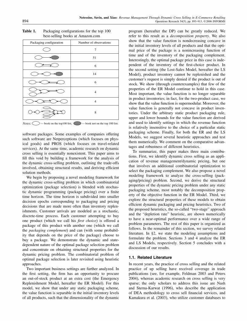
Table 1. Packaging configurations for the top 100best-selling books at Amazon.com
8
4
4
6
14
6
51
7
Number of observationsPackaging configuration
— book on the top100 list,Notes. — book not on the top 100 list.
software packages. Some examples of companies offeringsuch software are Netperceptions (which focuses on phys-ical goods) and PROS (which focuses on travel-relatedservices). At the same time, academic research on dynamiccross selling is essentially nonexistent. This paper aims tofill this void by building a framework for the analysis ofthe dynamic cross-selling problem, outlining the trade-offsinvolved, obtaining structural results, and deriving efficientsolution methods.We begin by proposing a novel modeling framework for
the dynamic cross-selling problem in which combinatorialoptimization (package selection) is blended with stochas-tic dynamic programming (package pricing) over a finitetime horizon. The time horizon is subdivided into smallerdecision epochs corresponding to packaging and pricingdecisions that are made more often than inventory replen-ishments. Customer arrivals are modeled as a stochastic,discrete-time process. Each customer attempting to buyone product (which we call his first choice) is offered apackage of this product with another one (which we callthe packaging complement) and can (with some probabil-ity that depends on the price of the package) choose tobuy a package. We demonstrate the dynamic and state-dependent nature of the optimal package selection problemand concentrate on obtaining structural properties for thedynamic pricing problem. The combinatorial problem ofoptimal package selection is later revisited using heuristicapproaches.Two important business settings are further analyzed. In
the first setting, the firm has an opportunity to procurean out-of-stock product at an extra cost (the EmergencyReplenishment Model, hereafter the ER Model). For thismodel, we show that under any static packaging scheme,the value function is separable in the initial inventory levelsof all products, such that the dimensionality of the dynamic
program (hereafter the DP) can be greatly reduced. Werefer to this result as a decomposition property. We alsoshow that the value function is nondecreasing concave inthe initial inventory levels of all products and that the opti-mal price of the package is a nonincreasing function oftime and of the inventory of the packaging complement.Interestingly, the optimal package price in this case is inde-pendent of the inventory of the first-choice product. Inthe second setting (the Lost-Sales Model, hereafter the LSModel), product inventory cannot be replenished and thecustomer’s request is simply denied if the product is out ofstock. We show (through counterexamples) that few of theproperties of the ER Model continue to hold in this case.Most important, the value function is no longer separablein product inventories; in fact, for the two-product case, weshow that the value function is supermodular. Moreover, thevalue function is generally not concave in product inven-tories. Under the arbitrary static product packaging rule,upper and lower bounds for the value function are derivedand used to identify settings in which the revenue functionis relatively insensitive to the choice of a particular staticpackaging scheme. Finally, for both the ER and the LSModels, we suggest several heuristic approaches and testthem numerically. We comment on the comparative advan-tages and robustness of different heuristics.To summarize, this paper makes three main contribu-
tions. First, we identify dynamic cross selling as an appli-cation of revenue management/dynamic pricing, but onethat involves an additional combinatorial optimization toselect the packaging complement. We also propose a novelmodeling framework to analyze the cross-selling (pack-aging/pricing) problem. Second, we derive the structuralproperties of the dynamic pricing problem under any staticpackaging scheme, most notably the decomposition prop-erty of the objective function in the ER Model. Third, weexplore the structural properties of these models to obtainefficient dynamic packaging and pricing heuristics. Two ofthe proposed heuristics, the so-called “two-stage” approachand the “depletion rate” heuristic, are shown numericallyto have a near-optimal performance over a wide range ofproblem parameters. The rest of this paper is organized asfollows. In the remainder of this section, we survey relatedliterature. In §2, we state the modeling assumptions andformulate the problem. Sections 3 and 4 analyze the ERand LS Models, respectively. Section 5 concludes with adiscussion of our results.
1.1. Related Literature
In recent years, the practice of cross selling and the relatedpractice of up selling have received coverage in tradepublications (see, for example, Feldman 2003 and Peters2004), whereas academic research on cross selling is verysparse; the only scholars to address this issue are Nashand Sterna-Karwat (1996), who describe the applicationof DEA methodology to cross sell financial services, andKamakura et al. (2003), who utilize customer databases to

Netessine, Savin, and Xiao: Revenue Management Through Dynamic Cross Selling in E-Commerce RetailingOperations Research 54(5), pp. 893–913, © 2006 INFORMS 895
identify opportunities for cross selling. To the best of ourknowledge, there are no papers that either model or analyzedynamic cross selling that involves the dynamic pricing ofpackages and dynamic package selection.The seller’s decision to use dynamic package pricing
is closely related to the large stream of operations liter-ature on dynamic pricing and revenue management (seeMcGill and van Ryzin 1999, Bitran and Caldentey 2003,and Talluri and van Ryzin 2004 for extensive surveys). Inanother recent survey, Elmaghraby and Keskinocak (2003)provide a thorough discussion of the need to incorporatecustomized pricing considerations (of which cross selling isone example) into dynamic pricing models; they cite manyapplications and note that there are no papers in the extantliterature addressing this problem. Other publications inthis stream typically consider the dynamic pricing of a sin-gle product, and hence do not address cross-selling issues(see, for example, Gallego and van Ryzin 1994 and Avivand Pazgal 2005). Monahan et al. (2004) study the problemof pricing a single product over multiple time periods aftera single inventory decision. Their setting is similar to oursin that the product is sold over multiple periods without fur-ther replenishments. However, they utilize a specific formof demand function: Random shock is multiplicative andprice dependence is iso-elastic, which allows them to findoptimal prices and inventory in a closed form. An alterna-tive setting is the one in which demand from several typesof customers can be satisfied with the same capacity (seeMaglaras and Meissner 2003). In this paper, demand froma customer may have to be satisfied by several types ofinventory simultaneously. In this respect, we believe thatthe papers most relevant to our work are those analyzingthe dynamic revenue management of multiple products, arather sparsely populated area of literature (see Gallego andvan Ryzin 1997 and Zhang and Cooper 2005).On the Internet, the selection of the packaging com-
plement can be based both on the customer informationacquired during previous transactions and/or on the cus-tomer profile. To process the significant amounts of datanecessary for making decisions, companies utilize data-mining techniques (see Padmanabhan and Tuzhilin 2003for a survey of relevant methodologies). This approach isgenerally termed “personalization” (see Adomavicius andTuzhilin 2002). Papers dealing with personalization tech-niques typically focus on generating a recommendation thatensures the best match between the customer and the prod-uct regardless of the potential impact on the firm’s prof-itability. On the contrary, we assume that the company usesdata mining to generate the probability distribution overcustomers’ purchase preferences, which in turn is used tocross sell products to maximize the firm’s profit. Hence, itis quite possible that the package offered to the customeris not the best possible match from the personalizationperspective.
A practice related to cross selling is product bundling,which also attempts to sell a package of several prod-ucts rather than a single product. However, bundling deci-sions (involving what to bundle and how to price bundles)are static and are made before a customer’s arrival, incontrast to cross selling, which is done only after a cus-tomer declares a desire to buy something. Nevertheless,because dynamic cross selling can be loosely interpretedas dynamic bundling, we shall briefly review the relatedliterature. Economists were the first to analyze the con-cept of bundling (see Stigler 1963). The cornerstone formany subsequent papers on product bundling was the sem-inal work of Adams and Yellen (1976), who formulated amodel with a firm selling two products, as well as a bundleof these two products, and demonstrated the benefits aris-ing from bundling. In the operations literature, Hanson andMartin (1990) were perhaps the first to address the prob-lem of optimally pricing bundles of products using a math-ematical programming approach in a static model. Ernstand Kouvelis (1999) study the issue of how much of eachindividual product, as well as how many bundles, to stockwhen pricing and bundling decisions are exogenous to themodel. A wealth of marketing literature considers bundlingwith particular emphasis on static pricing. Rao (1993) andStremersch and Tellis (2002) review this stream of litera-ture. In addition, an extensive collection of papers on thistopic can be found in Fuerderer et al. (1999). In all ofthese papers, a commitment to sell bundles is made prior tothe arrival of demand, and thereafter prices/bundles cannotbe altered. Hence, the underlying models are static ratherthan dynamic. We are not aware of any papers that analyzedynamic product bundling.
2. Modeling Dynamic Cross-SellingDecisions
We consider an environment in which an online retail com-pany sells a group of m products. We assume that all prod-ucts in the group target similar market segments or arecomplementary and can therefore potentially be cross soldwith each other (see the examples in the introduction). Wefurther assume that the planning horizon is finite (represent-ing the time between two inventory replenishments) and isseparated into N decision epochs. At the beginning of eachdecision epoch, the company observes the inventory of eachproduct and makes cross-selling (packaging and pricing)decisions. In the online environment, packaging and pricingdecisions can be made as frequently as necessary, so thatthe length of each decision epoch can be made short com-pared to typical customer interarrival time. Consequently,we assume that within each epoch, there is at most one cus-tomer arrival.3 We denote by �i� i= 1� � � � �m, the probabil-ity that during any decision epoch class i customer arrivesand requests one unit of the ith product (
∑mi=1 �i < 1 to
reflect the possibility that there is no customer arrival ina particular decision epoch). Alternatively, one can also
Netessine, Savin, and Xiao: Revenue Management Through Dynamic Cross Selling in E-Commerce Retailing896 Operations Research 54(5), pp. 893–913, © 2006 INFORMS
define the probability that arriving customers do not buya product, but the problem can easily be reformulated tofocus on customers who are willing to make a purchase.4
Upon requesting product i at a fixed price5 pi, a class icustomer receives an offer of a “product i-product j” pack-age (for some j) at a price pij . We assume that onlyone package of only two products is offered to the cus-tomer, which is consistent with the practice of some com-panies. For example, our experiment with Amazon.com’sbest-seller list (see Table 1) shows that at most one packag-ing complement is offered for each available product. Weassume that class i customers have a reservation price forthe ij package distributed according to a cumulative dis-tribution function Fij�·� with nonnegative support. Conse-quently, a class i customer buys the package at a price pijwith probability �Fij�pij �= 1−Fij�pij �, and buys only prod-uct i at price pi with probability Fij�pij �.
6 We assume that�Fij�x��x− y� is a unimodal function of x for any nonneg-ative constant y. This assumption holds for a wide classof distribution functions and is also a standard assumptionoften made in the pricing literature (see Ziya et al. 2004for a discussion and references). While it may seem natu-ral to restrict the support of the reservation price functionFij�pij � to pi � pij � pi + pj , we do not make this explicitassumption because it is not inconceivable that a companywould attach a value to the very offer of a packaging com-plement, which potentially saves the customer some searchtime (in fact, in the authors’ experience, major Web-basedtravel agents may sometimes sell travel packages at a pre-mium). This is possible because the customer observes onlythe individual price of product i, but may not be aware ofthe individual price for product j . Note that the reserva-tion price function Fij�pij � can always be defined so thatFij�pij �= 1 for pij = pi+pj .The issue of estimating Fij�pij � is an important one
that merits a separate study. For our purposes, we sim-ply assume that Fij�pij � is obtained by analyzing cus-tomer shopping behavior using data-mining techniques.Two examples of approaches that can potentially be used inthis case are found in Moe and Fader (2004) and Bertsimaset al. (2003). Because we do not assume any particularfunctional form for these probability functions, our modelcan accommodate any approach. Note also that we classifycustomers based on the product they request, while in prac-tice a company may have additional customer informationthat would allow for fine tuning the probability estimationfurther. In the extreme, each arriving customer could betreated as a separate class. Our model can be extended toallow for such a possibility (e.g., let k be the customerindex with each customer having a unique k so that �i =∑k �
ki , where �
ki represents customer k arriving to request
book i), but at a cost of additional notation that would makeexposition less tractable. Supporting our approach is someevidence that for a cross-selling recommendation, the first-choice product is more relevant than the customer profile(see Weigend 2004).
In each decision epoch a company needs to decide, foreach product i, which product j should be packaged withit and what price should be established for such a pack-age. Suppose that at the beginning of the nth decisionepoch �n= 1� � � � �N � the inventory levels of products aregiven by vector I= �I1� � � � � Im�, and let Vn�I� be the opti-mal expected revenue accrued from that moment until theend of the planning horizon. Define ei, i = 1� � � � �m, asan m-dimensional vector whose components are �ei�k = 1if k = i and 0 otherwise. We are interested in selectinga sequence of packaging and pricing decisions to maxi-mize V1�I�. The functional form of the Bellman equationfor Vn�I� depends on actual inventory levels. If there isat least one unit of inventory for each product �Ii � 1 forall i= 1� � � � �m; the situation with Ii = 0 will be consideredshortly), the Bellman equation can be expressed as
Vn�I�=m∑i=1�imax
j �=i
(maxpij
(Fij�pij ��pi+Vn+1�I−ei��
+ �Fij�pij ��pij+Vn+1�I−ei−ej ��))
+(1−
m∑i=1�i
)Vn+1�I�� (1)
At the heart of recursion (1) are two maximizationoperators reflecting the dynamic packaging and pricingdecisions. The “outer” maximization selects the “best”product j to be packaged with product i in the case ofa class i customer arrival, while the “inner” maximizationselects the “best” price for each ij package. Without loss ofgenerality, we assume that the inventory left in stock at theend of the planning horizon has no salvage value and sup-plement (1) by the “end-of-horizon” condition VN+1�I�= 0.Clearly, the dynamic packaging problem is quite com-
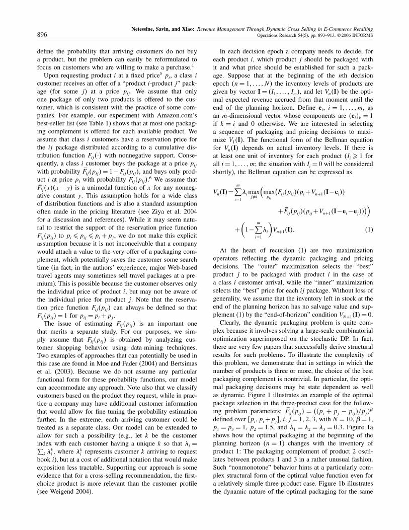
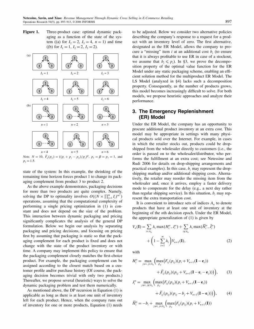
plex because it involves solving a large-scale combinatorialoptimization superimposed on the stochastic DP. In fact,there are very few papers that successfully derive structuralresults for such problems. To illustrate the complexity ofthis problem, we demonstrate that in settings in which thenumber of products is three or more, the choice of the bestpackaging complement is nontrivial. In particular, the opti-mal packaging decisions may be state dependent as wellas dynamic. Figure 1 illustrates an example of the optimalpackage selection in the three-product case for the follow-ing problem parameters: �Fij�pij � = ��pi + pj − pij�/pj��defined over �pi� pi+pj�, i� j = 1�2�3, with N = 10, �= 1,p1 = p3 = 1, p2 = 1�5, and �1 = �2 = �3 = 0�3. Figure 1ashows how the optimal packaging at the beginning of theplanning horizon �n = 1� changes with the inventory ofproduct 1: The packaging complement of product 2 oscil-lates between products 1 and 3 in a rather unusual fashion.Such “nonmonotone” behavior hints at a particularly com-plex structural form of the optimal value function even fora relatively simple three-product case. Figure 1b illustratesthe dynamic nature of the optimal packaging for the same
Netessine, Savin, and Xiao: Revenue Management Through Dynamic Cross Selling in E-Commerce RetailingOperations Research 54(5), pp. 893–913, © 2006 INFORMS 897
Figure 1. Three-product case: optimal dynamic pack-aging as a function of the state of the sys-tem ((a) for I2 = 2, I3 = 4, n = 1) and time((b) for I1 = 1, I2 = 2, I3 = 2).
I1 = 1 I1 = 2 I1 = 3
I1 = 4 I1 = 5 I1 = 6
1
2
3
1
2
3
1
2
3
1
2
3
1
2
3
1
2
3
n = 1 n = 2 n = 3
n = 4 n = 5 n = 6
1
2
3 1
2
3 1
2
3
1
2
3 1
2
3 1
2
3
(a)
(b)
Note. N = 10, �Fij �pij � = ��pi + pj − pij �/pj��, p1 = � = p3 = 1, andp2 = 1�5�
state of the system: In this example, the shrinking of theremaining time horizon forces product 1 to change its pack-aging complement from product 3 to product 2.As the above example demonstrates, packaging decisions
for more than two products are quite complex. Namely,solving the DP to optimality involves O��N ×∏m
i=1 Ii�m2�
operations, assuming that the computational complexity ofperforming a single pricing optimization in (1) is con-stant and does not depend on the size of the problem.This interaction between dynamic packaging and pricingsignificantly complicates the analysis of the general DPformulation. Below we begin our analysis by separatingpackaging and pricing decisions, and focusing on pricingfirst by assuming that packaging is static so that the pack-aging complement for each product is fixed and does notchange with the state of the product inventory or withtime. A company may implement this policy to ensure thatthe packaging complement closely matches the first-choiceproduct. For example, the packaging complement can beassigned according to the closest match based on a cus-tomer profile and/or purchase history (Of course, the pack-aging decision becomes trivial with only two products.)Thereafter, we propose several (heuristic) ways to solve thedynamic packaging problem and test them numerically.As mentioned above, the DP recursion in Equation (1) is
applicable as long as there is at least one unit of inventoryleft for each product. Hence, when the company runs outof inventory for one or more products, Equation (1) needs
to be adjusted. Below we consider two alternative policiesdescribing the company’s response to a request for a prod-uct with an inventory level of zero. The first alternative,designated as the ER Model, allows the company to pro-cure a “missing” item i at an additional cost bi (to ensurethat it is always profitable to use ER in case of a stockout,we assume that bi � pi). In §3, we prove the decompo-sition property of the optimal value function for the ERModel under any static packaging scheme, enabling an effi-cient solution method for the multiproduct ER Model. TheLS Model (analyzed in §4) lacks such a decompositionproperty. Consequently, as the number of products grows,this model becomes increasingly difficult to solve. For bothmodels, we propose heuristic approaches and analyze theirperformance.
3. The Emergency Replenishment(ER) Model
Under the ER Model, the company has an opportunity toprocure additional product inventory at an extra cost. Thismodel may be appropriate in settings with many physi-cal products sold over the Internet. For example, in casesin which the retailer stocks out, products could be drop-shipped from the wholesaler directly to customers (i.e., theorder is passed on to the wholesaler/distributor, who per-forms the fulfillment at an extra cost; see Netessine andRudi 2006 for details on drop-shipping arrangements andpractical examples). In this case, bi may represent the drop-shipping markup and/or additional shipping costs. Alterna-tively, the retailer may reorder the missing item from thewholesaler and, once it arrives, employ a faster deliverymode to compensate for the delay (e.g., a next day ratherthan regular shipping service). In this situation, bi may rep-resent the extra transportation cost.It is convenient to introduce sets of indices An to denote
products that have at least one unit of inventory at thebeginning of the nth decision epoch. Under the ER Model,the appropriate generalization of (1) is given by
Vn�I�=∑i∈An�imax�H
ni � J
ni �+
∑iAn�imax� �Hn
i � Jni �
+(1−
m∑i=1�i
)Vn+1�I�� (2)
with
Hni = max
j �=i� j∈An
(maxpij
(Fij�pij ��pi+Vn+1�I− ei��
+ �Fij�pij ��pij +Vn+1�I− ei− ej ��))� (3)
J ni = maxj �=i� jAn
(maxpij
(Fij�pij ��pi+Vn+1�I− ei��
+ �Fij�pij ��pij − bj +Vn+1�I− ei��))� (4)
�Hni =−bi+ max
j �=i� j∈An
(maxpij
(Fij�pij ��pi+Vn+1�I��

Netessine, Savin, and Xiao: Revenue Management Through Dynamic Cross Selling in E-Commerce Retailing898 Operations Research 54(5), pp. 893–913, © 2006 INFORMS
+ �Fij�pij ��pij +Vn+1�I− ej ��))� (5)
J ni =−bi+ maxj �=i� jAn
(maxpij
(Fij�pij ��pi+Vn+1�I��
+ �Fij�pij ��pij − bj +Vn+1�I��))� (6)
Note that in this case all product indices remain “active”due to the possibility of outsourcing the “missing” product.Equations (3)–(6) reflect four distinct packaging possibili-ties that potentially exist under the ER Model. For example,if an in-stock product is requested, it can be matched withanother in-stock product (3), or with an out-of-stock prod-uct (4), with corresponding penalty. Similarly, if an out-of-stock product is requested, it will be procured at an extracost, and it can be packaged with an in-stock product (5),or with another out-of-stock product (6).
3.1. Dynamic Pricing Under Static Packaging
Let j�i� be the index of the product offered in a packagewith product i when a class i customer arrives. Under thestatic packaging utilized in this section, j�i� is fixed foreach i = 1�2� � � � �m. We denote by E�i� the set of prod-ucts for each of which product i is offered as a packagingcomplement, E�i�= �k � j�k�= i�. For the ER Model withstatic packaging, (2) can be simplified to
Vn�I�=m∑i=1�imax
pi� j�i�Y ni� j�i�+
(1−
m∑i=1�i
)Vn+1�I�� (7)
with
Y nij =
Fij�pij ��pi+Vn+1�I−ei��+ �Fij�pij �·�pij+Vn+1�I−ei−ej �� if i∈An�j ∈An�
Fij�pij ��pi+Vn+1�I−ei��+ �Fij�pij �·�pij−bj+Vn+1�I−ei�� if i∈An�jAn�
−bi+Fij�pij ��pi+Vn+1�I��+ �Fij�pij �·�pij+Vn+1�I−ej �� if iAn�j ∈An�
−bi+Fij�pij ��pi+Vn+1�I��+ �Fij�pij �·�pij−bj+Vn+1�I�� if iAn�jAn�
(8)
It turns out that under the assumption of static packagingin the ER Model, the m-dimensional DP (7) can be decom-posed into m one-dimensional DPs. Such decompositiongreatly reduces the computational effort necessary for solv-ing (7). Below we present the decomposition property ofthe ER Model under static packaging. We start by intro-ducing the following definition:
Definition 1. For i= 1� � � � �m, let Gin�Ii� be the functionsatisfying the following recursive formulae:
Gin�Ii�= �i�pi+Gin+1�Ii−1��+(1−�i−
∑j∈E�i�
�j
)Gin+1�Ii�
+ ∑j∈E�i�
�j maxpji
(Fji�pji�G
in+1�Ii�
+ �Fji�pji��pji−pj +Gin+1�Ii− 1��)
(9)
for Ii � 1 and n= 1� � � � �N , and
Gin�0�= �i�pi+Gin+1�0�−bi�+(1−�i−
∑j∈E�i�
�j
)Gin+1�0�
+ ∑j∈E�i�
�j maxpji
(Fji�pji�G
in+1�0�
+ �Fji�pji��pji−pj +Gin+1�0�− bi�)� (10)
while GiN+1�Ii�= 0.
Note that (10) can be expressed in closed form as fol-lows:
Gin�0�= �N + 1− n�(�i�pi− bi�
+ ∑j∈E�i�
�j maxpji� �Fji�pji��pji−pj − bi��
)� (11)
The following result states the decomposition propertyof the optimal revenue function:
Proposition 1. In each decision epoch n, the optimal ex-pected revenue function described by (7) can be separatedinto m parts, with each depending only on the inventorylevel of a single product:
Vn�I�=m∑i=1Gin�Ii�� n= 1� � � � �N + 1�
where Gin�Ii� is defined by (9)–(10).
Proof. See the appendix.
We note that Gin�Ii� can be interpreted as the expectedrevenue generated by the inventory of product i alone.Indeed, as (9) suggests, product i’s inventory can bechanged either directly through sales to class i customersor indirectly through sales to class j �= i customers as partof a ji package. In the first case, the revenue generated perunit of product i sold is pi, while in the second case it ispji−pj .The decomposition result is somewhat surprising: One
might expect that the opportunity to procure missing itemswould complicate, not simplify, the problem (a similarobservation is made in Plambeck and Ward 2003). We notethat the result of Proposition 1 can be rationalized as fol-lows: It can be shown that under static packaging, the valuefunction of the “main” dynamic program (1) is decompos-able into the sum of single-product functions. The sameis true for the “boundary” conditions in (7) relating to theterms in (8) with i or j outside of An, and the decomposi-tion “pieces” (single-product value functions) are identicalin both cases. As it turns out, such matching of decompo-sition pieces does not hold for the LS Model, nor does thedecomposition result of Proposition 1. At the same time,as we will show later, the decomposition of (1) can still be
Netessine, Savin, and Xiao: Revenue Management Through Dynamic Cross Selling in E-Commerce RetailingOperations Research 54(5), pp. 893–913, © 2006 INFORMS 899
applied heuristically in the LS case to yield good perfor-mance and thus has applicability beyond the ER Model.Next, we use the decomposition property of the rev-
enue function to derive additional structural properties. Wedenote by p∗ij �I� n� the optimal package price in decisionepoch n given that the inventory levels of products are I.
Proposition 2. (a) Gin�Ii� is a nondecreasing concavefunction of Ii for i= 1� � � � �m, and n= 1� � � � �N .(b) The optimal package price p∗ij �I� n� is nonincreas-
ing in n, Ij , and is independent of Ik for k �= j , for i� j =1� � � � �m and i �= j .Proof. See the technical online appendix at http://or.pubs.informs.org/Pages.collect.html.
The results of Proposition 2 are established using theinduction over the time index n. We note that concav-ity of the revenue functions Gin�Ii� facilitates the connec-tion between the cross-selling problem we consider and theinventory-ordering problem the online retailer may face.In particular, concave revenue functions can be included,along with convex inventory holding costs, in the general-ized inventory-ordering problem. Thus, in the absence ofjoint inventory-ordering costs, the optimal inventory pol-icy for each item remains an �s� S� policy (see Scarf 1960,Veinott 1966, and Zheng 1991). For situations in whichjoint ordering costs are significant, the �s� S� policy is nolonger optimal. For such cases, however, Zheng (1994)proves that a modified �s� S� policy, a so-called �s� c� S�policy, is optimal in the decentralized system. Federgruenet al. (1984) provide an iterative procedure to repeatedlyupdate the �s� c� S� values for each item until the optimumis reached.The second part of Proposition 2 indicates that the opti-
mal package price is nondecreasing in “time-to-go” andnonincreasing in the inventory of the packaged product.The first effect is similar to the one found in single-product dynamic pricing problems (see Gallego and vanRyzin 1994). The second effect is quite intuitive and showsthe linkage between product availability and price that wehypothesized in the introduction. These findings are insome ways unsurprising because they also hold in simplersettings when a seller dynamically prices a single prod-uct. Nevertheless, it is reassuring that under a detailed andexplicit model of cross selling, this property still holds.Finally, the inventory of the first-choice product does notaffect package price due to the decomposition property ofthe value function.
3.2. Heuristic Approaches to DynamicPackaging and Pricing
The optimal solution to the cross-selling problem (1)may be hard to obtain in real time in cases involving alarge number of products. Even though the decompositionproperty can be applied to simplify the pricing problem,the combinatorial optimization aimed at finding the best
packaging complements still poses a significant challenge.In this section, we propose and test numerically severalheuristic packaging-pricing approaches. First, we presentthe myopic heuristic HM , which ignores product inventoriesand time-to-go. To account for these factors, we con-sider two more sophisticated heuristic approaches. Heuris-tic HD characterizes the optimal solution in the ER Modelwith one-shot static and deterministic demand whose valuedepends on packaging and pricing decisions. This solu-tion can then be used dynamically at each point in timein response to changing inventory levels. The heuristic HT
simplifies the solution to the DP by assuming that there areno packaging decisions in any periods other than the cur-rent one. Finally, the heuristic HDR makes decisions basedon the easily computable index.
3.2.1. Myopic Packaging and Pricing Heuristic. Per-haps the simplest approach to pricing and packaging isto ignore the impact of product inventories. We denotethe resulting myopic static packaging and pricing heuristicas HM . From (9), assuming that Gin+1�Ii� = Gin+1�Ii − 1�,we obtain
jM�i�= argmaxj �=i
�Fij�pMij ��pMij −pi�� i= 1� � � � �m� (12)
where pMij is defined by
pMij = argmaxpij
� �Fij�pij ��pij −pi��� (13)
The static packaging scheme defined by (12) myopi-cally chooses the packaging complement to maximize theexpected profit from selling a package. Note that (12)serves as the fundamental characteristic of class i cus-tomers’ propensity to buy product j and represents the opti-mal price to be charged for the ij package in the caseof infinite product j inventory. The clear advantage of themyopic approach is its implementational and computationalsimplicity: Its application requires only O�m2� comparisons(here and below we assume that the time required to per-form an optimization of type (13) is constant and does notdepend on the problem size). On the other hand, the myopicheuristic assumes that the marginal value of the inventoryof the potential packaging complement is negligible—anassumption that can be especially inadequate in cases inwhich product inventories are constrained.
3.2.2. Static Deterministic Approximation. Considera static deterministic approximation to the dynamic andstochastic ER Model. We assume that the “one-shot”demand for each package and each single product is deter-ministic, but influenced by packaging and pricing deci-sions. Specifically, we introduce the time parameter ( =N − n, which plays the role of the effective time horizonin our static deterministic analysis. In particular, the totaldemand from type i customers is �i( . Packaging decisionsare defined by the fraction of type i demand, 0 � qij � 1,which receives an offer of the ij package (this is differentfrom the ji package). Note that these continuous variables
Netessine, Savin, and Xiao: Revenue Management Through Dynamic Cross Selling in E-Commerce Retailing900 Operations Research 54(5), pp. 893–913, © 2006 INFORMS
represent a generalization of the packaging decisions intro-duced in §2, which simplifies the analysis of the determin-istic model we consider. Given any packaging decisions�qij� and pricing decisions �pij�, the total demand for theij package is given by �i(qij �Fij�pij �, and the total demandfor a single product i is given by
∑j �=i �i(qijFij �pij � for
i� j = 1�2� � � � �m and i �= j .Our static deterministic approximation assumes that the
demand for each package and each single product isthe expected value of the corresponding demand arising inthe stochastic setting, given that the same static packagingand pricing decisions are used. The objective is to maxi-mize the total revenue minus the total emergency replenish-ment cost by selecting the optimal values of �qij� and �pij�.This static problem, denoted as (P1), can be formulated asfollows:
�P1� maxqij � pij
m∑i=1
∑j �=i�i(qij �Fij�pij �pij +
m∑i=1
∑j �=i�i(qijFij �pij �pi
−m∑i=1bi
(�i( +
∑j �=i�j(qji �Fji�pji�− Ii
)+
s.t.∑j �=iqij = 1 for i= 1�2� � � � �m�
qij � 0 for i �= j�where x+ =max�x�0�. The first part in this objective func-tion represents the total revenue collected from selling allij packages, the second part is the total revenue from sell-ing individual products, and the third part is the purchasecost for ERs derived from the fact that the total demand forproduct i consists of demand
∑j �=i �i(qijFij �pij � for indi-
vidual product i, demand∑j �=i �i(qij �Fij�pij � for all ij pack-
ages, and demand∑j �=i �j(qji �Fji�pji� for all ji packages.
Note that (P1) belongs to the class of constrained opti-mization problems with nondifferentiable objective func-tions, which, in general, are hard to cope with. Next, weconsider a modified problem (P2) that is equivalent to (P1),but is easier to solve. We then formulate the dual prob-lem (D2) of the primal problem (P2) and show that theoptimal solution to (P2) can be derived easily from theoptimal solution to (D2), whose objective function is linearand whose constraint set is convex. Thus, many existingalgorithms (e.g., the gradient method) can be applied tosolve (D2), which is equivalent to solving (P1).By introducing auxiliary variables �yi� and performing
some algebraic manipulations on the objective function,problem (P1) can be formulated as the following equivalentproblem (with the objective value differing by a constant),denoted by (P2):
�P2� maxyi� qij � pij
m∑i=1
∑j �=i�j(qji �Fji�pji��pji−pj�−
m∑i=1biyi
s.t. yi � �i( +∑j �=i�j(qji �Fji�pji�− Ii
for i= 1�2� � � � �m�
∑j �=iqij = 1 for i= 1�2� � � � �m�
yi � 0 for i= 1�2� � � � �m�
qij � 0 for i �= j�
Define Hji�x� = maxpji ��Fji�pji��pji − pj − x��. The main
results of this subsection are summarized in the followingproposition.
Proposition 3. (a) The dual problem (D2) of the primalproblem (P2) can be formulated as the following optimiza-tion problem with a convex set of constraints:
�D2� min*i� vi
m∑i=1�*i�Ii−�i(�+ vi�
s.t. �j(Hji�*i�� vj for i �= j�0�*i � bi for i= 1�2� � � � �m�
(b) Given any optimal solution �*∗i � v
∗i � to (D2), there
exists a corresponding optimal solution ��p∗ij �� �q∗ij �� �y
∗i ��
to (P2), determined as follows:(i) p∗ji = argmaxpji �
�Fji�pji��pji−pj −*∗i �� for i �= j;
(ii) �q∗ij � and �y∗i � are the solutions to (P2), with pij
replaced by p∗ij .
Proof. See the appendix.
Proposition 3b(i) indicates that the dual solution *∗i can
be interpreted as the marginal value of an extra unit ofproduct i. That is, if there is ample inventory, there is noneed to make an emergency replenishment of product i,and thus *∗
i = 0. On the other hand, if the inventory isscarce, then *∗
i is equal to the ER cost bi. In other words,*∗i can also serve as an availability indicator for prod-
uct i. By the equivalence of (P1) and (P2), the optimalsolution �p∗ij � q
∗ij � derived from Proposition 3b is also opti-
mal for (P1). This optimal solution yields another dynamiccross-selling heuristic in which decisions depend on thecurrent product inventory and time-to-go. In the dynamicstochastic environment of (1), this heuristic (which wedenote as HD) is implemented as follows: At the beginningof each decision epoch n, (P2) is solved for ( = N − nusing current product inventory levels. The obtained pack-aging ��q∗ij �� and pricing ��p∗ij �� solutions are used as fol-lows: When a customer of class i arrives, a firm conductsa randomized “coin-flip” trial (with the probability of thejth outcome being q∗ij ); the realized outcome j is selectedand the ij package is offered at the price p∗ij . In terms ofcomputational complexity, this heuristic involves solvingO�N� convex optimizations (D2) and linear programmingproblems (P2) (where the optimal values of Pij are pre-determined by Proposition 3(b)(i)).

Netessine, Savin, and Xiao: Revenue Management Through Dynamic Cross Selling in E-Commerce RetailingOperations Research 54(5), pp. 893–913, © 2006 INFORMS 901
3.2.3. A Two-Stage Heuristic. Suppose that at thebeginning of the nth decision epoch the current inventoryvector is I. Under the “two-stage” approach, we simplifythe packaging/pricing problem by assuming that there is nopackaging in periods n+ 1 through N . Note that the num-ber of type i customers arriving in each epoch is a Bernoullirandom variable with parameter �i and the number of type icustomers arriving in all remaining N −n epochs is a bino-mial random variable -i with parameters ��i�N −n�. Then,the marginal value of an extra unit of product j �= i can beexpressed as
Vn+1�I− ei�−Vn+1�I− ei− ej �
= bjE�min�-j� Ij�−min�-j� Ij − 1��
= bj Pr�-j � Ij�= bjN−n∑k=Ij
(N − nk
)�kj �1−�j�N−n−k� (14)
The package price pTij for any �i� j� combination can beestablished from
.Vn�I�/.pij
= fij �pij ��pi+Vn+1�I− ei��
− fij �pij ��pij +Vn+1�I− ei− ej ��+ �Fij�pij �=−fij �pij �
(pij −pi− �Vn+1�I− ei�−Vn+1�I− ei− ej ��
)+ �Fij�pij �= 0� (15)
so that after substituting (14) into (15) and rearranging, weobtain7
pTij = pi+ �Fij�pTij �/fij �pTij �
+ bjN−n∑k=Ij
(N − nk
)�kj �1−�j�N−n−k� (16)
Note that the expression for the myopic price pMij intro-duced earlier does not contain the last term appearingin (16): pTij (in which T stands for the heuristically calcu-lated terminal value of inventory) is an upper bound on pMij .At the same time, pTij is a lower bound on the optimal pricebecause packaging in subsequent periods is not accountedfor. Also note that the value of pTij explicitly depends onthe inventory of product j .The packaging complement for product i is then deter-
mined as follows. Suppose that customer i arrives andwe decide not to offer any package. Then, we earn pi +Vn+1�I− ei�. The incremental value (denoted by 0ij ) ofoffering the package ij can be calculated as follows:
0ij =(Fij�p
Tij ��pi+Vn+1�I− ei��+ �Fij�pTij �
·�pTij+Vn+1�I−ei−ej ��)−�pi+Vn+1�I−ei��
= �Fij�pTij �(pTij −pi− �Vn+1�I− ei�−Vn+1�I− ei− ej ��
)= �Fij�pTij �
(pTij −pi− bj
N−n∑k=Ij
(N − nk
)�kj �1−�j�N−n−k
)
= � �Fij�pTij ��2/fij �pTij � (from (16))�
Hence, we propose the following dynamic packaging/pric-ing heuristic HT : When a customer of type i arrives, wecalculate pTij for all j using (16). Then, the values of 0ijare computed for all j , and the index of the highest valueis selected:
jT �i�= argmaxj �=i
�� �Fij�pTij ��2/fij �pTij ��� (17)
We observe that under the two-stage heuristic, both thepackaging and the pricing decisions are truly dynamic:Both depend on current product inventories as well as ontime-to-go. Assuming, as before, that the time it takes toperform an optimization of type (13) is constant and doesnot depend on problem size, we establish that the compu-tational complexity of this heuristic is O�Nm2�.To illustrate packaging decisions under HT , we consider
an example with the exponential price reservation function� �Fij�pij �= exp�−�ij�pij−pi���, symmetric price-sensitivityfactors �ij , which depend only on the index of the first-choice product rather than on the index of the packag-ing complement ��ij = �i�, and symmetric penalty costs�bj = b�. In this case, we obtain
pTij = pi+1�i
+ bN−n∑k=Ij
(N − nk
)�kj �1−�j�N−n−k
and, after some algebra,
jT �i�= argmaxj �=i
( Ij∑k=0
(N − nk
)�kj �1−�j�N−n−k
)�
Note that the expression
S�n� Ij � �j�=Ij∑k=0
(N − nk
)�kj �1−�j�N−n−k
is an increasing function of the inventory Ij , and the deci-sion epoch n is a decreasing function of demand inten-sity �j and does not depend on the index of the first-choiceproduct i. In other words, S�n� Ij � �j� can be interpretedas a proxy of how well product j has been selling up tothe decision epoch n: the lower the value of this expres-sion, the closer the product to the status of best-seller.Thus, the price of the ij package (when it is offered) is,as expected, a decreasing function of Ij and of the deci-sion epoch n and an increasing function of the demandintensity �j . The set of packaging complements can beestablished as follows: At each decision epoch n, rank allproducts according to the current value of the parameterS�n� Ij � �j� and let j Ts = argmaxj �S�n� Ij � �j�� and j
Tn =
argmaxj �=jTs �S�n� Ij � �j�� be the indices of products withthe highest and second-highest parameter values (note thatif more than one product currently has the same parametervalue, ties can be broken arbitrarily). Then, (17) is equiva-lent to
jT �i�=j Ts � i �= j Ts �jTn � i= j Ts �
(18)
Netessine, Savin, and Xiao: Revenue Management Through Dynamic Cross Selling in E-Commerce Retailing902 Operations Research 54(5), pp. 893–913, © 2006 INFORMS
In view of our interpretation of S�n� Ij � �j� as the best-selling index, the packaging in (18) is intuitively appealing:All products are offered in a package with the current slow-est seller, and the slowest seller itself is packaged with thecurrent second-slowest seller.
3.2.4. The Depletion Ratio Heuristic. Our discussionof the two-stage heuristic indicates that dynamic crossselling can be viewed as an effective tool for redirect-ing the demand for best-selling products to products withslower-than-desired sales. Below we propose another easy-to-implement dynamic packaging approach that we call the“depletion ratio” (DR) heuristic, which emphasizes the roleof dynamic packaging in the cross-selling process. Underthe DR heuristic �HDR�, in each decision epoch n, eachproduct i is assigned a “depletion ratio” index equal to theratio of the current product inventory Ii to the rate �i atwhich product inventory would be depleted in the absenceof cross selling. Defined in this way, the DR index plays arole similar to S�n� Ij � �j� defined for the two-stage heuris-tic under the exponential reservation price function: It indi-cates the current sales ranking of each product. For thecurrent set of inventory values, let js = argmaxi�Ii/�i� andjn = argmaxi �=js �Ii/�i� be the indices of the slowest-sellingand the second slowest-selling products, respectively. Then,the dynamic packaging decisions under the DR approachcan be described as follows:
jDR�i�={js� i �= js�jn� i= js�
(19)
The intuition behind the choice of the cross-selling comple-ment in (19) is similar to the intuition behind (18): Everyproduct is packaged with the current slowest seller, whilethe slowest seller itself is packaged with the current second-slowest-selling product. Note that the DR approach doesnot restrict the choice of the package-pricing policy andcan be combined with simple static pricing or sophisti-cated optimal dynamic pricing. In particular, in our anal-ysis below we consider two cross-selling policies basedon DR packaging. The first policy, which we call the“myopic” DR policy �HDRM�, complements DR packag-ing with the myopic pricing defined by (13). More specif-ically, under the DRM heuristic, in the decision epoch nproduct i is offered in a bundle with product jDR�i�, andthe price requested for such a bundle is equal to pDRMi =argmaxp� �FijDR�i��p��p− pi��. The second DR-based cross-selling policy �HDRO� selects the best pricing under DRpackaging by solving the variant of (1) with packagingcomplements determined by (19). More specifically, theDRO heuristic combines DR bundling with the pricingdetermined by solving the following dynamic program:
Vn�I�=m∑i=1�imax
p
(FijDR�i��p��pi+Vn+1�I− ei��
+ �FijDR�i��p��p+Vn+1�I− ei− ej ��)
+(1−
m∑i=1�i
)Vn+1�I� (20)
with the usual boundary conditions. We note that the com-plexity of computing the heuristic prices and bundlingcomplements for HDRM is O�Nm2�, while the respectivecomputational complexity for the HDRO heuristic is O��N ×∏mi=1 Ii�
m�.Despite the intuitive nature of DR packaging, an analyti-
cal characterization of sufficient conditions for its optimal-ity is hard to obtain, except in rather restrictive settings.Below we provide an example of such conditions understatic pricing in a symmetric product environment.
Proposition 4. Let �i = �, pi = p, bi = b, pij = q, p <q < p + b, and �Fij�pij � = 1 for any j �= i and i� j =1�2� � � � �m. Then, DR packaging is optimal for any deci-sion epoch n= 1� � � � �N .
Proof. See the appendix.
Proposition 4 considers the setting in which productpackages are being sold at a fixed price and the productsdiffer only in their inventory values. While Proposition 4indicates the potential effectiveness of the DR packag-ing approach in nearly symmetric environments with staticpackage pricing, its performance in more typical settingsneeds to be evaluated numerically.
3.2.5. Effectiveness of Packaging and Pricing Heuris-tics: Numerical Study. In this section, we use an ex-tensive numerical study to test the effectiveness of pric-ing/packaging heuristics for the ER Model. We denote byROPT the optimal expected profits obtained by solving (2)(note that computing the optimal dynamic packaging andpricing policy requires solving an m-dimensional DP). Foreach cross-selling heuristic 2, we compute the value of itsexpected profits as follows. In each decision epoch n, letj2�n� i� be the packaging complement that the heuristic 2selects for product i, and also denote by p2�n� i� the pricecharged for the i− j2�n� i� package. Then, for any initialinventory vector, the expected profits under 2 are evaluatedusing the iteration
V 2n �I�=m∑i=1�i(Fij2 �n� i��p
2�n� i���pi+V 2n+1�I− ei��)
+ �Fij2 �n� i��p2�n� i���p2�n� i�+V 2n+1�I− ei− ej ��
+(1−
m∑i=1�i
)V 2n+1�I� (21)
for I > 0, n = 1� � � � �N , with appropriate boundary con-ditions. We probe the effectiveness of the HM , HD, HT ,HDRM , and HDRO heuristics in the ER Model by comparingthe relative performance gaps between RM , RD, RT , RDRM ,RDRO, and ROPT 4 5k = 100%× �ROPT −Rk�/ROPT , k =M�D�T �DRM�DRO.
The Case of m= 3 Products and Exponential Reser-vation Price Functions. Our search at Amazon.comreveals that in most instances the number of products

Netessine, Savin, and Xiao: Revenue Management Through Dynamic Cross Selling in E-Commerce RetailingOperations Research 54(5), pp. 893–913, © 2006 INFORMS 903
connected through packaging is three or less (see Table 1).To reflect this observation in our numerical study, we fixedthe number of products that can be potentially connectedthrough packaging at m = 3. Recall that with three prod-ucts optimal packaging decisions are, generally speaking,state dependent and dynamic.Our test suite was designed as follows. To isolate the
effects of package pricing, we set the prices for individualproducts at the same level: p1 = p2 = p3 = 1. For pack-age reservation prices, we use the “exponential” distribu-tion functions �Fij�pij � = exp�−�ij�pij − pi��, and assumefor simplicity that the price-sensitivity factors �ij dependonly on the index of the first-choice product rather thanon the index of the packaging complement: �i = �ij ∀ i� j .In our numerical study, each of the price-sensitivity factorstakes a value of 1 (“low sensitivity”), 2 (“medium sensi-tivity”), 5 (“high sensitivity”), or 20 (“very high sensitiv-ity”). We set the number of time periods at N = 20 andfix the total customer arrival rate at �= �1 +�2 +�3 = 0�8.The “individual product” arrival rates are varied as fol-lows: �1 = 0�1+ 0�561, �2 = 0�1+ �0�6− �1�62, and �3 =0�8−�1 −�2, where both 61 and 62 take values of 0, 0.5,and 1. Hence, we allow seven possible combinations ofarrival rates: �0�1�0�1�0�6�, �0�1�0�6�0�1�, �0�6�0�1�0�1�,�0�1�0�35�0�35�, �0�35�0�1�0�35�, �0�35�0�35�0�1�, and�0�35�0�225�0�225�. These combinations cover three essen-tial scenarios for a three-way splitting of total demand:“mostly single-product arrivals” (the first three), “mostlytwo-product arrivals” (the next three), and “closely-valueddemands” (the last one).To test the sensitivity of the heuristics with respect to the
initial levels of product inventory, we investigate the casesin which the initial inventories are set at Ii = �1+ 1��iN ,i= 1�2�3, where the “inventory availability” coefficient 1takes values of −0�8 (“severely constrained inventory”),−0�3 (“moderately constrained inventory”), 0 (“inventorymatching demand”), 0.3 (“moderately slack inventory”),and 0.8 (“virtually unconstrained inventory”). Note that inthe last three cases our terminology is somewhat arbitrarybecause, as we expect, under the optimal packaging/pricingpolicy the cumulative expected demand for product i willexceed �iN due to cross selling. Finally, we set the val-ues of the ER prices bi equal to 7pi for i= 1�2�3, where7 takes values of 0.2, 0.5, and 0.8. Thus, in total, wetest 43 × 7× 5× 3= 6�720 problem instances. Over theseinstances, the averages of 5M , 5D, 5T , 5DRM , and 5DROturn out to be 10.63%, 3.16%, 0.12%, 7.75%, and 0.14%,respectively. Moreover, we observe that the two-stage andthe DRO heuristics perform extremely well in almost alltest instances. The relative performance gaps in the worstcases are merely 0.69% (two-stage) and 1.04% (DRO) overall tested instances. Interestingly, the deterministic approxi-mation performs better overall than the myopic policy, withabout 7.5% improvement on average, due to the fact thatthe heuristic HD dynamically incorporates the effect of theinventory on packaging and pricing decisions. We note that
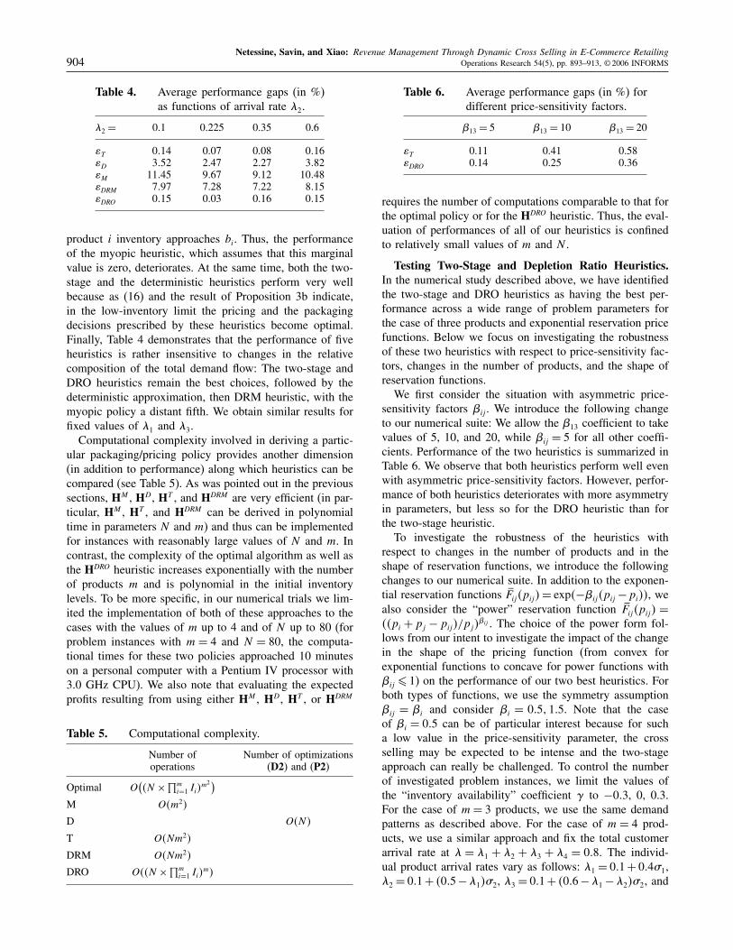
Table 2. Average performance gaps (in %)as functions of ER price.
7= 0.2 0.5 0.8
5T 0.05 0.13 0�185D 0.91 2.74 5�835M 2.63 9.38 19�875DRM 1.61 6.72 14�925DRO 0.08 0.15 0�20
the DRM heuristic occupies an intermediate place betweenthe myopic and the deterministic heuristics in terms of itsperformance. As expected, in many cases revenue losseswhen we use the myopic heuristic are remarkably large.This observation underscores the importance of a goodmatch between packaging and pricing decisions: “Deple-tion ratio” packaging, being near-optimal when coupledwith best-match pricing, loses its effectiveness when cou-pled with myopic pricing.Next, we report the results of the sensitivity analysis
with respect to the magnitude of the ER premium relativeto the product price 7 (Table 2), the inventory availabilitycoefficient 1 (Table 3), and the composition of total cus-tomer demand (Table 4). The values of 5i reported in thesetables refer to the averages over problem instances in whichthe relevant problem parameter is fixed. For example, inTable 2, the upper left value 0.05 refers to the averageof the relative performance gap for the two-stage heuristicover 2,240 problem instances with 7= 0�2.HT and HDRO heuristics are consistently producing
near-optimal performance for a wide range of problemparameters, while the performance of heuristics HM , HD,and HDRM changes in a predictable manner as problemparameters vary. For example, when the magnitude of theER price relative to the selling price of the single prod-uct 7 is small, getting additional inventory is nearly cost-free. Not surprisingly, as Table 2 indicates, HM , HD, andHDRM perform well for small values of 7. Furthermore, asTable 3 shows, when product inventory levels are high, themarginal value of an extra unit of inventory for any prod-uct is small, and all five heuristics perform well. In fact,as (16) and the result of Proposition 3b indicate, for highinventory levels both the two-stage and the deterministicheuristics coincide with the myopic heuristic, which, inturn, becomes optimal. On the other hand, when productinventory is low, the marginal value of an extra unit of
Table 3. Average performance gaps (in %) as functionsof inventory availability.
1 = −0�8 −0�3 0 0.3 0.8
5T 0�03 0�14 0�20 0.15 0.085D 0�16 2�40 7�44 3.97 1.845M 18�47 11�50 10�18 7.50 5.485DRM 17�44 9�87 6�56 3.44 1.445DRO 0�00 0�01 0�08 0.35 0.26
Netessine, Savin, and Xiao: Revenue Management Through Dynamic Cross Selling in E-Commerce Retailing904 Operations Research 54(5), pp. 893–913, © 2006 INFORMS
Table 4. Average performance gaps (in %)as functions of arrival rate �2.
�2 = 0.1 0.225 0.35 0.6
5T 0�14 0.07 0.08 0�165D 3�52 2.47 2.27 3�825M 11�45 9.67 9.12 10�485DRM 7�97 7.28 7.22 8�155DRO 0�15 0.03 0.16 0�15
product i inventory approaches bi. Thus, the performanceof the myopic heuristic, which assumes that this marginalvalue is zero, deteriorates. At the same time, both the two-stage and the deterministic heuristics perform very wellbecause as (16) and the result of Proposition 3b indicate,in the low-inventory limit the pricing and the packagingdecisions prescribed by these heuristics become optimal.Finally, Table 4 demonstrates that the performance of fiveheuristics is rather insensitive to changes in the relativecomposition of the total demand flow: The two-stage andDRO heuristics remain the best choices, followed by thedeterministic approximation, then DRM heuristic, with themyopic policy a distant fifth. We obtain similar results forfixed values of �1 and �3.Computational complexity involved in deriving a partic-
ular packaging/pricing policy provides another dimension(in addition to performance) along which heuristics can becompared (see Table 5). As was pointed out in the previoussections, HM , HD, HT , and HDRM are very efficient (in par-ticular, HM , HT , and HDRM can be derived in polynomialtime in parameters N and m) and thus can be implementedfor instances with reasonably large values of N and m. Incontrast, the complexity of the optimal algorithm as well asthe HDRO heuristic increases exponentially with the numberof products m and is polynomial in the initial inventorylevels. To be more specific, in our numerical trials we lim-ited the implementation of both of these approaches to thecases with the values of m up to 4 and of N up to 80 (forproblem instances with m = 4 and N = 80, the computa-tional times for these two policies approached 10 minuteson a personal computer with a Pentium IV processor with3.0 GHz CPU). We also note that evaluating the expectedprofits resulting from using either HM , HD, HT , or HDRM
Table 5. Computational complexity.
Number of Number of optimizationsoperations (D2) and (P2)
Optimal O(�N ×∏m
i=1 Ii�m2)
M O�m2�
D O�N�
T O�Nm2�
DRM O�Nm2�
DRO O��N ×∏mi=1 Ii�
m�
Table 6. Average performance gaps (in %) fordifferent price-sensitivity factors.
�13 = 5 �13 = 10 �13 = 20
5T 0.11 0.41 0.585DRO 0.14 0.25 0.36
requires the number of computations comparable to that forthe optimal policy or for the HDRO heuristic. Thus, the eval-uation of performances of all of our heuristics is confinedto relatively small values of m and N .
Testing Two-Stage and Depletion Ratio Heuristics.In the numerical study described above, we have identifiedthe two-stage and DRO heuristics as having the best per-formance across a wide range of problem parameters forthe case of three products and exponential reservation pricefunctions. Below we focus on investigating the robustnessof these two heuristics with respect to price-sensitivity fac-tors, changes in the number of products, and the shape ofreservation functions.We first consider the situation with asymmetric price-
sensitivity factors �ij . We introduce the following changeto our numerical suite: We allow the �13 coefficient to takevalues of 5, 10, and 20, while �ij = 5 for all other coeffi-cients. Performance of the two heuristics is summarized inTable 6. We observe that both heuristics perform well evenwith asymmetric price-sensitivity factors. However, perfor-mance of both heuristics deteriorates with more asymmetryin parameters, but less so for the DRO heuristic than forthe two-stage heuristic.To investigate the robustness of the heuristics with
respect to changes in the number of products and in theshape of reservation functions, we introduce the followingchanges to our numerical suite. In addition to the exponen-tial reservation functions �Fij�pij �= exp�−�ij�pij −pi��, wealso consider the “power” reservation function �Fij�pij � =��pi + pj − pij�/pj��ij . The choice of the power form fol-lows from our intent to investigate the impact of the changein the shape of the pricing function (from convex forexponential functions to concave for power functions with�ij � 1) on the performance of our two best heuristics. Forboth types of functions, we use the symmetry assumption�ij = �i and consider �i = 0�5�1�5. Note that the caseof �i = 0�5 can be of particular interest because for sucha low value in the price-sensitivity parameter, the crossselling may be expected to be intense and the two-stageapproach can really be challenged. To control the numberof investigated problem instances, we limit the values ofthe “inventory availability” coefficient 1 to −0�3, 0, 0.3.For the case of m= 3 products, we use the same demandpatterns as described above. For the case of m = 4 prod-ucts, we use a similar approach and fix the total customerarrival rate at � = �1 + �2 + �3 + �4 = 0�8. The individ-ual product arrival rates vary as follows: �1 = 0�1+ 0�461,�2 = 0�1+ �0�5−�1�62, �3 = 0�1+ �0�6−�1−�2�62, and

Netessine, Savin, and Xiao: Revenue Management Through Dynamic Cross Selling in E-Commerce RetailingOperations Research 54(5), pp. 893–913, © 2006 INFORMS 905
Table 7. Average (and maximum) performance gaps(in %) for two-stage and DRO heuristics.
Two-stage Exponential RF Power RF
3 products 0.13 (0.69) 0.24 (6.98)4 products 0.86 (9.05) 1.09 (7.08)
DRO Exponential RF Power RF
3 products 0.16 (1.08) 0.16 (1.94)4 products 0.46 (3.01) 0.25 (2.29)
�4 = 0�8−�1−�2−�3, where 61, 62, and 63 take values of0, 0.5, and 1. Hence, in this case we allow 27 possible com-binations of arrival rates, which, like the numerical suiteused in the previous section, cover all essential scenariosfor a four-way splitting of the total demand: “mostly single-product arrivals,” “mostly two-product arrivals,” “mostlythree-product arrivals,” and “closely-valued demands.” Theremaining problem parameters were set in the same wayas in the numerical study above. In total, we test 23 ×7× 3× 3= 504 problem instances for m= 3 products and23×27×3×3= 1�944 problem instances for m= 4 prod-ucts. The results of the numerical runs are presented inTable 7.We note that, due to changes in our test suite, the devi-
ations for the case of the exponential reservation functionand m = 3 products differ somewhat from those in theprevious section. We observe that both heuristics, on aver-age, show quite a high degree of robustness with respectto changes in the reservation function and the numberof products. This conclusion is especially valid for theDRO heuristic, which retains near-optimal performanceeven in the worst-case scenarios. In contrast, the two-stageapproach appears to lose its worst-case effectiveness whenthe number of products is increased or the shape of thereservation function is changed, or both. It is interestingto note that the worst-case performance of the two-stageheuristic is observed in problem instances with �i = 0�5and 7 = 0�8, i.e., the instances in which (1) consumersare willing to accept high package prices (for both typesof reservation functions), and (2) the out-of-stock productsare costly to replenish. It is intuitive that the heuristic thatneglects future cross-selling opportunities does not performwell in cases in which cross selling is readily acceptedby customers. This performance gap opens up dramaticallywhen the number of cross-selling choices for each productis increased from 2 (m= 3) to 3 (m= 4). The high cost ofreplenishment further accentuates the profit loss resultingfrom the use of an ineffective cross-selling approach.The ultimate choice between the DRO and the two-stage
heuristics may depend on the specific features of the busi-ness environment in which the firm operates. On the onehand, if the nature of the firm’s inventory allows it to limitthe number of likely complements for each product to two,the firm may be advised to use the two-stage approach aslong as its customers are relatively sensitive to package
prices: The pricing policies under the two-stage approachare much easier to compute than those under the DROheuristic (which requires solving a number of optimiza-tion problems at each decision epoch). On the other hand,the DRO heuristic may be a much more effective policyin cases in which the number of products is high or theestimated customer price sensitivity for product packagesis low.
4. The Lost-Sales ModelAlthough in some cases it is possible to procure an out-of-stock product, in a variety of situations this might proveimpossible or too costly. For example, when a retailer crosssells travel services, there might not be seats available onthe requested route. Hence, it will be necessary to denythe customer’s request. To address this issue, we consideran alternative setting in which there is no opportunity toreplenish inventory and a customer request is simply deniedin the case of a stockout. As in the previous section, it isconvenient to introduce the sets of indices An to denoteproducts that have at least one unit of inventory at thebeginning of the nth decision epoch. Then, under the LSModel, the generalization of (1) is given by
Vn�I�=∑i∈An�i maxj �=i� j∈An
(maxpij�Fij �pij ��pi+Vn+1�I− ei��
+ �Fij�pij ��pij +Vn+1�I− ei− ej ���)
+(1− ∑
i∈An�i
)Vn+1�I�� (22)
As (22) indicates, the “lost-sales” feature of the inventorydynamics is reflected in the fact that the set of productindices that actively participate in the DP transformationon the right-hand side of (1) “shrinks” as time passes.
4.1. Dynamic Pricing Under Static Packaging
As we indicated earlier, the LS Model possesses few struc-tural properties. However, the two-product case is some-what more amenable to analysis. Hence, we begin ouranalysis with this simple case. Under the LS Model, whena company runs out of inventory for one of the products,we obtain
Vn�I1�0�
= �1�p1 +Vn+1�I1 − 1�0��+ �1−�1�Vn+1�I1�0� (23)
for I1 � 1, n= 1� � � � �N , and
Vn�0� I2�
= �2�p2 +Vn+1�0� I2 − 1��+ �1−�2�Vn+1�0� I2� (24)
for I2 � 1, n= 1� � � � �N . In addition, when the inventoriesof both products are depleted, we have
Vn�0�0�= 0� n= 1� � � � �N � (25)
Netessine, Savin, and Xiao: Revenue Management Through Dynamic Cross Selling in E-Commerce Retailing906 Operations Research 54(5), pp. 893–913, © 2006 INFORMS
Using induction over the time index n, we can formalizethe structural properties of the LS Model in a two-productcase:
Proposition 5. (a) The optimal expected revenue Vn�I1� I2�is a nondecreasing function of I1 and I2, respectively, forany n= 1� � � � �N :
Vn�I1 + 1� I2�−Vn�I1� I2�� 0�
Vn�I1� I2 + 1�−Vn�I1� I2�� 0�(26)
(b) The optimal expected revenue Vn�I1� I2� is a super-modular function of �I1� I2� for any n= 1� � � � �N :
Vn�I1 + 1� I2 + 1�−Vn�I1� I2 + 1�
� Vn�I1 + 1� I2�−Vn�I1� I2�� (27)
(c) The optimal package price p∗ij �I1� I2� n� is nonde-creasing in Ii for �i� j�= �1�2� and �2�1�:p∗12�I1 + 1� I2� n�� p
∗12�I1� I2� n�� n= 1� � � � �N �
p∗21�I1� I2 + 1� n�� p∗21�I1� I2� n�� n= 1� � � � �N �(28)
Proof. See the technical online appendix.
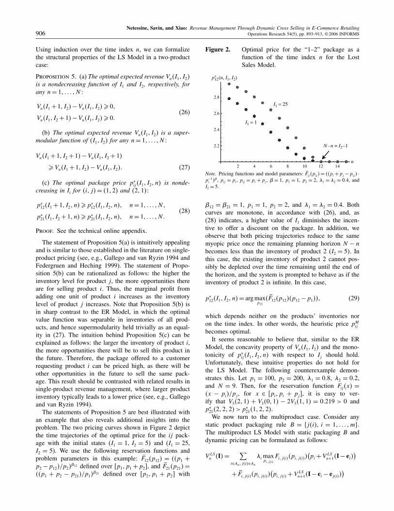
The statement of Proposition 5(a) is intuitively appealingand is similar to those established in the literature on single-product pricing (see, e.g., Gallego and van Ryzin 1994 andFedergruen and Heching 1999). The statement of Propo-sition 5(b) can be rationalized as follows: the higher theinventory level for product j , the more opportunities thereare for selling product i. Thus, the marginal profit fromadding one unit of product i increases as the inventorylevel of product j increases. Note that Proposition 5(b) isin sharp contrast to the ER Model, in which the optimalvalue function was separable in inventories of all prod-ucts, and hence supermodularity held trivially as an equal-ity in (27). The intuition behind Proposition 5(c) can beexplained as follows: the larger the inventory of product i,the more opportunities there will be to sell this product inthe future. Therefore, the package offered to a customerrequesting product i can be priced high, as there will beother opportunities in the future to sell the same pack-age. This result should be contrasted with related results insingle-product revenue management, where larger productinventory typically leads to a lower price (see, e.g., Gallegoand van Ryzin 1994).The statements of Proposition 5 are best illustrated with
an example that also reveals additional insights into theproblem. The two pricing curves shown in Figure 2 depictthe time trajectories of the optimal price for the ij pack-age with the initial states �I1 = 1� I2 = 5� and (I1 = 25,I2 = 5). We use the following reservation functions andproblem parameters in this example: �F12�p12� = ��p1 +p2 −p12�/p2��12 defined over �p1� p1 +p2�, and �F21�p21�=��p1 + p2 − p21�/p1��21 defined over �p2� p1 + p2� with
Figure 2. Optimal price for the “1–2” package as afunction of the time index n for the LostSales Model.
*p12(n, I1, I2)
I1 = 25
I1 = 1
N–n = I2–1
n2 4 6 8 10 12 14
2.8
2.6
2.4
2.2
Note. Pricing functions and model parameters: �Fij �pij �= ��pi+pj −pij � ·p−1i �
�, pij = pi, pij = pi + pj , �= 1, p1 = 1, p2 = 2, �1 = �2 = 0�4, andI2 = 5.
�12 = �21 = 1, p1 = 1, p2 = 2, and �1 = �2 = 0�4. Bothcurves are monotone, in accordance with (26), and, as(28) indicates, a higher value of I1 diminishes the incen-tive to offer a discount on the package. In addition, weobserve that both pricing trajectories reduce to the samemyopic price once the remaining planning horizon N − nbecomes less than the inventory of product 2 (I2 = 5�. Inthis case, the existing inventory of product 2 cannot pos-sibly be depleted over the time remaining until the end ofthe horizon, and the system is prompted to behave as if theinventory of product 2 is infinite. In this case,
p∗12�I1� I2� n�= argmaxp12� �F12�p12��p12 −p1��� (29)
which depends neither on the products’ inventories noron the time index. In other words, the heuristic price pMijbecomes optimal.It seems reasonable to believe that, similar to the ER
Model, the concavity property of Vn�I1� I2� and the mono-tonicity of p∗ij �I1� I2� n� with respect to Ij should hold.Unfortunately, these intuitive properties do not hold forthe LS Model. The following counterexample demon-strates this. Let p1 = 100, p2 = 200, �1 = 0�8, �2 = 0�2,and N = 9. Then, for the reservation function Fij�x� =�x − pi�/pj , for x ∈ �pi� pi + pj�, it is easy to ver-ify that V3�2�1� + V3�0�1� − 2V3�1�1� = 0�219 > 0 andp∗21�2�2�2� > p
∗21�1�2�2�.
We now turn to the multiproduct case. Consider anystatic product packaging rule B = �j�i�� i = 1� � � � �m�.The multiproduct LS Model with static packaging B anddynamic pricing can be formulated as follows:
V LSn �I�=∑
i∈An� j�i�∈An�imax
pi� j�i�Fi� j�i��pi� j�i��
(pi+V LSn+1�I− ei�
)+ �Fi� j�i��pi� j�i��
(pi� j�i�+V LSn+1�I− ei− ej�i��
)
Netessine, Savin, and Xiao: Revenue Management Through Dynamic Cross Selling in E-Commerce RetailingOperations Research 54(5), pp. 893–913, © 2006 INFORMS 907
+ ∑i∈An� j�i�An
�i�pi+Vn+1�I− ei��
+(1− ∑
i∈An�i
)V LSn+1�I�� (30)
In the multiproduct case, the few properties possessed bythe two-product LS Model vanish. For example, the super-modularity of the optimal value function no longer holds,and the LS Model retains only the monotonicity of optimalrevenues with the product inventory levels, which can beestablished using the induction over time index n:
Proposition 6. The optimal expected revenue is nonde-creasing in the inventory level, i.e., V LSn �I + ei� � V
LSn �I�
for i= 1� � � � �m and n= 1� � � � �N .
Proof. See the technical online appendix.
4.2. Heuristic Approaches
Because even the standalone dynamic pricing problemunder the LS Model is rather intractable, there is little hopeof efficiently solving the dynamic pricing/packaging prob-lem without the use of heuristics. Hence, it is desirable toknow how much we might lose by implementing a sim-ple static packaging policy. Below we derive upper andlower bounds for the expected profit under the LS Modelwith static packaging and dynamic pricing. Using these twobounds, we identify situations under which a given packag-ing configuration will lead to negligible benefits comparedwith no packaging.
Definition 2. Let Lin�I� be the function satisfying the fol-lowing recursive relation:
Lin�I�= �i�pi+Lin+1�I − 1��+ �1−�i�Lin+1�I� (31)
for I � 1, and Lin�0�= 0 for i= 1� � � � �m and n= 1� � � � �N ,while LiN+1�I�= 0.
Definition 3. Let U in�I� be the function satisfying the fol-lowing recursive relation:
U in�I�= �i�pi+U in+1�I − 1�+ �Fi� j�i��pMi� j�i���pMi� j�i�−pi��+ �1−�i�U in+1�I� (32)
for I � 1, and U in�0�= 0 for i= 1� � � � �m and n= 1� � � � �N ,while U iN+1�I�= 0.
We define Ln�I�=∑mi=1L
in�Ii� and Un�I�=
∑mi=1U
in�Ii�.
Note that Ln�I� is the expected revenue under the LS Modelwith no packaging. The following proposition uses theinduction over n to show that Ln�I� and Un�I� are a lowerbound and an upper bound, respectively, for the optimalexpected revenue V LSn �I� in the LS Model.
Proposition 7. (a) Ln�I� � V LSn �I� � Un�I� for n =1� � � � �N .
(b) For n= 1� � � � �N ,
V LSn �I�−Ln�I�Ln�I�
�max{pj�i�
pi
∣∣∣∣ i= 1� � � � �m}� (33)
Proof. See the technical online appendix.
Note that the upper bound given in Proposition 7(b)is independent of customer reservation prices and arrivalprocesses. If each product is significantly more expensivethan its packaging complement, then the bound in (33) istight, implying that the impact of the packaging decisionon expected profit is negligible relative to no packaging.Given the price of each product, we can now easily com-pute the upper bound for each packaging topology. Thus,without the demand information, we are able to identifythe packaging configurations with the tight upper bound.Consider an example in which �p1� p2� p3� = �100�10�1�and product 1 is packaged with product 2, and product 2with product 3 (product 3 is not packaged with any otherproduct). According to (33), under this packaging configu-ration, the highest possible revenue is at most 10% abovethe revenue achieved in the absence of cross selling.Even with static packaging, the computation of the
optimal price under the LS assumption requires solvingan m-dimensional DP problem (30) that is computationallychallenging for a large m. Therefore, there exists a need todevelop a simple, easy-to-implement, and effective pricingheuristic. As (30) indicates, the optimal package price canbe expressed as the maximizer of the following expression:
p∗ij �I� n�= argmaxpij
( �Fij�pij �(pij −pi+ �Vn+1�I− ei− ej �−Vn+1�I− ei��
))� (34)
A natural approximation under the above modification is touse the package prices defined by pMij in (13), essentiallyignoring the last two terms of (34). This heuristic packageprice is constant over the time horizon and is independentof the inventory level of either product. We reuse the nota-tion HM to denote this heuristic (exactly the same heuris-tic applies to the two models, ER and LS). The followingresult states that pMij is the lower bound on the optimal pricep∗ij �I� n�, and characterizes the sufficient conditions underwhich the heuristic HM is optimal:
Proposition 8. (a) The optimal price is never less than theprice determined by the heuristic HM4 p∗ij �I� n� � p
Mij for
any I and n.(b) Heuristic HM is optimal in period n when the avail-
able inventory is Ik �N + 2− n for all k= 1�2� � � � �m.
Proof. See the technical online appendix.
The proof of Proposition 8(a) utilizes the monotonicityof the value function established in Proposition 6. Propo-sition 8(b) indicates that the static pricing heuristic is opti-mal in cases in which the inventory level of every product
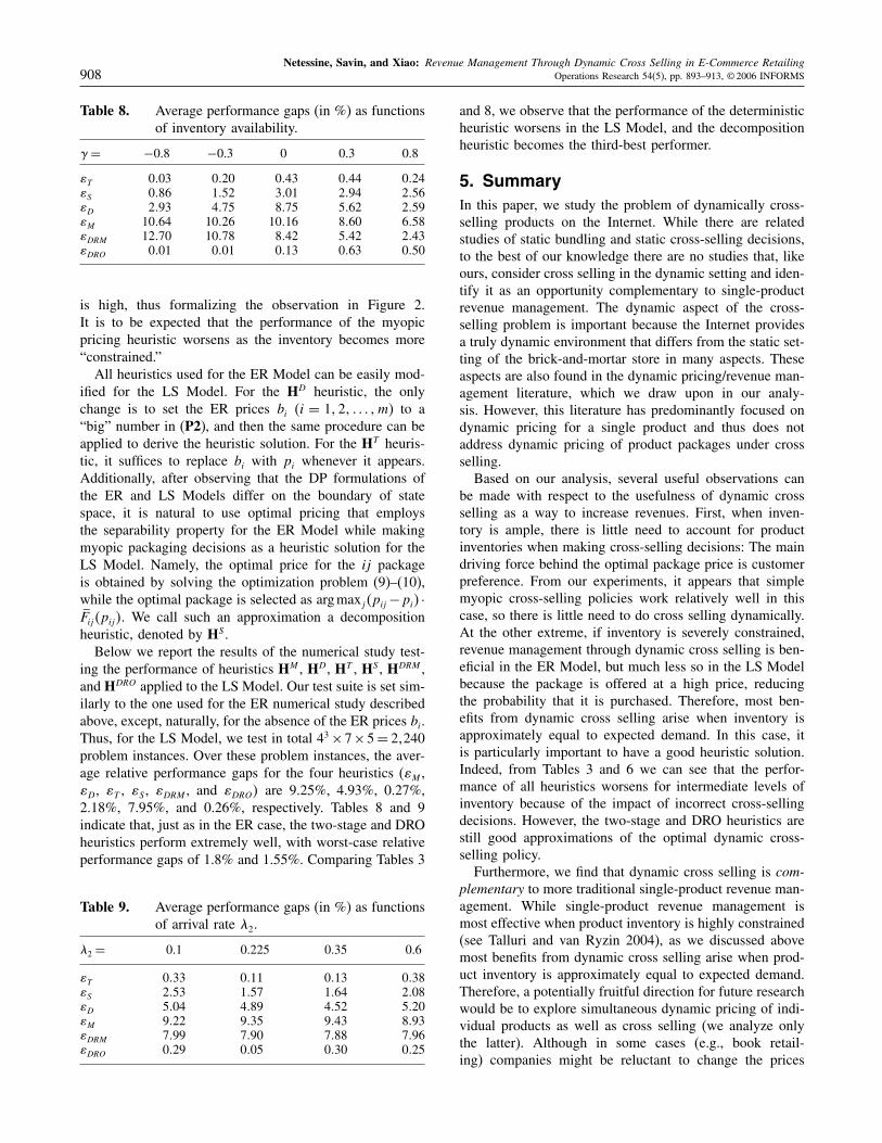
Netessine, Savin, and Xiao: Revenue Management Through Dynamic Cross Selling in E-Commerce Retailing908 Operations Research 54(5), pp. 893–913, © 2006 INFORMS
Table 8. Average performance gaps (in %) as functionsof inventory availability.
1 = −0.8 −0.3 0 0.3 0.8
5T 0�03 0�20 0�43 0�44 0�245S 0�86 1�52 3�01 2�94 2�565D 2�93 4�75 8�75 5�62 2�595M 10�64 10�26 10�16 8�60 6�585DRM 12�70 10�78 8�42 5�42 2�435DRO 0�01 0�01 0�13 0�63 0�50
is high, thus formalizing the observation in Figure 2.It is to be expected that the performance of the myopicpricing heuristic worsens as the inventory becomes more“constrained.”All heuristics used for the ER Model can be easily mod-
ified for the LS Model. For the HD heuristic, the onlychange is to set the ER prices bi (i = 1�2� � � � �m) to a“big” number in (P2), and then the same procedure can beapplied to derive the heuristic solution. For the HT heuris-tic, it suffices to replace bi with pi whenever it appears.Additionally, after observing that the DP formulations ofthe ER and LS Models differ on the boundary of statespace, it is natural to use optimal pricing that employsthe separability property for the ER Model while makingmyopic packaging decisions as a heuristic solution for theLS Model. Namely, the optimal price for the ij packageis obtained by solving the optimization problem (9)–(10),while the optimal package is selected as argmaxj �pij−pi� ·�Fij�pij �. We call such an approximation a decompositionheuristic, denoted by HS .Below we report the results of the numerical study test-
ing the performance of heuristics HM , HD, HT , HS , HDRM ,and HDRO applied to the LS Model. Our test suite is set sim-ilarly to the one used for the ER numerical study describedabove, except, naturally, for the absence of the ER prices bi.Thus, for the LS Model, we test in total 43×7×5= 2�240problem instances. Over these problem instances, the aver-age relative performance gaps for the four heuristics (5M ,5D, 5T , 5S , 5DRM , and 5DRO� are 9.25%, 4.93%, 0.27%,2.18%, 7.95%, and 0.26%, respectively. Tables 8 and 9indicate that, just as in the ER case, the two-stage and DROheuristics perform extremely well, with worst-case relativeperformance gaps of 1.8% and 1.55%. Comparing Tables 3
Table 9. Average performance gaps (in %) as functionsof arrival rate �2.
�2 = 0.1 0.225 0.35 0.6
5T 0�33 0�11 0�13 0�385S 2�53 1�57 1�64 2�085D 5�04 4�89 4�52 5�205M 9�22 9�35 9�43 8�935DRM 7�99 7�90 7�88 7�965DRO 0�29 0�05 0�30 0�25
and 8, we observe that the performance of the deterministicheuristic worsens in the LS Model, and the decompositionheuristic becomes the third-best performer.
5. SummaryIn this paper, we study the problem of dynamically cross-selling products on the Internet. While there are relatedstudies of static bundling and static cross-selling decisions,to the best of our knowledge there are no studies that, likeours, consider cross selling in the dynamic setting and iden-tify it as an opportunity complementary to single-productrevenue management. The dynamic aspect of the cross-selling problem is important because the Internet providesa truly dynamic environment that differs from the static set-ting of the brick-and-mortar store in many aspects. Theseaspects are also found in the dynamic pricing/revenue man-agement literature, which we draw upon in our analy-sis. However, this literature has predominantly focused ondynamic pricing for a single product and thus does notaddress dynamic pricing of product packages under crossselling.Based on our analysis, several useful observations can
be made with respect to the usefulness of dynamic crossselling as a way to increase revenues. First, when inven-tory is ample, there is little need to account for productinventories when making cross-selling decisions: The maindriving force behind the optimal package price is customerpreference. From our experiments, it appears that simplemyopic cross-selling policies work relatively well in thiscase, so there is little need to do cross selling dynamically.At the other extreme, if inventory is severely constrained,revenue management through dynamic cross selling is ben-eficial in the ER Model, but much less so in the LS Modelbecause the package is offered at a high price, reducingthe probability that it is purchased. Therefore, most ben-efits from dynamic cross selling arise when inventory isapproximately equal to expected demand. In this case, itis particularly important to have a good heuristic solution.Indeed, from Tables 3 and 6 we can see that the perfor-mance of all heuristics worsens for intermediate levels ofinventory because of the impact of incorrect cross-sellingdecisions. However, the two-stage and DRO heuristics arestill good approximations of the optimal dynamic cross-selling policy.Furthermore, we find that dynamic cross selling is com-
plementary to more traditional single-product revenue man-agement. While single-product revenue management ismost effective when product inventory is highly constrained(see Talluri and van Ryzin 2004), as we discussed abovemost benefits from dynamic cross selling arise when prod-uct inventory is approximately equal to expected demand.Therefore, a potentially fruitful direction for future researchwould be to explore simultaneous dynamic pricing of indi-vidual products as well as cross selling (we analyze onlythe latter). Although in some cases (e.g., book retail-ing) companies might be reluctant to change the prices

Netessine, Savin, and Xiao: Revenue Management Through Dynamic Cross Selling in E-Commerce RetailingOperations Research 54(5), pp. 893–913, © 2006 INFORMS 909
of individual products dynamically, in other applications(especially travel services) this extension might be plausi-ble. We hope that future research will consider this option.We believe that research in the area of dynamic cross
selling has the potential to make an important practicalimpact. According to several experts, dynamic cross sellingof nonair elements of a travel package with airline ticketshas the potential to generate large incremental revenues inan industry plagued by low margins (see Feldman 2003).Web merchants who analyze revenue gains from cross sell-ing report a 5% increase on average (see Peters 2004).Although early experiments with dynamic pricing of indi-vidual products on the Internet have failed (see the exampleof Amazon.com in CIO Magazine 2000) due to poor per-ception by customers, dynamic cross selling seems to beflourishing. The reason might be that customers perceivea package as “fairly” priced as long as it is not pricedabove the sum of its components, and moreover, cross sell-ing offers may provide valuable information to customersby introducing them to new products. While Internet com-panies are in need of easy-to-implement algorithms fordynamic cross selling, operations research currently offerslittle help in this respect. In particular, efficient algorithmsare needed to deal with multidimensional cross-sellingproblems that otherwise are too computationally intensive.Some obvious extensions of our work may include allowingindividual product prices to be adjusted dynamically, allow-ing multiple packages to be offered to the same customerand letting customers self-select a package. A study of therelated practice of up selling customers to products withhigher revenues offers the possibility of fruitful researchas well.
AppendixFor the proofs of some propositions, we need an additionalresult:
Lemma A1. Let gij�x� = maxy� �Fij�y��y − x��, where 1 �i �= j �m.(a) For any x1 � 0 and x2 � 0,
max�0� x2 − x1�� gij�x1�− gij�x2��min�0� x2 − x1�� (A1)
(b) For any x1 � x2 � 0, let yk be the maximizer ofgij�xk� (k= 1�2). Then, y1 � y2.
Proof of Lemma A1. Let yk be the maximizer of gij�xk��k = 1�2�. We consider two cases: x1 � x2 and x1 � x2.If x1 � x2, then by definition, gij�x2� = �Fij�y2��y2 − x2� ��Fij�y1��y1 − x2� � �Fij�y1��y1 − x1� = gij�x1� � �Fij�y2� ·�y2 − x1�. This yields 0 � gij�x2� − gij�x1� � �Fij�y2� ·�x1 − x2� � x1 − x2 and �Fij�y1� � �Fij�y2�, i.e., y1 � y2. Ifx1 � x2, by symmetry, we have 0 � gij�x1� − gij�x2� �x2 − x1. Combining these two cases, we obtain (A1). �
Proof of Proposition 1. The statement trivially holds forn = N + 1. Using induction, suppose that for some n =1� � � � �N ,
Vn+1�I�=m∑i=1Gin+1�Ii�� (A2)
We need to prove that Vn�I�=∑mi=1G
in�Ii�.
Vn�I�=∑
i∈An� j�i�∈An�i
(pi+Vn+1�I− ei�+max
pi� j�i�� �Fi� j�i��pi� j�i��
·�pi�j�i�−pi+Vn+1�I−ei−ej�i��−Vn+1�I−ei���)
+ ∑i∈An� j�i�An
�i
(pi+Vn+1�I− ei�
+maxpi� j�i�
� �Fi� j�i��pi� j�i���pi� j�i�−pi− bj�i���)
+ ∑iAn�j�i�∈An
�i
(pi−bi+Vn+1�I�+max
pi�j�i�
�Fi�j�i��pi�j�i��
· �pi� j�i�−pi+Vn+1�I− ej�i��−Vn+1�I��)
+ ∑iAn�j�i�An
�i
(pi−bi+Vn+1�I�+max
pi�j�i�
�Fi�j�i��pi�j�i��
·�pi�j�i�−pi−bj�i��)+(1−
m∑i=1�i
)Vn+1�I�
= ∑i∈An� j�i�∈An
�i
(pi+Gin+1�Ii− 1�−Gin+1�Ii�
+maxpi� j�i�
�Fi� j�i��pi� j�i��(pi� j�i�−pi+Gj�i�n+1�Ij�i�− 1�
−Gj�i�n+1�Ij�i��))
+ ∑i∈An� j�i�An
�i
(pi+Gin+1�Ii− 1�−Gin+1�Ii�
+maxpi� j�i�
�Fi� j�i��pi� j�i���pi� j�i�−pi− bj�i��)
+ ∑iAn� j�i�∈An
�i
(pi− bi+max
pi� j�i�
�Fi� j�i��pi� j�i��
· (pi� j�i�−pi+Gj�i�n+1�Ij�i�− 1�−Gj�i�n+1�Ij�i��))
+ ∑iAn� j�i�An
�i
(pi− bi+max
pi� j�i�
�Fi� j�i��pi� j�i��
·�pi�j�i�−pi−bj�i��)+
m∑i=1Gin+1�Ii� �from (A2)�
=m∑i=1Gin�Ii� �from (9)�� �
Proof of Proposition 3. (a) Following the standardLagrangian procedure to derive the dual function q�*�<�,

Netessine, Savin, and Xiao: Revenue Management Through Dynamic Cross Selling in E-Commerce Retailing910 Operations Research 54(5), pp. 893–913, © 2006 INFORMS
we have
q�*�<�= maxq�0� y�0� pij�0
L�p�q� y�*�<�
= maxq�0�y�0�pij�0
{ m∑i=1
∑j �=i�j(qji �Fji�pji��pji−pj�−
m∑i=1biyi
+m∑i=1*i
[yi+ Ii−�i( −
∑j �=i�j(qji �Fji�pji�
]
+m∑i=1<i
(1−∑
j �=iqij
)}
= maxq�0�y�0�pij�0
{ m∑i=1
∑j �=i��j( �Fji�pji��pji−pj−*i�−<j�
·qji+m∑i=1�*i−bi�yi+
m∑i=1�*i�Ii−�i(�+<i�
}
= maxq�0�y�0
{ m∑i=1
∑j �=i��j(Hji�*i�−<j�qji+
m∑i=1�*i−bi�yi
+m∑i=1�*i�Ii−�i(�+ <i�
}� (A3)
where the last equation follows from the definition ofHji�*i�. Define Dq = ��*�<� � q�*�v� <+��. It is easy tosee from (A3) that Dq = ��*�<� � �j(Hji�*i�− vj � 0 fori �= j and *i � bi�, and q�*�<�=
∑mi=1�*i�Ii − �i(�+ <i�
for �*�<� ∈Dq . Hence, the dual problem (D2) can be for-mulated as follows:
min*i� vj
4 q�*� v�=m∑i=1�*i�Ii−�i(�+ vi�
s.t. �j(Hji�*i�� vj for i �= j�0�*i � bi for i= 1�2� � � � �m�
To show that the above constraint set is convex, it suf-fices to show that Hji�x� is convex for every pair i �= j .Recall that Hji�x�=maxpji �
�Fji�pji��pji − pj − x��. Denotethe maximizer of �Fji�pji��pji − pj − x� by pji�x� . Then,from the first-order condition, we have
d �Fji�pji��pji−pj − x�dpji
∣∣∣∣pji=pji�x�
= 0� (A4)
Taking the derivative of Hji�x�, we have
dHji�x�
dx= d
�Fji�pji��pji−pj − x�dpji
∣∣∣∣pji=pji�x�
dpji�x�
dx
− �Fji�pji�x��=− �Fji�pji�x��� (A5)
where the last equality follows from (A4). Hence,d2Hji�x�/dx
2 = �dF �x�/dx��dpji�x�/dx� � 0, which fol-lows from Lemma A1(b) and the fact that F �x� is a cumu-lative distribution function. This proves Proposition 3(a).
(b) It is easy to ensure that the constraint set of (D2)is compact by imposing a finite bound on v. Hence, theWeierstrass Theorem ensures the existence of the optimalsolution to (D2). Denote the optimal solution to (D2) by�*∗� <∗�. It is easy to verify that any solution to (D2) isregular. It follows from the KKT necessary conditions thatthere exist �q∗ij � and �y
∗i � satisfying the following KKT con-
ditions of (D2) (note that (A4) is used in deriving the KKTconditions):(y∗i + Ii−�i( −
∑j �=i�j(q
∗ji�Fji�pji�*∗
i ��
)*∗i = 0
for i= 1�2� � � � �m�∑j �=iq∗ij = 1 for i= 1�2� � � � �m� (A6)
�*∗i − bi�y∗i = 0 for i= 1�2� � � � �m� (A7)
��j(Hji�*∗i �− v∗j �q∗ji = 0� (A8)
y∗i � 0 for i= 1�2� � � � �m� (A9)
y∗i �−Ii+�i( +∑j �=i�j(q
∗ji�Fji�pji�*∗
i ��
for i= 1�2� � � � �m� (A10)
q∗ij � 0 for i �= j� (A11)
Define p∗ji = pji�*∗i �. Note that (A6), (A9), (A10), and
(A11) are the four constraints of (P2). Hence, ��q∗ij �,�y∗i �� �p
∗ij �� is a feasible solution to (P2) and yields the fol-
lowing objective value:
m∑i=1
∑j �=i�j(q
∗ji�Fji�p∗ji��p∗ji−pj�−
m∑i=1biy
∗i
=m∑i=1
∑j �=i�j(q
∗ji�Fji�p∗ji��p∗ji−pj�−
m∑i=1*∗i y
∗i (by (A7))
=m∑i=1
∑j �=i�j(q
∗ji�Fji�p∗ji��p∗ji−pj −*∗
i �
+m∑i=1*∗i �Ii−�i(� (by (A6))
=m∑i=1
∑j �=i�j(q
∗jiHji�*
∗i �+
m∑i=1*∗i �Ii−�i(�(by definition of Hji�x��
=m∑i=1
∑j �=iq∗jiv
∗j +
m∑i=1*∗i �Ii−�i(� (by (A8))
=m∑i=1v∗i +
m∑i=1*∗i �Ii−�i(� (by (A6))�
which is equal to the optimal value of the dual problem.By weak duality, ��q∗ij �, �y
∗i �� �p
∗ij �� is an optimal solution
to (P2). This proves Proposition 3(b)(i), One can obtainthe optimal solution to (P2) using the above KKT condi-tions. An alternative way is to solve a linear programming
Netessine, Savin, and Xiao: Revenue Management Through Dynamic Cross Selling in E-Commerce RetailingOperations Research 54(5), pp. 893–913, © 2006 INFORMS 911
problem (P2) with pij being replaced by p∗ij . This provesProposition 3(b)(ii). �
Proof of Proposition 4. Because q < p+b, it is subopti-mal to choose a product with zero inventory as a packagingcomplement. Therefore, the dynamic packaging problemreduces to
Vn�I�=∑i∈A�I�
�(�1−1��p+Vn+1�I− ei��
+ maxj �=i� j∈A�I�
1�q+Vn+1�I− ei− ej ��)
+ ∑iA�I�
�(�1−1��p− b+Vn+1�I��+ maxj �=i� j∈A�I�
1�q− b+Vn+1�I− ej ��)
+ �1−m��Vn+1�I�� (A12)
where A�I� denotes products that have at least one unit ofinventory at the beginning of the nth decision epoch whenthe inventory is I. The boundary condition is VN+1�I�= 0.To prove the optimality of the DR packaging, we need toshow that Vn�I− ek�� Vn�I− el� (because �i = �) for anyI = �I1� I2� � � � � Im� with Ik � Il � 1 and any n = 1� � � � �N + 1. First, from the boundary condition, this inequalitytrivially holds when n=N + 1. By induction, suppose thatit also holds up to some n+ 1, i.e.,
Vs�I− ek�� Vs�I− el� for any I= �I1� I2� � � � � Im�with Ik � Il � 1 and s = n+ 1� � � � �N + 1� (A13)
We prove the desired result for two separate cases: Ik =Il = 1 and Ik > Il = 1 (the proof for the case of Ik� Il > 1follows similar steps).Case 1. Ik = Il = 1. Define B = �i � i �= k� l and Ii > 0�
and C = �i � i �= k� l and Ii = 0�. Then, A�I− ek�= B ∪ �l�and A�I− el�= B∪ �k�. Note that for any i ∈ B, by (A13),we have
maxj �=i� j∈B
1�q+Vn+1�I− ei− ej−ek��� maxj �=i� j∈B
1�q+Vn+1�I− ei− ej−el���
which implies that
maxj �=i� j∈B∪�l�
1�q+Vn+1�I− ei− ej−ek��� maxj �=i� j∈B∪�k�
1�q+Vn+1�I− ei− ej−el��� (A14)
Similarly, for any i ∈C, by (A13), we have
maxj �=i� j∈B∪�l�
1�q− b+Vn+1�I− ej−ek��� maxj �=i� j∈B∪�k�
1�q− b+Vn+1�I− ej−el��� (A15)
By (A12), we have
Vn�I− ek�
=∑i∈B�(�1−1��p+Vn+1�I− ei−ek��+ maxj �=i� j∈B∪�l�
1�q+Vn+1�I− ei− ej−ek��)
+�(�1−1��p+Vn+1�I− el−ek��
+ maxj �=l� j∈B∪�l�
1�q+Vn+1�I− el− ej−ek��)
+∑i∈C�(�1−1��p− b+Vn+1�I− ek��
+ maxj �=i� j∈B∪�l�
1�q− b+Vn+1�I− ej−ek��)
+�(�1−1��p− b+Vn+1�I− ek��
+ maxj �=k� j∈B∪�l�
1�q− b+Vn+1�I− ej−ek��)
+ �1−m��Vn+1�I− ek�
�∑i∈B�(�1−1��p+Vn+1�I− ei−el��+ maxj �=i� j∈B∪�k�
1�q+Vn+1�I− ei− ej−el��)
+�(�1−1��p+Vn+1�I− ek−el��
+ maxj �=l� j∈B∪�k�
1�q+Vn+1�I− ek− ej−el��)
+∑i∈C�(�1−1��p− b+Vn+1�I− el��
+ maxj �=i� j∈B∪�k�
1�q− b+Vn+1�I− ej−el��)
+�(�1−1��p− b+Vn+1�I− el��
+ maxj �=l� j∈B∪�k�
1�q− b+Vn+1�I− ej−el��)
+�1−m��Vn+1�I−el� (by (A13), (A14), and (A15))
= Vn�I− el��
Case 2. Ik > Il = 1. Note that for any n = 1�2� � � � �N ,i = 1�2� � � � �m, and inventory vector I, we haveVn�I− ei�+ b � Vn�I�, which together with (A13) impliesthat
Vn+1�I− ek−ek��−b+Vn+1�I− el�� (A16)
and for any j ∈ B,
Vn+1�I− ek− ej−ek��−b+Vn+1�I− ej−el�� (A17)
Vn�I− ek�
=∑i∈B�(�1−1��p+Vn+1�I− ei−ek��+ maxj �=i� j∈B∪�k� l�
1�q+Vn+1�I− ei− ej−ek��)

Netessine, Savin, and Xiao: Revenue Management Through Dynamic Cross Selling in E-Commerce Retailing912 Operations Research 54(5), pp. 893–913, © 2006 INFORMS
+�(�1−1��p+Vn+1�I− el−ek��
+ maxj �=l� j∈B∪�k� l�
1�q+Vn+1�I− el− ej−ek��)
+�(�1−1��p+Vn+1�I− ek−ek��
+ maxj �=k� j∈B∪�k� l�
1�q+Vn+1�I− ek− ej−ek��)
+∑i∈C�(�1−1��p− b+Vn+1�I− ek��
+ maxj �=i� j∈B∪�k� l�
1�q− b+Vn+1�I− ej−ek��)
+ �1−m��Vn+1�I− ek�
�∑i∈B�(�1−1��p+Vn+1�I− ei−el��+ maxj �=i� j∈B∪�k�
1�q+Vn+1�I− ei− ej−el��)
+�(�1−1��p+Vn+1�I− ek−el��
+ maxj �=l� j∈B∪�k�
1�q+Vn+1�I− ek− ej−el��)
+∑i∈C�(�1−1��p− b+Vn+1�I− el��
+ maxj �=i� j∈B∪�k�
1�q− b+Vn+1�I− ej−el��)
+�(�1−1��p− b+Vn+1�I− el��
+ maxj �=l� j∈B∪�k�
1�q− b+Vn+1�I− ej−el��)
+�1−m��Vn+1�I−el� (by (A13), (A16), and (A17))
= Vn�I− el�� �
Endnotes1. At the time of this writing, Amazon.com did not offerdiscounts on book packages.2. In this respect, the choice to sell a product as part of apackage at a discount now or to sell it individually later issimilar to the standard yield management problem that iscommon for airlines.3. Such a model is consistent, for example, with a Poissonarrival process for which the probability of more than onearrival per period may be made arbitrarily small.4. The implicit assumption here is that the probability ofpurchasing a product is time invariant, while in practicethis probability may be affected by the firm’s decisions. Forexample, intensive cross selling of product j may result infewer customers buying this product in the future.5. In our analysis, we consider individual product price tobe fixed but package price to be dynamic. This approach isoften justified in practice because some Internet retailers tryto avoid dynamically changing prices of individual prod-ucts for fear of antagonizing customers (see the exam-ple of Amazon.com’s experience in CIO Magazine 2000).Alternatively, our analysis can complement the traditional
single-product revenue management literature, which stud-ies the effects of dynamically changing prices for individualproducts (see McGill and van Ryzin 1999 for a thoroughsurvey).6. A more general way to model this problem is toallow the consumer to choose simultaneously among prod-ucts i, j , and a package ij . In this case, the probabilityof selecting each of these options might depend on pi� pj ,and pij . However, our approach is plausible when product jhas a low value without product i (e.g., a hotel reservationwithout an airline ticket), and it also matches practicallyobserved applications of cross selling relatively well.7. It can be verified that after imposing a not particularlyrestrictive condition that the pricing reservation functionhas an increasing failure rate distribution, the objectivefunction is unimodal in pij .
AcknowledgmentsThe authors are grateful to the area editor Jan VanMieghem, the associate editor, and two anonymous refer-ees for suggestions that helped improve the paper. Finan-cial support from the Columbia Center for Excellence inE-business is gratefully acknowledged.
ReferencesAdams, W. J., J. L. Yellen. 1976. Commodity packaging and the burden
of monopoly. Quart. J. Econom. 90 475–498.
Adomavicius, G., A. Tuzhilin. 2002. An architecture of e-butler: Aconsumer-centric online personalization system. Internat. J. Compu-tational Intelligence Appl. 2 313–327.
Aviv, Y., A. Pazgal. 2005. A partially observed Markov decision processfor dynamic pricing. Management Sci. 51(9) 1400–1416.
Bertsimas, D. J., A. J. Mersereau, N. R. Patel. 2003. Dynamic classifica-tion of online customers. Proc. SIAM Internat. Conf. Data Mining.
Bitran, G., R. Caldentey. 2003. Commissioned paper: An overview of pric-ing models for revenue management. Manufacturing Service Oper.Management 5 203–229.
Business Week. 2004. Design your own discount gateway. (March 8).
CIO Magazine. 2000. Is dynamic pricing really so bad? (October 25).http://comment.cio.com/soundoff/102500.html.
Elmaghraby, W., P. Keskinocak. 2003. Dynamic pricing in the presence ofinventory considerations: Research overview, current practices, andfuture directions. Management Sci. 49 1287–1309.
Ernst, R., P. Kouvelis. 1999. The effect of selling packaged goods oninventory decisions. Management Sci. 45 1142–1155.
Federgruen, A., A. Heching. 1999. Combined pricing and inventory con-trol under uncertainty. Oper. Res. 47 454–475.
Federgruen, A., H. Groenevelt, H. C. Tijms. 1984. Coordinated replen-ishment in a multi-item inventory system with compound Poissondemands. Management Sci. 30 344–357.
Feldman, J. M. 2003. Package deal. Air Transport World 40(3) 40–42.
Fuerderer, R., A. Herrmann, G. Wuebker, eds. 1999. Optimal Bundling:Marketing Strategies for Improving Economic Performance. Springer,Berlin, Germany.
Gallego, G., G. van Ryzin. 1994. Optimal dynamic pricing of inventorieswith stochastic demand over finite horizons. Management Sci. 40999–1020.

Netessine, Savin, and Xiao: Revenue Management Through Dynamic Cross Selling in E-Commerce RetailingOperations Research 54(5), pp. 893–913, © 2006 INFORMS 913
Gallego, G., G. van Ryzin. 1997. A multiproduct dynamic pricing problemand its applications to network yield management. Oper. Res. 4524–41.
Hanson, W., R. K. Martin. 1990. Optimal package pricing. ManagementSci. 36 155–174.
Kamakura, W. A., M. Wedel, F. de Rosa, J. A. Mazzon. 2003. Cross-selling through database marketing: A mixed data factor analyzerfor data augmentation and prediction. Internat. J. Res. Marketing 2045–65.
Maglaras, C., J. Meissner. 2003. Dynamic pricing strategies for multi-product revenue management problems. Working paper, ColumbiaUniversity, New York.
McGill, J. I., G. van Ryzin. 1999. Revenue management: Researchoverview and prospects. Transportation Sci. 33 233–256.
Moe, W. W., P. S. Fader. 2004. Dynamic conversion behavior ate-commerce sites. Management Sci. 50 326–335.
Monahan, G. E., N. C. Petruzzi, W. Zhao. 2004. The dynamic pric-ing problem from a newsvendor perspective. Manufacturing ServiceOper. Management 6 73–91.
Nash, D., A. Sterna-Karwat. 1996. An application of DEA to measurebranch cross selling efficiency. Comput. Oper. Res. 23(4) 385–392.
Netessine, S., N. Rudi. 2006. Supply chain choice on the Internet. Man-agement Sci. 52(6) 844–864.
Padmanabhan, B., A. Tuzhilin. 2003. On the use of optimization for datamining: Theoretical interactions and eCRM opportunities. Manage-ment Sci. 49 1327–1343.
Peters, K. 2004. May we suggest? Internet Retailer (January).
Plambeck, E., A. Ward. 2003. A separation principle for assemble-to-order systems with expediting. Working paper, Stanford University,Stanford, CA.
Rao, V. R. 1993. Pricing models in marketing. J. Eliashberg, G. L. Lilien,eds. Handbooks in Operations Research and Management Science:Marketing. North-Holland, Amsterdam, The Netherlands, 517–552.
Scarf, H. 1960. The optimality of �s� S� policies in the dynamic inventoryproblem. K. Arrow, S. Karlin, P. Suppes, eds. Mathematical Modelsin Social Sciences. Stanford University Press, Stanford, CA.
Stigler, G. 1963. A note on block booking. Reprinted in Organization ofIndustry. University of Chicago Press, Chicago, IL, 165–171.
Stremersch, S., G. J. Tellis. 2002. Strategic packaging of products andprices: A new synthesis for marketing. J. Marketing 66 55–72.
Talluri, K. T., G. J. van Ryzin. 2004. The Theory and Practice of RevenueManagement. Kluwer Academic Publishers, Boston, MA.
Veinott, A. F., 1966. On the optimality of �s� S� inventory policies: Newconditions and a new proof. SIAM J. Appl. Math. 14 1067–1083.
Weigend, A. 2004. Presentation at Wharton School, University of Penn-sylvania, Philadelphia, PA, March 17.
Zhang, D., W. L. Cooper. 2005. Revenue management for parallel flightswith customer choice behavior. Oper. Res. 53(3) 415–431.
Zheng, Y.-S. 1991. A simple proof for optimality of �s� S� policies ininfinite-horizon inventory systems. J. Appl. Probab. 28 802–810.
Zheng, Y.-S. 1994. Optimal control policy for stochastic inventory systemswith Markovian discount opportunities. Oper. Res. 42 721–738.
Ziya, S., H. Ayhan, R. D. Foley. 2004. Relationship among three assump-tions in revenue management. Oper. Res. 52 804–809.