FLIGHT TRANSPORTATION LABORATORYREPORT R 92-1

Revenue Impacts of

Airline Yield Management

Chung Yu Mak

January 1992

REVENUE IMPACTS OF AIRLINE YIELD MANAGEMENT

by

Chung Yu Mak

Submitted to the Department of Civil Engineeringon January 17, 1992 in partial fulfillment

of the requirements for the Degree ofMaster of Science in Transportation

ABSTRACT

In the highly competitive airline industry today, Yield or Revenue Management isextremely important to the survival of any carrier. Since fares are generally matched by allcarriers to be competitive, the ability of an airline to control its passenger mix and achievehigher overall revenue is essential. Therefore, the revenue impacts of airline yieldmanagement are very important. Although there has been much discussion among peoplein the industry about the revenue impacts of yield management, it has received littleresearch attention. The focus of this research is to develop an understanding of the revenueimpacts of several factors that contribute to the effectiveness of yield management.

In this thesis we begin by discussing the issues involved with airline yieldmanagement and the existing relevant literature. Based on the knowledge and experiencegained through these previous studies, we develop a method to study the revenue impactsof airline yield management. With the development of a single-leg booking simulation, wecan isolate most of the external and indirect factors that influence an airline's overallrevenue. We perform a number of simulations under different scenarios to estimate the realrevenue impacts of airline yield management. The different scenarios tested includevarying the number of fare classes, relaxing the demand distribution assumptions,comparing static vs. dynamic seat allocation, relaxing seat inventory control assumptionsand incorporating different capacity constraints or demand factors. We then present anddiscuss the results from these simulations with respect to their revenue impacts. Finally,we use the Revenue Opportunity Model developed by American Airlines DecisionTechnologies to compare revenue opportunity achieved in a simulated environment, andsuggest areas for future research.

Thesis Supervisor: Dr. Peter P. BelobabaTitle: Assistant Professor of Aeronautics and Astronautics

Acknowledgements

I would like to thank the Flight Transportation Laboratory for its research funding

and support. In particular, my advisor Peter Belobaba, who had to put up with a student

who always looking for an opportunity to go back to Canada for an extended weekend.

Also thanks for his continuous support and giving numerous free advice, direction and

making corrections all along the way for the past year and a half. Without his help and

signature, this thesis would not be possible.

Thanks to all of the people in the Flight Transportation Laboratory at M.I.T. for

their valuable insights about the airline industry itself, which helped transform me from a

Civil Engineer to a lover of the airline industry. Special thanks to Ted Botimer, Tom

Svrcek and Biz Williamson for their friendship and support.

Thanks to all of the "Jocks" from the Physics Department whom I have spent

numerous afternoons and nights playing baseball, basketball, football and of course,

partying with. They provided me with ways to "kill" my frustration from research and

studying at M.I.T. Believe me, there have been quite a bit of frustrations along the way.

Also, I would like to thank all of my friends from Portland, Oregon to Bathurst,

New Brunswick for their support and encouragement. Thanks goes to Jane Allen, Brian

Delsey, Gregg Loane, Jim and Kim Mallett, Tim and Kara Ryan. Special thanks to Sarah

Wells for always being there with an ear to listen and her genuine interest in my research

and you too, Frank. After a hundred and twenty somewhat pages of writing, I am running

pretty dry now, my apologies to the people I did not mention.

Most importantly, I thank my family for always there whenever I needed them. My

father Y.B. Mak for his intellectual and financial support, and a special thanks to my

mother, Sau-Chu Mak for her care and confidence in me. Mom, this thesis is yours.

Contents

1 Introduction1.1 What is Yield Management .....1.2 Benefits of Yield Management ...1.3 Objective of the Thesis .......1.4 Structure of Thesis ..........

2 Literature Review2.1 Introduction ..............2.2 Looking at Yield Management ...2.3 Setting Booking Limits .......2.4 Seat Inventory Control Evaluation2.5 Conclusion ...............

3 Methodologies / Scenarios3.1 Setting Booking Limits ....

3.1.1 Expected Marginal Seal3.1.2 Expected Marginal Sea3.1.3 Upper Bound .....3.1.4 No Control ......

3.2 Scenario Analysis ........3.2.1 Base Demand Scenario

. . . . . . . . . . . . . . . . . . .Revenue Model - EMSRa

tRevenue Model - EMSRb .. . . . . . . . . . . . . . . . . . .. . . . . . . . . . . . . . . . . . .. . . . . . . . . . . . . . . . . . .

. . . . . . . . . . . . . . . . . .3.2.2 Varying the Number of Booking Classes3.2.3 Static vs. Dynamic Seat Allocation ...3.2.4 Probability Distribution Pattern .....3.2.5 The Accuracy of the Forecast ......3.2.6 Varying Capacity ...............

3.3 Some Final Words about Different Scenarios . .

4 Simulations4.0 Overview of The Simulation .......................4.1 Simulation A - Single Demand Period, Single Optimization ....

4.1.1 Description of the Simulation .................4.1.2 Results of Simulation A .....................

4.2 Simulation B - Multiple Demand Periods, Single Optimization . .4.2.1 Description of Simulation B ..................4.2.2 Results of Simulation B .....................

4.3 Simulation C - Multiple Demand Periods, Multiple Optimization4.3.1 Description of Simulation C ..................4.3.2 Results of Simulation C .....................

5 Revenue Opportunity Model and Conclusions5.1 Revenue Opportunity Model ........................5.2 Conclusions ..................................5.3 Future Research ...............................

.7.91011

24252729293031333536373939

414344497576778989

102

115120123

Simulation A, "Bottom-Up" Booking Process with Seat Inventory Control .....Simulation A, "Bottom-Up" Booking Process - No Control ..............Simulation A, "Bottom-Up" Booking Process - Upper Bound .............Simulation A - Generated Demand Table ..........................Simulation A - Upper Bound, Normal vs. T. Normal : Absolute Differences ...Simulation A - Upper Bound, Normal vs. T. Normal : Percentage Differences . .Simulation A - No Control, Normal vs. T. Normal : Absolute Differences .....Simulation A - No Control, Normal vs. T. Normal : Percentage Differences ...Simulation A - EMSRb, Normal vs. T. Normal Absolute Differences .......Simulation A - EMSRb, Normal vs. T. Normal Percentage Differences .....Sim. A - EMSRb, Percentage Difference Between Different Class ConfigurationsSim. A - EMSRb, Percentage Difference From No Control ..............Sim. A - EMSRb, Percentage Difference For Different Standard Deviations ...Sim. B - Upper Bound, Poisson vs. Normal Distribution ................Sim. B - Generated Demand Table .............................

4.14.24.34.44.54.64.74.84.94.104.114.124.134.144.154.164.174.184.194.204.214.224.23

ase A . . .ise B ...op-Down"ottom-Up"

Classes .Classes .Classes ..

4.24 Sim. C - EMSRb, Percentage Differences From No Control ......5.1 Sim. C - EMSRb, Percentage of Revenue Opportunity Achieved ....

..... 97

..... 97

..... 99

..... 99

... . 100

.... 106

.... 109

.... 111. . . . 113

... . 119

List of Tables

3.1 Demand Arrival Pattern

Booking Example, Total demand < Remaining Capacity - CBooking Example, Total demand < Remaining Capacity - CBooking Example, Total demand > Remaining Capacity : "TBooking Example, Total demand > Remaining Capacity : "BProportional Booking Example - Booking Percentage = 80%Static vs. Dynamic Seat Allocation - Absolute Differences, 3Static vs. Dynamic Seat Allocation - Absolute Differences, 5Static vs. Dynamic Seat Allocation - Absolute Differences, 7

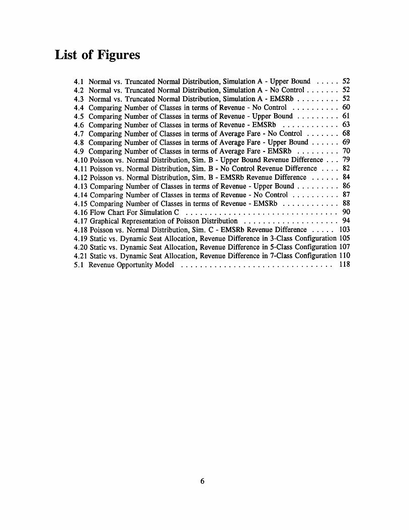
List of Figures

4.1 Normal vs.4.2 Normal vs.4.3 Normal vs.4.4 Comparing4.5 Comparing4.6 Comparing4.7 Comparing4.8 Comparing4.9 Comparing4.10 Poisson vs.4.11 Poisson vs.4.12 Poisson vs.4.13 Comparing4.14 Comparing4.15 Comparing

TruncatTruncatTruncatNumberNumberNumberNumberNumberNumberNormal

Normal Distribution, Simulation A - Upper Bound .....Normal Distribution, Simulation A - No Control .......Normal Distribution, Simulation A - EMSRb .........

of Classesof Classesof Classesof Classes:of Classesof Classes:Distributio

Normal DistributioNormal DistributioNumber of ClassesNumber of Classes

in terms ofin terms ofin terms of

Revenue - No Control .......Revenue - Upper Bound ......Revenue - EMSRb .........

in terms of Average Fare - No Control .......in terms of Average Fare - Upper Bound ......in terms of Average Fare - EMSRb .........n, Sim. B - Upper Bound Revenue Difference ...n, Sim. B - No Control Revenue Difference ....n, Sim. B - EMSRb Revenue Difference ......in terms of Revenue - Upper Bound .........in terms of Revenue - No Control ..........

Number of Classes in terms of Revenue - EMSRb ............4.16 Flow Chart For Simulation C .................................4.17 Graphical Representation of Poisson Distribution ....................4.18 Poisson vs. Normal Distribution, Sim. C - EMSRb Revenue Difference .....4.19 Static vs. Dynamic Seat Allocation, Revenue Difference in 3-Class Configuration4.20 Static vs. Dynamic Seat Allocation, Revenue Difference in 5-Class Configuration4.21 Static vs. Dynamic Seat Allocation, Revenue Difference in 7-Class Configuration5.1 Revenue Opportunity Model .................................

6061636869707982848687889094

103105107110118

ed

ed

ed

Chapter 1 Introduction

1.1 What is Yield Management ?

Anyone who has flown, especially in the past 5 to 10 years, thinks they know the

airline industry. One can almost be guaranteed that a heated conversation will arise

whenever the topic of discount air fares is mentioned. The majority of the travelling

public has, at some point, experienced some form of rejection from an airline reservation

agent or his/her own travel agent when making a particular request. Comments seem to

revolve around some kind of false advertising, and anyone in attendance working in the

airline industry will almost certainly be labelled as the one who helped to "squeeze" the

last penny out of the traveller. At least that is the author's personal experience.

Do these people truly understand the industry and more importantly, do they

understand the concept of Yield Management in the airline environment? Before we can

understand what yield management is, we must understand the marketing strategies of

an airline. The marketing department at any airline cannot be expected to meet the exact

requirements of all customers, as each customer is to a degree unique in his/her

requirements. It is therefore impossible for airlines to orient their product, pricing,

distribution and promotional policies to meet every customer's needs exactly. Marketing

is in fact a process of compromise whereby airlines seek to group together customers

whose needs are broadly similar. The process is known as Market Segmentation. A

market segment can be defines as follows :

"A group of customers who have sufficient in common to form a suitable basisfor a product, price, distribution, and promotion combination."'

Price differentiation is a very effective way to segment the air travel market, and in turn,

passengers. Most airlines practice seat inventory control to limit the number of seats that may

be sold at each of the fare products offered. In most airline reservations systems, limits are

placed on the number of seats available in each fare or booking class, each of which can contain

several fare products.2 The most common method for an airline to segment its passengers is

by offering multiple fare products; for the same seat in the coach cabin, you can pay 3, 4, 5 or

even up to ten different prices for the same service. Which price you are going to pay depends

on you abilities to meet different restrictions. By applying a number of different restrictions,

such as advance purchase requirements, penalties on changing/cancelling tickets, non-refundable

tickets, minimum and maximum stay requirements, an airline can effectively offer the same

service to a number of different types of passengers.

Seat Inventory Control/Management is the process of balancing the seats sold at each of

the fare levels offered so as to maximize total passenger revenues on a flight by flight basis,

within a given price structure. Seat inventory control and pricing are two distinct strategies that

together comprise airline yield management.

The term "Yield Management" is somewhat a misleading since revenue rather than yield

should be maximized. A more appropriate name may be passenger revenue management or

simply seat inventory control3 , since pricing policies are dictated by the behavior of other

airlines and the industry as a whole.

1.2 Benefits of Yield Management

Yield/Revenue Management is one of the three primary marketing functions of an airline.

Scheduling determines the supply of service offered -- with flights to and from different

origins/destinations and at different departure/arrival times; Pricing determines the number and

type of fare products offered and the price and restrictions of each; Yield Management

determines how much of each product (fare class for each origin/destination) to sell.

Yield Management does not generate demand, but it can stimulate it. Revenue or

profitability is theoretically increased by limiting seats to various passenger types in order to

preserve space for higher revenue, more profitable passengers. The scheduling and pricing

structure generate demand, while yield management accepts, rejects, and redirects demand.4

The potential benefits of filling seats with full-fare passengers that the airlines otherwise

might not carry due to too many low-fare passengers on board can be important to an airline's

profitability. One of the major U.S. carriers estimated that by carrying only one extra full-fare

passenger per flight it can generate about 50 million dollars of additional revenue per year.'

Therefore, the benefits of selling a seat to a low-fare passenger early in the booking process

must be weighed against the possibility of displacing a potential higher-fare passenger at a later

period. Effective yield management practice can be the single most important factor in

distinguishing between success or failure of an airline and spell the difference between

profitability and loss for a particular flight.

1.3 Objective of the Thesis

Yield Management through Seat Inventory Control plays an important role in terms of

the profitability of an airline, because if it is used properly, the airline can better utilize its

highly "perishable" assets (seats on a scheduled flight). The objective of Yield Management is

to maximize revenue; however, the real revenue impacts of a yield management system have not

be studied in any depth. Operations in airline industry are influenced by many external factors.

Therefore, any positive revenue impacts can be a combination of yield management and the

effects of these other outside factors. Hence, positive revenue impacts do not necessarily mean

that a given yield management system is working properly. The first step towards the study of

revenue impacts of airline yield management is to isolate the external factors. Airline

yield/revenue management performance plays an important role in convincing top executives that

the development of a sophisticated Seat Inventory Control system is worth the investment, since

the investment in any seat inventory control system generally requires substantial amounts of

both capital (computer hardware) and labor (programming, daily operations).

One of the primary objectives of this thesis is to remove most of the external factors

which influence airline operations in order to better understand the true revenue impacts of a seat

inventory control system. It is important to mention that due to the complexity of the revenue

impact measurement problem, our analysis will look only at the single flight leg case. Using

information gained from the single leg flight case, it might ultimately be possible to extrapolate

and apply our results to the much more complicated problem of the hub-and-spoke system.

1.4 Structure of Thesis

The remainder of this thesis is divided into four chapters. Chapter 2 contains a literature

review. In order to keep the research manageable, the scope of the thesis has been limited to

the single leg case, and the pricing portion of airline yield management is purposely left out,

under the assumption that airlines are more or less forced into setting their fare levels due to

competition from other carriers. Only a very limited number of studies have been done on

measuring the effectiveness of revenue management and revenue impacts of seat inventory

control methods, as described in Chapter 2.

Chapter 3 discusses the seat inventory control methodologies and different simulation

scenarios use in this study. There are a total of four inventory control "methods" used in the

research, they include two variations of the Expected Marginal Seat Revenue model, Upper

Bound and No Control analysis. In addition to the four seat inventory control methods, we will

also use a wide variety of different scenarios during the study to analysis the revenue impacts

of airline yield management systems. Some of the variables we use are, different number of

booking classes, Static versus Dynamic seat allocation, Single versus Multiple demand periods,

multiple capacity constraints and different assumptions on the demand distribution pattern.

Chapter 4 describes the three simulations used in this research, and presents a detailed

discussion for each of the simulations. The first simulation is performed using the @RISK

software -- it is a single period demand, single optimization booking simulation. The second

simulation is a multiple period demand, single optimization booking simulation and the third is

a multiple period demand and multiple optimization booking simulation. Both the second and

third simulation use a simulation program developed by the author. Analysis of the results from

the three simulation programs are also presented in this chapter.

Chapter 5 provides an overall conclusion based on the analysis of Chapter 4. We also

apply the results from one of the simulations in Chapter 4 to the Revenue Opportunity Model

developed by American Airlines Decision Technologies4 . The details of this model which

measures the revenue potential achieved through seat inventory control, will also be discussed

in Chapter 5.

1. Stephen Shaw, "Airline Marketing & Management", Third Edition.Pitman Publishing, London, England 1990.

2. Peter P. Belobaba, "Airline Travel Demand and Airline SeatInventory Management", Flight Transportation Laboratory,Massachusetts Institute of Technology, Cambridge, Massachusetts1987.

3. Yield Management, Revenue Management and Seat Inventory Controlare three terms that historically been used interchangeably.

4. AADT (American Airlines Decision Technologies), "YieldManagement for Airlines", 1989.

5. Peter P. Belobaba, "Airline Yield Management. An Overview ofSeat Inventory Control", Transportation Science, Vol. 21 Number 2,May 1987.

Chapter 2

Literature Review

2.1 Introduction

In this chapter we take a look at different studies that have investigated Yield

Management practice in the airline industry. The first section of this chapter gives an

overview of studies on yield management from the perspectives of the airlines as well

as the passengers. In the second section we review the literature on the methodologies

for seat allocation and setting booking limits. In the final section, we review the limited

literature on evaluating yield management systems performance, which includes both in-

situ and theoretical testing.

2.2 Looking at Yield Management

"American Airlines' yield management controllers are responsible for 38 million

seats at a time."

To most people, yield management/seat inventory control is something that the

airlines use to limit the number of the discount seats being sold. More specifically, seat

inventory control/yield management is the practice of balancing the number of discount

and full-fare reservations accepted for a flight so as to maximize total passenger revenue

and/or load factors. Load factors can increase when more seats are made available at

discount fares. However, selling too many seats at a discount fares level can cause yield

(per passenger revenues) to go down, and it can also lead to lower total revenues. In

order to prevent such revenue dilution, effective yield management is required which in

its truest sense includes both pricing and seat inventory control2 .

Pricing is usually determined by the pressure of competition from other airlines

such that virtually all airlines offer the same published fares in the large majority of

markets. Seat inventory control enables the airline to influence yields and total revenue

on a flight by flight basis with "predetermined" fare levels.

While airline marketing executives are pressured into setting fare levels by free

market competition, revenue control staffs constantly monitor and adjust the number of

seats offered to each fare level, in order to achieve the most profitable (maximum

revenue) mix from the available passenger demand. "Just as the sum of many small,

well trained, buy/sell decisions by security traders can produce large profits for their

brokerage houses, so can these small adjustments in seat allocations have significant

impact on carriers' profitability."I

In its 1987 annual report, American Airlines described the function of yield

management as "selling the right seats to the right customers at the right prices...". A

more detailed description of yield management, as it applies to airlines, is the control of

and management of the reservations inventory in a way that increases company

profitability, given the current flight schedule and fare levels. Yield management has

played a major role in allowing American Airlines to compete in an environment of

significant price competition. The biggest benefit of yield management is the increase

in revenue for AA : It has estimated a cumulative benefit of over $1.4 billion between

1986 - 1990. A secondary benefit of yield management in AA is the ability to sell its

technology to other industries, such as hotel chains and car rental companies3.

The airlines are apparently satisfied with the concept of yield management. How

about the travelling public -- are there any advantages for them? In a presentation by

Robert Cross of Aeronomics Incorporated4 , some of the benefits for the passengers due

to the use of yield management were described as follows. Due to the practice of

overbooking, a passenger will have a higher probability of getting booked on his/her

preferred flight/itinerary. Furthermore the concept of non-refundable tickets allocates

the costs of empty seats directly to those people imposing the costs, thus minimizing the

need to distribute the blame to others. However, in the world of multiple fare classes,

do full-fare passengers subsidize the discount passengers? The answer to this question

is no, as long as the revenue from low yield passengers exceeds the marginal cost5 of

carrying them, thus providing some contribution to overhead. Thus it is possible to

improve service (more frequency, larger equipment or last minute seat availability) which

full-fare passengers desire.

Airlines have realized that the price of a seat on a given flight is dictated by

demand not cost, the demand based pricing aspect of yield management makes it possible

for an airline to provide passengers with a level of service which would not be possible

otherwise. There might not be one single fare that the airlines can charge/offer on a

flight which will cover the costs of the operation. By practicing yield management and

offering multiple fare classes, an airline can generate enough revenues not only to cover

its costs it can also improve its future level of services.

It is the yield management system's job to balance the availability of seats among

the full-fare and various discount passengers so that the needs of each class of passengers

are met. Discount passengers want the lowest possible fare. They also desire the same

flights as the full-fare passengers, but they are rather flexible in terms of their time frame

of travel depending on the discount offered. Full-fare passengers want last-minute seat

availability on peak flights, and they are willing to pay a substantial premium over the

average price to assure the availability.

The yield management system must constantly monitor the changing relationship

between supply and demand of seats, and, in turn, adjust the discount availability to

assure last-minute seat availability for the full-fare passengers. By the same token,

discount seats must be made available in price elastic markets. Therefore, it provides

incentives for discount travellers to book on low-demand flights and save seats on peak

demand flights for full-fare passengers. Lastly, an effective yield management system

must understand the needs of the marketplace, offer seats according to market demands.

Since, "the ultimate dictator of the price mechanisms is the consumer....

2.3 Setting Booking Limits

Given the argument that Yield Management can be beneficial to both the airlines

and the passengers, the first component of yield management which interests us is how

booking limits are set. Therefore, we now examine some of the literature on this topic.

As early as 1972, Kenneth Littlewood of BOAC published a formula to optimize

the mix of early-booking, low-fare passengers and late-booking, high-fare passengers.

The formula is rather simple and intuitive, it recommends that low-fare bookings be

accepted as long as,

r> P*R

where R and r are, respectively, the average high-fare and low-fare revenue on a flight,

and P is the probability that the high-fare demand exceeds the number of seats set aside

for high-fare passengers.

Helmut Richter7 of Lufthansa presented a related approach to determine optimal

seat allotments by fare type using the differential revenue method. The method looks at

what will happen to the expected total revenue of the flight if one additional seat is

offered to the low-fare clientele, i.e. if the low-fare allotment is increased by one. And

the (expected) revenue differential DR due to one additional low-fare seat offered is equal

to,

DR = additional LF revenue minus HF revenue lost

and the optimal low-fare passenger allocation is,

ALO = C-H ( ARPL)ARPH

where H(x) is the high-fare demand value which is exceeded with a risk probability of

x, C is the capacity of the aircraft, ARPL and ARPH are the average revenue per

passenger (low-fare and high-fare respectively). The result is conceptually equivalent to

Littlewood's formula.

The application of the "marginal seat" principal described above succeeds in

explicitly incorporating probabilistic demand into the seat inventory revenue

maximization problem. However, the biggest shortcoming of these approaches relate to

their inability to deal in a practical way with setting static limits for multiple nested' fare

classes and to incorporate probabilistic demand at the same time. Belobaba in his Ph.D.

dissertation9, proposed that in order to overcome these shortcomings a different model

should be used. He proposed the Expected Marginal Seat Revenue (EMSR) model to set

optimal protection levels between any two fare classes and then to nest these protection

levels heuristically. The EMSR approach is used in this simulation study, and is

described in more detail in Chapter 3. The optimal solution for nested booking limits

on a single flight leg was proposed by Curry", Wollmer", and Brumelle and

McGill". These optimal nested booking limits can generate marginally higher expected

flight revenue in a static demand scenario, but these revenue differences become

negligible when the airline re-optimizes the limits periodically before departure.

2.4 Seat Inventory Control Evaluation

As mentioned in an earlier section of this thesis, studies in the area of seat

inventory control evaluation are very limited. A few people from the industry have

developed with theoretical models, yet not one has been fully tested and implemented.

Therefore, only a limited amount of research in this area can be presented and it should

set a tone for the needs of latter parts of this thesis.

Cross" proposed looking at Yield vs. Load Factor (normalized by passenger trip

distance) and performing, a correlation analysis on yield vs, load factors by segmenting

individual flights; by day and by season. He concluded that yield and load factor should

have a positive correlation and that the steeper the slope, the better the fare mix

management process. He also presented a quantitative method for evaluating the

effectiveness of revenue management. The method first determines the unconstrained

forecast for each booking class. Then it compares the ultimate unconstrained forecast to

the actual bookings and evaluates a revenue gain (loss) due to the inventory control

process.

AADT uses what they call a Revenue Opportunity model to measure revenue

performances as the percent of revenue opportunity achieved by seat inventory control.

This process is performed first by estimating potential revenue on a flight-by-flight basis

(which American would have earned with no discount controls) and then compare this

revenue to the revenue which would have been earned with "perfect knowledge". The

difference between the minimum and maximum revenues is the total opportunity that was

available through discount controls. The amount of revenue opportunity achieved is

determined by the actual revenue earned from the flights minus the minimum revenue.

Performance is measured as the percentage of revenue opportunity earned divided by the

total opportunity. This method will be used in the later part of this thesis to evaluate the

performance of different inventory control methods in a simulated environment.

Both Belobaba' and Bohutinsky" performed real-time yield management system

performance evaluation experiments in cooperation with Western Airlines and Delta

Airlines respectively. Belobaba studied the performance of the Automated Booking Limit

System (ABLS) developed at Western Airlines by carefully selecting individual flights

for use in ABLS, and comparing revenues to a set of corresponding flights subjected to

the controllers' experience to set booking limits. The flights set with the ABLS

consistently exhibited higher revenues and load factors than the flights monitored by

controllers. Bohutinsky assessed the "sell-up"'" potential in an airline environment on

a real-time basis. First, she identified flights with potential for sell up and then closed

a number of classes prematurely on these selected flights, the same flights were used in

alternate weeks as the control group was subjected to regular seat inventory control

practices. The differences in bookings were then determined and a revenue impact

test 7 by class was performed between the two groups. She concluded that sell up does

not exist on all flights and that sell up appears to be more prevalent in the higher fare

classes.

2.5 Conclusions

Most of the studies reviewed in this chapter looked at yield management, setting

booking limits and revenue impacts as three distinct problems. The studies reviewed in

the first section stressed the importance of yield management in the airline industry and

the benefits to both the airlines and the travellers. The studies in the second section

provided a brief overview of the process of setting booking limits. The last section

looked at performance evaluation. None of these studies have taken any detailed look

at the revenue impacts due to different yield management practices. A single-leg booking

simulation may be able to provide some insight into the relationship between revenue and

seat inventory control methods, and in a more general sense, it might also prove or

disprove the need for yield management by airlines.

A detailed study of the simulation outputs should provide valuable information to

any discussion on revenue impacts of yield management systems. We will study these

impacts using different seat inventory methods and different assumptions of demand, fare

class structure, fare ratios and combinations of some or all of the above items.

1. Samuel Fuchs, "Managing the Seat Auction", Airline BusinessJuly, 1987 pp 40-44.

2.Peter P. Belobaba, "Airline Yield Management. An Overview ofSeat Inventory Control", Transportation Science, Vol. 21 Number 2,May 1987.

3. Barry C. Smith, et al., "Yield Management at American Airlines",American Airlines Decision Technologies, 1990.

22

4. Robert G. Cross, "The Passenger's Case for Yield Management",Presentation at the second International Airline Yield ManagementConference.

5. Marginal cost is the most popular way to describe an airline'scost situation, due to the complexity of the cost structure of anairline. Marginal cost in its simplest form usually referred to asthe extra meal, extra can of soda, etc., attributed to anadditional passenger given that any other services are alreadyexisting.

6. K. Littlewood, "Forecasting and Control of Passenger Bookings",AGIFORS Symposium 1972.

7.Helmut Richter, Lufthansa, "The Differential Revenue Methods todetermine Optimal Seat Allotments by Fare Type", AGIFORS SymposiumXXII.

8. Peter P. Belobaba, "Airline Travel Demand and Airline SeatInventory Management", pp 107-108. MIT Flight TransportationLaboratory Report R87-7, 1987.

9. See Belobaba 1987.

10. R. E. Curry, "Optimal Seat Allocation with Fare Classes Nestedon Segments and Legs", Tech. Notes 88-1, Aeronomics Incorporated,Fayetteville, Ga., 1988.

11. R. D. Wollmer, "An Airline Seat Management Model for a SingleLeg Route When Lower Fare Classes Book First", ORSA/TIMSConference, Denver, Colo., 1988.

12. S. L. Brumelle and J. J. McGill, "Airline Seat Allocation withMultiple Nested Fare Classes", ORSA/TIMS Conference, Denver, Colo.,1988.

13. Robert G. Cross, "Assuring and Measuring the Success of RevenueManagement Programs", presented at the 3rd International AirlineYield Management Conference, Dec 3-4, 1990.

14. American Airlines Decision Technologies (AADT), "YieldManagement at American Airlines - Monitoring and Performance".

15. Catherine H. Bohutinsky, "The Sell Up Potential of AirlineDemand.", MIT Flight Transportation Laboratory Report R90-4, 1990.

16. Sell Up -- In the context of this thesis, if a passenger iswilling to Sell Up, this means that the passenger will pay more fora seat on a given flight (book in a higher fare class).

17. Revenue Impact Test -- See Belobaba 1987, pp 186-202 andBohutinsky 1990, pp 65-70.

Chapter 3

Methodologies / Scenarios

3.1 Setting Booking Limits

The main objective of seat inventory control is to limit the number of seats sold

at less than the full coach fare. This concept is based on the protection of seats for high-

fare passengers, and allows only those seats that would ultimately remain empty available

to discount passengers.

In a nested reservation system, like the one in our simulation, seat inventory

control must therefore be directed toward finding the protection level for higher fare

classes which can then be converted into booking limits for the lower fare classes. Each

protection level is the minimum number of seats that should be retained for a particular

fare class (and available to all higher fare classes). Each booking limit is the maximum

number of seats that may be sold to a fare class (including all lower fare classes with

their own, smaller, booking limits). The booking limit on the highest fare class is thus

the total capacity (or remaining capacity) of the shared cabin. The protection level for

24

the highest fare class is the difference between its booking limit and the booking limit of

the next class.1

In our simulation, we tested two versions of the EMSR control methodologies

developed by Belobaba' to calculate the booking limits for each class, which we will

refer to as EMSRa and EMSRb. In addition to these control methodologies, we also

used what we call Upper Bound and No Control methodologies to control the booking

procedures, and the following sections provide a detailed discussion of each of the four

methods.

3.1.1 Expected Marginal Seat Revenue Model - EMSRa

"EMSRa" refers to the basic Expected Marginal Seat Revenue model developed

by Belobaba in his PhD dissertation.' The expected marginal seat revenue of the Sith

seat in fare class i, EMSRi(Si), is simply the average fare level in that class multiplied

by the probability of selling Si or more seats:

EMSR i (S S2 ) =f ipi (Si )

The optimal values of S, and S2 in the case of two distinct fare class inventories

must satisfy:

EMSR, (S*) =EMSR2 (S2)

These optimal values of S, and S2 will depend on the parameters of the probability

densities of expected demand for each fare class, the relative fares or revenue levels, and

the total capacity available.

In the nested fare class case, the assumption of independent fare demand densities

can still be used, and given the historical density of requests for a fare class i and, in

turn, the expected bookings as a factor of Si, the revenue from Si seats available in class

i is:

~(= f *i (Si)

where f; is the net revenue or average fare calculated from the expected number of

passengers booked in class i, b;(S).

EMSR is defined to be the expected marginal seat revenue of class i when the

number of seat available to that class is increased by one. To illustrate this concept, we

consider a single-leg flight for which bookings will be accepted in two nested fare

classes, 1, and 2, having average fare levels fi and f2, respectively, f, > f2. In order to

maximize total expected flight revenues, the reservation process should give priority to

class 1 passengers. Class 1 will have the total available capacity of the shared cabin

capacity, C, as its booking limit, BL 1. The seats protected from class 2 and available

exclusively to class 1 will be denoted S12.

The optimal protection level S for class 1 is the largest integer value of S12 that

satisfies the following condition:

EMSR (S21) k f 2

The expected marginal seat revenue of the last seat in class 1 is set equal to the average

fare level of class 2 to find the optimal protection level for class 1.

The revenue-maximizing protection level for class 1 is determined in the EMSRa

model by finding the value of S12 which satisfies:

EMSRI (S ) =f 1 *N(S2) =f2

This optimal protection level is not a function of the lower fare class demand density in

the static case where nested classes are involved. It is a function of the ratio of f2 to fi

and of the parameters of the high fare demand density assumed from historical data.

Extension of the EMSRa model to more than two fare classes on a single flight

leg simply requires more comparisons of expected marginal revenues be made among the

relevant classes. In general, if we have k fare classes on a flight leg, Belobaba stated

that each of the optimal values of S' must satisfy the following equation:

EMSR1 (Sj ) = f4, i<j, j=1, . .. k

and the nested booking limits are

BLj = C-E S1i<j

Readers interested in more details of the EMSR model can refer to Belobaba's

dissertation pages 101-157.

3.1.2 Expected Marginal Seat Revenue Model - EMSRb

In contrast to the EMSRa model in which the seat protection level S' is found

between each pair of classes i<j and then nested heuristically, the EMSRb approach

finds the total protection level for the aggregate of all classes i<j 2. Some of the

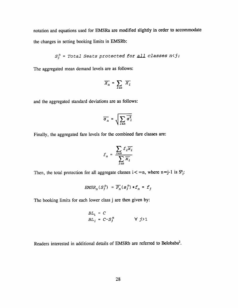
notation and equations used for EMSRa are modified slightly in order to accommodate

the changes in setting booking limits in EMSRb:

Sj = Total Seats protected for .a.U classes n<j;

The aggregated mean demand levels are as follows:

isn

and the aggregated standard deviations are as follows:

Jnn

Finally, the aggregated fare levels for the combined fare classes are:

issn

Then, the total protection for all aggregate classes i< =n, where n=j-1 is S"j:

EMSRn (Sjn) = P (sip) *fn = fj

The booking limits for each lower class j are then given by:

BL 1 = C

BL1 = C-Sn V j>1

Readers interested in additional details of EMSRb are referred to Belobaba2.

3.1.3 Upper Bound

The modelling of Upper Bound is slightly different from the EMSR control

methods. The concept of "Upper Bound" has been described by Smith et al. of

American Airlines3 and presented in greater detail by Williamson4. First, we generate

total demands for each fare class for all revision periods. No booking limits are set for

any given class and the booking process is not performed until all demands are

generated. Bookings are then made for each class in a top-down fashion, from the

highest fare class to the lowest. The booking process for the second highest class will

not begin until all of the demand from the highest class has been satisfied, since no

booking limits are set. As long as the remaining capacity is greater than zero, no

demand is spilled. By following this algorithm, we generate an estimate of maximum

total revenue under "perfect information", with no uncertainties in the forecast.

The results from the Upper Bound analysis are used as the "ceiling" or "best

case" in the Revenue Opportunity model in Chapter 5. The combination of the results

from the upper bound analysis and the No Control case will provide a useful tool to

evaluate the effectiveness of revenue control practices within this range of revenue

outcomes.

3.1.4 No Control

Before we can start talking about "No Control", we must be sure that we know

exactly what "No Control" means. We must distinguish the difference between No

Control and Lower Bound. It is obvious that no control means no inventory control was

done but it does not necessary generate the lowest possible revenues, which is what

"Lower Bound" means. "No Control" simply follows a "first come first served" policy,

much like the Upper Bound case with no preset booking limits. As long as the remaining

capacity is greater than zero, the demand will be satisfied.

The simulation of "No Control" is more or less similar to that of the EMSR

control methods except that it does not have a set of pre-determined booking limits. The

booking process for the "No Control" analysis is essentially the same as for the EMSR

models. The outputs of the "No Control" analysis are the revenue and booking results

with no inventory control efforts. The theory will become more transparent when the

results of the simulation are discussed in the next chapter.

3.2 Scenario Analysis

The focus of this thesis is to try and answer some of the most commonly asked

questions about the revenue impacts of airline yield management. We look at the

difference in revenue contributions by having different capacity constraints, different

number of fare classes, "static" versus "dynamic" seat allocation methods, different

assumptions on demand distribution patterns, and our confidence in the demand

forecasting. These variables will become more obvious and easy to understand after the

discussions presented in the following sections.

3.2.1 Base Demand Scenario

The basic demand profile is based on historical booking information obtained from

a major U.S. carrier for its domestic services in the summer of 1991. This demand

profile is based on a seven-booking-class configuration with ten revision periods used to

record the demand data. These revision points are predetermined dates prior to departure

(DPD) to reflect the booking pattern along the overall booking process.

This is an aggregate demand arrival pattern, and it has been edited in order for

it to be useful in our simulation. One important note about these data : the absolute

values of demand do not have much importance in terms of the final results, as we can

change the final demand to our desired level rather easily. What we are truly after is the

percentage of final demand that arrives over time, in other words, Incremental Demand.

In our simulation, the first check (revision) point is fifty-six days prior to departure and

the last check point is taken at the date of departure. A spreadsheet program was created

using Lotus 1-2-3 based on the percentage of final demand arriving over time. We

simply input the "desired" total demand for the flight -- individual demands for each and

every class at each revision point is then calculated. Table 3.1 is an example of the

percentage of final bookings in each fare class at different revision points. If we use an

expected total demand of 200, Table 3.1 also presents the incremental demands for each

fare class at each individual revision point.

The individual class fare for our simulation is also calculated from the above

spreadsheet program. Based on current ratios between different fare classes in U.S.

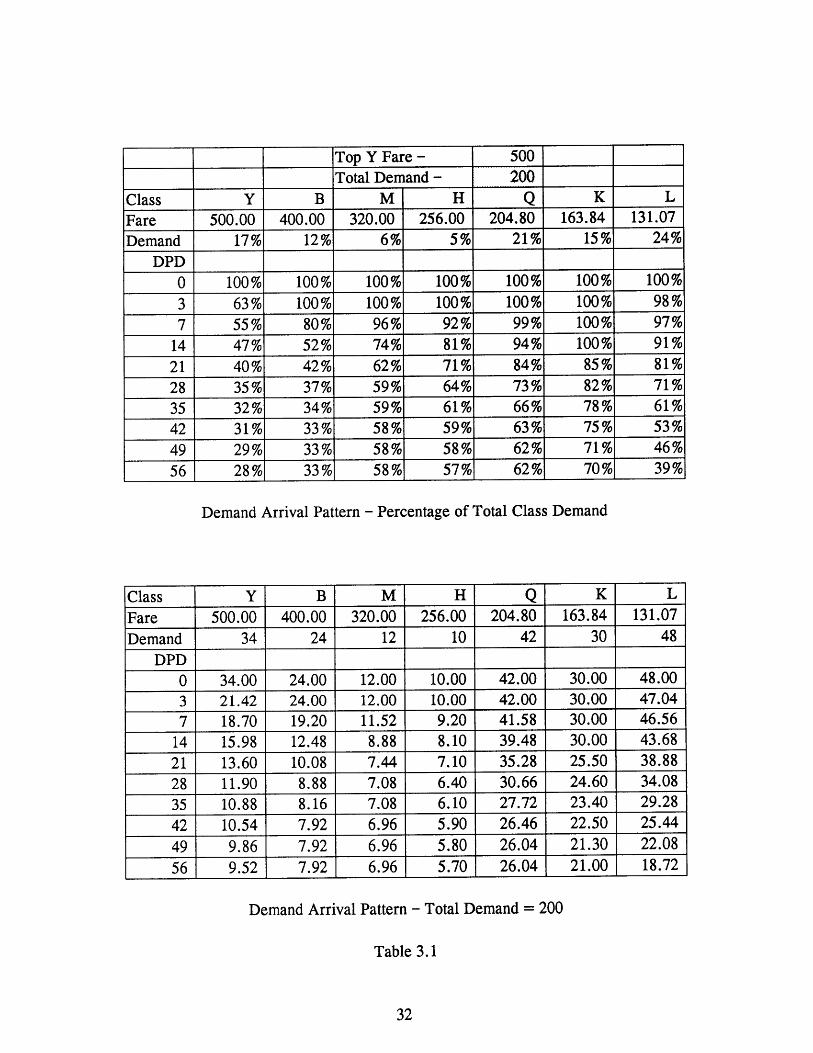
Top Y Fare - 500

Total Demand - 200

Class Y B M H Q K LFare 500.00 400.00 320.00 256.00 204.80 163.84 131.07Demand 17% 12% 6% 5% 21% 15% 24%

DPD0 100% 100% 100% 100% 100% 100% 100%3 63% 100% 100% 100% 100% 100% 98%7 55% 80% 96% 92% 99% 100% 97%

14 47% 52% 74% 81% 94% 100% 91%21 40% 42% 62% 71% 84% 85% 81%28 35% 37% 59% 64% 73% 82% 71%35 32% 34% 59% 61% 66% 78% 61%42 31% 33% 58% 59% 63% 75% 53%49 29% 33% 58% 58% 62% 71% 46%56 28% 33% 58% 57% 62% 70% 39%

Demand Arrival Pattern - Percentage of Total Class Demand

Class Y B M H Q K LFare 500.00 400.00 320.00 256.00 204.80 163.84 131.07Demand 34 24 12 10 42 30 48

DPD0 34.00 24.00 12.00 10.00 42.00 30.00 48.003 21.42 24.00 12.00 10.00 42.00 30.00 47.047 18.70 19.20 11.52 9.20 41.58 30.00 46.56

14 15.98 12.48 8.88 8.10 39.48 30.00 43.6821 13.60 10.08 7.44 7.10 35.28 25.50 38.8828 11.90 8.88 7.08 6.40 30.66 24.60 34.0835 10.88 8.16 7.08 6.10 27.72 23.40 29.2842 10.54 7.92 6.96 5.90 26.46 22.50 25.44

49 9.86 7.92 6.96 5.80 26.04 21.30 22.0856 9.52 7.92 6.96 5.70 26.04 21.00 18.72

Demand Arrival Pattern - Total Demand = 200

Table 3.1

airline markets, we decided to use 0.80 or 80% as our constant fare ratio between any

two adjacent fare classes. Since the absolute value of the fare is not important to us as

long as the ratio of the fare is within a reasonable range, we arbitrarily chose $500.00

as the fare for the highest fare class. Based on the 0.80 fare factor, the fare for class

number two is $400.00 and the fare for the third fare class is $320.00 and so on. Table

3.1 presents all of the individual class fares in the demand table.

3.2.2 Varying the Number of Booking Classes

The first parameter we vary is number of fare classes. We examined three

different configurations. We use 3, 5, and 7 booking class configurations to study the

revenue impacts of airline yield management. The use of a 7-class configuration is

natural, since the original demand data are in this format, thus it makes sense to include

this as one of the three variations. Moreover, the most common number of booking class

configuration used by the U.S. airlines is either a 7 or 8 class format. In the nested fare

class environment, the EMSR model yields the optimal booking limits in a 2 class

configuration, and for any configuration over 2, the booking limits are heuristic in nature

but very close to optimal.

What criteria did we consider when we are looking at the revenue impacts due

to different class configurations, and how did we arrive at the 3, 5, 7-class

configurations? Since the original demand profile is in the 7-class configuration, it seems

reasonable to include the 7-class configuration as one of the three choices. In addition,

a majority of the U.S. domestic airlines use a typical 7-class nested configuration.

However, there are many international carriers that still use a 3-class configuration to

control their passenger mixes, this is mainly due to the lack of sophisticated reservation

and revenue management systems. Therefore, the three classes configuration is another

obvious choice and the 5-class is simply the 'middle-of-the-road' choice.

When we go from 7 to 5 classes, we will group four of the existing classes

together to form two "aggregate" ones. We can not simply drop two classes to form 5

new ones, because important booking information would lost. We propose to group

classes together based on the similarities in restrictions applying to them, thus Q and K

are the first two classes to be grouped to form a new class Q/K -- as they both have

similar restrictions such as 14 days advance purchase and a penalty for cancelling. Class

M and H are combined to form the next grouped class, M/H also based on the

philosophy of similar restrictions. Class Y, B, and L are untouched at this level because

they represent the two extreme ends of booking restrictions. We are trying to have three

rather distinct groups from the five remaining fare classes to represent low, medium, and

heavy restriction levels. Classes Y and B represent the least restricted group, classes

M/H, Q/K belong to the medium restricted group and L is the deeply discounted, with

heavy restrictions imposed.

Once we have completed the necessary analysis with five booking classes, the

next step is to reduce the number of classes further to a 3-class configuration. In order

to retain the 3 distinct groups of fare classes in terms of ticket restrictions, we will group

class B with M/H and L with Q/K, and allow Y to remain alone. Y represents the

unrestricted, full coach fare tickets, B/M/H the medium restriction tickets, typically with

a 3 or 7-day advance purchase requirement and some penalties on change of tickets and

finally, Q/K/L represents the heaviest discounted ticket with a minimum of 14-day

advance purchase requirement and usually non-refundable or with substantial penalty.

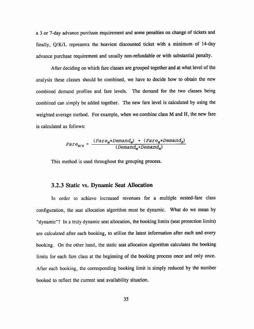
After deciding on which fare classes are grouped together and at what level of the

analysis these classes should be combined, we have to decide how to obtain the new

combined demand profiles and fare levels. The demand for the two classes being

combined can simply be added together. The new fare level is calculated by using the

weighted average method. For example, when we combine class M and H, the new fare

is calculated as follows:

= (Far e,*Demand) + (Far eH*DemandH)Fare (DemandM+DemandH)

This method is used throughout the grouping process.

3.2.3 Static vs. Dynamic Seat Allocation

In order to achieve increased revenues for a multiple nested-fare class

configuration, the seat allocation algorithm must be dynamic. What do we mean by

"dynamic"? In a truly dynamic seat allocation, the booking limits (seat protection limits)

are calculated after each booking, to utilize the latest information after each and every

booking. On the other hand, the static seat allocation algorithm calculates the booking

limits for each fare class at the beginning of the booking process once and only once.

After each booking, the corresponding booking limit is simply reduced by the number

booked to reflect the current seat availability situation.

Today's airline reservation systems attack this problem with a non-static, though

not truly dynamic approach. They re-optimize booking limits at some predetermined

revision points based on historical information about the incremental demand and also

the booking restrictions. When the revision points are judiciously chosen, the

incremental demand becomes relatively small in each fare class, thus the outcome of

using this method should be very close to the optimal booking limit algorithm.

We will perform our simulation with both the static and semi-dynamic (revision

point) approaches. In the static case, booking limits are calculated at the beginning of

the booking process, based on total expected demand to come. Information about newly

booked reservations will not be utilized. However, in the revision point (semi-dynamic)

case, we are going to use ten revision points during the booking process with nine

separate optimization. At each revision point, in addition to expected demand to come

information, we will also utilize the latest booking information from the previous period

that is available to us. Since we have a total of ten revision points, the incremental

demand between any two revision points should be relatively small, therefore, the final

booking limits should be reasonably close to the optimal level.

3.2.4 Probability Distribution Pattern

The airline seat inventory management problem is probabilistic in nature because

of the existence of uncertainty with regard to the final number of requests that an airline

will receive on a future flight. The total demand for a particular flight not only

fluctuates by day of week and season of the year, there will also be stochastic variation

in demand around expected or historical values. This stochastic demand for a future

flight departure can be represented by a probability density function, and with past

experience, a Gaussian (Normal) distribution is generally assumed.

Based on past analysis, the assumption of using the Gaussian distribution for the

demand arrival pattern is a valid one, if we are talking about the total expected demand

over the whole booking process. When we start using the concept of dynamic seat

allocation with multiple revision/optimization points, the Gaussian distribution assumption

still remains valid over the entire booking process. However, for each individual

revision period, it is more appropriate to assume that the demand arrival pattern follows

a Poisson distribution within a small interval, rather than the Normal distribution. The

use of Poisson demand distribution in the simulation of a dynamic booking process is

introduced and described in detail by Williamson5. It is not our goal to prove or

disprove either of these two assumptions. We are simply trying to study the difference

in revenue estimates by using either of the two probability distribution assumptions.

3.2.5 The Accuracy of the Forecast

Once again, our demand information is obtained from a major U.S. carrier and

represents the domestic system-wide historical mean demand arrival pattern. We have

to devise a method to calculate the standard deviations within each individual demand

period, as well as for the total remaining demand from each checkpoint to departure.

Since the demand data are organized in ten revision periods, and we have assumed the

demand within each period will follow a Poisson distribution, we are going to assume

the individual standard deviation is equal to the square root of the corresponding mean

demand, or:

(=4Iv, s=V1x

This assumption is reasonable based on no other information available to us about the

actual standard deviations regarding the booking patterns and with the overall demand

distribution still assumed to follow the Gaussian distribution.

Although these demand data came from an actual airline's data base, and they

have been "cleaned" up for the purpose of our simulation. There is no guarantee,

however, on the accuracy of using historical data as a forecasting tool. What will

happen, then, to our overall revenue contributions if these historical demand are

significantly different from the future demand?

A rather simple way to address this problem in our study is to place a higher

degree of variation on each of the demand points. We can achieve this variation by

scaling our originally calculated standard deviation, or:

a=k*W, s=k*i/x

where k is any positive real number.

With the results of this section, we can study the revenue impacts when the

demand forecast is not certain and/or your confidence in the forecast is rather low.

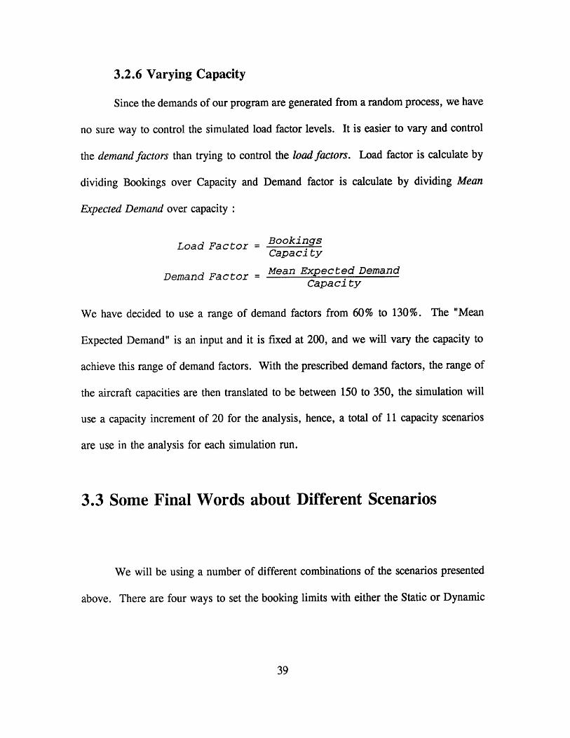
3.2.6 Varying Capacity

Since the demands of our program are generated from a random process, we have

no sure way to control the simulated load factor levels. It is easier to vary and control

the demand factors than trying to control the load factors. Load factor is calculate by

dividing Bookings over Capacity and Demand factor is calculate by dividing Mean

Expected Demand over capacity :

Load Factor = BookingsCapacity

Demand Factor = Mean Expected DemandCapaci ty

We have decided to use a range of demand factors from 60% to 130%. The "Mean

Expected Demand" is an input and it is fixed at 200, and we will vary the capacity to

achieve this range of demand factors. With the prescribed demand factors, the range of

the aircraft capacities are then translated to be between 150 to 350, the simulation will

use a capacity increment of 20 for the analysis, hence, a total of 11 capacity scenarios

are use in the analysis for each simulation run.

3.3 Some Final Words about Different Scenarios

We will be using a number of different combinations of the scenarios presented

above. There are four ways to set the booking limits with either the Static or Dynamic

approach, three different number-of-classes configurations, and multiple ways to calculate

the necessary standard deviation. Finally the coach cabin capacity will also be a varied.

As one can see, the number of simulation runs has to be increased dramatically

in order to accommodate all of the above combinations. With all the information

generated from our simulation, it is our hope to present a clear picture on the subject of

Revenue Impacts of Airline Yield Management in the next chapter.

1. Peter P. Belobaba, "Air Travel Demand and Airline Seat InventoryManagement", MIT Flight Transportation Laboratory R87-7, 1987.

2. Peter P. Belobaba, "Heuristic vs. Optimal Seat Allocation toNested Booking Classes", Working Paper, MIT Flight TransportationLaboratory forthcoming, Feb. 1992.

3. Barry C. smith et al., "Yield Management at American Airlines",American Airlines Decision Technologies, 1990.

4. Elizabeth L. Williamson, "Comparing of Network vs. Leg-BasedOptimization in Airline Origin-Destination Seat Inventory Control"ORSA/TIMS Joint Meeting, Anaheim, CA, Nov 1991.

5. Elizabeth L. Williamson, "Airline Network Seat Inventory Control: Methodologies and revenue Impacts.", MIT Ph.D. Dissertationforthcoming March 1992.

Chapter 4

Simulations

4.0 Overview of The Simulation

The airline industry is an extremely dynamic industry constantly affected by a

number of different external factors. The particular facet of the airline industry in which

we are interested is the practice of Yield Management (Revenue Management). Just as

any other part of airline operations, revenue management is constantly influenced by

externalities. Therefore, in order to perform a meaningful analysis, we must develop an

effective way to separate these externalities from our topic of interest. A simple example

of how external factors might mask the impacts of a new revenue management system

will illustrate the need for isolation.

Airline X has been working on their first revenue management system -- RYAN

(Revenue and Yield Advantages Network) for quite some time, and they have completed

all of the necessary testing, and it is time to put the system in place and fully implement

it. After six months of implementation and regular use, the results look rather

encouraging. A significant increase in revenue has been observed compared to the same

periods last year (adjusted for the rate of inflation). In addition to the increased

revenues, the system wide load factors have also increased. However, before the

revenue manager approaches his supervisor with the good news, he realizes that about

the same time RYAN was put in use, a major increase in leisure passenger traffic was

experienced. The sudden increase in traffic was mainly due to a new and more

competitive marketing strategy employed by Airline X. Now the revenue manager is

faced with a tough problem. He wants to prove to upper management that the new

revenue management system works and that it has helped the company to increase its

revenue significantly over the same period a year ago. However, it is rather obvious that

the new marketing strategy also had its contribution to the revenue hike. He had no idea

of how to differentiate what portion of the benefit was due to RYAN and how much of

the benefit could be contributed to the new marketing ploy.

Although this is a simplified example, it is rather easy to recognize that when

dealing with all these externalities in the industry, the effects of any revenue management

strategy can easily be over shadowed by something else. Another fact that makes the

evaluation process even harder is that each individual flight departure is different from

the previous one -- like fingerprints, no two are identical. One set of inventory control

actions might work extremely well for a flight today, but it might spell disaster for the

next day.

Therefore, the concept of a simulation is worth studying. In a simulated

environment it is much easier to control the factors influencing the outcomes. Also, a

single departure can be examined over a number of scenarios with different aircraft

capacities and other parameters, in order to test the impacts of each new situation. This

is the primary motivation behind this thesis and in the following sections I will discuss

the simulation in a more detailed manner.

We will perform our analysis with three different simulations. The first

simulation is a single period demand, fixed seat allocation booking simulation using the

@RISK software package. The second simulation uses multiple demand periods, but

retains a fixed set of seat allocations, using computer code developed by the author. The

third is a multiple demand period and multiple optimization simulation using the program

similar to the one used in the second simulation. A detailed description and discussion

of these three simulations will be presented in the following sections along with their

results.

4.1 Simulation A - Single Demand Period, Single

Optimization

The first simulation we used is a simple single period demand, single optimization

simulation using a commercial software package named @RISK.

4.1.1 Description of the Simulation

This is the simplest of the three simulations we used during this study. It is a

basic single-leg, single period demand, single optimization simulation. The demand for

a given flight scenario under investigation arrives in the form of "Final" or "Total"

demand for that flight in a multiple nested fare class configuration. The booking limits

for this particular flight are calculated for the total demand by fare class by using one of

the seat inventory methods discussed in Chapter 3.

The booking limits, along with all other necessary information such as nested

protection levels, fare information, are then used in the simulation performed with the

@RISK software. A number of different combinations of demand distributions, number

of booking classes, capacity constraints, and variations of calculated standard deviations

are then used as variables to study the revenue impacts of an airline yield management

system under different conditions.

The mean demand for each fare class and its corresponding standard deviation

were entered into the spreadsheet with a specified probability distribution for generating

future demand. The spreadsheet was set up in such a way that three sets of standard

deviations are used at the same time with the same mean demand assumption, hence,

three sets of output are being generated during each simulation. The fare information

was entered into the spreadsheet also -- these data were used at the end of the simulation

to calculate the total revenue results.

The booking limits are also required by the program. In the case of EMSRa and

EMSRb, their respective booking limits were first calculated from a separate algorithm

with the given demand and fare level. After the booking limits were calculated, they

were also entered into the spreadsheet. Since we ran three sets of standard deviations

at the same time, three sets of booking limits were needed as inputs.

Authorization Levels (AU) were computed from the capacity and booking limit

information in the spreadsheet itself. The authorization level for class i is the difference

between the authorization level of class i-I and the protection level for class i-1, and this

is true for all classes except the highest booking class. The AU for the highest fare class

is simply equal to the capacity or remaining capacity of the aircraft.

The next step after the protection levels have been calculated was to perform the

booking process itself with @RISK. Since this is only a single demand case, the booking

process is rather simple, a single decision based on the comparison of the generated

demand level and the authorization level in each booking class. The basic decision rule

is as follows

n

BK = min(DM1 , AU - BK)i+1

where BK; is the number of bookings for class i and DMj and AUj are the randomly

drawn demand and authorization level for class i respectively, and n is the total number

of booking classes. Thus, the number of bookings allowed for class i is equal to the

lesser of the demand for class i or the authorization level for class i minus the total

number of bookings have already made for all classes below i. This process becomes

much more obvious with a simple numerical example.

For the sake of discussion, let us assume we have seven different fare classes and

their demands, authorization levels (AU) and bookings are as shown in Table 4.1. The

booking process in the first simulation using @RISK follows a "Bottom Up" rule, which

simply means that the lowest class is booked first and then the next lowest one, until all

classes have been booked. For Class 7, by following the decision rules presented above,

no passengers are accepted in this particular case, since its AU is equal to zero. The

next class up is Class 6, it has a demand of 57 and an AU of 29, and nothing was

booked for class 7, therefore, we book as many as the AU allows us to, which is 29

reservations. Now it is Class 5's turn, it has a demand level of 42 with an AU of 71 and

the sum of all bookings from class 6 and 7 is 29, therefore, we will book the minimum

of (42, 71-29) which is 42. Once we have finished the booking process for class 2 to

7, we have to book for the highest class. Class 1 has the following characteristics

DM=44, AU= 150 and sum of all bookings below class 1 is equal to 110, therefore, by

following the same decision rule we allowed 40 out of the 44 requests drawn as demand

for class 1 to become actual reservations.

The above booking process is typical for the cases in which EMSR booking limits

are applied. However, for the "No Control" case, the booking process is basically

identical with the exception being the absence of booking limits for each individual

booking class. This modification to the booking process is necessary in order to reflect

the first come first served, no inventory control condition in the "No Control" case,

hence the name (Table 4.2).

In the case of "Upper Bound", we are trying to simulate the situation where

perfect information about future demand is assumed available to us and the maximum

amount of revenue will be achieved with the "known" demand profile. The booking

process is also modified in order to achieve this goal, a "Top-Down" booking process

is used rather than the "Bottom-Up" one that had been used so far. The "Top-Down"

booking process simply means that we are booking from the top, the highest fare class

is booked first and then down the hierarchy to the lowest one. By booking the highest

fare class first, we assure that the next available seat goes to the next highest yield

passenger, therefore generating the highest total revenue. The booking criteria are as

follows :

BK, = min (DM1 , Capacity)i-1

BK = min (DM1 , Capaci ty-j BK) n i>11

where BKi and DMi are the same as before. They represent the bookings and demand

for class i respectively, and n is the total number of booking classes. Based on the

perfect information assumption and using the above booking criteria, the final bookings

are guaranteed to yield the highest possible revenue for a fixed set of demand profiles.

Table 4.3 will help to illustrate the booking process and its results.

It is rather obvious from Table 4.3 that all of the demand is satisfied from the

highest class downward as long as the capacity or remaining capacity allows us to do so.

This portion (Upper Bound) of the analysis is extremely important to our overall study.

It provides us with a measuring stick to compare with other inventory control methods.

As one can see, with the same demand profile, the Upper Bound resulted in an additional

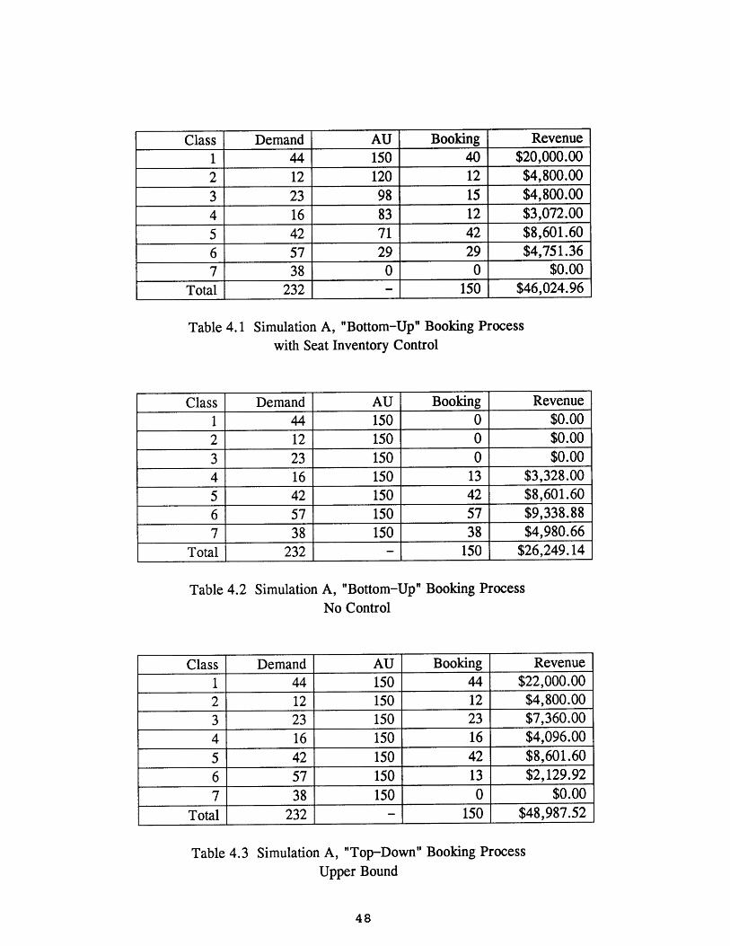
Class Demand AU Booking Revenue1 44 150 40 $20,000.002 12 120 12 $4,800.003 23 98 15 $4,800.004 16 83 12 $3,072.005 42 71 42 $8,601.60

6 57 29 29 $4,751.367 38 0 0 $0.00

Total 232 - 150 $46,024.96

Table 4.1 Simulation A, "Bottom-Up" Booking Processwith Seat Inventory Control

Class Demand AU Booking Revenue1 44 150 0 $0.002 12 150 0 $0.00

3 23 150 0 $0.004 16 150 13 $3,328.00

5 42 150 42 $8,601.60

6 57 150 57 $9,338.88

7 38 150 38 $4,980.66Total 232 - 150 $26,249.14

Table 4.2 Simulation A, "Bottom-Up" Booking ProcessNo Control

Class Demand AU Booking Revenue1 44 150 44 $22,000.002 12 150 12 $4,800.00

3 23 150 23 $7,360.004 16 150 16 $4,096.00

5 42 150 42 $8,601.60

6 57 150 13 $2,129.92

7 38 150 0 $0.00Total 232 - 150 $48,987.52

Table 4.3 Simulation A, "Top-Down" Booking ProcessUpper Bound

revenue of $2,962.56 which translated to 6.4% above the EMSRa model in this

deterministic analysis. In our simulation, demands are drawn randomly for fifty

iterations or "flight departures", so that we can compare expected revenues.

Now we know how the simulation is performed, but why are we doing it? The

primary reason for doing this analysis is to study the revenue impacts of an airline

revenue management system. To be more precise, we would like to look at the revenue

impacts under different booking scenarios. These different scenarios include different

demand distribution assumptions, number of booking class configurations and different

inventory control methods over a large number of different capacity levels. The

following section presents the results of the first simulation using @RISK and also

discussions of these results.

4.1.2 Results of Simulation A

First, we have to decide which demand distribution assumption is most

appropriate for the purpose of Simulation A. Since it is a single demand, single

optimization simulation, the Normal distribution comes to mind. Based on past studies

and general industry practices, the Normal distribution assumption for total demand in

each fare class is a valid one, and we will be using the Normal distribution in Simulation

A.

However, due to the properties of the Normal distribution and the possibility of

low mean demands in a fare class, it is possible to randomly draw a negative demand

value during the simulation process, but it is not possible to have a negative demand in

the real world. Therefore, we examined a variation of the Normal distribution in order

to eliminate the possibility of having a negative demand. The distribution we tested is

the Truncated Normal distribution. It is very similar to the Normal distribution but it

has maximum and minimum limits on the possible demand outcome. We used a

minimum of zero to eliminate the possibility of negative demand and a arbitrarily large

number of 750 for the maximum. With a total expected demand of 200 for all booking

classes used in the simulation, and demands generated at each individual class level in

each demand period, an upper bound of 750 is well beyond the three standard deviations

range of the mean demand for each class during any individual demand period, hence the

chance of drawing a demand over 750 is minuscule.

We know the Normal distribution is a valid assumption based on past experience,

and what kind of impacts will the Truncated Normal distribution have on revenue? To

answer this question, we performed the simulation with both the Normal and Truncated

Normal assumption and compared the revenue impacts. For ease of comparison, we only

performed the two simulations with a single 7-class configuration under different

scenarios using different capacity constraints. It is our belief that the 7-class

configuration alone is adequate for the purpose of comparing distribution assumptions.

In addition, the 7-class configuration in the coach class is the most widely used

configuration in the U.S. airline industry.

From the results of this analysis, we observed no significant differences in terms

of the revenue measures between the Normal and Truncated Normal distribution. This

result is consistent for the Upper Bound, No Control and the Expected Marginal Seat

Revenue model (EMSRb) for seat inventory control. This can be seen rather easily by

examining Figures 4.1 to 4.3.

The revenue differences between the two distribution assumptions are minimal.

The percentage difference in terms of total revenues between the two, ranges from -

0.14% to +0.30% when the Normal distribution is compared to the Truncated Normal

distribution in the case of Upper Bound. This difference is not significant enough for

us to make any judgement on which distribution should be chosen, and more importantly,

the randomly generated demands between the two distributions are also very close to

each other. No demand difference of greater than 0.20% was observed and all of the

mean simulated demands lie very close to the input expected demand level of 200. As

a matter of fact, the simulated mean demands range from 199.73 to 200.24 in all cases.

Therefore, the decision of which demand distribution should be used cannot be made

based on the results from our analysis. However, intuitively it makes more sense to use

the Truncated Normal distribution assumption, since we do not want to have any negative

demand values drawn during the simulation process.

With the total expected demand being 200, Table 4.4 shows the randomly

generated demands for all capacities under both demand distribution assumptions. Table

4.5 to 4.10 present a summary of the differences between the two distributions in both

absolute and percentage terms, under the Upper Bound, No Control and the EMSRb

inventory control scenario. These tables reinforce the arguments presented above that

the simulation results are inconclusive when trying to decide which distribution should

Normal vs. Truncated Normal Distribution7 Classes, Simulation A

50 -

45 -

40 L-

150 170 190 210

M Normal-Upper Bound

230 250 270 290 310 330 350

Capacity

T Normal-Upper Bound

Figure 4.1

Normal vs. Truncated Normal Distribution7 Classes, Simulation A

150 170 190 210 230 250 270 290 310 330 350

Capacity

Normal-No Control ii T Normal-No Control

Figure 4.2

53

'A40

35

30

25

Normal vs. Truncated Normal Distribution7 Classes, Simulation A

150 170 190 210 230 250 270 290 310 330 350

Capacity

iM Normal-EMSRb L3 T Normal-EMSRb

Figure 4.3

11-10

>

Capacity EMSRa EMSRbLevels Normal T.Normal Normal T.Normal

150 200.09 200.26 199.96 199.92170 200.10 200.01 199.88 200.00190 199.96 200.03 200.00 200.00210 200.26 200.32 199.92 199.80230 199.96 199.87 200.00 200.15250 200.08 199.84 199.99 199.98270 200.27 199.92 199.73 200.08290 200.00 200.05 200.10 200.01310 200.18 200.21 200.16 200.07330 199.90 200.14 200.24 200.17350 199.81 200.14 199.85 200.04

Capacity Upper Bound No ControlLevels Normal T.Normal Normal T.Normal

150 200.22 199.84 200.26 199.97170 199.85 199.91 200.43 200.08190 200.15 200.06 200.28 199.89210 200.19 200.24 200.07 199.95230 199.97 199.84 199.88 200.02250 199.91 199.97 200.00 200.26270 200.13 199.98 200.01 199.84290 200.10 199.97 199.97 200.01

310 199.94 199.90 200.04 200.02330 200.03 199.90 199.94 199.97350 199.96 200.05 200.02 199.99

Table 4.4 Simulation A - Generated Demand Table

55

Capacity Demand Booked Revenue Load Factor Spill Avg. Fare

150 0.38 0.00 140.42 0.00% 0.38 0.94

170 -0.06 0.03 -23.81 0.00% -0.09 -0.19190 0.09 0.10 42.90 0.00% -0.01 0.08210 -0.05 0.69 75.11 0.00% -0.74 -0.55230 0.12 0.00 9.79 0.00% 0.12 0.04250 -0.06 -0.06 13.85 0.00% 0.00 0.15270 0.15 0.15 32.39 0.00% 0.00 -0.04

290 0.13 0.13 11.09 0.00% 0.00 -0.12

310 0.05 0.05 48.59 0.00% 0.00 0.18330 0.13 0.13 31.54 0.00% 0.00 -0.01350 -0.09 -0.09 -74.86 0.00% 0.00 -0.25

Table 4.5 Simulation A - Upper Bound, Normal vs. Truncated NormalAbsolute Differences (Normal-Truncated Normal), 7 Classes

Capacity Demand Booked Revenue Load Factor Spill Avg. Fare150 0.19% 0.00% 0.30% 0.00% 0.76% 0.30%170 -0.03% 0.02% -0.05% 0.02% -0.30% -0.06%190 0.04% 0.05% 0.08% 0.05% -0.12% 0.03%210 -0.02% 0.35% 0.14% 0.33% -39.27% -0.21%230 0.06% 0.00% 0.02% 0.00% 100.00% 0.02%

250 -0.03% -0.03% 0.03% -0.03% - 0.06%

270 0.08% 0.08% 0.06% 0.06% - -0.01%

290 0.07% 0.07% 0.02% 0.05% - -0.04%

310 0.02% 0.02% 0.09% 0.02% - 0.07%

330 0.06% 0.06% 0.06% 0.04% - 0.00%

350 -0.05% -0.05% -0.14% -0.03% - -0.09%

Table 4.6 Simulation A - Upper Bound, Normal vs. Truncated NormalPercentage Differences (Normal-Truncated Normal), 7 Classes

Capacity Demand Booked Revenue Load Factor Spill Avg. Fare

150 0.28 0.00 -204.28 0.00% 0.28 -1.36170 0.35 -0.16 -270.18 0.00% 0.51 -1.38190 0.39 0.44 126.31 0.00% -0.05 0.09210 0.12 -0.16 -126.94 0.00% 0.28 -0.42230 -0.14 -0.32 -122.20 0.00% 0.18 -0.19250 -0.26 -0.26 -62.41 0.00% 0.00 0.03270 0.18 0.18 17.81 0.00% 0.00 -0.14290 -0.03 -0.03 -47.07 0.00% 0.00 -0.19310 0.02 0.02 2.32 0.00% 0.00 -0.01330 -0.02 -0.02 -4.76 0.00% 0.00 0.01350 0.04 0.04 11.37 0.00% 0.00 0.01

Table 4.7 Simulation A - No Control, Normal vs. Truncated NormalAbsolute Differences (Normal-Truncated Normal), 7 Classes

Capacity Demand Booked Revenue Load Factor Spill Avg. Fare

150 0.14% 0.00% -0.69% 0.00% 0.56% -0.69%170 0.17% -0.09% -0.71% -0.09% 1.66% -0.62%190 0.19% 0.23% 0.27% 0.23% -0.46% 0.03%210 0.06% -0.08% -0.25% -0.08% 11.97% -0.16%230 -0.07% -0.16% -0.23% -0.14% 61.07% -0.07%250 -0.13% -0.13% -0.12% -0.10% - 0.01%

270 0.09% 0.09% 0.03% 0.07% - -0.05%

290 -0.02% -0.02% -0.09% -0.01% - -0.07%

310 0.01% 0.01% 0.00% 0.01% - -0.01%

330 -0.01% -0.01% -0.01% -0.01% - 0.00%

350 0.02% 0.02% 0.02% 0.01% - 0.00%

Table 4.8 Simulation A - No Control, Normal vs. Truncated NormalPercentage Differences (Normal-Truncated Normal), 7 Classes

Capacity Demand Booked Revenue Load Factor Spill Avg. Fare

150 0.04 -0.87 -383.26 -1.00% 0.90 -0.80

170 -0.12 -0.14 -53.80 0.00% 0.01 -0.09

190 0.01 -0.08 -67.08 0.00% 0.08 -0.25210 0.12 -0.59 -136.04 0.00% 0.71 0.10230 -0.16 -0.22 -101.71 0.00% 0.07 -0.21

250 0.01 0.01 -31.19 0.00% 0.00 -0.17270 -0.35 -0.35 -46.60 0.00% 0.00 0.23290 0.09 -0.11 -44.97 0.00% 0.20 -0.08310 0.10 0.10 25.70 0.00% 0.00 0.00

330 0.07 0.07 9.92 0.00% 0.00 -0.04

350 -0.19 -0.19 -89.53 0.00% 0.00 -0.20

Table 4.9 Simulation A - EMSRb, Normal vs. Truncated NormalAbsolute Differences (Normal-Truncated Normal), 7 Classes

Capacity Demand Booked Revenue Load Factor Spill Avg. Fare

150 0.02% -0.61% -0.87% -0.58% 1.59% -0.26%170 -0.06% -0.08% -0.11% -0.08% 0.03% -0.03%190 0.00% -0.04% -0.14% -0.04% 0.51% -0.09%210 0.06% -0.30% -0.26% -0.28% 19.60% 0.04%

230 -0.08% -0.11% -0.19% -0.10% 31.66% -0.08%250 0.01% 0.01% -0.06% 0.00% - -0.07%

270 -0.17% -0.17% -0.09% -0.13% - 0.09%

290 0.05% -0.05% -0.09% -0.04% - -0.03%

310 0.05% 0.05% 0.05% 0.03% - 0.00%

330 0.03% 0.03% 0.02% 0.02% - -0.02%

350 -0.09% -0.09% -0.17% -0.05% - -0.08%

Table 4.10 Simulation A - EMSRb, Normal vs. Truncated NormalPercentage Differences (Normal-Truncated Normal), 7 Classes

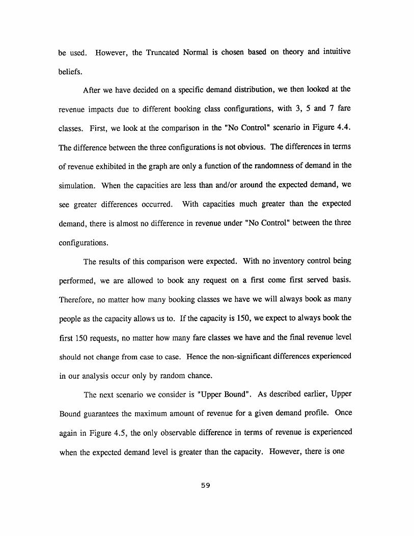
be used. However, the Truncated Normal is chosen based on theory and intuitive

beliefs.

After we have decided on a specific demand distribution, we then looked at the

revenue impacts due to different booking class configurations, with 3, 5 and 7 fare

classes. First, we look at the comparison in the "No Control" scenario in Figure 4.4.

The difference between the three configurations is not obvious. The differences in terms

of revenue exhibited in the graph are only a function of the randomness of demand in the

simulation. When the capacities are less than and/or around the expected demand, we

see greater differences occurred. With capacities much greater than the expected

demand, there is almost no difference in revenue under "No Control" between the three

configurations.

The results of this comparison were expected. With no inventory control being

performed, we are allowed to book any request on a first come first served basis.

Therefore, no matter how many booking classes we have we will always book as many

people as the capacity allows us to. If the capacity is 150, we expect to always book the

first 150 requests, no matter how many fare classes we have and the final revenue level

should not change from case to case. Hence the non-significant differences experienced

in our analysis occur only by random chance.

The next scenario we consider is "Upper Bound". As described earlier, Upper

Bound guarantees the maximum amount of revenue for a given demand profile. Once

again in Figure 4.5, the only observable difference in terms of revenue is experienced

when the expected demand level is greater than the capacity. However, there is one

Truncated Normal Distribution - No ControlComparing Number of Classes

150 170 190 210 230 250 270 290 310 330 350

Capacity

7 Classes 5 Classes M 3 Classes

Figure 4.4

60

Truncated Normal Distribution - Upper BoundComparing Number of Classes

45 I-

40 -

150 170 190 210 230 250 270 290 310 330 350

Capacity

7 Classes 5 Classes E 3 Classes

Figure 4.5

major observation that we can make here but not in the No Control case. The 5 and 7-

class configurations consistently exhibited (small) revenue advantages over the 3-class

configuration. This revenue advantage is at best around 3.18% better than the 3-class

configuration, and these advantages are mainly due to the following reasons. Since we

are booking the passengers with the highest yield (highest class) first, the more

segmentation we do, the better the overall revenue level, but this is only true when the

expected demand is greater than the capacity.

Once the capacity exceeds the expected demand, no matter how many different

booking classes we have, we will still allow the highest yield passengers book first up

to the capacity limit. Therefore, it will always be the same group of requests being

accepted when the capacity is greater than the expected demand. As we can see in

Figure 4.5, once the capacity exceeds the expected demand of 200, the advantage of

having more booking classes disappears and the total revenue values exhibits no statistical

differences. The minor differences shown in the graph are due solely to the randomly

generated demand and if the demands between different runs are the same or more

iterations are performed, these differences will be eliminated totally.

We have looked at the behavior of different number of inventory class

configurations under both the No Control and Upper Bound scenarios. What kind of

difference in terms of revenue can we expect in a seat inventory control environment?

Figure 4.6 shows the comparison of total revenues for the Expected Marginal Seat

Revenue model (EMSRb) over the three configurations. In this graph the distinction

between the three configurations is a little bit more precise, one can easily see the

Truncated Normal Distribution - EMSRbComparing Number of Classes

150 170 190 210 230 250 270 290 310 330 350

Capacity

7 Classes M 5 Classes M 3 Classes

Figure 4.6

63

40 "

revenue advantages of the 7-class over the 5-class and the 5-class over the 3-class

configuration. Although these revenue advantages are rather small, a point can still be

illustrated here. With inventory control, it is more obvious that the total revenue

increases as the number of classes increases. The reason for this to be true is very much

similar to the one given above for the Upper Bound scenario. When you are controlling

your seat inventory, one can be more selective in terms of which request to satisfy first

with a higher number of booking classes. Once again, this is only true when the capacity

is less than the expected demand. As soon as the capacity exceeds the demand, the same

group of requests will be satisfied no matter how many inventory control classes we use.

Table 4.11 illustrates the percentage difference between the 3 configurations under

the EMSRb seat inventory control scenario. The 7-class configuration is the clear

"winner" here, it shows up to 3.67% additional revenue over the 3-class configuration,

and up to 0.4% over the 5-class configuration at the lowest capacity, which translates

into a 133.33% demand factor. The 5-class configuration shows up to 3.29% higher

additional revenue over the 3-class case. As stated in the previous paragraph, these

additional revenues are only experienced when the expected demand is greater than the

aircraft capacity, when passenger requests are rejected. The 3.67% of additional revenue

for 7 classes compared to 3 classes represents an absolute difference of $1,634.46.

The next logical question one would ask is since all of these numbers look pretty

good, but do they have any statistical significance? Does the difference in revenue mean

anything, or it is just due to random occurrence? This question can be easily answered

by performing a simple statistical test. The test was done on the EMSRb scenario since

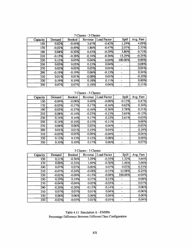
7 Classes - 3 Classes

Capacity Demand Booked Revenue Load Factor Spill Avg. Fare150 0.02% -0.44% 3.67% -0.42% 1.19% 4.09%170 -0.02% -0.49% 1.86% -0.47% 2.07% 2.33%190 0.04% -0.30% 0.43% -0.29% 3.80% 0.73%210 -0.15% -0.38% -0.74% -0.36% 15.29% -0.35%230 0.12% 0.05% 0.04% 0.04% 100.00% 0.00%250 0.05% 0.05% 0.12% 0.04% - 0.08%270 0.02% 0.02% 0.05% 0.01% - 0.04%290 -0.19% -0.19% 0.06% -0.13% - 0.24%310 0.01% 0.01% -0.08% 0.01% - -0.10%330 0.19% 0.19% 0.18% 0.11% - 0.00%350 0.07% 0.07% 0.18% 0.04% - 0.11%

7 Classes - 5 Classes

Capacity Demand Booked Revenue Load Factor Spill Avg. Fare150 -0.09% -0.08% 0.40% -0.08% -0.13% 0.47%170 -0.03% -0.17% 0.17% -0.16% 0.62% 0.34%190 -0.03% -0.37% -0.16% -0.36% 3.78% 0.21%210 -0.08% -0.14% -0.25% -0.13% 3.65% -0.12%230 0.14% 0.14% 0.17% 0.12% 2.61% 0.03%250 -0.14% -0.14% -0.15% -0.11% - 0.00%270 0.06% 0.06% 0.03% 0.04% - -0.03%290 0.01% 0.01% 0.19% 0.01% - 0.18%310 -0.05% -0.05% -0.09% -0.04% - -0.04%330 0.13% 0.13% 0.12% 0.08% - 0.00%350 0.10% 0.10% 0.179' 0.069' - 0.07%

5 Classes - 3 Classes

Capacity Demand Booked Revenue Load Factor Spill Avg. Fare150 0.11% -0.36% 3.29% -0.35%' 1.32% 3.64%170 0.00% -0.32% 1.69% -0.30% 1.46% 2.00%190 0.07% 0.07% 0.60% 0.07% 0.03% 0.53%210 -0.07% -0.24% -0.48% -0.23% 12.08% -0.24%230 -0.02% -0.09% -0.13% -0.08% 100.00% -0.04%250 0.19% 0.19% 0.27% 0.15% - 0.08%270 -0.04% -0.04% 0.02% -0.03% - 0.07%290 -0.20% -0.20% -0.13% -0.14% - 0.06%310 0.07% 0.07% 0.01% 0.04% - -0.06%330 0.06% 0.06% 0.06% 0.04% - 0.00%350 -0.03% -0.03% 0.01% -0.01% - 0.04%'

Table 4.11 Simulation A - EMSRb

Percentage Difference Between Different Class Configuration

it has the most interest to us with a inventory controlled environment. The test

performed is a simple t-test to see if the two revenue means are statistically different, and

the results confirm our discussion earlier. With the capacity level at 150 and 170, which

is less than the expected demand and a confidence level of 90%, the average revenues

are statistically different between the 7 and 3-class configurations and 5 and 3-class

configurations but not between 7 and 5-class. The differences have no statistical

significance once the capacity approaches the expected demand at capacity equal to 190

and beyond, and the results of the test agreed with Figure 4.6.

The revenue generated from different class configurations is now clear to us in

this simulation environment -- how about its impacts on some other measures such as

Load Factor and Yield? In terms of Load Factor, there are no obvious differences at all

in all of the inventory control methods between the number of booking classes. They all

follow a declining trend, as the capacity increases with the same expected demand, the

load factor decreases, which is rather obvious. Since our inventory control methods are

designed to maximize revenue rather than load factor, therefore, we should not expect

to see any difference in load factor within the same control method over different class

configurations.

Load Factors are the same for all different configurations within the same control

method, how about Yield? Since Yield is a direct derivative of Total Revenue and Load

Factor, and the load factors remain constant for different class configurations, we would

expect to see the same trends from the revenue discussion to emerge here.

We are using Average Fare instead of Yield in this analysis. Yield in the airline

industry is a function of Revenue, Passenger and Distance, but in our simulation we

assumed all passengers fly the same distance. Therefore, we can use Average Fare

rather than Yield here.

In the "No Control" case (Figure 4.7), just as in the revenue comparison, there

is no any significant difference between the number of class configurations. Based on

the first come first served rule, average fare will not be affected by class configuration

at all. The same arguments presented for the revenue discussion are still valid here.

When the classes are grouped together, a higher percentage of the total

reservations will be made in the bottom class with a lower revenue, therefore, the yield

(average fare) for the 3-class configuration is lower than the average fares for 5 and 7-

class. This can be observed rather easily from Figure 4.8. Due to the grouping

procedures and the relative fare structure between the 5 and 7-class configuration, no

obvious difference in terms of average fare is experienced. The findings in terms of

average fare section agree with the findings for total revenue. This is mainly due to no

difference in terms of load factors between the three different class configurations.

Last, we looked at the differences in average fare using the Expected Marginal

Seat Revenue (EMSRb) model for the three class configurations (Figure 4.9). As was

the case for the previous scenario, the same conclusions made with respect to total

revenue are still valid here. The average fare is highest with a 7-class configuration,

then the 5-class, and the lowest average fare was exhibited in the 3-class case. The 7-

class has a 0.47% advantage in terms of average fare over the 5-class and 4.09% above

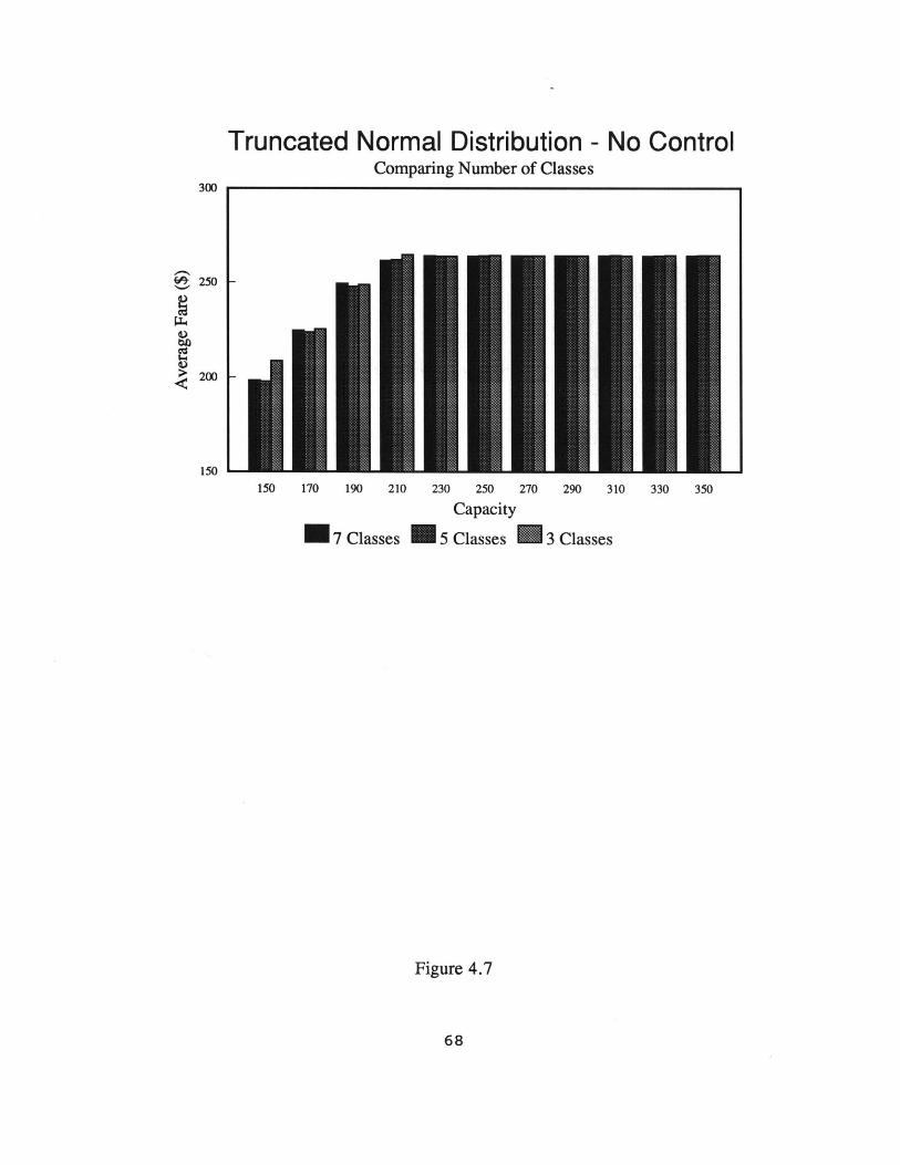
Truncated Normal Distribution - No ControlComparing Number of Classes

250 F

200 F

150 L-..150 170 190 210 230 250

Capacity270 290 310 330 350

7 Classes 5 Classes M 3 Classes

Figure 4.7

Truncated Normal Distribution - Upper BoundComparing Number of Classes

6 300

250

200

150 170 190 210 230 250 270

Capacity290 310 330 350

7 Classes 5 Classes M 3 Classes

Figure 4.8

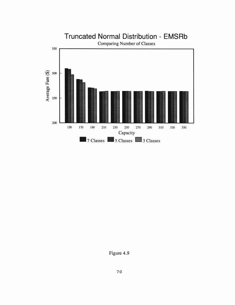
Truncated Normal Distribution - EMSRbComparing Number of Classes

150 170 190 210 230 250 270 290 310 330 350

Capacity

7 Classes 5 Classes 3 Classes

Figure 4.9

70

300

250

200

the 3-class configuration at capacity equal to 150 or demand factor equal to 133.33%.

In absolute terms, on average passengers in a 7-class booking system paid an additional

fare of over $12.00 per head than the average passenger from a 3-class system. This is

again significant to the airlines in terms of overall revenue. Once again, these

differences will only be experienced when the capacity is lower than the expected

demand. Once the demand is lower than the capacity these additional revenues will not

be realized by increasing the number of booking classes in the reservation system.

We have seen the differences between the number of class configurations in terms

of Revenue, Load Factor and Average Fare. But how much can a sophisticated 7-class

system buy us in terms of additional revenue over a 3-class system. This is rather

important to an airline who wishes to install a new revenue management system, since

it is better to do it right the first time than trying to change the existing system afterward

with regards to the number of classes.

One way to address this issue is to compare the revenue levels of an

inventory controlled environment (EMSRb) to the No Control scenario under a number

of different class configurations. Table 4.12 exhibits the percentage differences between

EMSRb and No Control under the three different class configurations. Just as the

previous discussions have shown, the differences between the 5 and 7-class configuration

are not very significant, but there is a 3% difference between the 3 and 7-class

configuration at low capacity when compared to the No Control scenario. Once again,

these revenue advantages appeared only when the expected demand is greater than the

capacity.

71

7 Classes

Capacity Demand Booked Revenue Load Factor Spill Avg. Fare150 -0.03% -4.31% 33.22% -4.13% 10.94% 35.98%170 -0.04% -3.84% 19.02% -3.70% 17.12% 22.01%190 0.05% -2.47% 5.77% -2.39% 28.13% 8.04%210 -0.08% -0.51% 0.14% -0.48% 29.00% 0.64%230 0.07% 0.05% 0.01% 0.05% 18.97% -0.04%250 -0.14% -0.14% -0.05% -0.11%/ - 0.09%270 0.12% 0.12% 0.10% 0.09% - -0.02%290 0.00% 0.00% 0.18% 0.00% - 0.18%310 0.02% 0.02% 0.02% 0.01% - 0.00%330 0.10% 0.10% 0.18% 0.06% - 0.08%350 0.03% 0.03% 0.08% 0.02% - 0.06%

5 Classes

Capacity Demand Booked Revenue Load Factor Spill Avg. Fare150 0.01% -4.22% 33.14% -4.05% 10.86% 35.85%170 0.11% -3.20% 19.56% -3.09% 15.16% 22.06%190 -0.10% -1.50% 7.07% -1.45% 16.11% 8.44%210 0.04% -0.44% 0.18% -0.41% 33.91% 0.62%230 -0.16% -0.23% -0.27% -0.20% 100.00% -0.04%250 0.07% 0.07% 0.13% 0.05% - 0.06%270 -0.07% -0.07% -0.04% -0.05% - 0.04%290 0.04% 0.04% 0.03% 0.03% - -0.01%310 0.01% 0.01% -0.03% 0.00% - -0.04%330 -0.19% -0.19% -0.18% -0.11% - 0.01%350 -0.059' -0.059' -0.149' -0.039' - -0.09%

3 Classes

Capacity Demand Booked Revenue Load Factor Spill Avg. Fare150 -0.05% 0.29% 30.02% 0.28% -0.92% 29.82%170 0.02% -3.31% 17.19% -3.20% 15.43% 19.84%190 -0.10% -1.96% 5.78% -1.90% 21.48% 7.59%210 0.05% 0.03% -0.10% 0.03% 1.96% -0.12%230 -0.09% -0.06% -0.05% -0.05% - 0.02%250 -0.07% -0.07% -0.13% -0.06% - -0.06%270 -0.06% -0.06% -0.12% -0.05% - -0.05%290 0.27% 0.27% 0.24% 0.19% - -0.03%310 0.00% 0.00% 0.06% 0.00% - 0.07%330 0.06% 0.06% 0.05% 0.03% - -0.01%350 -0.02% -0.029' -0.149' -0.01% - -0.12%

Table 4.12 Simulation A - EMSRb

Percentage Difference From "No Control" in Different Class Configuration

One of the main reasons for the minimum difference experienced between

different class configurations is probably due to the booking process used in this

simulation. With a single optimization and one period of demand booking, the benefits

of the higher number of classes and inventory control process might not be fully realized.

These benefits should be more obvious when we discuss the multiple period booking

process simulation in a later section.

One last thing we are going to look at before we leave the single optimization,

single period booking simulation is the impacts on revenue as a function of uncertainties.

We proposed a rather simple way to examine this point -- we simply modified the

standard deviations for each of the class demands in the input file by doubling and even

tripling the standard deviations and then performing the same simulations using these new

standard deviations and the sigma in the base case remains the root of the mean demand

during each demand period.

Since we have shown the 7-class configuration to give us the best revenue results,

only a 7-class case was studied in this context. The results of the simulation in terms of

percentage differences from No Control are presented in Table 4.13. As the uncertainty

increases the expected revenue decreases accordingly. The results are rather obvious,

since as the standard deviation increases, it is harder to "predict" and "protect" the

proper number of seats therefore, the revenue difference between inventory control and

No Control decreases.

In Simulation A, the Truncated Normal distribution was chosen based on its

ability to better generate expected demands. The selection was mainly based on intuition,

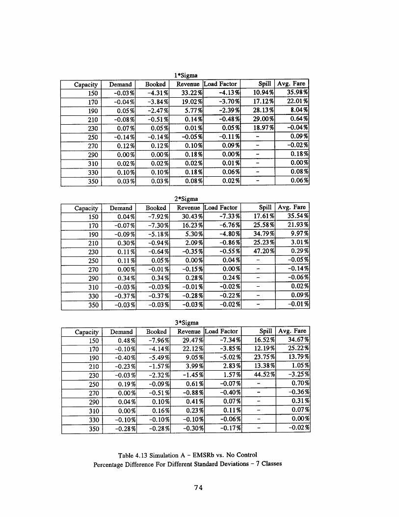
1*Sigma

Capacity Demand Booked Revenue Load Factor Spill Avg. Fare

150 -0.03% -4.31% 33.22% -4.13% 10.94% 35.98%

170 -0.04% -3.84% 19.02% -3.70% 17.12% 22.01%

190 0.05% -2.47% 5.77% -2.39% 28.13% 8.04%

210 -0.08% -0.51% 0.14% -0.48% 29.00% 0.64%

230 0.07% 0.05% 0.01% 0.05% 18.97% -0.04%

250 -0.14% -0.14% -0.05% -0.11% - 0.09%

270 0.12% 0.12% 0.10% 0.09% - -0.02%

290 0.00% 0.00% 0.18% 0.00% - 0.18%

310 0.02% 0.02% 0.02% 0.01% - 0.00%

330 0.10% 0.10% 0.18% 0.06% - 0.08%

350 0.03% 0.03% 0.08% 0.02% - 0.06%

2*Sigma

Capacity Demand Booked Revenue Load Factor Spill Avg. Fare

150 0.04% -7.92% 30.43% -7.33% 17.61% 35.54%

170 -0.07% -7.30% 16.23% -6.76% 25.58% 21.93%

190 -0.09% -5.18% 5.30% -4.80% 34.79% 9.97%

210 0.30% -0.94% 2.09% -0.86% 25.23% 3.01%

230 0.11% -0.64% -0.35% -0.55% 47.20% 0.29%

250 0.11% 0.05% 0.00% 0.04% - -0.05%

270 0.00% -0.01% -0.15% 0.00% - -0.14%

290 0.34% 0.34% 0.28% 0.24% - -0.06%

310 -0.03% -0.03% -0.01% -0.02% - 0.02%

330 -0.37% -0.37% -0.28% -0.22% - 0.09%

350 -0.03% -0.03% -0.03% -0.02% - -0.01%

3*Sigma

Capacity Demand Booked Revenue Load Factor Spill Avg. Fare

150 0.48% -7.96% 29.47% -7.34% 16.52% 34.67%

170 -0.10% -4.14% 22.12% -3.85% 12.19% 25.22%

190 -0.40% -5.49% 9.05% -5.02% 23.75% 13.79%

210 -0.23% -1.57% 3.99% 2.83% 13.38% 1.05%

230 -0.03% -2.32% -1.45% 1.57% 44.52% -3.25%

250 0.19% -0.09% 0.61% -0.07% - 0.70%

270 0.00% -0.51% -0.88% -0.40% - -0.36%

290 0.04% 0.10% 0.41% 0.07% - 0.31%

310 0.00% 0.16% 0.23% 0.11% - 0.07%

330 -0.10% -0.10% -0.10% -0.06% - 0.00%

350 -0.28% -0.28% -0.30% -0.17% - -0.02%

Table 4.13 Simulation A - EMSRb vs. No Control

Percentage Difference For Different Standard Deviations - 7 Classes

since the simulation results were inconclusive. We then used the Truncated Normal

distribution to perform the simulation and study the revenue impacts due to different fare

classes configurations. There is no significant revenue difference between different class

configurations under No Control and Upper Bound. However, with inventory control

(EMSRb) the higher the number of classes, the higher the total revenue although the

incremental differences diminish with more classes. We also compared the revenue

impacts of seat inventory control in a 3, 5 and 7-class configuration to No Control. The

additional revenue compared to No Control increases as the number of fare classes

increases. Last, we studied the issue of demand forecast uncertainty in our simulation.

As the standard deviation of the mean expected demand increases, the percentage revenue

increase from seat inventory control decreases.

4.2 Simulation B - Multiple Demand Periods, Single

Optimization

The first simulation we examined is a single demand, single optimization

simulation : Every class is booked as if all of the individual class demands arrive at one

instant. However, we know that this is not the case in the real world, where demands

come at different times in the booking process. Due to the restrictions applied to some

of the fare classes, the demands for different classes follow different arrival patterns.

The demand arrival pattern used in Simulation B and C is a close approximation of the

arrival pattern in the real world but is still aggregated into separate booking periods.

4.2.1 Description of Simulation B

The second simulation we used is a multiple period demand, single optimization

simulation. This simulation is done by using a simulation program written in the C

programming language, by the author as a tool for this study. The basic logic of this

simulation is similar to Simulation A, but the bookings procedures are slightly different.

In Simulation B, the expected demand arrives in the form of incremental demand.

As discussed previously in Chapter 3, these demands arrive by period for each booking

class. There are total of nine periods separated by revision points in our demand

scenario. The expected incremental demand along with the corresponding standard

deviation and average fare information for each booking class is contained in an input

file. This input file is used during the simulation process for calculating the fare class

booking limits at the beginning and to generate demands at each revision point.

Simulation B is a simplified version of the simulation used in the third analysis.

The details of the simulation will not be presented here. Only the major difference

between the two simulations will be discussed and the details of the complete simulation

are presented in Section 4.3. The major difference between Simulation B and Simulation

C is that in Simulation B, the seat inventory control process (setting booking limits) is

only executed once at the very beginning of the booking process. A set of booking limits

are calculated based on the total expected demand information, and as the incremental

demand comes in during subsequent periods, these limits are then simply reduced

according to the number of bookings accepted to date in each class. No recalculation of

booking limits is done in this simulation, hence, the actual booking information is not

used to feed a re-optimization of remaining capacity.

The decision rules used to determine if a generated demand should become an

actual booking remain unchanged from Simulation A. As a matter of fact, the same

booking decision rules are also used in the third and most sophisticated simulation.

4.2.2 Results of Simulation B

We to follow a similar structure for discussing the results from Simulation B as

for the first simulation. First, we examine the revenue difference between two assumed

demand distributions. Since we now have demand arriving in small intervals as

discussed earlier, it is more appropriate to assume that one of the distributions worth

testing is the Poisson distribution, and the second demand distribution remains the

Normal distribution. After we have selected one of the distributions as our standard

case, we will concentrate on the revenue differences between each of the three different

class configurations within each inventory control method.

We wish to establish which demand distribution pattern is more appropriate for

use in our multiple period demand case. Such a finding is important to us since we are

going to use this as the foundation for Simulation C to perform a more in-depth analysis

in terms of revenue differences between booking class configurations in a more realistic

airline reservation environment.

First, we look at the revenue differences between Poisson and Normal distribution

in the "Upper Bound" case. From Figure 4.10, we see the use of the Poisson

distribution in the simulation generates higher revenue estimates than the Normal

distribution. The revenue difference when capacity is less than mean total demand is not

as large as when the capacity is greater than the mean expected demand of 200. The

revenue difference starts at around 5 % with capacity equal to 150 and with capacity

greater than 190 the revenue differences are in the 10-11 % range.

Table 4.14 shows the differences in percentage terms between the Poisson and

Normal distribution assumptions. The Poisson distribution consistently generates 10%

higher demand when compared to the Normal distribution. Table 4.15 presents a

comparison between Normal and Poisson in absolute terms. The Normal distribution

consistently falls short of the target when trying to generate the predicted demand level.

With a target (expected total demand) of 200, the Normal distribution did not have an

average demand of over 183 under any capacity. This is due to the bias the Normal

distribution introduces when mean demands are relatively small, where negative demand

values are frequent occurrences. Based on this reason alone, we can reject the Normal

distribution over Poisson, but we will still look at the other scenarios -- No Control and

with inventory controls -- to strengthen our claim to choose Poisson over Normal in a

multiple demand simulation.

In Figure 4.11, we compare the revenue difference between the two demand

distribution assumptions under the No Control case. Just like the Upper Bound scenario,

the Poisson distribution exhibited a constant advantage over Normal but the differences

78

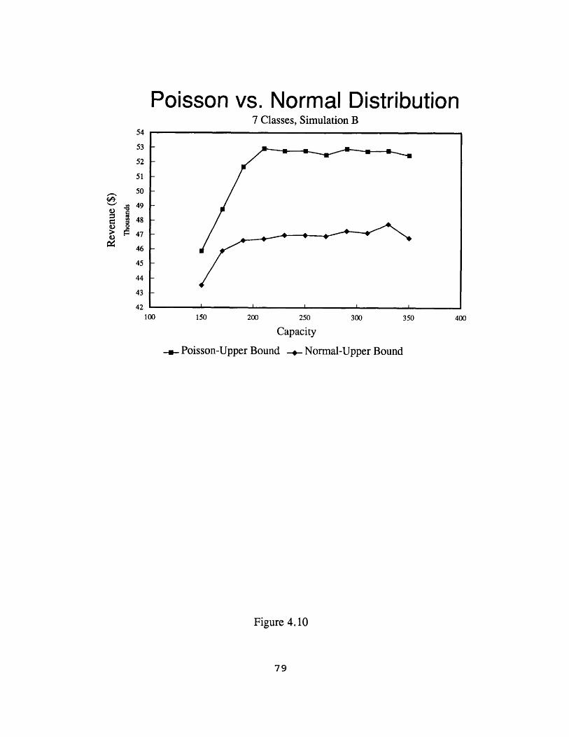
Poisson vs. Normal Distribution7 Classes, Simulation B

Capacity

-.- Poisson-Upper Bound -.- Normal-Upper Bound

Figure 4.10

79

/ .......,111 .....

Capacity Demand Booked Revenue Load Factor Spill Avg. Fare

150 9.39% 0.00% 5.13% 0.00% 36.77% 5.13%170 10.16% 1.36% 5.92% 1.36% 62.36% 4.66%190 11.94% 5.96% 9.82% 5.88% 85.70% 4.10%

210 11.17% 10.05% 11.72% 9.51% 100.00% 1.83%230 9.84% 9.84% 10.96% 8.51% - 1.21%

250 9.60% 9.60% 10.98% 7.59% - 1.48%

270 10.52% 10.52% 10.62% 7.76% - 0.13%

290 10.97% 10.97% 10.66% 7.59% - -0.38%

310 10.52% 10.52% 10.64% 6.75% - 0.24%

330 8.44% 8.44% 9.51% 5.10% - 1.19%

350 10.08% 10.08% 10.84% 5.74% - 0.91%

Table 4.14 Simulation B - Upper Bound, Poisson vs NormalPercentage Differences (P-N), 7 Classes

80

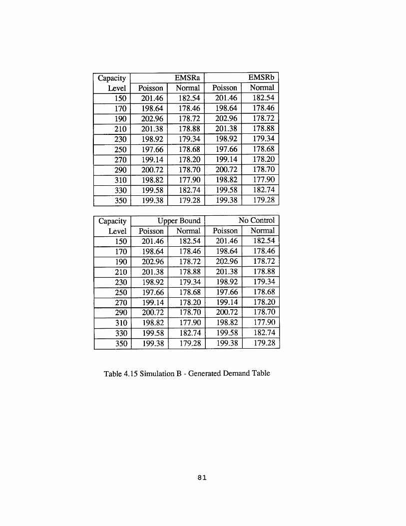
Capacity EMSRa EMSRbLevel Poisson Normal Poisson Normal

150 201.46 182.54 201.46 182.54170 198.64 178.46 198.64 178.46190 202.96 178.72 202.96 178.72210 201.38 178.88 201.38 178.88230 198.92 179.34 198.92 179.34250 197.66 178.68 197.66 178.68270 199.14 178.20 199.14 178.20290 200.72 178.70 200.72 178.70310 198.82 177.90 198.82 177.90330 199.58 182.74 199.58 182.74350 199.38 179.28 199.38 179.28

Capacity Upper Bound No ControlLevel Poisson Normal Poisson Normal

150 201.46 182.54 201.46 182.54170 198.64 178.46 198.64 178.46190 202.96 178.72 202.96 178.72210 201.38 178.88 201.38 178.88230 198.92 179.34 198.92 179.34250 197.66 178.68 197.66 178.68270 199.14 178.20 199.14 178.20290 200.72 178.70 200.72 178.70310 198.82 177.90 198.82 177.90330 199.58 182.74 199.58 182.74350 199.38 179.28 199.38 179.28

Table 4.15 Simulation B - Generated Demand Table

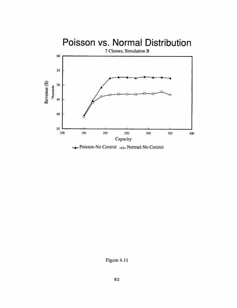
Poisson vs. Normal Distribution7 Classes, Simulation B

D 150 200 250 300 350 4

Capacity

-a- Poisson-No Control -.o- Normal-No Control

Figure 4.11

with capacity much lower than expected demand are very small (Table 4.15). This

minimum difference between the two distributions with low capacity levels is attributed

to the same reasons presented with the Upper Bound case. When the capacity is much

lower than the expected demand, the 10% negative difference in Normal tended to be

masked. This is especially true in No Control, due to the first come first served

philosophy. As long as the demand is greater than the capacity, the first group of

requests will be satisfied up to the capacity no matter what the final demand level is.

Once the capacity level is greater than the expected demand of 200, the revenue

difference started to increase and the percentage difference in terms of revenue is also

positively proportional to the difference in demands, as in Simulation A.

Figure 4.12 compares the case of EMSRb inventory control between Poisson and

Normal. Just as in Upper Bound and No control, the revenue advantage of Poisson over

Normal is obvious. Similar to the previous two scenarios, the "big" revenue advantage

was not fully realized until the capacity is greater than the expected demand, the reason

for this is the same as before, the under estimation of demand was masked by the fact

that the demand is so much greater than the capacity. Once the demand is close to or

less than the capacity, the 10% deficit in terms of generated demand by the Normal

distribution translated into 10% less revenue.

From the analysis of these three scenarios, it is rather easy for us to decide that

the Poisson distribution is definitely a better assumption in the simulation of multiple

demand arrivals, a conclusion that matches that introduced by Williamson1 for multiple

leg network simulation.

Poisson vs Normal Distribution7 Classes, Simulation B

150 200 250 300 350

Capacity

- Poisson-EMSRb -o- Normal-EMSRb

Figure 4.12

84

When we look at Figure 4.13-4.15, which compare the revenue differences

between the three different class configurations using the Poisson assumption, we see that

the results are not very conclusive. In the Upper Bound scenario, the 5 and 7-class

configurations have a slight advantage in terms of revenue over the 3-class configuration,

but in the case of No Control and EMSRb there are no statistically significant differences

at all. This is mainly due to the ineffectiveness of the static seat allocation methods to

capture the advantage of having more booking classes. Therefore, the significance of

having multiple booking classes in a multiple demand environment will be discussed in

the next section with the complete multiple optimization and multiple demand simulation.

The reason for selecting the Poisson distribution for multiple demand period

simulations is as follows. The Poisson distribution exhibits no bias in generating total

expected demand, given small mean demand values in each booking period. Due to the

properties of the Normal distribution, in each booking period with small mean demand

values the chance of generating negative demand is very high and it results in

consistently under estimating the total expected demand level. This bias would not be

obvious in Simulation A with only one booking period having mean expected demand of

200, but it becomes much more obvious once we introduce multiple period demand with

much smaller values in each booking period.

85

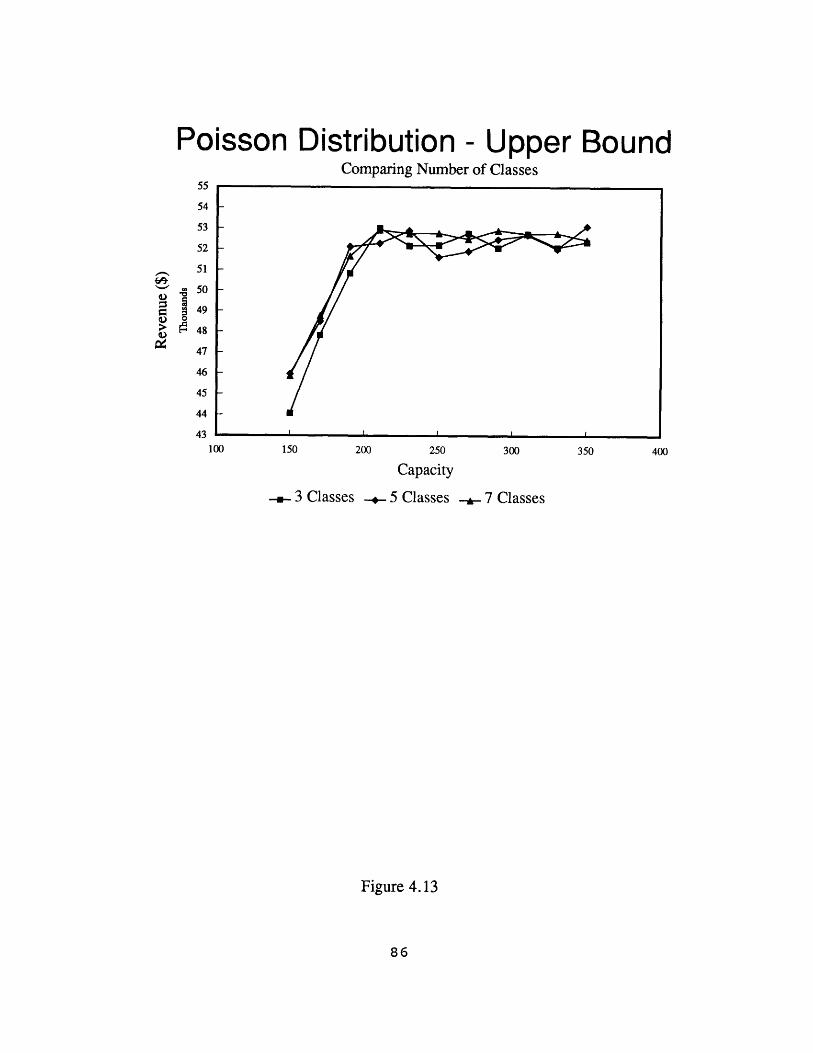
Poisson Distribution - Upper BoundComparing Number of Classes

150 200 250 300 350

Capacity

- 3 Classes . 5 Classes --. 7 Classes

Figure 4.13

86

Poisson Distribution - No ControlComparing Number of Classes

150 200 250 300 350

Capacity

-- 3 Classes - 5 Classes A 7 Classes

Figure 4.14

87

400

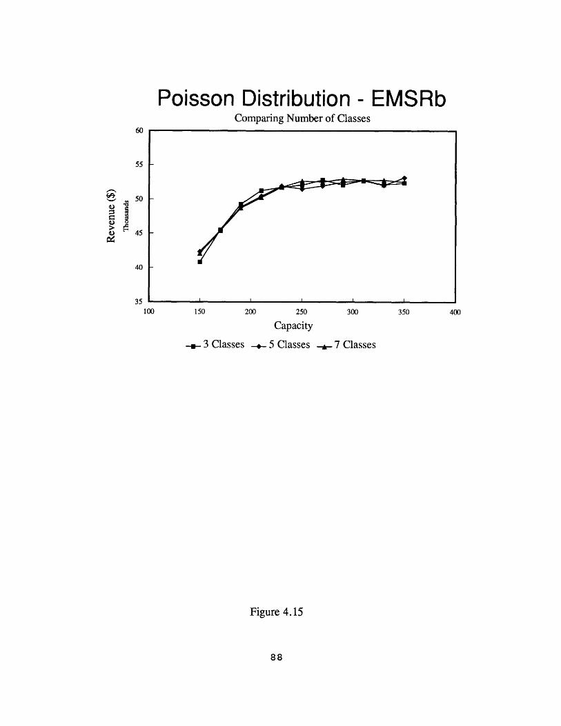
Poisson Distribution - EMSRbComparing Number of Classes

150 200 250 300 350 4

Capacity

-.-. 3 Classes -#- 5 Classes - 7 Classes

Figure 4.15

4.3 Simulation C - Multiple Demand Periods, Multiple

Optimization

The third and last simulation we examined is the most sophisticated one in this

study, as it simulates the booking process with multiple demand arrival periods and seat

allocation performed at each revision point between demand periods. Figure 4.16

presents the simulation in a pictorial manner.

4.3.1 Description of Simulation C

The simulation is a single leg-based simulation, meaning it is only concerned with

the booking process at a single leg level -- connection and through traffic are ignored.

By limiting the simulation to the single leg level the complexity of the analysis is reduced

drastically. In addition, an overwhelming majority of the airlines' reservation and seat

inventory control systems today are still in a single leg configuration.

In the simulation, the demands are generated randomly by a pseudo-random

number generator, based on the mean passenger demand in each fare class in each

period, which is assumed to follow a Poisson distribution. The booking process is

modeled to be a "Top-Down" booking procedure -- in contrast to the "Bottom-Up"

booking process used in Simulation A -- which means that in any given booking period,

the highest fare class is booked first. The simulation then books class number two and

No

or

Jppper LowerN

or

Figure 4.16

90

so on. The booking process for a particular demand period will end only if all of the

demands are satisfied and/or the capacity of the aircraft or booking limits has been

reached.

The simulation requires only one data input file as a data source. However, a

number of different variables are "hard coded" in the simulation and it is necessary to

change some of these variables to reflect the different situations being simulated. Such

variables are the number of fare classes, aircraft capacity and the number of revision

points

The demand and standard deviation for each fare class between each revision

point represents the expected incremental demand and standard deviation in that period

only -- it is neither total expected demand nor cumulative demand. The actual spacing

of these revision points was based on information obtained from an actual airline. Some

typical revision points are 3, 7, 14, 21, 35.. .etc. days prior to departure.

The main reason for having multiple revision points is explained by Belobaba2.

Using a number of revision points allows the airline to re-optimize booking limits given

information about actual bookings already accepted, thereby reducing the level of

uncertainty. Near optimal booking limits can be achieved with the EMSR methodology

by recalculating booking limits at each revision point. As the number of revision points

increases, the answer will approach the optimal solution.

There are basically two ways of generating sequences of random numbers for any

simulation. The first method is to simply "read" the random numbers from a list of such

numbers which has already been compiled by someone else. For example, a table with

one million random digits was published in 1955 by Rand Corporation3 . They can also

be obtained from mathematical tables, math textbooks, etc.

The second method (the one used in our simulation) is to have the computer itself

generate a sequence of random numbers. This is accomplished by having the computer

execute a short program every time a new random number is required. This computer

program essentially uses the last random number produced, say the (n-1)th in the

sequence, to produce the next random number, say the nth in the sequence. The

programming language used in this simulation is C and the specific method employed in

C is the Congruential Method. The congruential method uses the following expression

Xn = axn_1 + c (module m)

where X, and X. 1 are the nth and (n-1)th random numbers in the sequence, respectively,

and a, c and m are some suitably chosen positive integers with a < m and c < m. The

indication "module m" means that X, is the remainder of the division of the quantity aX..

1+c by the number m. In this case, a=1103515245, c=12345, and m=32767, a short

program returns a pseudo-random integer number which has a value between 0 to 32767.

We then divide each of the pseudo-random number by the largest possible random

number (32767) to achieve a sequence of pseudo-random numbers with values between

0 to 1. Since the passenger demand arrival pattern is assumed to have a Poisson

distribution in each booking period, the probability values for an event (a passenger's

request) happening in a given revision period are needed in order to calculate the total

demand in a given period. Hence, the use of pseudo-random numbers with values

between 0 and 1.

Consider the Poisson pmf P{N(T) =k}, which can be thought of as indicating the

probability of observing k events in a time interval T when inter-arrival times are

independent with a negative exponential distribution. To generate random observations

of N(T) for any given T, we follow the following procedure. We keep generating

exponentially distributed time intervals ti, ts2, t3 ... by using

-in (rn)

where rn is the random number generated earlier and lambda (X) is the mean historical

demand for a particular revision period.

This process continues until the total length of time represented by the sum of

these intervals exceeds T for the first time. That is, we find j such that

j j+1

i=1 i=1

then our sample observation of N(T) is given by k,=j (Figure 4.17).

Put into the context of our simulation, rn is the pseudo-random number generated

by the computer and then divided by 32767 to yield a number between 0 and 1, X is the

mean demand obtained from the input file for a particular booking period. By summing

up the events (passengers) arriving between t=0 and t=T, we can obtain the number of

passenger demands arrived in this period, which follows a Poisson process.

After demands have been generated in a demand period, the next logical step is

to book these demands against the booking limits calculated at the previous revision point

for each fare class. The booking limits are determined according to the methods

1st event

t T

-~ I

tsl - Ikffi,

ts2P-I -" ts3 I ts4

1i

ts5 I

T

Generation of random observations from Poisson distribution. In this figure, Ks = 4

Figure 4.17

tTOAOL AL4

I

3rd 4th 5th2nd

- I -

discussed in Chapter 3, and the booking process is then performed against these limits.

The booking processes programmed in the simulation follow a top-down approach, which

simply means that the highest fare class is booked first and then the second highest class

and so on within each individual booking period.

In order to translate demands to actual bookings, the following two conditions

must be satisfied,

SA1 = min(SA._1-BK_1, SA.)SAi Di

where SA; = Space Available for class i, except i =1;BKi = Bookings for Class i;

Di = Demands for Class i.

Space Available (SA) is essentially the booking limit in our booking process. At each

booking period, the randomly generated class demands become actual bookings based on

the space availability. SAs are re-calculated during each revision point, for the highest

booking class it is always equals to the remaining capacity of the aircraft at the revision

point, and for the rest of the fare classes it is based on the SA and nested protection level

of the immediately higher fare class.

The best way to understand the booking process is with a few examples. There

are two major cases, the first one occurs when the total demand for all classes during a

particular revision period is less than the remaining capacity of the aircraft. The other

situation arises when the opposite happens, i.e. when the total demand exceeds the

remaining capacity of the aircraft in a given revision period.

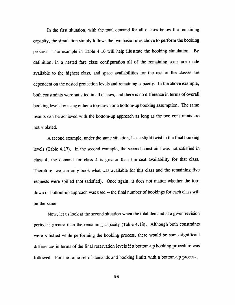
In the first situation, with the total demand for all classes below the remaining

capacity, the simulation simply follows the two basic rules above to perform the booking

process. The example in Table 4.16 will help illustrate the booking simulation. By

definition, in a nested fare class configuration all of the remaining seats are made

available to the highest class, and space availabilities for the rest of the classes are

dependent on the nested protection levels and remaining capacity. In the above example,

both constraints were satisfied in all classes, and there is no difference in terms of overall

booking levels by using either a top-down or a bottom-up booking assumption. The same

results can be achieved with the bottom-up approach as long as the two constraints are

not violated.

A second example, under the same situation, has a slight twist in the final booking

levels (Table 4.17). In the second example, the second constraint was not satisfied in

class 4, the demand for class 4 is greater than the seat availability for that class.

Therefore, we can only book what was available for this class and the remaining five

requests were spilled (not satisfied). Once again, it does not matter whether the top-

down or bottom-up approach was used -- the final number of bookings for each class will

be the same.

Now, let us look at the second situation when the total demand at a given revision

period is greater than the remaining capacity (Table 4.18). Although both constraints

were satisfied while performing the booking process, there would be some significant

differences in terms of the final reservation levels if a bottom-up booking procedure was

followed. For the same set of demands and booking limits with a bottom-up process,

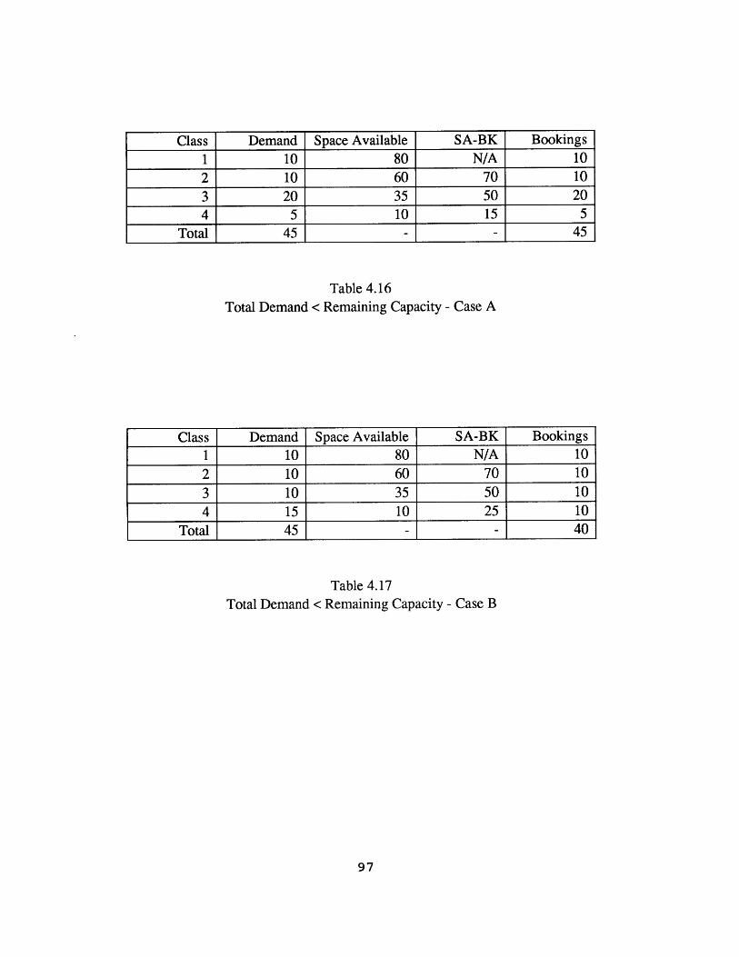
Class Demand Space Available SA-BK Bookings1 10 80 N/A 102 10 60 70 103 20 35 50 204 5 10 15 5

Total 45 - - 45

Table 4.16Total Demand < Remaining Capacity - Case A

Class Demand Space Available SA-BK Bookings1 10 80 N/A 102 10 60 70 103 10 35 50 10

4 15 10 25 10Total 45 - - 40

Table 4.17Total Demand < Remaining Capacity - Case B

Table 4.19 illustrates the differences in the final booking results.

The total number of reservations remains unchanged. However, there are ten

fewer bookings in class 2 and ten more bookings in class 4 as compared to the top-down

model. This discrepancy can arbitrarily make the total revenues consistently higher if

the top-down model is used, though on the other hand, the total revenue figure may be

too low if the bottom-up model is used. In real airline operations, the demand for

different classes does not arrive in any particular order within a single revision period,

therefore it is not entirely correct to assume either one of the two models.

This discrepancy can be resolved rather easily by using what is called the

"Proportional" booking method. Instead of booking demands from either top-down or

bottom-up, we will book only a certain percentage of the demand in each fare class when

total demand exceeds total space available, and this percentage is determined by dividing

remaining capacity by total demand

Booking Percentage = Remaining Capacity _ 80 - 0.80Total Demand 100

Table 4.20 exhibits the same example using the proportional booking method.

The proportional booking process can reduce the discrepancy incurred between

top-down and bottom-up booking processes, hence, it provides a more realistic revenue

estimate. The proportional booking method distributes the demands more realistically

over all classes, unlike the other two methods, which tend to concentrate the bookings

at either end of the fare class structure.

Class Demand Space Available SA-BK Bookings1 10 80 N/A 102 35 60 70 353 35 35 25 254 20 10 10 0

Total 100 - - 70

Table 4.18Total Demand > Remaining Capacity - "Top-Down"

Class Demand Space Available SA-BK Bookings1 10 80 N/A 102 35 60 N/A 25

3 35 35 N/A 254 20 10 N/A 10

Total 100 - - 70

Table 4.19Total Demand > Remaining Capacity - "Bottom-Up"

99

Class Demand Space Available Adjusted Demand SA-BK Bookings1 10 80 8 N/A 82 35 60 28 72 283 35 35 28 32 284 20 10 16 7 4

Total 1001 - 80 - 68

Booking Percentage = 0.80

Table 4.20Proportional Booking Example

100

In real life, the effects of inventory control adjustments on a particular flight can

be examined at most once. One of the many advantages of having a simulation is that

we can study the same flight over a number of artificial departures subjected to different

random demands, and due to the larger quantity and better quality of data available, any

trends, changes, and effects of the inventory control method can be examined

systematically.

Our simulation provides detailed outputs for further analysis; they are namely

demand, bookings and corresponding revenues at each departure for all departures at all

capacity scenarios. Based on these outputs, we can calculate two more important

parameters needed to study the revenue impacts of any inventory control process, Load

Factors and Yield.

Load Factors are calculated by dividing the number of bookings by the capacity.

It gives a sense of how full the aircraft was when it departed. Yield has always been

used when talking about airline performance, especially on Wall Street. In the airline

industry, yield is calculated by dividing total revenues by total passenger-miles : It is the

average revenue to the airline for carrying one passenger for one mile. In our simulated

environment, flight distances are irrelevant since they are assumed to be constant

throughout the study. Therefore, we simply divided revenues by the number of bookings

to arrive at an Average Fare. The next section will discuss the results from Simulation

C and examine the revenue impacts of revision.

101

4.3.2 Results of Simulation C

Based the second simulation, we have concluded that in a multiple period demand

process, it is more accurate to estimate the demand arrival pattern with a Poisson

distribution rather than using the Normal distribution assumption. We can examine just

one example in the multiple demand, multiple inventory control optimization case to

reinforce our conclusion from the previous simulation.

Since the inventory control scenario is the one we have the most interest in, we

consider only the EMSRb case. Figure 4.18 shows a comparison of revenues between

the Poisson and Normal distribution in a 7-class configuration with the inventory control

method being EMSRb. It is very obvious that once again the Poisson distribution

provides unbiased estimates of total demand in the case of multiple period demand with

small individual class means. Just like the previous simulation, the revenue difference

between the two distributions reaches its maximum once the capacity exceeds the

expected demand. The same reason given in the second simulation is still valid here,

when the capacity is less than the expected demand, the underestimate of the Normal

distribution was not fully realized due to the small capacity constraint. Once the capacity

exceeds the expected demand, the percentage difference in terms of revenue is in the

same magnitude of the percentage difference in generated demand. The Poisson

distribution is definitely more valid than the Normal distribution assumption based on the

negative bias towards small class mean demands exhibited by the Normal distribution.

The whole purpose of having both Simulation B and C is to examine the revenue

impacts of using multiple revision points in setting booking limits in a Dynamic situation

102

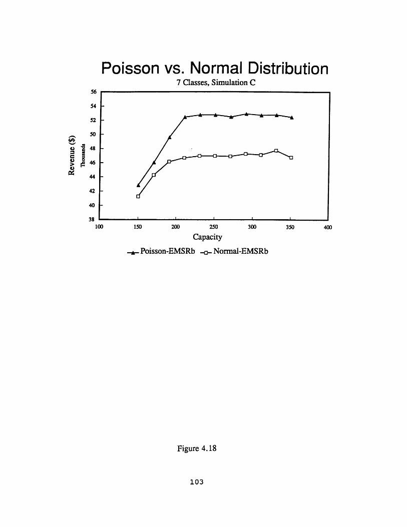
Poisson vs. Normal Distribution7 Classes, Simulation C

150 200 250 300 350

Capacity

.... Poisson-EMSRb -o- Normal-EMSRb

Figure 4.18

103

>

verse the Static case where the booking limits are set at the very beginning of the

booking process. We can consider the revenue impacts from the 3 different class

configurations.

Figure 4.19 compares the revenue differences between the static and dynamic seat

allocation methods in a 3-class configuration with the EMSRb seat inventory method.

The advantage of using the dynamic seat allocation method is not at all obvious in this

case. As a matter of fact, at capacities of 150 and 170, the revenue achieved using the

static seat inventory control method is marginally greater than the revenue resulted from

the dynamic seat allocation method. One reason for the revenue to be higher at the low

capacity level with static seat allocation is that when the capacity is low, the aircraft is

full before the expected "high" yield passenger arrives. With a 3-class configuration the

size of each class is bigger and the pool of remaining seats in the lowest class is also

bigger. Hence, the amount of time the lowest class is available for booking is longer

than the 5 or 7-class configuration, which may be why the dynamic case exhibited a

slightly lower revenue in the low capacity range. However, these differences are

statistically insignificant, in Table 4.21 the maximum revenue advantage occurred when

capacity is equal to 210 and as the capacity increases, the revenue starts to decrease.

This is true because, as the capacity increases, a higher portion of the demand will be

accommodated no matter which seat inventory control method is used, therefore, the

revenue difference diminished.

In the 5-class inventory structure, Figure 4.20, the dynamic seat allocation

exhibited better or same revenue results as the static case over all capacity levels. The

104

Static vs. Dynamic Seat Allocation3-Class Configuration, EMSRb

150 170 190 210 230 250 270 290 310 330 350

Capacity

-- Static -+- Dynamic

Figure 4.19

105

Capacity Demand Booked Revenue Load Factor Spill Avg. Fare150 0.00 0.00 -460.48 0.00% 0.00 -3.07170 0.00 0.00 -87.10 0.00% 0.00 -0.51190 0.00 2.76 455.59 1.00% -2.76 -1.68210 0.00 8.64 1426.20 4.00% -8.64 -4.69230 0.00 2.58 425.88 1.00% -2.58 -1.34250 0.00 0.80 132.06 0.00% -0.80 -0.38270 0.00 0.00 0.00 0.00% 0.00 0.00290 0.00 0.00 0.00 0.00% 0.00 0.00310 0.00 0.00 0.00 0.00% 0.00 0.00330 0.00 0.00 0.00 0.00% 0.00 0.00350 0.00 0.00 0.00 0.00% 0.00 0.00

Table 4.21 Simulation C - EMSRbStatic vs. Dynamic Seat Allocation

Absolute Differences (S-D)3 Classes

106

Static vs. Dynamic Seat Allocation5-Class Configuration, EMSRb

56

150 170 190 210 230 250 270 290 310 330 350

Capacity

-.- Static -.- Dynamic

Figure 4.20

107

-

revenue difference increases with the capacity until the capacity reaches the total mean

demand level. Once the capacity exceeds the total expected demand, the revenue

difference starts to decrease. When the capacity is much greater than the demand, the

revenue advantage of using dynamic seat allocation diminished. The maximum revenue

difference occurred at a capacity of 190 in this case, the dynamic seat allocation method

produces over $1300 in increased total revenue when compared to the Static case with

capacity equal to 190 or a demand factor of 105.26% (Table 4.22).

Figure 4.21 shows that in a 7-class structure the dynamic case again has a positive

revenue advantage over the static method for all capacity constraints. The same trend

that was exhibited in the 5-class situation is also observed here, with the absolute revenue

advantage increasing with the capacity until the capacity reaches the total expected

demand. Once the capacity exceeds the demand, the revenue difference decreases with

additional capacity until the revenue increase disappears. As before, once the capacity

is much larger than the demand, all of the demand will be satisfied no matter what kind

of inventory control method we are using.

In the 7-class configuration, the maximum positive revenue difference over the

Static case is in excess of $2200 when capacity is equal to 210 or a demand factor of

0.952 (Table 4.23) and this is the largest advantage we have experienced from the three

different class configurations. This difference in terms of revenue is wholly due to the

difference in booking class configurations, since all scenarios were subjected to the same

demand profile and identical random demand generation process. We now know that the

7-class configuration with the dynamic seat allocation method provides us with the "best"

108

Capacity Demand Booked Revenue Load Factor Spill Avg. Fare

150 0.00 1.98 912.67 1.00% -1.98 1.92170 0.00 8.90 795.71 5.00% -8.90 -11.60190 0.00 15.06 1366.23 8.00% -15.06 -16.59210 0.00 9.90 1291.51 5.00% -9.90 -7.49

230 0.00 7.18 970.55 3.00% -7.18 -4.91

250 0.00 1.12 152.46 0.00% -1.12 -0.71270 0.00 0.00 0.00 0.00% 0.00 0.00290 0.00 0.00 0.00 0.00% 0.00 0.00

310 0.00 0.00 0.00 0.00% 0.00 0.00330 0.00 0.00 0.00 0.00% 0.00 0.00350 0.00 0.00 0.00 0.00% 0.00 0.00

Table 4.22 Simulation C - EMSRb

Static vs. Dynamic Seat AllocationAbsolute Differences (S-D)

5 Classes

109

Static vs. Dynamic Seat Allocation7-Class Configuration, EMSRb

56

54

52

150 170 190 210 230 250

Capacity

-.- Static

270 290 310 330 350

-.#- Dynamic

Figure 4.21

110

I I I I | | I I I1|

|

Capacity Demand Booked Revenue Load Factor Spill Avg. Fare

150 0.00 4.42 782.24 3.00% -4.42 -4.65

170 0.00 11.18 678.16 7.00% -11.18 -16.72190 0.00 13.58 926.51 7.00% -13.58 -16.42

210 0.00 17.58 2238.57 8.00% -17.58 -14.29

230 0.00 7.72 1025.62 3.00% -7.72 -5.44

250 0.00 0.98 131.07 0.00% -0.98 -0.68270 0.00 0.00 0.00 0.00% 0.00 0.00290 0.00 0.00 0.00 0.00% 0.00 0.00310 0.00 0.00 0.00 0.00% 0.00 0.00330 0.00 0.00 0.00 0.00% 0.00 0.00350 0.00 0.00 0.00 0.00% 0.00 0.00

Table 4.23 Simulation C - EMSRb

Static vs. Dynamic Seat AllocationAbsolute Differences (S-D)

7 Classes

111

revenue advantage over the other two configurations using the same dynamic seat

allocation technique. However, we still have to look at the percentage difference from

the No Control case in all three class configurations before we can conclude which

configuration has the best overall revenue potential.

In Table 4.24, we can easily see that the number of classes definitely has an

impact in terms of revenue. The 7-class configuration has a maximum positive revenue

difference of 7.68% over No Control when subjected to the same demand, compared to

the 7.05% and 0.70% advantages the 5 and 3-class configurations have over No Control,

respectively. Since all of the cases are subject to the same demand, the differences are

real and solely attributable to having different numbers of booking classes. Once again,

as capacity increases the relative difference decreases. We accommodate most or all of

the requests for reservations, it does not matter what kind of seat inventory control

method is being used.

Based on the above analysis of Simulation C, we have once again confirmed the

selection of the Poisson distribution assumption over the Normal distribution in a multiple

period demand and multiple optimization simulation environment. When comparing

revenue impacts of different numbers of classes structure, 7-class configuration exhibits

higher revenue results over the 5 or 3-class configuration. Also, the impact of revisions

is a positive one in terms of total revenue. As we went from a Static seat allocation

process to the Dynamic seat allocation case, the total revenue increased. The revenue

differences between seat inventory control (EMSRb) and No Control also increases in

both absolute and percentage terms as the number of booking classes increases.

112

3 Classes

Capacity Demand Booked Revenue Load Factor Spill Avg. Fare150 0.00% 0.99% 0.70% 0.99% -3.05% -0.29%170 0.00% 0.81% 0.50% 0.81% -4.68% -0.31%190 0.00% 0.54% 0.34% 0.54% -7.86% -0.20%210 0.00% 0.07% 0.04% 0.07% -4.02% -0.03%230 0.00% 0.01% 0.01% 0.01% -6.67% 0.00%250 0.00% 0.00% 0.00% 0.00% - 0.00%270 0.00% 0.00% 0.00% 0.00% - 0.00%'290 0.00% 0.00% 0.00% 0.00% - 0.00%310 0.00% 0.00% 0.00% 0.00% - 0.00%330 0.00% 0.00% 0.00% 0.00% - 0.00%350 0.00% 0.00% 0.00% 0.00% - 0.00%

5 Classes

Capacity Demand Booked Revenue Load Factor Spill Avg. Fare150 0.00% 1.67% 7.05% 1.67% -5.02% 5.47%170 0.00% 1.07% 3.19% 1.07% -6.29% 2.20%190 0.00% 0.69% 0.85% 0.69% -8.03% 0.16%210 0.00% 0.09% 0.05% 0.09% -4.97% -0.04%230 0.00% 0.04% 0.02% 0.04% -36.36% -0.02%250 0.00% 0.00% 0.00% 0.00% - 0.00%270 0.00% 0.00% 0.00% 0.00% - 0.00%290 0.00% 0.00% 0.00% 0.00% - 0.00%310 0.00% 0.00% 0.00% 0.00% - 0.00%330 0.00% 0.00% 0.00% 0.00% - 0.00%350 0.00% 0.00% 0.00% 0.00' - 0.00%

7 Classes

Capacity Demand Booked Revenue Load Factor Spill Avg. Fare150 0.00% 2.48% 7.68% 2.48% -7.23% 5.34%j170 0.00% 1.99% 2.99% 1.99% -11.80% 1.02%190 0.00% 1.32% 0.77% 1.32% -16.02% -0.56%210 0.00% 0.08% 0.05% 0.08% -5.10% -0.02%230 0.00% 0.00% 0.00% 0.00% - 0.00%250 0.00% 0.00% 0.00% 0.00% - 0.00%270 0.00% 0.00% 0.00% 0.00% - 0.00%290 0.00% 0.00% 0.00% 0.00% - 0.00%310 0.00% 0.00% 0.00% 0.00% - 0.00%330 0.00% 0.00% 0.00% 0.00% - 0.00%350 0.00% 0.00% 0.00% 0.00% - 0.00%

Table 4.24 Simulation C - EMSRb

Percentage Differences From "No Control" in Different Class Configuration

113

1. Elizabeth Williamson, "Airline Network Seat Inventory Control: Methodologies and Revenue Impacts.", MIT Ph.D. Dissertation,forthcoming March 1992.

2. Peter P. Belobaba, "Air Travel Demand and Airline Seatinventory Management", M.I.T. Flight Transportation LaboratoryReport R87-7, 1987.

3. Richard C. Larson & Amedeo R. Odoni, "Urban OperationsResearch", Prentice Hall, Inc. 1981

114

Chapter 5

Revenue Opportunity Model and

Conclusions

5.1 Revenue Opportunity Model

In this section we apply the Revenue Opportunity Model introduced in Chapter

2. The analysis performed using this model is based on the simulation results obtained

from Simulation C -- multiple period demand, multiple optimization.

So far we have looked at the revenue impacts on airline yield management system

in the context of a number of different system configurations, such as Number-of-

Classes, Capacity Constraints, Static vs. Dynamic Seat Allocation. However, no detailed

comparison of the expected revenue impacts of inventory control methods was

performed. With the help of our simulation and the use of the Revenue Opportunity

Model developed by American Airlines Decision Technologies', we can study the

revenue impacts from different inventory control methods. With the combination of the

115

Revenue Opportunity model and the results from our simulation, it is much less sensitive

to external factors than other conventional methods used to measure revenue impacts such

as Yield and/or Load Factor, hence a true performance analysis between different control

methods can be studied.

The Revenue Opportunity Model measures the revenue performances of a

particular inventory control method as the percent of "Revenue Opportunity" achieved

by use of the inventory control method. Revenue performance is measured by using

"Upper Bound" to calculate the maximum possible revenue for the flight with perfect

information. This amount is the maximum revenue for the flight, next, we used the

results from the "No Control" analysis to calculate the revenue we would have earned

with no inventory controls. The revenue achieved from "No Control" is not the

minimum possible revenue without inventory controls, the reason being that we used a

"Top Down" approach within each booking period in our booking process in the

simulation as discussed previously. Since both EMSRa and EMSRb's booking processes

are performed by using the "Top-Down" approach, in order to keep a direct comparison

between all methods, the Top-Down approach was used through out our study. Based

on the Top-Down booking assumption, the revenue level of the "No Control" scenario

is slightly above the minimum if a Bottom-Up booking assumption was used, which

translated to a slightly more conservative performance advantage for the two inventory

control scenarios, namely EMSRa and EMSRb. However, since the booking process is

performed in small intervals, the impact of the "Top-Down" approach is not statistically

significant.

116

The difference between the minimum (No Control) and maximum (Upper Bound)

revenue is the total revenue opportunity that was available to us through the application

of inventory control. The amount of revenue opportunity achieved is determined by the

revenue earned from the EMSRa and EMSRb simulation results minus the minimum (No

Control) revenue. The performance of these inventory control methods is measured as

the percentage of revenue opportunity earned divided by the total revenue opportunity.

Figure 5.1 is a graphical representation of the Revenue Opportunity Model.

Table 5.1 exhibits the percentage of additional revenue opportunity achieved by

using EMSRa and EMSRb inventory control methods over no inventory control. The

highest amount of revenue opportunity was achieved with low capacity constraints. With

the aircraft capacity much lower than the expected demand of 200, EMSRa and EMSRB

achieved 53.32% and 52.13% of revenue opportunity respectively. As the capacity

increases, the revenue opportunity achieved decreases and once the capacity reached 230,

there are no more advantages in terms of additional revenue by using seat inventory

controls. With the capacity large enough to satisfy all requests, the advantages of using

inventory control diminished. In another words, the biggest revenue opportunity occurs

when the Demand Factor is much greater than unity. Demand factor is the ratio of

demand over capacity. When the demand factor is greater than one, spill may occur, and

when the demand factor is less than unity, a possible over capacity problem exists.

The revenue opportunities achieved by the two inventory control methods are very

similar, they both ranged at around 50% at capacity equal to 150 and reduced to the 5 %

level when the capacity reached 210. The reason for the different revenue opportunity

117

$ Revenue

&- Maximum Revenue

+ Actual Revenue

A Minimum Revenue

Revenue Opportunity Model

Figure 5.1

118

EMSRa EMSRb Upper Bound No ControlCapacity

150 53.32% 52.13% 100.00% 0.00%170 34.36% 33.78% 100.00% 0.00%190 17.31% 15.59% 100.00% 0.00%210 4.81% 5.89% 100.00% 0.00%230 N/A N/A N/A N/A250 N/A N/A N/A N/A270 N/A N/A N/A N/A290 N/A N/A N/A N/A310 N/A N/A N/A N/A330 N/A N/A N/A N/A350 N/A N/A N/A N/A

Table 5.1 Simulation CPercentage of Revenue Opportunity Achieved

119

achieved at different capacity levels is rather simple. At low capacity levels when the

expected total demand is much greater than the aircraft capacity, the advantage of

inventory control strategies to "choose and select" the right passenger mix is rather

important in terms of revenue opportunity. However, when the capacity is greater than

the expected demand, all of the randomly generated demand (requests) were satisfied,

both the needs and advantages of having a seat inventory control system became

unimportant.

5.2 Conclusions

The primary contribution of this research is the use of the single-leg based airline

booking simulation to study the revenue impacts of airline yield management system with

different constraints and configurations. The following findings are based on the results

of this research.

In a single demand period and single optimization booking simulation (Simulation

A), the preferred demand distribution is the Truncated Normal Distribution. The

selection process was not based solely on the results from our simulation, rather,

intuitively it also makes much more sense to use the Truncated Normal distribution in

order to avoid having negative demand values.

In terms of Revenue, there was not much difference in Simulation A between the

three different number of class configurations in both the No Control and Upper Bound

120

scenario. With inventory control - EMSRb, the 7 and 5-class configurations consistently

exhibited revenue advantages over the 3-class configuration.

In the inventory control case (EMSRb), the revenue increases as the number of

classes increases but this was only observed with relative small capacity levels and high

demand factors. Once the capacity had exceeded the expected demand total level, the

revenue difference between different configurations started to decrease. When the

capacity is much larger than the demand, the difference diminished. The last thing we

looked at in Simulation A is the effect of uncertainty in forecasting demand. The

expected revenue decreases as the magnitude of the standard deviation for the demand

increases in the EMSRb -- inventory control case with 7 booking classes.

The second simulation presented is a multiple demand period, single seat

allocation simulation (Simulation B). The prime purpose of this simulation is to select

a demand distribution for a multiple demand scenario. Since the demand arrives in small

intervals, the Normal or Truncated Normal distribution assumption became impractical

due to its bias in predicting small demand values. Based on the analysis of Simulation

B, we confirmed the Poisson distribution as the preferred demand distribution pattern for

a multiple demand arrival pattern.

Simulation C is the most sophisticated model of the three simulations used in this

research and is similar to a major U.S. carrier's reservation system. It is a single-leg,

multiple demand, multiple class, multiple seat allocation booking simulation. We

confirmed the selection of the Poisson distribution over Normal with a basic revenue

impact analysis based on the results from Simulation C.

121

The revenue advantage of having a multiple fare classes was also studied using

the results from this simulation. We have concluded that with the multiple demand,

multiple seat allocation simulation, the 7-class configuration outperformed the 3 and 5-

class configurations and similarly, the 5-class configuration has a better revenue

contribution than the 3-class case. With a higher number of fare classes, the ability of

segmenting potential passengers improved and hence better overall revenue results were

achieved.

Not only is the absolute revenue better with a higher number of fare/booking

classes, the incremental revenue achieved by using seat inventory control over the "No

Control" scenario also increases as the number of fare classes increase.

Finally, with a specified demand profile, the multiple demand, multiple seat

allocation simulation with a 7-class configuration outperformed any other cases in terms

of revenue impacts. Therefore, we conclude that based on the simulation results from

our research, the dynamic seat allocation with multiple revision points is better than the

static case since we can utilize the latest booking information after each revision period

in the multiple seat allocation case. EMSRb achieved up to 52.13% of the total revenue

opportunity when capacity is equal to 150 or a demand factor of 133.33% using the

results from Simulation C.

122

5.3 Future Research

For future research, one can combine the simulation program developed here with

the Revenue Opportunity model developed by AADT to study the revenue impacts from

using different inventory control methods. One possible idea is to study the revenue

difference between the two Expected Marginal Seat Revenue models (EMSRa and

EMSRb) mentioned above, and relative to Optimal Booking Limits (OBL). It is also

possible to study the revenue impacts incurred from actions taken by an inventory control

analyst. This can be achieved by simulating the analyst or using existing data of the

analyst from his/her daily operation.

With just the simulation program one can look beyond revenue -- the impacts of

Load Factor, Spill and Yield can also be studied. By improving the simulation, one can

also incorporate the use of different demand arrival patterns, overbooking factors, no-

show rates, cancellation rates along the booking process to study their respective impacts.

The possibility of future study with this simulation is great since the basic booking

process is replicated in a simulated environment.

1. Barry C. Smith, John F. Leimkuhler, Ross M. Darrow, "Yield Management At AmericanAirlines." American Airline Decision Technologies, 1989.

123