Revealing Urban Dynamics by Learning Online and Offline

30

Revealing Urban Dynamics by Learning Online and OfflineBehaviours Together

TONG XIA and YONG LI, Beijing National Research Center for Information Science and Technology,Department of Electrical Engineering, Tsinghua University, China

Urban problems and diseases accompanied by the pace of urbanization have drawn attention to the importance of understandingurban dynamics, while a deep and comprehensive understanding is challenging due to our diversified lifestyles in the moderncity. In this paper, we propose an urban dynamics modeling system to characterize the regularity of urban activity dynamicsas well as urban functions by learning residents’ online and offline behaviours together. Built on a state-sharing hiddenMarkov model, our system utilizes online activities of App usage and offline activities of mobility in different urban regionsand different time slots for learning. The learnt state sequence of each region reveals urban dynamics with the correspondingurban functions. We evaluate our system via a large-scale mobile network accessing dataset, which discovers ten hidden statescharacterizing different life modes and eight representative dynamic patterns corresponding to different urban functions.These discovered dynamic patterns and inferred functions are validated by social media check-ins and the land-use publishedby the government with 81% accuracy. Based on our model, we propose two applications, crowd flow prediction and popularApp prediction, which outperforms the state-of-the-art approaches by 36.1% and 15.7%, respectively. This study paves theway for extensive city-related applications including urban demand analysis, land-use planning, and activity prediction.

CCS Concepts: • Information systems → Spatial-temporal systems; Data mining; • Human-centered computing→ Empirical studies in ubiquitous and mobile computing; • Computing methodologies → Machine learning.

Additional Key Words and Phrases: urban dynamics modeling and revealing, online and offline behaviours, state-sharingHMM, mobile cellular network accessing dataset.

ACM Reference Format:Tong Xia and Yong Li. 2019. Revealing Urban Dynamics by Learning Online and Offline Behaviours Together. Proc. ACMInteract. Mob. Wearable Ubiquitous Technol. 3, 1, Article 30 (March 2019), 25 pages. https://doi.org/10.1145/3314417

1 INTRODUCTIONRevealing urban dynamics, i.e., how the types and intensity of human activities in the city change along withthe time, has always been a crucial social-economic task for both researchers and governments [2, 24]. Withthe ever-increasing urbanization process, human activities in the city are becoming increasingly dynamic andcomplex, making it more difficult to understand and model [16]. Moreover, nowadays human daily activitiesinclude not only the commuting between home and office, meeting friends, shopping, etc. in the physical space,but also the checking-in, liking the online friends, buying and selling goods, etc. in the cyberspace [7, 26],

This work was supported in part by the National Key Research and Development Program of China under grant 2017YFE0112300, the NationalNature Science Foundation of China under 61861136003, 61621091 and 61673237, Beijing National Research Center for Information Scienceand Technology under 20031887521, and research fund of Tsinghua University - Tencent Joint Laboratory for Internet Innovation Technology.Authors’ address: Tong Xia, [email protected]; Yong Li, [email protected], Beijing National Research Center forInformation Science and Technology, Department of Electrical Engineering, Tsinghua University, Beijing, China.

Permission to make digital or hard copies of all or part of this work for personal or classroom use is granted without fee provided thatcopies are not made or distributed for profit or commercial advantage and that copies bear this notice and the full citation on the first page.Copyrights for components of this work owned by others than the author(s) must be honored. Abstracting with credit is permitted. To copyotherwise, or republish, to post on servers or to redistribute to lists, requires prior specific permission and/or a fee. Request permissions [email protected].© 2019 Copyright held by the owner/author(s). Publication rights licensed to ACM.2474-9567/2019/3-ART30 $15.00https://doi.org/10.1145/3314417

Proc. ACM Interact. Mob. Wearable Ubiquitous Technol., Vol. 3, No. 1, Article 30. Publication date: March 2019.

https://doi.org/10.1145/3314417

https://doi.org/10.1145/3314417

30:2 • T. Xia and Y. Li

which are more high-dimensional and dynamic. Although uncovering the regularity of such daily activitiesis challenging, it is of great significance to tackle a series of urban problems, e.g., overcrowding, inadequateinfrastructure, traffic congestion, pollution, etc. [50]. What’s more, different kinds of dynamics are mainly causedby different land-use of the urban regions [45, 46], which indicates that revealing urban dynamics is directlyrelated with the inference of urban functions to facilitate better urban planning [31].Until now, most of our understanding about urban dynamics come from traditional surveys conducted by

human agents [25]. While this way of collecting data provides detailed information about urban behaviours, itremains hard to update and presents many weaknesses regarding generalization and geographical scope. Luckily,with the ubiquitous mobile devices, massive data recording various human activities is available to reveal urbandynamics. Recently, related works aim to uncover the temporal regularity of human activities, such as detectingthe patterns of mobility behaviours in the city via passive mobile positioning data [5], visualizing the level ofactivities at a given urban location across multiple temporal resolutions [2], etc. However, these existing studiesonly utilized offline behaviours for urban dynamics understanding by statistics and visualization methods, whichcannot realize specific and predictable human activity modeling.In this paper, our goal is to model urban dynamics with regard to human online and offline behaviours in

the city and further to infer urban functions. Despite its practical importance, using both online and offlineactivities is non-trivial due to three challenges: 1) Urban residents’ activities are dynamic and complex. Usingwhich kinds of online and offline features to characterize the activity type and intensity is the first challenge. 2)Underlying the various activities, there are several basic city states characterizing different life modes such asbusy working or peaceful sleeping, which compose urban dynamics. To model urban dynamics from the cityscale, similar activities, whether in the same or different regions, should be detected as the same state. However,on the other hand, though the states are the same, the dynamic patterns of different regions could be differentdue to their urban functions. Moreover, the data of each region would be limited to learn its own states anddynamics. Therefore, how to build one robust model to learn the difference as well as the similarity is the secondchallenge. 3) The relation between urban dynamics and urban functions is implicit, and the function of eachurban region could be single, compound, or even dynamic. How to infer it according to the learnt activity statesis the third challenge.To overcome these challenges, we propose an urban dynamics modeling system by leveraging the following

three key designs. First, we select human online activities of App usage and offline activities of mobility asfeatures. The intuitive motivations of utilizing these two features is that accessing to the Internet though Apps[1] and moving between different places [11] are the most important activities in the cyber and physical urbanspace, respectively. The App usage, i.e., how frequently the Apps are used, and the mobility, i.e., the volume ofcrowd flows, can reflect the type and the intensity of activities in a region. To extract these features, we utilizea mobile cellular network accessing dataset, which records when and where a user uses which Apps. Second,to model urban dynamics based on these features, we propose a state-sharing hidden Markov model (HMM).Regarding urban residents’ online and offline activities as time series, we aim to detect a common set of hiddenstates characterizing basic life modes in the city and to reveal urban dynamics by the transition among thesestates. Particularly, the state set is shared by all regions yet each region has its own state sequence. Throughthis strategy, similarity and difference among different regions are learnt at the same time, and the problem ofdata sparsity is also solved. Third, to infer and interpret the urban functions from the learnt state sequences, wedesign a clustering algorithm to divide these state sequences into several typical dynamic patterns, where eachpattern maps to a specific function. By combining the semantics of states in different time slots, the relationsbetween urban dynamics and functions are uncovered. To summarize, the contribution of our work is four-fold:


Revealing Urban Dynamics by Learning Online and Offline Behaviours Together • 30:3

(1) We investigate the problem of understanding urban dynamics using human activities in both physical andcyber space recorded by mobile cellular network accessing dataset. To the best of our knowledge, this isthe first study to utilize both online and offline behaviours to reveal urban dynamics.

(2) We propose a novel urban dynamics modeling system based on the state-sharing HMM, where the statescharacterized by the type and intensity of human activities are shared by all urban regions, but each regionhas its own state sequence. It achieves qualitative representations of urban dynamics as the transitionsbetween different states.

(3) We evaluate our method by a real-world large-scale dataset in Shanghai, China. We have learned tenhidden states and discovered eight typical dynamic patterns corresponding to different urban functions.These discovered dynamic patterns and inferred functions are validated by social media check-ins and theland-use published by the government with 81% accuracy.

(4) We design two applications based on our model, i.e., crowd flow prediction and popular App prediction.Extensive experiments demonstrate that our proposed state-sharing HMM outperforms the state-of-the-artapproaches by 36.1% and 15.7%.

2 RELATED WORKIn this section, we introduce the related from three perspectives: urban dynamics modeling, urban functionsinferring, and hidden Markov model with its application.Urban dynamics modeling. Urban dynamics, generally defined as how sociological indicators (e.g., the

population, the land use) change over time [9], can be divided into two aspects: long-term urbanization withsustained economic growth [22], and short-term anthropogenic changes and activity rhythms [2, 24, 48]. Wefocus on the latter one and our goal is reveal urban dynamics in terms of human activities with different typesand intensity. Relevant to our work, Zhang et al. [48] demonstrated that the activity volume of an area is notuniformly distributed across time, and different areas have different activity volume temporal distributions crossthe geo-tagged social data. Also using the geo-tagged data from Twitter, Sofiane et al. [2] built activity timeseries for different cities and found that close neighborhoods tend to share similar rhythms. Louail et al. [20]demonstrated that the city shape and hot-spots change with the course of the day. Fabio et al. [24] captured thespatio-temporal activity in a city across multiple temporal resolutions, and visualized different activity levels indifferent time slots. From the perspective of individuals, Clemente et al. [8] revealed different urban lifestyles viasequences of purchases and mobility behaviours by coupling credit card data with mobile phone data. In thiswork, we regard urban activities as time series and aim to reveal the daily regularity hidden in them. Differentfrom the existing works utilizing only offline activities, we model urban dynamics by learning online and offlineactivities together. Besides, different from the works based on statistical analysis [2] and data visualization [24],we propose a specific model, which achieves urban dynamics understanding and prediction at the same time.

Urban functions inferring. Traditional approaches to infer the actual land-use often rely on costly humansurveys, yet it is still coarse-grained and limited in geographical scope. Recently, with the availability of massivedata from different sources, efficient methods to infer urban functions have been proposed. Pijiaonowski et al.[28] utilized GIS data to model and predict the change of land-use in the city, while Lenormand et al. [15] applieda functional network approach to determine land use patterns from mobile phone records. Louail et al. [19]utilized origin-destination (OD) matrices to capture the structure of cities and showed that cities essentially differby their proportion of two types of flows: integrated (between residential and employment hotspots) and randomflows. Yuan et al. [43] compared urban function discovering results only based on static Points of Interest (POIs)data and based on both POIs and mobility pattern of taxicabs, which proved that mobility reflecting the commutehas a strong relationship with urban functions. Besides, Wang et al. [34] and Zhang et al. [45] showed that thetemporal traffic pattern and the activities recorded by check-ins also can be utilized to infer urban functions. Our



work aims to infer the functions by the discovered dynamic patterns via a large-scale mobile cellular networkaccessing dataset. Moreover, unlike previous works to identify fine-grained yet static urban functions, we paymore attention to the composition of a region’s functions with its dynamic changes.Hidden Markov model and its application. Hidden Markov Model (HMM) is a statistical model in which

the time series being modeled is assumed to be a Markov process with unobserved (i.e., hidden) states[29].In order to improve the performance of HMM, parameter sharing are very helpful to deal with increasinglycomplex tasks [12]. One well-known example is shared-distribution HMM , where clustering is carried out atthe distribution level and output distributions are shared with each other if they exhibit acoustic similarity [14].Another example is tied-mixture HMM, which is a kind of semi-continuous HMM [3, 13, 17]. It assumes that eachoutput is generated by large amount of continuous probability density functions (PDFs), while the weight of thePDFs are discrete. By enforcing PDF sharing, it is able to improve the modeling accuracy as its fully using of data.Our proposed state-sharing HMM is also a kind of parameters sharing HMM. Unlike shared-distribution HMM, ourmodel can be learned end-to-end, which means no following clustering is need to force the parameters shared.Also unlike tied-mixture HMM, our model is designed to share a set of states which generates the continuousobservations directly instead of only sharing underlying PDFs.

HMM and its variants are also widely used in human activity modeling. One important application is individualmobility prediction [23, 47, 52]. These works assumes that a user’s movement is actual the successive transitionon several hidden states. These states are the key places he visits frequently (e.g, his home, his office, etc.). Theobserved spatial points are distributed around the key locations. Therefore, HMM is suitable to first determine thekey states under the trajectory, and than predict the next location the user would visit based on the state transitionprobability. Compared with the existing works, the novelty of our study lies applying HMM in urban dynamicsrevealing problem. We regard urban dynamics as the transition between hidden states which characterize humanactivities with different types and intensity, and we also achieve urban dynamics prediction.

3 PRELIMINARIES

3.1 MotivationsIn order to reveal urban dynamics in terms of daily activity rhythms, we investigate the variations of theaggregated online and offline activities along with time. In this section, we discuss the motivations to selectmobility as offline activity feature and App usage as online activity feature.Human mobility, reflecting daily life pattern by its distinct modes, is the most important social-economic

activity in the physical space [38]. Consequently, the aggregated mobility behaviour, i.e., how many people leavefrom, arrive at and stay in each urban region and time slot, reflects urban commuting patterns, indicating that itshould be used as offline feature for urban dynamics modeling [42].

While in terms of online activities, it is recently reported that more than 80% of the mobile phone using time inall markets are spent in Apps [1], which demonstrates the purpose of accessing the Internet could be reflected bythe App usage. Moreover, the App usage varies significantly with the regions of different land-use, which indicatesit has a strong correlation with urban functions [41]. Utilizing the mobile cellular network accessing dataset,we also explore the correlation between App usage and land-use explicitly. As Figure 1(a) shows, App usage inthe regions with different land-use are obviously different, which reflects people’s different App preferences indifferent places. We also show the cumulative distribution function of the statistical correlation between land-usecomponents and App usage in Figure 1(b). The results show that for more than 80% of the regions, they arestrongly correlated (above 0.76). Therefore, we utilize App usage as online bebaviour representation to modelurban dynamics and infer urban functions.



(a) For different types of regions (i.e. regions with relatively higherfrequency of certain types of land-use), we calculate the percentageof different App categories used.

(b) Cumulative distribution function of the statistical corre-lation between App usage and the the land-use.

Fig. 1. Intuitive and statistic correlation between App usage and land-use.

3.2 State-sharing HMMRegarding the App usage and mobility features in different time slots as time series, we are able to apply HMMto reveal urban dynamics. To deal with the problem of data sparsity and to detect similar as well as differentdynamics of urban regions, we propose a state-sharing HMM. Before formally defining the model, we give anexampled illustration in Figure 2.

(a) States and transition probabilities (b) State sequences of two different regions

Fig. 2. An exampled illustration of the state-sharing HMM, where five states with different semantics are shown in fivecircles of different colors, and their transition probabilities are represented by the colorful arrows. As shown in (a), the thickerthe line is, the greater the probability is. Two state sequences of different regions in a working day are shown in (b), where Ais a residence region and B is an office region.

In this example, S0, S1, S2, S3 and S4 are five hidden states characterizing human online and offline activitieswith different types and intensity. S0 denotes the state with low activity intensity both in App usage and mobility.S2 denotes the state that few people are moving and relaxing Apps are used most frequently, while S3 denotesthe state that few people are moving and official Apps are used most frequently. Both with few Apps used, S1denotes a sudden moving-out crowd flow yet S4 denotes a sudden moving-in crowd flow. Besides, S0, S2 and S3



Fig. 3. Framework of the proposed system for urban dynamics modeling.

have larger probability of turning to themselves, Thus, they could continue to appear in a long period beforejumping to another state. Compared with S2 and S3, S1 and S4 have smaller probability of turning to themselves.Thus, they are more likely to appear in a rather short period. For each each urban region, these states appearin turn, which compose its state sequence. There are two different state sequences based on the common setof states and the same transition probabilities as shown in Figure 2(b). The sequence of region A, a residentialregion, shows the dynamics that few people are active at night, many people leave in the morning, shoppingApps are used most frequently during the day, and many people go back in the afternoon. On the contrary, thesequence of region B, which is an official region, shows the dynamics that many people arrive in the morning andleave in the afternoon, and use stock Apps instead of relaxing ones frequently during the day. To summary, statesare shared but state sequence is unique for each region, which represents the different urban dynamics. The goalof this paper is to discover the shared state set for the city, and own states state sequence for each region.

3.3 Problem Statement and Solution OverviewBased on the ideas discussed above, we formally define the urban dynamics modeling problem. Given the onlineand offline activity observations of different regions in the city, we aim to address the following three aspectsregarding urban dynamics: First is to discover the hidden states in the city, which characterizes human activitieswith different types and intensity. Second is to detect urban dynamic patterns, which is revealed by the hiddenstate sequence and could be mapped to urban functions. Third is to predict urban dynamics. Specifically, it is topredict the crowd flows and the popular Apps for each region in the next time slot.

We show the framework of our proposed system in Figure 3, which includes four modules named Preprocessing,Modeling, Annotation and Application. Specifically, we first extract App usage and mobility as the input featuresfor each region in different time slots from the mobile network accessing records. Then, we fed them into thestate-sharing HMM to discover the city states. Based on the HMM, we learn the state sequence of each region,which reveals the urban dynamics and functions. Besides, applications of predicting the crowd flows and popularApps can be achieved based on the model.

4 METHOD

4.1 PreprocessingMobile cellular network accessing data records when and under which base station a user is using which Apps.To detect the dynamics of urban regions, which are segmented by the major road networks, the first step is to



extract aggregated App usage and mobility features from individual records. For convenience, we discretize oneday into several time slots. To distinguish them in the working and non-working day, we use index [1,n] for theformer and [n + 1, 2n] for the latter. After mapping the base station to the region and change the timestamp tothe time slot, the i-th record is denoted by < ui ,τi ,дi ,ai >, where ui is the user ID, τi is the time slot and дi is theregion ID. In the following parts, we denote the set of users asU = {u1,u2, ...,uM }(1 ≤ m ≤ M), the set of regionsas G = {д1,д2, ...,дR }(1 ≤ r ≤ R), and the set of time slots as T = {τ1,τ2, ...,τN }(1 ≤ n ≤ N ), respectively.

4.1.1 Preprocessing for App Usage. Given a urban region, we define the App usage as how many people areusing a certain kind of Apps during one time slot. For the whole city, it is denoted as a 3-dimensional tensorX ∈ RR×N×La , where R is the number of regions, La is number of App categories, and N is the number of timeslots. Since different Apps in the same category play similar roles in reflecting human activities, we only use theApp category to characterize the type of human online activities. To share the states in the city, we normalize theApp usage to eliminate the influence of the population in different regions. We first compute the TF-IDF weightsfor the usage in each time slot. TF-IDF [27], short for term frequency-inverse document frequency, is a numericalstatistic that is intended to reflect how important a word is to a document in a collection or corpus. Here, we usethe TF-IDF weight to indicate how popular an App category is in the given time slot. The TF-IDF weight for then-th time slot denoted by Xn can be calculated as follows,

Xn(r , l) =X (r ,n, l)∑X (r ,n, :)

× log∑X (:,n, :)∑X (:,n, l)

. (1)

Then, for each region we conduct the max normalization on the weights over different time slots as follows,

X (r ,n, l) = Xn(r , l)/ max1≤n≤N ,l ≤l ≤L

(Xn(r , l)), (2)

where X denotes the normalized App usage tensor.

4.1.2 Preprocessing for Mobility. A user’s trajectory is defined as the base station sequence he has visited in timeorder. By traversing the trajectories of all users, we can obtain the mobility features that how many people leavefrom, arrive at and stay in each region in different time slots [49]. We denote the mobility features as Lr , Ar andSr , where Lr = (Lr,1,Lr,2, ...,Lr,N ), Ar = (Ar,1,Ar,2, ...,Ar,N ) and Sr = (Sr,1, Sr,2, ..., Sr,N )(1 ≤ n ≤ N ) with Lr,n ,Ar,n and Sr,n denoting the number of people who leave from, arrive at and stay in the r -th region in n-th timeslot, respectively. Similar with App usage, considering the difference for land area and population, we normalizedthese three vectors by their maximum value. The normalized mobility features denoted by Lr , Ar and Sr can beobtained as follows:

Lr,n = Lr,n/ max1<n<N

(Lr,n),∀n = 1, 2, ...,N ,∀r = 1, 2, ...,R, (3)

Ar,n = Ar,n/ max1<n<N

(Ar,n),∀n = 1, 2, ...,N ,∀r = 1, 2, ...,R, (4)

Sr,n = Sr,n/ max1<n<N

(Sr,n),∀n = 1, 2, ...,N ,∀r = 1, 2, ...,R. (5)

4.2 Modeling4.2.1 State-sharing Hidden Markov Model. For r -th region, we define the observation sequence from the onlineand offline activities as Or = Or,1Or,2...Or,n ...Or,N , where Or,n denotes the observation in n-th time slot. It isa multi-dimensional feature vector denoted by Or,n = ⟨or,n,1,or,n,2, , ...or,n,l ...or,n,L ⟩(L = La + 3) with or,n,l



presenting observation for App usage from X as (1)-(2) and mobility as (3)-(5) as follows:

or,n,l =

X (r ,n, l), 1 ≤ l ≤ La ,

Ar,n , l = L − 2,Lr,n , l = L − 1,Sr,n , l = L.

(6)

Observation sequence set of the city denoted by O = {O1,O2, ...,OR } is the input of our model, and our goalis to learn the corresponding hidden state sequence under them. We define the common state set including Khidden sates as S = [s1, s2, ..., sK ]. We assume that all the input observationsO are generated by these states. As ageneral practice for HMM, the observation variables on,l , (l = 1, 2, ...,L) are independent and on,l is generatedfrom Gaussian, i.e., p(on,l |sn = k) = N (µk,l ,σk,l ), where µk,l and σk,l are the mean and variance for hidden statek . Therefore, we build the state-sharing HMM parameterized by θ = {π ,A, µ,σ }, where:

(1) π ∈ RK×1 denotes the initial distribution over K hidden states, i.e., πk = p(s1 = k)(1 ≤ k ≤ K);(2) A ∈ RK×K denotes the transition probabilities among the K hidden states. If (n − 1)-th state is sn−1 = j,

then the probability for n-th state sn to be k is given by Aj,k , i.e., p(sn = k |sn−1 = j) = Aj,k ;(3) µ,σ ∈ RK×L denotes themean and variance of observation probability, i.e.,p(or,n,l |sn = k) = 1√

2πσk,lexp (− (or ,n,l−µk,l )2

2σk,l ).

4.2.2 Model Training. The model parameters θ = {π ,A, µ,σ } can be learned by maximizing the likehoodfunction, i.e., the probability of the observations represented by human activities for all regions under differenthidden states. According to Baum-Welch algorithm [29], the likehood function can be maximized by optimize theQ-function step by step. Therefore, the key of the parameter inference is to identify the Q-function denoted by:

Q(θ ,θ t ) =∑S

p(S |O ;θ t ) lnp(O, S |θ ), (7)

which is different from a general HMM. In our model, we need to maximize the likehood function of all regionsat the same time. Thus, Q function can be defined as follows,

Q(θ ,θ t ) =R∑r=1

∑S

p(S |Or ;θ t ) lnp(Or , S |θ ). (8)

We train the model using Expectation-Maximization (EM) algorithm [4], which is described in detail inAppendix I. Starting with random initialized parameters, EM algorithm alternates between E-step and M-stepround by round until the stop condition is satisfied. In the (t + 1)-th round E-step, it computes Q(θ ,θ t ) =R∑r=1

∑Sp(S |Or ;θ t ) lnp(Or , S |θ ). In M-step, it finds a new estimation θ (t+1) to maximizes Q-function. After several

rounds of iteration, the model tends to converge with the output of parameters θ = {π ,A, µ,σ }.

4.2.3 State Sequence Learning and Clustering. After model training, we obtain K hidden states parameterizedby {µ,σ } and the transition probability parameterized by θ = {π ,A}. Therefore, we can learn the hidden statesequence under each observation sequence Or by Viterbi algorithm [33]. As discussed before, the common statesset characterizes the fundamental life modes in the city, which reveals the similarity among different regions,while the hidden state sequence of each region indicates the uniqueness of its own dynamics.

In order to detect typical dynamic patterns, we further cluster urban regions according to their state sequences.To divide the regions with similar dynamics into the same cluster, we measure their distance by Hammingdistance of their state sequences [10]. Specifically, we define the distance of each two state sequences as thenumber of different states they have in the corresponding time slots. For example, as shown in Figure 2, states ofthese two region in 2-th, 3-th and 4-th time slot are different, thus the distance is 3. Because states are discrete



(a) Cumulative distribution of the number ofrecords for each user

(b) Usage for each App category (c) Spatial distribution for differentregions

Fig. 4. Data overview.

and cannot be averaged, we apply K-mediods algorithm for clustering [38]. K-mediods defines the intra-clusterdistance as the average of other regions to the center. Unlike K-means, it selects one region from all with theminimized intra-cluster distance as the cluster center in each round. To determine how many patterns are suitable,we adopt Davies-Bouldin index (DBI) [6] to determine the number of clusters, which reflects the ratio betweeninter-cluster distance and intra-cluster distance. A smaller DBI usually indicates a more effective clustering. Sincepeople attend different activities in the places with specific urban functions, the discovered states and dynamicpatterns are closely related to urban functions. Therefore, we can map dynamic patterns into urban functions.

5 EXPERIMENTSIn this section, we set up a series of experiments to evaluate our proposed model. We first introduce the useddatasets and the parameters. Then we discuss the learned dynamics and inferred functions in details. After that,we evaluate the the performance of our proposed application.

5.1 Datasets1) Mobile cellular network accessing data.We use this dataset to extract human online and offline activityfeatures. This dataset containing mobile users’ accessing logs to the cellular network is collected by collaboratingwith a major mobile network operator in Shanghai, China from April 20th to 26th, 2016. Through deep packetinspection, each access record is characterized by an anonymized user ID, timestamp, cellular base station withGPS location and the metadata of the networking communication. With the geographical information of cellularbase stations, we can recover users’ trajectories and further to extract offline mobility features. Beside, we canalso identify Apps from the networking metadata by adopting SAMPLES [40] to extract online App usage.Overall, the dataset contains over 1,700,000 unique devices, 2000 unique Apps, and 9800 base stations in

Shanghai. We divide these Apps into 9 categories by referring to the App Store (iOS Apps) and Google Play(Android Apps), which includes social, music, reading, game, shopping, restaurant, navigation, office, and stock.The cumulative distribution of the number of records for each user is shown in Figure 4(a). It shows that morethan 40% of the users are highly active with than more 200 records. The frequency of mobile users accessingdifferent App categories is shown in Figure 4(b), where App category is arranged in descending order of usingfrequency. This figure indicates that all kinds of App are used for more than 10 million times in one week and themost popular category is social. This large-scale and fine-grained dataset enables the representative of our study.

2) Road network. The road network data is used to obtain the boundaries of urban regions. Urban regionssegmented by roads are the basic geographic units of residents’ daily life and we use them to reveal urban



dynamics. We crawled the road network from the online map service. Using the major roads of high way andring roads, Shanghai is divided into 1595 non-overlapping regions spontaneously. Their distribution is shown inFigure 4(c). From this figure we can observe that the regions in downtown are fine-grained and those aroundsuburb are coarse-grained.3) Check-in dataset.We utilize social-media check-ins in different time slots to validate the uncovered urban

dynamics. Check-in refers that a user records his activity with the location information using smartphones [51].We collected this dataset from one of the most popular location-based sevice provider in China. Each check-inrecord consists of anonymized user ID, check-in time, check-in location and point of interest (POI). Totally, itcontains over 130,000 records appearing in Shanghai and covers the POI categories including entertainment, hotel,shopping, leisure, fitness, school, tourism, transportation, finance, company, business, factory, industry, technologypark, economic development zone, high-tech development zone, residence, life service, township and village.

4) Land-use map. We use this dataset to validate the inferred urban functions. We collected the latest urbanland-use planning map from the government, which contains six land-use types including residence, business,industry, public infrastructure, framing and forestry, and ecological restoration.Ethics. We have carefully considered the ethical issues of the data and taken effective measures to protect

users’ privacy by referring to previous related works which also utilized massive individual data [32, 41]. First,when the users use the network service provided by the cellular network operator or social-media platform,they have authorized that their data can be collected and analyzed by the provider. Moreover, all the personalidentification information have been stripped (or replaced by a random string) by the provider and we neverhad the direct access to the actual user ID. Second, the interpretation of urban dynamics and functions is ofgreat significance to urban planning. These datasets are used for the public problem solving benefiting the citymanagement, not for the commercial purposes or personal purposes. Third, in our study, all the data has beenaggregated into different regions, which does not contain any user’s preference, indicating that individual privacyis well protected. Last but not least, the raw individual data is stored in the provider’s servers, which is accessedonly by the employees. We only utilize aggregated pre-processed results to carry out this study. Our research hasbeen reviewed and approved by both the provider and local university institutional board.

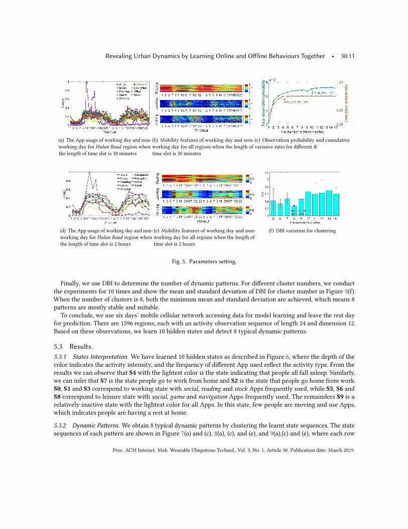
5.2 Experiments SettingIn order to determine the time granularity of our model, we compare the activity observations when usingdifferent length of time slot (i.e., 10 minutes, 20 minutes, 30 minutes, 1 hour, 2 hours, 3 hours, 4 hours). Whenthe length of time slot is shorter than 1 minutes, the observations of neighbor time slots are very similar. Butwhen the length of time slot is longer than 3 hours, the dynamics that the observation sequence reflects are toocoarse-grained. Thus, we show the parts of the observations of 30 minutes and 2 hours in Figure 5(a), (b), (d) and(e). Compare Figure 5(a) and (c), we can observe that the changing trend with time of App usage for differenttime granularity is consistent. Compare Figure 5(b) and (d), we can observe that peak and valley of mobility fordifferent time granularity also appear in the same time. Since the short one time slot is, the larger the number oftime slots is. Therefore, we set the length of the time slot as 2 hours as a trade-off between time granularity andmodel complexity.Then, to decide how many hidden states are suitable to present the characters of whole city, we analyze the

principal components of the mean vectors {µ1, µ2, ...µk , ..., µ20} of the Gaussian distribution and the probabilityof observation P(O |θ ) =

∏Rr=1 p(Or |θ ) for different number of hidden states. The cumulative variance ratio (CVR)

and P(O |θ ) with different number of states are shown in Figure 5(c) in red and blue, respectively. From theresults we can observe that when the number of hidden states is more 10, both the two curves converge to theirmaximum. Thus, we set K = 10 to learn states as different as possible at the lowest training cost.



(a) The App usage of working day and non-working day for Hulan Road region whenthe length of time slot is 30 minutes

(b) Mobility features of working day and non-working day for all regions when the length oftime slot is 30 minutes

(c) Observation probability and cumulativevariance ratio for different K

(d) The App usage of working day and non-working day for Hulan Road region whenthe length of time slot is 2 hours

(e) Mobility features of working day and non-working day for all regions when the length oftime slot is 2 hours

(f) DBI variation for clustering

Fig. 5. Parameters setting.

Finally, we use DBI to determine the number of dynamic patterns. For different cluster numbers, we conductthe experiments for 10 times and show the mean and standard deviation of DBI for cluster number in Figure 5(f).When the number of clusters is 8, both the minimum mean and standard deviation are achieved, which means 8patterns are mostly stable and suitable.

To conclude, we use six days’ mobile cellular network accessing data for model learning and leave the rest dayfor prediction. There are 1596 regions, each with an activity observation sequence of length 24 and dimension 12.Based on these observations, we learn 10 hidden states and detect 8 typical dynamic patterns.

5.3 Results.5.3.1 States Interpretation. We have learned 10 hidden states as described in Figure 6, where the depth of thecolor indicates the activity intensity, and the frequency of different App used reflect the activity type. From theresults we can observe that S4 with the lightest color is the state indicating that people all fall asleep. Similarly,we can infer that S7 is the state people go to work from home and S2 is the state that people go home from work.S0, S1 and S3 correspond to working state with social, reading and stock Apps frequently used, while S5, S6 andS8 correspond to leisure state with social, game and navigation Apps frequently used. The remainders S9 is arelatively inactive state with the lightest color for all Apps. In this state, few people are moving and use Apps,which indicates people are having a rest at home.

5.3.2 Dynamic Patterns. We obtain 8 typical dynamic patterns by clustering the learnt state sequences. The statesequences of each pattern are shown in Figure 7(a) and (c), 8(a), (c), and (e), and 9(a),(c) and (e), where each row



Fig. 6. The Gaussian mean of emission probability for each hidden state and the transition probabilities among these hiddenstates we obtain. Each state is shown in a column, 9 categories of Apps and 3 kinds of mobility are ranked in descendingorder by the mean value respectively, where the Bold denotes a value higher than 0.65, the Normal denotes a value higherthan 0.45 but no more than 0.65, and the Light denotes a value lower than 0.45.

(a) State sequences for pattern #1 (b) Mobility visualization for pattern #1

(c) State sequences for pattern #2 (d) Mobility visualization for pattern #2

Fig. 7. Visualization of state sequences and mobility for the residential, where the state sequence of each region is shownin a row on the left and the normalized mobility of each region is shown in a row on the right.

presents one region’s dynamics from the working day to the non-working day. The corresponding normalizedmobility S(Staying), L(Leaving) and A(Arriving) are shown in Figure 7(b) and (d), 8(b), (d) and (f), and 9(b), (d)and (f), respectively. We divide these 8 dynamic patterns into three classes to discuss their functions as follows:





(e) State sequences for pattern #5 (f) Mobility visualization for pattern #5

Fig. 8. Visualization of state sequences and mobility for the official, where the state sequence of each region is shown in arow on the left and the normalized mobility of each region is shown in a row on the right.

Residential regions: the first class shown in Figure 7 includes pattern #1 and #2. The common feature is thatS7 (in orange color) consistently appears at around 7am of the working day, which means people go to work fromhome at that time. From the three mobility features visualized in Figure 7(b) and (d), we can observe that lots ofpeople stay here before 7am, after 7pm of the working day, and in the whole non-working day. Besides, there areboth a leaving peak (in dark-red color) at around 7am and an arriving peak at around 7pm of the working daywhen people go to work and back to home, respectively. These characters give more indicators for the residentialregion. The difference between these two patterns is also obvious. S0 (in dark-blue color) and S1 (in navy-bluecolor) appear more frequently in pattern #2 than #1, which represents that a small group of people come toregions in pattern #2 and use stock Apps in the working day. From the mobility of pattern #2, we can also observethat there are an arriving peak at around 7am and a leaving peak at around 7pm. Thus, compared with pattern





(e) State sequences for pattern #8 (f) Mobility visualization for pattern #8

Fig. 9. Visualization of state sequences and mobility for the compound, where the state sequence of each region is shownin a row on the left and the normalized mobility of each region is shown in a row on the right.

#1, regions in pattern #2 mainly contain houses but also contain some office areas. In summary, pattern #1corresponds to single residence function, while pattern #2 corresponds mainly to residence but partly to officefunction.Official regions: the second class shown in Figure 8 including pattern #3, #4 and #5. The common feature is

that S4 and S5 (in green-series color) appear frequently during daytime in non-working day, which means fewpeople comes here in the weekend. The arriving peak at around 7am and the leaving peak at 7pm of workingday also support the interpretation of official areas. During daytime in weekday, S9 (in dark-red color) appearsfrequently in pattern #3, while S0 (in dark-blue color) and S1 (in navy-blue color) appear frequently in pattern #4and #5, representing that people work in the regions of pattern #3 use less Apps especially the stock Apps than inthe regions of pattern #4 and #5. Comparing pattern #4 and #5, we can observe that S7 (in orange color) also



appears at around 7 am when people leaving from home. Thus regions in pattern #5 mainly contain office butalso contain some residential areas. In summary, pattern #3 corresponds to single office function with few Appsused, pattern #4 corresponds to single office function with App used frequently, while pattern #5 correspondsmainly to office but partly to residence function.Compound regions: the third class shown in Figure 9 including pattern #6, #7 and #8 . The transition of

states is more complex than the first two classes. For pattern #6, S7 (in orange color) appears at anytime of thetwo days. The frequency of using Apps is rather stationary and people do not move intensively in a certaintime slot. Therefore, regions in pattern #6 are more likely to be far suburb with low population density. Forpattern #7 and #8, people are very active both in weekday and weekend. The ration of staying is consistently highboth in day and night, and people move frequently in the weekend. Thus these regions can be compound zonesperforming different functions in different time slots. Compared with pattern #8, S0 (in dark-blue color) and S1(in navy-blue color) in pattern #7 appear more frequently in working day. Besides, as shown in Figure 9(f), thenumber of people who move in and move out the regions in pattern #8 is always large at all time slot during theday. Therefore, pattern #7 covers the areas mainly playing the rule as office but also as houses and entertainmentsometime. Pattern #8 contains houses, entertainment areas, office as well as transportation hubs. In summary,pattern #6 corresponds to suburb function, pattern #7 corresponds mainly to office but partly to residence andentertainment function, while pattern #8 corresponds to highly dynamic and complex functions.In summary, these state sequences of the two typical days, reveal the regularity of human activities both in

terms of type and intensity. Different state sequences in the working time and non-working time also can indicatethe functions of a region. Consequently, we discover Pattern #1, #3, #4 and #6 with fundamental functions ofliving and working, and we also discover Pattern #2, #5, #7 and #8 with compound and dynamic functions.

5.4 Validations5.4.1 Validation with Check-ins. Check-ins reveal the purpose of user’s activity in the city intuitively. AlthoughPOIs are static, their popularity in different time slots would be various (e.g, restaurant POIs are most popular atnoon), and this dynamic popularity can be reflected by checked-in frequency. Therefore, we use check-ins tovalidate the detected dynamic patterns. Specifically, we explore the correlations between the state sequences andcheck-in POIs of each pattern. First, we merge the consecutive time slots under the same hidden state accordingto the center of each pattern. Then, we calculate the percentage of all kinds of POIs checked-in during the mergedtime slot. The results for three classes as mentioned in Section 5.3.2 are shown in Table 1, 2 and 3, respectively.In these tables, the Time row shows the time slot segmentation results, whereW denotes working day and Ndenotes non-working day, and the number afterW or N represents the hour of the day (e.g.,W 0-W 5 means fromworking day 0:00 to working day 5:59). The rest rows show the hidden state, the most frequently checked-in POIcategory, and the checked-in percentage in the corresponding time slots, respectively. The observations fromthese tables are as follows:

(1) From Table 1, we can observe that residence POIs are more popular in the sleeping hour (W 0-W 5, N 0-N 5)with the percentage of 37.8% in pattern #1 and 29.9% in patter #2, while transportation POIs are more popularduring rush hour (W 6-W 7, N 6-N 9) with the percentage exceeding 25% when people go to work. This indicatesthe dynamics that people rest in the night and go out in the morning, which is consist with the transition from S4to S7. Besides, during the daytime, people in pattern #1 are more likely to visit leisure POIs, while in pattern #2company and tourism POIs are more popular, which further proves that the function of pattern #2 changes fromresidence to office when the time changes from night to day. This also supports the existence of S0 in pattern #2.

(2) For the official regions as shown in Table 2, few people are active at night (W 0-W 7, N 0-N 9), which supportswhy S4 always appears at night. business and factory POIs are distinct in the working hour (W 10-W 17,W 8-W 15)with the percentage exceeding 20%, which means many people work here during the day as S1 indicates. It is



Table 1. Check-in POI components in different time slots for the residential, where POIs corresponding to their mainfunction are highlighted.

Pattern #1 Pattern #2

Time W0-W5 W6-W7 W8-W15 N10-N17 W0-W5 W6-W7 W8-W15 N8-N19N0-N5 N6-N9 N0-N5 N6-N9State S4 S7 S5 S8 S4 S7 S0 S8

Check-in POI Residence Transportation Leisure Leisure Residence Transportation Company TourismPercentage 37.8% 25.3% 28.7% 45.5% 29.9% 25.5% 18.4% 41.2%

Table 2. Check-in POI components in different time slots for the official, where POIs corresponding to their main functionare highlighted, and − denotes there are very few check-in records.

Pattern #3 Pattern #4 Pattern #5

Time W0-W9 W10-W17 N10-N17 W0-W7 W8-W15 N10-N17 W0-W5 W8-W15 N10-N17N0-N9 N0-N9 N0-N9State S4 S9 S4 S4 S1 S4 S4 S1 S5

Check-in POI - Factory Shopping - Business Tourism Residence Business TransportationPercentage - 21.3% 33.5% - 42.7% 25.6% 18.3% 20.1% 23.4%

Table 3. Check-in POI components in different time slots for the compound, where POIs corresponding to their mainfunction are highlighted, and − denotes there are very few check-in records.

Pattern #6 Pattern #7 Pattern #8

Time W0-W9 W10-W15 N10-N19 W0-W5 W8-W15 N10-N19 W0-W5 W8-W21 N10-N19N0-N9 W20-W21 N0-N7 N0-N7State S4 S9 S4 S4 S1 S9 S4 S9 S9

Check-in POI - Leisure Transportation Residence Business Tourism Transportation Transportation TourismPercentage - 19.1% 22.7% 15.6% 21.2% 20.1% 52.4% 15.6% 20.1%

worth noting that in pattern #5, the most popular POIs in the night is residence while in the day is office, whichshows that the function changes from residence to office. This is also consist with our previous analysis forpattern #5.

(3) For the compound regions as shown in Table 3, the most popular POIs are significantly different in differenttime slots, especially for pattern #7, which presents dynamic functions. Moreover, the percentage of transportationPOIs is generally high (i.e., more than 15%) in different time slots in pattern #8 , which indicates its high volumeof crowd flow. Interestingly, Disney Park and Hongqiao Airport are in this pattern, which all highly support theexistence of S9.

In summary, we analyze the POIs checked-in in different time slots for different patterns. All these results areconsistent with the semantic of learnt states and revealed dynamics.

5.4.2 Validation with Urban Land-use. In order to further verify the inferred functions, we compare them withthe urban land-use published by the local government. Figure 10(a) shows the land-use map including 6 type ofresidence, business, industry, public infrastructure, framing and forestry, and ecological restoration. From the resultwe can observe that Business areas (in red color) such as office buildings and residential areas (in creamy-whitecolor) are concentrated in the city centre, while outside are other functional areas. We also show the spatialdistribution of the eight dynamic patterns identified by our model in Figure 10(b), where each pattern is presented



in a unique color. Besides, the corresponding land-use types to our patterns as well as their functions are illustratedin Table 4. From Figure 10 and Table 4, we can observe that the most central working areas labeled by bluedash dot and the major living areas labeled by red dash-dot are well consistent between the land-use and ourpatterns. Besides, some regions with the large area are found to have the compound function, especially thePudong and Jinshan region, which is reasonable since such the land-use of such large regions cannot be single.Functions of each region are not available directly from the land-use plotting published by the government. Toquantitatively evaluate the dynamic patterns, we randomly select 100 regions of different patterns and manuallylabel their functions by checking their locations on the map. Finally, the functions of 81% of the selected regionsare consistent with our results, which further demonstrates the effectiveness of our revealed dynamics fromhuman activities.

(a) Urban land use (b) Dynamic patterns

Fig. 10. The spatial distribution for different regions in Shanghai, where within the polygon marked by blue dash dot isdowntown business area, outside the blue polygon but within the red polygon is downtown residence area, and the polygonlabeled by black dash dot denotes the most two coarse-grained regions Pudong and Jinshan.

Table 4. Relationship between land-use and our patterns.

Dynamic Patterns Pattern #1 Pattern #2 Pattern #3 Pattern #4&5 Pattern #6 Pattern #7&8Land-use / Region Residence Farming Industry Business Ecological Pudong, Jinshan, etc

Functions living living, working working working, living compound compound

5.5 Application of Prediction5.5.1 Tasks Design. Our proposed model can learn the patterns of human dynamic activities in different regionsin the city, which enable the prediction of people’s activities in next time slot. We design two prediction tasks asfollows:Crowd flow prediction: Given the mobility observation of a new day with the length of n time slots, we

predict how many people will move in, move out, or stay in (n + 1)-th time slot for each region.



Popular App prediction: Given the App usage observation of a new day with the length of n time slots, wepredict which Apps are used frequently in (n + 1)-th time slot for each region.As mentioned before, six days’ data are used for model training and the rest day’s data is used for prediction

evaluation. It is worth noting that testing data is pre-processed with the same normalization factors and sameparameters of the typical working as mentioned in section 3.1. Specially, for r -th region, we define the givenobservations as T = T1,T2, ...,TN , where Tr = Tr,1Tr,2...Tr,n(R = 1959, 1 ≤ n ≤ 11,L = 12). We also define thecandidate pool as all the observations in the training data. Then, our goal is to predict Tr,n+1 for region r at(n + 1)-th, which is determined by:

sr,n = argmax1≤j≤K

γ (s jr,n), (9)

sr,n+1 = argmax1≤k≤K

Aj,k , (10)

Tr,n+1 = argmaxr ′,1≤n′≤N

p(Or ′,n′ |sn+1 = k), (11)

where region r ′ and region r are in the same pattern [30]. We first use the current observations to determine theoptimal state sequence of these n time slots, and then to determine the next state by (9) and (10). The historyobservation with the maximum probability in (n + 1)-th state from the candidate pool is selected as the nextobservation by (11) [21]. Through anti-normalization, we obtain the number of crowd flows. By sorting theobservation of Apps, we obtain the most frequently used Apps.

5.5.2 Metrics and Baselines. To fully evaluate our system, we adopt three evaluation metrics: TopN-hitrate,TopN-accuracy and error ratio, which are defined in Appendix II. The first two metrics are used for popular appsprediction, among which TopN-hitrate is the percentage of regions whose TopN Apps are successfully predicted(i.e., correct for at least one), while TopN-accuracy reflects how many of the TopN Apps are predicted correctly.The last one is for crowd flows prediction, which is defined as the mean ratio of the difference between theprediction and the ground truth. As a comparison, we also conduct the prediction on our dataset by the followingthree baselines:HV : In this method, the prediction of (n + 1)-th time slot is theHistorical Value (HV) in the training data at thesame time slot (i.e., (n + 1)-th time slot in the typical working day) of the same region, directly [49].ARIMA: Aoto-Regression Integrated Moving Average (ARIMA) is a well-known model for time series analysisand prediction. We conduct the ARIMA prediction with the most suitable orders (i.e., suitable p, d and q) for eachregion [49].HMM: In order to show the ability of our model to deal with data sparsity, we train an independent HMM foreach region and conduct the prediction based on its own states instead of the shared ones [30].

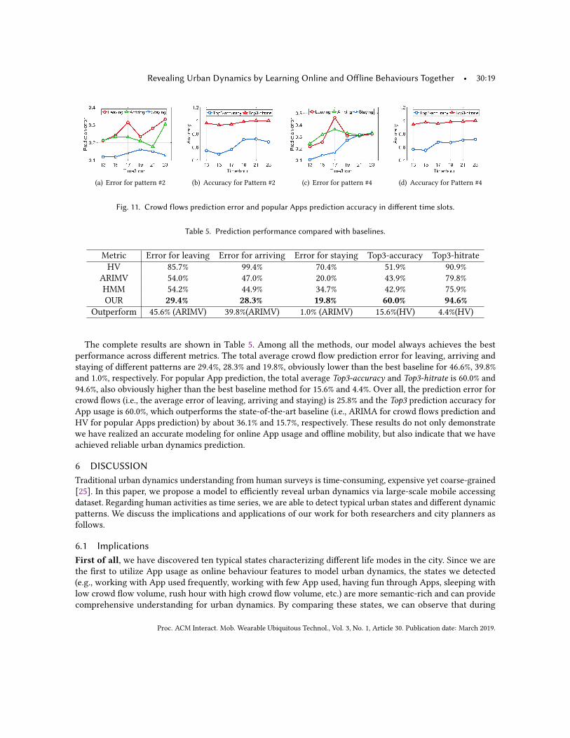
5.5.3 Results and Analysis. We evalute the performance of different regions with different length of givenobservations. First, we partly show the results for pattern #2 (a residential pattern) and #4 (an official pattern) inFigure 11. Over all, the prediction error is always lower than 50% and the accuracy is always higher than 50%.Specifically, from Figure 11(a) and (c), we can observe that the prediction for the number of people staying hereis more reliable than that of people moving in or moving out. The error of leaving and arriving prediction aremaximum at 11pm for pattern #2, while the staying prediction error are minimum at 11pm for pattern #4. Becausethere are usually few people in the official zones at night, thus the accuracy of the prediction would decline.Besides, about 5pm there is a rush hour in Friday, thus the prediction of mobility is not as correctly as usual.From Figure 11(b) and (d), we can observe that Top3-accuracy and Top3-hitrate is stable, where Top3-accuracyis always more than 50% and the Top3-hitrate is always more than 90% for all patterns in all time slots, whichdemonstrates our overall prediction accuracy is credible in different time slots.



(a) Error for pattern #2 (b) Accuracy for Pattern #2 (c) Error for pattern #4 (d) Accuracy for Pattern #4

Fig. 11. Crowd flows prediction error and popular Apps prediction accuracy in different time slots.

Table 5. Prediction performance compared with baselines.

Metric Error for leaving Error for arriving Error for staying Top3-accuracy Top3-hitrateHV 85.7% 99.4% 70.4% 51.9% 90.9%

ARIMV 54.0% 47.0% 20.0% 43.9% 79.8%HMM 54.2% 44.9% 34.7% 42.9% 75.9%OUR 29.4% 28.3% 19.8% 60.0% 94.6%

Outperform 45.6% (ARIMV) 39.8%(ARIMV) 1.0% (ARIMV) 15.6%(HV) 4.4%(HV)

The complete results are shown in Table 5. Among all the methods, our model always achieves the bestperformance across different metrics. The total average crowd flow prediction error for leaving, arriving andstaying of different patterns are 29.4%, 28.3% and 19.8%, obviously lower than the best baseline for 46.6%, 39.8%and 1.0%, respectively. For popular App prediction, the total average Top3-accuracy and Top3-hitrate is 60.0% and94.6%, also obviously higher than the best baseline method for 15.6% and 4.4%. Over all, the prediction error forcrowd flows (i.e., the average error of leaving, arriving and staying) is 25.8% and the Top3 prediction accuracy forApp usage is 60.0%, which outperforms the state-of-the-art baseline (i.e., ARIMA for crowd flows prediction andHV for popular Apps prediction) by about 36.1% and 15.7%, respectively. These results do not only demonstratewe have realized an accurate modeling for online App usage and offline mobility, but also indicate that we haveachieved reliable urban dynamics prediction.

6 DISCUSSIONTraditional urban dynamics understanding from human surveys is time-consuming, expensive yet coarse-grained[25]. In this paper, we propose a model to efficiently reveal urban dynamics via large-scale mobile accessingdataset. Regarding human activities as time series, we are able to detect typical urban states and different dynamicpatterns. We discuss the implications and applications of our work for both researchers and city planners asfollows.

6.1 ImplicationsFirst of all, we have discovered ten typical states characterizing different life modes in the city. Since we arethe first to utilize App usage as online behaviour features to model urban dynamics, the states we detected(e.g., working with App used frequently, working with few App used, having fun through Apps, sleeping withlow crowd flow volume, rush hour with high crowd flow volume, etc.) are more semantic-rich and can providecomprehensive understanding for urban dynamics. By comparing these states, we can observe that during



resting time, people keep on using social Apps while during working time, the most frequently used Apps areunexpectedly stock. We have also found eight dynamic patterns which are composed of these typical states.Second, compared with existing data-driven urban dynamics revealing systems [2, 24], our proposed state-sharingHMM can model the aggregated activities in a concise and probabilistic way, which means dynamic predictionis also achieved at the same time. Take pattern #2 as an example, as shown in Figure 11 (a) and (b), our modelcan predict the volume of arriving, leaving and staying as well as the popular Apps in the next time slot. Theprediction error is always less than 40% and the prediction accuracy is always higher than 50%. Based on ourprediction, city planners can make better urban management and resource allocation. Third, we demonstrate thaturban dynamics represented by online and offline behaviours can be used to infer urban functions. Compared withprevious urban function discovering works only using offline human mobility data and statistic POIs [43, 44, 53],we detect eight dynamic patterns corresponding to different functions. More importantly, we unexpectedly findthat among these dynamic patterns, some indicates single function such as pattern #1, which is simple residence,while the others indicate dynamic and compound functions such as pattern #2 and #5, which play the role asresidence and office alternately. All of these are our new contributions and make our findings significant.

6.2 ApplicationsOur work facilitates urban planning from different aspects. First and foremost, it provides more comprehensiveunderstanding for urban dynamics and urban functions. For architects, planners, and urban designers, neigh-borhood activity patterns from intensive ethnographic surveys that take years to conduct and given the speedat which neighborhoods change, can be out of date quickly. The features provided by our work helps examinethe diversity, distribution, and intensity of human activity within a given neighborhood, thus offering insightto the functioning of the entire neighborhood and supporting the government make better land use planning.Second, understanding and predicting the pattern of the crowd flow, the offline behaviours we utilize, is of greatsignificance for traffic dispatching, transportation infrastructure construction, etc. For example, according toour analysis, there is usually a leaving rush at 7-9am in the residence regions but an arriving rush at 8-10amin the office regions, which indicates different traffic demand in different regions and different time slots. Thisalso reminds the traffic management department to dynamically dispatch staffs and resources. Third, analyzingand predicting the App usage is also necessary for network operator to make better network infrastructureconstruction and resource allocation. For the regions with Apps used diversely and frequently, more base stationsand network resource are needed. Considering the dynamics of the usage of different App categories, a reasonableallocation strategy can improve the utilization of the existing network. In summary, our work sheds light on thefundamental dynamics in the city, which contributes to solving many urban issues.

6.3 LimitationsThis study is the first step to utilize the hidden Markov model to describe the urban dynamics. By sharing statesamong different regions, the difference, as well as similarities, could be learned around the city. Our work hasthe following limitations. First, the length of our data is one week, and we aggregate it to one working dayand one non-working day. Thus, we only exhibit the regular dynamics of working and non-working day. Weleave investigating more detailed daily, weekly and monthly dynamics as future work. Second, due to the datalimitation, we only evaluate the performance of prediction for the working day. References have demonstratedthat the most important time context for population [34, 39] as well as App usage [18, 36] prediction is the hourof the day and the day of the week. Therefore, one week’s data is enough for model evaluation [35, 37]. Theperformance of the baselines could be improved if more data are available. However, it would be limited, and ourmodel can still outperform the baselines as state-sharing strategy can make full use of the data and learn robustresults for urban dynamics.



7 CONCLUSIONIn this paper, we reveal urban dynamics by learning human online and offline behaviours together via a large-scaledataset of mobile cellular network accessing.We propose a state-sharingHMM system that models urban dynamicsand infers functions by extracting human activities of App usage and mobility. The evaluations demonstrate thatour system can effectively detect dynamic patterns. Our work opens a new angle to reveal urban dynamics usingonline and offline behaviours together, and paves the way for extensive applications including urban demandanalysis, land use planning, and activity prediction.

APPENDIX I: MODEL TRAININGThe specific process of the state-sharing HMM training and state sequence learning is described as below.

We use the Baum-Welch algorithm to train the model. Starting with random initial parameters, the EMalgorithm alternates between E-step and M-step round by round until the stop condition is satisfied. In the

(t + 1)-th round E-step, it computes the likehood functionQ(θ ,θ t ) =R∑r=1

∑Sp(S |Or ;θ t ) lnp(Or , S |θ ), and in M-step

it finds a new estimation θ (t+1) to maximizes the Q-function. The details of two steps are as follows:E-step: In this step, Q(θ t+1) based on the old parameter θ t in t-th round is computed. Given an observation

Or = Or,1Or,2...Or,n ...Or,N , the joint probability distribution over both hidden and observation variables is

p(Or , S |θ ) = p(sr,1 |π )N∑n=2

p(sr,n |sr,n−1,A)N∑

m=1p(Or,m |sr,m , µ,σ ). (12)

In order to compute the Q-function, the forward distribution α(sr,n) and backward distribution β(sr,n) aredefined as,

α(sr,n) = p(Or,1,Or,2, ...,Or,n , sr,n |θ(t )),

β(sr,n) = p(Or,n+1,Or,n+2, ...,Or,N , sr,n |θ(t )).

(13)

Here, α(sr,n) can be computed in a forward fashion, and β(sr,n) can be computed in a backward fashion:

α(sr,n) = p(Or,n |sr,n)∑sr ,n−1

α(sr,n−1)p(sr,n |sr,n−1),

β(sr,n) =∑sr ,n+1

β(sr,n+1)p(Or,n+1 |sr,n+1)p(sr,n+1 |sr,n),(14)

Obtaining the forward distribution α(sr,n) and backward distribution β(sr,n) , the other two probabilitiesof hidden states can be computed: (1)γ (sr,n = k), i.e., the probability of n-th hidden state to be k ; (2) ξ (sr,n =j, sr,n+1 = k), i.e., the probability of two consecutive states to be j and k . These two distributions are given by

γ (sr,n) = p(sr,n |Or ) = α(sr,n)β(sr,n)/p(Or ),

ξ (sr,n , sr,n+1) = p(sr,n1 , sr,n |Or ) = α(sr,n−1)p(sr,n |sr,n−1)P(Or,n |sr,n)β(sr,n)/p(Or ),(15)

where p(Or ) =∑

sr ,N α(sr,n).With the definitions of γ and ξ , the Q-function can be expressed from (12) as,

Q(θ ,θ t ) =R∑r=1

K∑k=1

γ (skr,1) lnπk +R∑r=1

N∑n=2

K∑j=1

K∑k=1

ξ (s jr,n−1, skr,n) lnAj,k +

R∑r=1

N∑n=1

K∑k=1

γ (skr,n) lnp(Or,n |µ,σ ), (16)

where skr,n is binary variable, and skr,n = 1 means the n-th hidden state is k . The whole training process is shownin Algorithm 1.



M-step: From (16), it’s interesting to see that the initial distribution π , the transition probabilities A and themean and variance of observation probability µ,σ are independent. Using Appropriate Lagrange multipliers, theparameters are easily to be achieved as follows:

π (t+1)k =

1R

R∑r=1

γ (skr,1),

A(t+1)j,k =

1Ξj

R∑r=1

N∑n=2

ξ (s jr,n−1, skr,n),

µ(t+1)k,l =1ΓK

R∑r=1

N∑n=1

γ (skr,n)or,n,l ,

σ (t+1)k,l =

1ΓK

R∑r=1

N∑n=1

γ (skr,n)(or,n,l − µ(t+1)k,l )2,

(17)

where ΓK =R∑r=1

N∑n=1

γ (skr,n), Ξj =R∑r=1

N∑n=2

K∑i=1

ξ (s jr,n−1, sir,n).

ALGORITHM 1: HMM training by EM algorithmInput: Observation dataset O = {O1,O2, ...,OR }(1 ≤ r ≤ R), Maximum IterationsMaxIter ;Output: HMM parameters θ = {π ,A, µ,σ };Procedure:

Initialization: t = 0, initial π (0)k = 1/K , A(0)

j,k = 1/K , µ(0)k,l = random(0, 1), σ (0)k,l = 0.01, ∀1 ≤ j,k ≤ K , 1 ≤ l ≤ L.

while t < MaxIter doE-step: Calculate α(sr,n )(t+1), β(sr,n )(t+1), γ (sr,n )(t+1), ξ (sr,n )(t+1), ∀1 ≤ r ≤ R, 1 ≤ n ≤ N utilizing old parametersθ (t ) by (14) - (15).

M-step: Update π (t+1)k , A(t+1)

j,k , µ(t+1)k,l , σ (t+1)k,l , ∀1 ≤ j,k ≤ K , 1 ≤ l ≤ L utilizing γ (sr,n )(t+1), ξ (sr,n )(t+1) by (17).

Update t : t = t + 1end

APPENDIX II: EVALUATION METRICSFor each region r in each time slot n int the test set, we denote the truth app usage X (r ,n, l)(1 ≤ l ≤ La) as avectorUr,n and the corresponding prediction vector asU pre

r,n . We also denote the truth population as Lr,n , Ar,n

and Sr,n and the corresponding prediction as Lprer,n , Aprer,n and Sprer,n . Then the TopN-hitrate, TopN-accuracy and runs

as follows:

TopN − hitrate =

(∑r

(|Ur,n ∩U

prer,n | ≥ 1

))/R, (18)

TopN − accuracy =

(∑r

|Ur,n ∩Uprer,n |

N

)/R, (19)

Error f or leavinд =

(∑r

|Lprer,n − Lr,n |

Lr,n

)/R, (20)



where the error for arriving and staying is the same with the formula for leaving.

REFERENCES[1] 2018. Mobile Marketing Statistics compilation. https://www.smartinsights.com/mobile-marketing/mobile-marketing-analytics/

mobile-marketing-statistics/. (2018).[2] Sofiane Abbar, Tahar Zanouda, Noora Al-Emadi, and Rachida Zegour. 2018. City of the People, for the People: Sensing Urban Dynamics

via Social Media Interactions. In Social Informatics, Steffen Staab, Olessia Koltsova, and Dmitry I. Ignatov (Eds.). Springer InternationalPublishing, Cham, 3–14.

[3] J. R. Bellegarda and D. Nahamoo. 1990. Tied mixture continuous parameter modeling for speech recognition. IEEE Transactions onAcoustics, Speech, and Signal Processing 38, 12 (Dec 1990), 2033–2045.

[4] M. Bishop Christopher. 2016. PATTERN RECOGNITION AND MACHINE LEARNING. In Springer-Verlag New York. 605–652.[5] Demissie M D, Correia G, and Bento C. 2015. Analysis of the pattern and intensity of urban activities through aggregate cellphone

usage. Transportmetrica A: Transport Science 11, 6 (2015), 502–524.[6] D. L. Davies and D. W. Bouldin. 1979. A Cluster Separation Measure. IEEE Transactions on Pattern Analysis and Machine Intelligence

PAMI-1, 2 (April 1979), 224–227.[7] Adriana de Souza e Silva. 2006. From Cyber to Hybrid: Mobile Technologies as Interfaces of Hybrid Spaces. Space and Culture 9, 3

(2006), 261–278.[8] Riccardo Di Clemente, Miguel Luengo-Oroz, Matias Travizano, Sharon Xu, Bapu Vaitla, and Marta C González. 2018. Sequences of

purchases in credit card data reveal lifestyles in urban populations. Nature communications 9 (2018).[9] Manuel GarcÃŋa Docampo. 2014. Theories of Urban Dynamics. In International Journal of Population Research, Vol. 2014.[10] Jacques Gabarro-Arpa and Roger Revilla. 2000. Clustering of a molecular dynamics trajectory with a Hamming distance. Computers &

Chemistry 24, 6 (2000), 693 – 698.[11] Marta C. GonzÃąlez, CÃľsar A. Hidalgo, and Albert-LÃąszlÃş BarabÃąsi. 2008. Understanding individual human mobility patterns.

Nature 453, 7196 (2008), 779–783.[12] Xuedong Huang, Fileno Alleva, Hsiao-Wuen Hon, Mei-Yuh Hwang, Kai-Fu Lee, and Ronald Rosenfeld. 1993. The SPHINX-II speech

recognition system: an overview. Computer Speech & Language 7, 2 (1993), 137 – 148.[13] X. D. Huang. 1992. Phoneme classification using semicontinuous hidden Markov models. IEEE Transactions on Signal Processing 40, 5

(May 1992), 1062–1067.[14] Mei-Yuh Hwang and Xuedong Huang. 1993. Shared-Distribution Hidden Markov Models for Speech Recognition. 1 (11 1993), 414 – 420.[15] Maxime Lenormand, Miguel Picornell, Oliva G Cantú-Ros, Thomas Louail, Ricardo Herranz, Marc Barthelemy, Enrique Frías-Martínez,

Maxi San Miguel, and José J Ramasco. 2015. Comparing and modelling land use organization in cities. Royal Society open science 2, 12(2015), 150449.

[16] Maxime Lenormand and José J Ramasco. 2016. Towards a better understanding of cities using mobility data. Built Environment 42, 3(2016), 356–364.

[17] Kenneth Rose Liang Gu, Jayanth Nayak. 2000. Discriminative training of tied-mixture HMM by deterministic annealing. ICSLP-2000 4(2000).

[18] Zhung-Xun Liao, Yi-Chin Pan, Wen-Chih Peng, and Po-Ruey Lei. 2013. On Mining Mobile Apps Usage Behavior for Predicting AppsUsage in Smartphones. In Proceedings of the 22Nd ACM International Conference on Information & Knowledge Management (CIKM ’13).ACM, New York, NY, USA, 609–618.

[19] Thomas Louail, Maxime Lenormand, Miguel Picornell, Oliva García Cantú, Ricardo Herranz, Enrique Frias-Martinez, José J Ramasco,and Marc Barthelemy. 2015. Uncovering the spatial structure of mobility networks. Nature Communications 6 (2015), 6007.

[20] Thomas Louail, Maxime Lenormand, Oliva G Cantu Ros, Miguel Picornell, Ricardo Herranz, Enrique Frias-Martinez, José J Ramasco,and Marc Barthelemy. 2014. From mobile phone data to the spatial structure of cities. Scientific reports 4 (2014), 5276.

[21] Q. Lv, Y. Qiao, N. Ansari, J. Liu, and J. Yang. 2017. Big Data Driven Hidden Markov Model Based Individual Mobility Prediction at Pointsof Interest. IEEE Transactions on Vehicular Technology 66, 6 (June 2017), 5204–5216.

[22] Ping Wang Marcus Berliant. 2015. Dynamic Urban Models: Agglomeration and Growth. In Urban Dynamics and Growth: Advances inUrban Economics (Mar 2015), 533–581.

[23] Wesley Mathew, Ruben Raposo, and Bruno Martins. 2012. Predicting future locations with hidden Markov models. In Proceedings of the2012 ACM conference on ubiquitous computing. ACM, 911–918.

[24] F. Miranda, H. Doraiswamy, M. Lage, K. Zhao, B. GonÃğalves, L. Wilson, M. Hsieh, and C. T. Silva. 2017. Urban Pulse: Capturing theRhythm of Cities. IEEE Transactions on Visualization and Computer Graphics 23, 1 (Jan 2017), 791–800.

[25] JEFFREY D. MORENOFF, ROBERT J. SAMPSON, and STEPHEN W. RAUDENBUSH. [n. d.]. NEIGHBORHOOD INEQUALITY, COLLEC-TIVE EFFICACY, AND THE SPATIAL DYNAMICS OF URBAN VIOLENCE*. Criminology 39, 3 ([n. d.]), 517–558.


https://www.smartinsights.com/mobile-marketing/mobile-marketing-analytics/mobile-marketing-statistics/

https://www.smartinsights.com/mobile-marketing/mobile-marketing-analytics/mobile-marketing-statistics/


[26] FlÃąvio Nunes. 2006. The Portuguese urban system: An opposition between its hierarchical organization in cyberspace vs. physicalspace. Telematics and Informatics 23, 2 (2006), 74 – 94.

[27] Jiaul H. Paik. 2013. A Novel TF-IDF Weighting Scheme for Effective Ranking. In Proceedings of the 36th International ACM SIGIRConference on Research and Development in Information Retrieval (SIGIR ’13). ACM, New York, NY, USA, 343–352.

[28] Bryan C Pijanowski, Daniel G Brown, Bradley A Shellito, and Gaurav A Manik. 2002. Using neural networks and GIS to forecast landuse changes: a Land Transformation Model. Computers, Environment and Urban Systems 26, 6 (2002), 553 – 575.

[29] L. R. Rabiner. 1989. A tutorial on hidden Markov models and selected applications in speech recognition. Proc. IEEE 77, 2 (Feb 1989),257–286.

[30] Hongbo Si, Yue Wang, Jian Yuan, and Xiuming Shan. 2010. Mobility Prediction in Cellular Network Using Hidden Markov Model. (022010), 5 pages.

[31] Jameson L. Toole, Michael Ulm, Marta C. González, and Dietmar Bauer. 2012. Inferring Land Use from Mobile Phone Activity. InProceedings of the ACM SIGKDD International Workshop on Urban Computing (UrbComp ’12). ACM, New York, NY, USA, 1–8.

[32] Zhen Tu, Runtong Li, Yong Li, Gang Wang, Di Wu, Pan Hui, Li Su, and Depeng Jin. 2018. Your Apps Give You Away: DistinguishingMobile Users by Their App Usage Fingerprints. Proc. ACM Interact. Mob. Wearable Ubiquitous Technol. 2, 3, Article 138 (Sept. 2018),23 pages.

[33] ANDREW J. VITERBI. [n. d.]. Error Bounds for Convolutional Codes and an Asymptotically Optimum Decoding Algorithm. 41–50.[34] Huandong Wang, Fengli Xu, Yong Li, Pengyu Zhang, and Depeng Jin. 2015. Understanding Mobile Traffic Patterns of Large Scale

Cellular Towers in Urban Environment. In Proceedings of the 2015 ACM Internet Measurement Conference, IMC 2015, Tokyo, Japan, October28-30, 2015. 225–238.

[35] Jing Wu, Ming Zeng, Xinlei Chen, Yong Li, and Depeng Jin. 2018. Characterizing and Predicting Individual Traffic Usage of MobileApplication in Cellular Network. In Proceedings of the 2018 ACM International Joint Conference and 2018 International Symposium onPervasive and Ubiquitous Computing and Wearable Computers. ACM, 852–861.

[36] Fengli Xu, Yong Li, Min Chen, and Sheng Chen. 2016. Mobile cellular big data: linking cyberspace and the physical world with socialecology. IEEE Network 30, 3 (2016), 6–12.

[37] Fengli Xu, Yu-Yun Lin, Jiaxin Huang, Di Wu, Hongzhi Shi, Jeungeun Song, and Yong Li. 2016. Big Data Driven Mobile TrafficUnderstanding and Forecasting: A Time Series Approach. IEEE Trans. Services Computing 9, 5 (2016), 796–805.

[38] Fengli Xu, Tong Xia, Hancheng Cao, Yong Li, Funing Sun, and Fanchao Meng. 2018. Detecting Popular Temporal Modes in Population-scale Unlabelled Trajectory Data. Proc. ACM Interact. Mob. Wearable Ubiquitous Technol. 2, 1, Article 46 (March 2018), 25 pages.

[39] Fengli Xu, Pengyu Zhang, and Yong Li. 2016. Context-aware real-time population estimation for metropolis. In Proceedings of the 2016ACM International Joint Conference on Pervasive and Ubiquitous Computing, UbiComp 2016, Heidelberg, Germany, September 12-16, 2016.1064–1075.

[40] Hongyi Yao, Gyan Ranjan, Alok Tongaonkar, Yong Liao, and Zhuoqing Morley Mao. 2015. SAMPLES: Self Adaptive Mining of PersistentLExical Snippets for ClassifyingMobile Application Traffic. In Proceedings of the 21st Annual International Conference on Mobile Computingand Networking (MobiCom ’15). ACM, New York, NY, USA, 439–451.

[41] Donghan Yu, Yong Li, Fengli Xu, Pengyu Zhang, and Vassilis Kostakos. 2018. Smartphone App Usage Prediction Using Points of Interest.Proc. ACM Interact. Mob. Wearable Ubiquitous Technol. 1, 4, Article 174 (Jan. 2018), 21 pages.

[42] Jing Yuan, Yu Zheng, and Xing Xie. 2012. Discovering Regions of Different Functions in a City Using Human Mobility and POIs. InProceedings of the 18th ACM SIGKDD International Conference on Knowledge Discovery and Data Mining (KDD ’12). ACM, New York, NY,USA, 186–194.

[43] N. J. Yuan, Y. Zheng, X. Xie, Y. Wang, K. Zheng, and H. Xiong. 2015. Discovering Urban Functional Zones Using Latent ActivityTrajectories. IEEE Transactions on Knowledge and Data Engineering 27, 3 (March 2015), 712–725.

[44] N. J. Yuan, Y. Zheng, X. Xie, Y. Wang, K. Zheng, and H. Xiong. 2015. Discovering Urban Functional Zones Using Latent ActivityTrajectories. IEEE Transactions on Knowledge and Data Engineering 27, 3 (March 2015), 712–725.

[45] Chao Zhang, Keyang Zhang, Quan Yuan, Haoruo Peng, Yu Zheng, Tim Hanratty, Shaowen Wang, and Jiawei Han. 2017. Regions,Periods, Activities: Uncovering Urban Dynamics via Cross-Modal Representation Learning. In Proceedings of the 26th InternationalConference on World Wide Web (WWW ’17). International World Wide Web Conferences Steering Committee, Republic and Canton ofGeneva, Switzerland, 361–370.

[46] Chao Zhang, Keyang Zhang, Quan Yuan, Fangbo Tao, Luming Zhang, Tim Hanratty, and Jiawei Han. 2017. React: Online multimodalembedding for recency-aware spatiotemporal activity modeling. In Proceedings of the 40th International ACM SIGIR Conference onResearch and Development in Information Retrieval. ACM, 245–254.

[47] Chao Zhang, Keyang Zhang, Quan Yuan, Luming Zhang, Tim Hanratty, and Jiawei Han. 2016. GMove: Group-Level Mobility ModelingUsing Geo-Tagged Social Media. In Proceedings of the 22Nd ACM SIGKDD International Conference on Knowledge Discovery and DataMining (KDD ’16). ACM, New York, NY, USA, 1305–1314.

[48] Ke Zhang, Qiuye Jin, Konstantinos Pelechrinis, and Theodoros Lappas. 2013. On the Importance of Temporal Dynamics in ModelingUrban Activity. In Proceedings of the 2Nd ACM SIGKDD International Workshop on Urban Computing (UrbComp ’13). ACM, New York,



NY, USA, Article 7, 8 pages.[49] Yu Zheng Zhang, Junbo and Dekang Qi. 2017. Deep Spatio-Temporal Residual Networks for Citywide Crowd Flows Prediction. In AAAI.

1655–1661.[50] Yu Zheng, Licia Capra, Ouri Wolfson, and Hai Yang. 2014. Urban Computing: Concepts, Methodologies, and Applications. ACM Trans.

Intell. Syst. Technol. 5, 3, Article 38 (Sept. 2014), 55 pages.[51] M. Zhou, M. Wang, and Q. Hu. 2013. A POI data update approach based on Weibo check-in data. In 2013 21st International Conference on

Geoinformatics. 1–4.[52] Wanzheng Zhu, Chao Zhang, Shuochao Yao, Xiaobin Gao, and Jiawei Han. 2018. A Spherical Hidden Markov Model for Semantics-Rich

Human Mobility Modeling.. In AAAI.[53] Bin Liu Wangsu Hu Hui Xiong Zijun Yao, Yanjie Fu. 2018. Representing Urban Functions through Zone Embedding with Human

Mobility Patterns. In Proceedings of the Twenty-Seventh International Joint Conference on Artificial Intelligence (IJCAI-18).

Received August 2018; revised October 2018; accepted January 2019


Documents

Revealing Urban Dynamics by Learning Online and Offline