Revealed Attention∗

Yusufcan Masatlioglu Daisuke Nakajima Erkut Y. Ozbay

December 2010

Abstract

The standard revealed preference argument relies on an implicit assumption

that a decision maker considers all feasible alternatives. However, the market-

ing and psychology literatures provide well-established evidence that consumers

do not consider all brands in a given market before making a purchase (Limited

Attention). In this paper, we illustrate how one can deduce both the decision

maker’s preference and the alternatives to which she pays attention and inat-

tention from the observed behavior. We illustrate how seemingly compelling

welfare judgements without specifying the underlying choice procedure are mis-

leading. Further, we provide a choice theoretical foundation for maximizing a

single preference relation under limited attention.

JEL Classification: D11, D81.

Keywords: Revealed Preferences, Awareness, Attention, Consideration Set

∗We would like to thank Tilman Borgers, Emel Filiz-Ozbay, Stephan Lauermann, Paola Manzini,Marco Mariotti, Collin Raymond and Neslihan Uler for their helpful comments. Yusufcan Masatli-oglu and Daisuke Nakajima thank the National Science Foundation for financial support under GrantSES-1024544.

1

1 Introduction

Revealed preference is one of the most influential ideas in economics and has been

applied to a number of areas of economics, including consumer theory.1 According to

the standard revealed preference theory, x is revealed to be preferred to y if and only if

x is chosen when y is also available (Paul A. Samuelson (1938)). Any choice reversal,

therefore, observed both empirically and experimentally, is attributed to irrationality

since it cannot be expressed as a preference maximization.

The revealed preference argument relies on the implicit assumption that a deci-

sion maker (DM) considers all feasible alternatives. Without the full consideration

assumption, the standard revealed preference method can be misleading. It is possi-

ble that the DM prefers x to y but she chooses y when x is present simply because

she does not realize that x is also available (Daniel Hausman (2008)). For example,

while using a search engine, a DM might only pay attention to alternatives appear-

ing on the first page of the results since it takes too much time to consider all the

search results. She then picks the best alternative of those on the first page, say

y. It is possible that her most preferred item, x, does not appear in the first page.

Therefore we, as outside observers, cannot conclude y is better than x even though

y is chosen when x is available. Nevertheless, as in the above example, the DM may

have a well-defined preference and is maximizing her preference within her bounded

understanding of what is available.2

This immediately raises a question: How can we elicit her (stable) preference

without the full attention assumption? We consider a DM who picks her most pre-

ferred item from the alternatives she pays attention to, not from the entire feasible

set. Then we shall illustrate when and how one can deduce both the DM’s preferences

and the alternatives to which she does or does not pay attention from her observed

choices. Furthermore, we illustrate the problem of the welfare judgement without

specifying the underlying choice procedure by showing an example where our method

and the conservative criterion of Douglas B. Bernheim and Antonio Rangel (2007,

1Hal R. Varian (2006) provides a nice survey of revealed preference analysis.2As argued in Robert J. Aumann (2005), this behavior is still considered rational (at least bound-

edly rational) since she is choosing the best alternative under her limited information of what isavailable.

1

2009) result in the completely opposite implication.

The marketing literature calls the set of alternatives to which a DM pays attention

in her choice process as the consideration set (Peter Wright and Fredrick Barbour

(1977)). The formation of the consideration set has been extensively studied in mar-

keting and finance literatures (e.g. John R. Hauser and Birger Wernerfelt (1990);

John H. Roberts and James M. Lattin (1991)). It has been argued that due to cog-

nitive limitations, DMs cannot pay attention to all the available alternatives. As

Herbert A. Simon (1957) pointed out, being able to consider all possible alternatives

is as hard as comparing them for decision makers. Therefore, a DM with limited cog-

nitive capacity (possibly stemming from unawareness as demonstrated in Michelle S.

Goeree (2008)3) , restricts her attention only to a small fraction of the objects present

in the associated market (George J. Stigler (1961), Edgar A. Pessemier (1978), Jeong-

wen, Chiang, Siddhartha Chib and Chakravarthi Narasimhan (1998).4 In sum, DMs

intentionally or unintentionally filter out some alternatives to prevent her cognitive

capacity from being overloaded (Donald E. Broadbent (1958)).

The common property in the formation of consideration sets is that it is unaffected

when an alternative she does not pay attention to becomes unavailable. This basic

property of the attention filter, which is also documented in the psychology literature

(Broadbent (1958)), can be interpreted as the minimal condition. This property is

trivially satisfied in the classical choice theory where it is assumed that the DM is

able to pay attention to all the available alternatives. Additionally, it is normatively

appealing especially when a DM pays attention to all of items she is aware of and is

unaware that she is unaware of other items. For example, if a PC buyer is not only

unaware of a particular PC, but she is also unaware that she overlooks that PC, then,

even when that PC becomes unavailable, such a change will not be recognized by her.

Therefore, her consideration set will stay the same.

3Robert J. Lavidge and Gary A. Steiner (1961) presented awareness of an item as a necessarycondition to be in the consideration set. How unawareness alters the behavior of the DM has beenstudied in various contexts such as game theory (Aviad Heifetz, Martin Meier and Burkhard C.Schipper(2010), Erkut Y. Ozbay (2008)), and contract theory (Emel Filiz-Ozbay (2010)).

4In addition, in financial economics it is shown that investors reach a decision within their limitedattention (Gur Huberman and Tomer Regev (2001)). Similar examples can be found in job search(Max D. Richards, John E. Sheridan and John W. Slocum (1975)), university choice (Philip L.Dawes and Jennifer Brown (2005)), and airport choice (Gozen Basar and Chandra Bhat (2004)).

2

Interestingly, the property is also satisfied when the DM actually chooses the

consideration sets by taking the cost of investigation and the expected benefit into

account. Suppose the DM excludes x from her consideration. If x becomes unavail-

able, she has no reason to add or remove any alternative to her consideration set

because she could have done so when x was available. Therefore, her consideration

set is not affected when x becomes unavailable. Furthermore, this property is also

satisfied when the formation is based on many decision heuristics, such as paying

attention only to the N-most advertised alternatives or the products appearing in the

first page of search results. As a result, our property is appealing from both normative

and descriptive point of views.

In this paper, we refer to the consideration sets satisfying this property as attention

filters. Under this structure, it is possible to elicit the DM’s preference whenever a

choice reversal is observed.5 For example, assume that she chooses x but removing y

changes the choice. This can happen only when her consideration set has changed.

This would be impossible if she did not pay attention to y. Hence, y must have

been considered (Revealed Attention). Given the fact that x is chosen while y draws

her attention, we conclude that she prefers x over y (Revealed Preference). In sum,

whenever her choices changes as a consequence of removing an unchosen alternative,

the initially chosen alternative is preferred to the removed one.

Given that our identification strategy relies on the particular choice procedure,

where she maximizes her preference within her attention filter, it is natural to ask

the falsifiability of our model. We show that our model is fully characterized by

weakening the Weak Axiom of the Revealed Preference (WARP). This result renders

our model behaviorally testable.

Our method to distinguish between a preference and attention/inattention gener-

ates several policy implications. For instance, if a product of a firm is unpopular in

the market place, there could be two different explanations: (i) the product has a low

evaluation by consumers or (ii) it does not attract attention of consumers. Identifying

the right reason will lead to different strategies for the firm to improve the sales.

Our paper also contributes to the recent discussion about welfare analysis under

5Without any structure on the formation of the consideration sets, any choice behavior can berationalized by any preference (Hausman (2008)).

3

non-standard individual behavior.6 We elicit the DM’s preference in a positive ap-

proach, which is based on a particular choice procedure. Bernheim and Rangel (2009)

criticize such an approach by arguing that it is not necessary to explain the behavior

to make a welfare analysis. Instead, they make welfare arguments directly from the

choice data without assuming any choice procedure (model-free). Particularly, they

claim that y is strictly welfare improving over x if y is sometimes chosen when x is

available but x is never chosen when y is present. However, this intuitive criteria of

welfare analysis is meaningful only if the DM considers all the presented alternatives.7

In Section 3, we discuss this issue in detail to illustrate the problem of the naive use

of the model-free approach. Indeed, we provide an example where their welfare im-

plication contradicts our revealed preference (hence the actual preference); that is, y

is revealed to be preferred to x even when x is strictly welfare improving over y in

Bernheim and Rangel (2009)’s sense.

So far we have discussed how one can elicit DM’s preference and consideration sets

in our model. In doing so, we impose a relatively weak condition on the formation of

consideration sets so that our approach is applicable to a wide range of choice data.

As a result, although our model is refutable, it provides an alternative explanation

for several frequently observed behaviors that cannot be captured by the standard

choice theory: Attraction Effect, Cyclical Choice, and Choosing Pairwisely Unchosen

(see Anomalies section). Our explanations for these choice patterns solely depend on

limited attention, hence seemingly irrational behaviors can be explained without in-

troducing changing preference. Nevertheless, depending on the intended application,

it is possible to analyze this framework under different restrictions on consideration

sets (see Concluding Remarks).

There are several related models where the final choice is made after eliminat-

ing several items, which can be interpreted as a choice with limited consideration

such as applying a rationale to eliminate alternatives (Manzini and Mariotti (2007),

6See Attila Ambrus and Kareen Rozen (2010), Jose Apesteguia and Miguel A. Ballester (2010),Vadim Cherepanov, Timothy Feddersen and Alvaro Sandroni (2010), Christopher P. Chambers andTakashi Hayashi (2008), Paola Manzini and Marco Mariotti (forthcoming), Yusufcan Masatlioglu andDaisuke Nakajima (2007), Jawad Noor (forthcoming), Ariel Rubinstein and Yuval Salant (2010)).

7Indeed, Bernheim and Rangel (2007) mention that if we know the DM believes that she ischoosing from a set that is other than the objective feasible set, we should take it into account forthe welfare analysis (Section III B).

4

Apesteguia and Ballester (2008), Nicolas Houy (2007), Houy and Koichi Tadenuma

(2009)), focusing only on alternatives a decision maker can rationalizes to choose

by some other criteria (Cherepanov, Feddersen and Sandroni (2010)) and consid-

ering only alternatives belonging to undominated categories (Manzini and Mariotti

(forthcoming)). Our model is both descriptively and behaviorally distinct from these

models. In addition, unlike our model, these models implicitly assume that a DM

considers all feasible alternatives at the first stage and intentionally eliminates several

alternatives. Therefore, their stories are not applicable to cases where the source of

limited consideration is unawareness of some alternatives.

Finally, we would like to compare several other models involving consideration

sets in decision theory. Juan S. Lleras, et al. (2010) study a different model of choice

under limited consideration where a product attracting attention in a crowded su-

permarket shelf will be noticed when there are fewer products. While this paper is

complementary to our paper, their implications are completely different (see Conclud-

ing Remarks for more discussion). Masatlioglu and Nakajima (2009) propose a model

of an iterative search where a decision maker cannot consider all alternatives, which

can be because of unawareness like our model. The difference is that they emphasize

that a consideration set depends on the initial starting point and evolves dynamically

during the course of search. In the models of Andrew Caplin and Mark Dean (forth-

coming) and Caplin, Dean and Daniel Martin (forthcoming), a decision maker goes

through alternative sequentially and, at any given time, chooses the best one among

those she has searched. Unlike our model, their “choice process” data includes not

only the DM’s choice without time limit, but also what she would choose if she were

suddenly forced to quit the search at any given time.

Kfir Eliaz and Ran Spiegler (forthcoming) analyze a market where firms would like

to manipulate consumers’ consideration sets by using costly marketing devices. Eliaz,

Michael Richter and Rubinstein (forthcoming) study a very concrete and reasonable

way to construct a consideration set. Indeed, some of consideration sets we shall

present as examples are within their models. However, contrary to our model, in

their paper, the decision maker’s consideration set (called finalists) is observed and

is directly investigated. In our model the consideration set is an object that must be

inferred from the DM’s final choice.

5

The outline of this paper is as follows: Section 2 introduces the basic notations and

definitions. In Section 3, we provide two characterization for the revealed preference

and the revealed (in)attention from observed choice data. Section 4 provides a simple

behavioral test for our model and discusses the related literature. Then, in Section

5, we illustrate that our limited attention model is capable of accommodating several

frequently observed behaviors. Finally the Further Comments and the Concluding

Remarks sections conclude the paper.

2 The Model

Throughout this paper, let X be a finite set of alternatives that may be available for

a decision maker to choose. X denotes the set of all non-empty subsets of X, which

is interpreted as the collection of all the (objective) feasible sets observed by a third

party.

2.1 Attention Filters

In our model, a decision maker picks the best element from those she pays attention

to. Our goal is to elicit her preference along with her attention and inattention from

her actual choice data. However,this is impossible without any knowledge about her

attention and inattention. One can always claim that she picks an alternative because

she ignores everything else so one cannot infer her preference at all.

We now propose a property how consideration sets change as feasible sets change,

instead of explicitly modeling how the feasible set determines the consideration set.

This approach makes it possible to apply our method to elicit the preference without

relying on a particular formation of the consideration set. We shall explain that this

property is normatively compelling in several situations and is indeed true in many

heuristics people actually use in the real life.

Let S be a feasible set the decision maker is facing. She does not pay attention

to all alternatives in S. Let Γ(S) be the (non-empty) set of elements to which she

pays attention. Formally, Γ is a mapping from X to X with ∅ 6= Γ(S) ⊂ S. We call

it a consideration set mapping. Of all consideration set mappings, we focus on those

6

having the following property:

Definition 1. A consideration set mapping Γ is an attention filter if for any S,

Γ(S) = Γ(S \ x) whenever x 6∈ Γ(S).8

This definition says that if an alternative does not attract an attention of the

decision maker, her consideration set does not change when such an item becomes

unavailable.

To illustrate that this is a normatively appealing property, we shall provide two

examples where the decision maker’s consideration set mapping should be an attention

filter. The first example is based on unawareness. Imagine a decision maker (wrongly)

believes Γ(S) is her feasible set (S is the actual one). That is, she is not only unaware

of alternatives in S \Γ(S) and but unaware that she is unaware of these alternatives.

If so, she will not recognize the change of the feasible set when such an item becomes

unavailable so her consideration set should not change. This is exactly what the

property dictates.

The second one is choosing rationally what to consider (or not to consider). Be-

cause of scarcity of time and/or complexity of decision problems, a decision maker

selectively focuses on a smaller set of alternatives and ignores the rest. Suppose

she knows S is her entire feasible set. Then, she picks her consideration set Γ(S)

optimally based on her prior beliefs about the value of alternatives and the cost of

inspecting them. Then, her consideration set mapping must satisfy our property. To

see this, imagine that she considers only a and b when her feasible set is {a, b, c, d}(Γ({a, b, c, d}) = {a, b}). Assume that d becomes unavailable now. She has no reason

to add c to her consideration set because she could have done so when d was available.

For the same reason, it is not rational to remove b (or a) from her consideration set.

Therefore, it must be Γ({a, b, c}) = {a, b}. That is, her consideration set mapping is

an attention filter. Notice that this must be true whatever beliefs and cost function

she has.9

Furthermore, in addition to being normatively appealing, our condition is also

descriptively appealing. Many heuristics that are actually used to narrow down the

8Throughout the paper, we write S \ x instead of S \ {x} for simplicity.9The only exception is that the feasible set itself conveys some information that affects her belief

or cost function.

7

set of choosable options generate attention filters. We list some of them.

. Top N: A decision maker considers only top N alternatives according to some

criterion that is different from her preference. For instance:

• Consider only the three cheapest suppliers in the market (Uwe Dulleck, et al

(2008)).

• Consider the N most advertised products in the market.

• Consider the products that appear in the first page of the websearch and/or

sponsored links (Gord Hotchkiss, et al (2004)).

• Consider the first N available alternatives according to an exogenously given

order (Salant and Rubinstein (2008)).10

. Top on each criterion: A decision maker has several criteria and considers

only the best alternative(s) in each criterion.11 For instance:

• Consider only a job candidate if she the best in a program. Or consider the

top two job candidates from all first-tier schools and the top candidate from

second-tier schools.

• Consider only the cheapest car, the safest car, and the most fuel efficient car in

the market.

. Most popular category: A decision maker considers alternatives that belong

to the most popular “category” in the market. For instance:

• There are several bike shops in the DM’s town. The DM first checks online to

find the store offering the most varieties of bikes and goes to that one. Therefore,

10Salant and Rubinstein (2008) characterize this class of choice functions by assuming N is ob-servable.

11This heuristic is very close to “Rationalization” of Cherepanov, et al. (2010) indeed, it is a strictsubset of Cherepanov, et al. (2010). In their model, unlike “the top on each criterion”, dependingon the feasible set, different sets of criteria might be utilized to eliminate alternatives in the firststage.

8

the DM only considers bikes sold in the selected store.12 Sergio Zyman (1999)

provides real-world evidence for such behavior. The sale of Sprite is increased

dramatically when they are simply repositioned from the category of lemon-

limes (less popular category) to soda (more popular category).

2.2 Choice with Limited Attention

In the previous subsection, we define the concept of the attention filter which is both

normatively and descriptively appealing. Now we define the choice behavior of a

decision maker who picks the best element from her consideration set according to

the complete and transitive preference. Formally, a choice function assigns a unique

element to each feasible set. That is, c : X → X with c(S) ∈ S for all S ∈ X .

Definition 2. A choice function c is a choice with limited attention (CLA) if

there exists a complete and transitive preference � over X and an attention filter Γ

such that c(S) is the �-best element in Γ(S).13

In the following sections, we answer the following questions under the assumption

that decision maker follows a choice with limited attention but her preference and

attention filter is not observable: (1) How can we identify her preference and attention

filter through her choice data? (2) Which choice functions are compatible with the

model of a choice with limited attention?

3 Revealed Preference and (In)Attention

In this section, we illustrate how to infer (1) the DM’s preference and (2) what the

DM pays (and does not pay) attention to from her observed choice that is a CLA.

The standard theory concludes that x is preferred to y when x is chosen while y

is available. To justify such an inference, one must implicitly assume that she has

paid attention to y. Without this hidden assumption, we cannot make any inference

12For instance, suppose store A deals with Makers 1 and 2’s bikes while store B sells bikes fromMakers 2 and 3. Then, the DM compares the number of Makers 1 and 2’s bikes with that of Makers2 and 3’s to choose which store to visit.

13That is, c(S) ∈ Γ(S) and c(S) � x for all x ∈ Γ(S) \ c(S).

9

because she may prefer y but overlooks it. Therefore, eliciting the DM’s preference

is no longer trivial because her choice can be attributed to her preference or to her

inattention.14

This observation suggests that multiple pairs of a preference and an attention

filter can generate the same choice behavior. To illustrate this, consider the choice

function with three elements exhibiting a cycle:

c(xyz) = x, c(xy) = x, c(yz) = y, c(xz) = z.

One possibility is that the DM’s preference is z �1 x �1 y and she overlooks z both

at {x, y, z} and {y, z}. Another possibility is that her preference is x �2 y �2 z and

she does not pay attention to x only at {x, z} (see Table 1 for the corresponding

attention filters).

Attention FilterPreference

xyz xy yz xz

z �1 x �1 y Γ1 xy xy y xz

x �2 y �2 z Γ2 xyz xy yz z

Table 1: Two possible representations for the cyclical choice

We cannot identify which of them is her true preference. Nevertheless, if only

these two pairs represents c, we can unambiguously conclude that she prefers x to y

because both of them rank x above y. For the same reason, we can infer that she pays

attention to both x and y at {x, y, z} (Table 1). This example makes it clear that we

need to define the revealed preference when multiple representations are possible.

Definition 3. Assume c is a choice by limited attention and there are k different

pairs of preference and attention filter representing c, (Γ1,�1), (Γ2,�2), . . . , (Γk,�k).

In this case,

• x is revealed to be preferred to y if x �i y for all i,14In the extreme case where choice data satisfies the weak axiom of revealed preference, we have no

way of knowing whether the decision maker is aware of all alternatives and maximizing a particularpreference, or whether she only pays attention to the one she chooses. In the latter, her preferencehas no significant importance. In Section 6, we discuss the situations where one can pin down thepreference even in this extreme case.

10

• x is revealed to attract attention at S if Γi(S) includes x for all i,

• x is revealed not to attract attention at S if Γi(S) excludes x for all i.

This definition is very conservative: we say x is revealed to be preferred to y only

when all possible representations agree on it. We do not want make any false claims

or claims that we are not sure. This conservative approach makes it possible that a

social planner is always safe to follow our welfare recommendations.

If one wants to know whether x is revealed to be preferred to y, it would appear

necessary to check for every (Γi,�i) whether it represents her choice or not. However,

this is not practical especially when there are many alternatives. Instead we shall now

provide a handy method to obtain the revealed preference, attention and inattention

completely.

In the example above, when Γ is an attention filter, it is possible to determine the

relative ranking between x and y. To see this, note that if the DM pays attention

to x and z at both {x, z} and {x, y, z}, then we should not observe choice reversal.

If there is a choice reversal, then this means that her attention set changes when

y is removed from {x, y, z}. This is possible only when she pays attention to y at

{x, y, z} (Revealed Attention). Given the fact that x is chosen from {x, y, z} we

conclude that the DM prefers x over y (Revealed Preference). This observation can

be easily generalized. Whenever the choices change as a consequence of removing an

alternative, the initially chosen alternative is preferred to the removed one. Formally,

for any distinct x and y, define:

xPy if there exists T such that c(T ) = x 6= c(T \ y). (1)

By the argument analogous to the one above, if xPy then x is revealed to be

preferred to y. In addition, since the underlying preferences are transitive, we also

conclude that she prefers x to z if xPy and yPz for some y, even when xPz is not

directly revealed from the choice. Therefore, the transitive closure of P , denoted by

PR, must also be part of her revealed preference. One may wonder whether some

revealed preference is overlooked by PR. The next theorem states that the answer is

no: PR is the revealed preference in our model.

11

Theorem 1. (Revealed Preference) Suppose c is a CLA. Then, x is revealed to be

preferred to y if and only if xPRy.

Theorem 1 illustrates that welfare analysis is possible even with non-standard

choices. In addition, it provides a guideline for a policy maker.

The revealed preference characterized by Theorem 1 is independent of how her

consideration set is formed, as long as her consideration set mapping is an attention

filter. Therefore, it is applicable to many situations. However, depending on how her

consideration set is formed, it may appear to be inappropriate to base the welfare

analysis solely on our revealed preference. For instance, one can interpret her at-

tention/inattention as some reflections of her preference and argue that it should be

incorporated to the welfare analysis. We do not disagree with such attempts, but to

do so the policy maker must have more concrete views about her actual consideration

set formation. In those cases, our revealed preference is what the policy maker can

say without knowledge of the DM’s underlying consideration set formation process.

Notice that our analysis is a model-based approach as the welfare criterion is

obtained assuming a particular underlying choice procedure: a choice with limited

attention. On the other hand, Bernheim and Rangel (2009) propose that one should

make a welfare judgement only when the choices are unambiguous. Their intuition

is that if x is never chosen while y is present and y is chosen at least once when x

is available, then y should be strictly welfare improving over x. Since this intuitive

criterion is independent of the underlying model, their approach is called model-free.

By the help of Theorem 1, we are able to illustrate in a reasonable example that the

above intuition might deceive us. In the next example, while x is never chosen when

y is present, y is chosen at least once over x. Nevertheless, Theorem 1 dictates that

x is revealed to be preferred to y.

Example 1. There are four products x, y, z, and t. Each of them is packed in a box.

Consider a supermarket which displays these products in its two aisles according to the

following rules: (i) Each aisle can carry at most two products, (ii) x and y cannot be

placed into the same aisle because they are packed in big boxes, (iii) the supermarket

fills the first aisle first and uses the second aisle only if it is necessary, (iv) y and z

12

are put into the first aisle whenever they are available, (v) t is placed in the first aisle

only after all other available items are put in an aisle and still the first aisle has a

space. Consider a costumer with preference t � x � z � y (not observable) and she

only visits the first aisle and picks her most preferred item displayed in that aisle.

It is easy to see that her consideration set mapping is an attention filter as the

supermarket does not changes its lineups in its first aisle when something in the

second aisle become unavailable. Hence Theorem 1 is applicable.

Since x never appears in the first aisle when y is available, she never chooses x

whenever y is feasible (and y is chosen when only x and y are available). Thus, the

criterion by Bernheim and Rangel (2009), although it is very conservative to make a

welfare statement, conclude that y is welfare improving over x, which is opposite to

her true preference.

In contrast to Bernheim and Rangel (2009), our model correctly identifies her true

preference between y and x by Theorem 1. To see this, suppose all of four products

are available. Then, y and z are placed in the first aisle so z is chosen. When y

becomes unavailable, then x is moved to the first aisle and is chosen. Furthermore,

when z is also sold out, then x and t are placed in the first aisle so she picks t. In

sum, her choices will be c(xyzt) = z, c(xzt) = x and c(xt) = t. Then, when only

choice is observable our model concludes that the DM prefers z over y and x over z.

Therefore, we can identify her preference between x and y correctly.

This example highlights the importance of knowledge about the underlying choice

procedure when we conduct welfare analysis.15 In other words, welfare analysis is

more delicate task than it looks.

Next, we investigate when we can unambiguously conclude that the DM pays (or

does not pay) attention to an alternative. Consider the choice reversal above, from

which we have concluded that she prefers x to y. Therefore, whenever y is chosen,

she must not have paid attention to x (revealed inattention).

As we illustrate, we infer that x is revealed to attract attention at S whenever x

is chosen from S or removing x from S causes a choice reversal. Furthermore, it is

possible to reach the same conclusion even when removing x from S does not cause a

15For a detailed discussion of this subject, see Manzini and Mariotti (2009b).

13

choice reversal. Imagine that the DM chooses the same item, say α 6= x, from S and

T and removing x from T causes a choice reversal, so we know x ∈ Γ(T ) for sure.

Now collect all items that belong to either S or T but not to both. Suppose all of

those items are revealed to be preferred to α. Then, those items cannot be in Γ(S) or

Γ(T ). Therefore, removing those items from S or T cannot change her consideration

set. Hence, we have

Γ(S) = Γ(S ∩ T ) = Γ(T )

and can conclude that x is considered at S.

The following theorem summarizes this observation and also provides the full

characterization of revealed attention and inattention.

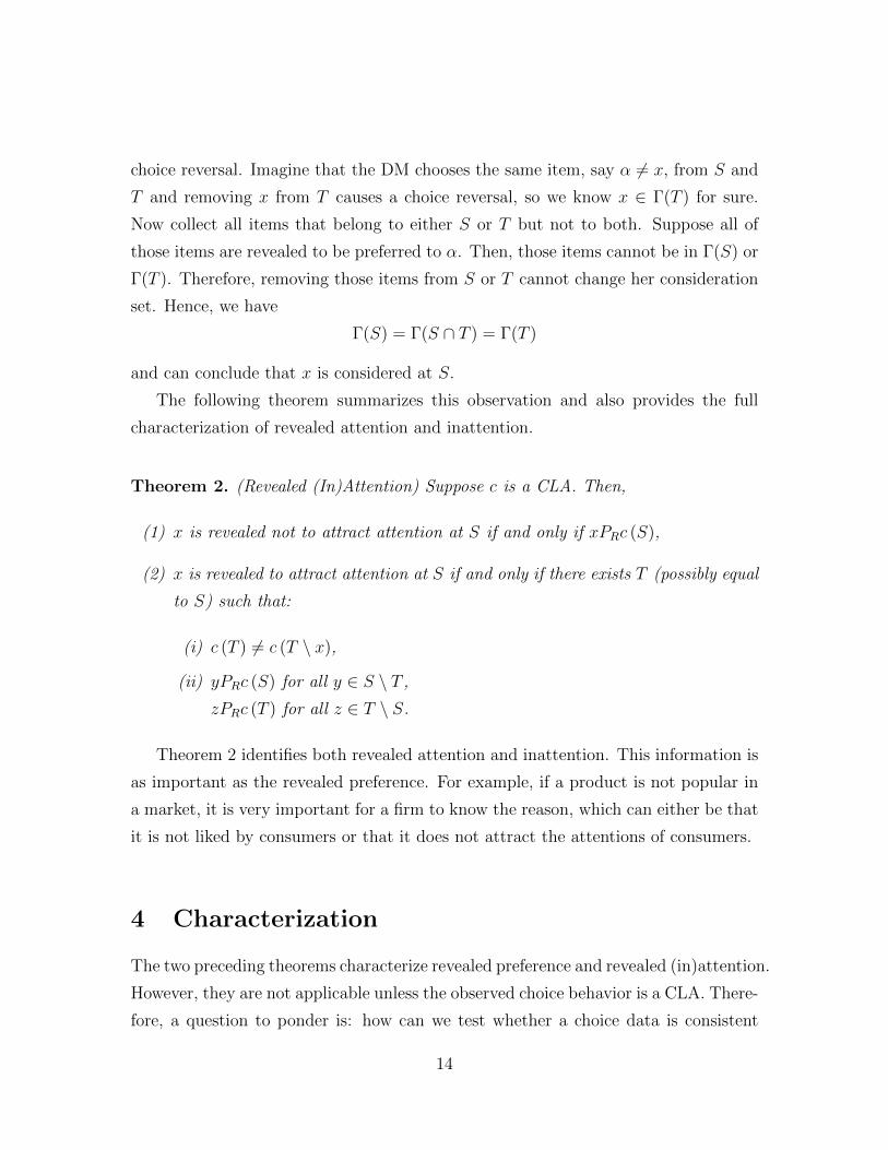
Theorem 2. (Revealed (In)Attention) Suppose c is a CLA. Then,

(1) x is revealed not to attract attention at S if and only if xPRc (S),

(2) x is revealed to attract attention at S if and only if there exists T (possibly equal

to S) such that:

(i) c (T ) 6= c (T \ x),

(ii) yPRc (S) for all y ∈ S \ T ,

zPRc (T ) for all z ∈ T \ S.

Theorem 2 identifies both revealed attention and inattention. This information is

as important as the revealed preference. For example, if a product is not popular in

a market, it is very important for a firm to know the reason, which can either be that

it is not liked by consumers or that it does not attract the attentions of consumers.

4 Characterization

The two preceding theorems characterize revealed preference and revealed (in)attention.

However, they are not applicable unless the observed choice behavior is a CLA. There-

fore, a question to ponder is: how can we test whether a choice data is consistent

14

with CLA? Surprisingly, it turns out that CLA can be simply characterized by only

one observable property of choice.

Before we state the property, recall the sufficient and necessary condition for

observed behavior to be consistent with the preference maximization under the full

attention assumption: the Weak Axiom of Revealed Preference (WARP). WARP is

equivalent to stating that every set S has the “best” alternative x∗ in the sense that

it must be chosen from any set T whenever x∗ is available and the choice from T lies

in S. Formally,

WARP: For any nonempty S, there exists x∗ ∈ S such that for any T

including x∗,

c(T ) = x∗ whenever c(T ) ∈ S.

Because of the full attention assumption, being feasible is equal to attracting

attention. However, this is no longer true when we allow for the possibility of limited

attention. To conclude that x∗ is chosen from T , we not only need to make sure

that the chosen element from T is in S and x∗ is available but also that x∗ attracts

attention. As we have discussed, we can infer this when removing x∗ from T changes

the DM’s choice, which is the additional requirement for x∗ to be chosen from T .

This discussion suggests the following axiom, which is a weakening of WARP:

WARP with Limited Attention - WARP(LA): For any nonempty

S, there exists x∗ ∈ S such that, for any T including x∗,

c(T ) = x∗ whenever (i) c(T ) ∈ S, and(ii) c(T ) 6= c(T \ x∗)

WARP with Limited Attention indeed guarantees that the binary relation P de-

fined in (1) is acyclic and it fully characterizes the class of choice functions generated

by an attention filter. The next lemma makes it clear that WARP(LA) is equivalent

to the fact that P has no cycle.

Lemma 1. P is acyclic if and only if c satisfies WARP with Limited Attention.

Proof. (The if-part) Suppose P has a cycle: x1Px2P · · ·PxkPx1. Then for each

i = 1, . . . , k − 1 there exists Ti such that xi = c(Ti) 6= c(Ti \ xi+1) and xk = c(Tk) 6=

15

c(Tk \ x1). Consider the set {x1, . . . , xk} ≡ S. Then, for every x ∈ S, there exists

T such that c(T ) ∈ S and c(T \ x) 6= c(T ) but x 6= c(T ), so WARP with Limited

Attention is violated.

(The only-if part) Suppose P is acyclic. Then every S has at least one element

x such that there is no y ∈ S with yPx, which means that there is no y ∈ S with

y = c(T ) 6= c(T \ x). Equivalently, whenever c(T ) ∈ S and c(T ) 6= c(T \ x), it must

be x = c(T ), which is WARP with Limited Attention.

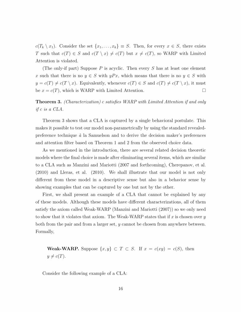
Theorem 3. (Characterization) c satisfies WARP with Limited Attention if and only

if c is a CLA.

Theorem 3 shows that a CLA is captured by a single behavioral postulate. This

makes it possible to test our model non-parametrically by using the standard revealed-

preference technique a la Samuelson and to derive the decision maker’s preferences

and attention filter based on Theorem 1 and 2 from the observed choice data.

As we mentioned in the introduction, there are several related decision theoretic

models where the final choice is made after eliminating several items, which are similar

to a CLA such as Manzini and Mariotti (2007 and forthcoming), Cherepanov, et al.

(2010) and Lleras, et al. (2010). We shall illustrate that our model is not only

different from these model in a descriptive sense but also in a behavior sense by

showing examples that can be captured by one but not by the other.

First, we shall present an example of a CLA that cannot be explained by any

of these models. Although these models have different characterizations, all of them

satisfy the axiom called Weak-WARP (Manzini and Mariotti (2007)) so we only need

to show that it violates that axiom. The Weak-WARP states that if x is chosen over y

both from the pair and from a larger set, y cannot be chosen from anywhere between.

Formally,

Weak-WARP. Suppose {x, y} ⊂ T ⊂ S. If x = c(xy) = c(S), then

y 6= c(T ).

Consider the following example of a CLA:

16

Example 2. There are four alternatives x, y, a, b. The alternatives a and b are never

chosen (unless there is no other alternative) but they alter the attention of the decision

maker. Her preference is y � x � a � b and picks the best alternative from those

she considers. She considers y only when either a or b is feasible but not both and

always considers all other alternatives. It is easy to see that her consideration set

mapping is an attention filter so her choice function satisfies WARP(LA). However,

it does not satisfy Weak-WARP because c(xy) = c(xyab) = x (y is not considered)

but c(xya) = y.

Conversely, none of the above alternative models is a special case of the CLA

model. In Example 3, we present a model of Rational Shortlist Method of Manzini

and Mariotti (2007) that cannot be a CLA. One can easily verify that the exactly same

choice function can be generated by other models mentioned above. The rational

shortlist model consists of two rationales P1 and P2 where P1 has no cycle (not

necessarily transitive) and P2 is a complete and transitive order.16 The decision is

made applying these rationales sequentially to eliminate alternatives. Consider the

following example of the rational shortlist model:

Example 3. The first rationale (not transitive17) and the second rationale (transitive)

are:

tP1y, yP1x, zP1x, zP1s

sP2xP2yP2zP2t

For instance, if the feasible set is {s, y, z}, s is eliminated in the first stage by z

and she picks y in the second stage by comparing y and z according to P2. However,

this choice function generates contradictory revealed preferences if it was a CLA:

• zP t since z = c(yzt) and y = c(yz),

16Actually, Manzini and Mariotti (2007) does not require the second rationale (P2) to be completeand transitive (it only requires P2 to be asymmetric). We put the stronger requirement on P2 inorder to highlight that the difference between these models is generated by the first stage, not by theincompleteness or intransitivity of the second rationale, which corresponds to the DM’s preferencein our model.

17One can show that if P1 is transitive, the first stage elimination generates an attention filter sothe resulting choice will be a CLA as long as P2 is complete and transitive.

17

• tPy since t = c(xyt) and x = c(xt),

• yPz since y = c(syz) and s = c(sy).

Thus, it cannot be explained by a CLA by Lemma 1. Hence, this choice cannot be

a part of our model.

5 Anomalies

Our limited attention model is capable of accommodating several frequently observed

behaviors: Attraction Effect, Cyclical Choice, and Choosing Pairwisely Unchosen.

Our explanations for these choice patterns solely depend on limited attention, hence

seemingly irrational behaviors can be explained without introducing changing prefer-

ence. We will overview them and illustrate how our model accommodates them. In

addition to that, we elicit the DM’s preference, attention and inattention from such

choice data.

Attraction Effect

The attraction effect refers to a phenomenon where adding an irrelevant alternative

to a choice set affects the choice.18 A typical attraction effect choice patterns is

c(xyd) = y, c(xy) = x, c(yd) = y, c(xd) = x.

Here d is the irrelevant alternative that shifts the choice from x to y. Thus, d is the

decoy of y. Donald R. Lehmann and Yigang Pan (1994) experimentally show that

introducing new products causes an attraction effect particularly by affecting the

composition of consideration sets. How the CLA model accommodates the attraction

effect is in line with their findings. One possible representation is that the DM’s

preference is y � x � d and she considers y only when d is present (otherwise, she

18This phenomenon is well-documented and robust in behavioral research on marketing (JoelHuber, John W. Payne and Christopher Puto (1982), Amos Tversky and Itamar Simonson (1993)),including in choice among monetary gambles, political candidates, job candidates, environmentalissues, and medical decision making. Advertising irrelevant alternatives is commonly used as amarketing strategy to invoke the attraction effect on the customers.

18

considers everything). It is clear that her consideration set mapping is an attention

filter.

Now we elicit the preference of a decision maker whose choice behavior follows

the same pattern above without knowing her preference and consideration sets. By

Theorem 1, y = c(xyd) 6= c(xy) imply that y is revealed to be preferred to d. That

is, our model judges that she prefers y over its own decoy.

One can naturally imagine the attraction effect with more than one decoy. How-

ever most of the theoretical literature cannot accommodate it,19 but our model can.

Consider there are two decoys dx and dy of x and y, respectively. That is,

c(xydxdy) = x, c(xydy) = y, c(xy) = x.

The CLA model can accommodate this behavior: she considers y only when dy is

present but dx is not. She ignores x when dy is available but not dx. Then she will

exhibit the above choice as long as she prefers x over dx and y over dy.

Again, assume we have no prior information about the DM’s preference and consid-

eration sets. The first two choices reveal that she pays attention to dx at {x, y, dx, dy}so prefers x over dx. Similarly, the second and third tell us she prefers y over dy.

Therefore, our approach again elicits her preference between an alternative and its

decoy.

Cyclical Choice

Kenneth O. May (1954) provides the first experiment where cyclical choice pat-

terns are observed and these results have been replicated in many different choice

environments (e.g. Tversky (1969), Graham Loomes, Chris Starmer, and Robert

Sugden (1969), Manzini and Mariotti (2009a), Michael Mandler, Manzini and Mari-

otti (2009)). Consider a cyclical choice pattern:

c(xyz) = x, c(xy) = x, c(yz) = y, c(xz) = z.

We have already illustrated that this choice patter can be captured by our model

19This generalized attraction effect is another example that lies outside of recent models providedin Cherepanov, et al. (2008), Manzini and Mariotti (forthcoming) and Lleras, et al. (2010) since itdoes not satisfy Weak-WARP. There are two exceptions: Efe A. Ok, Pietro Ortoleva and Gil Riella(2010) and Geoffroy de Clippel and Eliaz (2010). However, these two models can accommodateneither Cyclical nor Choosing Pairwisely choice patterns.

19

at the beginning of Section 3. Now let us elicit the preference. Since the DM exhibits

a choice reversal when y is removed from {x, y, z}, we can identify that y attracts her

attention when these three elements are present. So, we can conclude that she prefers

x over y. However, as illustrated before, we cannot determine the ranking of z.

Choosing Pairwisely Unchosen

In this choice pattern, the DM chooses an alternative that is never chosen from

pairwise comparisons:

c(xyz) = z, c(xy) = x, c(yz) = y, c(xz) = x.

Since removing x or y from {x, y, z} changes her choice, it is revealed that z is

better than x and y but we cannot determine her preference between x and y. Since

her revealed preference has no cycle, her behavior is captured by our model through

Lemma 1 and Theorem 3.

Note that the best element, z, is not chosen in any binary choice so we can conclude

that she pays attention to z only when x and y are present. Applying Theorem 2, we

can pin down her consideration set uniquely except when her feasible set is {x, y}:

Revealed Preference zPRx and zPRy

xyz xy yz xz

Revealed Attention xyz x y x

Revealed Inattention - - z z

Table 2: Choosing Pairwisely Unchosen

One possible story that generates such an attention pattern is “searching more

when the decision is tough.” Several items are hard to find even if they are feasible.

The decision maker first considers alternatives that are feasible and easy to find and

if there is an item that dominates all others, she chooses it immediately. Otherwise,

she makes an extensive search to find all feasible items. In the former case, the

consideration set consists only of easily found (and feasible) alternatives and in the

latter case it coincides with the feasible set. Given this story, suppose her true

preference is z � x � y where the decision between x and y is very tough and z is

hard to find. She makes an extensive search to find z only if she sees both x and y.

If either x or y is missing, she does not bother to search, and therefore overlooks z.

20

6 Further Comments

In this section, we discuss the boundaries of our method. First of all, our revealed

preference could be very incomplete, in other words, it only provides coarse welfare

judgements. In the extreme case where the choice data satisfies WARP, Theorem

1 and Theorem 2 do not provide any identification of the preference and atten-

tion/inattention. This is because the DM’s behavior can be attributed fully to her

preference or to her inattention (always considering her actual choice). Thus, we can-

not make any statement without imposing any additional assumption. This extreme

example illustrates the limitation of choice data, which alone is not enough to identify

her preferences. Notice that the classical revealed preference is not an exception since

it implicitly assumes the full attention.

Nevertheless, a policy maker may be forced to make a welfare judgement even

when our revealed preference is silent. There are three directions to deal with incom-

pleteness of our revealed preference: (1) looking for additional data other than choice

data, (2) imposing additional structures on attention filter, and/or (3) utilizing other

methods as long as the resulting revealed preference includes ours. We will discuss

each of them in detail.

� Additional Data: The idea of our (direct) revealed preference is that we can

conclude x is preferred to y if x is chosen while y gets an attention, which is inferred

when removing y changes her choice. However, if we know y is considered for some

other reason, we will naturally make the same conclusion even without observing

such a choice change. One can get such an information from many sources such as

eye-tracking, fMRI and the tracking system in the internet commerce.20 If the policy

maker believes that these sources are trustable, he can utilize them to get extra

revealed preferences. We now illustrate how it can be combined with our revealed

preference.

Assume a policy maker has an extra piece of information about consumer’s pref-

erence. For instance, the choice data may not reveal her ranking between x and y

but some laboratory experiment or survey study may have already found that she

20In this regard, our theory highlights the importance of other tools (besides the observed choices)which can shed light on the choice process rather than outcome.

21

prefers x over y. In such a case, the policy maker can add x � y to the revealed

preference generated by our method (Theorem 1), say P ′ = PR ∪ {(x, y)}. By using

the transitive closure of P ′, denoted by P ′R, the policy maker can obtain more atten-

tion/inattention information like Theorem 2. Indeed, Theorem 1 and 2 are exactly

applicable by replacing PR with the transitive closure of P ′R.

Similarly, a policy maker may know she pays attention to x under certain deci-

sion problem. This information immediately generates more information about her

preference, (the chosen element here is better than x), which tells more about her

attention/inattention like in the previous case.

� Further Restrictions on Consideration Sets: The other direction is to impose

additional restrictions on Γ other than being an attention filter. For example, if the

source of limited attention is simply the abundance of alternatives, one reasonable

restriction is that the decision maker considers at least two alternatives for each de-

cision problem as a benchmark. That is |Γ(S)| > 2. Under this restriction, the choice

data reveals her preference completely. This result is trivial but still it is important

for a marketer to find whether an unchosen alternative attracts attention. Our ap-

proach will provide an answer for the revealed attention. The revealed attention and

inattention will be characterized by Theorem 2 by replacing PR with the completely

identified preference.

Notice that the classical revealed preference can be seen as one of such an attempt

with the strongest assumption on the consideration set Γ(S) = S. Our model high-

lights that we need to assume how choices are made in order to make a meaningful

revealed preference exercise. The assumption about what are chosen (like WARP) is

not enough.

� Other Methods: One can combine our methodology with others which try to

make the welfare analysis without relying on a particular choice procedure, such as

Apesteguia and Ballester (2010) and Bernheim and Rangel (2009). What is common

between our model and theirs is that all try to respect consumer’s choice for the

welfare judgment as much as possible. The difference is that our model does so only

when the consumer actually considers other unchosen alternatives.

Now imagine that a policy maker knows/believes a consumer behaves according to

22

our model. Then, he should first elicit her preference based on our method. Admit-

tedly, it only provides an incomplete ranking (and empty if the choice data satisfies

WARP). If the policy maker is forced to make a complete welfare judgement with

a risk of making mistakes, he can apply the other methods with the constraint of

respecting the revealed preference generated by our model. In other words, these

methods should be used only to break the incompleteness of our revealed preference.

For instance, consider Apesteguia and Ballester’s approach. They first axiomati-

cally construct an index to measure the consistency between choice data and a certain

preference, and of all complete and transitive preferences pick the one that minimizes

the inconsistency for the welfare analysis. However, if the policy maker knows the

decision maker follows a choice with limited attention, he should first elicit her pref-

erence based on our method and then pick the inconsistency-minimizing preference

only from those that are consistent with our revealed preference. The resulting welfare

judgment can be wrong (can be different from her actual preference). Nevertheless,

this sequential process eliminates certain mistakes the policy maker would make if

he simply applied the other model-free methods. For instance, applying Apesteguia

and Ballester’s approach directly to Example 1 will lead the wrong conclusion: y is

welfare improving over x but this sequential advocacy certainly kills such a mistake.

7 Concluding Remarks

Limited attention has been widely studied in economics: neglecting the nontranspar-

ent taxes (Raj Chetty, Adam Looney, and Kory Kroft (2009)), inattention to released

information (Stefano DellaVigna and Joshua Pollet (2007)), costly information ac-

quisition (Xavier Gabaix, et al. (2006)), and rational inattention in macroeconomics

(Christopher A. Sims (2003)). For example, Goeree (2008) shows that relaxing the

full attention assumption by allowing customers to be unaware of some computers in

the market is enough to explain the high markups in the PC industry.

In this paper, we study the implications of limited attention on revealed preference.

We illustrate when and how one can deduce both the preference and consideration sets

of a DM who follows a CLA. The distinction between a preference and an (in)attention

is crucial. For instance, if a product is not popular in a market, it is very important

23

for a firm to know the reason, which can either be that it is not liked by consumers or

that it does not attract the attentions of consumers. Our model provides a theoretical

framework to distinguish these two possibilities. Similarly, a social planner can find

a proper strategy to make sure that people choose the right option in 401(K) plans

and health insurance. Hence, in a welfare analysis it is important to understand the

underlying model of the DM.

Since revealed preference and (in)attention are the main focus of the paper, we

impose a rather weak restriction on consideration sets. Such a weak condition allows

us to apply our revealed preference and (in)attention theorems to seemingly irrational

choice patterns (i.e. Attraction Effect, Cyclical Choice, and Choosing Pairwisely

Unchosen). Nevertheless, depending on the intended application, our framework can

be used to analyze choices under different restrictions on consideration sets.

� In many real-world markets, products compete with each other for the space

in the consideration set of the DM, who has cognitive limitations. In these situations,

if an alternative attracts attention when there exist many others, then it is easier to

be considered when some of other alternatives become unavailable. If a product is

able to attract attention in a crowded supermarket shelf, the same product will be

noticed when there are fewer alternatives, i.e., x ∈ Γ(T ) implies x ∈ Γ(S) whenever

x ∈ S ⊂ T . Lleras, et al. (2010) extensively study consideration sets which satisfy

this property. They also consider the cases where both conditions are satisfied.

� Lleras, et al. (2010) also consider another special case whereby the decision

maker overlooks or disregards an alternative because it is dominated by another item

in some aspect. Imagine Maryland’s economics department is hiring one tenure-

track theorist. Since there are too many candidates in the job market to consider

all of them, the department asks other departments to recommend their best theory

student. Therefore, a candidate from Michigan is ignored if and only if there is

another Michigan candidate who is rated better by Michigan. In this case, Maryland’s

filter is represented by a irreflexive and transitive order as long as each department’s

ranking over its students is rational. Formally, given an irreflexive and transitive

(possible incomplete) order �, the attention filter consists of alternatives which are

undominated with respect to this order, Γ�(S) = {x ∈ S| @y ∈ S s.t. y � x} .

24

8 References

Ambrus, Attila, and Kareen Rozen. 2010. “Revealed Conflicting Preferences:Rationalizing Choice with Multi-Self Models.” Unpublished.

Apesteguia, Jose, and Miguel A. Ballester. 2008. “A Characterization ofSequential Rationalizability.” Economics Working Papers, Universitat Autonoma deBarcelona 1089.

Apesteguia, Jose, and Miguel A. Ballester. 2010. “A Measure of Rationalityand Welfare.” Unpublished.

Aumann, Robert J. 2005. “Musings on Information and Knowledge.” EconJournal Watch, 2(1), 88-96.

Basar, Gozen and Chandra Bhat. 2004. “A Parameterized ConsiderationSet Model for Airport Choice: An Application to the San Francisco Bay Area.”Transportation Research Part B: Methodological, 38 (10), 889-904.

Bernheim, B. Douglas, and Antonio Rangel. 2007. “Toward Choice-Theoretic Foundations for Behavioral Welfare Economics.” American Economic Re-view, 2007, 97(2), 464-470.

Bernheim, B. Douglas, and Antonio Rangel. 2009. “Beyond Revealed Pref-erence: Choice-Theoretic Foundations for Behavioral Welfare Economics.” QuarterlyJournal of Economics, 124(1), 51-104.

Broadbent, Donald E. 1958. Perception and Communication. New York: Perg-amon Press.

Caplin, Andrew, and Mark Dean. Forthcoming. “Search, Choice, and Re-vealed Preference.” Theoretical Economics.

Caplin, Andrew, Mark Dean, and Daniel Martin. Forthcoming. “Searchand Satisficing.” American Economic Review.

Chambers, Christopher P., and Takashi Hayashi. 2008. “Choice and Indi-vidual Welfare.” HSS California Institute of Technology Working Paper 1286.

Cherepanov, Vadim, Timothy Feddersen, and Alvaro Sandroni. 2010.“Rationalization.” Unpublished.

Chetty, Raj, Adam Looney, and Kory Kroft. 2009. “Salience and Taxation:Theory and Evidence.” American Economic Review, 99(4), 1145-1177.

Chiang, Jeongwen, Siddhartha Chib, and Chakravarthi Narasimhan.1998. “Markov Chain Monte Carlo and Models of Consideration Set and ParameterHeterogeneity.” Journal of Econometrics, 89 (1-2), 223-248.

Dawes, Philip L. and Jennifer Brown. 2005. “The Composition of Consider-ation and Choice Sets in Undergraduate University Choice: An Exploratory Study,”Journal of Marketing for Higher Education, 14(2), 37-59.

de Clippel, Geoffroy, and Kfir Eliaz. 2010. “Reason-Based Choice: A Bar-gaining Rationale for the Attraction and Compromise Effects.” Unpublished.

DellaVigna, Stefano, and Joshua Pollet. 2007. “Demographics and Industry

25

Returns.” American Economic Review, 97, 1167-1702.Dulleck, Uwe, Franz Hackl, Bernhard Weiss, and Rudolf Winter-Ebmer.

2008. “Buying Online: Sequential Decision Making by Shopbot Visitors.” Institutfur Hohere Studien, Wien Economics Series 225.

Eliaz, Kfir, Michael Richter, and Ariel Rubinstein. Forthcoming. “AnEtude in Choice Theory: Choosing the Two Finalists.” Economic Theory.

Eliaz, Kfir and Ran Spiegler. Forthcoming. “Consideration Sets and Com-petitive Marketing.” Review of Economic Studies.

Filiz-Ozbay, Emel. 2008. “Incorporating Awareness into Contract Theory.”Unpublished.

Gabaix, Xavier, David Laibson, Guillermo Moloche, and Stephen Wein-berg. 2006. “Costly Information Acquisition: Experimental Analysis of a BoundedlyRational Model.” American Economic Review, 96 (4), 1043-1068.

Goeree, Michelle S. 2008. “Limited Information and Advertising in the USPersonal Computer Industry.” Econometrica, 76, 1017-1074.

Green, Jerry R., and Daniel Hojman. 2008. “Choice, Rationality and Wel-fare Measurement.” Harvard Institute of Economic Research Discussion Paper No.2144.

Hauser, John R., and Birger Wernerfelt. 1990. “An Evaluation Cost Modelof Evoked Sets.” Journal of Consumer Research, 16, 383-408.

Hausman, Daniel. 2008. “Mindless or Mindfull Economics: A MethodologicalEvaluation.” In The Foundations of Positive and Normative Economics: A Handbook,ed. Andrew Caplin and Andrew Schotter, 125-155, New York: Oxford UniversityPress.

Heifetz, Aviad, Martin Meier, and Burkhard C. Schipper. 2010. “Dy-namic Unawareness and Rationalizable Behavior.” Unpublished.

Hotchkiss, Gord, Steve Jensen, Manoj Jasra, and Doug Wilson. 2004.“The Role of Search in Business to Business Buying Decisions A Summary of ResearchConducted.” Unpublished.

Houy, Nicolas. 2007. “Rationality and Order-Dependent Sequential Rational-ity.” Theory and Decision, 62 (2), 119-134.

Houy, Nicolas, and Koichi Tadenuma. 2009. “Lexicographic Compositionsof Multiple Criteria for Decision Making.” Journal of Economic Theory, 144 (4),1770-1782.

Huber, Joel, John W. Payne, and Christopher Puto. 1982. “AddingAsymmetrically Dominated Alternatives: Violations of Regularity and the SimilarityHypothesis.” Journal of Consumer Research, 9 (1), 90-98.

Huberman, Gur, and Tomer Regev. 2001. “Contagious Speculation and aCure for Cancer: A Nonevent that Made Stock Prices Soar.” Journal of Finance, 56(1), 387-396.

Lavidge, Robert J., and Gary A. Steiner. 1961. “A model for Predictive

26

Measurements of Advertising Effectiveness,” Journal of Marketing, 25, 59-62.Lehmann, Donald R., and Yigang Pan. 1994. “Context Effects, New Brand

Entry, and Consideration Sets.” Journal of Marketing Research, 31 (3), 364-374.Lleras, Juan S., Yusufcan Masatlioglu, Daisuke Nakajima, and Erkut Y.

Ozbay. 2010. “When More is Less: Choice by Limited Consideration.” Unpublished.Loomes, Graham, Chris Starmer, and Robert Sugden. 1991. “Observing

Violations of Transitivity by Experimental Methods.” Econometrica, 59 (2), 425-439.Mandler, Michael, Paola Manzini, and Marco Mariotti. 2010. “A Million

Answers to Twenty Questions: Choosing by Checklist.” Unpublished.Manzini, Paola, and Marco Mariotti. 2007. “Sequentially Rationalizable

Choice.” American Economic Review, 97 (5), 1824-1839.Manzini, Paola, and Marco Mariotti. 2009a. “Choice over Time.” In Oxford

Handbook of Rational and Social Choice, ed. Paul Anand, Prastanta Pattanaik, andClemens Puppe, Chapter 10, New York: Oxford University Press.

Manzini, Paola, and Marco Mariotti. 2009b. “Choice based welfare eco-nomics for boundedly rational agents,” Unpublished.

Manzini, Paola, and Marco Mariotti. Forthcoming. “Categorize ThenChoose: Boundedly Rational Choice and Welfare.” Journal of the European Eco-nomic Association.

Masatlioglu, Yusufcan, and Daisuke Nakajima. 2009. “Choice by IterativeSearch.” Unpublished.

May, Kenneth O. 1954. “Intransitivity, Utility, and the Aggregation of Prefer-ence Patterns.” Econometrica, 22, 1-13.

Noor, Jawwad. Forthcoming. “Temptation and Revealed Preference.” Econo-metrica.

Ok, Efe A., Pietro Ortoleva, and Gil Riella, 2010. “Revealed (P)ReferenceTheory.” Unpublished.

Ozbay, Erkut Y. 2008. “Unawareness and Strategic Announcements in Gameswith Uncertainty.” Unpublished.

Pessemier, Edgar A. 1978. “Stochastic Properties of Changing Preferences.”American Economic Review, 68 (2), 380-385.

Richards, Max D., John E. Sheridan, and John W. Slocum. 1975 “Com-parative Analysis of Expectancy and Heuristic Models of Decision Behavior.” Journalof Applied Psychology, 60 (3), 361-368.

Roberts, John H., and James M. Lattin. 1991. “Development and Testingof a Model of Consideration Set Composition.” Journal of Marketing Research, 28(4), 429-440.

Rubinstein, Ariel, and Yuval Salant. 2010. “Eliciting Welfare Preferencesfrom Behavioral Datasets.” Unpublished.

Salant, Yuval and Ariel Rubinstein. 2008. “Choice with Frames.” Review ofEconomic Studies, 75, 1287-1296.

27

Samuelson, Paul A. 1938. “A Note on the Pure Theory of Consumers’ Behav-ior.” Econometrica, 61-71.

Simon, Herbert A., 1957. Models of Man: Social and Rational: MathematicalEssays on Rational Human Behavior in a Social Setting. New York: John Wiley andSons, Inc.

Sims, Christopher A. 2003. “Implications of Rational Inattention.” Journal ofMonetary Economics, 50 (3), 665-690.

Stigler, George J. 1961. “The Economics of Information.” Journal of PoliticalEconomy, 69 (3), 213-225.

Tversky, Amos. 1969. “Intransitivity of Preferences.” Psychological Review,76, 31-48.

Tversky, Amos, and Itamar Simonson. 1993. “Context-Dependent Prefer-ences.” Management Science, 39 (10), 1179-1189.

Varian, Hal R.. 2006. “Revealed Preference.” In Samuelsonian Economicsand the Twenty-First Century, ed. Michael Szenberg, Lall Ramrattan, and Aron A.Gottesman, 99-115, New York: Oxford University Press.

Wright, Peter, and Fredrick Barbour. 1977. “Phased Decision Strategies:Sequels to an Initial Screening.” In Studies in Management Sciences, Multiple Cri-teria Decision Making, ed. Martin K. Starr, and Milan Zeleny, 91-109, Amsterdam:North-Holland.

Zyman, Sergio. 1999. The End of Marketing as We Know It. New York: HarperCollins.

28

9 Appendix

The Proofs of Theorem 1, Theorem 2 and Theorem 3

Notice that the if-parts of Theorem 1 and Theorem 2 have been already shown in themain text. The following proofs use these results.

Proof of Theorem 3

Suppose c is a CLA represented by (�,Γ). Then Theorem 1(if part) implies that� must include P so P must be acyclic. Therefore, by Lemma 1, c must satisfyWARP(LA).

Now suppose that c satisfies WARP(LA). By Lemma 1, P is acyclic so there is apreference � that includes P . Pick any such preference arbitrarily and define

Γ(S) = {x ∈ S : c(S) � x} ∪ {c(S)} (2)

Then, it is clear that c(S) is the unique �-best element in Γ(S) so all we need toshow is that Γ is an attention filter. Suppose x ∈ S but x 6∈ Γ(S) (so x 6= c(S)). Byconstruction, x � c(S) so it cannot be c(S)Px. Hence, it must be c(S) = c(S \ x) sowe have Γ(S) = Γ(S \ x). �

Proof of Theorem 1 (The Only-If part)

Suppose xPRy does not hold. Then there exists a preference that includes PR andranks y better than x. The proof of Theorem 3 shows that c can be represented bysuch a preference so x is not revealed to be preferred to y. �

Proof of Theorem 2 (The Only-If parts)

(Revealed Inattention) Suppose x is not revealed to be preferred to c(S). Then picka preference that includes PR and puts c(S) above x. The proof of Theorem 3 showsthat c can be represented by such a preference and an attention filter Γ with x ∈ Γ(S).

(Revealed Attention) Suppose there exists no T which satisfies the condition. Weshall prove that if c is a CLA then it can be represented by some attention filterΓ with x 6∈ Γ(S). If c(S)PRx does not hold, we have already shown that c can berepresented with x � c(S) and x 6∈ Γ(S) so x is not revealed to attract attention atS, so we focus on the case when c(S)PRx.

Now construct a binary relation, P , where aP b if and only if “aPRb” or “a = c(S)and not bPRc(S).” That is, P puts c(S) as high as possible as long as it does notcontradict PR. Since PR is acyclic and c is represented by an attention filter, one canshow that P is also acyclic. Given this, take any preference relation � that includes

29

P , which includes PR as well. We have already shown that Γ(S) ≡ {z ∈ S : c(S) �z} ∪ {c(S)} is an attention filter and (Γ,�) represents c. Now define Γ as follows :

Γ (S ′) =

{Γ (S ′) for S ′ /∈ D

Γ (S ′) \ x for S ′ ∈ Dwhere D is a collections of sets such that

D =

{S ′ ⊂ X :

c (S ′) = c (S) andzPRc (S ) for all z ∈ (S \ S ′) ∪ (S ′ \ S)

}That is, Γ is obtained from Γ by removing from x any budget set S ′ where c(S) =

c(S ′) and any item that belongs to S or S ′ but not to both is revealed to be better thanc(S). Notice that x cannot be c(S) because if this true, the condition of the statementis satisfied for T = S. Hence, Γ(S ′) ⊂ Γ(S ′) always includes c(S ′). Furthermore theproof of Theorem 3 shows that (Γ,�) represents c. Therefore, (Γ,�) also representsc so we only need to show that Γ is an attention filter.

To do that, it is useful to notice that Γ is an attention filter and c(T ′) = c(T ′′)whenever Γ(T ′) = Γ(T ′′) because (Γ,�) represents c.

Suppose y 6∈ Γ(T ). We shall prove Γ(T ) = Γ(T \ y).

Case I: y = xIf T 6∈ D, then we have Γ(T ) = Γ(T ) = Γ(T \ x) = Γ(T \ x). If T ∈ D, then it

must be c(T ) = c(T \ x) (otherwise, the condition of the statement is satisfied) so byconstruction of Γ and Γ, we have Γ(T ) = Γ(T ) \ x = Γ(T \ x) = Γ(T \ x).

Case II: T ∈ D and y 6= xSince y 6∈ Γ(T ) is equivalent to y 6∈ Γ(T ), we have Γ(T ) = Γ(T \ y). Therefore,

c(T \ y) = c(T ) = c(S). By construction of Γ and Γ, it must be y � c(S), whichimplies yPRc(S) by construction of �. Therefore, T \ y ∈ D. Therefore, Γ(T ) =Γ(T ) \ x = Γ(T \ y) \ x = Γ(T \ y).

Case III: T 6∈ D and y 6= xIf T \ y ∈ D, analogously to the previous case, we have c(T ) = c(T \ y) = c(S)

and yPRc(S) so it must be T ∈ D, which is a contradiction. Hence, T \ y 6∈ D so wehave Γ(T ) = Γ(T ) = Γ(T \ y) = Γ(T \ y). �

30