Embed Size (px)
Citation preview

International Association
Of Certified
Practicing Engineers
www.iacpe.com
Setting The Standard
Page : 1 of 76
Rev: 01
Rev. 01 – Dec 2015
IACPE
No 19, Jalan Bilal Mahmood 80100 Johor Bahru Malaysia
PHYSICS AND ELECTROMAGNETISM
CPE LEVEL I
TRAINING MODULE
The International Association of Certified Practicing Engineers is providing the introduction to the Training Module for your review. We believe you should consider joining our Association and becoming a Certified Practicing Engineer. This would be a great option for engineering improvement, certification and networking. This would help your career by
1. Providing a standard of professional competence in the practicing engineering and management field
2. Identify and recognize those individuals who, by studying and passing an examination, meets the standards of the organization
3. Encourage practicing engineers and management professionals to participate in a continuing program of personal and professional development
www.IACPE.com
International Association
Of Certified
Practicing Engineers
PHYSICS AND ELECTROMAGNETISM
CPE LEVEL I
TRAINING MODULE
Page 2 of 76
Rev: 01
December 2015
TABLE OF CONTENT
INTRODUCTION 8
Scope 8
General Considerations 9
A. Magnet and Magnetism 9
B. Magnetic Field 12
C. Magnetic Materials and Magnetic Properties 17
DEFINITIONS 23
NOMENCLATURE 25
Greek Letter 25
THEORY 26
A. Electromagnetism 26 1. Magnetic Flux 28 2. Magnetic Flux Density 28 3. Magnetomotive Force and Magnetic Flux Intensity 31 4. Permeability 32 5. Reluctance 33 6. B-H Curve and Hysteresis Loop 35 7. Polarity 39 8. Electromagnetism Induction 41
B. Maxwell Equations 49
C. Magnetostatics 53
1. Current and Current Density 53 2. Ohm’s Law 54 3. Resistance 55 4. Power and Joule’s Law 56 5. Postulates of Magnetostatic 58
International Association
Of Certified
Practicing Engineers
PHYSICS AND ELECTROMAGNETISM
CPE LEVEL I
TRAINING MODULE
Page 3 of 76
Rev: 01
December 2015
D. Electromagnet Radiation 60 1. Wave Properties 64 2. Doppler Effect 67 3. Planck’s Curve 68
E. Electromagnet Application 70
1. Electric Bell 71 2. Relay 72 3. Lifting Magnet 73 4. Telephone Receiver 74
REFERENCE 75
LIST OF TABLE
Table 1: Properties of Permanent Magnets 21
Table 2: Relative Permeability μ of Selected Materials at Zero Frequency
and at Room Temperature 32
Table 3: Electrical Conductivity σ and Temperature Coefficient α
(Near 20oC) for selected material at DC 55
International Association
Of Certified
Practicing Engineers
PHYSICS AND ELECTROMAGNETISM
CPE LEVEL I
TRAINING MODULE
Page 4 of 76
Rev: 01
December 2015
LIST OF FIGURE
Figure 1: Electron spinning around nucleus produces magnetic field 9
Figure 2: Electrostatic and Magnetostatic force 10
Figure 3: Magnetic Domains 11
Figure 4: The law of Magnetic Attraction and Repulsion 12
Figure 5: Bar Magnet 12
Figure 6: Magnetic Field 13
Figure 7: Magnetic Field of a bar magnet 14
Figure 8: Magnetic Field Lines on Bar Magnet 15
Figure 9: Magornetic Field Lines for Fields Involving Two Magnet 16
Figure 10: Magnetic Field Lines in a Uniform Field 17
Figure 11: Magnetic Field Produced by Current, I 26
Figure 12: Magnetic Field Produced by Coil 27
Figure 13: Hysteresis Loop 29
Figure 14: The Magnetic Circuit 30
Figure 15: Different Physical Forms of Electromagnets 34
Figure 16: Typical B-H Curve for Two Types of Soft Iron 35
Figure 17: Hysteresis Loss 37
Figure 18: Magnetic Field Produced by Current in a Conductor 39
Figure 19: The Left-hand rule for current Carrying conductors 39
International Association
Of Certified
Practicing Engineers
PHYSICS AND ELECTROMAGNETISM
CPE LEVEL I
TRAINING MODULE
Page 5 of 76
Rev: 01
December 2015
Figure 20: Left-hand rule for Coils 40
Figure 21: Left-hand rule to find North Pole of an Electromagnet 41
Figure 22: Induced EMF 42
Figure 23: Electromagnet Induction 43
Figure 24: Magnetic Field Rotating Around Wire 44
Figure 25: Wire in the Coil 44
Figure 26: A Short Selenoid 46
Figure 27: A Toroid Inductor 46
Figure 28: A Closely Wound Toroidal Coil 47
Figure 29: A Circuit illustrating Self-Inductance 48
Figure 30: Self-Propagating Electromagnetic Curve 50
Figure 31: The Left-Hand Rule 51
Figure 32: Conductor 55
Figure 33: Electro magnetic radiation 61
Figure 34: Visible Spectrum 62
Figure 35: Visual and radio Window of Electromagnetic Radiation 63
Figure 36: Reflection and Refraction 64
Figure 37: Raindrop 65
Figure 38: Phenomenon of Diffraction 66
Figure 39: Doppler Effect 67
Figure 40: Types of Spectrum Emitted 68
Figure 41: Plack’s Curve 70
International Association
Of Certified
Practicing Engineers
PHYSICS AND ELECTROMAGNETISM
CPE LEVEL I
TRAINING MODULE
Page 6 of 76
Rev: 01
December 2015
Figure 42: Electric Bell 71
Figure 43: Relay 72
Figure 44: Lifting Magnet 73
Figure 45: Telephone Receiver 74
International Association
Of Certified
Practicing Engineers
PHYSICS AND ELECTROMAGNETISM
CPE LEVEL I
TRAINING MODULE
Page 7 of 76
Rev: 01
December 2015
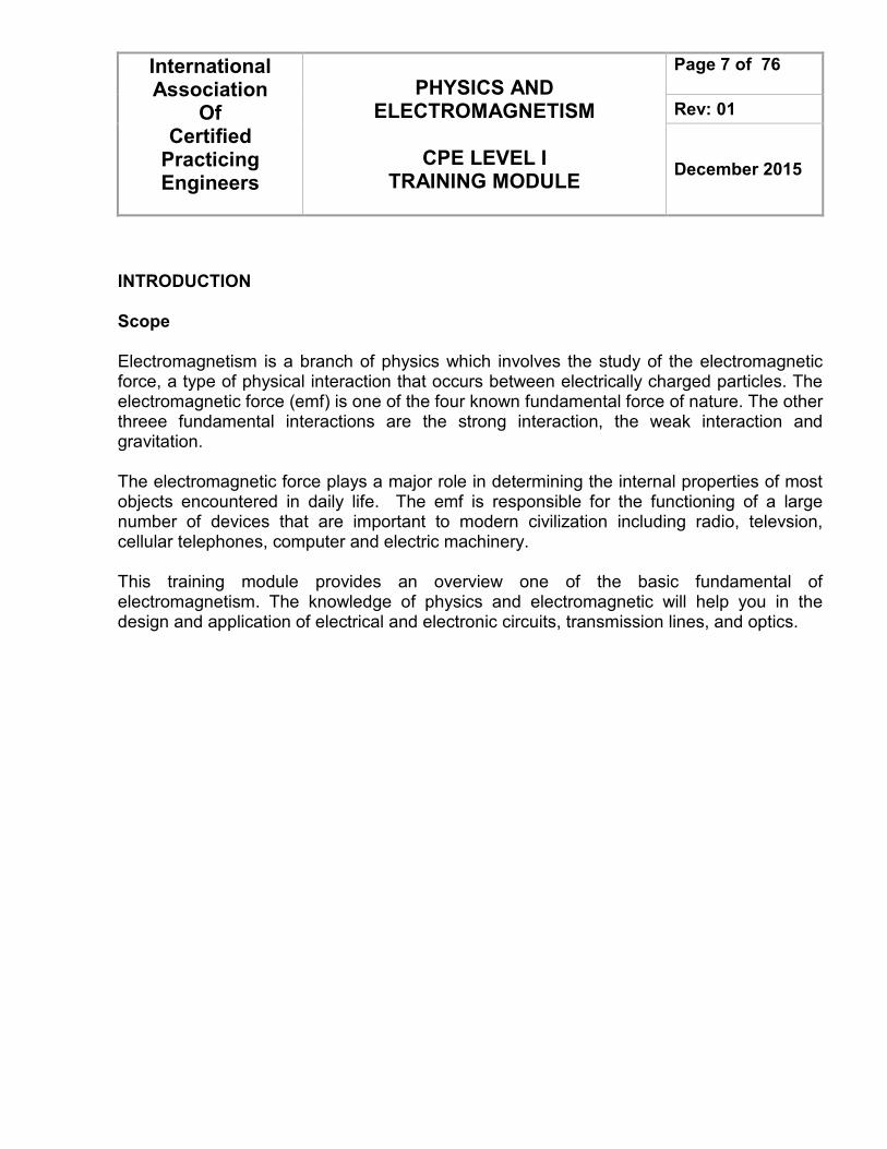
INTRODUCTION Scope Electromagnetism is a branch of physics which involves the study of the electromagnetic force, a type of physical interaction that occurs between electrically charged particles. The electromagnetic force (emf) is one of the four known fundamental force of nature. The other threee fundamental interactions are the strong interaction, the weak interaction and gravitation. The electromagnetic force plays a major role in determining the internal properties of most objects encountered in daily life. The emf is responsible for the functioning of a large number of devices that are important to modern civilization including radio, televsion, cellular telephones, computer and electric machinery. This training module provides an overview one of the basic fundamental of electromagnetism. The knowledge of physics and electromagnetic will help you in the design and application of electrical and electronic circuits, transmission lines, and optics.
International Association
Of Certified
Practicing Engineers
PHYSICS AND ELECTROMAGNETISM
CPE LEVEL I
TRAINING MODULE
Page 8 of 76
Rev: 01
December 2015
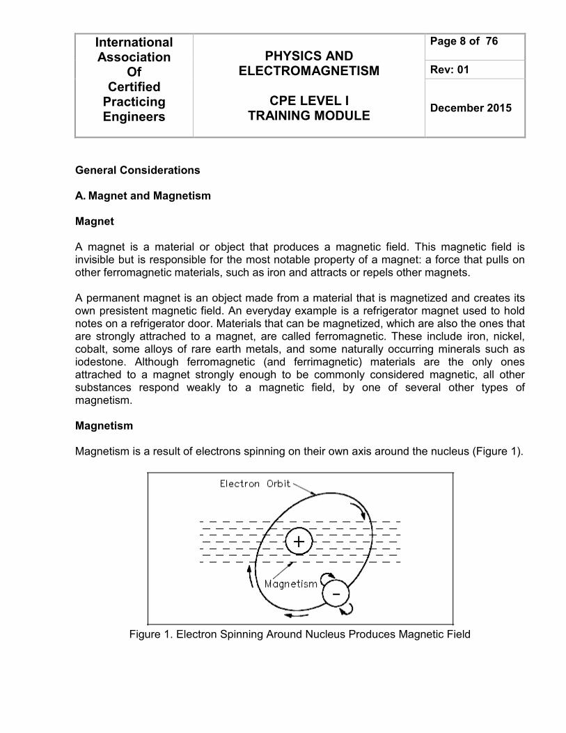
General Considerations A. Magnet and Magnetism Magnet A magnet is a material or object that produces a magnetic field. This magnetic field is invisible but is responsible for the most notable property of a magnet: a force that pulls on other ferromagnetic materials, such as iron and attracts or repels other magnets. A permanent magnet is an object made from a material that is magnetized and creates its own presistent magnetic field. An everyday example is a refrigerator magnet used to hold notes on a refrigerator door. Materials that can be magnetized, which are also the ones that are strongly attrached to a magnet, are called ferromagnetic. These include iron, nickel, cobalt, some alloys of rare earth metals, and some naturally occurring minerals such as iodestone. Although ferromagnetic (and ferrimagnetic) materials are the only ones attrached to a magnet strongly enough to be commonly considered magnetic, all other substances respond weakly to a magnetic field, by one of several other types of magnetism. Magnetism Magnetism is a result of electrons spinning on their own axis around the nucleus (Figure 1).
Figure 1. Electron Spinning Around Nucleus Produces Magnetic Field
International Association
Of Certified
Practicing Engineers
PHYSICS AND ELECTROMAGNETISM
CPE LEVEL I
TRAINING MODULE
Page 9 of 76
Rev: 01
December 2015
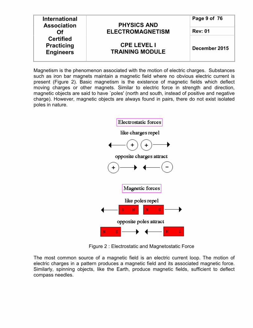
Magnetism is the phenomenon associated with the motion of electric charges. Substances such as iron bar magnets maintain a magnetic field where no obvious electric current is present (Figure 2). Basic magnetism is the existence of magnetic fields which deflect moving charges or other magnets. Similar to electric force in strength and direction, magnetic objects are said to have `poles' (north and south, instead of positive and negative charge). However, magnetic objects are always found in pairs, there do not exist isolated poles in nature.
Figure 2 : Electrostatic and Magnetostatic Force
The most common source of a magnetic field is an electric current loop. The motion of electric charges in a pattern produces a magnetic field and its associated magnetic force. Similarly, spinning objects, like the Earth, produce magnetic fields, sufficient to deflect compass needles.
International Association
Of Certified
Practicing Engineers
PHYSICS AND ELECTROMAGNETISM
CPE LEVEL I
TRAINING MODULE
Page 10 of 76
Rev: 01
December 2015
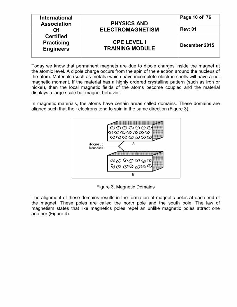
Today we know that permanent magnets are due to dipole charges inside the magnet at the atomic level. A dipole charge occurs from the spin of the electron around the nucleus of the atom. Materials (such as metals) which have incomplete electron shells will have a net magnetic moment. If the material has a highly ordered crystalline pattern (such as iron or nickel), then the local magnetic fields of the atoms become coupled and the material displays a large scale bar magnet behavior.
In magnetic materials, the atoms have certain areas called domains. These domains are aligned such that their electrons tend to spin in the same direction (Figure 3).
Figure 3. Magnetic Domains
The alignment of these domains results in the formation of magnetic poles at each end of the magnet. These poles are called the north pole and the south pole. The law of magnetism states that like magnetics poles repel an unlike magnetic poles attract one another (Figure 4).
International Association
Of Certified
Practicing Engineers
PHYSICS AND ELECTROMAGNETISM
CPE LEVEL I
TRAINING MODULE
Page 11 of 76
Rev: 01
December 2015
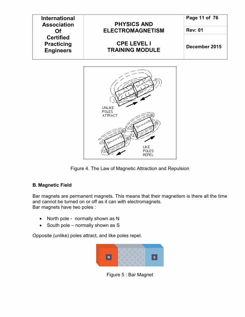
Figure 4. The Law of Magnetic Attraction and Repulsion
B. Magnetic Field Bar magnets are permanent magnets. This means that their magnetism is there all the time and cannot be turned on or off as it can with electromagnets. Bar magnets have two poles :
• North pole - normally shown as N
• South pole – normally shown as S
Opposite (unlike) poles attract, and like poles repel.
Figure 5 : Bar Magnet
International Association
Of Certified
Practicing Engineers
PHYSICS AND ELECTROMAGNETISM
CPE LEVEL I
TRAINING MODULE
Page 12 of 76
Rev: 01
December 2015
If permanent magnets are repeatedly knocked, the strength of their magnetic field is reduced. Converting a magnet to a non-magnet is called demagnetisation. Magnets are made from magnetic metals - iron, nickel and cobalt. These are the only pure metals that can be turned into a permanentmagnet. Steel is an alloy of iron and so can also be made into a magnet. If these metals have not been turned into a permanent magnet they will still be attracted to a magnet if placed within a magnetic field. In this situation they act as a magnet but only whilst in the magnetic field. This is called induced magnetism.
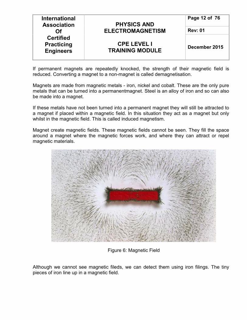
Magnet create magnetic fields. These magnetic fields cannot be seen. They fill the space around a magnet where the magnetic forces work, and where they can attract or repel magnetic materials.
Figure 6: Magnetic Field
Although we cannot see magnetic fileds, we can detect them using iron filings. The tiny pieces of iron line up in a magnetic field.
International Association
Of Certified
Practicing Engineers
PHYSICS AND ELECTROMAGNETISM
CPE LEVEL I
TRAINING MODULE
Page 13 of 76
Rev: 01
December 2015
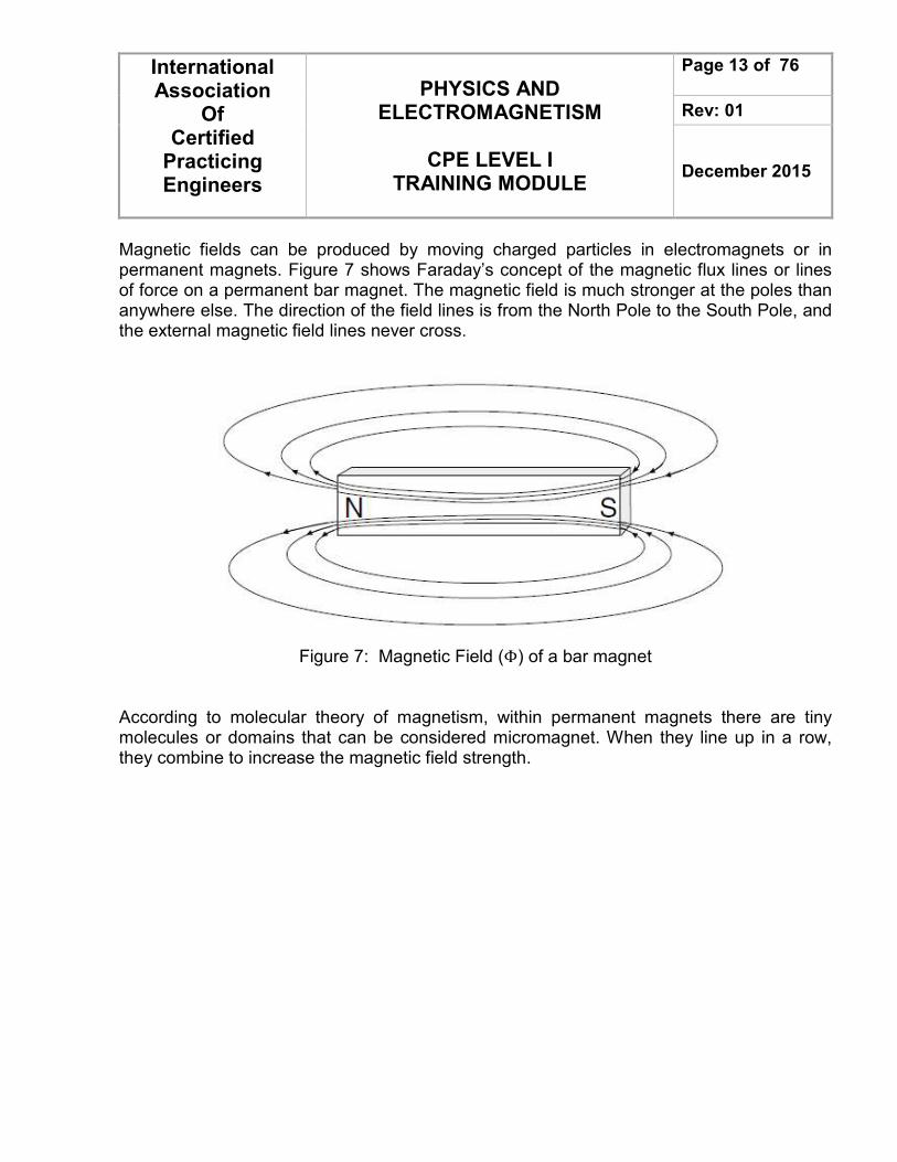
Magnetic fields can be produced by moving charged particles in electromagnets or in permanent magnets. Figure 7 shows Faraday’s concept of the magnetic flux lines or lines of force on a permanent bar magnet. The magnetic field is much stronger at the poles than anywhere else. The direction of the field lines is from the North Pole to the South Pole, and the external magnetic field lines never cross.
Figure 7: Magnetic Field (Φ) of a bar magnet
According to molecular theory of magnetism, within permanent magnets there are tiny molecules or domains that can be considered micromagnet. When they line up in a row, they combine to increase the magnetic field strength.
International Association
Of Certified
Practicing Engineers
PHYSICS AND ELECTROMAGNETISM
CPE LEVEL I
TRAINING MODULE
Page 14 of 76
Rev: 01
December 2015
Drawing Magnetic Field Diagram
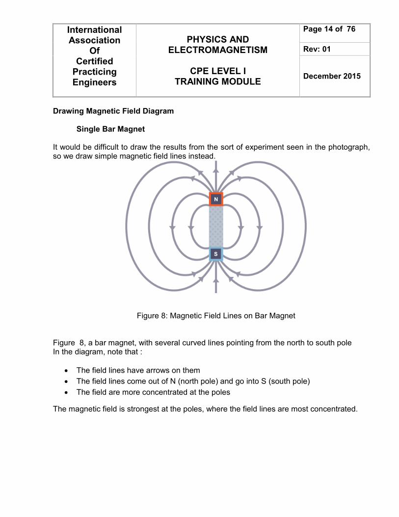
Single Bar Magnet It would be difficult to draw the results from the sort of experiment seen in the photograph, so we draw simple magnetic field lines instead.
Figure 8: Magnetic Field Lines on Bar Magnet
Figure 8, a bar magnet, with several curved lines pointing from the north to south pole In the diagram, note that :
• The field lines have arrows on them
• The field lines come out of N (north pole) and go into S (south pole)
• The field are more concentrated at the poles
The magnetic field is strongest at the poles, where the field lines are most concentrated.
International Association
Of Certified
Practicing Engineers
PHYSICS AND ELECTROMAGNETISM
CPE LEVEL I
TRAINING MODULE
Page 15 of 76
Rev: 01
December 2015
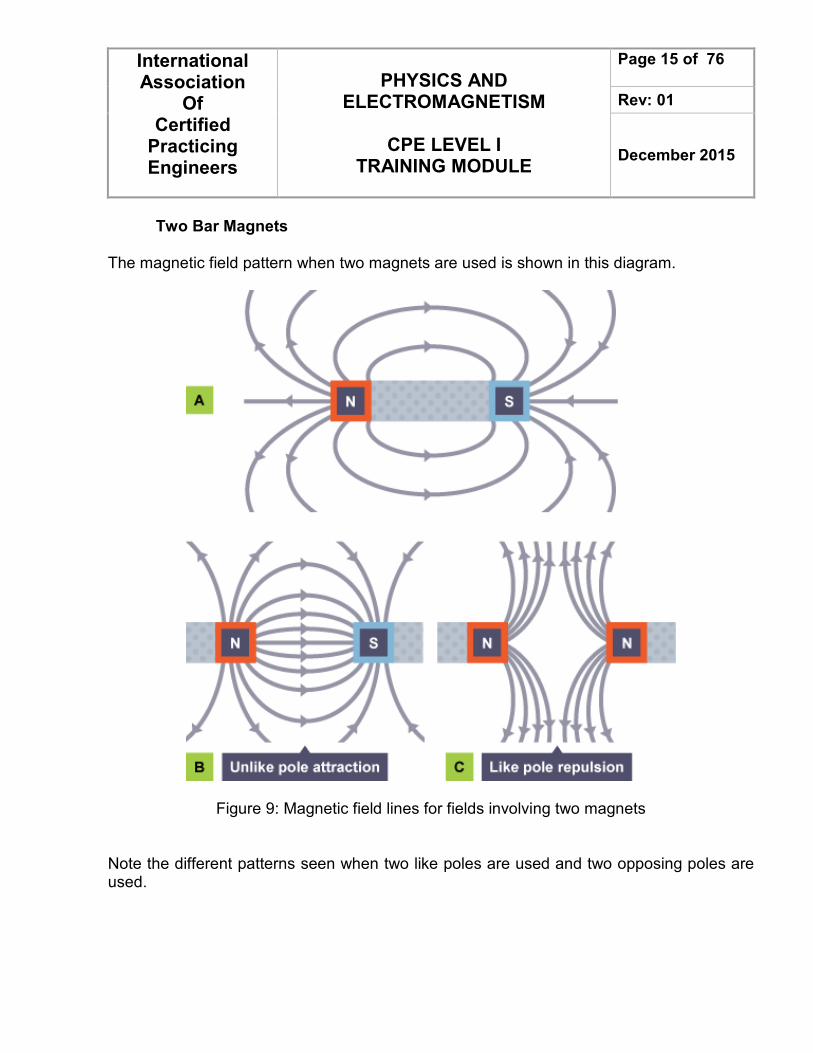
Two Bar Magnets
The magnetic field pattern when two magnets are used is shown in this diagram.
Figure 9: Magnetic field lines for fields involving two magnets
Note the different patterns seen when two like poles are used and two opposing poles are used.
International Association
Of Certified
Practicing Engineers
PHYSICS AND ELECTROMAGNETISM
CPE LEVEL I
TRAINING MODULE
Page 16 of 76
Rev: 01
December 2015
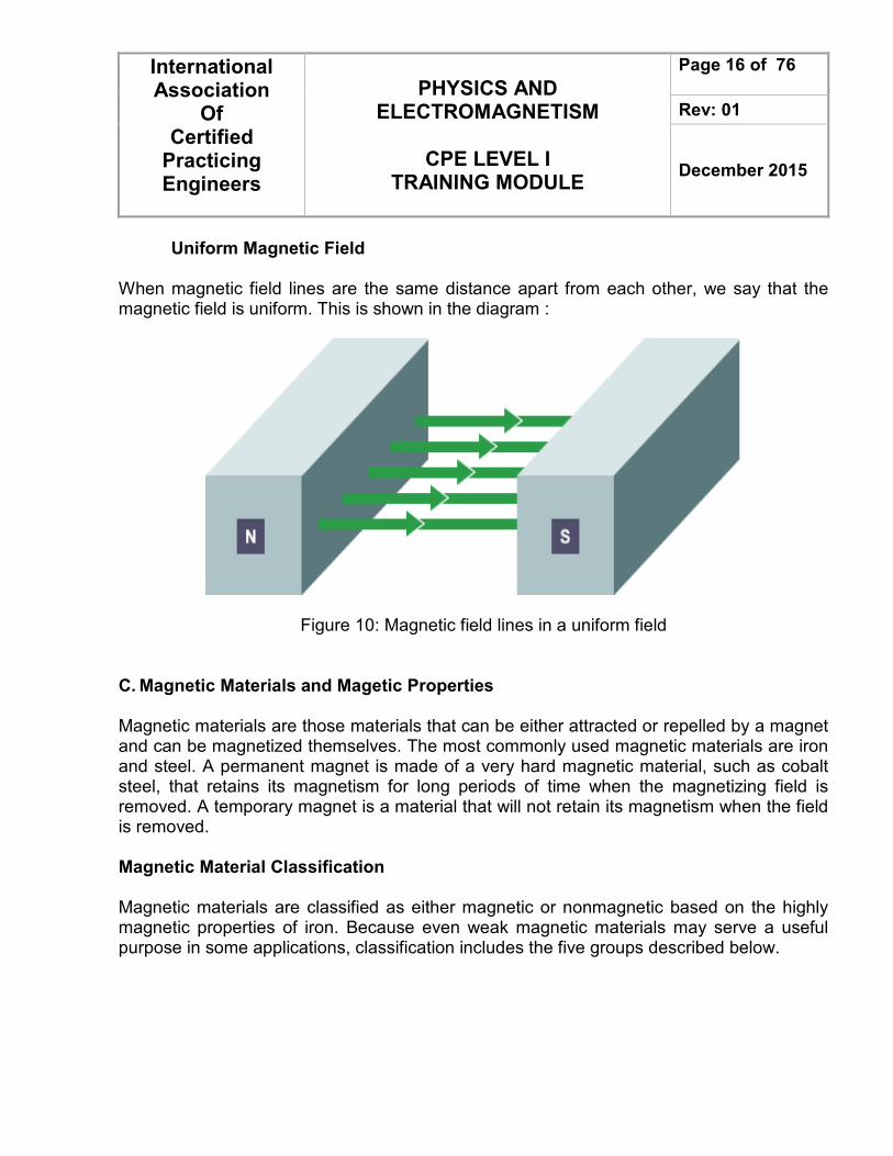
Uniform Magnetic Field
When magnetic field lines are the same distance apart from each other, we say that the magnetic field is uniform. This is shown in the diagram :
Figure 10: Magnetic field lines in a uniform field C. Magnetic Materials and Magetic Properties
Magnetic materials are those materials that can be either attracted or repelled by a magnet and can be magnetized themselves. The most commonly used magnetic materials are iron and steel. A permanent magnet is made of a very hard magnetic material, such as cobalt steel, that retains its magnetism for long periods of time when the magnetizing field is removed. A temporary magnet is a material that will not retain its magnetism when the field is removed. Magnetic Material Classification Magnetic materials are classified as either magnetic or nonmagnetic based on the highly magnetic properties of iron. Because even weak magnetic materials may serve a useful purpose in some applications, classification includes the five groups described below.
International Association
Of Certified
Practicing Engineers
PHYSICS AND ELECTROMAGNETISM
CPE LEVEL I
TRAINING MODULE
Page 17 of 76
Rev: 01
December 2015
• Diamagnetic Materials
All materials are diamagnetic to some extent although this behaviour may be
superceded by a more dominant effect, such as ferromagnetism. Diamagnetism is a
classical effect produced by moving charges. The induced magnetization M is
opposed to the applied B, thus reducing the total B in such a material sample. This
effect is directly analogous to the polarization effects in ordinary dielectrics. These
are materials such as bismuth, antimony, copper, zinc, mercury, gold, and silver.
These materials have a relative permeability of less than one.
• Paramagnetic Materials
Paramagnetism is a quantum mechanical effect largely due to the spin magnetic moment of the electron. These are materials such as alumunium, platinum, maganese, and chromium. These materials have a relative permeability of slihtly more than one.
• Ferromagnetic Materials
There is a much stronger quantum mechanical interaction between neighboring spin
moments than with paramagnetic materials. Some of the feromagnetic or
nonmagnetic materials used are iron, steel, nickel, cobalt and the commercial alloys,
alnico and peralloy. Ferrites are nonmagnetic, but have the ferromagnetic properties
of iron. Ferrities are made of ceramic material and have relative permeabilities that
range from 50 to 200. They are commonly used in the coils for RF (Ratio Frequency)
transformers.
International Association
Of Certified
Practicing Engineers
PHYSICS AND ELECTROMAGNETISM
CPE LEVEL I
TRAINING MODULE
Page 18 of 76
Rev: 01
December 2015
Magnetic Properties
• Low Carbon Steels
Low carbon steel provides the path for the magnetic flux in most electrical machines :
generators, transformers and motors. Low carbon steel is used because of its high
permeability, this is, a large amount of flux can be produced with the expenditure of minimal
magnetizing “effort”, and it has low hystersis thus minimizing losses associated with the
magnetic field. High levels of flux mean more powerful machines can be produced for a
given size and weight.
• Hot – rolled steel
Electrical sheet steels from which the laminations are cut are produced by a process of
rolling in the steel mill. The steels have a crystalline structure and the magnetic properties
of the sheet are derived from the magnetic properties of the individual crystals or grains.
The grains themselves are anisotropic. That is, their properties differ according to the
direction along the crystall that these are measured.
• Grain – oriented steel
As early as the 1920s it had been recognized that if the individual steel crystals could be
aligned, a steel could be produced which, in one direction, would exhibit properties related
to the optimum magnetic properties of the crystals. This material is known as cold-rolled
grain-oriented steel. It is reduced in the steel mill by a hot rolling process until it is about 2
mm thick. Thereafter it is further reduced by a series of cold reductions interspersed with
annealing at around 900oC to around 0.3 mm final thickness. In order to reduce surface
oxidation and prevent the material sticking to the rolls, the steel is given a phosphate
coating in the mill. Gain-oriented steel has magnetic properties in the rolling direction which
are very much superior to those perpendicular to the rolling direction.
International Association
Of Certified
Practicing Engineers
PHYSICS AND ELECTROMAGNETISM
CPE LEVEL I
TRAINING MODULE
Page 19 of 76
Rev: 01
December 2015
• High – Permeability Steel
Cold-rolled steel as described above continued to be steadily improved until the end of
1960s when a further step-change was introduced by the Nippon Steel Corporation of
Japan. By introducing significant changes into the cold rolling process they achieved a
considerable improvement in the degree of grain orientation compared with the previous
grain-oriented material. This coating imparts a tensile stress into the steel which has the
effect of reducing hystersis loss. The reduces hystersis loss allows some reduction in the
amount of silicon which improves the workability of the material, reducing cutting burrs and
avoiding the need for these to be ground off. This coupled with the better insulation
properties of the coating means that additional; insulation is not required. The core
manufacturing process is simplified and the core itself has a better stacking factor.
• Domain-refined steel
Crystals of grain-oriented steel become aligned during the grain-orientation process in large
groups. These are known as domains. There is a protion of the core loss which is related to
the size of the domains so that this can be reduced by reducing the domain size. Domain
size can be reduced after cold rolling by introducing a small amount of stress into the
material. This is generally carried out by a process of laser etching so that this type of steel
is frequently referred to as laser-etched. Improvements to the rolling process have also
enabled this material to be produced in thinner sheets, down to 0.23 mm, with resulting
further reduction in eddy-current loss.
• Amorphous Steel
Amorphous steels have developed in a totally different direction to the silicon steels
described above. Amorphous steels have a non-crystalline structure. The atoms are
randomly distributed within the material. They are produced by very rapid cooling of the
molten alloy which contains about 20% of a glass forming element such as boron. The
material is generally produced by spraying a stream of molten alloy onto a rapidly rotating
copper drum. The molten material is cooled at the rate of about 106 degrees C per second
and solidifies to form a continuous thin ribbon. This requires annealing between 200 and
International Association
Of Certified
Practicing Engineers
PHYSICS AND ELECTROMAGNETISM
CPE LEVEL I
TRAINING MODULE
Page 20 of 76
Rev: 01
December 2015
280C to develop the required magnetic properties. The earlies quantities of the material
were only 2 mm wide and about 0.025 – 0.05 mm thick.
• Designation of core steels
Specification of magnetic materials including core steels is covered internationally by
standards. There is a multi-part document covering all aspect and types of magentic
materials used in the electrical industry.
• Permanet Magnets (Cast) Great advances have been made in the development of materials suitable for the production of permanent magnets. The earliest materials were tungsten and chromium steel, followed by the series of cobalt steels. Alni was the first of the alumunium-nickel-iron alloys to be discovered and with the addition of cobalt, titanium and niobium, the Alnico series of magnets was developed, the properties of which varied according to composition. These are hard and brittle and can only be shaped by grinding, although a certain amount of drilling is possible on certain composition after special heat treatment. The Permanent Magnet Association (disbanded March 1975) discovered that certain alloys when heat-treated in a strong magnetic field became anistropic. That is they develop high properties high properties in the direction of the field at the expense of properties in other direction.
• Permanent Magnets (Sintered) The techniques of powder metallurgy have been applied to both the isotropic and anisotropic Alnico types and it is possible to produce sintered permanet magnets which have approximatelly 10% poorer remanence and energy than cast magnets. More precise shapes are possible when using this method of production and it is economical for the production of large quantites of small magnets. Sintering techniques are also used to manufacture the oxide permanent magnets based on barium or strontium hexaferrite. These magnets which may be isotropic or anisotropic, have higher coercive force but lower remanence than the alloy magnets. They have the physical properties of ceramics, and inferior temperature stability, but their low cost makes them
International Association
Of Certified
Practicing Engineers
PHYSICS AND ELECTROMAGNETISM
CPE LEVEL I
TRAINING MODULE
Page 21 of 76
Rev: 01
December 2015
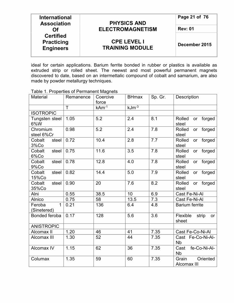
ideal for certain applications. Barium ferrite bonded in rubber or plastics is available as extruded strip or rolled sheet. The neewst and most powerful permanent magnets discovered to date, based on an intermettalic compound of cobalt and samarium, are also made by powder metallurgy techniques. Table 1. Properties of Permanent Magnets
Material Remanence Coercive force
BHmax Sp. Gr. Description
T kAm-1 kJm-3
ISOTROPIC
Tungsten steel 6%W
1.05 5.2 2.4 8.1 Rolled or forged steel
Chromium steel 6%Cr
0.98 5.2 2.4 7.8 Rolled or forged steel
Cobalt steel 3%Co
0.72 10.4 2.8 7.7 Rolled or forged steel
Cobalt steel 6%Co
0.75 11.6 3.5 7.8 Rolled or forged steel
Cobalt steel 9%Co
0.78 12.8 4.0 7.8 Rolled or forged steel
Cobalt steel 15%Co
0.82 14.4 5.0 7.9 Rolled or forged steel
Cobalt steel 35%Co
0.90 20 7.6 8.2 Rolled or forged steel
Alni 0.55 38.5 10 6.9 Cast Fe-Ni-Al
Alnico 0.75 58 13.5 7.3 Cast Fe-Ni-Al
Feroba 1 (Sinetered)
0.21 136 6.4 4.8 Barium ferrite
Bonded feroba 0.17 128 5.6 3.6 Flexible strip or sheet
ANISTROPIC
Alcomax II 1.20 46 41 7.35 Cast Fe-Co-Ni-Al
Alcomax III 1.30 52 44 7.35 Cast Fe-Co-Ni-Al-Nb
Alcomax IV 1.15 62 36 7.35 Cast fe-Co-Ni-Al-Nb
Columax 1.35 59 60 7.35 Grain Oriented Alcomax III
International Association
Of Certified
Practicing Engineers
PHYSICS AND ELECTROMAGNETISM
CPE LEVEL I
TRAINING MODULE
Page 22 of 76
Rev: 01
December 2015
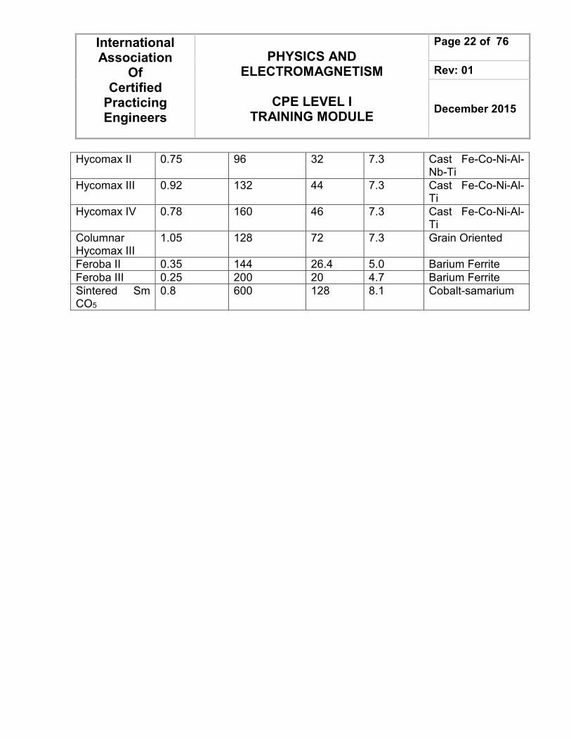
Hycomax II 0.75 96 32 7.3 Cast Fe-Co-Ni-Al-Nb-Ti
Hycomax III 0.92 132 44 7.3 Cast Fe-Co-Ni-Al-Ti
Hycomax IV 0.78 160 46 7.3 Cast Fe-Co-Ni-Al-Ti
Columnar Hycomax III
1.05 128 72 7.3 Grain Oriented
Feroba II 0.35 144 26.4 5.0 Barium Ferrite
Feroba III 0.25 200 20 4.7 Barium Ferrite
Sintered Sm CO5
0.8 600 128 8.1 Cobalt-samarium
International Association
Of Certified
Practicing Engineers
PHYSICS AND ELECTROMAGNETISM
CPE LEVEL I
TRAINING MODULE
Page 23 of 76
Rev: 01
December 2015
DEFINITIONS
Conductors – Materials with electrons that are loosely bound to their atoms, or materials that permit free motion of a large number of electron. Cosmic rays – Hghly penetrating particle rays from outer space. Current – The density of the atoms in copper wire is such that the valence orbits of the individual atoms overlap. Electromagnetic spectrum – EM radiant energy arranged in order of frequency or wavelength and divided into regions within which the waves have some common specified charachteristics. Gamma rays – Electromagnetic radiation of very high energy (greather than 30 keV) emitted after nuclear reactions or by a radioactive atom when it nucleus is left in an excited state after emission of alpha or beta particles. Inductance – The property which opposes any change in the existing current. Inductance is present only when the current is changing. Inductor – A conductor used to introduce inductance into a circuit. Insulators or nonconductors – Material with electrons that are tightly bound to their atoms and require large amounts of energy to free them from the influence of the nucleus. Light – white light, when split into a spectrum of colors, is composed of a continuous range of merging colors : red, orange, yellow, green, cyan, blue, indigo, and violet. Magnet – a vector that characterizes the magnet’s overall magnetic properties. Magnetic Flux – the group of magnetic field lines emitted outward from the north pole of magnet. Magnetic Flux Density – The amount of magnetic flux per unit area of a section, perpendicular to the direction to the direction of flux.
International Association
Of Certified
Practicing Engineers
PHYSICS AND ELECTROMAGNETISM
CPE LEVEL I
TRAINING MODULE
Page 24 of 76
Rev: 01
December 2015
Permanent magnet – an object made from a material that is magnetized and creates its own presistent magnetic field. Radio waves – Electromagnetic radiation suitable for radio transmission in the range of frequencies from about 10 kHz to about 300 MHz. Reflection – The abrupt change in the direction of propagation of a wave that strikes the boundary between different mediums. Refraction – The change in direction of a wave passing from one medium to another caused by its change in speed. Resistance – The ratio of the potential difference along a conductor to the current through the conductor Ultraviolet (UV) radiation – Electromagnetis radiations having wavelengths in the range from 0.4 nm to 3 nm. X Rays – Electromagnetic radiation of short wavelengths produced when cathode rays impinge on matter
International Association
Of Certified
Practicing Engineers
PHYSICS AND ELECTROMAGNETISM
CPE LEVEL I
TRAINING MODULE
Page 25 of 76
Rev: 01
December 2015
NOMENCLATURE A : Area of the cross section, m2
B : Magnetic flux density, tesla E : Electric field f : Frequency, Hz Fm : Magnetomotive force, mmf H : Field Intensity, At/m I : Current, Ampere J : Volume Current Density L : Length between poles of coil, m M : Mutual Inductance, H N : Number of turns q : Charge, C R : Reluctance, At/Wb t : Time, seconds v : Average velocity, m/s V : Voltage, V Greek Letter α :Temperature Coefficient μ : Permeability ε : Permetivity θ : Angle Φ : Magnetic flux, Webers σ : Electrical conductivity
International Association
Of Certified
Practicing Engineers
PHYSICS AND ELECTROMAGNETISM
CPE LEVEL I
TRAINING MODULE
Page 26 of 76
Rev: 01
December 2015
THEORY A. Electromagnetism Electromagnetism is a magnetic effect due to electric currents. When a compass is placed in close proximity to a wire carrying an electrical current, the comass needle will turn until it is at a right angle to the conductor the compass needle lines up in the direction of a magnetic field around the wire. It has been found that wires carrying current have the same type of magnetic field that exists around a magnet as shown in Figure 11.
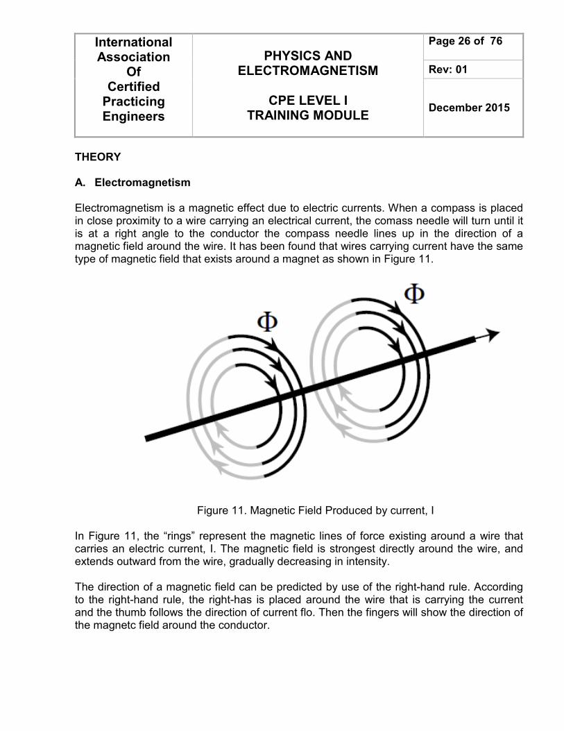
Figure 11. Magnetic Field Produced by current, I
In Figure 11, the “rings” represent the magnetic lines of force existing around a wire that carries an electric current, I. The magnetic field is strongest directly around the wire, and extends outward from the wire, gradually decreasing in intensity. The direction of a magnetic field can be predicted by use of the right-hand rule. According to the right-hand rule, the right-has is placed around the wire that is carrying the current and the thumb follows the direction of current flo. Then the fingers will show the direction of the magnetc field around the conductor.
International Association
Of Certified
Practicing Engineers
PHYSICS AND ELECTROMAGNETISM
CPE LEVEL I
TRAINING MODULE
Page 27 of 76
Rev: 01
December 2015
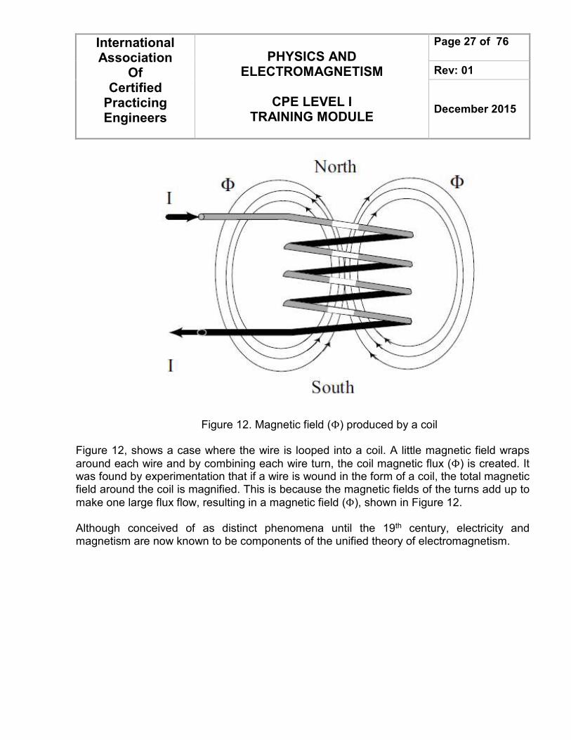
Figure 12. Magnetic field (Φ) produced by a coil
Figure 12, shows a case where the wire is looped into a coil. A little magnetic field wraps
around each wire and by combining each wire turn, the coil magnetic flux (Φ) is created. It was found by experimentation that if a wire is wound in the form of a coil, the total magnetic field around the coil is magnified. This is because the magnetic fields of the turns add up to
make one large flux flow, resulting in a magnetic field (Φ), shown in Figure 12. Although conceived of as distinct phenomena until the 19th century, electricity and magnetism are now known to be components of the unified theory of electromagnetism.
International Association
Of Certified
Practicing Engineers
PHYSICS AND ELECTROMAGNETISM
CPE LEVEL I
TRAINING MODULE
Page 28 of 76
Rev: 01
December 2015
1. Magnetic Flux
The group of magnetic field lines emitted outward from the north pole of a magnet is called
magnetic flux. The symbol of magnetic flux is Φ (phi). The SI unit of magnetic flux is the weber (Wb). One weber is equal to 1 x 10⁸ magnetic field lines.
2. Magnetic Flux Density
Magnetic flux density is the amount of magnetic flux per unit area of a section, perpendicular to the direction of flux. Equation (1) is the mathematical representation of magnetic flux density.
AB
φ=
(1) Where B = Magnetic flux density in teslas (T)
Φ = Magnetic flux in webers (Wb) A = Area in square meters (m2) The result is thet the SI unit for flux density is webers per square meter (Wb/m2). One weber per square meter equals one tesla. The field intensity and the resulting flux density are related through the permeability. The flux density is B = μ H (T) (2) Where μ is core permeability. The core permeability is a material constant describing the level of the flux in a material. When the material constant (μ) is high, the flux density will increase. The permeability has units of webers per ampere-turn-meter in the SI system.
The permeability of vacuum in free space is μo = 4π x 10-7 (Wb/At-m). When magnetic flux propagates through magnetic media, other than vacuum, the flux density is : B = μr μo H (T) (3)
International Association
Of Certified
Practicing Engineers
PHYSICS AND ELECTROMAGNETISM
CPE LEVEL I
TRAINING MODULE
Page 29 of 76
Rev: 01
December 2015
Where μr is the relative permeability. The relative permeability is 1 for a vacuum and can reach10,000 for ferromagnetic materials. Ferromagnetic materials have regions called domains of microscopic size.
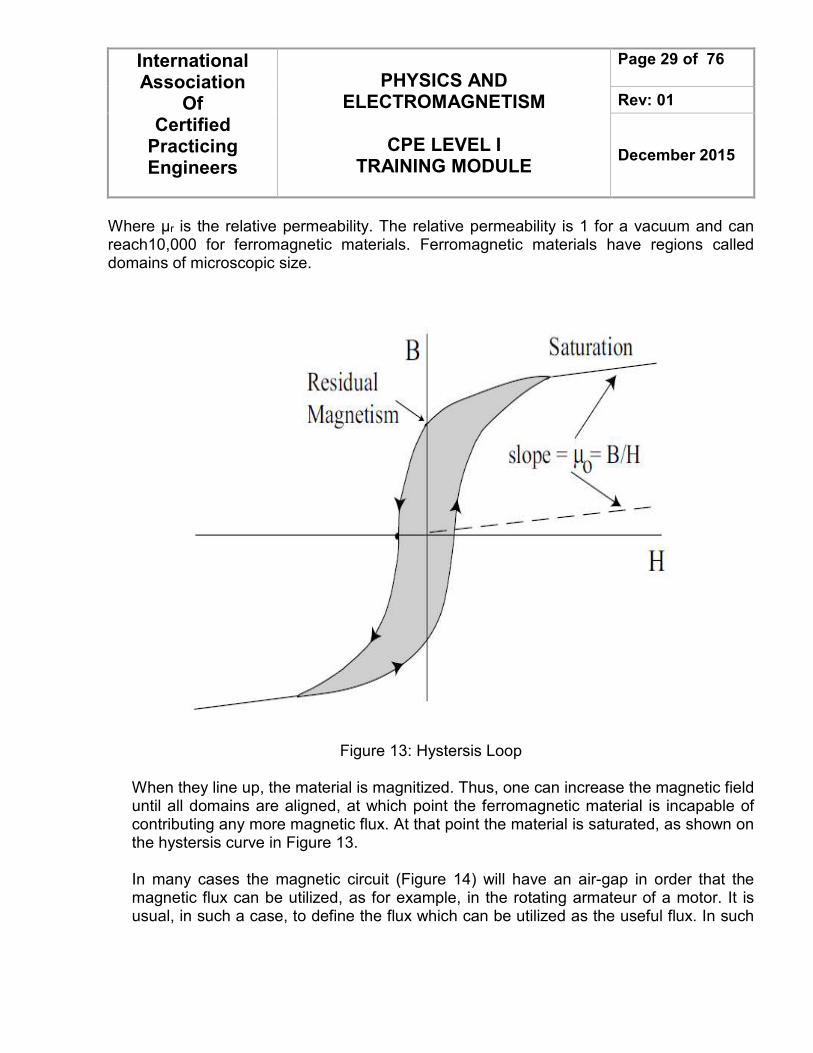
Figure 13: Hystersis Loop
When they line up, the material is magnitized. Thus, one can increase the magnetic field until all domains are aligned, at which point the ferromagnetic material is incapable of contributing any more magnetic flux. At that point the material is saturated, as shown on the hystersis curve in Figure 13. In many cases the magnetic circuit (Figure 14) will have an air-gap in order that the magnetic flux can be utilized, as for example, in the rotating armateur of a motor. It is usual, in such a case, to define the flux which can be utilized as the useful flux. In such
International Association
Of Certified
Practicing Engineers
PHYSICS AND ELECTROMAGNETISM
CPE LEVEL I
TRAINING MODULE
Page 30 of 76
Rev: 01
December 2015
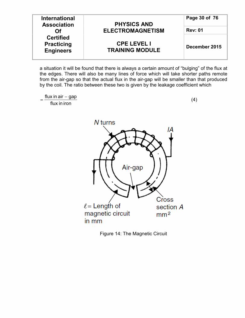
a situation it will be found that there is always a certain amount of “bulging” of the flux at the edges. There will also be many lines of force which will take shorter paths remote from the air-gap so that the actual flux in the air-gap will be smaller than that produced by the coil. The ratio between these two is given by the leakage coefficient which
iron in flux
gapair in flux −= (4)
Figure 14: The Magnetic Circuit
International Association
Of Certified
Practicing Engineers
PHYSICS AND ELECTROMAGNETISM
CPE LEVEL I
TRAINING MODULE
Page 31 of 76
Rev: 01
December 2015
3. Magnetomotive Force and Magnetic Field Intensity Magnetomotive Force
Magnetomotive force (mmf) is the strength of a magnetic field in a coil of wire. This is dependent on how much current flows in the turn coil: the more current, the stronger the magnetic field; the more turns of wire, the more concentrated the lines of force. The current times the number of turns of the coil is expressed in units called “ampere-turns” (At), also known as mmf. Equation (5) is the mathematical representation for ampere-turns (at). Fm = ampere – turns = NI (5) Where Fm = magnetomotive force (mmf) N = Number of turns I = Current, Ampere
Magnetic Field Intensity When a coil with a certain number of ampere-turn is stretched to twice its length, the magnetic file intensity, or the concentration of its magnetic lines of force, will be half as great. Therefore, field intensity depends on the length of the coil. Equation (6) is the mathematical representation for field intensity or magnetizing force, which is the mmf per unit length. The magnetic field inensity is written as:
L
NI
L
FH m == (6)
Where : H = Field Intensity (At/m) NI = Ampere-turns (At) L = Length between poles of coil (m) Fm = Magnetomotive force (mmf) Equation (6) describes an ability of a coil to produce magnetic flux.
International Association
Of Certified
Practicing Engineers
PHYSICS AND ELECTROMAGNETISM
CPE LEVEL I
TRAINING MODULE
Page 32 of 76
Rev: 01
December 2015
4. Permeability
Permeability (μ) is refers to the ability of a material to concentrate magnetic lines of flux. Those materials that can be easily magnetized are considered to have a high permeability. Relative permeability is the ratio of permeability of a material to the permeability of a vacuum (μo). The symbol for relative permeability is (μr).
o
or µ
µ=µ (7)
where μo = 2x10⁻⁷ H/m
Table 2: Relative Permeability μ of Selected Materials at Zero Fequency and at
Room Temperature
Material μr
Diamagnetic Water Copper Silver Gold Bismuth
0.99999 0.99999 0.99998 0.99996 0.99983
Paramagnetic Air Magnesium Alumunium Titanium FeO2
1.000004 1.000012 1.000021 1.00018 1.0014
Ferromagnetic Cobalt Nickel Mild Steel Iron Mumetal Supermalloy
250 600 2000 5000
100000 1000000
International Association
Of Certified
Practicing Engineers
PHYSICS AND ELECTROMAGNETISM
CPE LEVEL I
TRAINING MODULE
Page 33 of 76
Rev: 01
December 2015
5. Reluctance
Opposition to the production of flux in a material is called reluctance, which corresponds to resistance. The symbol for reluctance is R, and it has the units of ampere-turns per weber
(At/Wb). Reluctance is related to magnetomotive force, mmf and flux Φ by the relationship shown in equation (8)
φ=
mmfR
(8)
Reluctance is inversely proportional to permeability (μ). Iron coreshave high permeability and therefore, low reluctance. Air has a low permeability and, therefore a high reluctance. Equation (9) is the mathematical representation for reluctance
A
LR
µ= (9)
Where R = Reluctance, At/Wb L = Length of coil, m
μ = Permeability of magnetic material, ( )
At
mT −
A = Cross-sectional area of coil, m2
International Association
Of Certified
Practicing Engineers
PHYSICS AND ELECTROMAGNETISM
CPE LEVEL I
TRAINING MODULE
Page 34 of 76
Rev: 01
December 2015
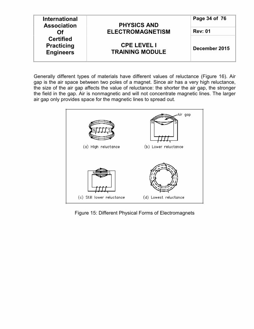
Generally different types of materials have different values of reluctance (Figure 16). Air gap is the air space between two poles of a magnet. Since air has a very high reluctance, the size of the air gap affects the value of reluctance: the shorter the air gap, the stronger the field in the gap. Air is nonmagnetic and will not concentrate magnetic lines. The larger air gap only provides space for the magnetic lines to spread out.
Figure 15: Different Physical Forms of Electromagnets

International Association
Of Certified
Practicing Engineers
PHYSICS AND ELECTROMAGNETISM
CPE LEVEL I
TRAINING MODULE
Page 35 of 76
Rev: 01
December 2015
6. B-H Curve and Hystersis Loop
The BH Magnetization Curve (Figure 16) shows how much flux density (B) results from increasing the flux intensity (H). The curves in Figure 16 are for two types of soft iron cores plotted for typical values. The curve for soft iron 1 shows that flux density B increases rapidly with an increase in flux intensity H, before the core saturates, or develops a “knee”. Thereafter, an increase in flux intensity H has little or no effect on flux density B. Soft iron 2 needs a much larger increase in flux intensity H before it reaches its saturation level at H = 5000 At/m, B = 0,3 T. Air, which is nonmagnetic, has a very low BH profile, as shown in Figure 16.
Figure 16. Typical BH Curve for Two Types of Soft Iron
International Association
Of Certified
Practicing Engineers
PHYSICS AND ELECTROMAGNETISM
CPE LEVEL I
TRAINING MODULE
Page 36 of 76
Rev: 01
December 2015
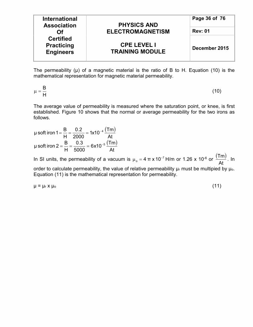
The permeability (μ) of a magnetic material is the ratio of B to H. Equation (10) is the mathematical representation for magnetic material permeability.
H
B=µ (10)
The average value of permeability is measured where the saturation point, or knee, is first established. Figure 10 shows that the normal or average permeability for the two irons as follows.
( )At
Tm10x1
2000
2.0
H
B1 iron soft μ 4−===
( )At
Tm10x6
5000
3.0
H
B2 iron soft μ 5−===
In SI units, the permeability of a vacuum is 7
o 10 x π 4 −=µ H/m or 1.26 x 10⁻⁶ or ( )At
Tm. In
order to calculate permeability, the value of relative permeability μr must be multipied by μo. Equation (11) is the mathematical representation for permeability. μ = μr x μo (11)
International Association
Of Certified
Practicing Engineers
PHYSICS AND ELECTROMAGNETISM
CPE LEVEL I
TRAINING MODULE
Page 37 of 76
Rev: 01
December 2015
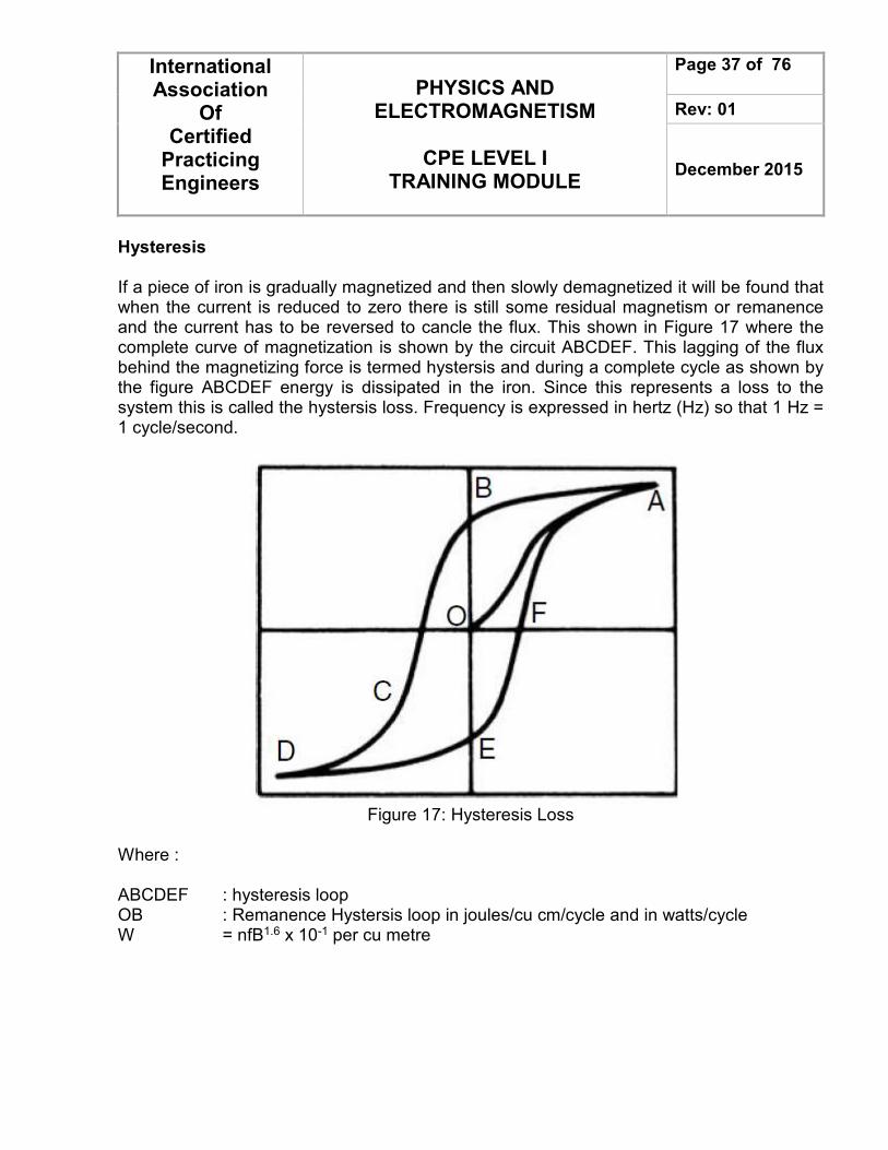
Hysteresis If a piece of iron is gradually magnetized and then slowly demagnetized it will be found that when the current is reduced to zero there is still some residual magnetism or remanence and the current has to be reversed to cancle the flux. This shown in Figure 17 where the complete curve of magnetization is shown by the circuit ABCDEF. This lagging of the flux behind the magnetizing force is termed hystersis and during a complete cycle as shown by the figure ABCDEF energy is dissipated in the iron. Since this represents a loss to the system this is called the hystersis loss. Frequency is expressed in hertz (Hz) so that 1 Hz = 1 cycle/second.
Figure 17: Hysteresis Loss
Where : ABCDEF : hysteresis loop OB : Remanence Hystersis loop in joules/cu cm/cycle and in watts/cycle W = nfB1.6 x 10-1 per cu metre
International Association
Of Certified
Practicing Engineers
PHYSICS AND ELECTROMAGNETISM
CPE LEVEL I
TRAINING MODULE
Page 38 of 76
Rev: 01
December 2015
In an alternating current machine this loss is continuous and its value depends on the materials used.
Watts loss per cubic metre = k1 f n
maxB (12)
Where k1 is a constant for any particular material. The exponent n is known as the Steinmetz or hystersis exponen and is also specific for the material. Originally this was taken as 1.6 but with modern materials working at higher flux densities n can vary from 1.6 to 2.5 or higher. F is the frequency in Hz, and Bmax is the maximum flux-density. Almost all magnetic materials subjected to a cyclic pattern of magnetization around the hystersis loop will also experience the flow of eddy currents which also result in losses. The magnitude of eddy currents can be reduced by increasing the electrical resistance to their flow by making the magnetic circuit of thin laminations and also by the addition of silicon to the iron which increases its resistivity. The silicon also reduces the hystersis loss by reducing the area of the hystersis loop. Eddy current loss is thus given by the expression :
Watts loss per cubic metre = k2 f2 t2 2
effB / ρ (13)
Where k2 is another constant for the material, t the thickness and ρ its resistivity. Beff is the effective flux density which corresponds to its r.m.s. value. When designing electrical machines it is more convenient to relate the magnetic circuit or iron losses to the weight of core iron used rather than its volume. This can be simply done by suitable adjustment of the constants k1 and k2. Typically values of combined hystersis and eddy current losses can be from less than 1 to around 2 W/kg for modern laminations of around 0.3 mm thickness at a flux density of 1.6 tesla and a frequency of 50 Hz.
International Association
Of Certified
Practicing Engineers
PHYSICS AND ELECTROMAGNETISM
CPE LEVEL I
TRAINING MODULE
Page 39 of 76
Rev: 01
December 2015
7. Polarity
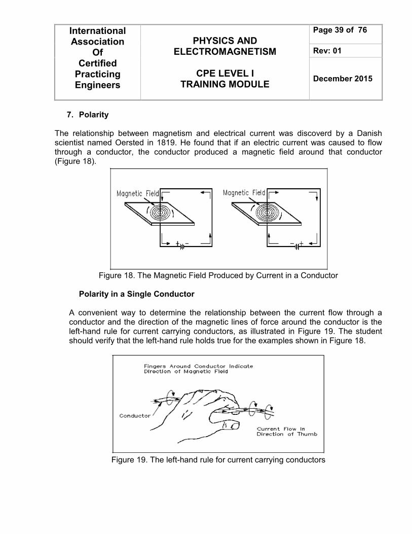
The relationship between magnetism and electrical current was discoverd by a Danish scientist named Oersted in 1819. He found that if an electric current was caused to flow through a conductor, the conductor produced a magnetic field around that conductor (Figure 18).
Figure 18. The Magnetic Field Produced by Current in a Conductor
Polarity in a Single Conductor
A convenient way to determine the relationship between the current flow through a conductor and the direction of the magnetic lines of force around the conductor is the left-hand rule for current carrying conductors, as illustrated in Figure 19. The student should verify that the left-hand rule holds true for the examples shown in Figure 18.
Figure 19. The left-hand rule for current carrying conductors
International Association
Of Certified
Practicing Engineers
PHYSICS AND ELECTROMAGNETISM
CPE LEVEL I
TRAINING MODULE
Page 40 of 76
Rev: 01
December 2015
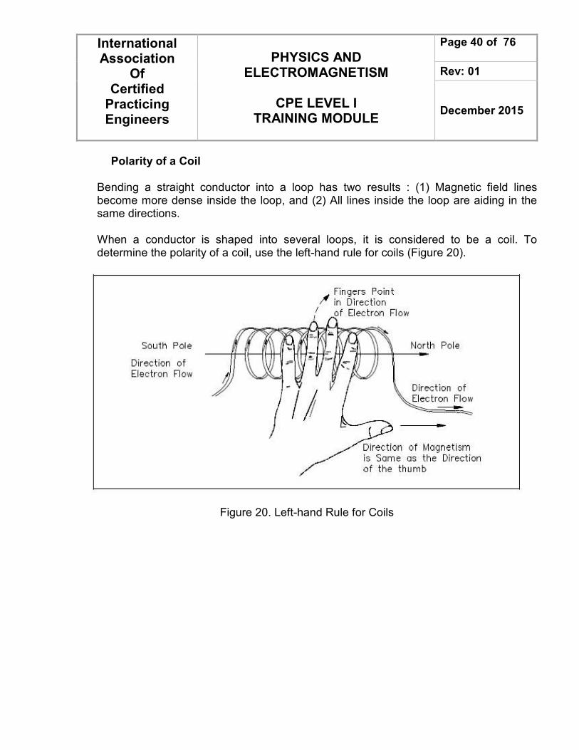
Polarity of a Coil
Bending a straight conductor into a loop has two results : (1) Magnetic field lines become more dense inside the loop, and (2) All lines inside the loop are aiding in the same directions. When a conductor is shaped into several loops, it is considered to be a coil. To determine the polarity of a coil, use the left-hand rule for coils (Figure 20).
Figure 20. Left-hand Rule for Coils
International Association
Of Certified
Practicing Engineers
PHYSICS AND ELECTROMAGNETISM
CPE LEVEL I
TRAINING MODULE
Page 41 of 76
Rev: 01
December 2015
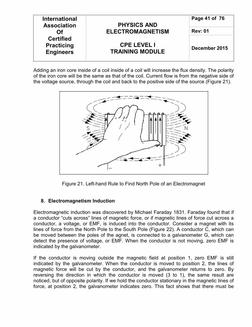
Adding an iron core inside of a coil inside of a coil will increase the flux density. The polarity of the iron core will be the same as that of the coil. Current flow is from the negative side of the voltage source, through the coil and back to the positive side of the source (Figure 21).
Figure 21. Left-hand Rule to Find North Pole of an Electromagnet
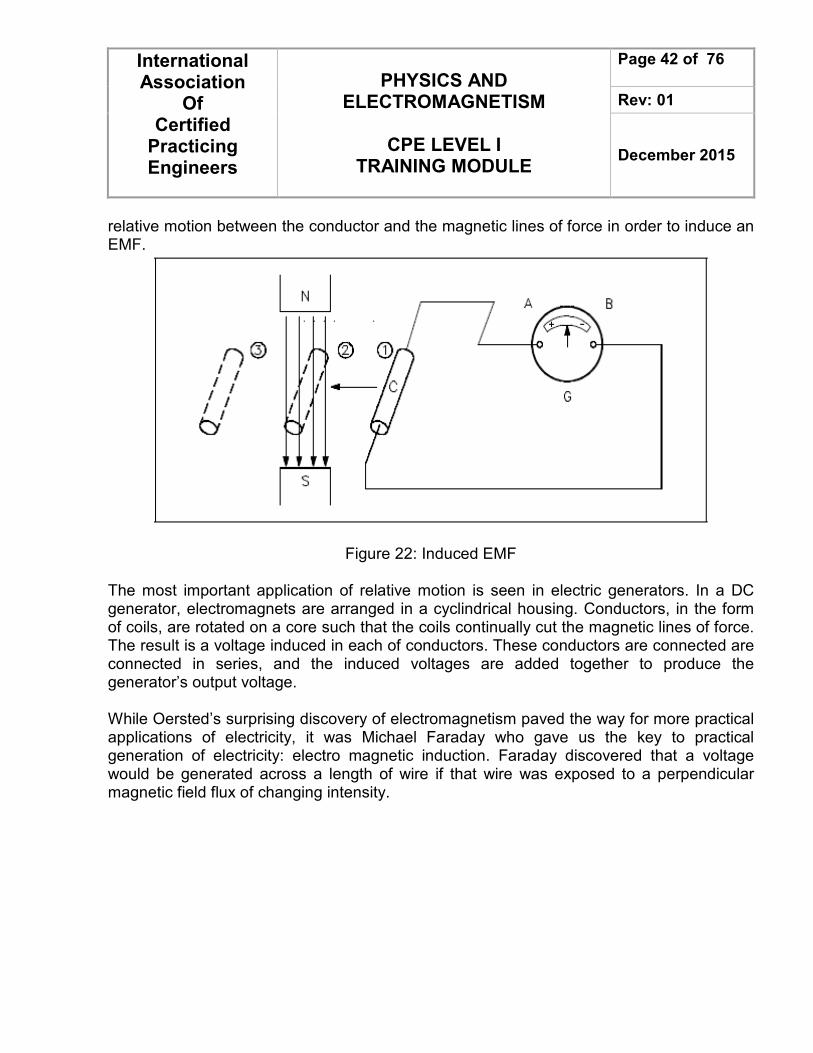
8. Electromagnetism Induction
Electromagnetic induction was discovered by Michael Faraday 1831. Faraday found that if a conductor “cuts across” lines of magnetic force, or if magnetic lines of force cut across a conductor, a voltage, or EMF, is induced into the conductor. Consider a magnet with its lines of force from the North Pole to the South Pole (Figure 22). A conductor C, which can be moved between the poles of the agnet, is connected to a galvanometer G, which can detect the presence of voltage, or EMF. When the conductor is not moving, zero EMF is indicated by the galvanometer.
If the conductor is moving outside the magnetic field at position 1, zero EMF is still indicated by the galvanometer. When the conductor is moved to position 2, the lines of magnetic force will be cut by the conductor, and the galvanometer returns to zero. By reversing the direction in which the conductor is moved (3 to 1), the same result are noticed, but of opposite polarity. If we hold the conductor stationary in the magnetic lines of force, at position 2, the galvanometer indicates zero. This fact shows that there must be
International Association
Of Certified
Practicing Engineers
PHYSICS AND ELECTROMAGNETISM
CPE LEVEL I
TRAINING MODULE
Page 42 of 76
Rev: 01
December 2015
relative motion between the conductor and the magnetic lines of force in order to induce an EMF.
Figure 22: Induced EMF
The most important application of relative motion is seen in electric generators. In a DC generator, electromagnets are arranged in a cyclindrical housing. Conductors, in the form of coils, are rotated on a core such that the coils continually cut the magnetic lines of force. The result is a voltage induced in each of conductors. These conductors are connected are connected in series, and the induced voltages are added together to produce the generator’s output voltage. While Oersted’s surprising discovery of electromagnetism paved the way for more practical applications of electricity, it was Michael Faraday who gave us the key to practical generation of electricity: electro magnetic induction. Faraday discovered that a voltage would be generated across a length of wire if that wire was exposed to a perpendicular magnetic field flux of changing intensity.
International Association
Of Certified
Practicing Engineers
PHYSICS AND ELECTROMAGNETISM
CPE LEVEL I
TRAINING MODULE
Page 43 of 76
Rev: 01
December 2015
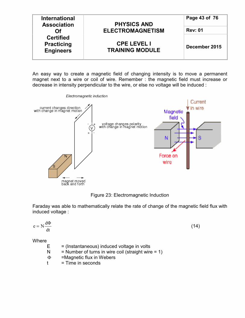
An easy way to create a magnetic field of changing intensity is to move a permanent magnet next to a wire or coil of wire. Remember : the magnetic field must increase or decrease in intensity perpendicular to the wire, or else no voltage will be induced :
Figure 23: Electromagnetic Induction Faraday was able to mathematically relate the rate of change of the magnetic field flux with induced voltage :
dt
dΦNe = (14)
Where E = (Instantaneous) induced voltage in volts N = Number of turns in wire coil (straight wire = 1) Φ =Magnetic flux in Webers t = Time in seconds
International Association
Of Certified
Practicing Engineers
PHYSICS AND ELECTROMAGNETISM
CPE LEVEL I
TRAINING MODULE
Page 44 of 76
Rev: 01
December 2015
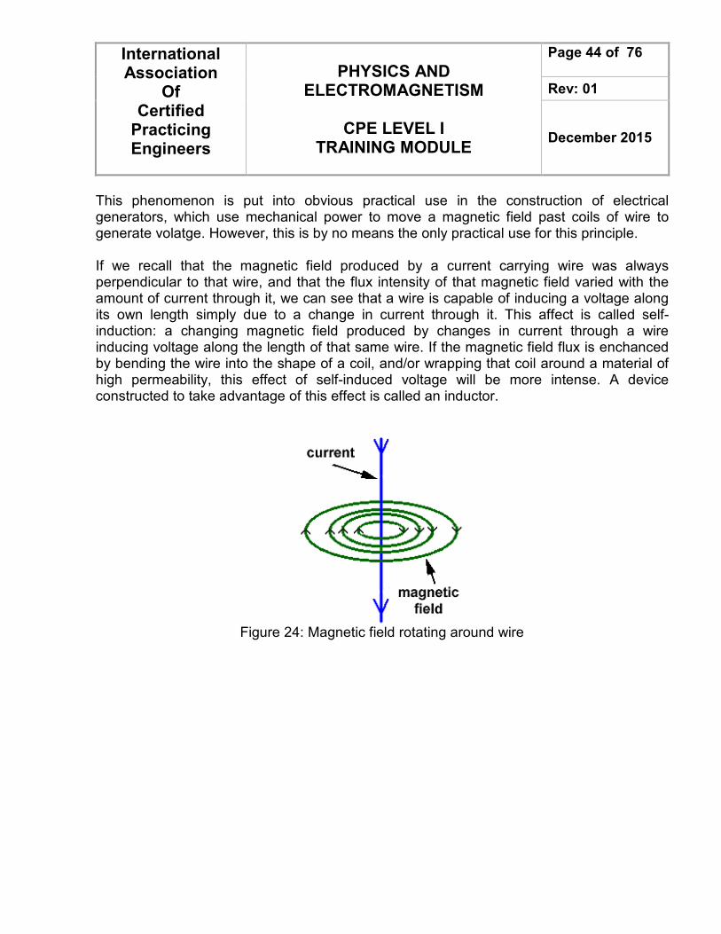
This phenomenon is put into obvious practical use in the construction of electrical generators, which use mechanical power to move a magnetic field past coils of wire to generate volatge. However, this is by no means the only practical use for this principle. If we recall that the magnetic field produced by a current carrying wire was always perpendicular to that wire, and that the flux intensity of that magnetic field varied with the amount of current through it, we can see that a wire is capable of inducing a voltage along its own length simply due to a change in current through it. This affect is called self-induction: a changing magnetic field produced by changes in current through a wire inducing voltage along the length of that same wire. If the magnetic field flux is enchanced by bending the wire into the shape of a coil, and/or wrapping that coil around a material of high permeability, this effect of self-induced voltage will be more intense. A device constructed to take advantage of this effect is called an inductor.
Figure 24: Magnetic field rotating around wire
International Association
Of Certified
Practicing Engineers
PHYSICS AND ELECTROMAGNETISM
CPE LEVEL I
TRAINING MODULE
Page 45 of 76
Rev: 01
December 2015
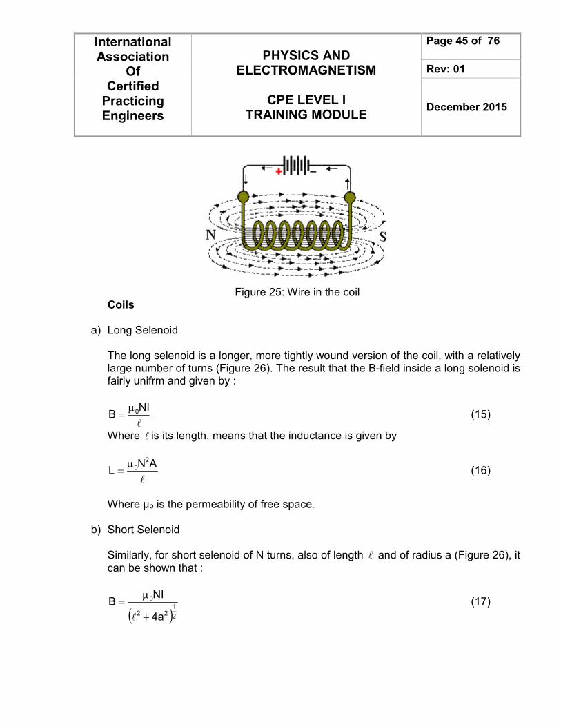
Figure 25: Wire in the coil
Coils
a) Long Selenoid The long selenoid is a longer, more tightly wound version of the coil, with a relatively large number of turns (Figure 26). The result that the B-field inside a long solenoid is fairly unifrm and given by :
l
NIB 0µ= (15)
Where l is its length, means that the inductance is given by
l
ANL
2
0µ= (16)
Where μo is the permeability of free space.
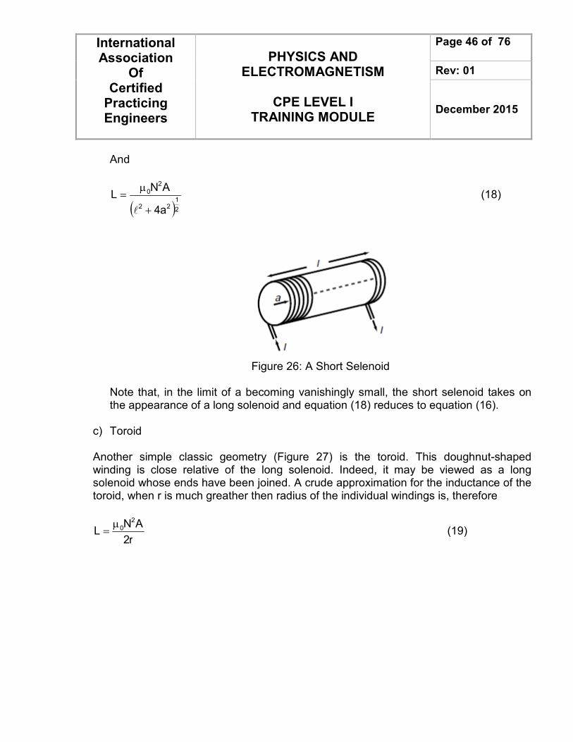
b) Short Selenoid
Similarly, for short selenoid of N turns, also of length l and of radius a (Figure 26), it can be shown that :
( )21
22
0
a4
NIB
+
µ=
l
(17)
International Association
Of Certified
Practicing Engineers
PHYSICS AND ELECTROMAGNETISM
CPE LEVEL I
TRAINING MODULE
Page 46 of 76
Rev: 01
December 2015
And
( )21
22
2
0
a4
ANL
+
µ=
l
(18)
Figure 26: A Short Selenoid
Note that, in the limit of a becoming vanishingly small, the short selenoid takes on the appearance of a long solenoid and equation (18) reduces to equation (16).
c) Toroid Another simple classic geometry (Figure 27) is the toroid. This doughnut-shaped winding is close relative of the long solenoid. Indeed, it may be viewed as a long solenoid whose ends have been joined. A crude approximation for the inductance of the toroid, when r is much greather then radius of the individual windings is, therefore
r2
ANL
2
0µ= (19)
International Association
Of Certified
Practicing Engineers
PHYSICS AND ELECTROMAGNETISM
CPE LEVEL I
TRAINING MODULE
Page 47 of 76
Rev: 01
December 2015
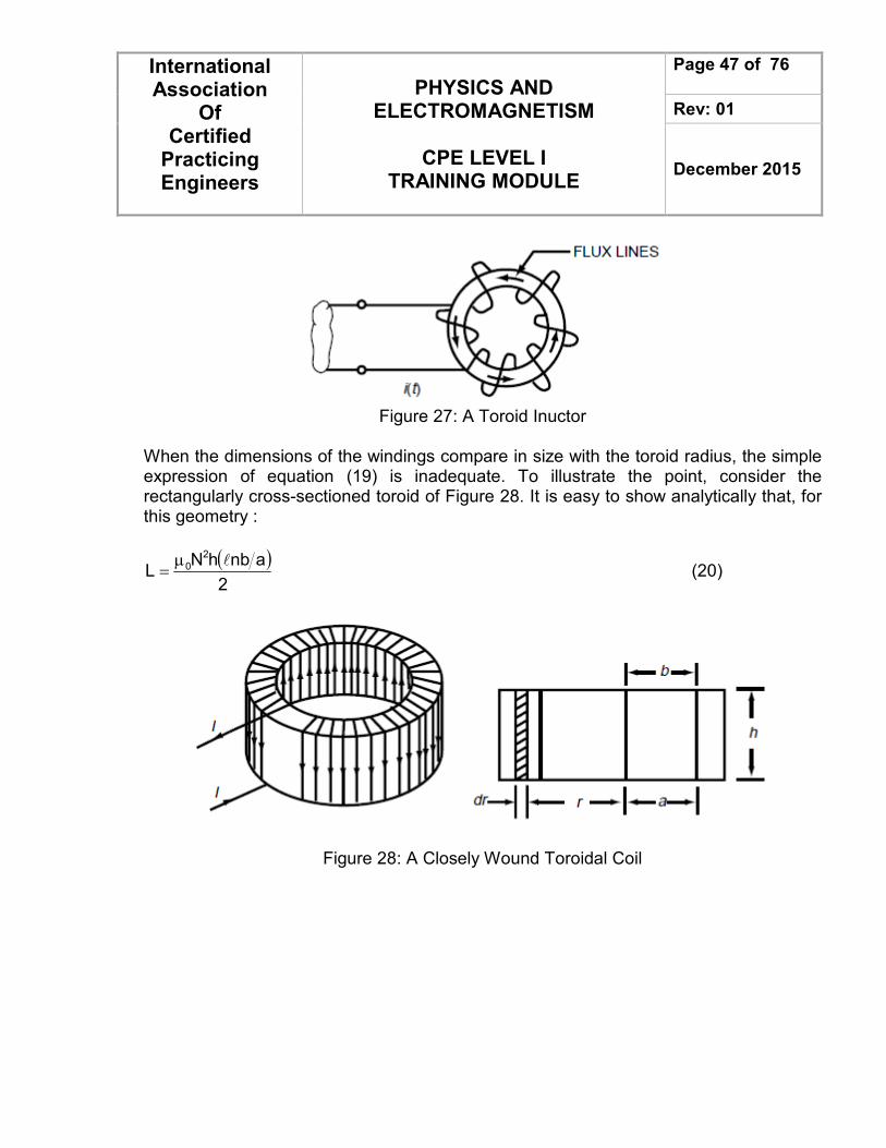
Figure 27: A Toroid Inuctor
When the dimensions of the windings compare in size with the toroid radius, the simple expression of equation (19) is inadequate. To illustrate the point, consider the rectangularly cross-sectioned toroid of Figure 28. It is easy to show analytically that, for this geometry :
( )2
anbhNL
2
0 lµ= (20)
Figure 28: A Closely Wound Toroidal Coil
International Association
Of Certified
Practicing Engineers
PHYSICS AND ELECTROMAGNETISM
CPE LEVEL I
TRAINING MODULE
Page 48 of 76
Rev: 01
December 2015
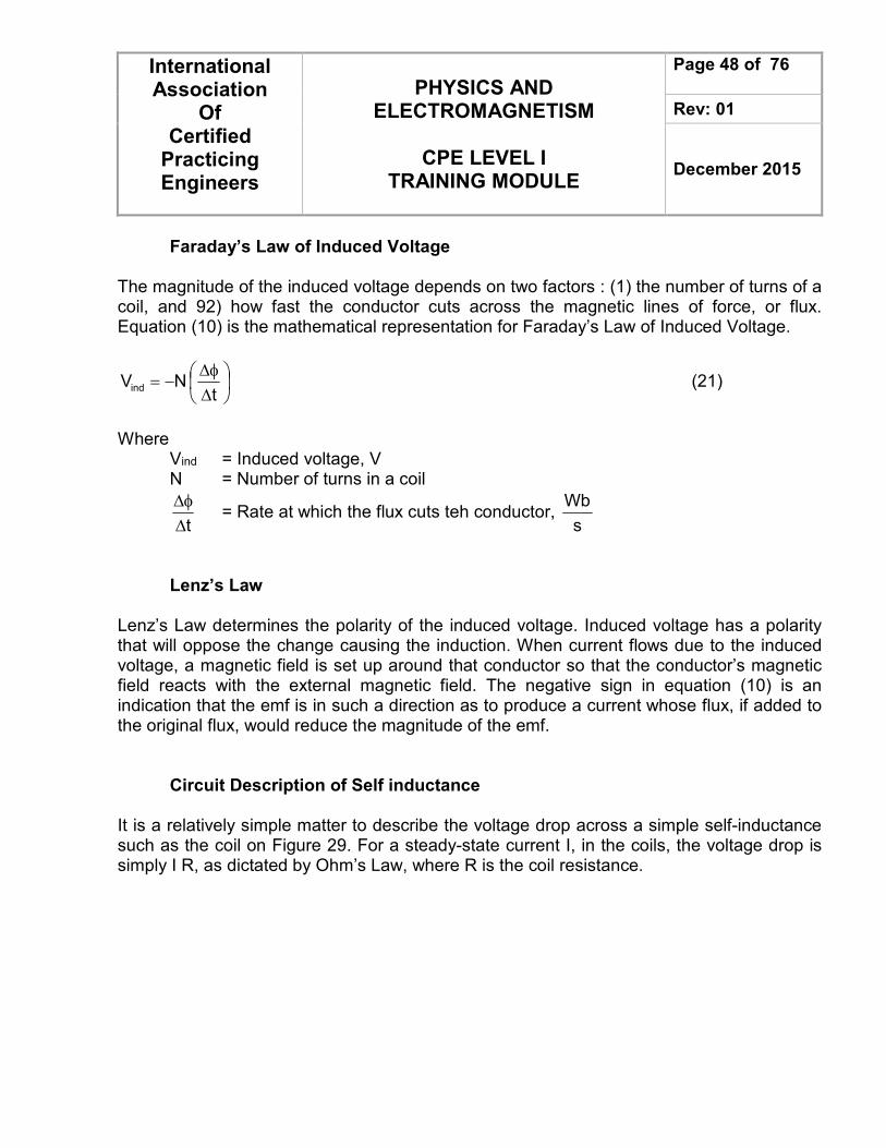
Faraday’s Law of Induced Voltage The magnitude of the induced voltage depends on two factors : (1) the number of turns of a coil, and 92) how fast the conductor cuts across the magnetic lines of force, or flux. Equation (10) is the mathematical representation for Faraday’s Law of Induced Voltage.
∆
φ∆−=
t NVind (21)
Where Vind = Induced voltage, V N = Number of turns in a coil
t∆
φ∆ = Rate at which the flux cuts teh conductor,
s
Wb
Lenz’s Law Lenz’s Law determines the polarity of the induced voltage. Induced voltage has a polarity that will oppose the change causing the induction. When current flows due to the induced voltage, a magnetic field is set up around that conductor so that the conductor’s magnetic field reacts with the external magnetic field. The negative sign in equation (10) is an indication that the emf is in such a direction as to produce a current whose flux, if added to the original flux, would reduce the magnitude of the emf. Circuit Description of Self inductance It is a relatively simple matter to describe the voltage drop across a simple self-inductance such as the coil on Figure 29. For a steady-state current I, in the coils, the voltage drop is simply I R, as dictated by Ohm’s Law, where R is the coil resistance.
International Association
Of Certified
Practicing Engineers
PHYSICS AND ELECTROMAGNETISM
CPE LEVEL I
TRAINING MODULE
Page 49 of 76
Rev: 01
December 2015
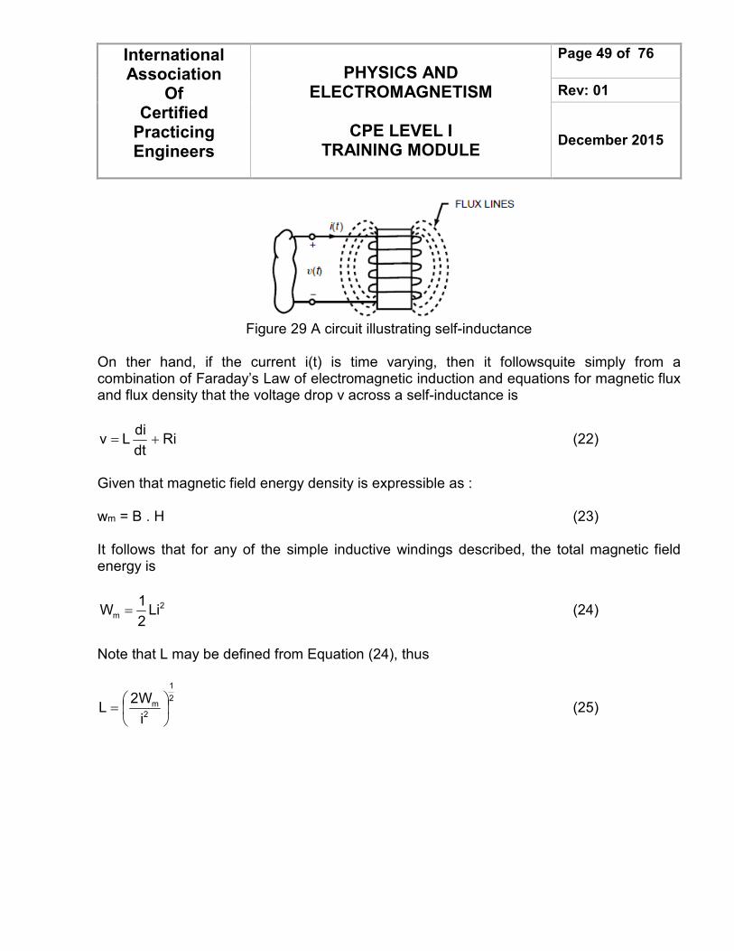
Figure 29 A circuit illustrating self-inductance
On ther hand, if the current i(t) is time varying, then it followsquite simply from a combination of Faraday’s Law of electromagnetic induction and equations for magnetic flux and flux density that the voltage drop v across a self-inductance is
Ridt
diLv += (22)
Given that magnetic field energy density is expressible as : wm = B . H (23) It follows that for any of the simple inductive windings described, the total magnetic field energy is
2
m Li2
1W = (24)
Note that L may be defined from Equation (24), thus
2
1
2
m
i
W2L
= (25)
International Association
Of Certified
Practicing Engineers
PHYSICS AND ELECTROMAGNETISM
CPE LEVEL I
TRAINING MODULE
Page 50 of 76
Rev: 01
December 2015
B. Maxwell Equation
A connection between electricity and magnetism had long been suspected, and in 1820 the Danish physicist Hans Christian Orsted showed that an electric current flowing in a wire produces its own magnetic field. Andre-Marie Ampere of France immediately repeated Orsted's experiments and within weeks was able to express the magnetic forces between current-carrying conductors in a simple and elegant mathematical form. He also demonstrated that a current flowing in a loop of wire produces a magnetic dipole indistinguishable at a distance from that produced by a small permanent magnet; this led Ampere to suggest that magnetism is caused by currents circulating on a molecular scale, an idea remarkably near the modern understanding.
Faraday, in the early 1800's, showed that a changing electric field produces a magnetic field, and that vice-versus, a changing magnetic field produces an electric current. An electromagnet is an iron core which enhances the magnetic field generated by a current flowing through a coil, was invented by William Sturgeon in England during the mid-1820s. It later became a vital component of both motors and generators.
The unification of electric and magnetic phenomena in a complete mathematical theory was the achievement of the Scottish physicist Maxwell (1850's). In a set of four elegant equations, Maxwell formalized the relationship between electric and magnetic fields. In addition, he showed that a linear magnetic and electric field can be self-reinforcing and must move at a particular velocity, the speed of light. Thus, he concluded that light is energy carried in the form of opposite but supporting electric and magnetic fields in the shape of waves, i.e. self-propagating electromagnetic waves.
International Association
Of Certified
Practicing Engineers
PHYSICS AND ELECTROMAGNETISM
CPE LEVEL I
TRAINING MODULE
Page 51 of 76
Rev: 01
December 2015
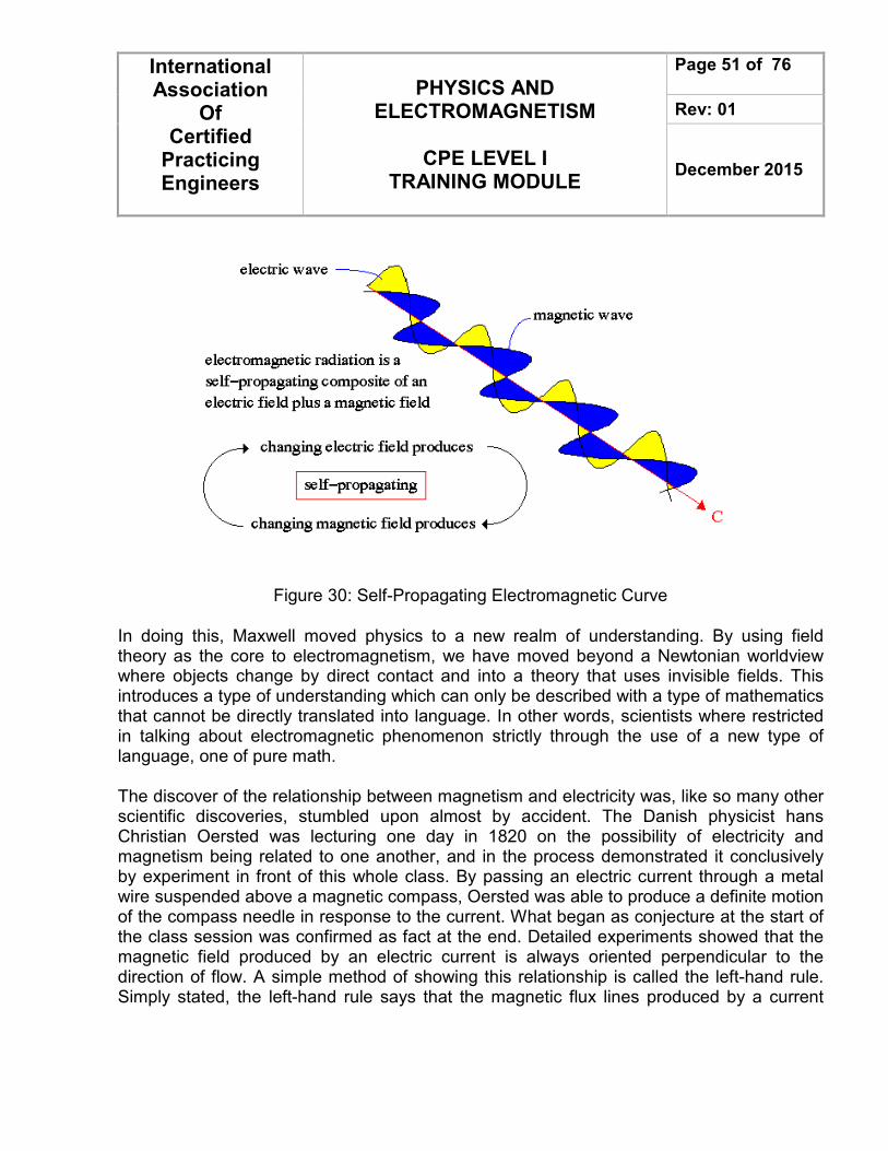
Figure 30: Self-Propagating Electromagnetic Curve
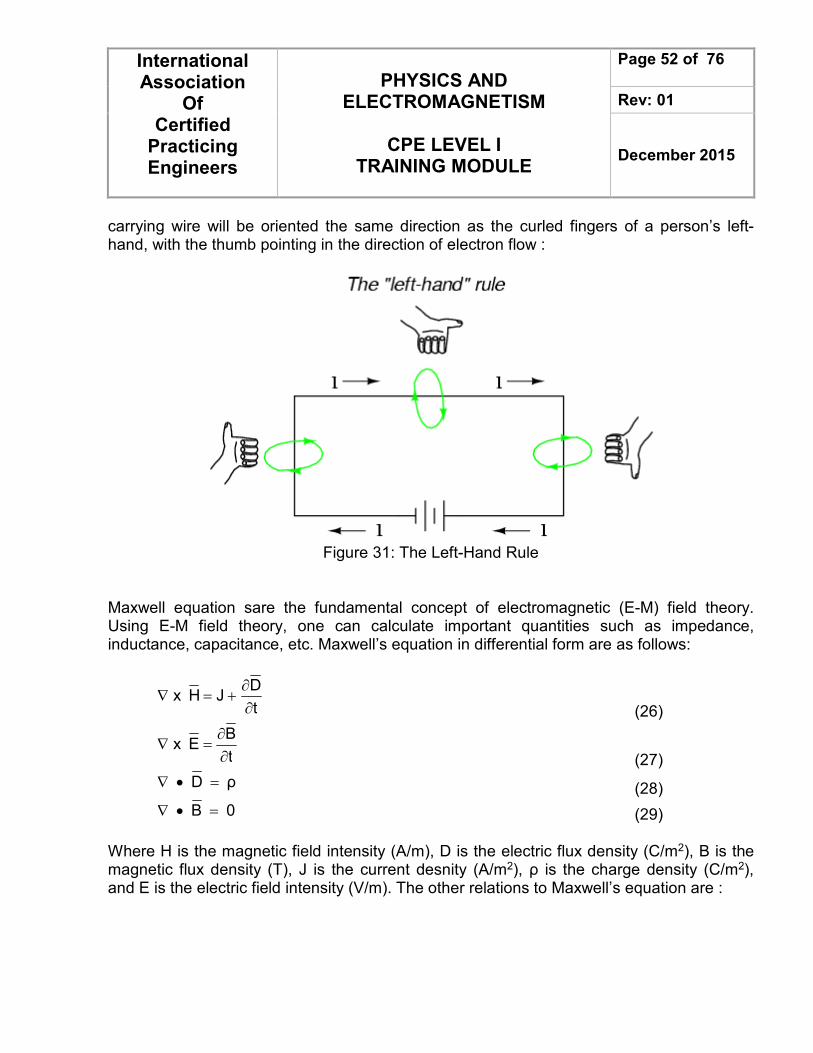
In doing this, Maxwell moved physics to a new realm of understanding. By using field theory as the core to electromagnetism, we have moved beyond a Newtonian worldview where objects change by direct contact and into a theory that uses invisible fields. This introduces a type of understanding which can only be described with a type of mathematics that cannot be directly translated into language. In other words, scientists where restricted in talking about electromagnetic phenomenon strictly through the use of a new type of language, one of pure math. The discover of the relationship between magnetism and electricity was, like so many other scientific discoveries, stumbled upon almost by accident. The Danish physicist hans Christian Oersted was lecturing one day in 1820 on the possibility of electricity and magnetism being related to one another, and in the process demonstrated it conclusively by experiment in front of this whole class. By passing an electric current through a metal wire suspended above a magnetic compass, Oersted was able to produce a definite motion of the compass needle in response to the current. What began as conjecture at the start of the class session was confirmed as fact at the end. Detailed experiments showed that the magnetic field produced by an electric current is always oriented perpendicular to the direction of flow. A simple method of showing this relationship is called the left-hand rule. Simply stated, the left-hand rule says that the magnetic flux lines produced by a current
International Association
Of Certified
Practicing Engineers
PHYSICS AND ELECTROMAGNETISM
CPE LEVEL I
TRAINING MODULE
Page 52 of 76
Rev: 01
December 2015
carrying wire will be oriented the same direction as the curled fingers of a person’s left-hand, with the thumb pointing in the direction of electron flow :
Figure 31: The Left-Hand Rule
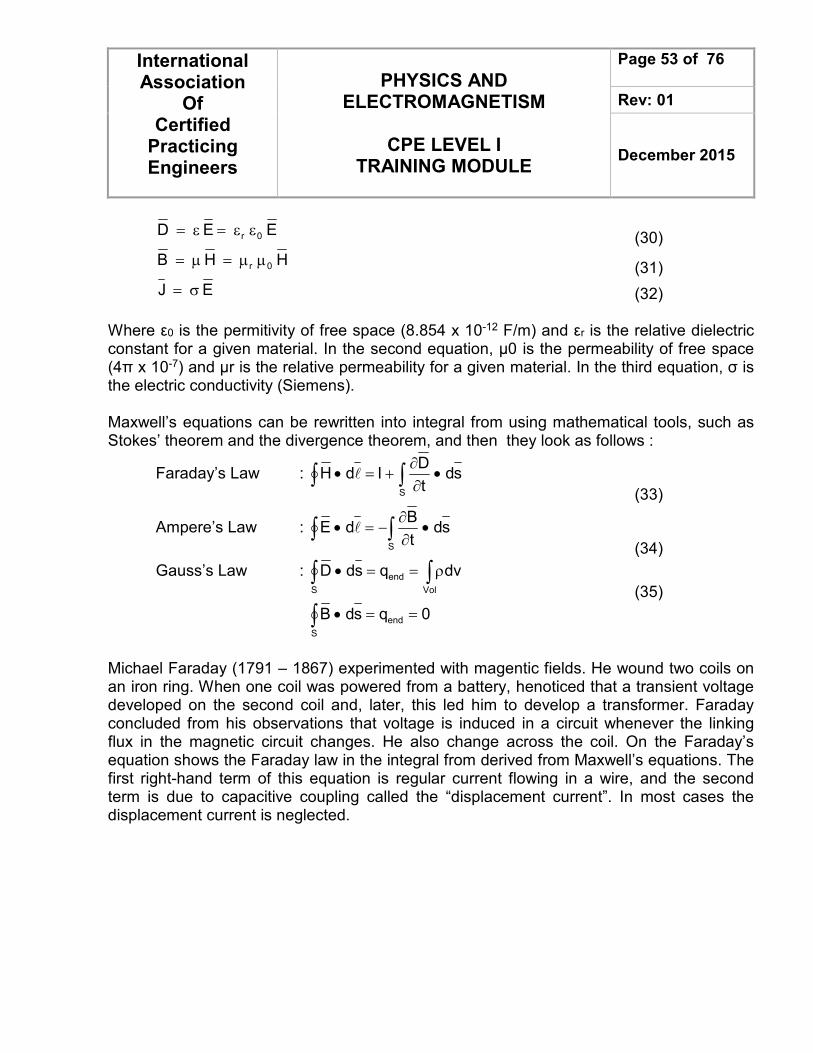
Maxwell equation sare the fundamental concept of electromagnetic (E-M) field theory. Using E-M field theory, one can calculate important quantities such as impedance, inductance, capacitance, etc. Maxwell’s equation in differential form are as follows:
t
DJH x
∂
∂+=∇
(26)
t
BE x
∂
∂=∇
(27)
ρ D =•∇ (28)
0 B =•∇ (29)
Where H is the magnetic field intensity (A/m), D is the electric flux density (C/m2), B is the magnetic flux density (T), J is the current desnity (A/m2), ρ is the charge density (C/m2), and E is the electric field intensity (V/m). The other relations to Maxwell’s equation are :
International Association
Of Certified
Practicing Engineers
PHYSICS AND ELECTROMAGNETISM
CPE LEVEL I
TRAINING MODULE
Page 53 of 76
Rev: 01
December 2015
E E D 0r εε=ε= (30)
H H B 0r µµ=µ= (31)
E J σ= (32)
Where ε0 is the permitivity of free space (8.854 x 10⁻¹² F/m) and εr is the relative dielectric constant for a given material. In the second equation, μ0 is the permeability of free space (4π x 10-7) and μr is the relative permeability for a given material. In the third equation, σ is the electric conductivity (Siemens). Maxwell’s equations can be rewritten into integral from using mathematical tools, such as Stokes’ theorem and the divergence theorem, and then they look as follows :
Faraday’s Law : ∫ ∫ •∂
∂+=•
S
sdt
DIdH l
(33)
Ampere’s Law : ∫ ∫ •∂
∂−=•
S
sdt
BdE l
(34)
Gauss’s Law : ∫ ∫ ρ==•S Vol
end dvqsdD
(35)
0qsdB end
S
==•∫
Michael Faraday (1791 – 1867) experimented with magentic fields. He wound two coils on an iron ring. When one coil was powered from a battery, henoticed that a transient voltage developed on the second coil and, later, this led him to develop a transformer. Faraday concluded from his observations that voltage is induced in a circuit whenever the linking flux in the magnetic circuit changes. He also change across the coil. On the Faraday’s equation shows the Faraday law in the integral from derived from Maxwell’s equations. The first right-hand term of this equation is regular current flowing in a wire, and the second term is due to capacitive coupling called the “displacement current”. In most cases the displacement current is neglected.
International Association
Of Certified
Practicing Engineers
PHYSICS AND ELECTROMAGNETISM
CPE LEVEL I
TRAINING MODULE
Page 54 of 76
Rev: 01
December 2015
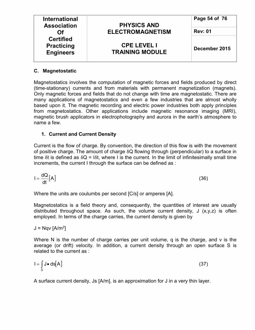
C. Magnetostatic Magnetostatics involves the computation of magnetic forces and fields produced by direct (time-stationary) currents and from materials with permanent magnetization (magnets). Only magnetic forces and fields that do not change with time are magnetostatic. There are many applications of magnetostatics and even a few industries that are almost wholly based upon it. The magnetic recording and electric power industries both apply principles from magnetostatics. Other applications include magnetic resonance imaging (MRI), magnetic brush applicators in electrophotography and aurora in the earth’s atmosphere to name a few.
1. Current and Current Density Current is the flow of charge. By convention, the direction of this flow is with the movement
of positive charge. The amount of charge δQ flowing through (perpendicular) to a surface in time δt is defined as δQ = Iδt, where I is the current. In the limit of infinitesimally small time increments, the current I through the surface can be defined as :
[ ]Adt
dQI = (36)
Where the units are coulumbs per second [C/s] or amperes [A]. Magnetostatics is a field theory and, consequently, the quantities of interest are usually distributed throughout space. As such, the volume current density, J (x,y,z) is often employed. In terms of the charge carries, the current density is given by J = Nqv [A/m2] Where N is the number of charge carries per unit volume, q is the charge, and v is the average (or drift) velocity. In addition, a current density through an open surface S is related to the current as :
[ ]∫ •=S
AdsJI (37)
A surface current density, Js [A/m], is an approximation for J in a very thin layer.
International Association
Of Certified
Practicing Engineers
PHYSICS AND ELECTROMAGNETISM
CPE LEVEL I
TRAINING MODULE
Page 55 of 76
Rev: 01
December 2015
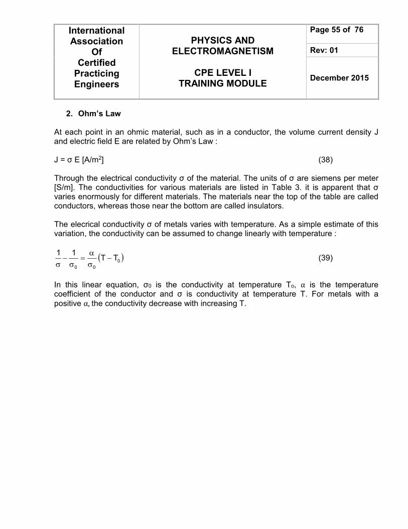
2. Ohm’s Law At each point in an ohmic material, such as in a conductor, the volume current density J and electric field E are related by Ohm’s Law : J = σ E [A/m2] (38) Through the electrical conductivity σ of the material. The units of σ are siemens per meter [S/m]. The conductivities for various materials are listed in Table 3. it is apparent that σ varies enormously for different materials. The materials near the top of the table are called conductors, whereas those near the bottom are called insulators. The elecrical conductivity σ of metals varies with temperature. As a simple estimate of this variation, the conductivity can be assumed to change linearly with temperature :
( )0
00
TT11
−σ
α=
σ−
σ (39)
In this linear equation, σ0 is the conductivity at temperature To, α is the temperature coefficient of the conductor and σ is conductivity at temperature T. For metals with a
positive α, the conductivity decrease with increasing T.
International Association
Of Certified
Practicing Engineers
PHYSICS AND ELECTROMAGNETISM
CPE LEVEL I
TRAINING MODULE
Page 56 of 76
Rev: 01
December 2015
Table 3: Electrical Conductivity σ and Temperature Coefficient α (Near 20oC) for selected Materials at dc.
Material σ (S/m) (20oC) α (per degree Celcius)
Silver Copper (annealed) Gold Aluminium Tungsten Iron (99.98% pure) Tin Constantan Nichrome Carbon (graphite) Seawater Silicon (pure) Distiled water Glass Polystyrene Hard rubber Quartz (fused)
6.29 x 10⁷ 5.8001 x 10⁷
4.10 x 10⁷
3.541 x 10⁷
1.90 x 10⁷
1.0 x x 107
8.70 x 10⁶
2.0 x 10⁶
1.0 x x 106 7.1 x 10⁴
4 4 x 10⁻⁴
≈10-4 ≈10-10 - 10-4
>10-14 ≈10-15 ≈10-16
0.0038 0.00393 0.0034 0.0039 0.0045 0.005
0.0042 0.00001 0.0004 -0.0005
- -0.07
- - - - -
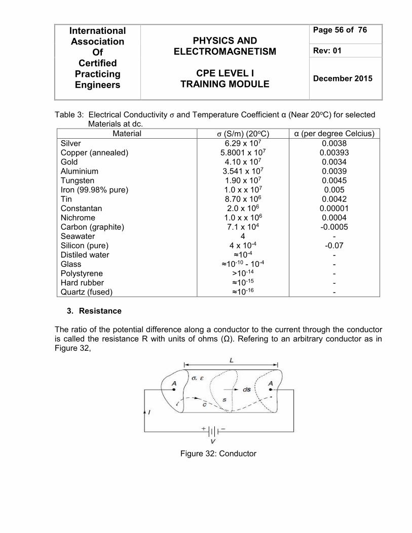
3. Resistance
The ratio of the potential difference along a conductor to the current through the conductor is called the resistance R with units of ohms (Ω). Refering to an arbitrary conductor as in Figure 32,
Figure 32: Conductor
International Association
Of Certified
Practicing Engineers
PHYSICS AND ELECTROMAGNETISM
CPE LEVEL I
TRAINING MODULE
Page 57 of 76
Rev: 01
December 2015
Figure 32 Conventions Used in the Computation of Resistance Using Equation (40) this ratio of voltage to current can be expressed as :
[ ]Ω•σ
•
=•
•
==∫
∫
∫
∫
s
c
s
c
dsE
dlE
dsJ
dlE
I
VR (40)
To conform to the convention that R ≥ 0 for passive conductors, the path of integration c is from the surfaces of higher to lower potential through the conductor, and ds is in the direction of current, as shown in Figure 32. If the conductor in this figure is homogenous with a cross-sectional area A, then from equation (40) :
[ ]Ωσ
=
σ
=A
L
L
VA
V1R (41)
Equation (41) can be used to compute R for any straight, homogenous conductor with a uniform cross-sectional area A at zero frequency. Conversely, if the conductor is inhomogenous or has a nonuniform cross section, R must be computed using equation (40). The resistance R and capacitance C of two perfect conductors (or, simply, two constant potential surfaces) at zero frequency are related as :
σ
ε=RC (42)
Where ε (permitivity) and σ are the material parameters of the otherwise homogenous space between the perfect conductors.
4. Power and Joule’s law Ohm’s law in equation (45) relates the conduction current J to the electric field E at every point in conductive material. Because of collisions between the charge carries (electron s) comprising the current with the lattice of atoms forming the conductive material, there will
International Association
Of Certified
Practicing Engineers
PHYSICS AND ELECTROMAGNETISM
CPE LEVEL I
TRAINING MODULE
Page 58 of 76
Rev: 01
December 2015
be a loss of electrical energy. The power P delivered to electrical charges in a volume v is given by Joule’s law :
[ ]∫ •=v
WJdvEP (43)
Where P has units of joules per second [J/s] or watts [W]. This power is dissipated as heat in the conductive material through an irreversible process since P is unchanged when the direction of E in equation (43) is reversed with J given in equation (1.8). Considering a conductor with a uniform cross section and a length L, if both E and J are directed along the conductor’s length at all points, then from equation (43) :
[ ]WVI
JdsEdlPL s
=
= ∫ ∫ (44)
This familiar expression for power in electrical circuits can be expressed in two alternative forms using Ohm’s law for resistors (in equation 40) as :
[ ]W RIR
VP 2
2
== (45)
This power is dissipated in the resistor and transfered to its surroundings through Joule heating. Conservation of Charge and Kirchhoff’s Current Law A basic postulate of physics is that electrical charge can neither be created nor destroyed. This fact is manifested in electromagnetics through the continuity equation :
tJ
∂
ρ∂−=•∇ (46)
International Association
Of Certified
Practicing Engineers
PHYSICS AND ELECTROMAGNETISM
CPE LEVEL I
TRAINING MODULE
Page 59 of 76
Rev: 01
December 2015
This equation relates the net outward flux of J per unit volume to the time rate of the volume electric charge density ρ at every point. When there is no time variation (which is the situation for magnetostatics), the conservation of charge equation (46) becomes :
0J =•∇ (47)
Physically, this equation tells us that the net outward flux of J per unit volume at every point must vanish. In other words, the electric current density J acts like an incompressible fluid. Applying the divergence theorem, to equation (47) gives the integral form of the static continuity equation as:
∫ =•S
0dsJ (48)
The result is Kirchhoff’s current law (KCL) expressed in integral form. Using equation (49) at a junction of N conducting wires in a nonconducting space (such as air), the currents Ij in all wires satisfy :
∑ =j
j 0I (49)
Which is the circuit form of KCL.
5. Postulates of Magnetostatics The natural phenomenon of magnetostatics is governed by a short and succinct set of equations. The circulation of the magnetic field intensity H [A/m] is governed by Ampere’s law :
JH x =∇ (point form) (50)
∫ =•c
netIdlH (integral form) (51)
The Inet is the net current passing through the open surface bounded by the closed coontour c. Furthermore, the net outward flux of the magnetic flux density B [Wb/m2 or T] is governed by Gauss’s law for magnetic fields :
International Association
Of Certified
Practicing Engineers
PHYSICS AND ELECTROMAGNETISM
CPE LEVEL I
TRAINING MODULE
Page 60 of 76
Rev: 01
December 2015
0B =•∇ (point form) (52)
∫ =•s
0dsB (integral form) (53)
The B and H vector fields are related through the constitutive equation : B = μH [T] (54) Where μ is the permeability [H/m] of the material. All magnetostatic field must satisfy the equation (50) therough (54). Very few magnetostatic problems, however, have simple and analytical solutions for the vector fields B and H. Biot-Savart Law and Vector Magnetic Potential A Amperes’s law (equations 50 and 51) and Gauss’s law (equations 52 and 53) are the rules that all magnetostatic fields must obey. Except in very limited situations, these laws cannot be used to directly compute B or H. Instead, if a given current density J is prescribed at source coordinates r’, the B field can be directly computed at any observation coordinate r using the Biot-Savart law.
( ) ( ) [ ]∫πµ
='r
3T'dv
R
R x 'rJ
4rB (55)
The vector R = r – r’ points from the source point to the observation point. For a surface current density Js, the Biot-Savart law reads :
( ) ( ) [ ]∫πµ
='s
3
s T'dsR
R x 'rJ
4rB (56)
Whereas for a filamentary current I (pointing in the direction of dl’ at r’), the Biot-Savart law is written as:
( ) ( ) [ ]∫πµ
='c
3T
R
R x dl''rI
4rB (57)
International Association
Of Certified
Practicing Engineers
PHYSICS AND ELECTROMAGNETISM
CPE LEVEL I
TRAINING MODULE
Page 61 of 76
Rev: 01
December 2015
The B field can also be computed from the magnetic vector potential A as:
[ ]T A x B ∇= (58)
Where for a volume current density J at source coordinates r’:
( ) ( ) [ ]∫πµ
='v
m/Wb 'dvR
'rJ
4rA (59)
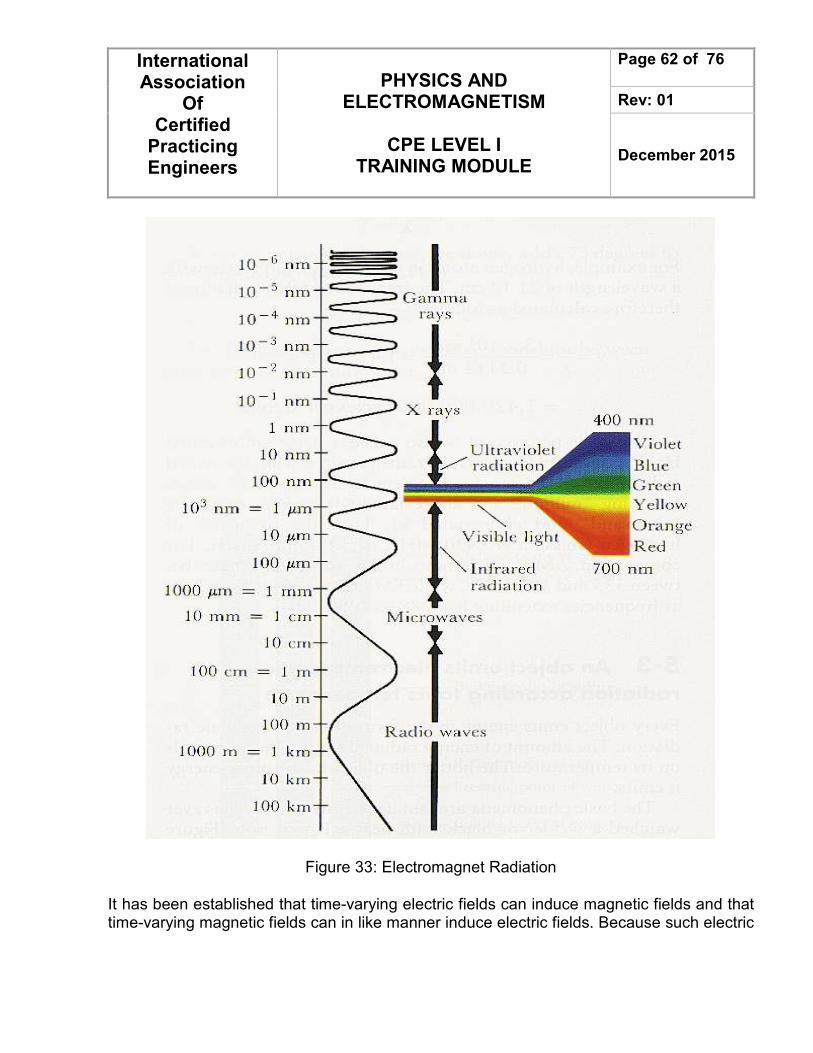
D. Electromagnet Radiation The electromagnetic (EM) spectrum consists of all forms of EM radiation, for example, EM waves propagating through space, from direct current (DC) to light to gamma rays. The EM spectrum can be arranged inorder of frequency or wavelength into a number of regions, usually wide in extent, within which the EM waves have some specified common characteristics, for example, those charachteristics relating to the production or detection of radiation. Electromagnetic radiation is energy that is propagated through free space or through a material medium in the form of electromagnetic waves, such as radio waves, visible light, and gamma rays. The term also refers to the emission and transmission of such radiant energy.
The wavelength of the light determines its characteristics. For example, short wavelengths are high energy gamma-rays and x-rays, long wavelengths are radio waves. The whole range of wavelengths is called the electromagnetic spectrum.
In 1887 Heinrich Hertz, a German physicist, provided experimental confirmation of Maxwell's ideas by producing the first man-made electromagnetic waves and investigating their properties. Subsequent studies resulted in a broader understanding of the nature and origin of radiant energy.
International Association
Of Certified
Practicing Engineers
PHYSICS AND ELECTROMAGNETISM
CPE LEVEL I
TRAINING MODULE
Page 62 of 76
Rev: 01
December 2015
Figure 33: Electromagnet Radiation
It has been established that time-varying electric fields can induce magnetic fields and that time-varying magnetic fields can in like manner induce electric fields. Because such electric
International Association
Of Certified
Practicing Engineers
PHYSICS AND ELECTROMAGNETISM
CPE LEVEL I
TRAINING MODULE
Page 63 of 76
Rev: 01
December 2015
and magnetic fields generate each other, they occur jointly, and together they propagate as electromagnetic waves. An electromagnetic wave is a transverse wave in that the electric field and the magnetic field at any point and time in the wave are perpendicular to each other as well as to the direction of propagation. In free space (i.e., a space that is absolutely devoid of matter and that experiences no intrusion from other fields or forces), electromagnetic waves always propagate with the same speed--that of light (299,792,458 m per second, or 186,282 miles per second)--independent of the speed of the observer or of the source of the waves.
Electromagnetic radiation has properties in common with other forms of waves such as reflection, refraction, diffraction, and interference. Moreover, it may be characterized by the frequency with which it varies over time or by its wavelength. Electromagnetic radiation, however, has particle-like properties in addition to those associated with wave motion. It is quantized in that for a given frequency, its energy occurs as an integer times h, in which h is a fundamental constant of nature known as Planck's constant. A quantum of electromagnetic energy is called a photon. Visible light and other forms of electromagnetic radiation may be thought of as a stream of photons, with photon energy directly proportional to frequency.
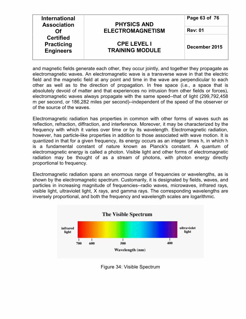
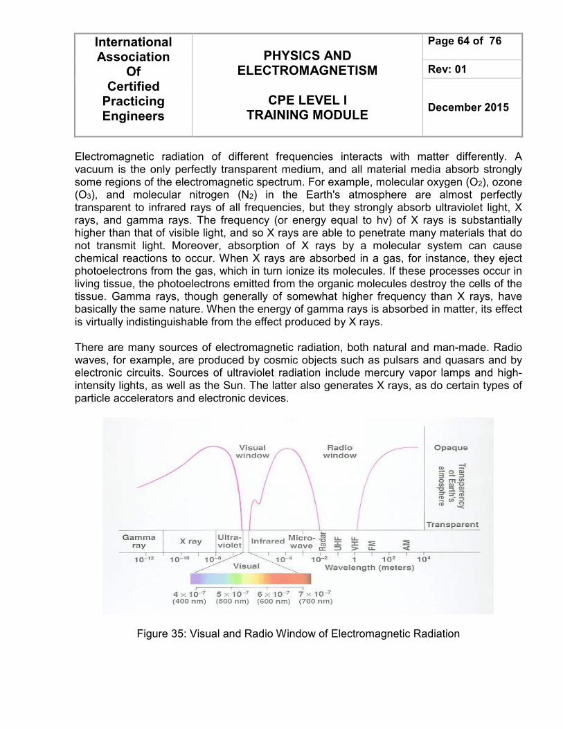
Electromagnetic radiation spans an enormous range of frequencies or wavelengths, as is shown by the electromagnetic spectrum. Customarily, it is designated by fields, waves, and particles in increasing magnitude of frequencies--radio waves, microwaves, infrared rays, visible light, ultraviolet light, X rays, and gamma rays. The corresponding wavelengths are inversely proportional, and both the frequency and wavelength scales are logarithmic.
Figure 34: Visible Spectrum
International Association
Of Certified
Practicing Engineers
PHYSICS AND ELECTROMAGNETISM
CPE LEVEL I
TRAINING MODULE
Page 64 of 76
Rev: 01
December 2015
Electromagnetic radiation of different frequencies interacts with matter differently. A vacuum is the only perfectly transparent medium, and all material media absorb strongly some regions of the electromagnetic spectrum. For example, molecular oxygen (O2), ozone (O3), and molecular nitrogen (N2) in the Earth's atmosphere are almost perfectly transparent to infrared rays of all frequencies, but they strongly absorb ultraviolet light, X rays, and gamma rays. The frequency (or energy equal to hv) of X rays is substantially higher than that of visible light, and so X rays are able to penetrate many materials that do not transmit light. Moreover, absorption of X rays by a molecular system can cause chemical reactions to occur. When X rays are absorbed in a gas, for instance, they eject photoelectrons from the gas, which in turn ionize its molecules. If these processes occur in living tissue, the photoelectrons emitted from the organic molecules destroy the cells of the tissue. Gamma rays, though generally of somewhat higher frequency than X rays, have basically the same nature. When the energy of gamma rays is absorbed in matter, its effect is virtually indistinguishable from the effect produced by X rays.
There are many sources of electromagnetic radiation, both natural and man-made. Radio waves, for example, are produced by cosmic objects such as pulsars and quasars and by electronic circuits. Sources of ultraviolet radiation include mercury vapor lamps and high-intensity lights, as well as the Sun. The latter also generates X rays, as do certain types of particle accelerators and electronic devices.
Figure 35: Visual and Radio Window of Electromagnetic Radiation
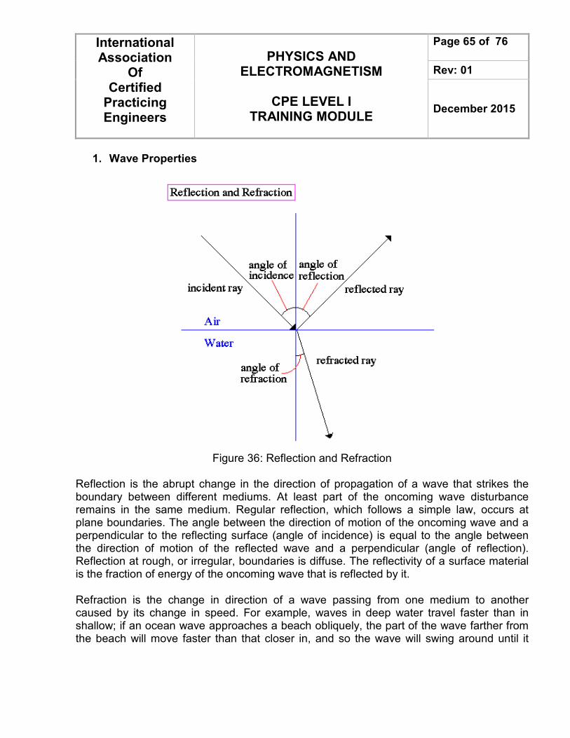
International Association
Of Certified
Practicing Engineers
PHYSICS AND ELECTROMAGNETISM
CPE LEVEL I
TRAINING MODULE
Page 65 of 76
Rev: 01
December 2015
1. Wave Properties
Figure 36: Reflection and Refraction
Reflection is the abrupt change in the direction of propagation of a wave that strikes the boundary between different mediums. At least part of the oncoming wave disturbance remains in the same medium. Regular reflection, which follows a simple law, occurs at plane boundaries. The angle between the direction of motion of the oncoming wave and a perpendicular to the reflecting surface (angle of incidence) is equal to the angle between the direction of motion of the reflected wave and a perpendicular (angle of reflection). Reflection at rough, or irregular, boundaries is diffuse. The reflectivity of a surface material is the fraction of energy of the oncoming wave that is reflected by it.
Refraction is the change in direction of a wave passing from one medium to another caused by its change in speed. For example, waves in deep water travel faster than in shallow; if an ocean wave approaches a beach obliquely, the part of the wave farther from the beach will move faster than that closer in, and so the wave will swing around until it
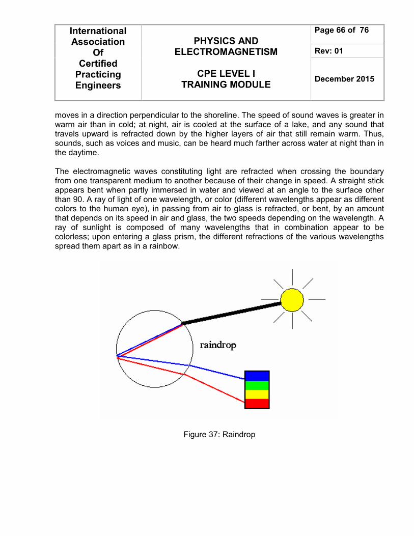
International Association
Of Certified
Practicing Engineers
PHYSICS AND ELECTROMAGNETISM
CPE LEVEL I
TRAINING MODULE
Page 66 of 76
Rev: 01
December 2015
moves in a direction perpendicular to the shoreline. The speed of sound waves is greater in warm air than in cold; at night, air is cooled at the surface of a lake, and any sound that travels upward is refracted down by the higher layers of air that still remain warm. Thus, sounds, such as voices and music, can be heard much farther across water at night than in the daytime.
The electromagnetic waves constituting light are refracted when crossing the boundary from one transparent medium to another because of their change in speed. A straight stick appears bent when partly immersed in water and viewed at an angle to the surface other than 90. A ray of light of one wavelength, or color (different wavelengths appear as different colors to the human eye), in passing from air to glass is refracted, or bent, by an amount that depends on its speed in air and glass, the two speeds depending on the wavelength. A ray of sunlight is composed of many wavelengths that in combination appear to be colorless; upon entering a glass prism, the different refractions of the various wavelengths spread them apart as in a rainbow.
Figure 37: Raindrop
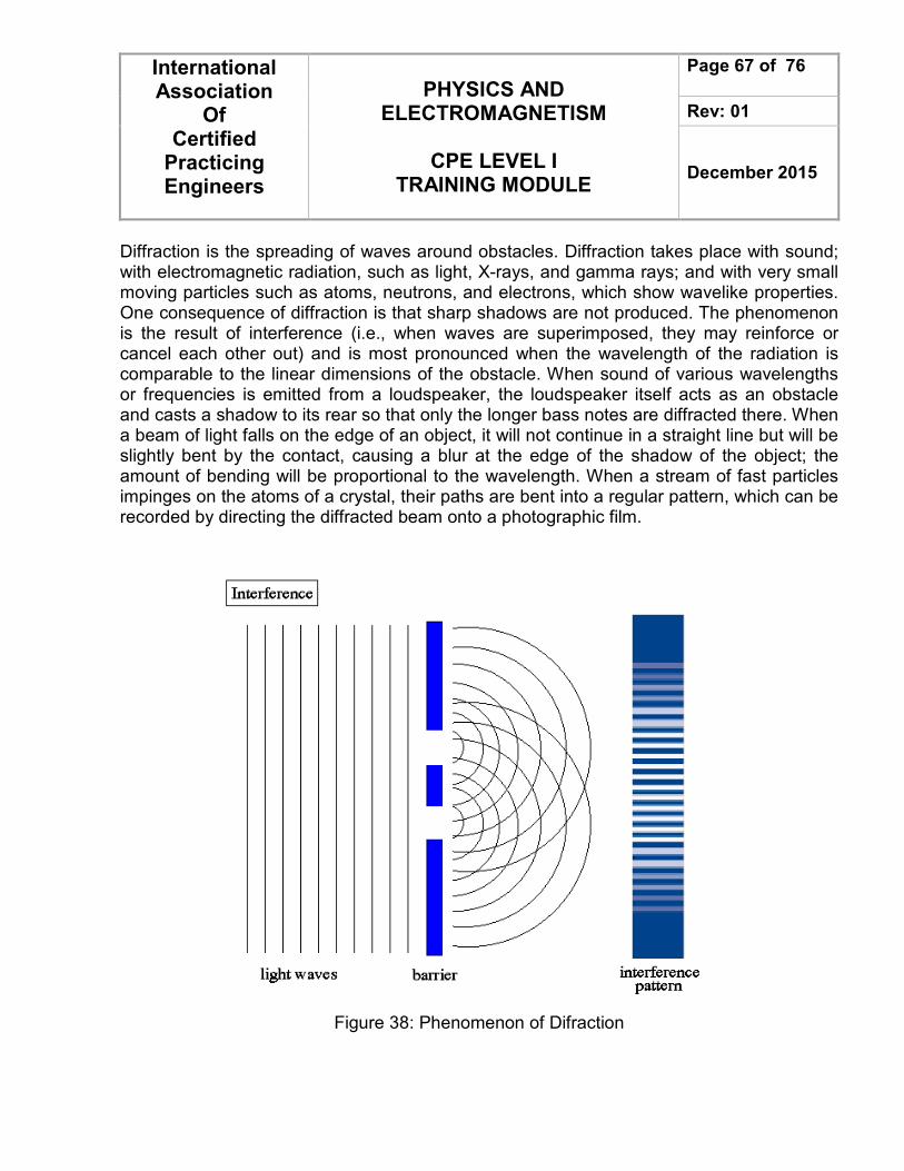
International Association
Of Certified
Practicing Engineers
PHYSICS AND ELECTROMAGNETISM
CPE LEVEL I
TRAINING MODULE
Page 67 of 76
Rev: 01
December 2015
Diffraction is the spreading of waves around obstacles. Diffraction takes place with sound; with electromagnetic radiation, such as light, X-rays, and gamma rays; and with very small moving particles such as atoms, neutrons, and electrons, which show wavelike properties. One consequence of diffraction is that sharp shadows are not produced. The phenomenon is the result of interference (i.e., when waves are superimposed, they may reinforce or cancel each other out) and is most pronounced when the wavelength of the radiation is comparable to the linear dimensions of the obstacle. When sound of various wavelengths or frequencies is emitted from a loudspeaker, the loudspeaker itself acts as an obstacle and casts a shadow to its rear so that only the longer bass notes are diffracted there. When a beam of light falls on the edge of an object, it will not continue in a straight line but will be slightly bent by the contact, causing a blur at the edge of the shadow of the object; the amount of bending will be proportional to the wavelength. When a stream of fast particles impinges on the atoms of a crystal, their paths are bent into a regular pattern, which can be recorded by directing the diffracted beam onto a photographic film.
Figure 38: Phenomenon of Difraction
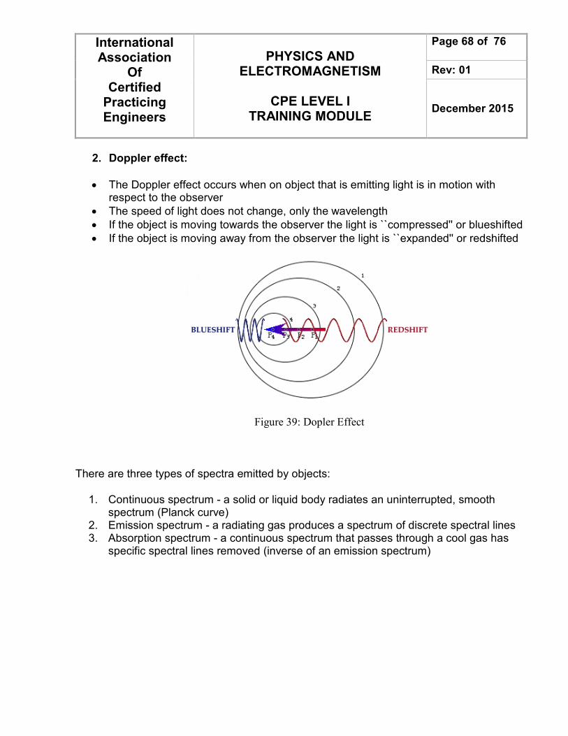
International Association
Of Certified
Practicing Engineers
PHYSICS AND ELECTROMAGNETISM
CPE LEVEL I
TRAINING MODULE
Page 68 of 76
Rev: 01
December 2015
2. Doppler effect:
• The Doppler effect occurs when on object that is emitting light is in motion with respect to the observer
• The speed of light does not change, only the wavelength
• If the object is moving towards the observer the light is ``compressed'' or blueshifted
• If the object is moving away from the observer the light is ``expanded'' or redshifted
Figure 39: Dopler Effect
There are three types of spectra emitted by objects:
1. Continuous spectrum - a solid or liquid body radiates an uninterrupted, smooth spectrum (Planck curve)
2. Emission spectrum - a radiating gas produces a spectrum of discrete spectral lines 3. Absorption spectrum - a continuous spectrum that passes through a cool gas has
specific spectral lines removed (inverse of an emission spectrum)
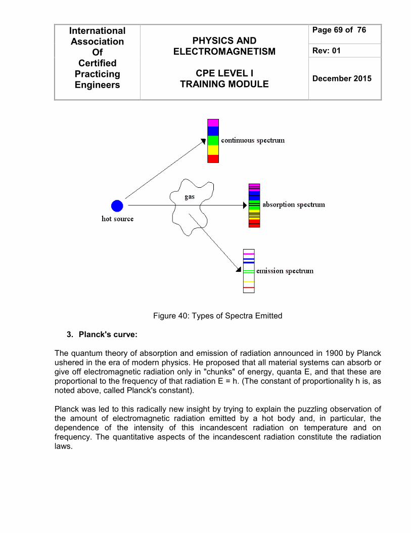
International Association
Of Certified
Practicing Engineers
PHYSICS AND ELECTROMAGNETISM
CPE LEVEL I
TRAINING MODULE
Page 69 of 76
Rev: 01
December 2015
Figure 40: Types of Spectra Emitted
3. Planck's curve:
The quantum theory of absorption and emission of radiation announced in 1900 by Planck ushered in the era of modern physics. He proposed that all material systems can absorb or give off electromagnetic radiation only in "chunks" of energy, quanta E, and that these are proportional to the frequency of that radiation E = h. (The constant of proportionality h is, as noted above, called Planck's constant).
Planck was led to this radically new insight by trying to explain the puzzling observation of the amount of electromagnetic radiation emitted by a hot body and, in particular, the dependence of the intensity of this incandescent radiation on temperature and on frequency. The quantitative aspects of the incandescent radiation constitute the radiation laws.
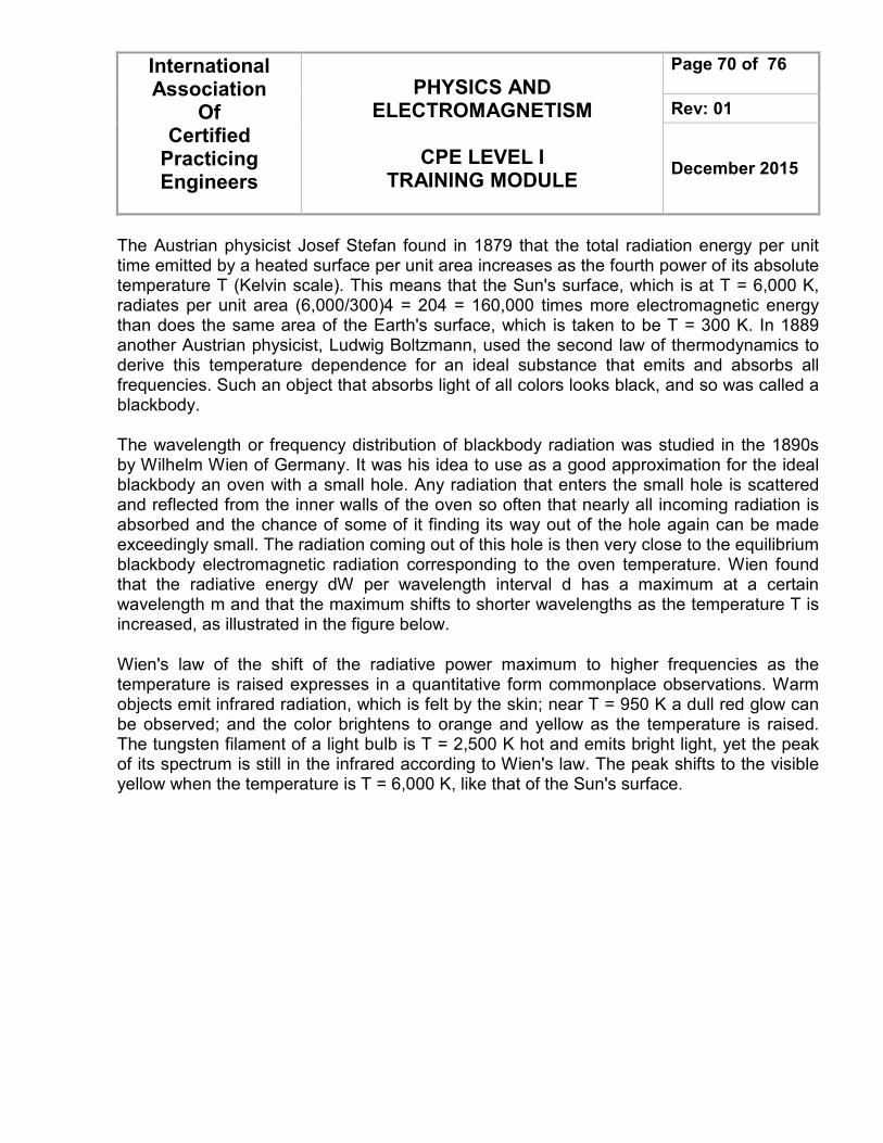
International Association
Of Certified
Practicing Engineers
PHYSICS AND ELECTROMAGNETISM
CPE LEVEL I
TRAINING MODULE
Page 70 of 76
Rev: 01
December 2015
The Austrian physicist Josef Stefan found in 1879 that the total radiation energy per unit time emitted by a heated surface per unit area increases as the fourth power of its absolute temperature T (Kelvin scale). This means that the Sun's surface, which is at T = 6,000 K, radiates per unit area (6,000/300)4 = 204 = 160,000 times more electromagnetic energy than does the same area of the Earth's surface, which is taken to be T = 300 K. In 1889 another Austrian physicist, Ludwig Boltzmann, used the second law of thermodynamics to derive this temperature dependence for an ideal substance that emits and absorbs all frequencies. Such an object that absorbs light of all colors looks black, and so was called a blackbody.
The wavelength or frequency distribution of blackbody radiation was studied in the 1890s by Wilhelm Wien of Germany. It was his idea to use as a good approximation for the ideal blackbody an oven with a small hole. Any radiation that enters the small hole is scattered and reflected from the inner walls of the oven so often that nearly all incoming radiation is absorbed and the chance of some of it finding its way out of the hole again can be made exceedingly small. The radiation coming out of this hole is then very close to the equilibrium blackbody electromagnetic radiation corresponding to the oven temperature. Wien found that the radiative energy dW per wavelength interval d has a maximum at a certain wavelength m and that the maximum shifts to shorter wavelengths as the temperature T is increased, as illustrated in the figure below.
Wien's law of the shift of the radiative power maximum to higher frequencies as the temperature is raised expresses in a quantitative form commonplace observations. Warm objects emit infrared radiation, which is felt by the skin; near T = 950 K a dull red glow can be observed; and the color brightens to orange and yellow as the temperature is raised. The tungsten filament of a light bulb is T = 2,500 K hot and emits bright light, yet the peak of its spectrum is still in the infrared according to Wien's law. The peak shifts to the visible yellow when the temperature is T = 6,000 K, like that of the Sun's surface.
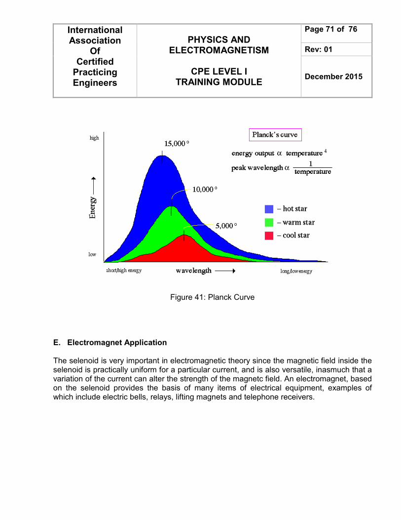
International Association
Of Certified
Practicing Engineers
PHYSICS AND ELECTROMAGNETISM
CPE LEVEL I
TRAINING MODULE
Page 71 of 76
Rev: 01
December 2015
Figure 41: Planck Curve
E. Electromagnet Application
The selenoid is very important in electromagnetic theory since the magnetic field inside the selenoid is practically uniform for a particular current, and is also versatile, inasmuch that a variation of the current can alter the strength of the magnetc field. An electromagnet, based on the selenoid provides the basis of many items of electrical equipment, examples of which include electric bells, relays, lifting magnets and telephone receivers.
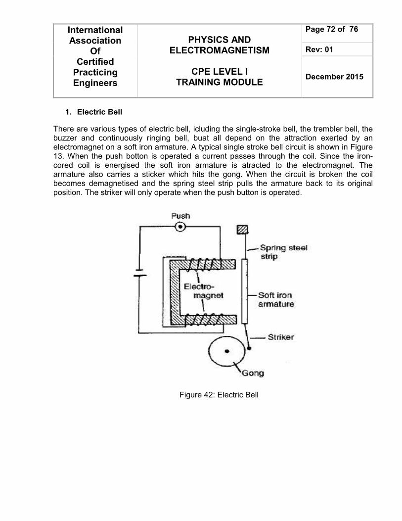
International Association
Of Certified
Practicing Engineers
PHYSICS AND ELECTROMAGNETISM
CPE LEVEL I
TRAINING MODULE
Page 72 of 76
Rev: 01
December 2015
1. Electric Bell
There are various types of electric bell, icluding the single-stroke bell, the trembler bell, the buzzer and continuously ringing bell, buat all depend on the attraction exerted by an electromagnet on a soft iron armature. A typical single stroke bell circuit is shown in Figure 13. When the push botton is operated a current passes through the coil. Since the iron-cored coil is energised the soft iron armature is atracted to the electromagnet. The armature also carries a sticker which hits the gong. When the circuit is broken the coil becomes demagnetised and the spring steel strip pulls the armature back to its original position. The striker will only operate when the push button is operated.
Figure 42: Electric Bell
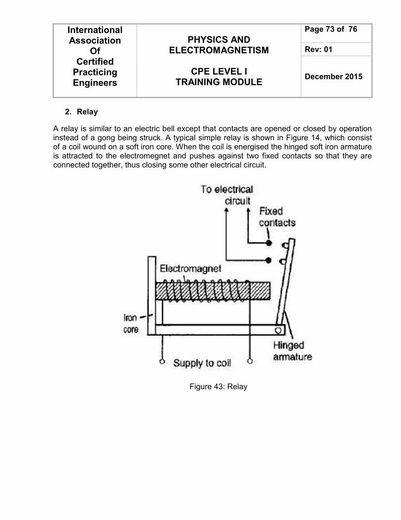
International Association
Of Certified
Practicing Engineers
PHYSICS AND ELECTROMAGNETISM
CPE LEVEL I
TRAINING MODULE
Page 73 of 76
Rev: 01
December 2015
2. Relay
A relay is similar to an electric bell except that contacts are opened or closed by operation instead of a gong being struck. A typical simple relay is shown in Figure 14, which consist of a coil wound on a soft iron core. When the coil is energised the hinged soft iron armature is attracted to the electromegnet and pushes against two fixed contacts so that they are connected together, thus closing some other electrical circuit.
Figure 43: Relay
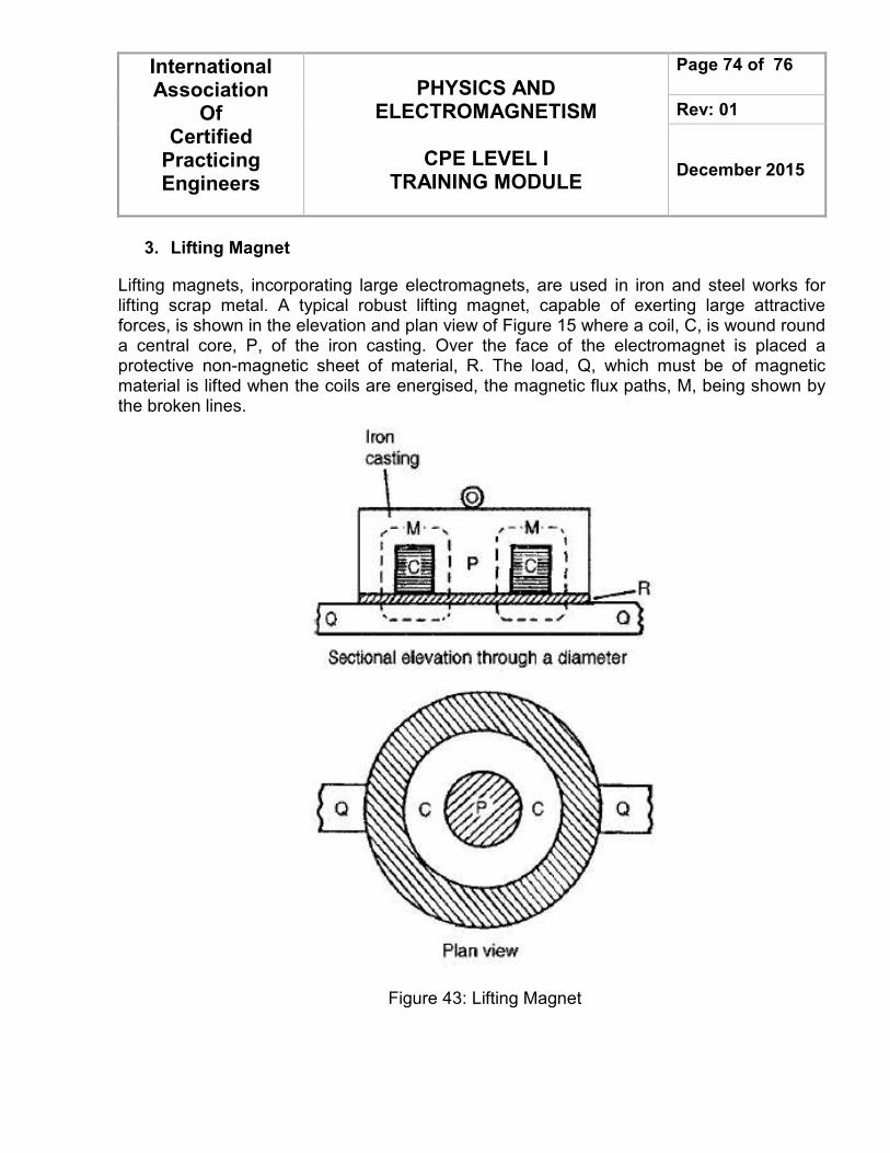
International Association
Of Certified
Practicing Engineers
PHYSICS AND ELECTROMAGNETISM
CPE LEVEL I
TRAINING MODULE
Page 74 of 76
Rev: 01
December 2015
3. Lifting Magnet
Lifting magnets, incorporating large electromagnets, are used in iron and steel works for lifting scrap metal. A typical robust lifting magnet, capable of exerting large attractive forces, is shown in the elevation and plan view of Figure 15 where a coil, C, is wound round a central core, P, of the iron casting. Over the face of the electromagnet is placed a protective non-magnetic sheet of material, R. The load, Q, which must be of magnetic material is lifted when the coils are energised, the magnetic flux paths, M, being shown by the broken lines.
Figure 43: Lifting Magnet
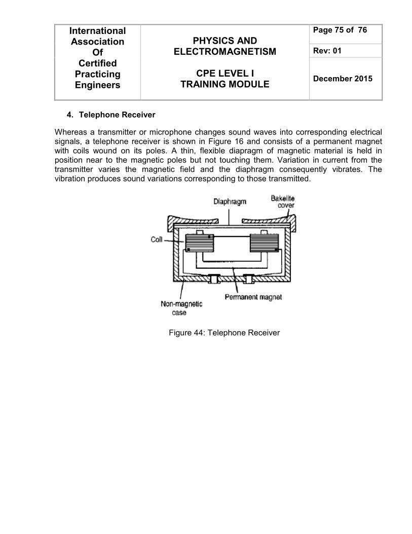
International Association
Of Certified
Practicing Engineers
PHYSICS AND ELECTROMAGNETISM
CPE LEVEL I
TRAINING MODULE
Page 75 of 76
Rev: 01
December 2015
4. Telephone Receiver
Whereas a transmitter or microphone changes sound waves into corresponding electrical signals, a telephone receiver is shown in Figure 16 and consists of a permanent magnet with coils wound on its poles. A thin, flexible diapragm of magnetic material is held in position near to the magnetic poles but not touching them. Variation in current from the transmitter varies the magnetic field and the diaphragm consequently vibrates. The vibration produces sound variations corresponding to those transmitted.
Figure 44: Telephone Receiver
International Association
Of Certified
Practicing Engineers
PHYSICS AND ELECTROMAGNETISM
CPE LEVEL I
TRAINING MODULE
Page 76 of 76
Rev: 01
December 2015
REFERENCES
1. “DOE Fundamentals Handbook Electrical Science Volume 1” by U.S Department of
Energy, Washington DC, 1996.
2. “Electrical and Electronics Principles and technology” by John Bird, Oxford: Newnes,
2003.
3. “Fundamentals of Industrial Electronics” by Bogdan M. Wilamowski, J. David Irwin, Uni
States of America : CRC Press LLC, 2010.
4. “Lessons in Electrical Circuit Volume I – DC” by Tony R. Kuphaldt, 2003.
5. “The Electrical Engineering Handbook” by Wai – Kai Chen, United States of America:
Elsevier Academic Press, 2004.
6. “Newnes Electrical Pocket Book” by E.A. Reeves, Martin J Heathcote, Oxford: George
Newnes Ltd, 2003.
7. “The Electronics Handbook” by John Witaker, US : Taylor & Francis Group, 2005.
8. “The Power Electronics Handbook” by Timothy L. Skvarenina, Unistates of America:
CRC Press LLC, 2002.
9. https://en.wikipedia.org/wiki/Magnet
10. https://en.wikipedia.org/wiki/Electromagnetism
11. http://abyss.uoregon.edu/~js/21st_century_science/lectures/lec04.html
12. http://www.bbc.co.uk/education/guides/zxxbkqt/revision