Embed Size (px)
Citation preview
RETURN ON MARKETING INVESTMENTS IN B2B CUSTOMER RELATIONSHIPS:
A DECISION-MAKING AND OPTIMIZATION APPROACH
Sandra Streukens (Corresponding Author)
Department of Business Studies, Hasselt University
Agoralaan – Building D
BE-3590 Diepenbeek, Belgium
T: +32 11 26 8628
Stan van Hoesel
Department of Quantitative Economics, Maastricht University
PO Box 616, 6200 MD Maastricht, The Netherlands
T: +31 43 3883727 E: [email protected]
First submission at September 1, 2008
Revised submission at March 9, 2009

Sandra Streukens is currently an assistant professor of marketing with the Department of Business
Studies at Hasselt University (Belgium). Her main research interests include services marketing, research
methodology, service employee management, and return on services. Her work is published in
international journals like Marketing Letters, Journal of Economic Psychology, Journal of Business
Research, Industrial Marketing Management, Information and Management, Managing Service Quality,
and International Journal of Service Industry Management.
Stan van Hoesel is professor of operations research with the Department of Quantitative Economics at
Maastricht University (The Netherlands). His main research interests include network design, frequency
assignment, and combinatorial optimization. His work is published in international journals like
Management Science, European Journal of Operations Research, Transportation Science, International
Journal of Production Economics, and Mathematical Programming.
1
ABSTRACT
The basic notion of relationship marketing entails that firms should strive for mutually beneficial
customer relationships. By combine relationship marketing theory and operations research
methods, this paper aims to develop and demonstrate a managerial decision-making model that
business market managers can use to optimize and evaluate marketing investments in both a
customer oriented and economically feasible manner.
The intended contributions of our work are as follows. First, we add to the return on marketing
literature by providing a first decision-making approach that explicitly assesses the optimization
of marketing investments in terms of profitability, effort, and resource allocation. Second, we
show how the risk of marketing investments can be assessed by means of sensitivity analysis.
By means of an empirical study we demonstrate the versatility of our decision-making approach
by assessing various critical decision making issues for business marketing managers in detail.
Furthermore, we show how our decision-making approach can be a valuable extension of
commonly used customer satisfaction studies.
Keywords: Return on Marketing, Relationship Marketing, Optimization, Marketing
Decision Making
2
1. INTRODUCTION
Consistent with the basic tenet of relationship marketing that a company should strive for
mutually beneficial customer relationship (LaPlaca, 2004) there is a strong need for managerial
decision-making models that combine marketing theory with mathematical rigor (Metters &
Marucheck, 2007; Bretthauer, 2004; Boudreau, Hopp, McClain, & Thomas, 2003).
Recent work in business marketing management underscores this premise of uniting soft
customer perceptions and hard objective measures in a single decision-making tool. For instance,
Gök (2008) demonstrates the need for and value of including forward-looking customer
evaluative judgments like satisfaction in marketing performance evaluation. Furthermore,
Seggie, Cavusgil, and Phelan (2007) underscore the need for linking marketing initiatives to
quantifiable financial outcomes. Nevertheless, models that combine marketing theory and
financial performance measures to guide marketing investment decision making are scant in the
literature. Therefore, the aim of our study is to develop and demonstrate a practical and versatile
decision-making approach that assists business market managers in evaluating and optimizing
marketing investments in an economically justified, yet customer-oriented manner.
In line with the aforementioned need for decision-making models that combine marketing
theory with mathematical rigor the two main building blocks of our decision-making model
include relationship marketing theory and operations research techniques. Anchoring the model
in operations research principles permits decision makers to balance marketing revenues and
costs. The use of relationship marketing theory to conceptualize different elements in the
decision-making model allows for customer-oriented decision making. With this study we
contribute to the literature in the following ways. First, compared to existing models (e.g., Rust
et al. 1995; 2004) our approach adds to the return on marketing literature by explicitly
3

optimizing marketing investment profitability both in terms effort level as well as effort
allocation. Second, we show how investment risk can be assessed by examining the robustness of
the model’s projected financial consequences.
The remainder of this paper is structured as follows. Section two focuses on the
theoretical development of our decision-making approach. We start this first section by
providing an overview of our decision-making model. Subsequently, we provide a detailed
explanation of the various elements and links in our decision-making approach. Section three of
this paper summarizes the empirical study conducted to calibrate the customer relationship part,
or more precisely the marketing investment revenues component, of our approach. Building on
the results of this empirical study, the fourth section shows how our model can be used to tackle
critical decision-making issues such as optimizing marketing investment profitability, optimizing
marketing investment effort allocation and assessing marketing investment risk. In the fifth and
sixth section, we respectively discuss the various implications for business market managers and
explain how our optimization approach can be extended to accommodate situations other than
the one illustrated in this paper.
2. MODEL DEVELOPMENT
We start this section with a general overview of the main components of our decision-making
model and their interrelationships. Subsequently, the different components are specified into
detail.
2.1 Overview of the decision-making approach
4
In line with the basis of relationship marketing, the starting point of our decision-making
approach is that customer-firm relationships should be mutually beneficial (see also LaPlaca,
2004). In terms of marketing investments, the idea of mutually beneficial customer-firm
relationships is reflected in the return on marketing approach (see also Rust, Zahorik, &
Keiningham, 1995) proposing that marketing investments should improve a firm’s financial
performance via improvements in customer evaluative judgments. Consequently, an effective
decision-making model guiding marketing investments should thus carefully and explicitly
balance changes in customer’s perceptions stemming from marketing investments and the firm’s
financial consequences of these marketing investments.
To arrive at a decision-making approach to evaluate and optimize marketing investments
that contribute to the establishment of mutual beneficial relationships, the following two
elements are of crucial importance. First, in line with Zhu, Sivakumar and Parasuraman (2004)
our decision-making framework explicitly takes into account both the involved marketing
investment revenues and costs, thereby allowing the firm to conduct an economically justified
analysis of marketing investments. Second, changes in customer evaluative judgments resulting
from marketing investments should be explicitly connected to financial consequences. For this,
we draw upon relationship marketing theory to model the marketing investment revenues in our
approach. Figure 1 below graphically presents the main elements of our decision-making
approach and shows their interrelationships.
--------------------------------------------------------
INSERT FIGURE 1 ABOUT HERE PLEASE
--------------------------------------------------------
The first link (i.e., Link 1) in F
5
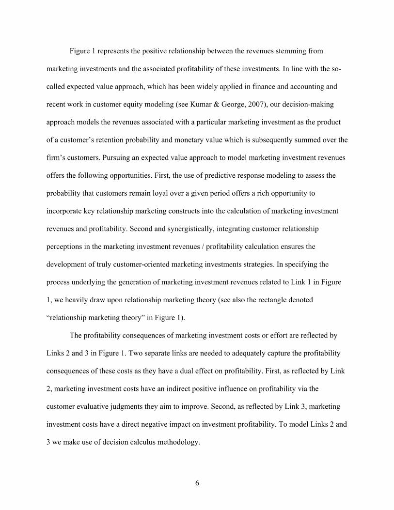
Figure 1 represents the positive relationship between the revenues stemming from
marketing investments and the associated profitability of these investments. In line with the so-
called expected value approach, which has been widely applied in finance and accounting and
recent work in customer equity modeling (see Kumar & George, 2007), our decision-making
approach models the revenues associated with a particular marketing investment as the product
of a customer’s retention probability and monetary value which is subsequently summed over the
firm’s customers. Pursuing an expected value approach to model marketing investment revenues
offers the following opportunities. First, the use of predictive response modeling to assess the
probability that customers remain loyal over a given period offers a rich opportunity to
incorporate key relationship marketing constructs into the calculation of marketing investment
revenues and profitability. Second and synergistically, integrating customer relationship
perceptions in the marketing investment revenues / profitability calculation ensures the
development of truly customer-oriented marketing investments strategies. In specifying the
process underlying the generation of marketing investment revenues related to Link 1 in Figure
1, we heavily draw upon relationship marketing theory (see also the rectangle denoted
“relationship marketing theory” in Figure 1).
The profitability consequences of marketing investment costs or effort are reflected by
Links 2 and 3 in Figure 1. Two separate links are needed to adequately capture the profitability
consequences of these costs as they have a dual effect on profitability. First, as reflected by Link
2, marketing investment costs have an indirect positive influence on profitability via the
customer evaluative judgments they aim to improve. Second, as reflected by Link 3, marketing
investment costs have a direct negative impact on investment profitability. To model Links 2 and
3 we make use of decision calculus methodology.
6
The remainder of this section explains the various elements presented in Figure 1,
captures them in mathematical equations, and brings the elements together in a mathematical
framework that can be used to evaluate and optimize marketing investments.
2.2 Modeling marketing investment revenues
This paragraph focuses on modeling the marketing investment revenues function and the
integration of this function in our decision-making model. First we explain the role of
relationship marketing theory in modeling the marketing investment revenues function. Second,
we show how the resulting revenues function can be incorporated in our mathematical decision-
making model to evaluate and optimize marketing investment decisions.
As outlined above and depicted in Figure 1, the probability that a customer is retained
over a certain time period by the company plays a crucial role in determining marketing
investment revenues (and thus ultimately marketing investment profitability). Consequently,
understanding what drives this customer retention probability is necessary to develop profitable
marketing initiatives. To understand the customer’s retention probability in business settings the
beliefs -> attitude -> behavioral intent model offers a valuable conceptual model (Lewin, 2008;
Lam, Shankar, Erramilli, & Murthy, 2004).
Building on the general structure of the beliefs -> attitude -> behavioral intent model we
used the following constructs in modeling the marketing investment revenues function. In
explaining customer attitudes and behavior, perceived quality and perceived value are considered
the two most important beliefs (Cronin, Brady, & Hult, 2000). Perceived quality is the
consumers’ cognition-based appraisal of an offerings overall excellence or superiority (Zeithaml,
1988). Perceived value captures the customer’s trade-off between sacrifices and returns involved
7
in using a particular market offering (Cronin et al., 2000). Two key attitudinal contructs that play
a role in the formation of customer loyalty are satisfaction and trust (Selnes, 1998; Garbarino &
Johnson, 1999). Satisfaction is the customers’ cumulative evaluation that is based on all
experiences with the company’s offering over time (Anderson, Fornell, & Lehmann, 1994). Trust
is the customer’s confidence that the seller can be relied on to deliver according to their promises
(Nijssen, Singh, Sirdeshmukh, & Holzmueller, 2003). Finally, following common practice in
customer research, we use behavioral intentions as a proxy for customer loyalty. Customer
loyalty is a buyer’s overall attachment to an offering, brand, or organization (Oliver, 1999).
Moreover, similar to other return on marketing models, this study conceptualizes customer
loyalty as the probability of securing the customers’ monetary value over a specific time period
(Rust, Lemon, & Zeithaml, 2004). Table 1 summarizes the key literature regarding the
relationships among the various belief, attitude, and intent constructs defined above.
---------------------------------------------------------
INSERT TABLE 1 ABOUT HERE PLEASE
---------------------------------------------------------
In addition to understanding how customer evaluative judgments relate to marketing
investment revenues, we need to integrate the set of relationships connecting customer beliefs,
attitudes, and behavioral intent into a formal marketing investment decision-making approach.
To achieve this we proceed as follows.
Maintaining with the notion of a chain of effects between beliefs, attitudes, and
behavioral intentions, investments aimed at improving customer quality perceptions (i.e., beliefs)
are assumed to eventually trigger an increase in customer retention probability. Or analogous to
8
Rust et al.’s (2004) return on marketing terminology, customer quality perceptions are retention
probability drivers. Without loss of generality, the remainder of this paper focuses on the
financial consequences of marketing investments aimed at improving customer quality
perceptions. These drivers (i.e, quality perceptions) are denoted as (iy Ii∈ ).
Building on the nomological network connecting quality perceptions to customer
retention, the impact of changes in the various drivers (iy Ii∈ ) due to targeted marketing
investments positively influences customer retention rates and thus eventually marketing
investment revenues. The overall influence of changes in the various drivers on the customer’s
retention probability can be summarized by function . As will be shown in section four of
this paper, function can be determined directly from empirical analysis of the set of
hypothesized relationships among the different customer constructs linking customer quality
perceptions to customer retention.
ci loyyf ,
ci loyyf ,
To ultimately determine the marketing investment revenues, the customer retention
probability is to be multiplied by the amount of customer monetary value that a customer is
likely to generate over a specific time period and summed over all the relevant customers.
Mathematically, this is expressed in Equations (1a) and (1b) below.
( ) ([ ]∑=
−=C
ccccc
CMVloyCMVloyREV1
)0()0( ) (1a)
Where
∑∈
=Ii
iloyyc yfloyci , (1b)
9
In Equation (1a) the term refers to the customer retention probability as a result of some
particular marketing investment, whereas the term is the status quo customer retention
probability and refers to the customer retention probability before the implementation of the
marketing initiative aimed at increasing customer retention. Furthermore, the terms
and refer to the customer monetary value before and after the marketing
investment, respectively. Thus, Equation (1a) implies that marketing investment revenues are the
difference between the current customer revenues (associated with the current level of customer
evaluative judgments) and the revenues that can be expected when marketing investment aimed
at influencing customer evaluative judgments are made. In Equation (1b) the term denotes
the impact of the different drivers on the customer’s probability to remain loyal over some
time period as reflected by the nomological network of relationships connecting quality
perceptions to customer retention probability (see also rectangle named “relationship marketing
theory” in Figure 1).
cloy
cloy )0(
cCMV )0( cCMV
ci loyyf ,
iy
2.3 Modeling marketing investment costs
As reflected by Links 2 and 3 in Figure 1, marketing investment costs or effort have both
a direct negative and an indirect positive effect on marketing investment profitability. The
indirect positive effect stems from the fact that targeted marketing investments (denoted by )
influence customers’ quality perceptions ( ), which through increased loyalty, yield marketing
investment revenues (see also Link 2 in Figure 1). Thus, the quantification of this particular
positive relation between investment effort ( ) and the level of the drivers ( ) is crucial to the
development of our decision making model. We use the response curve proposed in Little’s
ieff
iy
ieff iy
10

(1970) ADBUDG function to estimate this relationship. The value of Little’s (1970) ADBUDG
model is two-fold. First of all, ADBUDG offers a “simple, robust, easy to control, adaptive, as
complete as possible, and easy to communicate with” (Little, 1970 p.466) modeling approach.
Second, as the parameters of the model are calibrated in consultation with managers, the
ADBUDG model reflects Blattberg and Hoch’s (1990) notion that decision quality is best when
both statistical and human input is combined. In general terms, the ADBUDG function is defined
as shown in Equation (2).
i
i
cii
ci
iiii effdeff
abay+
−+= )( (2)
Concerning Equation (2), parameters and restrict driver to a meaningful range
(i.e., ). More specifically, represents the level of driver i (i.e, ) when no marketing
investments are made for this variable (i.e.,
ia ib iy
],[ ii ba ia iy
0=ieff ); corresponds to the value of the driver
when an infinite amount of resources would be invested in this driver (i.e., ).
Parameters and determine the shape of the relationship between and . More
specifically, parameter allows the response curve to be either concave or s-shaped, whereas
parameter reflects the slope of the response curve.
ib
∞→ieff
ic id iy ieff
ic
id
Calibration of the ADBUDG function shown in Equation (2) automatically
provides an estimate of the total level of investment costs, which has a direct negative impact on
the profitability of marketing investments (see also Link 3 in Figure 1). The total level of
marketing investment costs equals the amounts invested in the different specific drivers summed
over all relevant drivers. Thus, as reflects the investment effort needed to influence a ieff
11
particular customer retention driver , the total investment effort associated with a particular
investment strategy aimed at improving a set of drivers can be defined as:
iy
Total efforts ∑∈
−=Ii
ii effeff ))0(( (3)
In Equation (3) the term in the investment level needed to maintain the
level of the drivers (please note that this relationship is implied by Equation (2)). The
levels of the drivers correspond with the parameter in Equation (1a). As indicated
by Link 3 of our conceptual model in Figure 1, the level of total invest effort directly reduces the
profitability of marketing investments.
ieff )0(
iy )0(
iy )0( cloy )0(
2.4 Modeling and optimizing marketing investment profitability
The profitability of marketing investments equals the difference between the revenues
and costs associated with a particular marketing investment. Consequently, the profitability
function, presented in Equation (4), follows directly from the revenue and total investment effort
function expressed in Equations (1a) and (3) respectively.
( ) ( )[ ] [ ]⎥⎦
⎤⎢⎣
⎡−⎥
⎦
⎤⎢⎣
⎡= ∑∑
∈
−
=
−
Iieffeff
cCMVloyCMVloy iicccc
cprofits )0(
1)0()0(
(4)
Similar to the work of Rust et al. (1995, 2004) Equation (4) yields sufficient information
to make marketing investments financially accountable and to compare and evaluate them vis-à-
vis alternative (marketing) investment opportunities. In addition to making marketing
investments financially accountable, optimizing marketing investment profitability is an issue of
great managerial interest (Zeithaml, 2000) which so far has received little attention in the
existing literature.
12
In order to devise marketing investment strategies that maximize profitability, the
expression presented in Equation (4) serves as an objective function in an optimization problem.
The core of this optimization problem is to maximize marketing investment profitability by
finding optimal spending levels for the different drivers . Or equivalently, determining
which spending levels yield optimal levels of customer perceptions regarding the different
drivers as reflected by a maximum level of marketing investment profitability.
ieff iy
ieff
iy
Building on the interrelationships among marketing investment profitability, revenues,
and costs (see also Figure 1), maximizing the profitability function is subject to the following
constraints. The first constraint, presented below in Equation (5a) models the impact of changes
in the input variables on the retention probability as hypothesized by the set of relationships
underlying the loyalty formation process (see also rectangle “Relationship Marketing Theory” in
Figure 1).
iy
∑∈
=Ii
iloyyc yfloyci , (5a)
The second constraint models the effect of investment effort on the level of the input
variables following Little’s (1970) ADBUDG function. As a reminder, this constraint is
modeled as follows (see also Equation (2)).
ieff
iy
i
i
cii
ci
iiii effdeff
abay+
−= )( (5b)
Third, we impose a budget constraint implying that the total investment effort cannot exceed a
pre-set budget B . This budget constraint is summarized in Equation (5c).
∑∈
−Ii
ii effeff ))0(( ≤ B (5c)
13

Finally, we impose a nonnegativity constraint for , which is formally expressed in Equation
(5d).
ieff
0)0( ≥− ii effeff (5d)
Together the objective function and constraints described above yield the optimization
framework presented in Exhibit 1.
Exhibit 1: Overview of the decision-making / optimization framework
[ ( ) ( )[ ] [[ ]
]]
( )
Iiii
Iiii
Iicii
ci
iiii
IiIi
iloyyc
Iiii
C
ccccc
effeff
Beffeffeffd
effabay
yfloyts
effeffCMVloyCMVloy
Ii
i
i
ci
∈
∈
∈
∈∈
∈=
∀≥−
∀≤−
∀+
−+=
∀=
−−−
∑
∑∑∑
∈
0)0(
)0(
)(
..
)0()0()0(max
,
1
In the following two sections we will estimate and calibrate the various parameters
required to implement the decision-making or optimization model. To begin with, section three
describes the empirical study conducted to understand and model the marketing investment
revenues function consisting of the customer’s retention probability and the customer monetary
value (see also Equations (1a) and (1b)). Section four uses the results of the empirical study to
demonstrate the various possibilities our optimization framework in Exhibit 1 offers for
marketing decision making.
14
3. ANALYZING CUSTOMER RETENTION AND CUSTOMER MONETARY VALUE
3.1 Sampling
Survey data needed to estimate the different elements of the marketing investment
revenues function (see also Figure 1 and Equations (1a) and (1b)) were obtained from business
customers of the supplies business unit of a large international operating manufacturer of office
equipment. This business unit sells the supplies (e.g. paper and toner) needed to operate their
office equipment (copiers and printers). Furthermore, the company aims to build long-term
relationship with its customers based on service excellence. The population of this study consists
of B2B customers for which it is economically infeasible to pursue a one-to-one marketing
strategy. Overall, these customers make up approximately 37.6 % of the total customer base.
In total, we obtained an effective response rate of 36.6 % or 183 respondents.
Examination of the sample profile led to the conclusion that our sample is representative of the
underlying target population. Furthermore, all questionnaires were labeled with the customers’
unique ID-code enabling us to link the customer’s perceptual and (objective) sales data.
3.2 Data
All respondents that participated in our study received a questionnaire containing items
on perceived quality, overall satisfaction, perceived value, trust, and behavioral intentions.
Perceived quality was measured by means of 7 attributes that covered the most important product
and service aspects from the customers’ point of view (cf. Rust et al. 1995). Overall cumulative
satisfaction was measured by means of a single item (Anderson et al., 1994). Perceived value (4
15
items) was assessed using a scale that was adapted from the measurement instruments developed
by Dodds, Monroe, and Grewal (1991) and Cronin et al. (2000). Trust (5 items) was measured by
means of the scale developed by Kumar, Scheer and Steenkamp (1995). All above-mentioned
constructs were measured on 11-point Likert scales. The customer’s retention probability was
assessed by measuring the current percentage spent at the company under study relative to the
total amount of money spent at the particular product category (Rust et al., 2004). See Table 2
for an overview of the descriptive statistics of the customer constructs assessed for this study.
Moreover, Table 5 accompanying the application of our decision-making model contains a short
description of each quality item or driver.
Finally, data on customer sales over an 18 month period were obtained from the
company’s data base. To account for customer differences in purchase times, monthly sales were
summed over a three month’s time period.
---------------------------------------------------------
INSERT TABLE 2 ABOUT HERE PLEASE
---------------------------------------------------------
3.3 Estimation procedure customer retention probability
To estimate the relationships explaining the customer’s retention probability, we opted
for PLS path modeling (SmartPLS2.0 M3) as our model contains both formative and reflective
scales.
To restrict the (predicted) retention probabilities to a feasible 0-1 range, all stated
retention probabilities underwent a logit transformation. To our best knowledge no PLS path
modeling software is available to accommodate the resulting non-linear logit curve. To
16
overcome this problem we proceeded as follows. Based on the retention probability we
determined each respondent’s odds ratio. Subsequently, taking the natural logarithm of the odds
ratio and specifying it as a formative indicator for the loyalty construct allowed us to estimate it
as linear function of its hypothesized antecedents.
To evaluate the statistical significance of the various parameter estimates we construct
bias-corrected bootstrap percentile confidence intervals based on 5,000 bootstrap samples.
3.4 Estimation procedure customer monetary value
In line with Venkatesan and Kumar (2004) customer monetary value ( ) is modeled
as a function of past behavior and customer characteristics such as customer size, customer type,
and relationship length. The following issues warrant specific attention when analyzing panel
data. First, to accommodate the problem of endogeneity due to the use of lagged dependent
variables which are needed to examine the effect of past behavior, we used the first difference
specification of customer monetary value (
cCMV
1,., −−=Δ tctctc CMVCMVCMV ) as the dependent
variable in our model and as an independent variable (Baltagi 2008, p.148). Second, to
examine whether a one-way or two-way error component random effects
2, −tcCMV
1 model is most
appropriate a series of Breusch-Pagan need to be conducted (Wooldridge, 2002). The dynamic
regression model for the situation at hand is summarized in Equation (6)
ticcc
cctctctc
RELTYPTYPSIZESIZEQUANCMVCMV
,765
431,22,1,
2121
εγγγγγγγ
++++++++=Δ −−
(6)
1 A fixed effects panel data model was not feasible as all regressors except the lagged dependent variable are time constant.
17
Where refers to the quantity purchased in US dollars by the customer in period1, −tcQUAN 1−t ,
and are dummies reflecting the size of the customer expressed in past sales
volume (entire population is split into four groups based on quartiles, only the lowest three
quartiles were included in our sampling frame), and are dummies reflecting the
product line(s) the customer uses. All four dummy variables can be considered time-invariant.
The variable denotes the length of customer’s relationship with company measured in days
since the first purchase. The variables
cSIZE1 cSIZE2
cTYPE1 cTYPE2
cREL
tcCMV ,Δ and are as defined above. To estimate
the dynamic regression model expressed in Equation (6) we used SAS v9.2’s PROC PANEL.
2, −tcCMV
3.5 Empirical results customer retention probability
We begin with evaluating the psychometric properties of the various scales used to tap
customer evaluative judgments. In assessing the performance of the scales used in this study it is
important to distinguish between (multiple-item) reflective and formative scales (MacKenzie,
Podsakoff, & Jarvis, 2005). In this study, perceived value and trust are considered reflective
scales, whereas perceived quality is considered a formative scale.
Concerning the reflective scales, unidimensionality is evidenced by the fact that the first
eigenvalue matrix of the respective item correlation matrices exceeds one, whereas the other
eigenvalues are less than one (Tenenhaus, Esposito Vinzi, Chatelin, & Lauro, 2005).
Furthermore, reliability was evidenced as for both reflective scales the internal consistency
statistic passed the 0.70 cut-off value. Support for the reflective scales’ within-method
convergent validity is provided by the high average variance extracted levels and the magnitude
and significance of the indicator loadings.
18
Regarding formative scales the most relevant type of validity is content validity
(Diamantopoulos & Winklhofer, 1999). The fact that we designed the scale assessing perceived
quality scale to encompass all relevant business processes together with the significant loadings
provides substantial evidence for the content validity of this formative scale.
Finally, for all scales used in this study discriminant validity was evidenced as all
between-construct correlation coefficients significantly differ from an absolute value of 1. See
Table 2 for the relevant figures regarding the evaluation of the scales’ psychometric properties.
Turning to the empirical results for the hypothesized structural relationships underlying
the revenue generating process, which are presented below in Table 3, the bootstrapped
2R confidence intervals indicate that the theoretical model has a good fit to the data.
Furthermore, as indicated by the statistical significance for the majority of the regression
coefficients it can be concluded that also in B2B settings managing customer attitudes and
perceptions is vital in creating customer loyalty. Thus, as evidenced by the chain of effects
connecting customer beliefs and attitudes to customer behavior, directing investment effort at
improving customer beliefs such as perceived quality offers an important opportunity to make
customers more loyal. Put differently, marketing investments aimed at improving customer
evaluative judgments are an effective way to enhance revenues.
---------------------------------------------------------
INSERT TABLE 3 ABOUT HERE PLEASE
---------------------------------------------------------
Despite the insights to manage customer loyalty among business customers, these
empirical results alone are insufficient to resolve important management issues such as the
optimal amount and optimal allocation of investment efforts needed to improve customer
19

evaluative judgments in an economically justified way. This underscores the need for a formal
decision-making approach to evaluate and manage marketing investments even further.
3.6 Empirical results customer monetary value
Comparing the results for the Breusch-Pagan test for both a one-way and two-way error
component random effects model showed that a one-way error component random effects model
is appropriate for the situation at hand ( ). Furthermore, as evidenced by the 00.1)1(2 =Δχ
2R value of 0.54 our model shows a good fit to the data. The estimation results for the various
parameters in our dynamic regression model are presented below in Table 4.
---------------------------------------------------------
INSERT TABLE 4 ABOUT HERE PLEASE
---------------------------------------------------------
The results in Table 4 demonstrate that past customer monetary value, past purchase quantity,
and customer size are important indicators of future customer monetary value.
Building on the empirical results providing insight into the customer loyalty formation
process and customer monetary value (i.e. key elements of the marketing investment revenues
component of our model), section four focuses on how these empirical results can be used to put
our marketing investment decision-making approach into practice.
4. APPLICATION OF THE DECISION-MAKING APPROACH
This section demonstrates how our decision-making approach presented in Exhibit 1 can
assist business market managers in tackling the following vital marketing investment issues:
what is the optimal level of marketing investment effort to maximize profitability, what is the
20

projected return on investment for a specific investment initiative, how should we optimally
allocate the investment efforts over the drivers, and how risky is the projected investment
strategy.
Before we can assess these issues, we first need to calibrate the functions pertaining to
marketing investment revenues (i.e. Link 1 in Figure 1) as well as the indirect positive and direct
negative effect of investment effort on investment profitability (i.e. respectively Links 2 and 3 in
Figure 1). Please note that additional detailed background information on the calibration of the
model components can be found in the appendices to this paper.
4.1 Calibrating the investment revenues function
The impact of each driver on the customer’s retention probability, and thus ultimately
marketing investment revenues and profitability, as reflected by , can be calculated directly
from the empirical data presented in Tables 2 and 3 as follows. Given that the model describing
the revenue generating process is non-recursive (acyclic), the total influence of each input
variable on is summarized below in Equation (7) and will be referred to as
iy
ci loyyf ,
iy cloycloyy ,1
λ in the
remainder of this paper.
∑ ∏→ ∈
⎟⎟⎠
⎞⎜⎜⎝
⎛==
)(: ),(,,
ci ci
ciciloyyP Ployy
ijloyyloyy wf λ (7)
In Equation (7) are the different marginal effects of the relevant independent variables on the
relevant dependent variables as hypothesized in our relationship marketing theory model (see
also Figure 1). In words, Equation (7) states that the effect of a unit change in driver on the
customer’s retention probability can be computed by calculating the product of the
ijw
iy
cloy
21

coefficients belonging to each of the separate relationships connecting and , and
subsequently summing these products over all relevant paths connecting and .
ijw iy cloy
iy cloy
It is important to note that the computation of the marginal effects depends on the
functional form of the equations describing the various links in the structural model
connecting and . For relationships characterized by a linear functional form equals the
relevant unstandardized regression coefficient. For the logit equation with as dependent
variable, is computed as
ijw
iy cloy ijw
cloy
ijw2)...(
)...(
)1( 2211
2211
kkjjj
kkjjj
xwxwxwa
xwxwxwa
ij eew +++++−
++++−
+∗ where the -parameters are the
relevant unstandardized coefficients belonging to the independent variables. All needed
unstandardized regression coefficients result from our empirical study (see also Tables 2 and 3).
Following the idea expressed in Equation (7), Table 5 summarizes the average influence of a
one-unit change in on a customer retention probability for the situation at hand.
ijw
k
iy cloy
The dynamic regression results presented in Table 4 are used to predict the customer
monetary value over the next time period (quarter). Together the customer retention probability
as a function of drivers and the estimates for each customer’s monetary value provide the
necessary information to model the customer revenues function reflected by Equation (1a).
iy
4.2 Calibrating the investment effort functions
To capture the profitability consequences of the marketing investment costs the
ADBUDG based function expressed by Equation (2) needs to be calibrated. It should be noted
that once we calibrated this function for each of the drivers (i.e., quality elements) we
automatically have an estimate for the total investment effort as reflected by Equation (3). To
22

calibrate the function between investment effort ( ) and drivers ( ) as captured by Equation
(2), we first need to understand what actions are capable of influencing the customer’s
perceptions regarding these drivers. Interviews with the company’s customer service managers
and several customers yielded insight in this matter. Second, we need to assess how various
levels of these actions, reflecting different investment effort levels, relate to changes in the
customer’s perceptions of the various drivers (i.e., rating shifts). As shown in Appendix 1 a set of
standard questions is asked to determine the shape of the function (i.e., ADBUDG parameters
and ) between investment effort and the driver perceptions (see also the original work of
Little (1970) or the more recent application of Dong, Swain, and Berger (2007)).
ieff iy
ic id
For reasons of confidentiality we use an example cost-function in the current application
of our decision-making model. As each practical application of our model is likely to have a
unique cost-function reflecting the idiosyncrasies of each setting, the use of an example cost-
function does not limit the applicability of our model. Regarding the current application,
parameter was set to 1, thereby reflecting that the investments aimed improving customers’
quality perceptions are subject to diminishing returns (Little, 1970). For parameter a value of
$50,000 was chosen to approximate the underlying cost function. Finally, as the purpose of
parameters and is to restrict changes in to a meaningful range, these parameters are
implicitly determined by the endpoints of the scales we used to measure the customer’s
perceptions concerning the various drivers. Consequently, parameter is set to 1 (the lowest
value of the measurement scale used) and parameter is set to 11 (the highest value of the
measurement scale used).
ic
id
ia ib iy
ia
ib
23

4.3 Investment strategy
Rust, Moorman, and Dickson (2002) conclude that financial returns on marketing
investments can arise from increasing revenue by increasing satisfaction, decreasing costs, or
both. Furthermore, investment profitability may vary as a function of retaining current customers
and/or gaining new customers (Rust et al. 2004). Although many investment strategies are
possible and no company can afford to ignore both customer acquisition and cost reduction in
favor of respectively customer retention and revenues, the current application demonstrates the
optimization of marketing investment profitability as a result of increasing in revenues due to
enhanced customer retention. This choice is based on Rust et al. (2002) who show that revenues
expansion due to increased satisfaction yields superior results over cost reduction strategies.
Furthermore, the work of Fornell and Wernerfelt (1987, 1988) evidences that customer retention
is an economically more feasible strategy than customer acquisition. Despite the focus on
revenues expansion through customer retention, section six of this paper later elaborates how our
optimization framework can be adapted to accommodate other situations such as designing
optimal investment strategies for both customer retention and acquisition.
Below we outline the results regarding the application of our decision-making model.
The software package AIMMS2 was used to perform all optimization analyses. More specifically
we opted for a subgradient optimization method. Furthermore, in demonstrating the applicability
of our optimization framework two alternative situations are presented. First, no limit is assumed
on available investment resources, that is, the budget restriction is relaxed. Second, we will
demonstrate the use of our decision-making approach in situations where there is a budget
2 AIMMS stands for Advanced Interactive Mathematical Modeling Software for more information see also www.aimms.com and Appendix 1 to this paper.
24

constraint. Overall, the use of our decision-making framework will proceed in exact the same
manner regardless of whether a budget constraint is imposed or not.
4.4 Optimal level of investment effort
Coherent with Rust et al.’s (1995) idea that marketing investments should be optimized
rather than maximized, the concave relationship between investment effort and investment
profitability for the current application presented in Figure 2 further underscores the need to
carefully balance costs and revenues when evaluating marketing investments. Put differently,
Figure 2 illustrates that it is possible to over-invest in marketing initiatives in terms of
profitability and that an optimum investment level yielding a maximum investment profitability
exists.
---------------------------------------------------------
INSERT FIGURE 2 ABOUT HERE PLEASE
---------------------------------------------------------
Our decision model can be used as follows to determine this optimum investment level.
Analytically, the optimum investment level follows from the derivative of our profit function. In
general, marketing investments remain economically feasible as long as the derivative of the
profit function is larger or equal to zero. The optimal level of investment level is reached when
this derivative equals zero. Setting the derivative of the profit function equal to zero and solving
this equation for the situation at hand, shows that an optimal investment level of $42,000 yields a
maximum investment profitability level of $8,894.
It should be stressed that our decision-making model is not restricted to finding a
maximum level of marketing investment profitability in situations were the amount of available
25

investment resources is unlimited (i.e. no budget restriction applies). To further illustrate the
versatility of our decision-making model we subsequently assume that a business market
manager has a limited budget of $10,000 available for making marketing investments. Our
approach also is suitable for addressing the issue of how to get the most out of this restricted
amount of resources. Running our optimization model with the budget constraint set to $ 10,000
points out that this budget can lead to a maximum marketing investment profitability level of
$4,480.
As our decision-making approach clearly and directly provides estimates of the level of
investment effort needed to realize a certain level of profitability, the rate of return of
investment3 ( ) can be computed as shown in Equation (8). ROI
%100*.
.⎟⎟⎠
⎞⎜⎜⎝
⎛ −=
efforttotefforttotprofitsROI
(8)
Using Equation (8) shows that the rates of return on investment are 21.18% and 44.80% for the
situation without (i.e., investment level of $42,000) and with (i.e., investment level of $10,000) a
budget constraint respectively.
In addition to determining the optimal level of investment effort, an optimal allocation of
this investment effort is equally important in maximizing investment profitability (Mantrala,
Sinha, and Zoltners, 1992).
4.5 Optimal allocation of investment effort
3 Please note that the formula to assess the rate of return on investment does not exclude the use of more advanced calculations such as including the discounted residual value or using the discounted value of the cash flow in determining the rate of return. We would like to thank one of the reviewers for bringing this to our attention.
26

In determining the optimal allocation of the investment budget over the various drivers,
the (derivative of the) profit function plays again a crucial role. In particular, the optimal
allocation of investment effort over the different drivers is determined by
the absolute and relative magnitude of the partial derivatives of the profit function with respect to
various effort levels needed to improve the different drivers.
∑∈
−Ii
ii effeff ))0(( iy
ieff
In general terms our model determines the optimal allocation of the available investment
budget effort as follows. Any optimal allocation starts with assigning all available investment
effort to the driver for which the partial derivative of the profit function with respect to
investment effort is highest, say driverieff p . Eventually each partial derivative decreases,
reflecting diminishing returns on investment. As such, the partial derivative with respect to at
some stage will equal the partial derivative with respect to . Here driver is the driver for
which the partial derivative of the profit function with respect to effort is overall second highest.
Upon reaching this equilibrium of partial derivatives, the optimal allocation is maintained by
dividing the remaining available investment effort over both drivers and in such proportions
that the partial derivatives of the drivers remain equal. This proportion depends on the ADBUDG
parameters , , , and , and the impact of each driver on investment profitability,
peff
qeff q
p q
ia ib ic idci loyy ,λ .
This process of comparing the profit function’s partial derivatives belonging to the different
drivers continues until the entire budget is spent.
For the situation at hand we now demonstrate how the optimal investment level
determined previously needs to be allocated to indeed achieve the maximum level of investment
profitability. To do this we again run the optimization framework presented in Exhibit 1, setting
the budget constraint equal to $42,000 (i.e., optimal investment effort level). The results of this
27

analysis are presented in Table 5. Likewise, we determined the optimal allocation of resources
for the situation in which there is only a limited budget of $10,000 available for marketing
investments (see also Table 5).
-------------------------------------------------------
INSERT TABLE 5 ABOUT HERE PLEASE
-------------------------------------------------------
The model results on the optimal allocation of investment efforts presented in Table 5
reveal the following. In the situation in which we have an boundless investment budget to obtain
the overall marketing investment profitability maximum (i.e., an investment budget of $42,000),
the maximum investment profitability level of $8,894 is obtained if 16.94% of the budget (or
$7.114) is allocated to improving customer perceptions regarding the driver “delivery” and
83.06% of the budget (or $34.886) is allocated to improving customer perceptions regarding
driver “product related quality”. Turning to the situation in which a limited investment
budget of $10,000 is assumed, our model indicates that the maximum possible level of marketing
investment profitability of $4,480 is obtained when the entire budget is directed at improving the
driver “product related quality”. These allocation schemes are optimal in the sense that all
investment effort allocation schemes different from the derived optimal allocation scheme yield
investment profitability levels lower than the projected maximum levels of $8,894 (effort level of
$42,000) and $4,480 (effort level of $10,000) respectively.
4y
5y
5y
Finally, to translate the various optimally allocated investment amounts aimed at
improving the different drivers, the input data used to calibrate the relationship between
customer driver perceptions and investment costs (see also ADBUDG function in Equation (2))
should be used for interpolation. For example, the $7,114 suggested to improve driver 4y
28

“delivery” could correspond with closing contracts with a logistics services company to ensure
emergency on-time delivery when needed.
4.6 Investment risk: assessing the robustness of the solution
All (marketing) investments entail uncertainty as the actual financial returns may differ
from what was predicted or expected. Consequently, thorough decision making regarding
(marketing) investments requires evaluating the projected returns in light of this uncertainty or
risk. As risk is reflected by the variability of financial returns (Brealey & Myers, 2000),
examining the robustness of the projected profitability as a function of changes in the
optimization framework’s parameters provides an excellent way to assess the level of risk
associated with the marketing investment decision at hand. Comparable to the notion of risk as
variability in returns, the robustness of the solution refers to the variation in the projected optimal
financial returns and the financial returns that can be expected under a different set of parameters
in the optimization framework. One particular operations research techniques that is valuable in
assessing the variability or robustness of the financial returns predicted by our optimization
framework is nominal range sensitivity analysis (Morgan & Henrion, 1990; von Winterfeldt &
Edwards, 1986). Below we introduce this technique and demonstrate how it can be applied to
assess the robustness or risk of the projected investment schemes.
Nominal range sensitivity analysis evaluates the effects on a model’s output due to
changes exerted by varying individual model parameters across a range of plausible values while
keeping the other parameter values at the nominal or base-case values. The robustness of the
model is subsequently expressed as the positive or negative percentage change compared to the
nominal solution (Frey & Patil, 2002). For the situation at hand, nominal range sensitivity
29

analysis is used to assess how the projected optimal solution differs as a function of changes in
the parameters of the model explaining the relationship dynamics4.
Regarding the set of structural relationships connecting the input variables to , the
impact of a change in one of the structural model’s relationships can be determined as follows. If
the weight of a certain relation is changed, say from to
iy cloy
),( lk klw δ+= klkl ww' , and all other
relations remain unchanged, i.e., parameter )),(),((' lkjiww ijij ≠= qp ,λ describing the influence
of driver on outcome variable as expressed by Equation (7) changes to as expressed by
Equation (9). Please see Appendix 1 for the complete derivation of Equation (9).
pz qz ',qpλ
δλλλλ qlkpqpqp ,,,'
, += (9)
Using Equation (9) we determine the projected investment profitability for various level
of δ and compare these figures to the initial optimal investment profitability. In calculating the
projected profitability level as a function ofδ , we use the investment level and investment
allocation scheme that were considered optimal when initially solving the optimization model.
Table 6 below summarizes the results for the nominal range sensitivity analysis for the situation
at hand.
-------------------------------------------------------
INSERT TABLE 6 ABOUT HERE PLEASE
-------------------------------------------------------
Based on the outcomes of the sensitivity analysis, business market managers can see how
much the projected marketing investment profitability deviates from the original optimal
profitability level as a function of changes in the decision-making model’s parameters. Together
4 For assessing the robustness of the solution due to changes in the cost function or the dynamic regression equation used to model the customer monetary value a similar procedure can be followed.
30
with the expected return on investment of the original optimal solution, the outcomes of the
sensitivity analysis provide the required information to make a risk-return trade-off for particular
marketing investment initiatives.
5. DISCUSSION AND IMPLICATIONS
Building on relationship marketing theory and operations research techniques, the aim of
this study was to develop a decision-making approach that enables business market managers to
effectively manage customer relationships in both a customer-oriented and economically
justified manner. Regarding the intended contribution of our work the following elements can be
discerned. First, we developed and demonstrated a general applicable decision-making or
optimization framework to assess critical management issues related to evaluating and
optimizing marketing investments. Second, we introduced the concept of sensitivity analysis to
assess and understand marketing investment risk.
In line with these two contributions, it needs to be emphasized that although the
optimization of marketing efforts to strengthen customer-firm relationship is an often-stated
management goal, little work exists on how this can be actually achieved in both a customer-
oriented and economically sound manner. This is especially relevant as maximizing financial
performance involves optimizing customer perceptions rather than maximizing them. Therefore,
the development of our decision-making approach is a logical evolutionary next step in the area
of return on marketing initiated by the seminal work of Rust et al. (1995).
In terms of managerial implications we believe our decision-making framework
positively impacts business marketing practice is the following ways. First, our optimization
framework provides a clear-cut answer to the key issues of how much to invest and how to
31

allocate these resources in order to maximize marketing investment profitability. Moreover, as a
consequence of explicitly balancing the cost and benefits of marketing investments the
accompanying rate of return on investment can be readily computed. Besides the informative
value of the return on investment figure in isolation, the rate of return stemming from our
optimization framework can be compared with alternative and competing investment
opportunities such as the purchase of a new piece of equipment. Second, we show how
sensitivity analysis of the optimal solution provides a proxy for risk. Consequently, our approach
enables decision makers to form a well-informed risk-return trade-off when evaluating different
and possibly competing investment opportunities to get the most of their scarce resources. Third,
in terms of implementing our decision-making framework in practice it should be stressed that
the input needed to calibrate the various elements of the framework are in close reach of the
company. Data on customer perceptions needed to model the investment revenues are often
already collected by companies on a regular basis, whereas data on customer monetary value is
typically readily available in the companies’ internal records. Furthermore, the calibration of the
ADBUDG function to link investment efforts to marketing investment drivers follows well
established lines and requires a relatively limited amount of qualitative research. Fourth, our
decision making approach can be used to evaluate and compare different (marketing)
investments. Although the main focus of the current paper was on optimizing investment effort
and allocation to maximize profitability without imposing a budget constraint the application of
the framework is not limited to this. The optimization analysis can be conducted regardless of the
available level of investment effort (i.e., investment budget) by imposing a budget constraint.
Furthermore, besides searching for an optimal solution the framework can also be used to
evaluate and compare the financial consequences of different (marketing) investment initiatives.
32
Fifth, even though the (financial) data used to calibrate the optimization framework is specific
for each company, the structure of the model and its various elements are generally applicable.
As will be shown in section six, the general structure of our decision making approach can be
easily adapted to different situations than demonstrated here.
6. LIMITATIONS AND EXTENTIONS OF THE OPTIMIZATION FRAMEWORK
Part of the strength of a research project lies in the recognition of its limitations. Although
the principal purpose of our empirical study (see also section three) is to serve as a means to
demonstrate our decision-making approach, it is relevant to acknowledge that the current sample
is not strong enough to draw conclusions on the customer-firm relationship dynamics in business
markets in general. More specifically, the fact that data were used from a single company
together with the relatively small sample size and its narrow focus seriously limit the
generalizability of our empirical findings regarding customer relationship management theory in
business settings. Other limitations also include the restricted focus on customer retention for a
single company/brand, the exclusion of possible customer differences regarding the various
elements of our optimization framework, and the unavailability of data to model longitudinal
effects. Furthermore, we did not account for the possible impact of switching costs in explaining
customer loyalty intentions. Although probably of minor concern in the current setting, switching
costs may be an important determinant of loyalty intentions as evidenced by the work of Han and
Sung (2008).
Despite these limitations it might be interesting to show how our optimization model can be
extended to incorporate these issues. First, building on the work of Blattberg, Getz, and Thomas
(2001) the revenue function in our framework can be extended to include the effects of new
33
customer acquisition. Furthermore, similar to the work of Rust et al. (2004) brand switching
effects can be incorporated in our optimization framework by using a switching matrix rather
than the customer’s retention probability. Likewise, the model used to explain customer loyalty
may be extended to include elements such as perceived switching costs. Second, customer
heterogeneity may be explicitly modeled by using specific analysis techniques such as random
effects models or MCMC models to estimate the revenue part and subsequently integrate these
equations in the optimization model. Third and final, marketing investment efforts may differ in
their degree of persistence in influencing marketing investment drivers. On one hand we have
investments, such as a computer for better information processing that once it is done, its effect
on customer evaluative judgments persists during the succeeding periods. On the other hand, we
have marketing initiatives such as investments in staff for which the effects on customer
evaluative judgments are reduced once the staff is replaced. To account for these temporal
effects the ADBUDG function can be extended with a persistence factor κ, which is high for
investments that have a long lasting effect, and low for investments that have a short-term effect
only, whereas time series or panel data techniques can be employed to capture dynamic effects in
shaping customer evaluative judgments.
7. CONCLUSION
The aim of relationship marketing is to build customer-firm relationships that benefit both
parties. In order to achieve this, there is a great need for management tools that quantify both the
positive and negative consequences of marketing investments directed at building mutually
beneficial customer-firm relationships. The decision-making framework put forward in this
paper offers business market managers with a tool to manage marketing investments in both an
34

economically justified and customer oriented manner. As one of the few existing studies that
combines operations research techniques with relationship marketing knowledge in designing a
marketing investment decision-making approach, we believe that our work contributes to both
business marketing practice and research. In particular our paper extensively shows how our
decision-making approach can be used to assess key marketing investment decision issues such
as the amount of effort needed to optimize profitability, the calculation of the rate of return on
investment, and the design of an optimal investment resource allocation scheme.
35
APPENDIX 1
Appendix 1 contains additional computational details concerning the application of our decision-making
model.
1. MODELING THE MARKETING INVESTMENT REVENUES FUNCTION
The two main elements in our marketing revenues function are customer ’s probability to remain
loyal over a time period and his monetary value over that period. Below we outline how we estimated
both elements of the revenue function.
c
1.1 Probability to remain loyal
To include a set of non-recursive structural relationships describing a particular behavioral process in
a mathematical decision-making or optimization model the following procedure needs to be followed.
First, estimate a structural model describing the relevant relationships among key constructs using SEM
or regression-based techniques. Second, use network analysis to determine the total influence of some
input variable or driver on a particular outcome variable . Here, the following principles apply. For
a non-recursive (acyclic) model in which the variables are indexed in a way that all relations are of the
type , i.e., only lower indexed variables influence higher indexed variables (Ahuja,
Magnanti, and Orlin, 1993), the influence of any variable on any other variable can be expressed as
presented below in Equation (A1.1). If we denote the change in each variable by , then
pz qz
)(),( jizz ji <
)( jizi < izΔ
∑∈<
Δ=ΔAjiji
iijj zwz),(:
(A1.1)
For computing the total influence of driver on outcome variable consider all paths connecting
to , and determine the sum of the lengths of these paths. The length of each path is given by the
product of the weights of the separate arcs of the path. In mathematical terms, the calculation of the total
influence of on , denoted by
pz qz pz
qz
pz qz qp ,λ , is expressed below in Equation (A1.2).
∑ ∏→ ∈
⎟⎟⎠
⎞⎜⎜⎝
⎛=
)(: ),(,
qp jizzP Pzzijqp wλ
(A1.2)
In Equations (A1.1)-(A1.2) are the different marginal effects of the relevant independent variables on
the relevant dependent variables in the set of structural relationships. Please note that the computation of
the relevant marginal effects depends on the functional form of the equation. For the situation at hand, the
ijw
36

parameter pqλ needs to be determined for each individual respondent as a consequence of the non-
constant marginal effects for logit functions.
1.2 Customer monetary value
Data on customer monetary value typically have a panel design, implying that data is collected
across individuals over time. To estimate these models that data set needs to be constructed as having
rows where denotes the number of respondents and T are the various time periods over which we
collected information about the respondents. To model the data at hand we opted for a dynamic panel data
model. Dynamic panel data models are characterized by the presence of a lagged dependent variable
among the regressors and are generally expressed as:
NT N
TtNcuxyy ctcttcct ,...,1;,...,1'1, ==++= − βδ ; (A1.3)
Where denotes the score on variablecty y of respondent at time t , are the scores of the
respondent on
c ctx
thc − K regressors at time t , δ and β are regression coefficients, and is the model’s
error component. In modeling panel data the following aspects need to be considered carefully.
ctu
First of all, due to the inclusion of a lagged-dependent variable as independent variable the assumption of
exogeneity no longer may hold. To alleviate the effects of endogeneity Baltagi (2008, p.148) advises to
replace the dependent variable by its first difference specification cty 1, −−=Δ tcctct yyy and to use
as an instrument for the lagged dependent variable regressor. Second, in contrast to regular cross-
sectional regression models, the disturbance term in panel data regression models may consists of
following elements: a time-invariant unobservable individual specific effect
2, −tcy
ctu
cμ , an individual-invariant
time effect tλ , and random remainder error ctυ . Depending on whether tλ is equal to zero or not, a one-
way error component model ( ctcctu υμ += ) or a two-way error component model ( cttcctu υλμ ++= )
applies respectively. A Breusch-Pagan Lagrange multiplier test formally assesses whether the hypothesis
of tλ being equal to zero is rejected or not. Finally, the parameter reflecting the time-invariant individual
specific effect, cμ , can be either modeled as a fixed or random effect. A Hausman specification test can
be performed to assess whether a fixed or random effects model specification is preferred.
2 MODELING THE MARKETING INVESTMENT COST FUNCTION
The relationship between investment effort and the level of the drivers is modeled using the
ADBUDG model suggested by Little (1970). This model offers a simple and flexible tool to calibrate a
37

variety of S-shaped or concave response functions. The general form of the ADBUDG-function
describing the relationship between effort ( ) and response is defined as follows: ieff iy
i
i
cii
ci
iiii effdeff
abay+
−+= )( (A1.4)
Where: iy = Perceptual variable at which effort is directed / driver
ieff = Investment effort in $
ia = Minimum value of when iy 0=ieff
ib = Upper asymptote of scale assessing (corresponds with iy ∞→ieff )
ic = Parameter determining shape of response function. Function is concave when and S-
shaped when
10 << ic1>ic
id = Parameter determining shape of response function
Given that the model has only four parameters, only four data points are necessary to calibrate the
function in Equation (A1.4). Those four parameters are determined based on interviews with the decision-
makers and/or the people at whom the efforts are directed (e.g., customers). Typically, these interviews
focus on the following four questions:
1) Regarding i what is the current level of effort ( ) and to what evaluation does that lead ( )? The
pair of point corresponds to on the ADBUDG response curve.
ieff iy
))0(,)0(( ii yeff
2) If effort is reduced to 0 what will then be the evaluation regarding ? This provides the value
for parameter . Usually, reflects the lowest value of the scale on which the perceptions are
measured.
ieff iy
ia ia
3) If effort approaches infinity when will than be the value of ? This answer provides the value
for parameter . Usually, reflects the highest value of the scale on which the perceptions are
measured.
ieff iy
ib ib
4) If compared to the current situation effort is doubled to what level of would that lead? ieff )0( iy
3 THE DERIVATIVE OF THE PROFIT FUNCTION
The derivative of the profit function plays a pivotal role in optimizing marketing investment
profitability in terms of optimal investment effort level and the optimal allocation of investment effort.
Without engaging in the complex and tedious process of specifying the exact specification of the
derivative of the profit function, the following paragraph provides sufficient information to obtain an
38

intuitive feel for the role the derivative of the profit function plays in the optimization analysis. Please
note that we disregard below the investments needed to main the status quo for the sake of simplicity.
The marketing investment profit function is a composite function of the marketing investment
revenue function and the marketing investment cost function. As can be clearly seen in Exhibit 1, the
dependent variable in the marketing investment revenues equation is a function of the different
drivers , which in turn are a function of marketing investment effort as implied by the ADBUDG-
model. Thus, is both a function of intermediate variables and independent variable . According
to the chain rule, the derivative of the marketing investment profit function with respect to is in the
format of
cloy
iy ieff
cloy iy ieff
ieff
1−∂∂
⋅∂
∂=
∂∂
i
i
ii effy
yprofit
effprofit
. That is, the derivative of the profit function with respect to is
a function of the derivative of the profit function with respect to and the derivative of with respect
to . The term arises from the fact that the total invest effort function is a constant term.
ieff
iy iy
ieff 1−
The derivative of the profit function with respect to depends on the magnitude and functional form of
the relationships connecting and (proof of the diffentiability of the revenue function can be
obtained from the authors upon request). The derivative of with respect to equals
implying that this derivative depends on all ADBUDG-
parameters.
iy
cloy iy
iy ieff
( ) 2111−−− +− ii c
iic
iiiic
iiii effdeffadceffbdc ( )
As long as 0≥∂∂
ieffprofit
investments remain feasible as the incremental investment revenues outweigh the
incremental investment efforts.
4 SENSITIVITY ANALYSIS
Mathematically, the notion of nominal range sensitivity analysis is as follows. If the weight of a
certain relation is changed, say from to ),( lk klw δ+= klkl ww' , and all other relations remain
unchanged, i.e., parameter )),(),((' lkjiww ijij ≠= qp ,λ describing the influence of driver on
outcome variable as expressed by Equation (A1.2) changes to as follows.
pz
qz ',qpλ
39

∑ ∑ ∏∏∑ ∏
∑ ∏∑ ∏
∑ ∏∑ ∏
∑ ∏
∈→ ∈→ −∈∈∉→ ∈
∈→ −∈∉→ ∈
∈→ ∈∉→ ∈
→ ∈
⎟⎟⎠
⎞⎜⎜⎝
⎛+⎟⎟⎠
⎞⎜⎜⎝
⎛+⎟
⎟⎠
⎞⎜⎜⎝
⎛=
+⎟⎟⎠
⎞⎜⎜⎝
⎛+⎟
⎟⎠
⎞⎜⎜⎝
⎛=
⎟⎟⎠
⎞⎜⎜⎝
⎛+⎟
⎟⎠
⎞⎜⎜⎝
⎛=
⎟⎟⎠
⎞⎜⎜⎝
⎛=
PlkzzP PlkzzP lkPzzij
Pzzij
PlkzzP Pzzij
PlkzzPkl
lkPzzij
PlkzzP Pzzij
PlkzzP Pzzij
PlkzzP Pzzij
zzP Pzzijqp
qp qp jijiqp ji
qp jiqp ji
qp jiqp ji
qp ji
www
www
ww
w
),(:)(: ),(:)(: ),(),(),(),(:)(: ),(
),(:)(: ),(),(),(:)(: ),(
),(:)(: ),(
'
),(:)(: ),(
'
)(: ),(
'',
)(
δ
δ
λ
(A1.5)
The first two terms in the last row of Equation (A1.5) add up to , whereas the last term (excluding
parameter
qp,λ
δ ) in the last row of Equation (A1.5) can be written as:
qlkpzzP Pzz
ijzzP Pzz
ijPlkzzP lkPzz
ijqp jiqp jiqp ji
www ,,)(: ),()(: ),(),(:)(: ),(),(
γγ •=⎟⎟⎠
⎞⎜⎜⎝
⎛•⎟⎟⎠
⎞⎜⎜⎝
⎛=⎟
⎟⎠
⎞⎜⎜⎝
⎛∑ ∏∑ ∏∑ ∏→ ∈→ ∈∈→ −∈
(A1.6)
Thus, substituting Equation (A1.6) for the corresponding term in Equation (A1.5) yields the following
expression (see Equation (A1.7)) to calculate the influence of driver on outcome variable as a
function of changes in the structural model parameters.
pz qz
δλλλλ qlkpqpqp ,,,'
, += (A1.7)
Using the optimal investment effort allocation scheme, compute the marketing investment profitability
obtained with . Now, the robustness of the optimal solution is obtained by computing the relative
difference in investment profitability obtained for parameters
',qpλ
qp ,λ (original coefficients) and
(altered coefficients). The robustness of the optimal solution is defined as
',qpλ
%100*)(
)()(
,
',,
⎥⎥⎦
⎤
⎢⎢⎣
⎡ −
qp
qpqp
profit
profitprofit
λ
λλ. Note that in assessing the robustness of the optimal solution,
total profit is used rather than investment profit.
Regarding the situation described in the paper, for which we have nonlinear structural
relationships underlying the revenue generating process and thus the marketing investment profitability
calculation, the effect of changes in the model parameters (the δ parameter in the sensitivity analysis) on
the outcome variable is not constant per respondent. Consequently, the function to determine the
marketing investment profitability under contains a separate parameter for each respondent. ',qpλ
',qpλ
40

5 OPTIMIZATION SOFTWARE
Our decision-making model was programmed in AIMMS. This software package was subsequently used
to run all optimization analyses in this paper. AIMMS is an advanced development environment for
building optimization based operation research applications and is used by leading companies throughout
the world to support many different aspects of decision making.
For the purpose of this paper all programming was done in the mathematical programming language that
is originally used in AIMMS. However, very recently AIMMS developed an add-in for Microsoft Excel
allowing to run optimization analyses like the ones described in this paper in an Excel setting. This
development makes the practical application of our marketing investment decision-making tool more
accessible and attractive for prospective users.
41
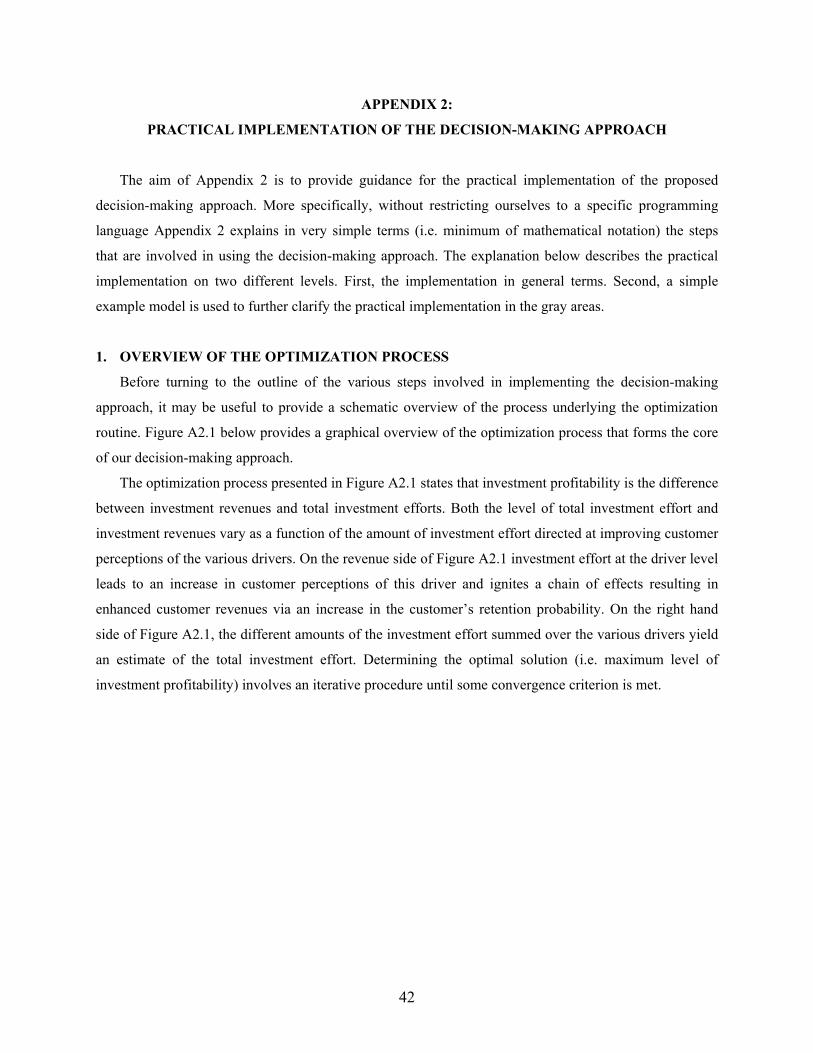
APPENDIX 2:
PRACTICAL IMPLEMENTATION OF THE DECISION-MAKING APPROACH
The aim of Appendix 2 is to provide guidance for the practical implementation of the proposed
decision-making approach. More specifically, without restricting ourselves to a specific programming
language Appendix 2 explains in very simple terms (i.e. minimum of mathematical notation) the steps
that are involved in using the decision-making approach. The explanation below describes the practical
implementation on two different levels. First, the implementation in general terms. Second, a simple
example model is used to further clarify the practical implementation in the gray areas.
1. OVERVIEW OF THE OPTIMIZATION PROCESS
Before turning to the outline of the various steps involved in implementing the decision-making
approach, it may be useful to provide a schematic overview of the process underlying the optimization
routine. Figure A2.1 below provides a graphical overview of the optimization process that forms the core
of our decision-making approach.
The optimization process presented in Figure A2.1 states that investment profitability is the difference
between investment revenues and total investment efforts. Both the level of total investment effort and
investment revenues vary as a function of the amount of investment effort directed at improving customer
perceptions of the various drivers. On the revenue side of Figure A2.1 investment effort at the driver level
leads to an increase in customer perceptions of this driver and ignites a chain of effects resulting in
enhanced customer revenues via an increase in the customer’s retention probability. On the right hand
side of Figure A2.1, the different amounts of the investment effort summed over the various drivers yield
an estimate of the total investment effort. Determining the optimal solution (i.e. maximum level of
investment profitability) involves an iterative procedure until some convergence criterion is met.
42
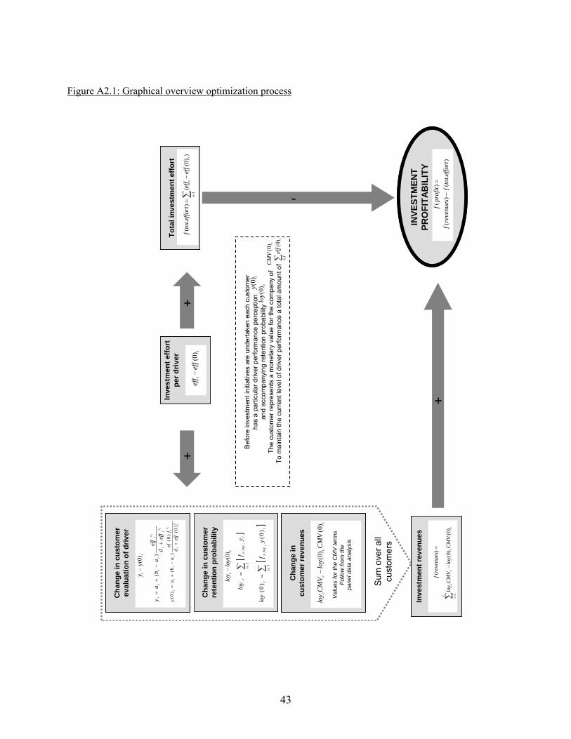
Figure A2.1: Graphical overview optimization process
Sum
ove
r all
cust
omer
s
Inve
stm
ent e
ffort
per d
river
ii
eff
eff
)0(−
Inve
stm
ent e
ffort
per d
river
ii
eff
eff
)0(−
Cha
nge
in c
usto
mer
eval
uatio
n of
driv
er
Cha
nge
in c
usto
mer
rete
ntio
n pr
obab
ility
ii
yy
)0(−
i
i
c ii
c ii
ii
ief
fd
eff
ab
ay
+−
+=
)(
i
i
c ii
c ii
ii
ief
fd
fef
ab
ay
)0()0(
)(
)0(+
−+
=
cc
loy
loy
)0(−
[]
∑ ∈
=I
ii
loy
yc
yf
loy
c,
[]
∑ ∈
=I
ii
loy
yc
yf
loy
c)0(
)0(,
Cha
nge
incu
stom
er re
venu
es
cc
cc
CM
Vlo
yC
MV
loy
)0()0(
−
Val
ues
for t
he C
MV
term
sFo
llow
from
the
pane
l dat
a an
alys
is
Cha
nge
in c
usto
mer
eval
uatio
n of
driv
er
Cha
nge
in c
usto
mer
rete
ntio
n pr
obab
ility
ii
yy
)0(−
i
i
c ii
c ii
ii
ief
fd
eff
ab
ay
+−
+=
)(
i
i
c ii
c ii
ii
ief
fd
fef
ab
ay
)0()0(
)(
)0(+
−+
=
cc
loy
loy
)0(−
[]
∑ ∈
=I
ii
loy
yc
yf
loy
c,
[]
∑ ∈
=I
ii
loy
yc
yf
loy
c)0(
)0(,
Cha
nge
in c
usto
mer
eval
uatio
n of
driv
er
Cha
nge
in c
usto
mer
rete
ntio
n pr
obab
ility
ii
yy
)0(−
i
i
c ii
c ii
ii
ief
fd
eff
ab
ay
+−
+=
)(
i
i
c ii
c ii
ii
ief
fd
fef
ab
ay
)0()0(
)(
)0(+
−+
=
cc
loy
loy
)0(−
[]
∑ ∈
=I
ii
loy
yc
yf
loy
c,
[]
∑ ∈
=I
ii
loy
yc
yf
loy
c)0(
)0(,
Cha
nge
incu
stom
er re
venu
es
cc
cc
CM
Vlo
yC
MV
loy
)0()0(
−
Val
ues
for t
he C
MV
term
sFo
llow
from
the
pane
l dat
a an
alys
is
Cha
nge
incu
stom
er re
venu
es
cc
cc
CM
Vlo
yC
MV
loy
)0()0(
−
Val
ues
for t
he C
MV
term
sFo
llow
from
the
pane
l dat
a an
alys
is
Inve
stm
ent r
even
ues
∑ =
−
=C c
cc
cc
CM
Vlo
yC
MV
loy
reve
nues
f
1)0(
)0(
)(
Inve
stm
ent r
even
ues
∑ =
−
=C c
cc
cc
CM
Vlo
yC
MV
loy
reve
nues
f
1)0(
)0(
)(
Bef
ore
inve
stm
ent i
nitia
tives
are
und
erta
ken
each
cus
tom
erha
s a
parti
cula
r driv
er p
erfo
rman
ce p
erce
ptio
nan
d ac
com
pany
ing
rete
ntio
n pr
obab
ility
The
cust
omer
repr
esen
ts a
mon
etar
y va
lue
for t
he c
ompa
ny o
fTo
mai
ntai
n th
e cu
rrent
leve
l of d
river
per
form
ance
a to
tal a
mou
nt o
f
iy
)0( clo
y)0(
cC
MV
)0(∑ ∈
Ii
ief
f)0(
Tota
l inv
estm
ent e
ffort
))0(
ii
eff
eff−
()
.(
Ii
effo
rtto
tf
=∑ ∈
Tota
l inv
estm
ent e
ffort
))0(
ii
eff
eff−
()
.(
Ii
effo
rtto
tf
=∑ ∈
INVE
STM
).
()
()
(ef
fort
tot
fre
venu
esf
prof
itf
−=EN
TPR
OFI
TAB
ILIT
YIN
VEST
M
).
()
()
(ef
fort
tot
fre
venu
esf
prof
itf
−=EN
TPR
OFI
TAB
ILIT
Y
-+
+
+
43
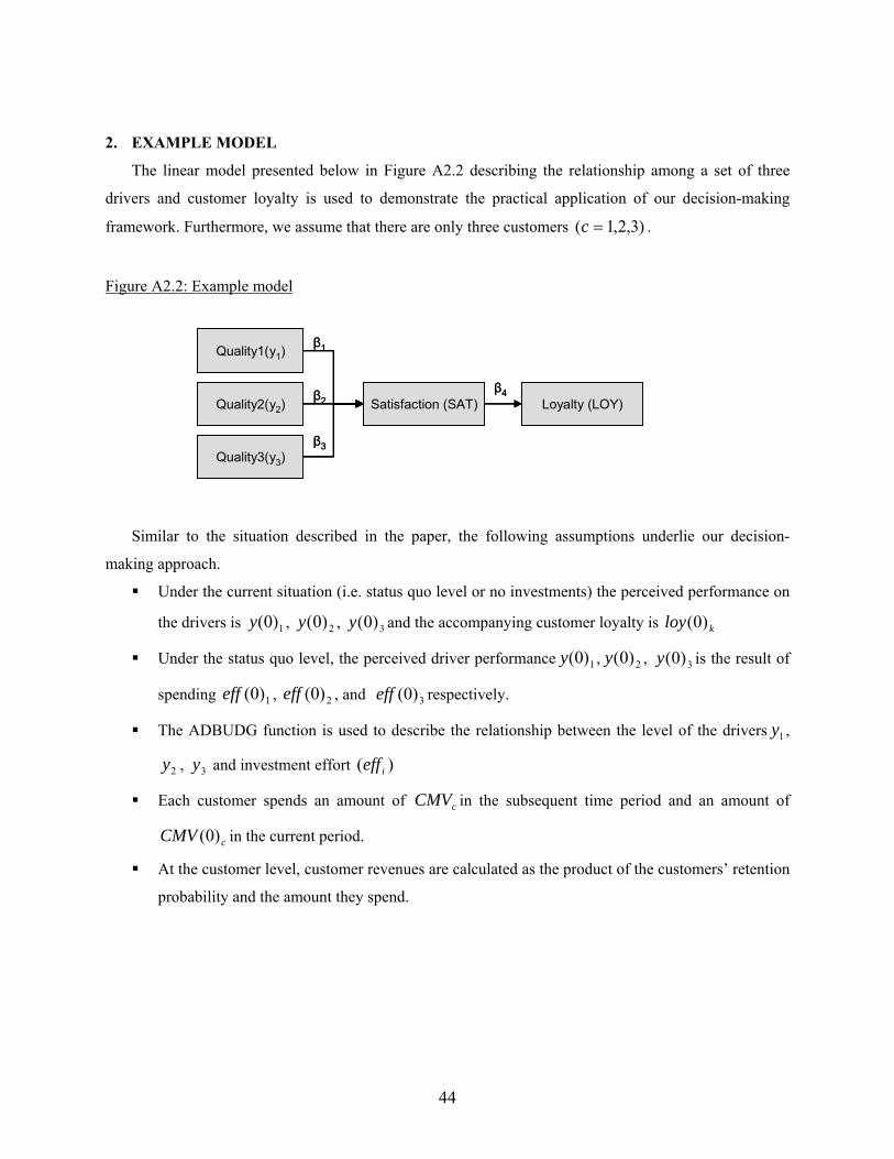
2. EXAMPLE MODEL
The linear model presented below in Figure A2.2 describing the relationship among a set of three
drivers and customer loyalty is used to demonstrate the practical application of our decision-making
framework. Furthermore, we assume that there are only three customers )3,2,1( =c .
Figure A2.2: Example model
Quality1(y1)
Quality2(y2)
Quality3(y3)
Satisfaction (SAT) Loyalty (LOY)
β1
β2
β3
β4
Quality1(y1)
Quality2(y2)
Quality3(y3)
Satisfaction (SAT) Loyalty (LOY)
β1
β2
β3
β4
Similar to the situation described in the paper, the following assumptions underlie our decision-
making approach.
Under the current situation (i.e. status quo level or no investments) the perceived performance on
the drivers is , , and the accompanying customer loyalty is 1)0(y 2)0(y 3)0(y kloy )0(
Under the status quo level, the perceived driver performance , , is the result of
spending , , and respectively.
1)0(y 2)0(y 3)0(y
1)0(eff 2)0(eff 3)0(eff
The ADBUDG function is used to describe the relationship between the level of the drivers ,
, and investment effort
1y
2y 3y )( ieff
Each customer spends an amount of in the subsequent time period and an amount of
in the current period.
cCMV
cCMV )0(
At the customer level, customer revenues are calculated as the product of the customers’ retention
probability and the amount they spend.
44

3. IMPLEMENTATION OF THE OPTIMIZATION PROCESS
The core of our decision-making approach is formed by the optimization process outlined in Figure
A2.1. As with every optimization problem, the aim is to optimize some objective function. In our
framework this is the maximization of the investment profit function. In more formal notation, this can be
summarized as shown in Equation (A2.1a).
Maximize )( profitf (A2.1a)
As the profit function equals the difference between the revenues function and
total investment effort function , an alternative way of expressing the optimization of the
objective function is shown in Equation (A2.1b).
)( profitf )(revenuesf
).( efforttotf
Maximize ).()( efforttotfrevenuesf − (A2.1b)
The procedures needed to define the revenues function and investment effort
function will be outlined in the paragraphs 3.1 and 3.2 respectively.
)(revenuesf
).( efforttotf
3.1 THE REVENUES FUNCTION )f(revenues
The investment revenues per customer are a function of the change in the customer’s retention
probability and the customer’s contribution margin . Furthermore, as each customer already
has a relationship with the firm, we need to model the investment revenues relative to the customer
loyalty probability ( ) and the amount of customer monetary value ) before the
investment initiative is undertaken. Thus, at the level of the individual customer the revenue function is
defined as shown in Equation (A2.2a).
cloy cCMV
cloy )0( cCMV )0((
cccc CMVloyCMVloyrevenuesf )0()0()( −= (A2.2a)
The total investment revenues are determined by summing the revenue function over all c customers.
Thus, in a situation of only three customers as in the example guiding this Appendix the revenue
45

function becomes
))0(())0(())0()0(()(
3333
22221111
CMVloyCMVloyCMVloyCMVloyCMVloyCMVloyrevenuesf
−+−= + −
The terms and in the revenue function are determined as follows. cloy cCMV )(revenuef
3.1.1 Customer monetary value and the revenues function )(revenuef
The figures for the terms and are derived from the internal company data base
containing information on customer contribution margins. For the study at hand, a dynamic regression
model was estimated (see also Equation (A1.3)). The term represents the contribution margin
of customer in the three months before the study and is derived directly from the company data base.
The term represents the expected contribution margin of customer c over the first quarter after the
data collection and is predicted using a panel regression model.
cCMV )0( cCMV
cCMV )0(
c
cCMV
3.1.2 Customer retention probability and the revenues function )(revenuef
Investments aimed at improving customer’s driver perceptions form the starting point to
increasing the customer’s retention probability and thus financial performance. The magnitude of the
relationship between the customer’s retention probability and the different drivers is captured by the term
in the expression (see also Equation (5a) in paper). More specifically,
describes the amount of change in the customer retention probability caused by changes in
variable . The term equals the product of the marginal effects for each path connecting and
and subsequently summing these products over all relevant paths connecting and loy . See also
Appendix 1 Equations (A1.1)-(A1.2) for the exact calculation.
loyyif ∑
∈
=Ii
iloyy yfloyi
loyyif
iy loyyif iy
loy iy
The values for stems from the survey data and are customer c ’s evaluations of the relevant
input variables. Note that the values for typically vary across customers.
iy )0(
iy )0(
The (optimal) value for needed to calculate the customer retention probability and revenues is
determined during the optimization analysis as a function of the level of investment effort . The exact
nature of the relationship between and is captured by the ADBUDG function.
iy
ieff
iy ieff
46

For the example model which contains only linear relationships the term boils down to loyyif
∑∈Ii
ii yλ where iλ is the relation between the thi − driver and the customer retention
probability . Applying Equations (1.1) and (1.2) to the coefficients in Figure (A2.2) leads cloy
to: 411 ββλ = , 422 ββλ = , and 433 ββλ = .
As such, the terms loy and in revenues function can be written respectively )0(loy )(revenuesf
as 3322 y11 yyloy λ λλ ++= and 332211 )0()0()0()0( yyyloy λλλ ++= where the term
differs per customer depending the customer’s driver perceptions . 321 )0(,)0(,)0( yyy)0(loy
3.2 The investment effort function rt)f(tot.effo
The ADBUDG function is the foundation for the investment effort function . For
each driver the ABDUDG function needs to be calibrated to describe the link between the customer’s
perceptions of the relevant driver ( ) and the amount of investment effort ( ) needed to improve the
particular driver. The various ADBUDG parameters are calibrated using the procedure outlined in
Appendix 1. The amount of total investment reflected by function equals the sum of
different amounts of investment directed to the various drivers .
).( efforttotf
iy
iy ieff
).( efforttotf
ieff iy
In terms of the example model this implies that three effort functions are specified. That is, for
each driver a separate ADBUDG function is needed.
1
1
11
11111 )( c
c
effdeffabay+
−+=
2
2
22
22222 )( c
c
effdeffabay+
−+=
3
3
33
33333 )( c
c
effdeff
abay+
−+=
Furthermore, the function for the total level of investment effort is
321).( effeffeffefforttotf ++=
3.3 The constraints
47

Specification of the constraints ensures that the relationships of the optimization analysis follow
the predetermined structure. More particularly, we impose the following constraints.
3.3.1 Constraint 1
Constraint that describes the nature of the relationship between the drivers and the customer
retention probability. This constraint reflects the theoretical framework underlying the nomological web
of relations among the input variables and the retention probability . For the situation at hand, this
constraint is summarized as .
iy cloy
[ ]∑∈
=Ii
iloyyc yfloyci ,
3.3.2 Constraint 2
Constraint that describes the nature of the relationship between the level of the input variables
and the amount of investment effort directed at them. This constraint equals the ADBUDG function for
the different drivers.
3.3.3 Constraint 3
Budget constraint that states that the available amount of total investment effort is capped by a
pre-determined maximum or budget B . Note that this constraint may be relaxed by setting the budget
B equal to infinity. This constraint is formally denoted as Befforttotf ≤).( or equivalently ∑∈
≤Ii
i Beff
3.3.4 Constraint 4
Constraint that restricts the level of investment effort to a minimum value of zero. That is,
minimum of investment effort directed to a driver is zero. More formally, . ieff iy 0≥ieff
Overall, the decision-making framework for the example in this Appendix can be summarized as follows.
Maximize
( ) ( ) ( )( )332211
333322221111
)0(())0(())0()0()0()0()0()0()0(
effeffeffeffeffeffCMVloyCMVloyCMVloyCMVloyCMVloyCMVloy
−+−+−−+− − + −
Subject to:
48

Constraint 1
343242141 yyyloy ββ β β ++= β β
Constraint 2
1
1
11
11111 )( c
c
effdeffabay+
−+=
2
2
22
22222 )( c
c
effdeffabay+
−+=
3
3
33
33333 )( c
c
effdeff
abay+
−+=
Constraint 3
( ) ( ) ( ) Budgeteffeffeffeffeffeff −+−+− 332211 )0()0()0( ≤
Constraint 4
0))0(( 11 ≥− effeff
0))0(( 22 ≥− effeff
0))0(( 33 ≥− effeff
4. CONDUCTING THE OPTIMIZATION ANALYSIS
This section provides an overview of how the different analysis stemming from our optimization
approach can be conducted.
4.1 Optimal level of investment effort
This type of analysis can be performed in two ways. The most appropriate way is by determining
the derivative of the profit function with respect to investment effort, setting this derivative equal to zero,
and having the program solve this equation. As shown in Appendix 1 this often involves a long and
complex derivation. An alternative way to determining the optimal level of investment effort is by
running the optimization framework for a series of different budgets and manually look for the optimum
level of investment effort. In particular, plotting the profitability levels against the budgets then provides a
simple way to find the optimal investment effort level (see also for example Figure 2 in the paper).
49

4.2 Optimal allocation of investment effort
Running the optimization analysis with the optimal investment effort level as budget constraint
provides a solution containing the optimal effort level per driver. The solution contains values for both
and . It may be convenient to express the allocation of investment effort in relative terms. To do this,
calculate the fraction ( )
iy
ieff
( )∑∈
−−Ii
iiii effeffeffeff )0(/)0( for each driver. Finally, use the data to calibrate
the ADBUDG function to derive the actual investment action corresponding with the optimal effort levels
per driver.
4.3 Return on investment
The investment effort level and the resulting profitability level stemming from the optimization
analysis provide sufficient information to calculate the rate of return on investment expressed by Equation
(9) in the paper.
4.4 Robustness of the optimal solution
Nominal range sensitivity analysis involves examining how the optimal solution changes as a
result of altering a single parameter in the model while keeping the other parameters at their base-case
values. Nominal range sensitivity analysis for the model parameters linking the drivers to the customer
retention probability (i.e. part of ) proceeds as follows. )(revenuesf
First, use the total profitability level (i.e. including the profitability at the status quo level) of the
original optimal solution as a baseline for comparison. Second, determine the consequences of a change
in a single model parameter using Equation (A1.7). Third, determine the level of total profitability that
would be obtained under the original optimal investment level allocation taking into the changed model
parameter. Fourth, determine the relative change in projected investment profitability as described in
Appendix 1.
It should be noted that a similar procedure may also be performed on the functions related to the
investment effort.
Original optimal solution is based on parameters 14λ , 24λ , and 34λ and spending
amounts , , and to the respective drivers. This yields an optimal profit level of 1eff 2eff 3eff
)()(),,( 321343242141342414 effeffeffyyyprofit ++−++= λλλλλλ .
As we assume that the cost function remains stable, the driver levels resulting from the optimal
50

allocation scheme are unaffected by changes in the customer retention model. To assess the
robustness of the optimal profitability level as the different parameters would alter by δ we
proceed as follows.
Path between Qual1( ) and Satisfaction ( ) 1y SAT
If parameter 1β increases withδ , resulting into δβ +1 , 4114 ββλ = changes to
44141'14 )( δββββδβλ +=+= (see also Equation (A1.7)). This will in turn yield a profit level
of )()(),,( 321343242'1413424
'14 effeffeffyyyprofit ++−++= λλλλλλ
Path between Qual2( ) and Satisfaction ( ) 2y SAT
If parameter 2β increases withδ , resulting into δβ +2 , 4224 ββλ = changes to
44242'24 )( δββββδβλ +=+= (see also Equation (A1.7)). This will in turn yield a profit level
of )()(),,( 321343'24214134
'2414 effeffeffyyyprofit ++−++= λλλλλλ
Path between Qual3( ) and Satisfaction ( ) 3y SAT
If parameter 3β increases withδ , resulting into δβ +3 , 4334 ββλ = changes to
44343'34 )( δββββδβλ +=+= (see also Equation (A1.7)). This will in turn yield a profit level
of )()(),,( 321'343242141
'342414 effeffeffyyyprofit ++−++= λλλλλλ
Path between Satisfaction ( ) and Loyalty ( SAT )LOY
An increase in parameter 4β withδ , resulting into δβ +4 , has consequences for the relationships
among each of the quality variables and . More specifically, the impact of on 1y 2y 3y LOY 1y
LOY changes from 4114 ββλ = into ; impact of on 14141'14 )( δβββδββλ +=+= 2y LOY
changes from 4224 ββλ = into ; and the impact of on 24242'24 )( δβββδββλ +=+= 3y LOY
changes from 4334 ββλ = into . 34343'34 )( δβββδββλ +=+=
With as the accompanying )()(),,( 321'343
'242
'141
'34
'24
'14 effeffeffyyyprofit ++−++= λλλλλλ
profitability level.
51

Now, compare the new level of profitability with original optimal level of profitability for each of
the changed parameters.
Path between Qual1( ) and Satisfaction ( ) 1y SAT
%100*),,(
),,(),,(
342414
3424143424'14
⎟⎟⎠
⎞⎜⎜⎝
⎛ −λλλ
λλλλλλprofit
profitprofit
Path between Qual2( ) and Satisfaction ( ) 2y SAT
%100*),,(
),,(),,(
342414
34241434'2414
⎟⎟⎠
⎞⎜⎜⎝
⎛ −λλλ
λλλλλλprofit
profitprofit
Path between Qual3( ) and Satisfaction ( ) 3y SAT
%100*),,(
),,(),,(
342414
342414'342414
⎟⎟⎠
⎞⎜⎜⎝
⎛ −λλλ
λλλλλλprofit
profitprofit
Path between Satisfaction ( ) and Loyalty ( SAT )LOY
%100*),,(
),,(),,(
342414
342414'34
'24
'14
⎟⎟⎠
⎞⎜⎜⎝
⎛ −λλλ
λλλλλλprofit
profitprofit
52
REFERENCES
Ahuja, R.K., Magnanti, T.L., & Orlin, J.B. (1993). Network Flows: Theory, Algorithms, and
Applications. Englewood Cliffs, NJ: Prentice Hall.
Anderson, E.W., Fornell, C., & Lehmann, D.R. (1994). Customer satisfaction, market share, and
profitability: findings from Sweden. Journal of Marketing, 58(3), 53-66.
Anderson, E.W., & Sullivan, M.W. (1993). Antecedents and consequences of customer
satisfaction for firms. Marketing Science, 12(2), 107-120.
Baltagi, B.H. (2008). Econometric Analysis of Panel Data. Chichester (UK): John Wiley & Sons
Ltd.
Blattberg, R., Getz, G., & Thomas, J.S. (2001). Customer Equity: Building and Managing
Relationships as Valuable Assets. Boston, MA: Harvard Business School Press.
Blattberg, R.C., & Hoch, S.J. (1990). Database models and managerial intuition: 50% model +
50% manager. Management Science, 36(8), 887-899.
Bolton, R.N. (1998). A dynamic model of the duration of the customer’s relationship with a
continuous service provider. Marketing Science, 17 (1), 45-65.
Bolton, R.N., & Drew, J.H. (1991). A multistage model of customers’ assessment of service
quality and value. Journal of Consumer Research, 17 (4), 875-884.
Boudreau, J., Hopp, W, McClain, J.O., & Thomas, L.J. (2003). On the interface between
operations management and human resource management. Management Science, 5(3),
179-202.
Brealey, R.A., & Myers, S.C. (2000). Principles of corporate finance. New York, NY: McGraw-
Hill College.
53
Bretthauer, K.M. (2004). Service management. Decision Sciences, 35(3), 325-332.
Cronin, J.J., Jr., Brady, M.K., & Hult, G.T. (2000). Assessing the effects of quality, value, and
customer satisfaction on consumer behavioral intentions in service environments. Journal
of Retailing, 76(2), 193-218.
Diamantopoulos, A., & Winklhofer, H.M. (2001). Index construction with formative indicators:
an alternative to scale development. Journal of Marketing Research, 38(2), 269-277.
Dodds, W.B., Monroe, K.B., & Grewal, D. (1991). Effects of price, brand, and store information
on buyers’ product evaluations. Journal of Marketing Research, 28(3), 307-319.
Dong, W., Swain, S.D., & Berger, P.D. (2007). The role of channel equity in customer equity
management. Journal of Business Research, 60 (12), 1243-1252.
Fornell, C., & Wernerfelt, B. (1987). Defensive marketing strategy by customer complaint
management: A theoretical analysis. Journal of Marketing Research, 24(4), 337-346.
Fornell, C., & Wernerfelt, B. (1988). A model for customer complaint management. Marketing
Science, 7(3), 287-298.
Frey, H.C., & Patil, S.R. (2002). Identification and review of sensitivity analysis methods. Risk
Analysis: An International Journal, 22(3), 533-578.
Ganesan, S. (1994). Determinants of long-term orientation in buyer-seller relationships. Journal
of Marketing, 58(2), 1-19.
Garbarino, E., & Johnson, M.S. (1999). The different roles of satisfaction, trust, and commitment
in customer relationships. Journal of Marketing, 63(2), 70-87.
54
Gök, O. (2008). Linking account portfolio management to customer information: using customer
satisfaction metrics for portfolio analysis. Industrial Marketing Management,
forthcoming.
Gounaris, S.P. (2005). Trust and commitment influences on customer retention: insights from
business-to-business services. Journal of Business Research, 58 (2), 126-140.
Gwinner, K.P., Gremler, D.D., & Bitner, M.J. (1998). Relational benefits in service industries:
the customer’s perspective. Journal of the Academy of Marketing Science, 26 (2), 101-
114.
Han, S., & Sung, H. (2008). Industrial brand value and relationship performance in business
markets – a general structural equation model. Industrial Marketing Management, 37 (7),
807-818.
Keh, H.T., & Xie, Y. (2008). Corporate reputation and customer behavioral intentions: The roles
of trust, identification, and commitment. Industrial Marketing Management, forthcoming.
Kumar, V. & George, M. (2007). Measuring and maximizing customer equity: a critical analysis.
Journal of the Academy of Marketing Science, 35 (2), 157-171.
Kumar, N., Scheer, L.K., & Steenkamp, J.B.E.M. (1995). The effects of perceived
interdependence on dealer attitudes. Journal of Marketing Research, 32(3), 348-356.
Lam, S.Y., Shankar, V., Erramilli, M., & Murthy, B. (2004). Customer value, satisfaction,
loyalty, and switching costs: an illustration from a business-to-business service context.
Journal of the Academy of Marketing Journal, 32 (3), 293-311.
LaPlaca, P.J. (2004). Special issue on customer relationship management. Industrial Marketing
Management, 33 (6), 463-464.
55

Lewin, J.E. (2008). Business customers’ satisfaction: what happens when suppliers downsize?
Industrial Marketing Management, forthcoming.
Little, J.D.C. (1970). Models and managers: the concept of a decision calculus. Management
Science, 16(8), 466-485.
MacKenzie, S.B., Podsakoff, P.M., & Jarvis, C.B. (2005). The problem of measurement model
misspecification in behavioral and organizational research and some recommended
solutions. Journal of Applied Psychology, 90 (4), 710–30.
Mantrala, M.K., Sinha, P., & Zoltners, A.A., (1992). Impact of resource allocation rules on
marketing investment-level decisions and profitability. Journal of Marketing Research,
29(2), 162-175.
Metters, R., & Marucheck, A. (2007). Service management – Academic issues and scholarly
reflections from operations management researchers. Decision Sciences, 38(2), 195-214.
Morgan, M.G., & Henrion, M. (1990). Uncertainty: a guide to dealing with uncertainty in
quantitative risk and policy analysis. Cambridge, NY: Cambridge University Press.
Nijssen, E., Singh, J., Sirdeshmukh, D., & Holzmueller, H. (2003). Investigating industry context
effects in consumer-firm relationships: Preliminary results from a dispositional approach.
Journal of the Academy of Marketing Science, 31(1), 46-60.
Oliver, R.L. (1999). Whence consumer loyalty? Journal of Marketing, 63 (4), 33-44.
Roncek, D.W. (1993). When will they ever learn that first order derivative identify the effects of
continuous independent variables or “Officer, you can’t give me a ticket, I wasn’t
speeding for an entire hour”. Social Forces, 71(4), 1067-1078.
56
Rust, R.T., Lemon, K.N., & Zeithaml, V.A. (2004). Return on marketing: using customer equity
to focus marketing strategy. Journal of Marketing, 68(1), 109-127.
Rust, R.T., Moorman, C., & Dickson, P.R. (2002). Getting returns on quality: revenue
expansion, cost reduction, or both?. Journal of Marketing, 66(4), 7-24.
Rust, R.T., Zahorik, A.J., & Keiningham, T.L. (1995). Return on quality (ROQ): making service
quality financially accountable. Journal of Marketing, 59(2), 58-70.
Seggie, S.H., Cavusgil, E., & Phelan, S.E. (2007). Measurement of return on marketing
investment: a conceptual framework and the future of marketing metrics. Industrial
Marketing Management, 36 (6), 834-841.
Selnes, F. (1998). Antecedents and consequences of trust and satisfaction in buyer-seller
relationships. European Journal of Marketing, 32 (3/4), 305-322.
Singh, J., & Sirdeshmukh, D. (2000). Agency and trust mechanisms in consumer satisfaction and
loyalty judgments. Journal of the Academy of Marketing Science, 28(1), 150-167.
Sweeney, J.C., Soutar, G.N., & Johnson, L.W. (1999). The role of perceived risk in the quality-
value relationship: a study in a retail environment. Journal of Retailing, 75 (1), 77-105.
Tenenhaus, M., Esposito Vinzi, V., Chatelin, Y.M., & Lauro, C. (2005). PLS path modeling,
Computational Statistics & Data Analysis, 48(1), 159-205.
Venkatesan, R., & Kumar, V. (2004). A customer lifetime value framework for customer
selection and resource allocation strategy. Journal of Marketing, 68 (4), 106-125.
von Winterfelt, D., & Edwards, W. (1986). Decision analysis and behavioral research.
Cambridge, NY: Cambridge University Press.
57
Wooldridge, J.M. (2002) Econometric Analysis of Cross Section and Panel Data. Cambridge,
MA: The MIT Press.
Zeithaml, V.A. (1988). Consumer perceptions of price, quality, and value: a means-end model
and synthesis of evidence. Journal of Marketing, 52(3), 2-21.
Zeithaml, V.A. (2000). Service quality, profitability and the economic worth of customers: what
we know and what we need to learn. Journal of the Academy of Marketing Science, 28(1)
67-85.
Zhu, Z., Sivakumar, K., & Parasuraman, A. (2004). A mathematical model of service failure and
recovery strategy. Decision Sciences, 35(3), 493-525.
58

Table 1: Literature overview relationship dynamics
Relationship Literature in support of the hypothesized relationship
QUAL → VALUE Cronin et al. (2000); Sweeney et al. (1999); Bolton and Drew (1991)
QUAL → SAT Lewin (2008); Cronin et al. (2000); Bolton (1998); Anderson and Sullivan (1993)
VALUE → SAT Lewin (2008); Lam et al. (2004); Cronin et al. (2000)
SAT→ TRUST Selnes (1998); Ganesan (1994)
QUAL → TRUST Singh and Sirdeshmukh (2000); Gounaris (2005)
VALUE → SAT Lewin (2008); Lam et al. (2004)
VALUE → TRUST Gwinner et al. (1998)
SAT → LOY Lewin (2008); Lam et al. (2004); Anderson and Sullivan (1993)
TRUST → LOY Keh and Xie (2008) Garbarino and Johnson (1999), Singh and Sirdeshmukh (2000)
QUAL → LOY Nijssen et al. (2003), Cronin et al. (2000)
VALUE → LOY Lam et al. (2004); Cronin et al. (2000)
59

Table 2: Descriptive statistics and psychometric properties
1 2
3 4
5 6
7 8
9 10
11
12
13
14
15
16
17
18
1
QU
AL
1 1
2
QU
AL
2 0.
56
1
3
QU
AL
3 0.
34
0.36
1
4
QU
AL
4 0.
42
0.37
0.
23
1
5
QU
AL
5 0.
39
0.54
0.
35
0.32
1
6
QU
AL
6 0.
33
0.39
0.
32
0.34
0.
41
1
7
QU
AL
7 0.
43
0.37
0.
23
0.26
0.
39
0.43
1
8
SAT
0.
48
0.55
0.
31
0.33
0.
57
0.48
0.
45
1
9
VA
LU
E1
0.23
0.
23
0.13
0.
14
0.14
0.
20
0.17
0.
30
1
10
VA
LU
E2
0.30
0.
35
0.13
0.
24
0.32
0.
25
0.25
0.
41
0.66
1
11
VA
LU
E3
0.27
0.
26
0.16
0.
29
0.24
0.
18
0.25
0.
36
0.59
0.
55
1
12
VA
LU
E4
0.20
0.
26
0.17
0.
23
0.35
0.
21
0.20
0.
37
0.45
0.
46
0.45
1
13
TR
UST
1 0.
22
0.22
0.
14
0.18
0.
18
0.18
0.
22
0.33
0.
47
0.47
0.
41
0.33
1
14
T
RU
ST2
0.15
0.
23
0.22
0.
12
0.15
0.
11
0.14
0.
36
0.32
0.
33
0.36
0.
20
0.56
1
15
TR
UST
3 0.
17
0.29
0.
05
0.15
0.
23
0.14
0.
16
0.35
0.
40
0.41
0.
39
0.29
0.
59
0.57
16
TR
UST
4 0.
16
0.23
0.
21
0.24
0.
16
0.13
0.
09
0.30
0.
29
0.33
0.
31
0.19
0.
60
0.58
0.
617
T
RU
ST5
0.13
0.
31
0.12
0.
19
0.21
0.
12
0.16
0.
37
0.45
0.
45
0.45
0.
35
0.64
0.
57
0.7
18
()
0.20
0.
26
0.07
0.
27
0.29
0.
04
0.18
0.
36
0.25
0.
32
0.38
0.
28
0.32
0.
23
0.3
1
1
1
2
0.68
1
P
LO
Y4
0.24
0.
41
1
ME
AN
7.
82
7.61
6.
97
7.50
7.
50
7.52
7.
49
8.76
8.
20
8.47
8.
68
6.85
8.
58
7.44
8.
63
7.75
8.
33
0.72
S.D
. 0.
64
0.71
0.
91
0.97
0.
70
0.88
0.
80
0.68
1.
95
2.30
2.
07
3.30
2.
28
2.48
2.
13
2.39
2.
22
0.23
LO
AD
ING
0.
70
0.80
0.
44
0.54
0.
82
0.67
0.
64
n.a.
0.
74
0.87
0.
83
0.72
0.
83
0.77
0.
85
0.82
0.
89
n.a.
LO
WE
R B
OU
ND
0.
56
0.69
0.
22
0.32
0.
70
0.53
0.
48
n.a.
0.
57
0.74
0.
71
0.54
0.
76
0.68
0.
78
0.73
0.
84
n.a.
UPP
ER
BO
UN
D
0.82
0.
90
0.65
0.
73
0.91
0.
80
0.78
n.
a.
0.86
0.
86
0.92
0.
96
0.88
0.
83
0.89
0.
87
0.92
n.
a.
1ST
EIG
EN
VA
LU
E
n.a.
n.
a.
2.59
3.46
n.
a.
2N
D E
IGE
NV
AL
UE
n.
a.
n.a.
0.
62
0.
48
n.a.
CR
ON
BA
CH
’S α
n.
a.
n.a.
0.
78
0.
89
n.a.
AV
E
n.a.
n.
a.
0.63
0.69
n.
a.
60

Table 3: Empirical results structural model
Relationship Unstandardized coefficient
Standardized coefficient
Bias corrected bootstrap percentile confidence interval
Adjusted R2 bootstrap percentile confidence interval
QUAL → VAL 0.595 0.446 [0.259;0.534] VAL: R2 (adj)=0.199*
QUAL → SAT 0.763 0.606 [0.476;0.702] VAL → SAT 0.181 0.192 [0.069;0.327] SAT: [0.489;0.508] QUAL → TRUST Not significant Not significant Not significant VAL → TRUST 0.436 0.448 [0.281;0569] SAT → TRUST 0.208 0.202 [0.089;0.326] TRUST: [0.309;0.325] QUAL → P(LOY) Not significant Not significant Not significant VAL → P(LOY) 0.993 0.277 [0.097;0.435] SAT → P(LOY) 0.558 0.147 [0.006;0.300] TRUST → P(LOY) 0.999 0.271 [0.098;0.326] P(LOY): [0.288;0.323] * As VAL is a function of just an endogenous construct it is not possible to construct a bootstrap percentile confidence interval for its R2 (adj) value.
61

Table 4: Empirical results dynamic regression analysis
Independent
variables
Explanation dummy variables Unstandardized
coefficient
t-value (p-value)
1, −tcCMV 0.30 6.60 (p<0.0001)
2, −tcQUANT 0.64 23.06 (p<0.000
cSIZE1 Compares size quartiles 1 and 2 1652 3.00 (p=0028)
cSIZE2 Compares size quartile 1 and 3 6929 9.13 (p<0.0001)
cTYPE1 Compares user of product line B to
those of product line A
n.s.
cTYPE2 Compares used of product lines A and
B to those of product line A
n.s.
cREL n.s.
1)
62
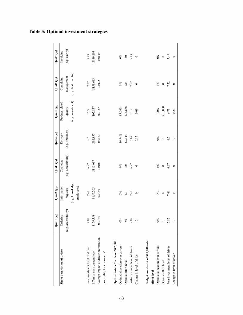
Table 5: Optimal investment strategies
Q
ual1
(y1)
Q
ual2
(y2)
Q
ual3
(y3)
Q
ual4
(y4)
Q
ual5
(y5)
Q
ual6
(y6)
Q
ual7
(y7)
Shor
t des
crip
tion
of d
rive
r O
rder
ing
(e.g
. acc
essi
bilit
y)
Info
rmat
ion
requ
ests
(e.g
. kno
wle
dge
empl
oyee
s)
Cat
alog
ue
(e.g
. acc
essi
bilit
y)
Del
iver
y
(e.g
. tim
elin
ess)
Prod
uct r
elat
ed
qual
ity
(e.g
. ass
ortm
ent)
Com
plai
nt
man
agem
ent
(e.g
. firs
t tim
e fix
)
Invo
icin
g
(e.g
. cla
rity)
Pre-
inve
stm
ent l
evel
of d
river
7.
82
7.61
6.
97
6.5
6.5
Effo
rt to
mai
n cu
rren
t lev
el
$179
,358
$1
59,2
05
$115
,017
$9
2,85
7 $9
2,85
7
Ave
rage
impa
ct o
f driv
er o
n re
tent
ion
prob
abili
ty fo
r cus
tom
er c
0.01
64
0.01
91
0.01
03
0.01
33
0.01
87
Opt
imal
tota
l eff
ort l
evel
$42
,000
Opt
imal
allo
catio
n ov
er d
river
s 0%
0%
0%
16
.94%
83
.06%
Opt
imal
eff
ort l
evel
$0
$0
$0
$7
,114
$3
4,88
6
Post
-inve
stm
ent l
evel
of d
river
7.
82
7.61
6.
97
6.67
7.
19
7.52
7.
49
$151
,613
$1
49,2
03
0.01
35
0.01
49
0%
0%
$0
$0
7.
52
7.49
Cha
nge
in le
vel o
f driv
er
0 0
0 0.
17
0.69
0
0
Bud
get c
onst
rain
t of $
10,0
00 to
tal
effo
rt le
vel
Opt
imal
allo
catio
n ov
er d
river
s 0%
0%
0%
0%
10
0%
0%
0%
Opt
imal
eff
ort l
evel
0
0 0
0 $1
0,00
0 0
0
Post
-inve
stm
ent l
evel
of d
river
7.
82
7.61
6.
97
6.5
6.73
7.
52
7.49
Cha
nge
in le
vel o
f driv
er
0 0
0 0
0.23
0
0
63

Table 6: Sensitivity analysis
wij
- 5%
w
ij + 5
%
Inve
stm
ent
Inve
stm
ent
Path
pr
ofita
bilit
y Δ%
R
OI (
%)
prof
itabi
lity
Δ
%
R
OI (
%)
Qua
l1 →
Qua
lity
$ 11
,984
35
28
.51
$ 4,
136
53
9.85
Q
ual2
→Q
ualit
y $
11,7
94
33
28.0
8 $
6,23
0 30
14
.83
Qua
l3 →
Qua
lity
$ 10
,196
15
24
.28
$ 7,
640
14
18.1
9 Q
ual4
→Q
ualit
y $
10,5
96
19
25.2
3 $
7,28
6 18
17
.35
Qua
l5 →
Qua
lity
$ 9,
614
8 22
.89
$ 8,
185
8 19
.49
Qua
l6 →
Qua
lity
$ 10
,969
23
26
.12
$ 6,
940
22
16.5
2 Q
ual7
→Q
ualit
y $
11,0
18
24
26.2
3 $
6,90
0 22
16
.43
Qua
lity →
Val
ue
$ 16
,982
91
40
.43
$ 2,
594
71
6.18
Q
ualit
y →
Sat
isfa
ctio
n $
15,6
17
76
37.1
8 $
3,92
9 56
9.
35
Val
ue →
Sat
isfa
ctio
n $
14,1
24
59
33.6
3 $
4,69
1 47
11
.17
Satis
fact
ion→
Tru
st
$ 10
,429
17
24
.83
$ 6,
730
24
16.0
2 V
alue
→ T
rust
$
14,2
70
61
33.9
8 $
3,93
8 56
9.
38
Val
ue →
Loy
alty
$
13,5
56
53
32.2
8 $
4,58
0 48
10
.90
Satis
fact
ion →
Loy
alty
$
14,4
47
63
34.4
0 $
2,94
5 67
7.
01
Trus
t → L
oyal
ty
$ 15
,900
79
37
.86
$ 3,
238
64
7.71
64
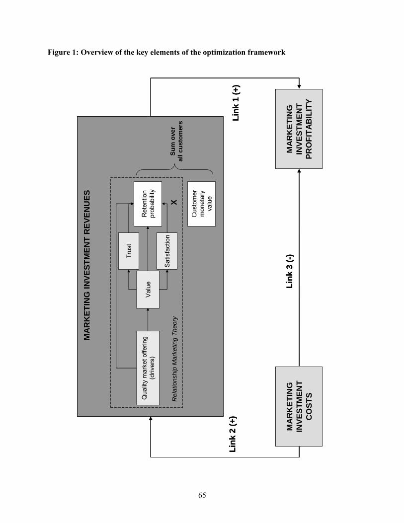
Figure 1: Overview of the key elements of the optimization framework
MA
RK
ETIN
GIN
VEST
MEN
TPR
OFI
TAB
ILIT
Y
MA
RK
ETIN
G IN
VEST
MEN
T R
EVEN
UES
Ret
entio
npr
obab
ility
Cus
tom
erm
onet
ary
valu
eX
Trus
t
Sat
isfa
ctio
n
Val
ueQ
ualit
y m
arke
t offe
ring
(driv
ers)
Sum
oal
l cus
ver
tom
ers
Rel
atio
nshi
p M
arke
ting
Theo
ry
MA
RK
ETIN
G IN
VEST
MEN
T R
EVEN
UES
Ret
entio
npr
obab
ility
Cus
tom
erm
onet
ary
valu
eX
Trus
t
Sat
isfa
ctio
n
Val
ueQ
ualit
y m
arke
t offe
ring
(driv
ers)
Sum
oal
l cus
ver
tom
ers
Rel
atio
nshi
p M
arke
ting
Theo
ry
Link
1 (+
)
Link
3 (-
)M
AR
KET
ING
INVE
STM
ENT
PRO
FITA
BIL
ITY
MA
RK
ETIN
GIN
VEST
MEN
TC
OST
S
Link
2 (+
)
MA
RK
ETIN
G IN
VEST
MEN
T R
EVEN
UES
Ret
entio
npr
obab
ility
Cus
tom
erm
onet
ary
valu
eX
Trus
t
Sat
isfa
ctio
n
Val
ueQ
ualit
y m
arke
t offe
ring
(driv
ers)
Sum
oal
l cus
ver
tom
ers
Rel
atio
nshi
p M
arke
ting
Theo
ry
MA
RK
ETIN
G IN
VEST
MEN
T R
EVEN
UES
Ret
entio
npr
obab
ility
Cus
tom
erm
onet
ary
valu
eX
Trus
t
Sat
isfa
ctio
n
Val
ueQ
ualit
y m
arke
t offe
ring
(driv
ers)
Sum
oal
l cus
ver
tom
ers
Rel
atio
nshi
p M
arke
ting
Theo
ry
Link
1 (+
)
Link
3 (-
)M
AR
KET
ING
INVE
STM
ENT
CO
STS
Link
2 (+
)
65
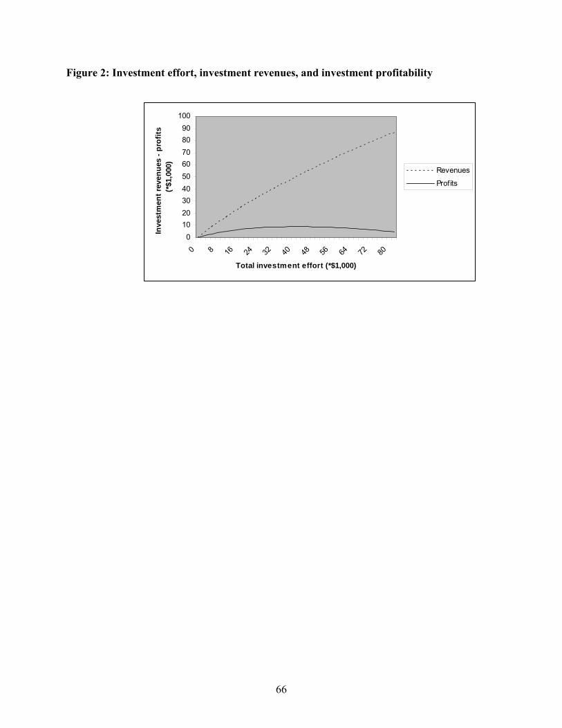
Figure 2: Investment effort, investment revenues, and investment profitability
0102030405060708090
100
0 8 16 24 32 40 48 56 64 72 80
Total investment effort (*$1,000)
Inve
stm
ent r
even
ues
- pro
fits
(*$1
,000
)Revenues
Profits
66