1

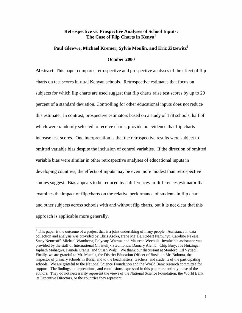
Retrospective vs. Prospective Analyses of School Inputs:The Case of Flip Charts in Kenya1

Paul Glewwe, Michael Kremer, Sylvie Moulin, and Eric Zitzewitz2

October 2000

Abstract: This paper compares retrospective and prospective analyses of the effect of flip

charts on test scores in rural Kenyan schools. Retrospective estimates that focus on

subjects for which flip charts are used suggest that flip charts raise test scores by up to 20

percent of a standard deviation. Controlling for other educational inputs does not reduce

this estimate. In contrast, prospective estimators based on a study of 178 schools, half of

which were randomly selected to receive charts, provide no evidence that flip charts

increase test scores. One interpretation is that the retrospective results were subject to

omitted variable bias despite the inclusion of control variables. If the direction of omitted

variable bias were similar in other retrospective analyses of educational inputs in

developing countries, the effects of inputs may be even more modest than retrospective

studies suggest. Bias appears to be reduced by a differences-in-differences estimator that

examines the impact of flip charts on the relative performance of students in flip chart

and other subjects across schools with and without flip charts, but it is not clear that this

approach is applicable more generally.

1 This paper is the outcome of a project that is a joint undertaking of many people. Assistance in datacollection and analysis was provided by Chris Asoka, Irene Majale, Robert Namunyu, Caroline Nekesa,Stacy Nemeroff, Michael Wambetsa, Polycarp Waswa, and Maureen Wechuli. Invaluable assistance wasprovided by the staff of International Christelijk Steunfonds: Damary Alembi, Chip Bury, Jos Huizinga,Japheth Mahagwa, Pamela Oranja, and Susan Walji. We thank our discussant at Stanford, Ed Vytlacil.Finally, we are grateful to Mr. Munala, the District Education Officer of Busia, to Mr. Buluma, theinspector of primary schools in Busia, and to the headmasters, teachers, and students of the participatingschools. We are grateful to the National Science Foundation and the World Bank research committee forsupport. The findings, interpretations, and conclusions expressed in this paper are entirely those of theauthors. They do not necessarily represent the views of the National Science Foundation, the World Bank,its Executive Directors, or the countries they represent.

2

Introduction

Most analyses of the effect of educational inputs are based on retrospective

studies, which compare schools with different levels of inputs (Hanushek, 1995). One

potential weakness of this approach is that observed inputs may be correlated with

omitted variables that affect educational outcomes. This could potentially bias outcomes

in either direction. For example, if parents who provide better home environments for

children tend to organize politically to obtain more school inputs for their children,

estimates of the effect of these school inputs on test scores may be biased upwards. On

the other hand, if compensatory programs provide schools in disadvantaged areas with

additional inputs, then retrospective studies may underestimate the effect of these inputs.

The direction and severity of these biases is ultimately an empirical question. This paper

compares retrospective and prospective estimates of the effects of flip charts in Kenyan

primary schools.3 We find that prospective estimates are much smaller than retrospective

estimates, suggesting that retrospective estimates are subject to serious upward omitted

variable bias, even when controlling for observable inputs.

Straightforward OLS regressions using retrospective data on test scores in

subjects in which flip charts are used suggest that flip charts raise student test scores by

21 percent of a standard deviation. Controlling for other observed school inputs affects

these estimates only slightly. Difference in difference estimates that compare the impact

of flip charts on the relative performance of students in flip chart and non-flip chart

2 Glewwe, University of Minnesota and World Bank; Kremer, Harvard and NBER; Moulin, The WorldBank; Zitzewitz, MIT.3 We thus follow the approach LaLonde [1986] used in the context of U.S. job training programs.

3

subjects suggest a smaller effect of about 5 percent of a standard deviation, but this effect

is still significant in some specifications.

These retrospective results contrast with those from a prospective, randomized

evaluation comparing 89 schools that were randomly chosen to receive flip charts with 89

schools that did not receive flip charts. After two years, test scores in subjects where flip

charts can be used are virtually identical in the two types of schools (0.6 percent of a

standard deviation lower in the schools that received flip charts, with a standard error of

4.8 percent). The analogous retrospective estimate of an increase of 20 percent of a

standard deviation is decisively rejected. A differences-in-differences estimator that

compares the impact of flip charts in the relative performance of students across flip chart

and other subjects also yields an estimate that is effectively zero (0.8 percent of a standard

deviation, with a standard error of 3.1 percent).

These results suggest that using retrospective data comparing test scores in

subjects covered by flip charts between schools with and without charts to determine the

effect of purchasing charts for all schools would have seriously overestimated the charts’

effectiveness. A differences-in-differences approach that compares relative performance

across subjects reduces but does not eliminate this problem. It is not clear that such a

differences-in-differences approach has general applicability, however.

Given the scarcity of compensatory programs in developing countries, it seems

reasonable to hypothesize that omitted variable bias will typically be positive in

retrospective estimates of school inputs in developing countries. This suggests that the

effect of large-scale programs to provide inputs may be even smaller than suggested by

4

retrospective studies. As discussed by Hanushek (1995), these studies often find little or

no effect of inputs.

The remainder of this paper is divided into four sections. The first describes the

primary education system in Kenya, the flip charts, and the data collected. The second

section presents retrospective estimates of the flip charts’ effect on test scores. The third

section presents prospective estimates. A fourth section discusses potential biases from

missing data, and a final section concludes the paper.

I. Background

The vast majority of Kenyan children attend primary school, although less than

half reach grade 8. Entrance into secondary school is highly competitive, based on

students’ performance on the Kenya Certificate of Primary Education (KCPE) exam,

which is taken at the end of grade 8.

The schools in the study are located in Busia and Teso, two neighboring

agricultural districts on the border with Uganda, both of which have below-average

income for Kenya. Flip charts and other visual aids are rare in schools in these areas, and

less than one-third of the schools had any flip charts before the study. Even textbooks are

rare in these schools. In grade 8, which is selective, about 40 percent of students had

textbooks in math and English, but 15 percent or less had textbooks in science and other

subjects. In lower grades, textbooks are much rarer.

A Dutch NGO, International Christilijke Steunfond, provided the flip charts

distributed in the prospective study: two sets of science charts (one covering agriculture

5

and the other covering general science), as well as a teacher’s guide for science, one set of

charts for health, one set of charts for mathematics, and a wall map of East Africa for

geography. Each set of charts contains about twelve individual charts spiral bound

together. Each individual chart covers different aspects of the topic (a copy of the math

chart is attached at the back of this paper). The charts are not kept in the classroom, but

rather are brought in when they are relevant to the day’s lesson, and can therefore be used

in more than one grade. The science charts are appropriate for grades 5-8, while the

simplest math charts could, in principle, be used in grade 3. In practice, the grade 7 and 8

teachers have priority over the usage of the charts, and account for roughly 60-75 percent

of total use, based on a survey in which teachers reported the number of times they had

used the charts.

There are several reasons why visual aids such as flip charts might promote

learning. Almost all students recall having seen pictures more often than having read

words or sentences (Shepard, 1967). In addition, learning styles vary across students, so

adding visual aids to traditional auditory presentations of material may reach a broader

range of students.4 Studies have found that supplementing textbooks with visual aids

promotes learning in many different subjects, such as social studies (Davis, 1968),

anatomy (Dwyer, 1970), ecology (Holliday, 1973), and reading (Samuels, 1970). Live

presentations also benefit from supplementation with visual aids (see Dwyer, 1970, and

Holliday and Benson, 1991). For caveats and alternative views, however, see Dwyer

(1970), Holliday and Benson (1991), Levin (1976), and Lookatch (1995).

4 For example Dunn et al. (1989) find that over 40 percent of students in the United States are visuallearners, compared with under 10 percent auditory and about 20 percent tactual (touch) and 30 percentkinesthetic (activities). Wallace (1995) finds similar results for the Philippines.

6

Flip charts may be particularly attractive in the rural Kenyan setting, where

textbooks are too expensive for most students and many students have limited proficiency

in English, the medium of instruction in Kenya and the language in which all Kenyan

textbooks are written. Glewwe, Kremer, and Moulin (2000) find that textbooks improve

scores only for students in the top two quintiles of the distribution of pre-test scores.

Test score data

The data we have available are the test scores of grade 8 students on the KCPE in

November 1997 and October 1998, the scores of grade 8 students on practice exams

given in July 1997 and 1998, and the scores of grade 6 and 7 students on practice exams

given in July 1998.5 Practice exams closely follow the format of the KCPE and are set at

the district level by the Ministry of Education. Each exam covers 7 subjects: English,

Swahili, Math, Science/Agriculture, Geography/History/Civics/Religion (GHC-RE),

Arts/Crafts/Music (ACM), and Home Science/Business Education (HS-BE). Of these

seven subjects, the flip charts received were relevant to four: Math, Science/Agriculture,

Home Science/Business Education (which includes health), and

Geography/History/Civics/Religion (the wall map). Each subject exam consists mainly

of four-answer multiple-choice questions, although the English and Swahili exams also

require students to write a composition. The 1998 practice exams were administered only

in Busia district (they are missing for the two divisions that split off during 1997 to form

the new Teso district), but both 1997 exams and the 1998 KCPE exam are available for

both districts. In addition to these data on (post-intervention) performance in 1997 and

7

1998, there are also (pre-intervention) data on average school-level performance across

all subjects from practice exams in 1996. There are no data for individual subjects or

students in 1996.

All test scores are standardized using the individual-student mean and standard

deviation for each grade-test-subject combination in the comparison schools. A score of

0.2, for example, represents someone who scored 0.2 standard deviations above the

average in the 89 comparison schools. For reference, it may be useful to note that a

movement from the 50th to the 54th percentile of the distribution corresponds to an

improvement in test scores of 0.1 standard deviations (10 percent of a standard

deviation).

II. Retrospective Analysis

For the retrospective analysis, we used data for 100 schools involved in a separate

study that provided textbooks and grants to randomly selected schools (described in

Glewwe, Kremer, and Moulin (2000)). Data for these schools on flip charts and other

school inputs were collected in early 1998 and the effect of the inputs was estimated

using the 1998 practice and KCPE exam data for grades 6-8. Data were only available on

the total number of flip charts, not their subject, and wall maps were not included. Since

wall maps were not included for the purposes of the retrospective analysis, the flip charts

could potentially be relevant to three subjects: Math, Science/Agriculture, and Home

5 Unlike 1996 and 1998, in 1997 this practice exam was given only to grade 8 students.

8

Science/Business Education. Data on the availability of flip charts were available for 83

schools; when controlling for other inputs, the sample drops to 79 schools.

Since the data for these schools provide information only on the total number of

science, math, and health science-business education (HS-BE) charts in the school, not

the number in each subject, we estimate the average effect charts across all three subjects.

Since the program evaluated in the prospective study distributed four flip charts (2

Science, 1 Math, 1 HS-BE), we divide the number of charts variable by four to generate

coefficients that are comparable with the retrospective analysis.

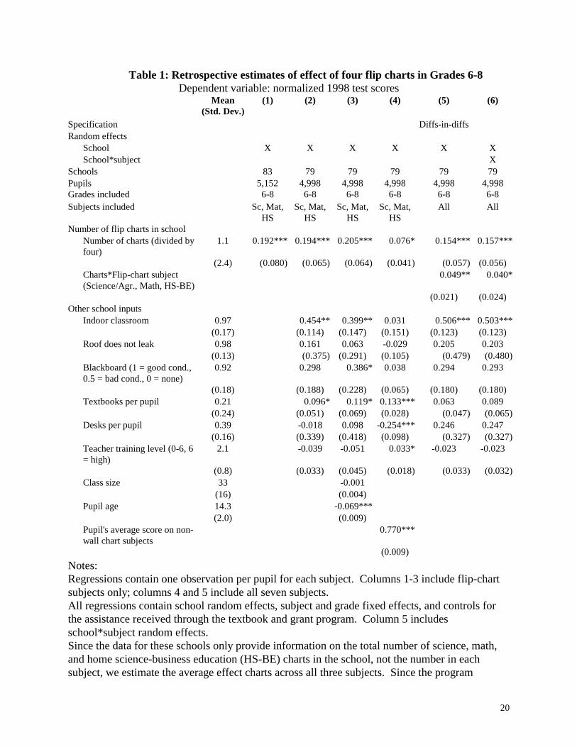
Table 1 presents results from regressions of test scores on flip charts and other

school inputs. In all regressions, data from multiple subjects and four grade-test

combinations (practice exam for grades 6-8 and KCPE for grade 8) are combined into a

single regression. Columns 1-4 estimate the effect of flip charts in the three flip chart

subjects. Columns 5 and 6 present results from a difference-in-differences specification

that compares the impact of flip charts on the relative performance of students in the three

flip chart and the four non-flip chart subjects. All regressions include subject and grade-

test fixed effects, and controls for whether the school was in a group that received

textbooks or grants through another program, (the omitted category is the comparison

group for that program). Thus, the coefficient on books per pupil reflects only variation

in textbooks due to other factors, primarily the number of books prior to the program.

Regressions also include school random effects to allow for within school correlation in

test scores for example, due to differences in headmaster quality.

The results in columns 1-3 suggest that adding flip charts raises test scores by

about 20 percent of a standard deviation in flip-chart subjects, an estimate which is

9

significant at the 5 percent level. Controlling for other school inputs makes little

difference to the estimates.

The estimators in columns 4-6 implicitly compare the relative performance of flip

charts in flip chart and non-flip chart subjects. The effect of flip charts is estimated by

comparing, across schools with and without flip charts, the difference between scores in

subjects where flip charts are used and scores in other subjects. The validity of this

approach is open to question. Some question whether it is possible to add and subtract

test scores in different subjects, given their ordinal, rather than cardinal nature (Krueger

and Whitmore, 2000). Aside from this issue, these estimators will only be valid if flip

charts have no effect on test scores in non-flip chart subjects, and if other factors

correlated with flip charts that could influence scores do so equally across all subjects.

Each of these assumptions is open to question. Flip charts could potentially either raise

or lower test scores in other subjects. They could raise test scores by improving pupils’

general interest in school, and thus attendance, or they could lower scores by diverting

pupils’ or teachers’ attention from non-flip chart subjects.6 Moreover, since different

tests were given in different subjects, an omitted variable correlated with flip charts, such

as headmaster characteristics, could potentially differentially affect test scores in different

subjects.

Column 4 controls for the performance of students in non-flip charts subjects; this

reduces the estimate to 7.6 percent, but this estimate remains significant. The

differences-in-differences estimates in columns 5 suggest that providing four flip charts

would raise test scores by 4.9 percent of a standard deviation in the three flip chart

10

subjects. Given that these regressions compare results across subjects, and that the

performance of students in a particular school in a particular subject may be correlated

due to teacher ability, column 6 allows for random effects at the level of interaction

between schools and subjects. This reduces the point estimate to 4 percent, and

considerably reduces the significance level given the small sample size. The differences-

in-differences regressions also suggest that flip charts raise test scores by 15-16 percent in

non-flip chart subjects, suggesting either that flip charts have a positive effect in non-flip

chart subjects or that the direct estimators are inflated by an omitted variable bias

problem that controlling for other school inputs does not alleviate.7

The retrospective analysis makes flip charts look cost effective compared to

textbooks. The per-pupil cost of providing four charts is only 10 percent of the cost of

providing a textbook for every pupil in each of the three subjects,8 but the retrospective

estimates suggest that the flip chart effect is about 50 percent larger than the effect of

providing textbooks for each pupil in three subjects (from column 2, comparing 0.194 --

the effect of four charts -- with 0.125). Since flip charts are much less expensive, the

relative cost-effectiveness of these two interventions is much higher, with flip charts

being about 15 times more cost-effective than textbooks, in terms of dollars per average

6 Note, however, that in the upper grades, the school day is divided into separate periods with differentteachers for different subjects.7 A caveat to the retrospective analysis is that the significance of some of the results is caused by theinclusion of one school with well above average test scores and 15 charts (compared with an average of 1.1per school). Although we have no reason to doubt this data, treating the school has having only 5 chartsreduces the estimates in column 2 to 18 percent with a standard error of 16 percent. The differences-in-differences estimate in column 4 remains significant and increases slightly in magnitude, however.8 Wall charts cost about US$20 each, so four would cost $80. Textbooks in Kenya cost approximately$3.33; it would therefore cost about $800 to provide one textbook per pupil in each of three subjects to the80 students in grades 6-8 at the average-sized school in the sample. These cost figures are from 1997 andare converted to US$ at the then current exchange rate of 60Ksh/$.

11

test score gain. Even though the differences-in-differences estimate is much smaller than

the direct estimate, it still suggests that flip charts are 3-4 times as cost-effective in raising

average test scores as textbooks. As discussed below, a prospective analysis does not

support this conclusion.

III. Prospective Analysis

Internationaal Christelijk Steunfonds (ICS), a Dutch non-governmental

organization, distributed flip charts to selected schools in Busia and Teso in 1997. One

hundred and seventy-eight schools were potentially eligible. Schools that ICS had

previously assisted through the textbook and grant program or through other programs

were ineligible, as were a smaller number of relatively well-off schools. Since ICS began

assisting schools that were relatively poor, those participating in the textbook/grant study

tended to be slightly worse performers than those in the flip chart study, and since the

best off schools were excluded, those in the flip chart study had roughly similar mean

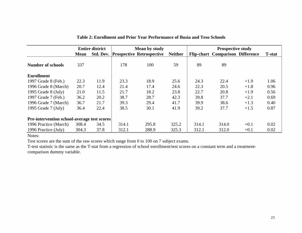
scores as the district as a whole.9 Table 2 shows that the average pre-intervention

characteristics of these 178 schools were nonetheless fairly close to those of the district as

a whole. The assignment of the 178 schools into flip chart and comparison groups was

done as follows; the schools were sorted alphabetically, first by geographic district, then

by geographic division, and then by school name. Then every other school on that list

9 If flip charts were more helpful for weaker students, part of the difference explanation for larger estimatedeffect for the retrospective could be that these schools had lower average 1996 test scores. Interactionregressions in both the retrospective and the prospective sample found no evidence that the effect of flip-charts was greater for schools with low initial test scores. The point estimates for the interaction coefficientssuggested that the effect of flip charts would be between –0.4 and 0.2 percent higher in the retrospectivesample; these point estimates were statistically insignificant.

12

was placed in the flip chart group. The two types of schools will henceforth be referred to

as flip-chart schools and comparison schools, respectively. The flip chart program was

announced in January 1997, after the start of the 1997 school year (in Kenya the school

year runs from January to November), and the charts were distributed in early February

1997. Each school received two sets of science charts (including a teacher’s guide), one

set of charts in math, one set in health, and a wall map.

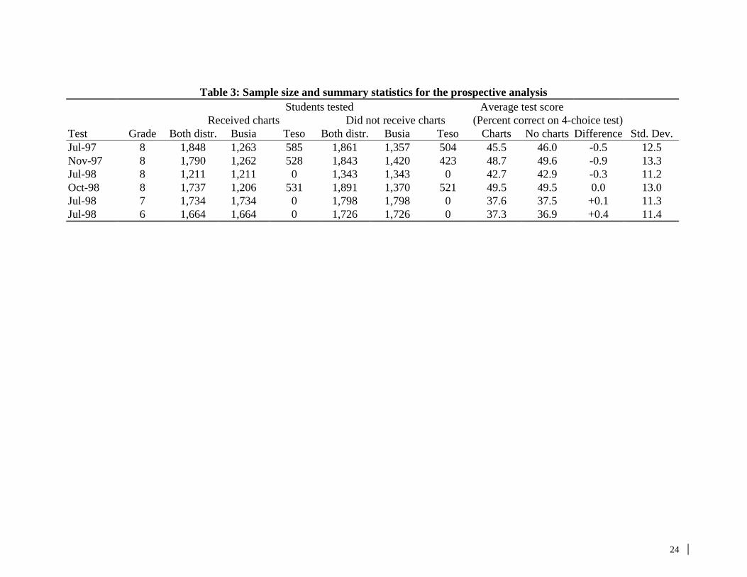
Table 3 contains the average raw scores out of 100 for each test and grade for the

flip chart and comparison schools in the prospective study. The most straightforward

method of evaluating the effect of the randomized distribution of flip charts is to compare

the post-intervention (1997 and 1998) scores in the 89 flip chart schools with the scores

in the 89 comparison schools. The last four columns of Table 3 provide average test

scores across all seven subjects for the flip chart and comparison schools for each test and

grade combination. The flip chart schools scored equal to or slightly below the

comparison schools on the grade 8 exams and slightly above the comparison schools in

grades 6 and 7 on the July 1998 exam. In all cases, the differences are much less than 10

percent of a standard deviation of the distribution for the comparison group.

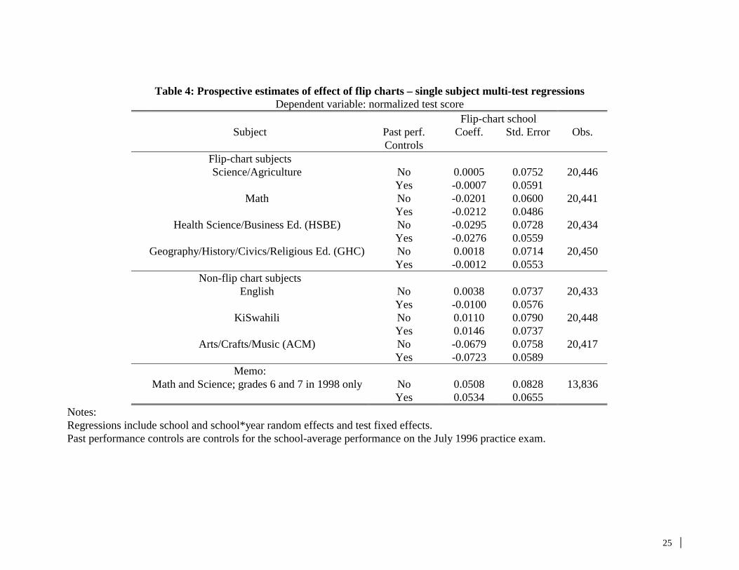
Table 4 presents random effects regression estimates of the difference in test

scores between flip chart and comparison schools for each subject. Data from all tests are

pooled to construct these estimators. School random effects are included to allow for

correlation in the error term among students within a school, and these school random

effects are allowed to vary by year. Results are presented with and without controls for

pre-intervention (1996) school-average test scores. Controlling for pre-intervention test

scores reduces the size of the school random effect, improving the efficiency of

13

estimation. For science-agriculture, the subject for which two sets of flip charts and a

teacher guide were given, test scores for the flip chart and comparison schools were

almost identical; the same is true for Geography/History/Civics/Religion. For math and

Home Science/Business Education, scores in flip chart schools were 2-3 percent of a

standard deviation below those of comparison schools. None of these differences is

statistically significant. Even if we limit the analysis to the subject-grade combinations in

which charts appear most promising, namely Math and Science in grades 6 and 7, a

procedure that is obviously open to criticisms of data mining, we still do not obtain a t-

statistic greater than one. In summary, there is little evidence in Table 4 that suggests flip

charts had a positive impact on test scores.

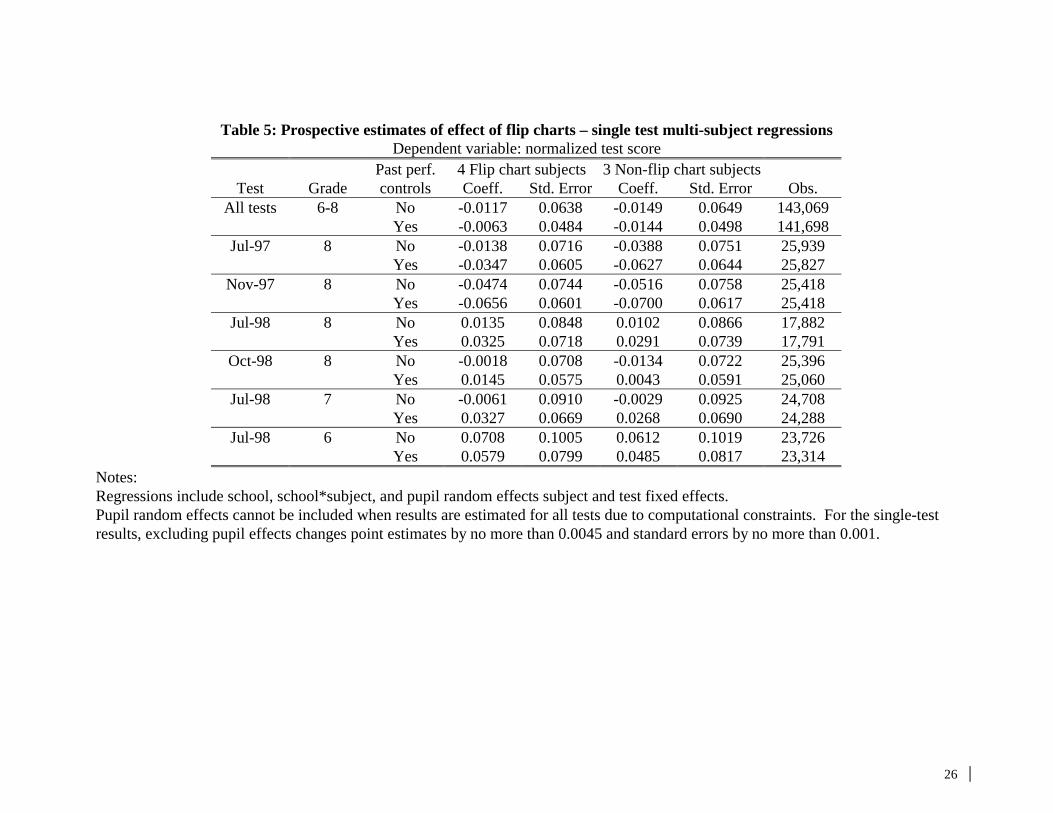
Tables 5 and 6 present estimates that pool across subjects. In Table 5, the

estimate of the difference between flip chart and comparison schools is allowed to vary

for the four flip-chart subjects and the three non-flip chart subjects. This estimation

includes random effects for school, school-subject combinations, and pupils.10

Controlling for pre-intervention school-average scores and combining all tests, test scores

in schools that received flip charts are estimated to be 0.6 and 1.4 percent of a standard

deviation lower in flip chart and non flip-chart subjects, respectively, with standard errors

of roughly 5 percent of a standard deviation. Again controlling for pre-intervention

school-average scores, scores are 3-7 percent of a standard deviation lower in flip-chart

schools in both groups of subjects in 1997, while they are 2-6 percent of a standard

10 Due to computational constraints, pupil random effects could not be included in the regressions whichinclude all subject-grade-test combinations. Despite the large size of the pupil random effects, the resultsfor the single-test, multi-subject regressions change very little when pupil random effects are omitted. Flipchart effects change by no more than 0.45 percent of a standard deviation, and standard errors increase by

14

deviation higher on the 1998 practice exam. None of these differences are close to being

statistically significant (none has a t-statistic over 0.75), nor is the slight improvement

from 1997 to 1998 statistically significant in regressions that estimate separate flip-chart

effects for each year for 8th graders (not shown).

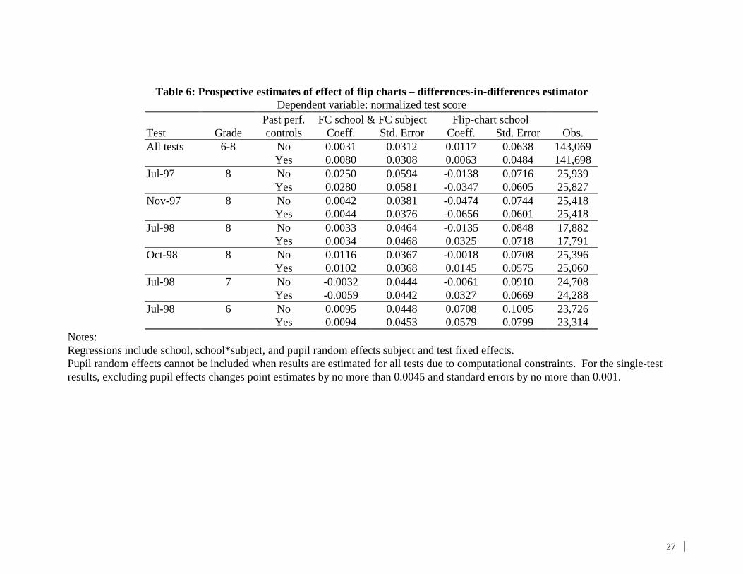
The results in Table 5 suggest that the overall performance of a school can vary

from year to year across subjects. This variation in the cross-subject school effect adds

noise to the estimated difference between test scores in flip chart and non flip chart

schools. An alternative approach is to assume that flip charts do not affect performance

in non flip-chart subjects and estimate the effect of flip charts by comparing the relative

performance of flip-chart schools in flip chart and non flip chart subjects with the

analogous relative performance in the comparison schools. Under the assumption that

flip charts do not affect non-flip chart subjects, we can improve the efficiency of

estimation by using the non-flip chart subjects to better control for school effects. Table

6 presents estimates of the difference in the flip chart-comparison school performance

differential between flip chart and non flip-chart subjects. Across all subjects and test-

grade combinations and controlling for past performance, the effect of flip charts is

estimated to be 0.8 percent of a standard deviation. The standard error of the differences-

in-differences estimator is lower (3.1 percent of a standard deviation), but the estimated

effect of flip charts is still far from significant.

Across all the different estimators in the prospective study, the effect of flip charts

appears to be essentially zero. There is no evidence that this is because flip charts were

0.1 percent of a standard deviation for 8th grade and decrease by 0.04 percent for 6th and 7th grade, whenpupil random effects are omitted.

15

not used. We interviewed 82 grade 7 and 8 teachers in flip-chart subjects at 21 of the

schools that received flip charts. Ninety-eight percent of the teachers were aware that

their school had been given flip charts, and 91 percent claimed to have used the flip

charts. In no cases had the flip charts been lost or stolen. Ninety-two percent of teachers

claimed they found the charts helpful, and they reported that the average chart had been

used in each class on 10-20 percent of school days in the current year (1998). Given that

the charts were shared between grades 6-8 at least, this represents reasonably high

utilization of the charts. One caveat is that although teachers were surveyed in private

and told that their answers would be kept confidential and would not affect future aid to

their school, the teachers may have nonetheless felt an incentive to bias their usage

estimates upward. Yet over ninety percent of the teachers gave specific answers to

questions that required some experience using the charts (e.g., which charts did they find

most and least helpful, and why), which suggests that the charts had at least been used.

The incentives faced by schools in Busia may have led them to use the charts for

students in upper grades, who would soon take the KCPE exam on which schools are

judged. The flip chart use survey revealed that charts were used an average of 13 days

per 75-day term in grade 8 compared to 7 days each in grades 6 and 7. One potential

hypothesis for the low estimated effect of flip charts is that the charts would have been

more useful in lower grades. Thirty percent of grade 7 and 8 teachers reported that the

charts helped the worst students the most, while only three percent reported that they

helped the best students most. The fact that the estimated effect of the flip charts was

highest for grade 6 students is at least consistent with the charts being more appropriate

for those students. However, neither the estimated effect for grade 6 nor the difference in

16

estimated effect between grade 6 and the higher grades is statistically significant. We

also used quantile regressions to test whether flip charts had a greater impact for lower-

ability students and found that the coefficients from the quantile regressions did not differ

with those from mean regressions by more than one percent of a standard deviation and

remained insignificant.

Note that even the lowest retrospective estimate implies that the program should

have raised scores by four percent of a standard deviation, while the levels retrospective

estimator suggests that it should have raised scores by 20 percent of a standard deviation.

The latter possibility is rejected by the prospective study, although the former is within a

95-percent confidence interval.

IV. Missing data and potential biases

The results of both the prospective and retrospective evaluations could be biased

if the probability of our observing the test score of pupils of different ability were affected

differentially by the flip charts. In particular, both estimates could be biased downward if

flip charts induced more low-ability students to take the exams. We do not have data to

check this for our retrospective estimates, but in the prospective study, absenteeism rates

for each exam were very similar in the treatment and control schools. Probit regressions

(not shown here) reveal that the differences in absenteeism are not significant, and the

magnitude of the differences is small enough that even if it were the worst students that

missed the tests, the effect on the average result would be small.

17

More specifically, absenteeism rates for flip chart and comparison schools in 1997

were 2.2 and 2.4 percent for the practice and 1.0 and 1.2 percent for the KCPE exam.

Absenteeism rates for flip-chart and comparison schools for grade 8 in 1998 were 6.3 and

3.8 percent for the practice exam and 3.5 and 3.1 percent for the KCPE exam;

absenteeism for the practice exam was 10.8 and 10.8 for grade 6 and 9.4 and 6.9 for grade

7. The largest differences were for the 1998 grade 7 and 8 practice exams, where

absenteeism for flip-chart schools was 2.5 percentage points higher. If the marginal

student was one standard deviation below the mean on each individual test, this

difference in absenteeism would lead to an overestimate of the relative performance of

the treatment schools by 2.5 percent of a standard deviation on these two tests; the

differences for the other exams would be trivial. The assumption that non-takers would

score one standard deviation below the mean is probably extreme given that in 1998, 8th

graders who did not take the KCPE scored only 0.1 standard deviations on the practice

exam below those who did. It is therefore unlikely that absenteeism is responsible for the

results.

In addition, due to illegible or lost score recording sheets or non-administration of

the exam, 6, 14, 15, 14, 1, and 2 schools were missing scores for the 1997 grade 8

practice and KCPE, 1998 grades 6-8 practice, and 1998 grade 8 KCPE, respectively.

Roughly half of the school missing data were comparison schools (4, 8, 6, 8, 1, and 2,

respectively). The missing schools were roughly average performers on the 1996 tests, so

their omission should not systematically affect the results, and any effect should be

mitigated by controlling for 1996 test performance. For example, the difference between

the average raw 1996 score for the schools with data and for all the schools was +0.45

18

and +0.25 points (out of 100 points) for the flip-chart and comparison groups in 1997,

respectively. In terms of standard deviations, this corresponds to average individual test

differences of 0.6 and 0.4 percent of a standard deviation, respectively. In 1996,

excluding the schools with missing 1997 data would therefore have lead to an

overestimate of the relative scores of the flip-chart schools on the average individual test

by 0.2 percent of a standard deviation. Assuming that any effect on the 1997 and 1998

results would be roughly of this magnitude, there is little reason to think that the inclusion

of the missing schools would materially affect the results.

Conclusion

The analysis in this paper leads to two conclusions. First, prospective estimates of

the impact of flip charts on children’s performance on academic tests in Kenya show no

impact at all of these charts on learning.11

Second, the analysis suggests that the most obvious retrospective regressions

would have greatly overestimated the effect of a program providing flip charts on a large

scale. More subtle retrospective analyses that compare test scores across subjects appear

to reduce the bias significantly in the case of the flip chart intervention, which focused on

particular subjects, but such techniques are not applicable for other inputs, such as school

buildings or smaller pupil-teacher ratios, which affect all subjects, and could easily go

astray in other contexts, given the ordinal nature of test score data.

19

There are two possible interpretations of the difference between the retrospective

and prospective results. The schools in the retrospective sample that had flip charts may

have differed from others in unobserved ways that raised their test scores independently

of whether they had flip charts. Alternatively, the schools with flip charts may have

differed from others in ways that would not have affected their test scores in the absence

of flip charts, but which made flip charts particularly useful. Under either hypothesis,

retrospective estimates would be a poor guide to the effects of a large-scale program to

provide flip charts, but under the second hypothesis, they would be an appropriate

measure of the effect of flip charts on those schools that choose to purchase them. The

fact that test scores were higher in schools with flip charts, even in subjects where wall

charts were not applicable, tends to support the first hypothesis, that schools with charts

had higher test scores for reasons other than a causal effect of flip charts.

The omitted-variable bias in the retrospective estimates seems to lead to

overestimation of treatment effects. The direction of bias makes sense in a developing

country context, where compensatory programs are rare. If this result proves robust, it

suggests that Hanushek’s (1995) pessimistic conclusions about the effects of school

inputs in developing countries based on retrospective studies may be strengthened, rather

than weakened, by prospective studies.

11 It is worth noting, however, that given that flip charts are very cheap, and that our standard errors are nottiny, we cannot rule out the possibility that flip charts are a good investment.

20

Table 1: Retrospective estimates of effect of four flip charts in Grades 6-8Dependent variable: normalized 1998 test scores

Mean(Std. Dev.)

(1) (2) (3) (4) (5) (6)

Specification Diffs-in-diffsRandom effects

School X X X X X XSchool*subject X

Schools 83 79 79 79 79 79Pupils 5,152 4,998 4,998 4,998 4,998 4,998Grades included 6-8 6-8 6-8 6-8 6-8 6-8Subjects included Sc, Mat,

HSSc, Mat,

HSSc, Mat,

HSSc, Mat,

HSAll All

Number of flip charts in schoolNumber of charts (divided byfour)

1.1 0.192*** 0.194*** 0.205*** 0.076* 0.154*** 0.157***

(2.4) (0.080) (0.065) (0.064) (0.041) (0.057) (0.056)Charts*Flip-chart subject(Science/Agr., Math, HS-BE)

0.049** 0.040*

(0.021) (0.024)Other school inputs

Indoor classroom 0.97 0.454** 0.399** 0.031 0.506*** 0.503***(0.17) (0.114) (0.147) (0.151) (0.123) (0.123)

Roof does not leak 0.98 0.161 0.063 -0.029 0.205 0.203(0.13) (0.375) (0.291) (0.105) (0.479) (0.480)

Blackboard (1 = good cond.,0.5 = bad cond., 0 = none)

0.92 0.298 0.386* 0.038 0.294 0.293

(0.18) (0.188) (0.228) (0.065) (0.180) (0.180)Textbooks per pupil 0.21 0.096* 0.119* 0.133*** 0.063 0.089

(0.24) (0.051) (0.069) (0.028) (0.047) (0.065)Desks per pupil 0.39 -0.018 0.098 -0.254*** 0.246 0.247

(0.16) (0.339) (0.418) (0.098) (0.327) (0.327)Teacher training level (0-6, 6= high)

2.1 -0.039 -0.051 0.033* -0.023 -0.023

(0.8) (0.033) (0.045) (0.018) (0.033) (0.032)Class size 33 -0.001

(16) (0.004)Pupil age 14.3 -0.069***

(2.0) (0.009)Pupil's average score on non-wall chart subjects

0.770***

(0.009)

Notes:Regressions contain one observation per pupil for each subject. Columns 1-3 include flip-chartsubjects only; columns 4 and 5 include all seven subjects.All regressions contain school random effects, subject and grade fixed effects, and controls forthe assistance received through the textbook and grant program. Column 5 includesschool*subject random effects.Since the data for these schools only provide information on the total number of science, math,and home science-business education (HS-BE) charts in the school, not the number in eachsubject, we estimate the average effect charts across all three subjects. Since the program

21

evaluated in the prospective study distributed four flip charts (2 Science, 1 Math, 1 HS-BE), wedivide the number of charts variable by four to generate coefficients that are comparable with theretrospective analysis.Standard errors are heteroskedasticity robust.Statistical significance at the 10, 5, and 1 percent level is indicated by 1, 2, and 3 asterisks,respectively.

23

Table 2: Enrollment and Prior Year Performance of Busia and Teso Schools

Entire district Mean by study Prospective studyMean Std. Dev. Prospective Retrospective Neither Flip-chart Comparison Difference T-stat

Number of schools 337 178 100 59 89 89

Enrollment1997 Grade 8 (Feb.) 22.3 11.9 23.3 18.9 25.6 24.3 22.4 +1.9 1.061996 Grade 8 (March) 20.7 12.4 21.4 17.4 24.6 22.3 20.5 +1.8 0.961995 Grade 8 (July) 21.0 11.5 21.7 18.2 23.8 22.7 20.8 +1.9 0.561997 Grade 7 (Feb.) 36.2 20.2 38.7 28.7 42.3 39.8 37.7 +2.1 0.691996 Grade 7 (March) 36.7 21.7 39.3 29.4 41.7 39.9 38.6 +1.3 0.401995 Grade 7 (July) 36.4 22.4 38.5 30.1 41.9 39.2 37.7 +1.5 0.87

Pre-intervention school-average test scores1996 Practice (March) 308.4 34.5 314.1 295.8 325.2 314.1 314.0 +0.1 0.021996 Practice (July) 304.3 37.8 312.1 288.9 325.3 312.1 312.0 +0.1 0.02Notes:Test scores are the sum of the raw scores which range from 0 to 100 on 7 subject exams.T-test statistic is the same as the T-stat from a regression of school enrollment/test scores on a constant term and a treatment-comparison dummy variable.

24

Table 3: Sample size and summary statistics for the prospective analysisStudents tested Average test score

Received charts Did not receive charts (Percent correct on 4-choice test)Test Grade Both distr. Busia Teso Both distr. Busia Teso Charts No charts Difference Std. Dev.Jul-97 8 1,848 1,263 585 1,861 1,357 504 45.5 46.0 -0.5 12.5Nov-97 8 1,790 1,262 528 1,843 1,420 423 48.7 49.6 -0.9 13.3Jul-98 8 1,211 1,211 0 1,343 1,343 0 42.7 42.9 -0.3 11.2Oct-98 8 1,737 1,206 531 1,891 1,370 521 49.5 49.5 0.0 13.0Jul-98 7 1,734 1,734 0 1,798 1,798 0 37.6 37.5 +0.1 11.3Jul-98 6 1,664 1,664 0 1,726 1,726 0 37.3 36.9 +0.4 11.4

25

Table 4: Prospective estimates of effect of flip charts – single subject multi-test regressionsDependent variable: normalized test score

Flip-chart schoolSubject Past perf.

ControlsCoeff. Std. Error Obs.

Flip-chart subjectsScience/Agriculture No 0.0005 0.0752 20,446

Yes -0.0007 0.0591Math No -0.0201 0.0600 20,441

Yes -0.0212 0.0486Health Science/Business Ed. (HSBE) No -0.0295 0.0728 20,434

Yes -0.0276 0.0559Geography/History/Civics/Religious Ed. (GHC) No 0.0018 0.0714 20,450

Yes -0.0012 0.0553Non-flip chart subjects

English No 0.0038 0.0737 20,433Yes -0.0100 0.0576

KiSwahili No 0.0110 0.0790 20,448Yes 0.0146 0.0737

Arts/Crafts/Music (ACM) No -0.0679 0.0758 20,417Yes -0.0723 0.0589

Memo:Math and Science; grades 6 and 7 in 1998 only No 0.0508 0.0828 13,836

Yes 0.0534 0.0655Notes:Regressions include school and school*year random effects and test fixed effects.Past performance controls are controls for the school-average performance on the July 1996 practice exam.

26

Table 5: Prospective estimates of effect of flip charts – single test multi-subject regressionsDependent variable: normalized test score

Past perf. 4 Flip chart subjects 3 Non-flip chart subjectsTest Grade controls Coeff. Std. Error Coeff. Std. Error Obs.

All tests 6-8 No -0.0117 0.0638 -0.0149 0.0649 143,069Yes -0.0063 0.0484 -0.0144 0.0498 141,698

Jul-97 8 No -0.0138 0.0716 -0.0388 0.0751 25,939Yes -0.0347 0.0605 -0.0627 0.0644 25,827

Nov-97 8 No -0.0474 0.0744 -0.0516 0.0758 25,418Yes -0.0656 0.0601 -0.0700 0.0617 25,418

Jul-98 8 No 0.0135 0.0848 0.0102 0.0866 17,882Yes 0.0325 0.0718 0.0291 0.0739 17,791

Oct-98 8 No -0.0018 0.0708 -0.0134 0.0722 25,396Yes 0.0145 0.0575 0.0043 0.0591 25,060

Jul-98 7 No -0.0061 0.0910 -0.0029 0.0925 24,708Yes 0.0327 0.0669 0.0268 0.0690 24,288

Jul-98 6 No 0.0708 0.1005 0.0612 0.1019 23,726Yes 0.0579 0.0799 0.0485 0.0817 23,314

Notes:Regressions include school, school*subject, and pupil random effects subject and test fixed effects.Pupil random effects cannot be included when results are estimated for all tests due to computational constraints. For the single-testresults, excluding pupil effects changes point estimates by no more than 0.0045 and standard errors by no more than 0.001.

27

Table 6: Prospective estimates of effect of flip charts – differences-in-differences estimatorDependent variable: normalized test score

Past perf. FC school & FC subject Flip-chart schoolTest Grade controls Coeff. Std. Error Coeff. Std. Error Obs.All tests 6-8 No 0.0031 0.0312 0.0117 0.0638 143,069

Yes 0.0080 0.0308 0.0063 0.0484 141,698Jul-97 8 No 0.0250 0.0594 -0.0138 0.0716 25,939

Yes 0.0280 0.0581 -0.0347 0.0605 25,827Nov-97 8 No 0.0042 0.0381 -0.0474 0.0744 25,418

Yes 0.0044 0.0376 -0.0656 0.0601 25,418Jul-98 8 No 0.0033 0.0464 -0.0135 0.0848 17,882

Yes 0.0034 0.0468 0.0325 0.0718 17,791Oct-98 8 No 0.0116 0.0367 -0.0018 0.0708 25,396

Yes 0.0102 0.0368 0.0145 0.0575 25,060Jul-98 7 No -0.0032 0.0444 -0.0061 0.0910 24,708

Yes -0.0059 0.0442 0.0327 0.0669 24,288Jul-98 6 No 0.0095 0.0448 0.0708 0.1005 23,726

Yes 0.0094 0.0453 0.0579 0.0799 23,314Notes:Regressions include school, school*subject, and pupil random effects subject and test fixed effects.Pupil random effects cannot be included when results are estimated for all tests due to computational constraints. For the single-testresults, excluding pupil effects changes point estimates by no more than 0.0045 and standard errors by no more than 0.001.

29

References

Davis, O. L., Jr. 1968. “Effectiveness of Using Graphic Illustrations with Social StudiesTextual Materials. Final Report.” Kent State University, Ohio..

Dunn, Rita, et al. 1989. Learning Styles Inventory. Reston, VA.

Dwyer, Francis M., Jr. 1970. “Exploratory Studies in the Effectiveness of VisualIllustrations.” AV Communication Review, 235-49.

Dwyer, Francis M., Jr. 1976. “The Effect of IQ Level on the Instructional Effectivenessof Black-and-White and Color Illustrations.” AV Communication Review, 49-62.

Glewwe, Paul, Michael Kremer and Sylvie Moulin. 2000. “Textbooks and Test Scores:Evidence from a Prospective Evaluation in Kenya.” Policy Research Group. The WorldBank.

Hanushek, Eric. 1986. “The Economics of Schooling: Production and Efficiency inPublic Schools.” Journal of Economic Literature, September, pp. 1141-77.

Hanushek, Eric. 1995. “Interpreting Recent Research on Schooling in DevelopingCountries.” World Bank Research Observer, August, pp. 227-46.

Hanushek, Eric and Rivlin. 1997. “Understanding the 20th Century Growth in U.S.School Spending.” Journal of Human Resources, Winter, pp. 35-68.

Harbison, Ralph W. and Eric Hanushek. 1992. Educational Performance of the Poor,Lessons From Rural Northeast Brazil. World Bank, Washington D.C.

Hedges, Laine, and Greenwald. 1994. “Does Money Matter? A Meta-Analysis ofStudies of the Effects of Differential School Inputs on Student Outcomes.” EducationalResearcher, April, pp. 5-14.

Holliday, William G. 1973. “A Study of the Effects of Verbal and Adjunct PictorialInformation in Science Instruction.” Mimeo, Ohio State University.

Holliday, William G. 1976. “Teaching Verbal Chains Using Flow Diagrams and Text.”AV Communication Review, 1976, 63-78.

Holliday, William and Garth Benson. 1991. “Enhancing Learning Using QuestionsAdjunct to Science Charts.” Journal of Research in Science Teaching, January, 97-108.

Kiesling, Herbert J. 1967. “Measuring Local Government Service: A Study of SchoolDistricts in New York State.” Review of Economic Studies, August, pp. 356-67.

30

Kremer, Michael, Sylvie Moulin, Robert Namunyu and David Myatt. 1997. “TheQuantity-Quality Tradeoff in Education: Evidence from a Prospective Evaluation inKenya”. Unpublished.

Krueger, Alan B. and Diane M. Whitmore. 2000. “The Effect of Attending a SmallClass in the Early Grades on College-Test Taking and Middle School Results: Evidencefrom Project STAR.” NBER Working Paper No. 7656.

LaLonde, Robert J. 1986. “Evaluating the Econometric Evaluations of TrainingPrograms with Experimental Data.” American Economic Review, 76(4), September,604-20.

Levin, Joel R., et al. 1976. “Pictures, Repetition, and Young Children’s Oral ProseLearning.” AV Communication Review, 24 (4), Winter, 367-380.

Lookatch, Richard P. 1995. “The Strange but True Story of Multimedia and the Type IError.” Technos, Summer, 10-13.

Lowe, Richard. 1989. “Scientific Diagrams: How Well Can Students Read Them?What Research Says to the Science and Mathematics Teacher.” Mimeo, CurtinUniversity of Technology.

McAlister, Brian. 1991. “Effects of Analogical vs. Schematic Illustrations on InitialLearning and Retention of Technical Material by 8th Grade Students.” Paper presented atthe American Vocational Association Convention, Los Angeles, CA.

Samuels, S.J. 1970. “Effects of Pictures on Learning-To-Read, Comprehension, andAttitude.” Review of Educational Research, Vol. 16, 397-407.

Shepard, Roger. 1967. “Recognition Memory for Words, Sentences, and Pictures.”Journal of Verbal Learning and Verbal Behavior, Vol. 6.

Wallace, James. 1995. “Accommodating Elementary Students’ Learning Styles.”Reading Improvement, Spring, 38-41.