Embed Size (px)
Citation preview

Retrospective Analysis of Preseason Run Forecast Models for Warm Springs stock
Spring Chinook Salmon in the Deschutes River, Oregon
David Hand and Steve Haeseker
USFWS-Columbia River Fisheries Program Office
November 2011
Summary
A retrospective analysis of run forecast models for Warm Spring River wild and Warm
Springs NFH hatchery spring Chinook salmon was performed based on the methods of
Haeseker et al. 2008. The two models that are currently used for run forecasting, the
standard linear regression model and cohort model (Lovtang et al. 2011), were re-run on
an annual basis starting with return year 1990 using only the data that would have been
available to managers at the time. In addition, several alternative forecast models that are
used throughout the Pacific Northwest were evaluated for comparison to the traditional
forecast models. Performance of each model was evaluated using a variety of metrics
that quantify a forecast model’s accuracy.
Based on the historical data analyzed, several actions could be taken to improve the
forecasting of spring Chinook salmon returns to the Deschutes basin. Recommendations
for wild fish forecasts are:
Use a 10 year rolling dataset for the standard regression model.
Use the percent-by-age model, with 10 year rolling datasets, to supplement
the traditional forecast models. The percent-by-age model could replace
the cohort model in the run prediction reports.
Add a zone (red, yellow, green) descriptor to the point estimates in run
prediction reports. Forecasts in the red zone would indicate a high
probability of not meeting wild fish escapement goals, in the yellow zone
a moderate probability of not meeting wild fish escapement goals, and in
the green zone a low probability of not meeting minimum wild fish
escapement goals. Statistics, including confidence intervals and
evaluation of past model performance should continue to be included in
run prediction reports.
Continue to evaluate forecast model performance on an annual basis.
Recommendations for Warm Springs NFH hatchery fish forecasts are:
Use natural log transformed data for regression model forecasts.
Use the percent-by-age model to supplement the traditional run forecast
models. The percent-by-age model could replace the cohort model in the
run prediction reports.
Continue to evaluate forecast model performance on an annual basis.

Introduction
Run forecasts for spring Chinook salmon in the Deschutes basin are based on sibling
models in which returns of younger aged fish are used to predict returns of older age fish
in subsequent years. Forecast accuracy has important implications for management of
salmon in the basin, yet the forecast confidence intervals that are generated using sibling
models are often quite large, complicating management decisions. Looking back at how
the run forecasts models have actually performed in comparison to returns may provide
managers with additional perspective regarding run size estimates. In addition, alternative
forecast models that are used throughout the Pacific Northwest may improve forecast
performance in comparison to the traditional forecast methods used in the Deschutes
Basin.
Methods
Run reconstruction data of wild Warm Springs River spring Chinook salmon for brood
years (BY) 1975 to 2006, and Warm Springs NFH hatchery spring Chinook salmon for
BY 1978 to 2006 were used to estimate the number of age 3, age 4, and age 5 fish that
returned to the mouth of the Deschutes River for a given brood year. Run reconstruction
methods and data can be found in the annual run forecast reports (Lovtang et al. 2011).
Run forecasts for the Deschutes River are made for adult sized fish only, that is age 4 and
age 5 spring Chinook salmon returns in a given year. For the retrospective analysis, run
forecasts were made for wild adult returns starting with return year 1990, which would be
comprised of age 4 returns from BY 1986 and age 5 returns from BY 1985. Return year
1990 was chosen as the starting point so that each wild forecast model would have 10
brood years (BY 1975 to BY 1984) worth of data to start with. For the hatchery forecast
models, forecasts were made starting with return year 1993, again so that each forecast
model would have 10 brood years (BY 1978 to 1987) of data.
For each model type analyzed, retrospective forecasts were made for total adult (age 4
and age 5) returns for return years 1990 to 2010 for wild fish and return years 1993 to
2010 for hatchery fish. Each forecast was made using only the data that would have been
available at the time. For example, the 1990 adult return of wild fish was forecasted
using the standard linear regression model of age 3 to age 4, and age 4 to age 5 data
through return year 1989. For the 1991 forecast, regressions were run again but this time
using data through return year 1990, and so on. A total of 21 forecasts (return years 1990
to 2010) were made for wild fish and 18 forecasts (return years 1993 to 2010) for
hatchery fish using each model type.
The performance of each model was then analyzed using methods described in Haeseker
et al. 2008. Each retrospective forecast was compared to the observed return in each
year. Performance of each model was then evaluated using four performance measures:
the mean raw error, mean absolute error, mean percent error, and root mean square error
(RMSE) of the forecasts. Raw error is defined as the forecasted return minus the actual
return. Negative raw error values indicate over-forecasts, and positive values indicate
under-forecasts. The mean raw error, which is the raw error averaged over the number of
years forecasted, is a measure of the overall bias of the forecast. Years of over-forecast
can be offset by years of under-forecast, which would result in a mean raw error value
close to zero. To get an idea of the magnitude of forecast error, regardless of sign, the
mean absolute error was also calculated. Mean percent error was calculated as the raw
error divided by the actual return. The RMSE was calculated according to methods
described in Haeseker et al. 2008, and provides a measure of the forecast error variance.
Models with the lowest RMSE would produce the narrowest (best) confidence intervals.
Models were then ranked from best to worst for each performance measure.
In the Deschutes River basin, management of spring Chinook salmon is often based on
the number of wild fish expected to return to the Warm Springs River. The Confederated
Tribes of the Warm Springs Reservation of Oregon’s minimum escapement goal for wild
fish upstream of Warm Springs NFH is 1,000 adults. If less than 1,000 adults are
forecasted, no wild fish are incorporated into the Warm Springs NFH broodstock
(CTWSRO and USFWS 2007). In addition, if less than 1,000 wild adults are forecasted,
harvest restrictions are often imposed on the sport or Tribal fisheries in the Deschutes
River. To assess each forecast model’s management utility for wild fish management,
forecasts and actual returns of less than 1,000 adults were analyzed. The number of times
a model correctly and incorrectly forecasted less than 1,000 returning adults was
summarized. Plots of forecasted return and actual return were also used to analyze a
model’s tendency to over-forecast or under-forecast runs above or below the 1,000 fish
threshold.
A similar assessment was made for hatchery fish forecast models based on adult return
needs for hatchery production at Warm Springs NFH. Current hatchery production goals
require a broodstock of 630 adult fish (CTWSRO and USFWS 2007). The harvest rate
of Warm Springs NFH stock adults in the sport and Tribal fishery at Sherars Falls has
averaged around 30% (unpublished data). A return of 1,000 Warm Springs NFH
hatchery adults was used as the critical management point, with the assumption that a
30% harvest rate would result in 700 adults returning to Warm Springs NFH, sufficient
for broodstock needs.
In the Deschutes Basin, several run forecasting models have been utilized over the years.
In recent years, run forecasts have been based on a standard regression model and a
cohort model (Lovtang et al. 2011). These two “standard” models were analyzed along
with a variety of alternative models that have been used either in the Deschutes basin or
for other salmon runs in the Pacific Northwest. The forecast models used in this
retrospective analysis were:
1) The “standard” linear regression model as described in Lovtang et al.
2011, to predict the age 4 and age 5 returns. The standard regression
model assumes a linear relationship between two sibling groups. For
the Deschutes River forecasts, linear regression of age 3 (x) to predict
age 4 returns (y) and age 4 (x) to predict age 5 returns (y) were

calculated. The forecasted age 4 and age 5 returns were then added to
arrive at a total adult return forecast. For example, the formula for
predicting age 4 returns in year t is: age 4year t =a+(b*age 3year t-1),
where a and b are estimated parameters from the linear regression.
2) A natural log (LN) transformed regression model as described in Peterman
1982 and Haeseker et al. 2008. This model is similar to the standard
regression model, however loge transformed data is used to construct
the regression and then the result is back-transformed into an
arithmetic scale. The formula for predicting age 4 returns in year t is:
loge(age 4year t)=a+b*loge(age 3year t-1)+E, where E is an error term used
to account for bias in back-transforming lognormal distributions (see
Heaseker et al. 2008 for discussion).
3) The “standard” cohort age at return ratio method as described in Lovtang
et al. 2011. This method uses the mean return ratio of age 3 returns to
age 4 returns, and age 4 returns to age 5 returns to forecast returns.
The formula for predicting age 4 returns in year t using this method is:
age 4year t =age 3year t-1(mean return ratio of age 3 to age 4).
4) A percent-by-age model that uses the mean percent of a brood year that
returns as age 3, 4, and 5. The formula for predicting age 4 returns in
year t using this method is:
age 4year t = (age 3year t-1 X mean % age 4)/mean % age 3
5) Modifications to each of the first four models using 10 year rolling
datasets instead of all data that would have been available at the time.
For example, the standard linear regression model (1) for predicting the
age 4 return for brood year 2002 wild fish would use data from brood
years 1992-2001, instead of brood years 1975 to 2001. Forecasts using
10 year rolling datasets are often better suited to situations when the
sibling relationships are changing over time.
6) A stock-recruit based model using the Ricker stock-recruit relationship to
predict a brood year’s return.
7) A series of smolt outmigrant models. These models used juvenile
outmigrant estimates for the Warm Springs River to predict adult
returns (Lindsay et al. 1989). Models were run separately using only
fall outmigrant estimates, only spring outmigrant estimates, and total
outmigrant estimates.
8) A series of naïve models based on Haeseker et al. 2008. The naïve
models used in this analysis were a) using the previous year’s return as
the forecasted return, b) using the return from 4 years previous as the

forecasted return, and c) using the previous 4 year average as the
forecasted return.
Results
Wild Fish
A summary of performance measures for wild fish forecast models is shown in Table 1.
Smolt outmigrant models and the return 4 year previous naïve model performed poorly
and were not included in any subsequent analysis (data not shown). Ranking of the
remaining models by performance measure are shown in Table 2. The percent-by-age
models were ranked the highest by most performance measures, with the percent-by-age
10 year model ranking the highest overall. The differences in performance measures
between the percent-by-age model using all data and percent-by-age model using the
most recent 10 year dataset were small, for example the percent-by-age model had a
percent mean error of 39% versus 38% for the % age 10 year model. The stock-recruit
model and the standard regression model were ranked the lowest (Table 2).
The difference in performance between the percent-by-age 10 year model and the
standard regression model were large. The percent-by-age 10 year model had a 38%
mean error and a 374 fish mean absolute error, compared to the standard regression
model with a 76% mean error and 518 fish mean absolute error. In general, using 10 year
rolling datasets only marginally improved forecast performance measures, with the
notable exception being the 10 year rolling dataset for the standard regression model,
which reduced the percent mean error from 76% to 62%.
The forecasted and actual returns of age 4 and age 5 wild fish, using the two traditional
run prediction models (standard regression and cohort models), are shown in Figure 1.
The cohort model performed better, i.e. closer to the line in Figure 1, during years when
actual returns were less than 1,000 fish. The standard regression model tended to over-
forecast during low return years and under-forecast during high return years.

Table 1. Performance measures for forecast models of wild Warm Springs River spring
Chinook salmon.
Model Name
Mean
Raw
Error
Mean
Abs
Error
Mean
%
Error
RMSE
Std Reg 280 518 76 639
LN Reg 264 469 56 622
Cohort 251 416 46 633
% Age 125 376 39 533
Std Reg 10yr 250 489 62 645
LN 10yr 238 429 50 586
Cohort 10yr 236 413 45 609
% Age 10yr 72 374 38 509
Stock Recruit 139 806 94 934
Previous Yr 34 749 74 971
4 yr Avg 162 739 103 890
Actual Return
0 1000 2000 3000
Fore
caste
d R
etu
rn
0
1000
2000
3000
Std Regression
Cohort
Figure 1. Forecasted and actual return of age 4 and age 5 wild spring Chinook salmon to the mouth of the
Deschutes River using the traditional run prediction models (standard regression and cohort models).
Return years 1990 to 2010. Line indicates “perfect” forecast, points above the line are over-forecasts,
below the line are under-forecasts.

Table 2. Ranking of wild fish forecast models by performance measures (rank of
1=best).
Model Name
Mean
Raw
Error
Mean
Abs
Error
Mean
%
Error
RMSE Average
% Age 10yr 2 1 1 1 1.25
% Age 3 2 2 2 2.25
Cohort 10yr 6 3 3 4 4.00
LN 10yr 7 5 5 3 5.00
Cohort 9 4 4 6 5.75
LN Reg 10 6 6 5 6.75
Std Reg 10yr 8 7 7 8 7.50
Previous yr 1 10 8 11 7.50
4 yr Avg 5 9 11 9 8.50
Std Reg 11 8 9 7 8.75
Stock Recruit 4 11 10 10 8.75
To further assist managers in determining a forecast’s utility for making management
decision in the Deschutes Basin, graphs of forecasted returns versus actual returns were
created for each model, similar to Figure 1. The graphs were then divided up into four
regions, based the minimum wild fish escapement goal in the Warm Springs River of
1,000 adults. Regions were defined as:
Region A: Forecasted return of over 1,000 adults and actual return of less than
1,000 adults.
Region B: Forecasted return of greater than 1,000 adults and actual return of
greater than 1,000 adults.
Region C: Forecasted return of less than 1,000 adults and actual return of greater
than 1,000 adults.
Region D: Forecasted return of less than 1,000 adults and actual return of less
than 1,000 adults.

Actual Return
0 500 1000 1500 2000 2500 3000
Fore
caste
d R
etu
rn
0
1000
2000
3000
Std Regression
Regression 10yr
Cohort
% Age 10yr
A B
CD
Figure 2. Forecasted and actual return of age 4 and age 5 wild spring Chinook salmon to the mouth of the
Deschutes River for a variety of forecast models, return years 1990 to 2010. Regions (A through D) were
created relating to minimum wild fish escapement goals in the Warm Springs River (see text). Region A
(forecast>1,000 adults and actual return<1,000) represents potential risk to wild population and Region C
(forecast<1,000 adults and actual return>1,000) represents potential lost harvest opportunities.
Plots for the standard regression model, regression 10 year model, cohort model, and
percent-by-age 10 year model are shown in Figure 3. In cases where forecasts fall into
either region B or region D, the models performed reasonably well for management
purposes. Forecasts that fall into regions A or C, however, could be problematic. Years
when forecasts were in Region C represent potential lost harvest opportunities if fishery
regulations were set under the assumption that minimum escapement goals for the Warm
Springs River were not going to be met, yet the actual return of wild fish exceeded the
minimum escapement level (actual observations indicated that this was a rare event from
forecast models). Years when forecasts were in Region A represent the greatest risk to
the wild population from a conservation perspective. Region A represents years when the
forecasted wild fish returns will meet the minimum escapement goal for the Warm
Springs River, however the actual return fell short of the escapement goal (actual
observations indicated this may be a problem with many forecast models and will be
described in subsequent paragraphs, Table 3). Forecast models that had the fewest
occurrences in Region A and C would have the most utility for fishery managers.

The actual return of wild adults to the mouth of the Deschutes River was less than 1,000
adults 10 times between 1990 and 2010. The standard regression model incorrectly
forecasted more than 1,000 adults, corresponding to Region A, six times, the cohort
model three times, the 10 year regression model three times, and the percent-by-age 10
year model two times (Table 3). All models forecasted in Region C, meaning a forecast
of fewer than 1,000 and an actual return greater than 1,000, one time. This occurred in
return year 2006, when the actual return was 1,015 adults.
Table 3. Number of years that a model’s forecast fell into forecast regions for wild
Warm Springs River spring Chinook salmon for return years 1990 to 2010 (see text).
Region A (forecast >1,000 and actual return <1,000; risk to wild population) and Region
C (forecast <1,000 and actual return >1,000; lost harvest) are critical regions for
management purposes.
Model Name
Std
Reg Ln Reg Cohort % Age
Std Reg
10yr
LN
10yr
Cohort
10yr
% Age
10yr
Region A 6 4 3 2 3 4 3 2
Region B 10 10 10 10 10 10 10 10
Region C 1 1 1 1 1 1 1 1
Region D 4 6 7 8 7 6 7 8
Hatchery Fish
Performance measures of hatchery fish forecast models are shown in Table 4, and
corresponding rankings in Table 5. Similar to wild fish models, the percent-by-age
models were ranked the highest by most performance measures, however for hatchery
forecasts the percent-by-age model using all data performed better than the percent-by-
age 10 year model. A similar pattern was evident for most hatchery models, with the 10
year rolling datasets performing poorer than datasets using all available information.
Using natural log transformed data improved the performance of the standard regression
model, reducing the mean percent error from 105% to 68% (Table 4). In relation to the
traditional run forecasting models, the percent-by-age model using all data had a mean
percent error of 45%, compared to 105% for the standard regression model and 60% for
the cohort model.

Table 4. Performance measures for forecast models of Warm Spring s NFH hatchery
spring Chinook salmon.
Model Name
Mean
Raw
Error
Mean
Abs
Error
Mean
%
Error
RMSE
Std Reg -58 1,224 105 1,812
LN Reg -12 1,079 68 1,619
Cohort 731 1,230 60 2,101
% Age -98 998 45 1,441
Std Reg 10yr 415 1,170 91 1,824
LN 10yr 719 1,296 74 2,153
Cohort 10yr 752 1,402 64 2,379
% Age 10 yr 286 1,179 53 1,678
Previous Yr -112 2,635 103 2,314
4 yr Avg -178 1,339 259 2,777
Table 5. Ranking of hatchery fish forecast models by performance measures (rank of
1=best).
Model Name
Mean
Raw
Error
Mean
Abs
Error
Mean
%
Error
RMSE Average
% Age 3 1 1 1 1.50
LN Reg 1 2 5 2 2.50
% Age 10yr 6 4 2 3 3.75
Std Reg 2 5 9 4 5.00
Std Reg 10yr 7 3 7 5 5.50
Cohort 9 6 3 6 6.00
LN 10yr 8 7 6 7 7.00
Previous yr 4 10 8 8 7.50
Cohort 10yr 10 9 4 9 8.00
4 yr Avg 5 8 10 10 8.25
The forecasted and actual returns of age 4 and age 5 hatchery fish, using the two
traditional run prediction models (standard regression and cohort models), are shown in
Figure 3. An analysis of model performance by region, similar to that done for wild fish,
was made for hatchery fish forecast models based on adult return needs for hatchery
production at Warm Springs NFH. Current hatchery production goals require a
broodstock of 630 adult fish (CTWSRO and USFWS 2007). The harvest rate of Warm
Springs NFH stock adults in the sport and Tribal fishery at Sherars Falls has averaged
around 30% (unpublished data). For this analysis of model performance, a return of
1,000 Warm Springs NFH hatchery adults was used as the critical management point,
with the assumption that a 30% harvest rate would result in 700 adults returning to Warm
Springs NFH, sufficient for broodstock needs. Plots of model performance by region are
shown in Figure 4, and results are reported in Table 6.

Actual
0 2000 4000 6000 8000 10000 12000 14000
Pre
dic
ted
0
2000
4000
6000
8000
10000
12000
14000
Std Regression
Cohort
Figure 3. Forecasted and actual return of age 4 and age 5 Warm Springs NFH hatchery spring Chinook
salmon to the mouth of the Deschutes River using the traditional run prediction models (standard regression
and cohort models). Return years 1993 to 2010. Line indicates “perfect” forecast, points above the line are
over-forecasts, below the line are under-forecasts.

Actual
0 1000 2000 3000
Pre
dic
ted
0
1000
2000
3000
Std Regression
LN Regression
Cohort
% Age
AB
CD
Figure 4. Forecasted and actual return of age 4 and age 5 Warm Springs NFH hatchery spring Chinook
salmon to the mouth of the Deschutes River for a variety of forecast models, return years 1993 to 2010.
Regions (A through D) based on average harvest rate and broodstock needs (see text). Region A
(forecast>1,000 adults and actual return<1,000) represents potential risk to broodstock needs and Region C
(forecast<1,000 adults and actual return>1,000) represents potential lost harvest opportunities. Forecasts
and actual returns >3,500 not shown in this figure.

Table 6. Number of years that a model’s forecast fell into forecast regions for Warm
Springs NFH hatchery spring Chinook salmon for return years 1993 to 2010 (see text).
Region A (forecast >1,000 and actual return <1,000; risk to broodstock) and Region C
(forecast <1,000 and actual return >1,000; lost harvest) are critical regions for
management purposes.
Model Name
Std
Reg Ln Reg Cohort % Age
Std Reg
10yr
LN
10yr
% Age
10yr
Region A 1 2 2 1 1 1 1
Region B 9 11 11 10 10 10 9
Region C 3 1 1 3 2 2 3
Region D 5 4 4 4 5 5 5
Discussion
Wild Fish
Using a retrospective analysis of run forecasting methods can provide an objective
evaluation of a forecast model’s utility for management purposes. The traditional run
forecasting models used in the Deschutes basin for wild spring Chinook salmon, the
standard regression and cohort models, performed moderately well in comparison to the
alternative models investigated. In general, the cohort model performed better than the
standard regression model, particularly in low return years (Figure 2). Using 10 year
rolling datasets marginally improved the performance of the cohort model but greatly
improved the performance of the regression model. Use of rolling datasets can often
improve forecast ability in situations where the underlying sibling relationships used in
the models change over time. Use of the 10 year rolling dataset for the regression model,
instead of all data in the regression model, would have reduced the number of times a
forecast fell into Region A of Figure 2, a potential risk to the wild fish escapement goal,
from six years to three years for return years 1990 to 2010 (Table 3). Based on this
retrospective analysis, using a 10 year rolling dataset for the regression model is
recommended for wild spring Chinook salmon forecasts in the Deschutes Basin.
Of the alternative forecast models investigated, the percent-by-age model using a ten year
rolling dataset performed the best by most measures (Tables 1 and 2). For example, the
percent-by-age ten year model had a mean percent error of 38%, compared to 45% for the
cohort model and 76% for the standard regression model. The percent-by-age ten year
model was also the best performer when looking at management risks pertaining to wild

fish escapement goals (Region A in Figure 2, Table 3). The percent-by-age models
performed marginally better than the cohort models. The improved performance of the
percent-by-age models compared to the cohort models may be due to the fact that the
percent-by-age models apportion out the sibling relationship across all three ages at
return (age 3, 4, and 5) for a given brood year while the cohort model uses the
relationship between just two ages (age 3 to age 4, or age 4 to age 5) in a given brood
year.
Forecast models, regardless of the type of model used, provide a point estimate of the
number of fish that may return in a given year based on return relationships in previous
years. In this analysis, only the point estimates generated by each model were evaluated
for performance. In the Deschutes basin, wild spring Chinook returns have varied
considerably, ranging from as few as 118 to over 3,000 adult sized fish returning to the
mouth of the Deschutes in a given year. In addition to the variability in the magnitude of
adult returns, all models investigated in this analysis appeared to have rather large
variability in the sibling relationships that underpinned each model’s predictive
capability. Confidence intervals of a particular year’s forecast, if they had been
constructed, would have been quite large for all models as evidenced by the RMSE
values in Table 1. For example, in return year 2011 the 80% forecast prediction interval
using the standard regression model for age 4 and age 5 wild spring Chinook salmon was
between 370 and 1,706 fish (Lovtang et al. 2011). If 95% prediction intervals were
desired for the forecast, the range would have been even larger.
Prediction intervals can accurately convey the uncertainty around a particular forecast,
however the large range of the intervals represent a high degree of uncertainty within
which managers in the basin must make decisions. In an effort to assist managers in
making decisions, the run prediction reports for the Deschutes basin often include a “best
guess” estimate of how many wild fish may return. This estimate is based on forecast
model estimates, prediction intervals, the previous year’s forecast and actual return,
conservation goals, professional judgment, and other non-quantitative approaches. While
the quantitative data, including estimators of forecast variability, underpinning the
forecast models are provided in the run prediction reports, managers, agencies, and the
public often focus on the point estimate “best guess” to set expectations for the spring
Chinook salmon return to the Deschutes and Warm Springs rivers.
Looking closer at plots of forecasted and actual returns (Figure 2), a supplemental
forecast reporting method can developed that may be a relatively straight-forward way of
providing additional information regarding a forecast’s accuracy. This supplemental
method is based on identifying general zones of forecasts relating to the 1,000 wild fish
minimum escapement goal, and then evaluating a model’s performance when a given
forecast is in a specific zone.

For wild spring Chinook salmon forecasts in the Deschutes basin, the proposed forecast
zones are:
Red Zone: Forecast of less than 1,000 fish; high probability of less than 1,000
fish returning
Yellow Zone: Forecast of between 1,000 and 1,500 fish; moderate probability of
less than 1,000 fish returning
Green Zone: Forecast of more than 1,500 fish; low probability of less than 1,000
fish returning
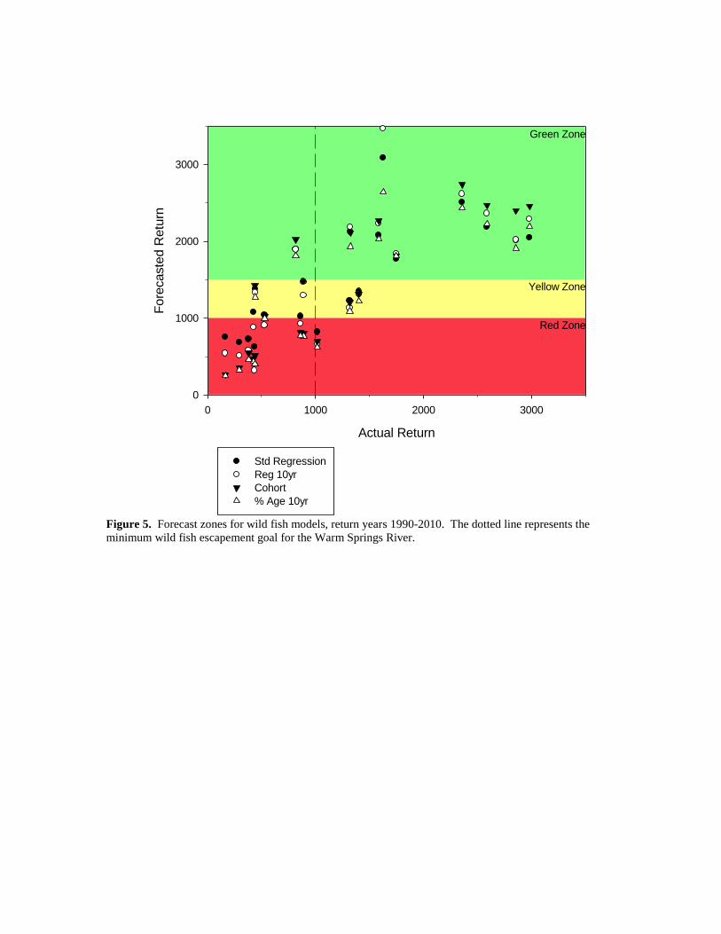
Zone designations were added to the plots of forecasts and actual returns, resulting in
Figure 5. Looking at Figure 5, a general idea of the historic probability of fewer than
1,000 fish returning using a given model’s forecast can be evaluated. Forecasts in the red
zone indicate a high probability of not meeting wild fish escapement goals, forecasts in
the yellow zone a moderate probability of not meeting wild fish escapement goals, and
forecasts in the green zone a low probability of not meeting minimum wild fish
escapement goals. The percent-by-age 10 year model performed the best using the zone
method (Figure 5). Using this model, the forecasted return was in the red zone, i.e. less
than 1,000 adults forecasted, nine times between 1990 and 2010. The actual return of
adults was less than 1,000 (indicated by data points to the left of the dotted line in Figure
5) in eight of those nine years. Fewer than 1,000 wild fish returned in one of three years
the forecast was in the yellow zone, and one out of nine years the forecast was in the
green zone. A summary of zone forecast performance, by forecast model, is shown in
Table 7. Addition of the zone designation to the forecast point estimate in the annual run
prediction reports can be particularly helpful to fishery managers in assessing the risk of
not meeting the minimum escapement goal for wild fish.
Actual Return
0 1000 2000 3000
Fore
caste
d R
etu
rn
0
1000
2000
3000
Std Regression
Reg 10yr
Cohort
% Age 10yr
Green Zone
Yellow Zone
Red Zone
Figure 5. Forecast zones for wild fish models, return years 1990-2010. The dotted line represents the
minimum wild fish escapement goal for the Warm Springs River.

Table 7. Percent of times, given a zone forecast, the actual return of wild spring Chinook
was below 1,000, between 1,000 and 1,500, and above 1,500 adult fish for return years
1990 to 2010. First column (<1,000 actual return) indicates percent of time wild fish
escapement goals were not met when a forecast was in a particular zone. Diagonal values
closest to 100% indicate the best predictor models.
Actual Return
Model
Zone
Forecast <1,000 1,000 to 1,500 >1,500
Standard
Regression
Red 80% 20% 0%
Yellow 71% 29% 0%
Green 11% 11% 78%
Regression
10yr
Red 88% 13% 0%
Yellow 50% 50% 0%
Green 11% 11% 78%
Cohort Red 88% 13% 0%
Yellow 50% 50% 0%
Green 11% 11% 78%
% Age
10yr
Red 89% 11% 0%
Yellow 33% 67% 0%
Green 11% 11% 78%
Hatchery Fish
The percent-by-age model, using all available data, was the best performing model for
hatchery forecasts with a decrease in RMSE value of 20% from the standard regression
model and 31% from the cohort model. In addition, the natural log transformation
decreased the mean percent error from 105% to 68% compared to the standard regression
model. Use of the percent-by-age model and natural log transformed regression model
for forecasts of Warm Springs NFH hatchery spring Chinook salmon returns would have
led to improved forecast accuracy over the years examined in this evaluation. All
models, however, were similar in the forecasting of potential shortfalls for broodstock
(Region D of Figure 4), with the notable exception of the cohort model in return year
1996, when 732 adults returned. The cohort model forecasted an adult return of almost
1,500 in 1996 while all other models forecasted around 1,000 adults.

Recommendations for Warm Springs stock spring Chinook salmon Forecasting in the
Deschutes Basin
Based on the historical data analyzed here, several actions could be taken to improve the
forecasting of spring Chinook salmon returns to the Deschutes basin. Recommendations
for wild fish forecasts are:
Use a 10 year rolling dataset for the standard regression model.
Use the percent-by-age model, with 10 year rolling datasets, to supplement
the traditional forecast models. The percent-by-age model could replace
the cohort model in the run prediction reports.
Add a zone (red, yellow, green) descriptor to the point estimates in run
prediction reports. Forecasts in the red zone would indicate a high
probability of not meeting wild fish escapement goals, in the yellow zone
a moderate probability of not meeting wild fish escapement goals, and in
the green zone a low probability of not meeting minimum wild fish
escapement goals. Statistics, including confidence intervals and
evaluation of past model performance should continue to be included in
run prediction reports.
Continue to evaluate forecast model performance on an annual basis.
Recommendations for Warm Springs NFH hatchery fish forecasts are:
Use natural log transformed data for regression model forecasts.
Use the percent-by-age model to supplement the traditional run forecast
models. The percent-by-age model could replace the cohort model in the
run prediction reports.
Continue to evaluate forecast model performance on an annual basis.

Works Cited
Confederated Tribes of the Warm Springs Reservation of Oregon and United States Fish
& Wildlife Service. 2007. Warm Springs National Fish Hatchery Operational Plan and
Implementation Plan 2007 – 2011. US Fish and Wildlife Service, Vancouver,
Washington.
Haeseker, S.L., R.M. Peterman, and Z. Su. 2008. Retrospective evaluation of preseason
forecasting models for sockeye and chum salmon. North American Journal of Fisheries
Management 28:12-29.
Haeseker, S.L., B. Dorner, R.M. Peterman, and Z. Su. 2007. An improved sibling model
for forecasting chum salmon and sockeye salmon abundance. North American Journal of
Fisheries Management 27:634-642.
Lovtang, J.C., M.W. Gauvin, and D. Hand. 2011. Spring Chinook Salmon in the
Deschutes River, Oregon, Wild and Hatchery. 1975-2009 returns and 2010 Run Size
Forecasts. Prepared by the Confederated Tribes of the Warm Springs Reservation of
Oregon, Oregon Department of Fish & Wildlife, and the U.S. Fish and Wildlife Service.
Warm Springs, Oregon.
Peterman, Randall. 1982. Model of salmon age structure and its use in preseason
forecasting and studies of marine survival. Canadian Journal of Fisheries and Aquatic
Sciences 39:1444-1452.

Appendix 1. Forecast performance measures for wild Warm Springs river spring Chinook salmon forecast models.
Actual Return Std Model Ln Model Cohort Percent by Age
Ret. Year
Age 4
Age 5 Total Pred.
Raw Error
Abs Error
% Error Pred.
Raw Error
Abs Error
% Error Pred.
Raw Error
Abs Error
% Error Pred.
Raw Error
Abs Error
% Error
1979 1,474
1980 1,107 332 1,439
1981 1,205 326 1,531
1982 1,650 413 2,063
1983 1,715 309 2,024
1984 937 255 1,192
1985 1,503 180 1,683
1986 2,160 206 2,366
1987 2,064 496 2,560
1988 1,772 600 2,372
1989 1,641 440 2,081
1990 2,366 488 2,854 2,026 -828 828 -29 2,055 -799 799 -28 2,399 -455 455 -16 2,273 -581 581 -20
1991 864 460 1,324 2,092 768 768 58 2,140 816 816 62 2,114 790 790 60 1,922 598 598 45
1992 1,323 423 1,746 1,825 79 79 5 1,797 51 51 3 1,810 64 64 4 1,715 -31 31 -2
1993 474 416 890 1,481 591 591 66 1,341 451 451 51 805 -85 85 -10 735 -155 155 -17
1994 362 63 425 1,022 597 597 140 782 357 357 84 471 46 46 11 434 9 9 2
1995 94 71 165 732 567 567 343 367 202 202 123 265 100 100 61 251 86 86 52
1996 1,376 24 1,400 1,330 -70 70 -5 1,322 -78 78 -6 1,317 -83 83 -6 1,248 -152 152 -11
1997 826 35 861 1,007 146 146 17 822 -39 39 -5 816 -45 45 -5 762 -99 99 -11
1998 250 44 294 673 379 379 129 389 95 95 32 352 58 58 20 339 45 45 15
1999 365 16 381 717 336 336 88 600 219 219 58 549 168 168 44 491 110 110 29
2000 2,884 98 2,982 2,053 -929 929 -31 2,281 -701 701 -24 2,457 -525 525 -18 2,258 -724 724 -24
2001 1,854 504 2,358 2,472 114 114 5 2,758 400 400 17 2,740 382 382 16 2,491 133 133 6
2002 1,386 199 1,585 2,063 478 478 30 2,248 663 663 42 2,265 680 680 43 2,092 507 507 32
2003 1,249 68 1,317 1,221 -96 96 -7 1,249 -68 68 -5 1,206 -111 111 -8 1,130 -187 187 -14
2004 2,217 370 2,587 2,193 -394 394 -15 2,371 -216 216 -8 2,472 -115 115 -4 2,247 -340 340 -13
2005 793 24 817 1,855 1,038 1,038 127 2,036 1,219 1,219 149 2,025 1,208 1,208 148 1,857 1,040 1,040 127
2006 926 89 1,015 814 -201 201 -20 766 -249 249 -25 694 -321 321 -32 657 -358 358 -35
2007 378 62 440 1,371 931 931 212 1,446 1,006 1,006 229 1,427 987 987 224 1,273 833 833 189
2008 486 43 529 1,038 509 509 96 1,063 534 534 101 1,020 491 491 93 943 414 414 78
2009 399 39 438 623 185 185 42 584 146 146 33 514 76 76 17 460 22 22 5
2010 1,596 31 1,627 3,085 1,458 1,458 90 3,171 1,544 1,544 95 3,582 1,955 1,955 120 3,089 1,462 1,462 90
Mean= 269 509 64 264 469 47 251 416 36 125 375 25

Appendix 2. Forecast performance measures for Warm Springs NFH hatchery Warm Springs river spring Chinook salmon forecast models
Actual Return Std Model Ln Model Cohort Percent by Age Ret. Year
Age 4
Age 5
Total Pred. Raw Error
Abs Error
% Error
Pred. Raw Error
Abs Error
% Error Pred. Raw Error
Abs Error
% Error Pred. Raw Error
Abs Error
% Error
1983 326 115
441
1984 767 20
787
1985 1,508 73
1,581
1986 146 71
217
1987 678 41
719
1988 520 89
609
1989 3,254 89
3,343
1990 1,632 168
1,800
1991 678 139
817
1992 1,080 77
1,157
1993 167 153
320 504 184 184 58 413 93 93 29 254 -66 66 21 199 -121 121 38
1994 27 16
43 388 345 345 802 173 130 130 301 63 20 20 46 45 2 2 5
1995 94 0
94 347 253 253 269 147 53 53 57 84 -10 10 11 58 -36 36 38
1996 731 1
732 986 254 254 35 1,190 458 458 63 1,472 740 740 101 1,003 271 271 37
1997 1,017 29
1046 823 -223 223 21 1,001 -45 45 4 1,114 68 68 7 839 -207 207 20
1998 534 23
557 646 89 89 16 755 198 198 35 715 158 158 28 550 -7 7 1
1999 1,825 47
1872 890 -982 982 52 1,056 -816 816 44 1,216 -656 656 35 909 -963 963 51
2000 9,168 41
9,209 4,788 -4,421 4,421 48 5,126 -4,083 4,083 44 9,052 -157 157 2 6,528 -2,681 2,681 29
2001 4,362 321
4,683 2,956 -1,727 1,727 37 3,347 -1,336 1,336 29 3,507 -1,176 1,176 25 2,926 -1,757 1,757 38
2002 8,074 130
8,204 11,759 3,555 3,555 43 9,068 864 864 11 13,208 5,004 5,004 61 9,813 1,609 1,609 20
2003 6,160 447
6,607 4,851 -1,756 1,756 27 5,252 -1,355 1,355 21 6,456 -151 151 2 5,215 -1,392 1,392 21
2004 4,395 75
4,470 4,446 -24 24 1 4,801 331 331 7 5,624 1,154 1,154 26 4,463 -7 7 0
2005 1,277 118
1395 1,412 17 17 1 1,670 275 275 20 1,615 220 220 16 1,389 -6 6 0
2006 2,697 100
2,797 1,491 -1,306 1,306 47 1,669 -1,128 1,128 40 1,687 -1,110 1,110 40 1,352 -1,445 1,445 52
2007 1,653 223
1876 779 -1,097 1,097 59 821 -1,055 1,055 56 712 -1,164 1,164 62 626 -1,250 1,250 67
2008 2,971 14
2985 6,717 3,732 3,732 125 7,197 4,212 4,212 141 9,313 6,328 6,328 212 6,823 3,838 3,838 129
2009 2,526 97
2623 3,116 493 493 19 3,656 1,033 1,033 39 4,321 1,698 1,698 65 3,415 792 792 30
2010 674 28
702 2,272 1,570 1,570 224 2,664 1,962 1,962 280 2,962 2,260 2,260 322 2,290 1,588 1,588 226
Mean= -58 1,224 105 -12 1,079 68
731 1,230 60 -98 998 45