Embed Size (px)
Citation preview

VOLUME 130 MARCH 2002M O N T H L Y W E A T H E R R E V I E W
q 2002 American Meteorological Society 433
Retrieval of Model Initial Fields from Single-Doppler Observations of a SupercellThunderstorm. Part I: Single-Doppler Velocity Retrieval
STEPHEN S. WEYGANDT,* ALAN SHAPIRO, AND KELVIN K. DROEGEMEIER
Center for Analysis and Prediction of Storms, and School of Meteorology, University of Oklahoma, Norman, Oklahoma
(Manuscript received 23 February 2001, in final form 30 July 2001)
ABSTRACT
In this two-part study, a single-Doppler parameter retrieval technique is developed and applied to a real-datacase to provide initial conditions for a short-range prediction of a supercell thunderstorm. The technique consistsof the sequential application of a single-Doppler velocity retrieval (SDVR), followed by a variational velocityadjustment, a thermodynamic retrieval, and a moisture specification step. By utilizing a sequence of retrievalsin this manner, some of the difficulties associated with full-model adjoints (possible solution nonuniqueness andlarge computational expense) can be circumvented. In Part I, the SDVR procedure and present results from itsapplication to a deep-convective storm are discussed. Part II focuses on the thermodynamic retrieval and sub-sequent numerical prediction.
For the SDVR, Shapiro’s reflectivity conservation-based method is adapted by applying it in a moving referenceframe. Verification of the retrieved wind fields against corresponding dual-Doppler analyses indicates that thebest skill scores are obtained for a reference frame moving with the mean wind, which effectively reduces theproblem to a perturbation retrieval. A decomposition of the retrieved wind field into mean and perturbationcomponents shows that the mean wind accounts for a substantial portion of the total retrieved azimuthal velocity.At low levels, where the retrieval skill scores are especially good, the retrieved perturbation azimuthal velocityis mostly associated with the polar component of vorticity. Missing from the retrieved fields (compared to thedual-Doppler analysis) is most of the low-level azimuthal convergence. Consistent with this result, most of theretrieved updraft is associated with convergence of the perturbation radial velocity, which is calculated fromthe observed radial velocity and directly used in the wind retrieval.
1. Introduction
The installation of the Weather Surveillance Radar-1988 Doppler network (WSR-88D; Klazura and Imy1993) combined with continual increases in computerpower have heightened prospects for the operational im-plementation of numerical models designed to explicitlypredict the evolution of individual thunderstorms andtheir larger aggregates (Lilly 1990; Droegemeier 1990,1997). Toward that end, a significant research effort hasfocused on the development of numerical analysis andprediction techniques suitable for convective-scale phe-nomena and observing systems.
Because Doppler radars are at present the only ob-serving system capable of sampling the detailed flowpatterns within thunderstorms and because the large dis-tance between WSR-88D radars generally precludes
* Current affiliation: NOAA Office of Atmospheric Research, Fore-cast Systems Laboratory, Boulder, Colorado.
Corresponding author address: Stephen S. Weygandt, NOAAForecast Systems Laboratory, 325 Broadway, R/FS1, Boulder, CO80305-3328.E-mail: [email protected]
multiple Doppler wind syntheses, much of the researcheffort has focused on retrieving initial forecast fieldsfrom single-Doppler radar observations. As discussedby Crook (1994), two basic methodologies have beenemployed: those that retrieve all unobserved fields si-multaneously and those that retrieve the three-dimen-sional wind first, followed by a retrieval of the ther-modynamic fields.
The usual approach for retrieving all fields simulta-neously has been to fit a numerical model to a timeseries of observations using four-dimensional variation-al (4DVAR) techniques. The 4DVAR approach hasmany advantages and has become increasingly popularin recent years. The advantages include use of the full-model equations as constraints, simultaneous use of allobservations in their raw form, provision for inclusionof error covariance information, and the ability to re-trieve unobserved fields and find optimal values formodel parameters. The 4DVAR approach may be es-pecially useful for storm-scale retrieval, because it pro-vides potentially the best link between the model-pre-dicted fields and the observations.
The 4DVAR technique was originally developed forsimple models (Lewis and Derber 1985; LeDimet andTalagrand 1986; Talagrand and Courtier 1987) and then

434 VOLUME 130M O N T H L Y W E A T H E R R E V I E W
applied to the problem of initializing large-scale nu-merical models (Navon et al. 1992; Zupanski 1993; The-paut et al. 1993; Zou et al. 1993). Sun et al. (1991)were the first to successfully apply the adjoint techniqueto the single-Doppler retrieval problem. Using a dryBoussinesq model of horizontally periodic Rayleighconvection, they retrieved wind and thermodynamicfields from a single Cartesian velocity component. Real-data tests by Sun and Crook (1994) produced good re-sults for a dry gust-front case. More recently, Sun andCrook (1997, 1998) tested a moist version of their ad-joint retrieval model using both simulated and real radardata observations of a deep-convective storm.
Despite the encouraging results obtained in thesestudies, a number of difficulties have precluded oper-ational implementation of an adjoint-based model ini-tialization procedure for deep-convective storms. First,the severe underdeterminancy and strong nonlinearityof the problem may make it difficult to obtain a unique,converged solution. Second, the many nondifferentiable‘‘on/off’’ switches found in moist physical parameter-izations complicate the construction of accurate tangentlinear and adjoint models (Xu 1996). Third, use of thefull-model equations as a strong constraint neglects themodel error. Finally, the computational expense of nu-merical descent algorithms for finding the minimum ofthe cost function is still prohibitive for real-time appli-cations to deep-convective storms.
The second methodology for obtaining model initialfields from single-Doppler radar observations involvesthe sequential application of a three-dimensional sin-gle-Doppler velocity retrieval (SDVR) followed by athermodynamic retrieval. By applying variational windand thermodynamic retrievals in a sequential manner,it may be possible to circumvent some of the diffi-culties associated with the full-model adjoint tech-niques, while still retaining many of their attributes,including the use of dynamic constraints and time-ten-dency information.
Over the past two decades, a number of methods forretrieving spatially varying wind vectors from a seriesof radar observations have been developed. Early workfocused on techniques for objectively determining themotion of reflectivity or radial velocity features ap-pearing in successive radar scans (Rhinehart 1979; Smy-the and Zrnic 1983; Tuttle and Foote 1990). Implicit inthese techniques was an assumption of reflectivity orradial velocity conservation. More recent techniqueshave utilized a variety of assumptions, including sat-isfaction of simplified prognostic equations for reflec-tivity or radial velocity, mass conservation, spatialsmoothness, velocity stationarity, and frozen turbulence(velocity stationarity in a moving reference frame) en-forced as either strong or weak constraints (Qiu and Xu1992; Xu et al. 1994a,b, 1995; Laroche and Zawadzki1994, 1995; Shapiro et al. 1995a; Zhang and Gal-Chen1996; Xu et al. 2001; Gao et al. 2001).
Another broad class of retrieval procedures has dealt
with the problem of diagnosing thermodynamic fieldsfrom a time history of wind data. Gal-Chen (1978) andHane and Scott (1978) described a least squares tech-nique that obtains pressure deviations from a horizontalaverage using the horizontal momentum equations asweak constraints. Buoyancy perturbations are then ob-tained from the retrieved pressure field using the verticalmomentum equation. Unfortunately, this technique can-not be used to obtain fields of total pressure and buoy-ancy unless a column of independent values is availablefor either pressure or buoyancy. A further limitation ofthe procedure for deep-convective storms is that thetemperature field cannot be obtained from the buoyancyfield unless the moisture fields are known. Inclusion ofa thermodynamic equation in the retrieval (Roux 1985)overcomes the first difficulty, but requires an estimateof the time tendency of the temperature field. Sun andCrook (1996) demonstrated that for dry gust-front casesthe retrieval of thermodynamic fields from a time seriesof three-dimensional wind fields could also be accom-plished using 4DVAR techniques.
In addition to wind and thermodynamic retrievals,procedures have been developed to estimate micro-physical parameters from Doppler radar data. Typicallythey have relied on the availability of a known three-dimensional wind field, such as that obtained from amultiple-Doppler wind analysis. Rutledge and Hobbs(1983, 1984) and Ziegler (1985, 1988) independentlydeveloped techniques in which conservation equationsfor heat and moisture were integrated forward towarda steady state using a prescribed time-invariant windfield. Hauser and Amayenc (1986) inverted steady-stateforms of the conservation equations to obtain micro-physical fields. Verlinde and Cotton (1990) documentedsome of the limitations of the steady-state assumptionand later avoided it by fitting a fully time-dependentkinematic model to idealized observations using the ad-joint technique (Verlinde and Cotton 1993).
Lin et al. (1993) obtained initial forecast fields forthe 20 May 1977 Del City, Oklahoma, tornado case(Ray et al. 1981) by applying a thermodynamic retriev-al to dual-Doppler–derived three-dimensional windfields and making some simple assumptions about themicrophysical variables. Time tendencies of the ve-locity fields were neglected in the thermodynamic re-trieval and retrieved thermodynamic fields were re-tained within regions of hole-filled velocity data. Ashort-range numerical prediction initialized from theretrieved fields was found to evolve faster than theobserved storm. Crook and Tuttle (1994) describe asingle-Doppler initialization procedure that combinesthe tracking reflectivity echoes by correlation wind re-trieval (TREC; Rhinehart 1979) with a thermodynamicretrieval. Use of their procedure to initialize threeshort-range model predictions of dry high plains gustfronts resulted in a modest improvement over a per-sistence forecast.
In essence, this study extends the work of Lin et al.
MARCH 2002 435W E Y G A N D T E T A L .
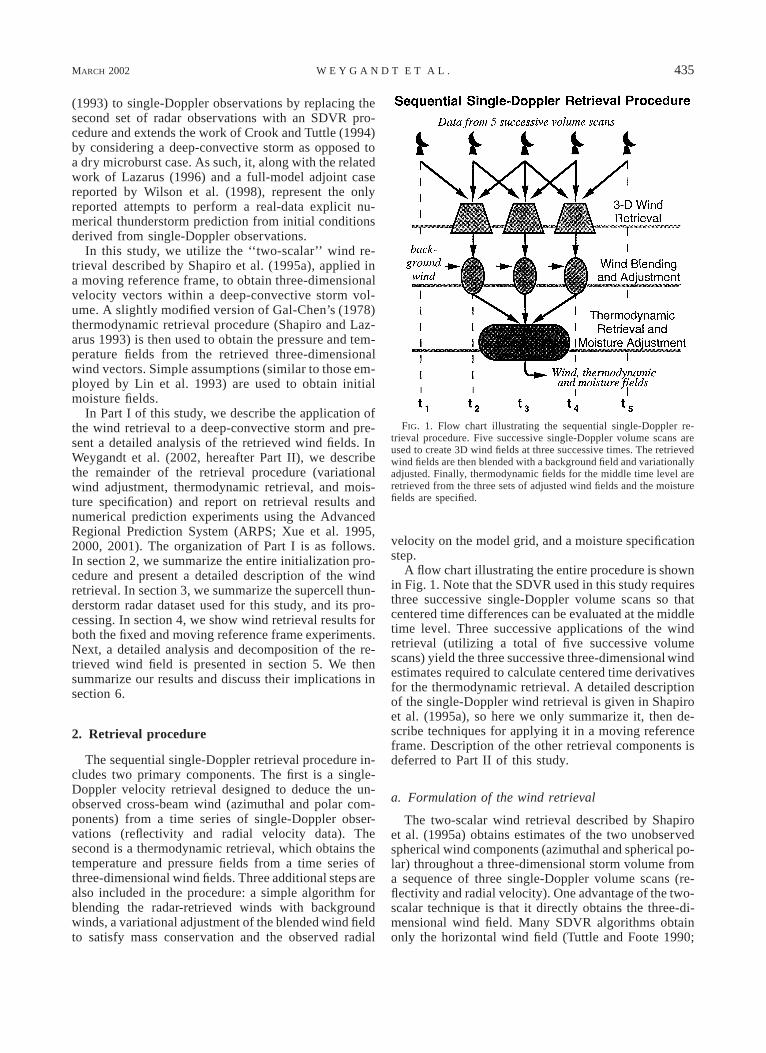
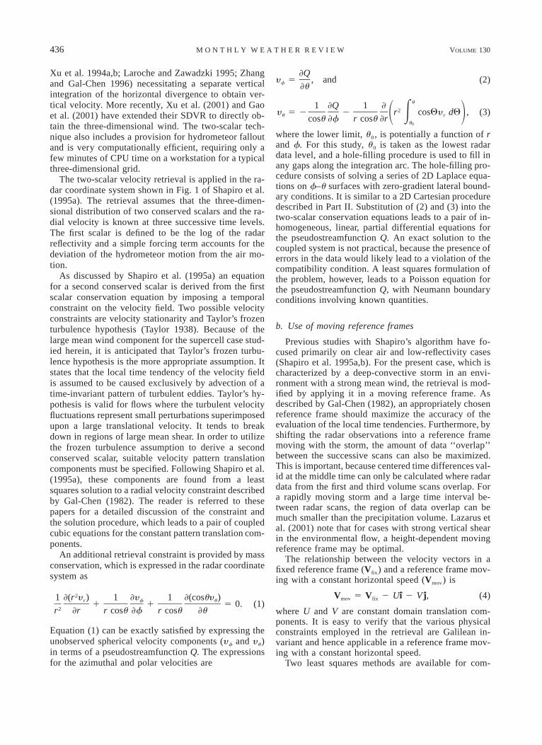
FIG. 1. Flow chart illustrating the sequential single-Doppler re-trieval procedure. Five successive single-Doppler volume scans areused to create 3D wind fields at three successive times. The retrievedwind fields are then blended with a background field and variationallyadjusted. Finally, thermodynamic fields for the middle time level areretrieved from the three sets of adjusted wind fields and the moisturefields are specified.
(1993) to single-Doppler observations by replacing thesecond set of radar observations with an SDVR pro-cedure and extends the work of Crook and Tuttle (1994)by considering a deep-convective storm as opposed toa dry microburst case. As such, it, along with the relatedwork of Lazarus (1996) and a full-model adjoint casereported by Wilson et al. (1998), represent the onlyreported attempts to perform a real-data explicit nu-merical thunderstorm prediction from initial conditionsderived from single-Doppler observations.
In this study, we utilize the ‘‘two-scalar’’ wind re-trieval described by Shapiro et al. (1995a), applied ina moving reference frame, to obtain three-dimensionalvelocity vectors within a deep-convective storm vol-ume. A slightly modified version of Gal-Chen’s (1978)thermodynamic retrieval procedure (Shapiro and Laz-arus 1993) is then used to obtain the pressure and tem-perature fields from the retrieved three-dimensionalwind vectors. Simple assumptions (similar to those em-ployed by Lin et al. 1993) are used to obtain initialmoisture fields.
In Part I of this study, we describe the application ofthe wind retrieval to a deep-convective storm and pre-sent a detailed analysis of the retrieved wind fields. InWeygandt et al. (2002, hereafter Part II), we describethe remainder of the retrieval procedure (variationalwind adjustment, thermodynamic retrieval, and mois-ture specification) and report on retrieval results andnumerical prediction experiments using the AdvancedRegional Prediction System (ARPS; Xue et al. 1995,2000, 2001). The organization of Part I is as follows.In section 2, we summarize the entire initialization pro-cedure and present a detailed description of the windretrieval. In section 3, we summarize the supercell thun-derstorm radar dataset used for this study, and its pro-cessing. In section 4, we show wind retrieval results forboth the fixed and moving reference frame experiments.Next, a detailed analysis and decomposition of the re-trieved wind field is presented in section 5. We thensummarize our results and discuss their implications insection 6.
2. Retrieval procedure
The sequential single-Doppler retrieval procedure in-cludes two primary components. The first is a single-Doppler velocity retrieval designed to deduce the un-observed cross-beam wind (azimuthal and polar com-ponents) from a time series of single-Doppler obser-vations (reflectivity and radial velocity data). Thesecond is a thermodynamic retrieval, which obtains thetemperature and pressure fields from a time series ofthree-dimensional wind fields. Three additional steps arealso included in the procedure: a simple algorithm forblending the radar-retrieved winds with backgroundwinds, a variational adjustment of the blended wind fieldto satisfy mass conservation and the observed radial
velocity on the model grid, and a moisture specificationstep.
A flow chart illustrating the entire procedure is shownin Fig. 1. Note that the SDVR used in this study requiresthree successive single-Doppler volume scans so thatcentered time differences can be evaluated at the middletime level. Three successive applications of the windretrieval (utilizing a total of five successive volumescans) yield the three successive three-dimensional windestimates required to calculate centered time derivativesfor the thermodynamic retrieval. A detailed descriptionof the single-Doppler wind retrieval is given in Shapiroet al. (1995a), so here we only summarize it, then de-scribe techniques for applying it in a moving referenceframe. Description of the other retrieval components isdeferred to Part II of this study.
a. Formulation of the wind retrieval
The two-scalar wind retrieval described by Shapiroet al. (1995a) obtains estimates of the two unobservedspherical wind components (azimuthal and spherical po-lar) throughout a three-dimensional storm volume froma sequence of three single-Doppler volume scans (re-flectivity and radial velocity). One advantage of the two-scalar technique is that it directly obtains the three-di-mensional wind field. Many SDVR algorithms obtainonly the horizontal wind field (Tuttle and Foote 1990;
436 VOLUME 130M O N T H L Y W E A T H E R R E V I E W
Xu et al. 1994a,b; Laroche and Zawadzki 1995; Zhangand Gal-Chen 1996) necessitating a separate verticalintegration of the horizontal divergence to obtain ver-tical velocity. More recently, Xu et al. (2001) and Gaoet al. (2001) have extended their SDVR to directly ob-tain the three-dimensional wind. The two-scalar tech-nique also includes a provision for hydrometeor falloutand is very computationally efficient, requiring only afew minutes of CPU time on a workstation for a typicalthree-dimensional grid.
The two-scalar velocity retrieval is applied in the ra-dar coordinate system shown in Fig. 1 of Shapiro et al.(1995a). The retrieval assumes that the three-dimen-sional distribution of two conserved scalars and the ra-dial velocity is known at three successive time levels.The first scalar is defined to be the log of the radarreflectivity and a simple forcing term accounts for thedeviation of the hydrometeor motion from the air mo-tion.
As discussed by Shapiro et al. (1995a) an equationfor a second conserved scalar is derived from the firstscalar conservation equation by imposing a temporalconstraint on the velocity field. Two possible velocityconstraints are velocity stationarity and Taylor’s frozenturbulence hypothesis (Taylor 1938). Because of thelarge mean wind component for the supercell case stud-ied herein, it is anticipated that Taylor’s frozen turbu-lence hypothesis is the more appropriate assumption. Itstates that the local time tendency of the velocity fieldis assumed to be caused exclusively by advection of atime-invariant pattern of turbulent eddies. Taylor’s hy-pothesis is valid for flows where the turbulent velocityfluctuations represent small perturbations superimposedupon a large translational velocity. It tends to breakdown in regions of large mean shear. In order to utilizethe frozen turbulence assumption to derive a secondconserved scalar, suitable velocity pattern translationcomponents must be specified. Following Shapiro et al.(1995a), these components are found from a leastsquares solution to a radial velocity constraint describedby Gal-Chen (1982). The reader is referred to thesepapers for a detailed discussion of the constraint andthe solution procedure, which leads to a pair of coupledcubic equations for the constant pattern translation com-ponents.
An additional retrieval constraint is provided by massconservation, which is expressed in the radar coordinatesystem as
21 ](r y ) 1 ]y 1 ](cosuy )r f u1 1 5 0. (1)2r ]r r cosu ]f r cosu ]u
Equation (1) can be exactly satisfied by expressing theunobserved spherical velocity components (yf and yu)in terms of a pseudostreamfunction Q. The expressionsfor the azimuthal and polar velocities are
]Qy 5 , and (2)f ]u
u1 ]Q 1 ]2y 5 2 2 r cosQy dQ , (3)u E r1 2cosu ]f r cosu ]r
u0
where the lower limit, u0, is potentially a function of rand f. For this study, u0 is taken as the lowest radardata level, and a hole-filling procedure is used to fill inany gaps along the integration arc. The hole-filling pro-cedure consists of solving a series of 2D Laplace equa-tions on f–u surfaces with zero-gradient lateral bound-ary conditions. It is similar to a 2D Cartesian proceduredescribed in Part II. Substitution of (2) and (3) into thetwo-scalar conservation equations leads to a pair of in-homogeneous, linear, partial differential equations forthe pseudostreamfunction Q. An exact solution to thecoupled system is not practical, because the presence oferrors in the data would likely lead to a violation of thecompatibility condition. A least squares formulation ofthe problem, however, leads to a Poisson equation forthe pseudostreamfunction Q, with Neumann boundaryconditions involving known quantities.
b. Use of moving reference frames
Previous studies with Shapiro’s algorithm have fo-cused primarily on clear air and low-reflectivity cases(Shapiro et al. 1995a,b). For the present case, which ischaracterized by a deep-convective storm in an envi-ronment with a strong mean wind, the retrieval is mod-ified by applying it in a moving reference frame. Asdescribed by Gal-Chen (1982), an appropriately chosenreference frame should maximize the accuracy of theevaluation of the local time tendencies. Furthermore, byshifting the radar observations into a reference framemoving with the storm, the amount of data ‘‘overlap’’between the successive scans can also be maximized.This is important, because centered time differences val-id at the middle time can only be calculated where radardata from the first and third volume scans overlap. Fora rapidly moving storm and a large time interval be-tween radar scans, the region of data overlap can bemuch smaller than the precipitation volume. Lazarus etal. (2001) note that for cases with strong vertical shearin the environmental flow, a height-dependent movingreference frame may be optimal.
The relationship between the velocity vectors in afixed reference frame (Vfix) and a reference frame mov-ing with a constant horizontal speed (Vmov) is
V 5 V 2 Ui 2 V j,mov fix (4)
where U and V are constant domain translation com-ponents. It is easy to verify that the various physicalconstraints employed in the retrieval are Galilean in-variant and hence applicable in a reference frame mov-ing with a constant horizontal speed.
Two least squares methods are available for com-
MARCH 2002 437W E Y G A N D T E T A L .
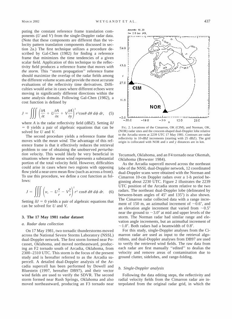
FIG. 2. Locations of the Cimarron, OK (CIM), and Norman, OK,(NOR) radar sites and the crescent-shaped dual-Doppler lobe relativeto the Arcadia storm at 2239 UTC 17 May 1981. Contours are radarreflectivity in 10-dBZ increments (starting with 25 dBZ ). The gridorigin is collocated with NOR and x and y distances are in km.
puting the constant reference frame translation com-ponents (U and V) from the single-Doppler radar data.(Note that these components are different than the ve-locity pattern translation components discussed in sec-tion 2a.) The first technique utilizes a procedure de-scribed by Gal-Chen (1982) for finding a referenceframe that minimizes the time tendencies of a givenscalar field. Application of this technique to the reflec-tivity field produces a reference frame that moves withthe storm. This ‘‘storm propagation’’ reference frameshould maximize the overlap of the radar fields amongthe different volume scans and provide the most accurateevaluations of the reflectivity time derivatives. Diffi-culties would arise in cases where different echoes weremoving in significantly different directions within thesame analysis domain. Following Gal-Chen (1982), acost function is defined by
2]A ]A ]A
2J 5 1 U 1 V r cosu du df dr, (5)EEE 1 2]t ]x ]y
where A is the radar reflectivity field (dBZ). Setting dJ5 0 yields a pair of algebraic equations that can besolved for U and V.
The second procedure yields a reference frame thatmoves with the mean wind. The advantage of this ref-erence frame is that it effectively reduces the retrievalproblem to one of obtaining the unobserved perturba-tion velocity. This would likely be very beneficial insituations where the mean wind represents a substantialportion of the total velocity field. However, difficultiescould arise in cases where two regions with opposingflow yield a near-zero mean flow (such as across a front).To use this procedure, we define a cost function as fol-lows:
2x y2J 5 y 2 U 2 V r cosu du df dr. (6)EEE r1 2r r
Setting dJ 5 0 yields a pair of algebraic equations thatcan be solved for U and V.
3. The 17 May 1981 radar dataset
a. Radar data collection
On 17 May 1981, two tornadic thunderstorms movedacross the National Severe Storms Laboratory (NSSL)dual-Doppler network. The first storm formed near Po-casset, Oklahoma, and moved northeastward, produc-ing an F2 tornado south of Arcadia, Oklahoma, from2300–2310 UTC. This storm is the focus of the presentstudy and is hereafter referred to as the Arcadia su-percell. A detailed dual-Doppler analysis of the Ar-cadia supercell has been performed by Dowell andBluestein (1997, hereafter DB97), and their vectorwind fields are used to verify the SDVR. The secondstorm formed near Rush Springs, Oklahoma and alsomoved northeastward, producing an F3 tornado near
Tecumseh, Oklahoma, and an F4 tornado near Okemah,Oklahoma (Brewster 1984).
As the Arcadia supercell moved across the northeastlobe of the NSSL dual-Doppler network, 12 coordinateddual-Doppler scans were obtained with the Norman andCimarron 10-cm Doppler radars over a 1-h period be-ginning about 2230 UTC. Figure 2 illustrates the 2239UTC position of the Arcadia storm relative to the tworadars. The northeast dual-Doppler lobe (delineated bybetween-beam angles of 458 and 1358) is also shown.The Cimarron radar collected data with a range incre-ment of 150 m, an azimuthal increment of ;0.68, andan elevation angle increment that varied from ;0.58near the ground to ;3.08 at mid and upper levels of thestorm. The Norman radar had similar range and ele-vation angle increments, but an azimuthal increment of;1.08. Both radars had a beamwidth of 0.88.
For this study, single-Doppler analyses from the Ci-marron radar are used as input to the retrieval algo-rithms, and dual-Doppler analyses from DB97 are usedto verify the retrieved wind fields. The raw data fromeach radar are first manually ‘‘edited’’ to dealias thevelocity and remove areas of contamination due toground clutter, sidelobes, and range-folding.
b. Single-Doppler analysis
Following the data editing steps, the reflectivity andradial velocity fields from the Cimarron radar are in-terpolated from the original radar grid, in which the
438 VOLUME 130M O N T H L Y W E A T H E R R E V I E W
azimuthal increments vary slightly, to a new sphericalgrid on which the SDVR is applied. The new grid hasa constant azimuthal increment of Df 5 28, a constantrange increment of Dr 5 1 km, and the original ele-vation angle increments. A 2D Cressman (1959) algo-rithm with a circular influence region in the r–f planeis used to map the fields to the new grid.
Because our goal in analyzing fields for input to theSDVR (defined on the new spherical grid) is to retainfeatures with a constant grid-relative wavelength, a spe-cial procedure for calculating range-dependent radii ofinfluence is used in the Cressman algorithm. The prin-ciple underlying this procedure is to force the radii ofinfluence to be locally isotropic, while allowing the sizeof the influence region to increase with increasing rangeto match the variable grid resolution inherent in spher-ical grids. Using the resultant fields, the SDVR can max-imize detail at close range without producing excessivesmall-scale noise at far range. While appropriate for thisapplication, Trapp and Doswell (2000) caution that non-homogeneous radii of influence should not be used forstudies in which the magnitudes of different radar-an-alyzed features are compared. Because the analyzedmagnitude of a feature is a convolution of the radarobserved strength with the analysis weight function, anartificial spatial dependence can be introduced by usingspatially varying weight functions.
To obtain expressions for the desired radii of influ-ence, we first define a constant aspect ratio between theradii of influence in the range and azimuthal directions:
a 5 L /L ,r f (7)
where Lr and Lf are the radii of influence in the rangeand azimuthal directions. Local isotropy is enforced bysetting a 5 1, yielding a circular influence region. Thephysical distances Lr and Lf are related to the corre-sponding gridpoint distances by
L 5 N Dr, and (8)r r
L 5 N rDf, (9)f f
where Nr and Nf are the fractional number of analysisgrid points in the range and azimuthal radii of influence,respectively. Next, the product NrNf is held constantfor all r, resulting in an influence area that increaseswith increasing radar range. An expression for Lr as afunction of range can be derived starting from a generalformula for the area of the influence ellipse:
pL L 5 prN N DrDf.r f r f (10)
Using (7) to eliminate Lf in (10) and solving for Lr
leads to1/2L 5 Kr ,r (11)
where1/2K 5 (aN N DrDf)r f
is constant for all values of radar range.
To utilize this formulation, a physical distance for therange radius of influence is specified for some referencerange. Then, Nr and Nf can be calculated for the ref-erence range from (8) and (9). Next, the constant, K, isdetermined and Lr is calculated for all values of rangeusing (11). As a last step, Nr and Nf are computed forall values of range, using (8) and (9). Note that Nr andNf apply to the analysis grid, and the physical distancesLr and Lf must be used to determine which radar datapoints lie within the influence region of a given analysispoint. For this study, values of 20 km and 1.8 km werechosen for the reference range and range radius of in-fluence at that reference range.
c. Dual-Doppler verification
Dual-Doppler analyses of the Arcadia supercell fromDB97 are used to verify the single-Doppler retrievalresults. The reader is referred to DB97 for a detaileddescription of the analysis procedure; only a brief sum-mary is provided here. First, the raw radar data areinterpolated to a common uniform Cartesian grid (Dx5 Dy 5 0.8 km, Dz 5 0.5 km) using a Cressman (1959)scheme with a spherical influence radius of 1.2 km. Inthis procedure, data from the lowest elevation angle areextrapolated to the ground. Next, a dual-equation systemis iteratively solved in conjunction with a downwardintegration of the anelastic mass conservation equationto obtain vertical velocities. A boundary condition ofw 5 0 at the top of each data column was used for thedownward integration, and an O’Brien (1970) correctionwas applied to ensure vertical velocities of zero at theground and data column top.
It is important to note that inaccuracies associatedwith the assumed upper boundary condition, as well asthe extrapolation of data from the lowest elevation angleto the ground, may lead to substantial errors in the com-puted vertical velocity. Because of these possible errors,quantitative verification of the single-Doppler retrievalagainst the dual-Doppler analysis is only performed forthe azimuthal velocity. Note also that verifying the az-imuthal velocity, which is completely unobserved bythe ‘‘input’’ radar, is more rigorous than verifying thetotal horizontal wind, which includes a portion of theobserved radial velocity.
The verification is accomplished by first trilinearlyinterpolating both the SDVR and dual-Doppler windfields to a common unstaggered Cartesian grid. To fa-cilitate the thermodynamic retrieval and model predic-tions described in Part II of this study, the common gridis chosen to be the scalar points of the ARPS modelgrid, with constant horizontal and vertical grid spacingsof 1.0 km and 0.5 km, respectively. Two quantitativeskill scores, the root-mean-square error and the linearcorrelation coefficient, are then calculated for the re-trieved azimuthal velocity.
MARCH 2002 439W E Y G A N D T E T A L .
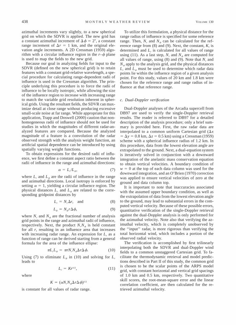
TABLE 1. Comparison of the moving reference frame translationcomponents (m s21) calculated from the single-Doppler data with thecorresponding verification values for the three successive retrievaltimes.
Reference framecomponent
Time
2234UTC
2239UTC
2243UTC Avg
Storm propagationSingle-Doppler UVerification U
7.47.8
6.98.5
8.011.4
7.49.2
Single-Doppler VVerification V
5.34.9
5.64.7
5.75.7
5.55.1
Mean windSingle-Doppler UVerification U
22.421.6
22.421.1
21.921.7
22.421.5
Single-Doppler VVerification V
12.914.3
13.013.4
13.413.7
13.113.8
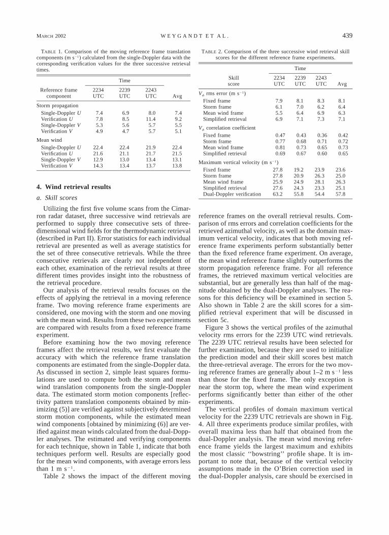
TABLE 2. Comparison of the three successive wind retrieval skillscores for the different reference frame experiments.
Skillscore
Time
2234UTC
2239UTC
2243UTC Avg
Vf rms error (m s21)Fixed frameStorm frameMean wind frameSimplified retrieval
7.96.15.56.9
8.17.06.47.1
8.36.26.97.3
8.16.46.37.1
Vf correlation coefficientFixed frameStorm frameMean wind frameSimplified retrieval
0.470.770.810.69
0.430.680.730.67
0.360.710.650.60
0.420.720.730.65
Maximum vertical velocity (m s21)Fixed frameStorm frameMean wind frameSimplified retrievalDual-Doppler verification
27.827.825.927.663.2
19.220.924.924.355.8
23.926.328.123.354.4
23.625.026.325.157.8
4. Wind retrieval results
a. Skill scores
Utilizing the first five volume scans from the Cimar-ron radar dataset, three successive wind retrievals areperformed to supply three consecutive sets of three-dimensional wind fields for the thermodynamic retrieval(described in Part II). Error statistics for each individualretrieval are presented as well as average statistics forthe set of three consecutive retrievals. While the threeconsecutive retrievals are clearly not independent ofeach other, examination of the retrieval results at threedifferent times provides insight into the robustness ofthe retrieval procedure.
Our analysis of the retrieval results focuses on theeffects of applying the retrieval in a moving referenceframe. Two moving reference frame experiments areconsidered, one moving with the storm and one movingwith the mean wind. Results from these two experimentsare compared with results from a fixed reference frameexperiment.
Before examining how the two moving referenceframes affect the retrieval results, we first evaluate theaccuracy with which the reference frame translationcomponents are estimated from the single-Doppler data.As discussed in section 2, simple least squares formu-lations are used to compute both the storm and meanwind translation components from the single-Dopplerdata. The estimated storm motion components [reflec-tivity pattern translation components obtained by min-imizing (5)] are verified against subjectively determinedstorm motion components, while the estimated meanwind components [obtained by minimizing (6)] are ver-ified against mean winds calculated from the dual-Dopp-ler analyses. The estimated and verifying componentsfor each technique, shown in Table 1, indicate that bothtechniques perform well. Results are especially goodfor the mean wind components, with average errors lessthan 1 m s21.
Table 2 shows the impact of the different moving
reference frames on the overall retrieval results. Com-parison of rms errors and correlation coefficients for theretrieved azimuthal velocity, as well as the domain max-imum vertical velocity, indicates that both moving ref-erence frame experiments perform substantially betterthan the fixed reference frame experiment. On average,the mean wind reference frame slightly outperforms thestorm propagation reference frame. For all referenceframes, the retrieved maximum vertical velocities aresubstantial, but are generally less than half of the mag-nitude obtained by the dual-Doppler analyses. The rea-sons for this deficiency will be examined in section 5.Also shown in Table 2 are the skill scores for a sim-plified retrieval experiment that will be discussed insection 5c.
Figure 3 shows the vertical profiles of the azimuthalvelocity rms errors for the 2239 UTC wind retrievals.The 2239 UTC retrieval results have been selected forfurther examination, because they are used to initializethe prediction model and their skill scores best matchthe three-retrieval average. The errors for the two mov-ing reference frames are generally about 1–2 m s21 lessthan those for the fixed frame. The only exception isnear the storm top, where the mean wind experimentperforms significantly better than either of the otherexperiments.
The vertical profiles of domain maximum verticalvelocity for the 2239 UTC retrievals are shown in Fig.4. All three experiments produce similar profiles, withoverall maxima less than half that obtained from thedual-Doppler analysis. The mean wind moving refer-ence frame yields the largest maximum and exhibitsthe most classic ‘‘bowstring’’ profile shape. It is im-portant to note that, because of the vertical velocityassumptions made in the O’Brien correction used inthe dual-Doppler analysis, care should be exercised in
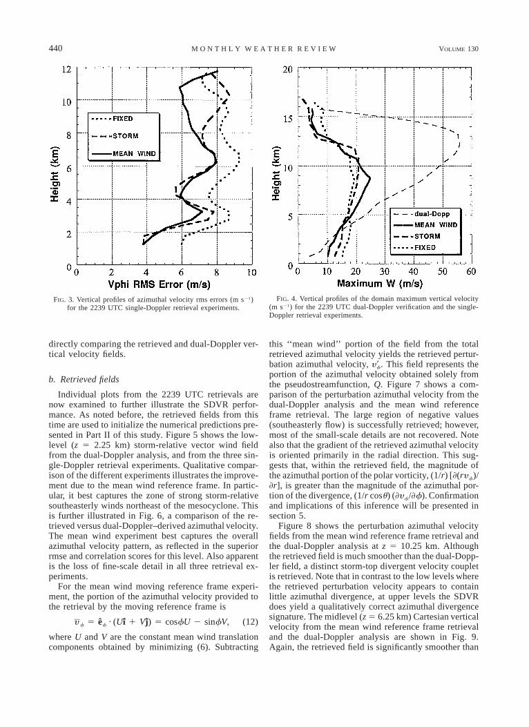
440 VOLUME 130M O N T H L Y W E A T H E R R E V I E W
FIG. 3. Vertical profiles of azimuthal velocity rms errors (m s21)for the 2239 UTC single-Doppler retrieval experiments.
FIG. 4. Vertical profiles of the domain maximum vertical velocity(m s21) for the 2239 UTC dual-Doppler verification and the single-Doppler retrieval experiments.
directly comparing the retrieved and dual-Doppler ver-tical velocity fields.
b. Retrieved fields
Individual plots from the 2239 UTC retrievals arenow examined to further illustrate the SDVR perfor-mance. As noted before, the retrieved fields from thistime are used to initialize the numerical predictions pre-sented in Part II of this study. Figure 5 shows the low-level (z 5 2.25 km) storm-relative vector wind fieldfrom the dual-Doppler analysis, and from the three sin-gle-Doppler retrieval experiments. Qualitative compar-ison of the different experiments illustrates the improve-ment due to the mean wind reference frame. In partic-ular, it best captures the zone of strong storm-relativesoutheasterly winds northeast of the mesocyclone. Thisis further illustrated in Fig. 6, a comparison of the re-trieved versus dual-Doppler–derived azimuthal velocity.The mean wind experiment best captures the overallazimuthal velocity pattern, as reflected in the superiorrmse and correlation scores for this level. Also apparentis the loss of fine-scale detail in all three retrieval ex-periments.
For the mean wind moving reference frame experi-ment, the portion of the azimuthal velocity provided tothe retrieval by the moving reference frame is
y 5 e · (Ui 1 Vj) 5 cosfU 2 sinfV,f f (12)
where U and V are the constant mean wind translationcomponents obtained by minimizing (6). Subtracting
this ‘‘mean wind’’ portion of the field from the totalretrieved azimuthal velocity yields the retrieved pertur-bation azimuthal velocity, . This field represents they9fportion of the azimuthal velocity obtained solely fromthe pseudostreamfunction, Q. Figure 7 shows a com-parison of the perturbation azimuthal velocity from thedual-Doppler analysis and the mean wind referenceframe retrieval. The large region of negative values(southeasterly flow) is successfully retrieved; however,most of the small-scale details are not recovered. Notealso that the gradient of the retrieved azimuthal velocityis oriented primarily in the radial direction. This sug-gests that, within the retrieved field, the magnitude ofthe azimuthal portion of the polar vorticity, (1/r) [](ryf)/]r], is greater than the magnitude of the azimuthal por-tion of the divergence, (1/r cosu) (]yf/]f). Confirmationand implications of this inference will be presented insection 5.
Figure 8 shows the perturbation azimuthal velocityfields from the mean wind reference frame retrieval andthe dual-Doppler analysis at z 5 10.25 km. Althoughthe retrieved field is much smoother than the dual-Dopp-ler field, a distinct storm-top divergent velocity coupletis retrieved. Note that in contrast to the low levels wherethe retrieved perturbation velocity appears to containlittle azimuthal divergence, at upper levels the SDVRdoes yield a qualitatively correct azimuthal divergencesignature. The midlevel (z 5 6.25 km) Cartesian verticalvelocity from the mean wind reference frame retrievaland the dual-Doppler analysis are shown in Fig. 9.Again, the retrieved field is significantly smoother than

MARCH 2002 441W E Y G A N D T E T A L .
FIG. 5. The 2239 UTC low-level (z 5 2.25 km) reflectivity and storm-relative horizontal vectors for (a) the dual-Doppler analysis, andthe retrieval performed in (b) the mean wind reference frame, (c) the storm propagation reference frame, and (d) the fixed reference frame.Reflectivity is contoured every 10 dBZ. Grid distances are in km and CIM (input) is located at x 5 25, y 5 10.
its dual-Doppler counterpart, but captures the principalfeatures reasonably well. In particular, the horseshoe-shaped updraft maximum surrounding the primary ver-tical velocity minimum is reproduced. The vertical ve-locity field in the other reference frame experiments (notshown) is remarkably similar to that of the mean windreference frame retrieval.
5. Analysis of the retrieved wind fields
In addition to illustrating the superiority of the meanwind reference frame retrieval, the results presented inthe previous section reveal a number of intriguing fea-tures. First, for all three reference frame experiments,the spatial patterns of the retrieved vertical velocity
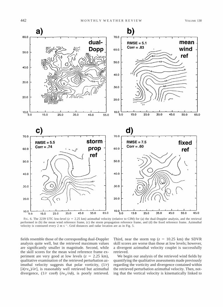
442 VOLUME 130M O N T H L Y W E A T H E R R E V I E W
FIG. 6. The 2239 UTC low-level (z 5 2.25 km) azimuthal velocity (relative to CIM) for (a) the dual-Doppler analysis, and the retrievalperformed in (b) the mean wind reference frame, (c) the storm propagation reference frame, and (d) the fixed reference frame. Azimuthalvelocity is contoured every 2 m s21. Grid distances and radar location are as in Fig. 5.
fields resemble those of the corresponding dual-Doppleranalysis quite well, but the retrieved maximum valuesare significantly smaller in magnitude. Second, whilethe skill scores for the mean wind reference frame ex-periment are very good at low levels (z 5 2.25 km),qualitative examination of the retrieved perturbation az-imuthal velocity suggests that polar vorticity, (1/r)[](ryf)/]r], is reasonably well retrieved but azimuthaldivergence, (1/r cosu) (]yf/]f), is poorly retrieved.
Third, near the storm top (z 5 10.25 km) the SDVRskill scores are worse than those at low levels; however,a divergent azimuthal velocity couplet is successfullyretrieved.
We begin our analysis of the retrieved wind fields byquantifying the qualitative assessments made previouslyregarding the vorticity and divergence contained withinthe retrieved perturbation azimuthal velocity. Then, not-ing that the vertical velocity is kinematically linked to
MARCH 2002 443W E Y G A N D T E T A L .
FIG. 7. The 2239 UTC low-level (z 5 2.25 km) perturbation azi-muthal velocity (relative to CIM) for (a) the dual-Doppler analysis and(b) the retrieval performed in the mean wind reference frame. Thecontour interval, grid distances, and radar location are as in Fig. 6.
the vertical profile of horizontal divergence, a verticalvelocity decomposition is performed to help explain thevertical velocity results. Finally, results from the fullretrieval will be compared with a drastically simplifiedretrieval suggested to us by the vertical velocity decom-position.
a. Vorticity and divergence calculations
The three-dimensional vorticity vector in radar co-ordinates is
1 ](cosuy ) ]y 1 ](ry ) ]yf u u rv 5 e 2 1 e 2r f[ ] [ ]r cosu ]u ]f r ]r ]u
1 1 ]y ](ry )r f1 e 2 (13)u [ ]r cosu ]f ]r
and the three-dimensional divergence, = ·V 5 ]u/]x 1]y/]y 1 ]w/]z, in radar coordinates is given by (1). Forthe case of a constant horizontal wind (V 5 Uı 1 Vj),each of the three terms that comprise the three-dimen-sional divergence will be zero in a Cartesian coordinatesystem. However, in the radar (spherical) coordinatesystem, the three terms that sum to give the three-di-mensional divergence are not each identically zero.Rather, cancellation occurs between the terms, resultingin a three-dimensional divergence of zero. A similarsituation occurs in the calculation of the vorticity com-ponents for a mean horizontal wind. In a Cartesian co-ordinate system, both the vertical component of vorticityand the two terms that comprise it are zero. In contrast,for the radar coordinate system (consider the limitingcase of zero elevation angle) the radial and azimuthalcontributions to the polar vorticity component are notzero, but cancel each other, resulting in zero polar vor-ticity. While mathematically correct, these nonzeromean wind terms complicate the interpretation of di-vergence and vorticity estimates obtained from Dopplerradar data. These complications are discussed in theappendix, where it is shown that vorticity and diver-gence calculations involving spherical velocity com-ponents derived from radar observations should be per-formed using perturbation velocity fields (i.e., fields inwhich the contribution of the mean horizontal wind tothe spherical components is subtracted out prior to thecalculations). These mean wind contributions can beseen in the relationship between the total, mean, andperturbation spherical velocities:
y 5 y 1 y9 5 cosu sinfU 1 cosu cosfV 1 y9, (14)r r r r
y 5 y 1 y9 5 cosfU 2 sinfV 1 y9 , and (15)f f f f
y 5 y 1 y9 5 2sinu sinfU 2 sinu cosfV 1 y9. (16)u u u u
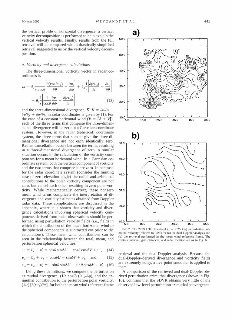
Using these definitions, we compute the perturbationazimuthal divergence, (1/r cosu) (] /]f), and the az-y9fimuthal contribution to the perturbation polar vorticity,(1/r) [](r )/]r], for both the mean wind reference framey9f
retrieval and the dual-Doppler analysis. Because thedual-Doppler–derived divergence and vorticity fieldsare extremely noisy, a five-point smoother is applied tothem.
A comparison of the retrieved and dual-Doppler–de-rived perturbation azimuthal divergence (shown in Fig.10), confirms that the SDVR obtains very little of theobserved low-level perturbation azimuthal convergence.

444 VOLUME 130M O N T H L Y W E A T H E R R E V I E W
FIG. 8. The 2239 UTC upper-level (z 5 10.25 km) perturbationazimuthal velocity (relative to CIM) for (a) the dual-Doppler analysisand (b) the retrieval performed in the mean wind reference frame. Thecontour interval, grid distances, and radar location are as in Fig. 6.
In fact, the retrieved field shows weak divergence in thesouthwest portion of the storm, whereas the dual-Dopp-ler verification show strong convergence associated withthe low-level inflow into the main updraft. As will beshown, this is consistent with the substantially weakerretrieved updraft maximum compared with the dual-Doppler analysis.
In contrast, the retrieved azimuthal contribution tothe perturbation polar vorticity field (Fig. 11b) bettermatches its dual-Doppler counterpart (Fig. 11a). Notethat although the retrieved extrema are smaller than theverification extrema, the zero lines and location of themaximum near x 5 20, y 5 30 match quite well. Takenin conjunction with Fig. 3, which shows this level tohave nearly the best rms scores, it is concluded that, atlow levels, the SDVR retrieves the azimuthal contri-bution to the perturbation polar vorticity reasonablywell, but retrieves very little of the observed pertur-bation azimuthal convergence.
b. Vertical velocity decomposition
Results from a vertical velocity decomposition arenow presented to illustrate the contribution of the re-trieved perturbation azimuthal divergence to the re-trieved updraft strength. Starting with (1), the expres-sion for mass conservation in radar coordinates, weintegrate the r–f divergence in the polar direction toget
ucosu 1 ]0 2y 5 y 2 r cosQy dQu u E r0 1 2cosu r cosu ]ru0
u1 ]2 y dQ . (17)E f1 2cosu ]f
u0
Defining a mean wind to be that used by the SDVR forthe moving reference frame, the radial, azimuthal, andpolar velocity components (y r, yf, yu) can be partitionedinto mean and perturbation parts using (14)–(16). Sub-stituting these mean and perturbation parts into (17) andevaluating the integrals involving the mean wind terms(see appendix for details) leads to
ucosu 1 ]0 2y 5 y9 2 r cosQy9 dQu u E r0 1 2cosu r cosu ]ru0
u1 ]2 y9 dQE f1 2cosu ]f
u0
2 sinu(sinfU 1 cosfV ). (18)
The Cartesian vertical velocity component can be ex-pressed in terms of the radial and polar velocity com-ponents as
w 5 sinuy 1 cosuy .r u (19)
Substitution of (14) and (18) into (19) leads to an ex-pression for the Cartesian vertical velocity componentin terms of the perturbation spherical velocity compo-nents,

MARCH 2002 445W E Y G A N D T E T A L .
FIG. 9. The 2239 UTC midlevel (z 5 6.25 km) vertical velocityfor (a) the dual-Doppler analysis and (b) the retrieval performed inthe mean wind reference frame. The contour interval, grid distances,and radar location are as in Fig. 6.
u1 ]2w 5 sinuy9 1 cosu y9 2 r cosQy9 dQr 0 u E r0 1 2r ]r
u0
u]2 y9 dQ . (20)E f1 2]f
u0
Equation (20) is analogous to the Cartesian expression
for vertical velocity in terms of the vertical integral ofthe horizontal divergence:
z z] ]w 5 w 2 u dZ 2 y dZ , (21)z E E0 1 2 1 2]x ]yz z0 0
and is especially relevant to our present analysis of theSDVR results, because it relates the Cartesian verticalvelocity to terms involving the observed radial velocityand retrieved cross-beam velocity. The last two termsin (20) are the contributions from the radial divergence(which can be calculated from the observed radial ve-locity) and the azimuthal divergence (which can be cal-culated from the retrieved azimuthal velocity). As dis-cussed in the appendix, the terms on the right-hand sideof (20) involve only perturbation quantities, because themean wind portions of these terms have been separatedout and summed to zero.
The first term on the rhs of (20) is the vertical pro-jection of the perturbation radial velocity. It can be di-rectly obtained from observed radial velocity (given theestimated mean wind), and is usually small. The secondterm on the rhs of (20) is the lower-boundary conditionfor the polar velocity component and is analogous tothe lower boundary condition on w in the Cartesianvertical velocity expression. Note that this lower bound-ary condition is at the lower boundary of the data cov-erage region, not necessarily at the ground. One of theadvantages of the two-scalar retrieval algorithm is thatit implicitly obtains this term by directly retrieving avalue for the polar velocity at the lowest data level. Forretrieval schemes that do not obtain this term (or anal-ogous terms in other coordinate systems), the difficultiesof applying boundary conditions above the ground mustbe faced.
The contribution from each of the divergence termstoward the total retrieved vertical velocity can be com-puted at any level by integrating upward along an arcof constant range and azimuth. Fortunately, the mainupdraft in the Arcadia storm has a fairly large horizontalextension, allowing an arc to be found that lies almostentirely within the storm updraft. Figure 12 shows theprofiles of the retrieved vertical velocity and the variousterms in the decomposition along such an arc. The moststriking result is that retrieved vertical velocity is as-sociated almost entirely with the convergence of per-turbation radial velocity, which is directly computedfrom the observed radial velocity (after subtracting theestimated mean wind) in the retrieval. Consistent withFig. 10, which showed that the retrieval obtains weakazimuthal divergence at low levels, the contribution tothe retrieved vertical velocity from the azimuthal di-vergence term is actually slightly negative at low levels.Note also that the retrieval obtains a reasonable valueof about 13 m s21 for the lower boundary conditionterm.

446 VOLUME 130M O N T H L Y W E A T H E R R E V I E W
c. Comparison with a simplified retrieval
The results from the wind decomposition suggest adrastically simplified retrieval against which we nowcompare the full SDVR. The drastically simplifiedretrieval retains only those terms that can be directlyobtained from the observed radial velocity, and ne-glects those terms that require solution of the Poissonequation for Q. The various terms can be explicitlywritten by noting that application of the SDVR in amean wind moving reference frame is equivalent toperforming a perturbation retrieval. Thus (2) and (3)become
]Q9y9 5 , (22)f ]u
u1 ]Q9 1 ]2y9 5 2 2 r cosQy9 dQ , (23)u E r1 2cosu ]f r cosu ]r
u0
where Q9 is a perturbation pseudostreamfunction. Sub-stitution of these expressions into (15) and (16) resultsin a useful decomposition of the unobserved sphericalcomponents:
]Q9y 5 y 1 y9 5 cosfU 2 sinfV 1 , and (24)f f f ]u
y 5 y 1 y9 5 2sinu sinfU 2 sinu cosfVu u u
u1 ] 1 ]Q922 r cosQy9 dQ 2 . (25)E r1 2r cosu ]r cosu ]f
u0
Noting that the horizontal mean wind components areobtained from the radial velocity [by minimizing (6)],we see that the simplified retrieval retains all but thefinal term in each of (24) and (25) (i.e., the terms in-volving Q9). This simplified retrieval is not offered asan alternative to the full retrieval, but as a reference forassessing the relative contributions from the perturba-tion pseudostreamfunction and the terms directly ob-tainable from the radial velocity.
It is important to note that the perturbation radialdivergence, the integrand appearing in (25), could beused to obtain a portion of the azimuthal velocity insteadof the polar velocity. Thus, while the results of the sim-ple retrieval depend on the direction in which we chooseto integrate the radial divergence, the results from thetwo-scalar retrieval are independent of this choice.
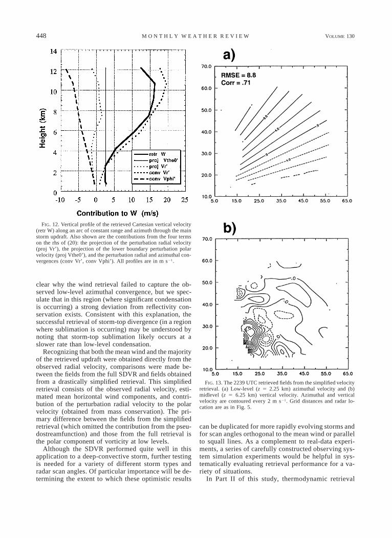
Figure 13a illustrates that the azimuthal velocity ob-tained by this simple retrieval is merely the local pro-jection of the mean horizontal wind in the azimuthaldirection. Consistent with Fig. 12, the retrieved verticalvelocity field (Fig. 13b) is very similar to that from theother experiments. Given that the bulk of the verticalvelocity is obtained from the perturbation radial con-vergence, it is now clear why all the experiments obtainsimilar vertical velocities.
Returning to Table 2, we see that the drastically sim-plified retrieval clearly outperforms the fixed reference
frame experiment. Skill scores for both of the movingreference frame experiments are better, however, indi-cating that although the mean horizontal wind containsmuch of the azimuthal velocity field, use of either ofthe two moving reference frames yields a perturbationazimuthal velocity that adds skill relative to the sim-plified wind retrieval. In Part II, we assess the effect ofthese perturbation fields on the subsequent thermody-namic retrieval and numerical prediction.
6. Summary and discussion
In this two-part study, a single-Doppler parameterretrieval technique is developed and applied to a real-data case to provide model initial conditions for a short-range prediction of a supercell thunderstorm. The tech-nique consists of the sequential application of a single-Doppler velocity retrieval, followed by a variational ve-locity adjustment and a thermodynamic retrieval. In PartI of the study, we have described the SDVR and tech-niques for applying it in a moving reference frame. Twopossible moving reference frames were considered: onethat follows the storm motion and one that follows themean wind. For each of these moving reference frames,we presented simple variational procedures for esti-mating the horizontal translation components.
The SDVR was used to retrieve the complete three-dimensional wind field within a deep-convective stormfrom a time series of single-Doppler radar observa-tions. Verification of the retrieved wind fields was ac-complished by comparing them with correspondingdual-Doppler analyses. For each of the two movingreference frames considered, the simple variationalprocedure obtained the horizontal translation compo-nents with a high degree of accuracy. Application ofthe retrieval in either of the moving reference framessignificantly improved the results compared with thefixed frame. The best results, however, were obtainedfor the mean wind moving reference frame, which ef-fectively reduced the problem to one of retrieving theunobserved perturbation velocity. For the mean windmoving reference frame case, the correlation coeffi-cient between the retrieved and dual-Doppler–derivedazimuthal velocity (averaged over the entire 3D stormvolume) ranged from 0.65 to 0.81 for three successiveapplications of the retrieval.
A decomposition of the retrieved azimuthal velocityindicated that the projection of the mean wind movingreference frame components accounted for a substantialportion of the total retrieved azimuthal velocity. Sub-tracting this azimuthal projection of the estimated meanwind from the retrieved azimuthal velocity allowed acomparison of the retrieved and verifying perturbationazimuthal velocity fields. At low levels, the retrievedperturbation azimuthal velocity was associated mostlywith polar vorticity, and exhibited weak azimuthal di-vergence. In contrast, the dual-Doppler verification con-tained strong azimuthal convergence at low levels. Con-

MARCH 2002 447W E Y G A N D T E T A L .
FIG. 10. The 2239 UTC low-level (z 5 2.25 km) perturbationazimuthal divergence (1023 s21) for (a) the dual-Doppler analysisand (b) the retrieval performed in the mean wind reference frame.The contour interval is 0.5 3 1023 s21. Grid distances and radarlocation are as in Fig. 5.
FIG. 11. The 2239 UTC low-level (z 5 2.25 km) perturbationazimuthal contribution to polar vorticity (1023 s21) for (a) the dual-Doppler analysis and (b) the retrieval performed in the mean windreference frame. The contour interval is 0.5 3 1023 s21. Grid dis-tances and radar location are as in Fig. 5.
sistent with this, the retrieved updraft maximum of 25m s21 was slightly less than half of the dual-Dopplerobserved updraft maximum.
Consideration of these differences led to the intro-duction of a wind decomposition that illustrates the con-tributions to the retrieved Cartesian vertical velocity
from the various terms in Shapiro’s two-scalar tech-nique. Application of this decomposition to the retrievedwind field showed that the bulk of the retrieved updraftwas due to the convergence of perturbation radial ve-locity, which is directly calculated from the radar ob-servations and is used in the wind retrieval. It is not
448 VOLUME 130M O N T H L Y W E A T H E R R E V I E W
FIG. 12. Vertical profile of the retrieved Cartesian vertical velocity(retr W) along an arc of constant range and azimuth through the mainstorm updraft. Also shown are the contributions from the four termson the rhs of (20): the projection of the perturbation radial velocity(proj Vr’), the projection of the lower boundary perturbation polarvelocity (proj Vthe0’), and the perturbation radial and azimuthal con-vergences (conv Vr’, conv Vphi’). All profiles are in m s21.
FIG. 13. The 2239 UTC retrieved fields from the simplified velocityretrieval. (a) Low-level (z 5 2.25 km) azimuthal velocity and (b)midlevel (z 5 6.25 km) vertical velocity. Azimuthal and verticalvelocity are contoured every 2 m s21. Grid distances and radar lo-cation are as in Fig. 5.
clear why the wind retrieval failed to capture the ob-served low-level azimuthal convergence, but we spec-ulate that in this region (where significant condensationis occurring) a strong deviation from reflectivity con-servation exists. Consistent with this explanation, thesuccessful retrieval of storm-top divergence (in a regionwhere sublimation is occurring) may be understood bynoting that storm-top sublimation likely occurs at aslower rate than low-level condensation.
Recognizing that both the mean wind and the majorityof the retrieved updraft were obtained directly from theobserved radial velocity, comparisons were made be-tween the fields from the full SDVR and fields obtainedfrom a drastically simplified retrieval. This simplifiedretrieval consists of the observed radial velocity, esti-mated mean horizontal wind components, and contri-bution of the perturbation radial velocity to the polarvelocity (obtained from mass conservation). The pri-mary difference between the fields from the simplifiedretrieval (which omitted the contribution from the pseu-dostreamfunction) and those from the full retrieval isthe polar component of vorticity at low levels.
Although the SDVR performed quite well in thisapplication to a deep-convective storm, further testingis needed for a variety of different storm types andradar scan angles. Of particular importance will be de-termining the extent to which these optimistic results
can be duplicated for more rapidly evolving storms andfor scan angles orthogonal to the mean wind or parallelto squall lines. As a complement to real-data experi-ments, a series of carefully constructed observing sys-tem simulation experiments would be helpful in sys-tematically evaluating retrieval performance for a va-riety of situations.
In Part II of this study, thermodynamic retrieval

MARCH 2002 449W E Y G A N D T E T A L .
and numerical prediction experiments are conductedwith the single-Doppler retrieved and dual-Doppleranalyzed wind fields. A principal focus will be tocompare the thermodynamic retrieval and model pre-diction results for three sets of wind fields: 1) thoseobtained from the dual-Doppler analysis, 2) those ob-tained from the full single-Doppler velocity retrievalapplied in the mean wind reference frame, and 3)those obtained from the drastically simplified retrievaldescribed in section 5.
Acknowledgments. We are indebted to Howard Blue-stein and David Dowell for providing us with the Dopp-ler radar data and dual-Doppler analyses. The radar datawere edited and analyzed using software developed atthe National Center for Atmospheric Research. Graphicswere created using ZXPLOT, developed by Ming Xue.Sue Weygandt assisted with the preparation of figures.The authors have benefited from discussions with SteveLazarus, Doug Lilly, Jerry Straka, John Lewis, FredCarr, Scott Ellis, and Ming Xue. Scientific reviews byDezso Devenyi and Steve Koch, and a technical reviewby Nitta Fullerton, are gratefully acknowledged. Theresearch was supported by the National Science Foun-dation through Grant ATM91-20009 to the Center forAnalysis and Prediction of Storms and by a supple-mental grant from the FAA. One of us (AS) was alsosupported by the United States Department of Defense(Office of Naval Research) through Grant N00014-96-1-1112. Computer support was provided by the Envi-ronmental Computing Applications System, which issupported by the University of Oklahoma and NationalScience Foundation under Grant EAR95-12145.
APPENDIX
Horizontal Mean Wind Effects on Divergence andVorticity Calculations Using Spherical VelocityComponents Derived from Radar Observations
Meteorologists have frequently used radial velocityfields obtained from single-Doppler radar sweeps to cal-culate divergence and vorticity quantities (Roberts andWilson 1989; Burgess and Lemon 1990; Burgess andMagsig 1998; Funk et al. 1998; Glass and Britt 2000).In most cases, these single-Doppler–derived quantitiesare used as proxies for the more desirable two-dimen-
sional Cartesian quantities (horizontal divergence andvertical vorticity). The purpose of this appendix is toillustrate how spherical projections of a mean horizontalwind affect radar-computed divergence and vorticity.
We begin by considering a spatially constant hori-zontal wind, which obviously has no three-dimensionaldivergence. Furthermore, in a Cartesian coordinate sys-tem, each of the three terms in the equation for the three-dimensional divergence is also zero. In a spherical co-ordinate system, however, the individual terms are noteach identically zero; rather, cancellation between theterms occurs, yielding zero three-dimensional diver-gence. These nonzero terms, while mathematically cor-rect for the spherical coordinate system, complicate theinterpretation of divergence estimates obtained fromDoppler radar data.
We illustrate this complication by documenting thevarious mean wind terms in an expression for the Car-tesian vertical velocity as a function of the radial, azi-muthal, and polar velocity components. This expression,a simplified form of the more general (20), is derivedby invoking mass conservation in spherical coordinatesand involves polar integrals of the radial and azimuthaldivergence. We then show that the sign of the meanwind contribution to the radial divergence term dependson whether the scanned region is upwind or downwindfrom the radar. As a side note, we demonstrate that thecommon practice of calculating radial divergence asDy r/Dr (Lemon and Burgess 1980; Witt and Nelson1984; Wilson et al. 1984; Uyeda and Zrnic 1986; Her-mes et al. 1993) has the beneficial property of neglectingthe mean wind contribution to the radial divergence, butalso neglects another portion of the radial divergence.Next, we show that a similar mean wind effect existsfor the calculation of polar vorticity and evaluate itssignificance. We conclude by recommending a simpleprocedure for removing these mean wind effects in caseswhere the radial divergence is taken as a proxy for thehorizontal divergence.
Expanding the radial velocity in equation (1), we get
]y 2y 1 ]y 1 ](cosuy )r r f u1 1 1 5 0. (A1)]r r r cosu ]f r cosu ]u
Isolating the Vu term and integrating in the polar direc-tion with the impermeability condition ( 5 0 at u0Vu0
5 0) leads to
u u ur ] 2 1 ]y 5 2 cosQy dQ 2 cosQy dQ 2 y dQ ,u E r E r E f1 2 1 2 1 2cosu ]r cosu cosu ]f
u u u0 0 0| | | | | |
z z z
(A2)
]y 2y ]yr r fterm term termE E E]r r ]f
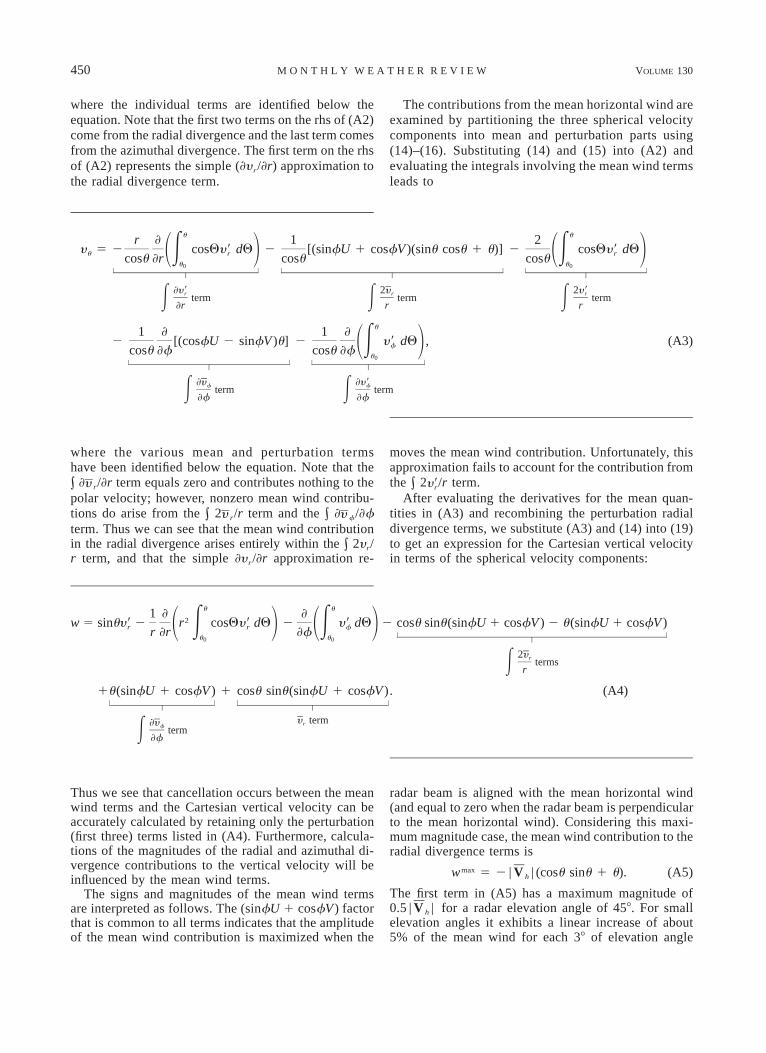
450 VOLUME 130M O N T H L Y W E A T H E R R E V I E W
where the individual terms are identified below theequation. Note that the first two terms on the rhs of (A2)come from the radial divergence and the last term comesfrom the azimuthal divergence. The first term on the rhsof (A2) represents the simple (]y r/]r) approximation tothe radial divergence term.
The contributions from the mean horizontal wind areexamined by partitioning the three spherical velocitycomponents into mean and perturbation parts using(14)–(16). Substituting (14) and (15) into (A2) andevaluating the integrals involving the mean wind termsleads to
u ur ] 1 2y 5 2 cosQy9 dQ 2 [(sinfU 1 cosfV )(sinu cosu 1 u)] 2 cosQy9 dQu E r E r1 2 1 2cosu ]r cosu cosu
u u0 0| | | | | |
z z z
]y9 2y 2y9r r rterm term termE E E]r r r
u1 ] 1 ]2 [(cosfU 2 sinfV )u] 2 y9 dQ ,E f1 2cosu ]f cosu ]f
u0| | | |
z z
(A3)
]y ]y9f fterm termE E]f ]f
where the various mean and perturbation termshave been identified below the equation. Note that the# ] r/]r term equals zero and contributes nothing to theypolar velocity; however, nonzero mean wind contribu-tions do arise from the # 2 r/r term and the # ] f/]fy yterm. Thus we can see that the mean wind contributionin the radial divergence arises entirely within the # 2y r/r term, and that the simple ]y r/]r approximation re-
moves the mean wind contribution. Unfortunately, thisapproximation fails to account for the contribution fromthe # 2 /r term.y9r
After evaluating the derivatives for the mean quan-tities in (A3) and recombining the perturbation radialdivergence terms, we substitute (A3) and (14) into (19)to get an expression for the Cartesian vertical velocityin terms of the spherical velocity components:
u u1 ] ]2w 5 sinuy9 2 r cosQy9 dQ 2 y9 dQ 2 cosu sinu(sinfU 1 cosfV ) 2 u(sinfU 1 cosfV )r E r E f1 2 1 2r ]r ]f | |u u z0 0
2y r termsE r
1u(sinfU 1 cosfV ) 1 cosu sinu(sinfU 1 cosfV ). (A4)| | | |
z z
y termr]yf termE ]f
Thus we see that cancellation occurs between the meanwind terms and the Cartesian vertical velocity can beaccurately calculated by retaining only the perturbation(first three) terms listed in (A4). Furthermore, calcula-tions of the magnitudes of the radial and azimuthal di-vergence contributions to the vertical velocity will beinfluenced by the mean wind terms.
The signs and magnitudes of the mean wind termsare interpreted as follows. The (sinfU 1 cosfV) factorthat is common to all terms indicates that the amplitudeof the mean wind contribution is maximized when the
radar beam is aligned with the mean horizontal wind(and equal to zero when the radar beam is perpendicularto the mean horizontal wind). Considering this maxi-mum magnitude case, the mean wind contribution to theradial divergence terms is
maxw 5 2 | V | (cosu sinu 1 u).h (A5)
The first term in (A5) has a maximum magnitude of0.5 | h | for a radar elevation angle of 458. For smallVelevation angles it exhibits a linear increase of about5% of the mean wind for each 38 of elevation angle
MARCH 2002 451W E Y G A N D T E T A L .
increase. Because this term is offset by the radial pro-jection of the mean wind (a term that is available fromsingle-Doppler observations), it typically is not a prob-lem. The second term in (A5) increases linearly withelevation angle, reaching a maximum of about 1.5 | h |Vas the radar beam approaches vertical. For typical radarelevation angles it has the same dependency as the firstterm; however, it is more significant because the off-setting term from the azimuthal divergence is not avail-able from single-Doppler observations. Thus, if the re-gion sampled by the radar is downwind from the radar,the mean wind radial divergence contribution to the es-timated vertical velocity will be negative (i.e., down-ward motion). Conversely, if the sampled region is up-wind from the radar, the mean wind term will be positive(upward motion).
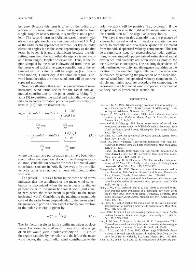
Next, we illustrate that a similar cancellation of meanhorizontal wind terms occurs for the radial and azi-muthal contributions to the polar vorticity. Using (14)and (15) to partition the radial and azimuthal velocitiesinto mean and perturbation parts, the polar vorticity [lastterm in (13)] can be rewritten as
1 1 ]y9rv 5 (cosfU 2 sinfV ) 1u r r cosu ]f| | | |
z z
]y ]y9r rterm term]f ]f
1 1 ](ry 9)f2 (cosfU 2 sinfV ) 2r r ]r
| | | |z z
(A6)
]y ]y9f fterm term]r ]r
where the mean and perturbation terms have been iden-tified below the equation. As with the divergence cal-culation, cancellation between the mean horizontal windcontributions occurs in (A6). If, however, only the radialvelocity terms are retained, a mean wind contributionwill result.
The (cosfU 2 sinfV) factor in the mean wind termsindicates that the amplitude of the mean wind contri-bution is maximized when the radar beam is alignedperpendicular to the mean horizontal wind (and equalto zero when the radar beam is parallel to the meanhorizontal wind). Considering the maximum magnitudecase of the radar beam perpendicular to the mean wind,the mean wind portion of the radial velocity contributionto the polar vorticity is given by
1maxv 5 |V |. (A7)u hr
The 1/r factor results in fairly significant values at closerange. For example, a 20 m s21 mean wind at a rangeof 20 km would yield a polar vorticity of 1023 s21. Ifthe region sampled by the radar is to the left of the meanwind vector, the mean radial wind contribution to the
polar vorticity will be positive (i.e., cyclonic). If thesampled region is to the right of the mean wind vector,the contribution will be negative (anticyclonic).
We have shown in this appendix that the presence ofa mean horizontal wind will introduce a spatial depen-dence to vorticity and divergence quantities estimatedfrom individual spherical velocity components. This canbe a significant issue for meteorological radar applica-tions, where single-Doppler–derived estimates of radialdivergence and vorticity are often used as proxies fortheir Cartesian counterparts. The resulting dependence ofradar-estimated vorticity and divergence quantities on thelocation of the sampled region relative to the radar canbe avoided by removing the projection of the mean hor-izontal wind from the spherical velocity components. Asimple and highly accurate procedure for computing thenecessary mean horizontal wind components from radialvelocity data is presented in section 2b.
REFERENCES
Brewster, K. A., 1984: Kinetic energy evolution in a developing se-vere thunderstorm. M.S. thesis, School of Meteorology, Uni-versity of Oklahoma, Norman, OK, 171 pp.
Burgess, D. W., and L. R. Lemon, 1990: Severe thunderstorm de-tection by radar. Radar in Meteorology, D. Atlas, Ed., Amer.Meteor. Soc., 619–647.
——, and M. A. Magsig, 1998: Recent observations of tornado de-velopment at near range to WSR-88D radars. Preprints, 19thConf. on Severe Local Storms, Minneapolis, MN, Amer. Meteor.Soc., 756–759.
Cressman, G., 1959: An operational objective analysis system. Mon.Wea. Rev., 87, 367–374.
Crook, A., 1994: Numerical experiments initialized with radar-de-rived winds. Part I: Simulated data experiments. Mon. Wea. Rev.,122, 1189–1203.
——, and J. D. Tuttle, 1994: Numerical experiments initialized withradar-derived winds. Part II: Forecasts of three gust front cases.Mon. Wea. Rev., 122, 1204–1217.
Dowell, D. C., and H. B. Bluestein, 1997: The Arcadia, Oklahoma,storm of 17 May 1981: Analysis of a supercell during torna-dogenesis. Mon. Wea. Rev., 125, 2562–2582.
Droegemeier, K. K., 1990: Toward a science of storm-scale predic-tion. Preprints, 16th Conf. on Severe Local Storms, KananaskisPark, Alberta, Canada, Amer. Meteor. Soc., 256–262.
——, 1997: Numerical prediction of thunderstorms: Challenges, po-tential benefits and results from real-time operational tests. WMOBull., 46 (4), 1–13.
Funk, T. W., V. L. DeWald, and Y. J. Lin, 1998: A detailed WSR-88D Doppler radar evaluation of a damaging bow-echo eventon 14 May 1995 over north-central Kentucky. Preprints, 19thConf. on Severe Local Storms, Minneapolis, MN, Amer. Meteor.Soc., 436–439.
Gal-Chen, T., 1978: A method for initializing the anelastic equations:Implications for matching models with observations. Mon. Wea.Rev., 106, 587–606.
——, 1982: Errors in fixed and moving frame of references: Appli-cations for conventional and Doppler radar analysis. J. Atmos.Sci., 39, 2279–2300.
Gao, J., M. Xue, A. Shapiro, Q. Xu, and K. K. Droegemeier, 2001:Three-dimensional simple adjoint velocity retrievals from single-Doppler radar. J. Atmos. Oceanic Technol., 18, 26–38.
Glass, F. H., and M. F. Britt, 2000: Close range WSR-88D obser-vations of several tornadic storms. Preprints, 20th Conf. on Se-vere Local Storms, Orlando, FL, Amer. Meteor. Soc., 190–193.
Hane, C. E., and B. C. Scott, 1978: Temperature and pressure per-

452 VOLUME 130M O N T H L Y W E A T H E R R E V I E W
turbations within convective clouds derived from detailed airmotion information: Preliminary testing. Mon. Wea. Rev., 106,654–661.
Hauser, D., and P. Amayenc, 1986: Retrieval of cloud water and watervapor contents from Doppler radar data in a tropical squall line.J. Atmos. Sci., 43, 823–838.
Hermes, L. G., A. Witt, S. D. Smith, D. Klingle-Wilson, D. Morris,G. J. Stumpf, and M. D. Eilts, 1993: The gust-front detectionand wind-shift detection algorithms for the terminal Dopplerweather radar system. J. Atmos. Oceanic Technol., 10, 693–709.
Klazura, G. E., and D. A. Imy, 1993: A description of the initial setof analysis products available from the NEXRAD WSR-88Dsystem. Bull. Amer. Meteor. Soc., 74, 1293–1311.
Laroche, S., and I. Zawadzki, 1994: A variational analysis methodfor the retrieval of three-dimensional wind field from single-Doppler radar data. J. Atmos. Sci., 51, 2664–2682.
——, and ——, 1995: Retrievals of horizontal winds from single-Doppler clear-air data by methods of cross-correlation and var-iational analysis. J. Atmos. Oceanic Technol., 12, 721–738.
Lazarus, S. M., 1996: The assimilation and prediction of a Floridamulticell storm using single-Doppler data. Ph.D. dissertation,University of Oklahoma, 340 pp.
——, A. Shapiro, and K. Droegemeier, 2001: Application of theZhang–Gal-Chen single-Doppler velocity retrieval to a deep-convective storm. J. Atmos. Sci., 58, 998–1016.
LeDimet, F. X., and O. Talagrand, 1986: Variational algorithms foranalysis and assimilation of meteorological observations: The-oretical aspects. Tellus, 38A, 97–110.
Lemon, L. R., and D. W. Burgess, 1980: Magnitude and implicationsof high speed outflow at severe storm summits. Preprints, 19thConf. on Radar Meteorology, Miami, FL, Amer. Meteor. Soc.,364–368.
Lewis, J., and J. Derber, 1985: The use of adjoint equations to solvea variational problem with advective constraints. Tellus, 37A,309–322.
Lilly, D. K., 1990: Numerical prediction of thunderstorms—Has itstime come? Quart. J. Roy. Meteor. Soc., 116, 779–798.
Lin, Y., P. S. Ray, and K. W. Johnson, 1993: Initialization of a modeledconvective storm using Doppler radar–derived fields. Mon. Wea.Rev., 121, 2757–2775.
Navon, I. M., X. L. Zou, J. Derber, and J. Sela, 1992: Variationaldata assimilation with an adiabatic version of the NMC spectralmodel. Mon. Wea. Rev., 120, 1433–1446.
O’Brien, J. J., 1970: Alternative solutions to the classical verticalvelocity problem. J. Appl. Meteor., 9, 197–203.
Qiu, C. J., and Q. Xu., 1992: A simple adjoint method of wind analysisfor single-Doppler data. J. Atmos. Oceanic Technol., 9, 588–598.
Ray, P. S., B. C. Johnson, K. W. Johnson, J. S. Bradberry, J. J.Stephens, K. K. Wagner, R. B. Wilhelmson, and J. B. Klemp,1981: The morphology of several tornadic storms on 20 May1977. J. Atmos. Sci., 38, 1643–1663.
Rhinehart, R. E., 1979: Internal storm motions from single non-Dopp-ler weather radar. NCAR Tech. Note NCAR/TN-1461STR, 262pp.
Roberts, R. D., and J. W. Wilson, 1989: A proposed microburst now-casting procedure using single-Doppler radar. J. Appl. Meteor.,28, 285–303.
Roux, F., 1985: Retrieval of thermodynamic fields from multipleDoppler radar data using the equations of motion and thermo-dynamic equation. Mon. Wea. Rev., 113, 2142–2157.
Rutledge, S. A., and P. V. Hobbs, 1983: The mesoscale and microscalestructure and organization of clouds and precipitation in a mid-latitude cyclone. VIII: A model for the ‘‘seeder-feeder’’ processin warm-frontal rainbands. J. Atmos. Sci., 40, 1185–1206.
——, and ——, 1984: The mesoscale and microscale structure andorganization of clouds and precipitation in a mid-latitude cy-clone. XII: A diagnostic modeling study of precipitation devel-opment in narrow cold-frontal rainbands. J. Atmos. Sci., 41,2949–2972.
Shapiro, A., and S. Lazarus, 1993: A modified dynamic recoverytechnique for cloud-scale numerical models. Preprints, 17thConf. on Severe Local Storms, St. Louis, MO, Amer. Meteor.Soc., 455–459.
——, S. Ellis, and J. Shaw, 1995a: Single-Doppler velocity retrievalswith Phoenix II data: Clear air and microburst wind retrievalsin the planetary boundary layer. J. Atmos. Sci., 52, 1265–1287.
——, and Coauthors, 1995b: Highlights from a single-Doppler ve-locity retrieval intercomparison project. Preprints, Sixth Conf.on Aviation Weather Systems, Dallas, TX, Amer. Meteor. Soc.,541–546.
Smythe, G. R., and D. S. Zrnic, 1983: Correlation analysis of Dopplerradar data and retrieval of the horizontal wind. J. Climate Appl.Meteor., 22, 297–311.
Sun, J., and A. Crook, 1994: Wind and thermodynamic retrieval fromsingle-Doppler measurements of a gust front observed duringPhoenix II. Mon. Wea. Rev., 122, 1075–1091.
——, and ——, 1996: Comparison of thermodynamic retrieval bythe adjoint method with the traditional retrieval method. Mon.Wea. Rev., 124, 308–324.
——, and ——, 1997: Dynamic and microphysical retrieval fromDoppler radar observations using a cloud model and its adjoint.Part I: Model development and simulated data experiments. J.Atmos. Sci., 54, 1642–1661.
——, and ——, 1998: Dynamic and microphysical retrieval fromDoppler radar observations using a cloud model and its adjoint.Part II: Retrieval experiments of an observed Florida convectivestorm. J. Atmos. Sci., 55, 835–852.
——, D. W. Flicker, and D. K. Lilly, 1991: Recovery of three-di-mensional wind and temperature fields from simulated single-Doppler radar data. J. Atmos. Sci., 48, 876–890.
Talagrand, O., and P. Courtier, 1987: Variational assimilation of me-teorological observations with the adjoint vorticity equations.Part I: Theory. Quart. J. Roy. Meteor. Soc., 113, 1311–1328.
Taylor, G. I., 1938: The spectrum of turbulence. Proc. Roy. Soc.London, A164, 476–490.
Thepaut, J., D. Vasiljevic, and P. Coutier, 1993: Variational assimi-lation of conventional meteorological observations with a mul-tilevel primitive equation model. Quart. J. Roy. Meteor. Soc.,119, 153–186.
Trapp, R. J., and C. A. Doswell, 2000: Radar data objective analysis.J. Atmos. Oceanic Technol., 17, 105–120.
Tuttle, J. D., and G. B. Foote, 1990: Determination of the boundarylayer airflow from a single Doppler radar. J. Atmos. OceanicTechnol., 7, 218–232.
Uyeda, H., and D. S. Zrnic, 1986: Automatic detection of gust fronts.J. Atmos. Oceanic Technol., 3, 36–50.
Verlinde, J., and W. R. Cotton 1990: A critical look at microphysicalretrieval algorithms. Preprints, Conf. on Cloud Physics, SanFrancisco, CA, Amer. Meteor. Soc., 453–457.
——, and ——, 1993: Fitting microphysical observations of non-steady convective clouds to a numerical model: An applicationof the adjoint technique of data assimilation to a kinematic mod-el. Mon. Wea. Rev., 121, 2776–2793.
Weygandt, S. S., A. Shapiro, and K. K. Droegemeier, 2002: Retrievalof model initial fields from single-Doppler observations of asupercell thunderstorm. Part II: Thermodynamic Retrieval andnumerical prediction. Mon. Wea. Rev., 130, 454–476.
Wilson, J. W., R. D. Roberts, C. Kessinger, and J. McCarthy, 1984:Microburst wind structure and evaluation of Doppler radar forairport wind shear detection. J. Appl. Meteor., 23, 898–915.
——, N. A. Crook, C. K. Mueller, J. Sun, and M. Dixon, 1998:Nowcasting thunderstorms: A status report. Bull. Amer. Meteor.Soc., 79, 2079–2099.
Witt, A., and S. P. Nelson, 1984: The relationship between upper-level divergent outflow magnitude as measured by Doppler radarand hailstorm intensity. Preprints, 22nd Conf. on Radar Mete-orology, Zurich, Switzerland, Amer. Meteor. Soc., 108–111.
Xu, Q., 1996: Generalized adjoint for physical processes with pa-

MARCH 2002 453W E Y G A N D T E T A L .
rameterized discontinuities. Part I: Basic issues and heuristicexamples. J. Atmos. Sci., 53, 1123–1142.
Xu, Q., C. J. Qiu, and J. X. Yu, 1994a: Adjoint method retrievals oflow-altitude wind fields from single-Doppler reflectivity mea-sured during Phoenix-II. J. Atmos. Oceanic Technol., 11, 275–288.
——, ——, ——, 1994b: Adjoint method retrievals of low-altitudewind fields from single-Doppler wind data. J. Atmos. OceanicTechnol., 11, 579–585.
——, ——, H. D. Gu, and J. X. Yu, 1995: Simple adjoint retrievalsof microburst winds from single-Doppler data. Mon. Wea. Rev.,123, 1822–1833.
——, H. D. Gu, and S. Yang, 2001: Simple adjoint method for three-dimensional wind retrievals from single-Doppler data. Quart. J.Roy. Meteor. Soc., 127, 1053–1067.
Xue, M., K. K. Droegemeier, and V. Wong, 2000: The AdvancedRegional Prediction System (ARPS)—A multiscale nonhydros-tatic atmospheric simulation and prediction tool. Part I: Modeldynamics and verification. Meteor. Atmos. Phys., 75, 161–193.
——, and Coauthors, 2001: The Advanced Regional Prediction Sys-
tem (ARPS)—A multiscale nonhydrostatic atmospheric simu-lation and prediction tool. Part II: Model physics and applica-tions. Meteor. Atmos. Phys., 75, 161–193.
——, ——, ——, A. Shapiro, and K. Brewster, 1995: ARPS User’sGuide, Version 4.0., Center for Analysis and Prediction ofStorms, 380 pp.
Zhang, J., and T. Gal-Chen, 1996: Single-Doppler wind retrieval inthe moving frame of reference. J. Atmos. Sci., 53, 2609–2623.
Ziegler, C. L., 1985: Retrieval of thermal and microphysical variablesin observed convective storms. Part I: Model development andpreliminary testing. J. Atmos. Sci., 42, 1487–1509.
——, 1988: Retrieval of thermal and microphysical variables in ob-served convective storms. Part II: Sensitivity of cloud processesto variation of the microphysical parameterization. J. Atmos. Sci.,45, 1072–1090.
Zou, X. L., I. M. Navon, and J. Sela, 1993: Variational data assim-ilation with threshold processes using the NMC multilevel prim-itive-equation model. Tellus, 45A, 370–387.
Zupanski, M., 1993: Regional four-dimensional variational data as-similation in a quasi-operational forecasting environment. Mon.Wea. Rev., 121, 2396–2408.