Embed Size (px)
Citation preview
Retrieval of Atmospheric Ozone Concentrations from Satellite Based Limb Data
Sheng Bo Chen
College of Geoexploration Science and Technology, Jilin [email protected]

Outline
1. Introduction2. SCHIMACHY Data3. Inversion Method4. Inversion Error Analysis5. Inversion Validation6. Conclusions

1. Introduction
Atmospheric Sounding experienced ground-based detection, balloon soundings and rockets and other space technology , since the satellite- based atmospheric sounding instruments there.
Ground-based Measurement
Invented in 1924 Dobson detector
1973 Brewer foundation VIS spectrometer NO2
Balloon Soundings
Detect height 30-35 km
1988 McElroy limb spectrometer NO2
Plane and Rockets
70 s the stratosphere and interface layer
Satellite-based Measurement
Worldwide

Satellite Measurement
Observatory Geometry
Nadir Measurements
Occultation Measurements
Limb Measurements
-72 -70 -68 -66 -64 -62 -60 -5836
37
38
39
40
41
42
43
44
45

Limb Based Instruments
Limb Measurements
1973 Cunnold step one proposed limb scattering techniques, used in aircraft. Wavelength UV-VIS 6.
2010 CAS Changchun Institute of Optics, limb imaging spectrometer prototype. UV 270-390 nm and VIS 540-780 nm
Instruments Aircraft Launch time Main science mission
UVS SME 1981.10.6 Study the Earth's upper atmosphere ozone production and loss processes
SOLSE/LORE STS-87 1997.10 Experiment with limb scattering observations of ozone profile technology
OSIRIS Odin 2001.2.20 Identify the number density of important trace atmospheric constituents, such as O3 ,NO2 ,OClO and BrO Etc
SAGE Ⅲ Meteor3M/ISS 2001.12.10/2004 Provide long-term global atmospheric important composition and temperature observations
SCIAMACHY ENVISAT 2002.3.1 Detecting the concentration and distribution of atmospheric composition and surface phenomena
OMPS NPOESS Plan 2013 Detect the total amount and vertical distribution of O3 ,NO2 ,OClO,HCHO and SO2.
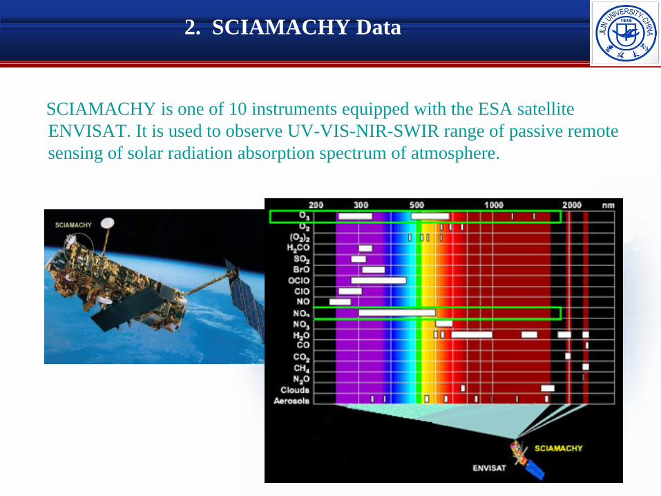
2. SCIAMACHY Data
SCIAMACHY is one of 10 instruments equipped with the ESA satellite ENVISAT. It is used to observe UV-VIS-NIR-SWIR range of passive remote sensing of solar radiation absorption spectrum of atmosphere.

SCIAMACHY is designed to a double imager and divided into eight channels, the instrument records the reflection and scattering of solar radiation spectrum range through 214-2386 nm wavelength, with moderate spectral resolution 0.24-1.48 nm.

< 1000 nm, 2350 nm
Select data:Determine the wavelength
200 300 400 500 600 700 800 900 1000 11000
5
10
15
20
25
212.5855 213.1905 (1)213.3414 239.9363 (2)
240.0656 281.923 (3)282.0343 313.939 (4)
314.05 333.821 (5)333.9349 334.3908 (6)
411.7432 412.1773 (7)404.0723 411.6347 (8)
320.1644 403.9647 (9)309.4543 320.0517 (10)
301.1927 309.339 (11)300.6049 301.0752 (12)
383.517 385.7903 (13)386.0426 391.5754 (14)391.8261 605.4468 (15)
605.6889 627.1788 (16)627.4251 628.4114 (17)
595.3128 596.2095 (18)596.4335 597.3292 (19)597.5531 789.8091 (20)
790.0212 811.2286 (21)811.4452 812.3121 (22)
773.192 774.4019 (23)774.704 775.9122 (24)776.214 1056.1941(25)
Wavelength(nm)
Clu
ster
ID
SCIAMACHY L1C Cluster Spectrum Band
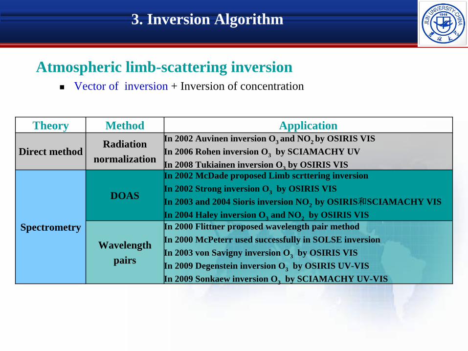
3. Inversion Algorithm
Atmospheric limb-scattering inversion
Vector of inversion + Inversion of concentration
Theory Method Application
Direct methodRadiation
normalization
In 2002 Auvinen inversion O3 and NO2 by OSIRIS VISIn 2006 Rohen inversion O3 by SCIAMACHY UVIn 2008 Tukiainen inversion O3 by OSIRIS VIS
Spectrometry
DOAS
In 2002 McDade proposed Limb scrttering inversionIn 2002 Strong inversion O3 by OSIRIS VISIn 2003 and 2004 Sioris inversion NO2 by OSIRIS和SCIAMACHY VISIn 2004 Haley inversion O3 and NO2 by OSIRIS VIS
Wavelengthpairs
In 2000 Flittner proposed wavelength pair methodIn 2000 McPeterr used successfully in SOLSE inversionIn 2003 von Savigny inversion O3 by OSIRIS VISIn 2009 Degenstein inversion O3 by OSIRIS UV-VISIn 2009 Sonkaew inversion O3 by SCIAMACHY UV-VIS
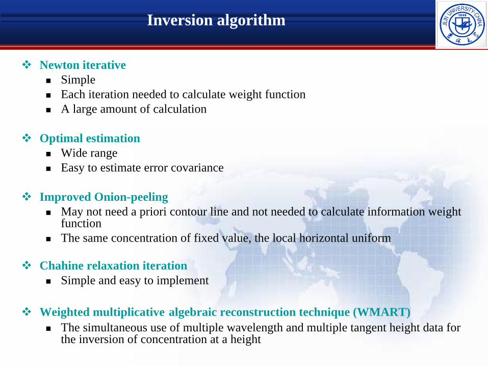
Inversion algorithm
Newton iterative
Simple
Each iteration needed to calculate weight function
A large amount of calculation
Optimal estimation
Wide range
Easy to estimate error covariance
Improved Onion-peeling
May not need a priori contour line and not needed to calculate information weight function
The same concentration of fixed value, the local horizontal uniform
Chahine relaxation iteration
Simple and easy to implement
Weighted multiplicative algebraic reconstruction technique (WMART)
The simultaneous use of multiple wavelength and multiple tangent height data for the inversion of concentration at a height

According to the meteorological data assuming an initial target of ozone profiles, using SCIATRAN model to simulate the limb radiation and compared with SCIAMACHY satellite radiation.The radiation difference value is feedback information to adjusting the ozone profile. Then we use this profile simulation new radiation value in order to better to match the observed value iteration processing.The result is the ozone profile.
Weighted multiplicative algebraic reconstruction inversion method (WMART)
wavelength Inversion target Inversion method
Hartley and Chappuis
ozone vertical profile
Wavelength pairs +Weighted multiplicative algebraic reconstruction
UV-VIS Limb data
Radiation normalization
Wavelength pairs
Weighted multiplicative algebraic reconstruction SCIATRAN
Ozone profile
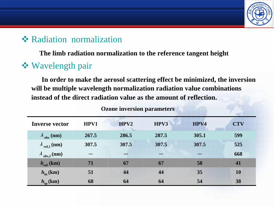
Radiation normalizationThe limb radiation normalization to the reference tangent height
Wavelength pairIn order to make the aerosol scattering effect be minimized, the inversion
will be multiple wavelength normalization radiation value combinations instead of the direct radiation value as the amount of reflection.
Ozone inversion parameters
Inverse vector HPV1 HPV2 HPV3 HPV4 CTV
λobs (nm) 267.5 286.5 287.5 305.1 599
λref,1 (nm) 307.5 307.5 307.5 307.5 525
λobs,2 (nm) - - - - 668
href (km) 71 67 67 58 41
hbt (km) 51 44 44 35 10
htp (km) 68 64 64 54 38

Wavelength pairs effect
0 2 4 6 8
x 1013
0
10
20
30
40
50
60
λ = 525 nm
0 1 2 3 4 5
x 1013
0
10
20
30
40
50
60
Tang
ent a
ltitu
de (k
m)
λ = 599 nm
0 50 100 150 2000
10
20
30
40
50
60
Normalized radiance
λ = 668 nm
0 20 40 60 80 1000
10
20
30
40
50
60
λ = 525 nm
0 20 40 60 80 1000
10
20
30
40
50
60
λ = 599 nm
0 2 4 6
x 1013
0
10
20
30
40
50
60
Radiance (photons s-1 cm-2 nm-1 sr-1)
λ = 668 nm
A=0.0A=0.2
A=0.4
A=0.6
A=0.8A=1.0
A=0.0A=0.2
A=0.4
A=0.6
A=0.8A=1.0
A=0.0
A=0.2
A=0.4A=0.6
A=0.8
A=1.0
A=0.0A=0.2
A=0.4
A=0.6
A=0.8A=1.0
A=0.0
A=0.2
A=0.4A=0.6
A=0.8
A=1.0
A=0.0A=0.2
A=0.4
A=0.6
A=0.8A=1.0
Tang
ent a
ltitu
de (k
m)
cloud Surface albedo
aerosol

Aerosol sensitivity
= 267.5 nm
0 0035 0 004
0.004
0.00450 005 0 0055
0.006
0.00650.007
Tang
ent a
ltitud
e (k
m)
30 40 50 60 70 80 90
55
60
65
= 286.5 nm0.004
0.0040.004
0.005
0.005
0.0050.006
0.006
0.007
0.0070.0080.009
30 40 50 60 70 80 9045
50
55
60
= 305.1 nm0.004
0 0040.004
0.005
0 005
0.005
0.006
0 006
0.006 0.007
0.007
0.008
0.0080.0090.01
Solar zenith angle (°)
Tang
ent a
ltitud
e (k
m)
30 40 50 60 70 80 9035
40
45
50
= 599.0 nm-0.05
-0.05-0.05
0
00
0.05
0.050.05
0.1
0.10.1
0.15
0.15
0.2
0.20.2
0.25
0.250.25
0.3
0.2
Solar zenith angle (°)30 40 50 60 70 80 90
15
20
25
30
35
HPV1
-0 0035-0 003-0 0025-0 002-0.0015-0.001-0.0005
00
0.0005
0.0005
Tang
ent a
ltitud
e (k
m)
30 40 50 60 70 80 90
55
60
65
HPV20.0045
-0.0045
0.004
-0.004-0.004
0.0035
-0.0035
0.003
-0.003
0.0025
-0.0025
0.002
-0.002
0.0015
-0.0015
0.001
-0.001
0.0005
-0.0005
0
00
30 40 50 60 70 80 9045
50
55
60
0.0006
-0.00060 0006
0.0005
-0.0005
0 0005
0.0004
-0.0004
0.0003
-0.0003
0.0002
-0.0002
0.0001-0.0001
Solar zenith angle (°)
Tang
ent a
ltitud
e (k
m)
HPV3
30 40 50 60 70 80 9035
40
45
50
CTV-0.07
-0.07-0.07
-0.06
-0.06-0.06
-0.05
-0.05-0.05
-0.04
-0.04-0.04
-0.03
-0.03-0.03
-0.02
-0.02-0.02
Solar zenith angle (°)30 40 50 60 70 80 90
15
20
25
30
35
The radiation relative deviation under the influence of aerosol
The inversion vector relative deviation under the influence of aerosol
1. Before processing: Hartley band along with the change of SZA ↑↑;Chappuis band is insensitive to SZA, but depend on TH and in 21 km reach the maximum peak.
2. After processing: Two bands are not sensitive to SZA and along with rising TH reduced↑↓.0 influence lines, negative influence

Cloud sensitivity
= 305.1 nme 005
2e-005
2e-005
e 005
4e-005
4 005
6e 005
6e-005
6 005
8e 005
8e-005
8 005
0.0001
0 0001
0.00012
0 00012
0.00014
0.00014
Solar zenith angle (°)
Tang
ent a
ltitud
e (k
m)
30 40 50 60 70 80 9035
40
45
50
= 599.0 nm
00
0
0
0 0
0.01
0.01
0.01 0.01 0.02
0.02
0.02
0.02
0.02
0.02
0.03
0.030.03
0.03
0.03
0.04
0.04
0.04
0.04
0.04
0.05
0.05
0.05
0.05
0.06
0.06
0.06
0.06
0.07
0.07
0.08
Solar zenith angle (°)30 40 50 60 70 80 90
15
20
25
30
35
HPV1
-2e-005
-2e-005
-1 5e-005
-1.5e-005
-1.5e-005
-1e-005-1e-005
5e 006
Tang
ent a
ltitud
e (k
m)
30 40 50 60 70 80 90
55
60
65
HPV21.8e 005 1.8e 005
-1.8e-005
1.6e 005 1.6e 005
-1.6e-005
1.4e 005 1.4e 005
-1.4e-005
1.2e 005 1.2e 005
-1.2e-005
-1.2e-005
-1.2e-005-1.2e-005
1e 005
-1e-005
-1e-005
-1e-005
8e 006
-8e-006
-8e-006
6e 006
-6e-006
-6e-006-6e-006
4e 006
-4e-006
-4e-006-4e-006
2e 006-2e-006
-2e-006
-1.2e-005
-1.4e-005
-1e-005
00 0
-8e-00630 40 50 60 70 80 90
45
50
55
60
HPV45e 006 5e 006
5e 0065e 006
0
00
-5e-006
-5e-006
5e-006
5e 006
1e-005
1 5e 005
0
Solar zenith angle (°)
Tang
ent a
ltitud
e (k
m)
30 40 50 60 70 80 9035
40
45
50
HPV4-0.04 -0.04
-0.04-0.04
-0.035 -0.035
-0.035-0.035
-0.03 -0.03
-0.03-0.03
-0.025 -0.025
-0.025-0.025
-0.02 -0.02
-0.02
-0.02
-0.015 -0.015
-0.015
-0.015
-0.01-0.01
-0.01
-0.01
-0.005 -0.005
-0.005
0
0
0
Solar zenith angle (°)30 40 50 60 70 80 90
15
20
25
30
35
The radiation value relative deviationunder the influence of cloud
The inversion vector relative deviation under the influence of cloud
1. Before processing : <300 nm no effect ,SZA ↑↓
2. After processing :TH ↑↓, negative effect; HPV negative peak around SZA 60,CTV Negative peak in SZA 80

Surface albedo sensitivity
= 305.1 nm0 0005
0.0005
0.00050 0005
0 00
0.001
0.001
0 001
0.0015
0.0015
0 0015
0 00
0.002
0 002
0.0025
0 0025
0.003
0 003
0.0035
0.0035.004
Solar zenith angle (°)
Tang
ent a
ltitud
e (k
m)
30 40 50 60 70 80 9035
40
45
50
= 599.0 nm0.05 0.05
0.05
0.050.050.05
0.1 0.1
0.1
0.1
0.10.1
0.150.15
0.15
0.150.15
0.2
0.2
0.20.2
0.25
Solar zenith angle (°)30 40 50 60 70 80 90
15
20
25
30
35
HPV15e 005 5e-005
5e-005
0 000
0.0001
0 0001
0.00015
0.000150 00015
0.0002
0.0002
0 0002
0.00025
0 00025
0.0003
0 0003
0.000350.0004
0.00045
Tang
ent a
ltitud
e (k
m)
30 40 50 60 70 80 90
55
60
65
HPV20 0
00
5e-005
5e-005
5e-0055e-005
0.0001
0.00010.0001
0.00015
0.00015
0.00015
0.0002
0.0002
0.00025
0.000250.0003
0.0003
0.00035
30 40 50 60 70 80 9045
50
55
60
HPV40.00035 0.00035
0 000350 00035
0.0003 0.0003
0 00030 0003
0.00025 0.00025
0 00025-0.00025
0.0002 0.0002
0 0002-0.0002
0.00015 0.00015
0 00015
-0.00015
0.0001 0.0001
0 0001
-0.0001
5e 005 5e 005
5e 005
-5e-005
0 0
00
0
5e 0055e-005
5e-005
5e-005
0.0001
0.0001
Solar zenith angle (°)
Tang
ent a
ltitud
e (k
m)
30 40 50 60 70 80 9035
40
45
50
CTV0.005 0.005
0.0050.005
0.01
0.01
0.010.01
0.015
0.015
0.0150.015
0.02
0.02
0.020.02
0.0250.025
0.025
0.03
0.030.03
0.035
0.0350.035
0.04
0.040.040.045
0.0450.045 0.050.050.055
Solar zenith angle (°)30 40 50 60 70 80 90
15
20
25
30
35
The radiation relative deviation under the influence of surface albedo without processing
The inversion vector relative deviation under the influence of surface albedo
1. Before processing :SZA↑↓2. After processing :HPV with SZA↑↓ , dependent on TH;
CTV along with rising SZA and TH reduced ↑↓

Sensitivity summary
Before processing After processing
wavelength Three factors increase with wavelength increaseing; Chappuis
band >Hartley bandChappuis band >Hartley band
SZA The three factors are dependent on the SZA
The three factor is not entirely dependent on the SZA
After processing:The influence of three factors are reduced to a lower magnitude
The influence degree of the value of radiationAerosol> cloud > surface albedo

WMART
A number of bands and tangent radiation
obs
modkj
ki jij kj
yW
y
obs,( 1) ( )
modk jn n
i i ki jik j kj
yx x W W
y
tangent height
bands
i – inversion height,k – Wavelength combination,j – tangent height radiation
step1 Band correction factor
step2 Height correction factor
step3 Density correction
i ki kik
W
( 1) ( )n ni i ix x

Band combination weight factors
Ozone weight factors
Weight function has a different range and has different combinations at different height.
Smooth
Start 0 ,end 0
0 0.5 10
10
20
30
40
50
60
70
Weighting Factor
Tang
ent A
ltitu
de (k
m)
HPV1HPV2HPV3HPV4CTV

Inversion Implementation
SCIATRAN
SCIAMACHY L1B
SCIAMACHY L1C
Calibrate
Extract
Observed radiance
Radiance normalization
Wavelength pairing
Observed vector
Annotation parameters
Model radiance by SCIATRAN
Modeled vector
Retrieve by WMART
Input tracegas profiles
Modeled radiance
Trace gas profiles
Meet condition
Yes
End
No
SCIA_JLUAutomatic batch processing multi-track SCIAMACHY dataO3 (30 min/26prf)and NO2(15min/104prf)
4. Inversion Error Analysis
The main error source
Tangent positioning
AerosolBoundary layer visibilityStratospheric aerosol loadExtinction coefficient
Surface albedo
Cloud parametersCloud heightCloud optical thickness
Analysis method
Parameters deviation,SCIATRAN

4.1 Tangent height positioning error
Ozone inversion error
-30 -20 -10 0 10 20 30 4010
30
50
70
Relative percent error (%)
Altit
ude
(km
)
(1) SZA = 30° TH=[0.25-1.00]
-30 -20 -10 0 10 20 30 4010
30
50
70
Relative percent error (%)
(2) SZA = 40° TH=[0.25-1.00]
-30 -20 -10 0 10 20 30 4010
30
50
70
Relative percent error (%)
(3) SZA = 50° TH=[0.25-1.00]
-30 -10 10 30 5010
30
50
70
Relative percent error (%)
Altit
ude
(km
)
(4) SZA = 60° TH=[0.25-1.00]
-20 -10 0 10 20 30 40 5010
30
50
70
Relative percent error (%)
(5) SZA = 70° TH=[0.25-1.00]
-20 0 20 4010
30
50
70
Relative percent error (%)
(6) SZA = 80° TH=[0.25-1.00]
-20 -10 0 10 20 3010
30
50
70
Relative percent error (%)
Altit
ude
(km
)
(7) SZA = 90° TH=[0.25-1.00]
-10 -5 0 5 10 1510
30
50
70
Relative percent error (%)
(8) SZA = [30-90]° TH=0.25
TH0.25TH0.50TH1.00
SZA30SZA40SZA50SZA60SZA70SZA80SZA90
subplot (1) - (7) subplot (8)
dTH∈{0.25, 0.5, 1} km
dTH↑error↑,0.25 km (10 %)
positive and negative,58 km maximum error
SZA haveLittle effect,SZA=70 maximum error
Altit
ude
(km
)
(1) SZA - H
30 40 50 60 70 80 9010
20
30
40
50
60
70
Tang
ent a
ltitud
e bi
as
(2) H = 20 km
30 40 50 60 70 80 900.25
0.50
1.00
Solar zenith angle (°)
Tang
ent a
ltitud
e bi
as(3) H = 40 km
30 40 50 60 70 80 900.25
0.50
1.00
Solar zenith angle (°)
Tang
ent a
ltitud
e bi
as
(4) H = 60 km
30 40 50 60 70 80 900.25
0.50
1.00
-5
0
5
10
-20
-15
-10
-5
2
4
6
8
5
10
15
20
25
30
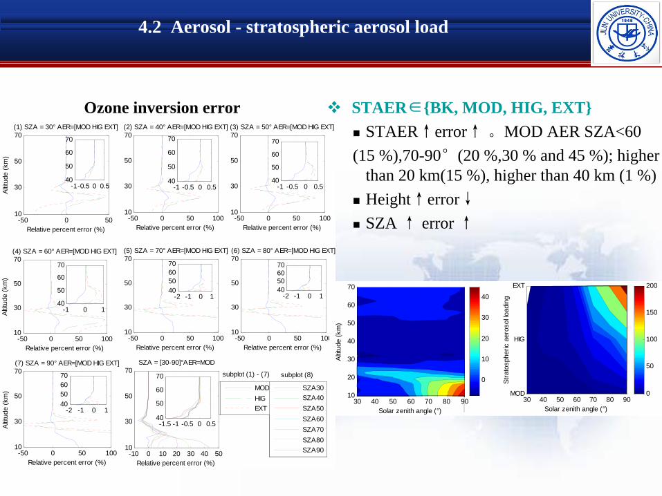
4.2 Aerosol - stratospheric aerosol load
Ozone inversion error
-50 0 5010
30
50
70(1) SZA = 30° AER=[MOD HIG EXT]
Relative percent error (%)
Altit
ude
(km
)
-50 0 50 10010
30
50
70(2) SZA = 40° AER=[MOD HIG EXT]
Relative percent error (%)-50 0 50 100
10
30
50
70(3) SZA = 50° AER=[MOD HIG EXT]
Relative percent error (%)
-50 0 50 10010
30
50
70(4) SZA = 60° AER=[MOD HIG EXT]
Relative percent error (%)
Altit
ude
(km
)
-50 0 50 10010
30
50
70(6) SZA = 80° AER=[MOD HIG EXT]
Relative percent error (%)
-50 0 50 10010
30
50
70(7) SZA = 90° AER=[MOD HIG EXT]
Relative percent error (%)
Altit
ude
(km
)
MODHIGEXT
-50 0 50 10010
30
50
70(5) SZA = 70° AER=[MOD HIG EXT]
Relative percent error (%)
-10 0 10 20 30 40 5010
30
50
70SZA = [30-90]°AER=MOD
Relative percent error (%)
SZA30SZA40SZA50SZA60SZA70SZA80SZA90
-1-0.5 0 0.540
50
60
70
-1 -0.5 0 0.540
50
60
70
-1 -0.5 0 0.540
50
60
70
-1 0 140
50
60
70
-2 -1 0 140506070
-2 -1 0 140506070
-2 -1 0 140506070
MODHIGEXT
-1.5 -1 -0.5 0 0.540
50
60
70
SZA30SZA40SZA50SZA60SZA70SZA80SZA90
subplot (8)subplot (1) - (7)
STAER∈{BK, MOD, HIG, EXT}
STAER↑error↑。MOD AER SZA<60 (15 %),70-90°(20 %,30 % and 45 %); higher
than 20 km(15 %), higher than 40 km (1 %)
Height↑error↓
SZA ↑ error ↑
Solar zenith angle (°)
Altit
ude
(km
)
30 40 50 60 70 80 9010
20
30
40
50
60
70
0
10
20
30
40
Solar zenith angle (°)
Stra
tosp
heric
aer
osol
load
ing
30 40 50 60 70 80 90MOD
HIG
EXT
0
50
100
150
200

4.3 Aerosol-extinction coefficient
Ozone inversion error
-10 0 10 2010
30
50
70(1) SZA = 30° AER=[2-4]
Relative percent error (%)
Altit
ude
(km
)
-20 0 20 4010
30
50
70(2) SZA = 40° AER=[2-4]
Relative percent error (%)-20 0 20 40
10
30
50
70(3) SZA = 50° AER=[2-4]
Relative percent error (%)
-20 0 20 4010
30
50
70(4) SZA = 60° AER=[2-4]
Relative percent error (%)
Altit
ude
(km
)
-20 0 20 4010
30
50
70(5) SZA = 70° AER=[2-4]
Relative percent error (%)-20 0 20 40
10
30
50
70(6) SZA = 80° AER=[2-4]
Relative percent error (%)
-20 0 20 4010
30
50
70(7) SZA = 90° AER=[2-4]
Relative percent error (%)
Altit
ude
(km
)
-10 0 10 2010
30
50
70(8) SZA = [30-90]° dAER=1
Relative percent error (%)
AER2AER3AER4
SZA30SZA40SZA50SZA60SZA70SZA80SZA90
subplot (1) - (7) subplot (8)
Multiple∈{2, 3, 4}●
Multiple↑error↑●
2 times ,10-68 km(12 %);higher than 22 km (5 %)●
Height↑error first↑ then↓●
SZA ↑error↑
Solar zenith angle (°)
Altit
ude
(km
)
30 40 50 60 70 80 9010
20
30
40
50
60
70
Solar zenith angle (°)
Aero
sol s
calin
g pa
ram
eter
30 40 50 60 70 80 902
3
4
4
6
8
10
12
14
16
18
0
5
10

4.4 Surface albedo
Ozone inversion error
-15 -10 -5 0 5 10 1510
30
50
70
Altit
ude
(km
)
(1) SZA = 30° ALB=[0.0-1.0]
-15 -10 -5 0 5 10 1510
30
50
70(2) SZA = 40° ALB=[0.0-1.0]
-15 -10 -5 0 5 10 1510
30
50
70
Altit
ude
(km
)
(3) SZA = 50° ALB=[0.0-1.0]
-10 -5 0 5 1010
30
50
70(4) SZA = 60° ALB=[0.0-1.0]
-5 -3 -1 1 3 510
30
50
70
Altit
ude
(km
)
(5) SZA = 70° ALB=[0.0-1.0]
-4 -2 0 2 410
30
50
70(6) SZA = 80° ALB=[0.0-1.0]
-2 -1 0 1 210
30
50
70
Relative percent error (%)
Altit
ude
(km
)
(7) SZA = 90° ALB=[0.0-1.0]
-3 -2 -1 0 1 2 310
30
50
70
Relative percent error (%)
(8) SZA = [30-90]° dALB=±0.1
ALB0.0ALB0.1ALB0.2ALB0.3ALB0.4ALB0.6ALB0.7ALB0.8ALB0.9ALB1.0
SZA30SZA40SZA50SZA60SZA70SZA80SZA90SZA30SZA40SZA50SZA60SZA70SZA80SZA90
solid line: dALB = -0.1dot line: dALB = 0.1
subplot (1) - (7)
subplot (8)
ALB∈{0, 0.1, 0.2, 0.3, 0.4, 0.5, 0.6, 0.7, 0.8, 0.9, 1}
dALB↑error↑,Symmetric distribution
dALB=0.1,35-68 km(0.5 %), under 35 km (3 %)
height↑error↓
SZA ↑error↓
Solar zenith angle (°)
Altit
ude
(km
)
30 40 50 60 70 80 9010
20
30
40
50
60
70
Solar zenith angle (°)
Albe
do
30 40 50 60 70 80 900.0
0.1
0.2
0.3
0.4
0.6
0.7
0.8
0.9
1.0
0
0.5
1
1.5
2
-10
-5
0
5
10

4.5 Cloud height
Ozone inversion error
CLD∈{[2.4-3], [0.6-3], [0.3-1], [5- 10], [8-15]} km
Troposphere cloud small( within 2 %); stratosphere cloud error is the largest (50 %)
height ↑error↓
Insensitive to SZA
-0.2 0 0.2 0.4 0.6 0.810
30
50
70
Relative percent error (%)
Altit
ude
(km
)
-0.2 0 0.2 0.4 0.6 0.810
30
50
70
Relative percent error (%)
-0.5 0 0.5 110
30
50
70
Relative percent error (%)
Altit
ude
(km
)
-0.5 0 0.5 1 1.510
30
50
70
Relative percent error (%)
-0.5 0 0.5 1 1.5
20
40
60
Relative percent error (%)
Altit
ude
(km
)
-0.5 0 0.5 1 1.5 210
30
50
70
Relative percent error (%)
-0.5 0 0.5 1 1.510
30
50
70
Relative percent error (%)
Altit
ude
(km
)
Solar zenith angle (°)
30 40 50 60 70 80 9010
30
50
70
0
0.5
1
ASCUST
ASCUST
ASCUST
ASCUST
ASCUST
ASCUST
ASCUST
(4) SZA = 60°(3) SZA = 50°
(1) SZA = 30° (2) SZA = 40°
(5) SZA = 70° (6) SZA = 80°
(7) SZA = 90° (8) AS

4.6 Cloud optical thickness
Ozone inversion error
-1 0 1 2 3 410
30
50
70(1) SZA = 30° tau=[0.05-3]
Relative percent error (%)
Altit
ude
(km
)
-1 0 1 2 310
30
50
70(2) SZA = 40° tau=[0.05-3]
Relative percent error (%)
-1 0 1 2 3 410
30
50
70(3) SZA = 50° tau=[0.05-3]
Relative percent error (%)
-1 0 1 2 3 410
30
50
70(4) SZA = 60° tau=[0.05-3]
Relative percent error (%)
Altit
ude
(km
)
-1 0 1 2 3 410
30
50
70(5) SZA = 70° tau=[0.05-3]
Relative percent error (%)
-1 0 1 2 3 410
30
50
70(6) SZA = 80° tau=[0.05-3]
Relative percent error (%)
-1 0 1 2 310
30
50
70(7) SZA = 90° tau=[0.05-3]
Relative percent error (%)
Altit
ude
(km
)
-0.1 0.1 0.3 0.5 0.7 0.9 1.110
30
50
70(8)SZA = [30-90]° tau=0.05
Relative percent error (%)
tau0.05tau2tau3
SZA30SZA40SZA50SZA60SZA70SZA80SZA90
-0.1 0 0.140
50
60
70
-0.2-0.1 0 0.140
50
60
70
-0.1 0.150
60
70
SZA30SZA40SZA50SZA60SZA70SZA80SZA90
-0.1 0 0.1 0.240
50
6070
-0.1 0 0.1 0.240
506070
0 0.2 0.440
50
60
70
-0.1 0 0.1 0.240
50
6070
-0.2 -0.1 040
50
60
70
subplot (1) - (7) subplot (8)
TAU∈{0.05, 1, 2, 3}
dTAU↑error↑4 %, higher than 40 km (0.4 %)
height ↑error↓
SZA ↑error first ↑ then ↓
Solar zenith angle (°)
Altit
ude
(km
)
30 40 50 60 70 80 9010
20
30
40
50
60
70
Solar zenith angle (°)
Clo
ud o
ptic
al d
epth
30 40 50 60 70 80 900.05
2
3
5
10
15
20
25
0
0.2
0.4
0.6
0.8
1
1.2
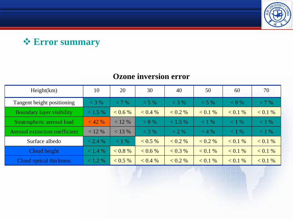
Error summary
Height(km) 10 20 30 40 50 60 70
Tangent height positioning < 3 % < 7 % < 5 % < 3 % < 5 % < 8 % < 7 %
Boundary layer visibility < 1.5 % < 0.6 % < 0.4 % < 0.2 % < 0.1 % < 0.1 % < 0.1 %
Stratospheric aerosol load < 42 % < 12 % < 8 % < 1.5 % < 1 % < 1 % < 1 %
Aerosol extinction coefficient < 12 % < 13 % < 3 % < 2 % < 4 % < 1 % < 1 %
Surface albedo < 2.4 % < 1 % < 0.5 % < 0.2 % < 0.2 % < 0.1 % < 0.1 %
Cloud height < 1.4 % < 0.8 % < 0.6 % < 0.3 % < 0.1 % < 0.1 % < 0.1 %
Cloud optical thickness < 1.2 % < 0.5 % < 0.4 % < 0.2 % < 0.1 % < 0.1 % < 0.1 %
Ozone inversion error

5. Inversion Validation
Ozone inversion contrast
Inversion ozone (JLU ozone)
-Bremen University SCIAMACHY ozoneV2.3(BU ozone)
-Saskatchewan University OSIRIS ozone V3.0
-MLS ozone

Inversion validation
SCIAMACHY
Period of time:3 days, 37 tracks
Location and time:Exact correspondence
Comparison
Middle latitude:the highest point is the difference
Low latitude have good consistency;10-68 km: average deviation 15 %10-50 km and 55-63 km: average deviation 10 %
0 2 4 6
x 1012
10
20
30
40
50
60
70
Alti
tude
(km
)
0 2 4 6
x 1012
10
20
30
40
50
60
70
0 2 4 6
x 1012
10
20
30
40
50
60
70
[O3] (cm-3)
Alti
tude
(km
)
0 2 4 6
x 1012
10
20
30
40
50
60
70
[O3] (cm-3)
JLUBU
JLUBU
JLUBU
JLUBU
lat = -2.0° lat = 12.8°
lat = 24.1° lat = 34.7°
-20 -10 0 10 2010
20
30
40
50
60
70
Mean of percent difference (%)
Alti
tude
(km
)
0 5 10 15 2010
20
30
40
50
60
70
Standard deviation of percent difference (%)
BU OSIRIS MLS
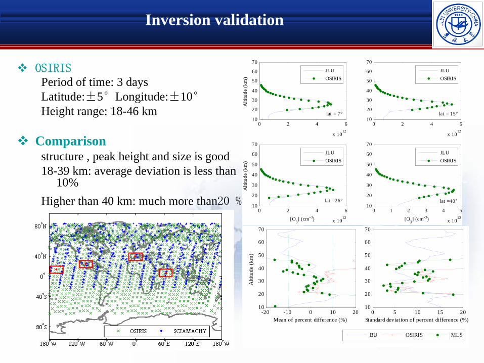
Inversion validation
OSIRISPeriod of time: 3 days Latitude:±5°Longitude:±10°Height range: 18-46 km
Comparisonstructure , peak height and size is good 18-39 km: average deviation is less than
10%Higher than 40 km: much more than20 %
0 2 4 6
x 1012
10
20
30
40
50
60
70
Alti
tude
(km
)
0 2 4 6
x 1012
10
20
30
40
50
60
70
0 2 4 6
x 1012
10
20
30
40
50
60
70
[O3] (cm-3)
Alti
tude
(km
)
0 1 2 3 4 5
x 1012
10
20
30
40
50
60
70
[O3] (cm-3)
JLUOSIRIS
JLUOSIRIS
JLUOSIRIS
JLUOSIRIS
lat =40°
lat = 15°lat = 7°
lat =26°
-20 -10 0 10 2010
20
30
40
50
60
70
Mean of percent difference (%)
Alti
tude
(km
)
0 5 10 15 2010
20
30
40
50
60
70
Standard deviation of percent difference (%)
BU OSIRIS MLS
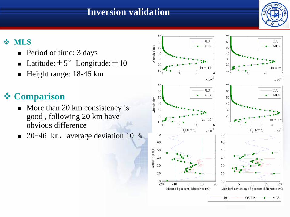
Inversion validation
MLS
Period of time: 3 days
Latitude:±5°Longitude:±10
Height range: 18-46 km
Comparison
More than 20 km consistency is good , following 20 km have obvious difference
20-46 km,average deviation 10 %
0 2 4 6
x 1012
10
20
30
40
50
60
70
Alti
tude
(km
)
0 2 4 6
x 1012
10
20
30
40
50
60
70
0 2 4 6
x 1012
10
20
30
40
50
60
70
[O3] (cm-3)
Alti
tude
(km
)
0 1 2 3 4 5
x 1012
10
20
30
40
50
60
70
[O3] (cm-3)
JLUMLS
JLUMLS
JLUMLS
JLUMLS
lat = 17° lat = 36°
lat = 2°lat = -12°
-20 -10 0 10 2010
20
30
40
50
60
70
Mean of percent difference (%)
Alti
tude
(km
)
0 5 10 15 2010
20
30
40
50
60
70
Standard deviation of percent difference (%)
BU OSIRIS MLS

Inversion validation
Comparison summary
Ozone deviation
Data Less than 10% Maximum deviation
SCIAMACHY 10-50 km 15 %
OSIRIS 18-39 km 20 %
MSL 20-46 km More than 20%
6. Conclusions
Global measurements by satellite
Limb based measurements will improve the vertical resolution of ozone concentrations
China will launch a satellite based limb ozone measurement instruments
Ground measurements will validate the satellite results. They should be integrated

Thank You!