Embed Size (px)
Citation preview


Rethinking Macroeconomics withEndogenous Market Structure


RethinkingMacroeconomics withEndogenous MarketStructure
M A R C O M A Z Z O L IUniversity of Genoa
M AT T E O M O R I N IUniversity of Torino
P I E T R O T E R N AUniversity of Torino

University Printing House, Cambridge CB2 8BS, United Kingdom
One Liberty Plaza, 20th Floor, New York, NY 10006, USA
477 Williamstown Road, Port Melbourne, VIC 3207, Australia
314–321, 3rd Floor, Plot 3, Splendor Forum, Jasola District Centre,New Delhi – 110025, India
79 Anson Road, #06–04/06, Singapore 079906
Cambridge University Press is part of the University of Cambridge.
It furthers the University’s mission by disseminating knowledge in the pursuit ofeducation, learning, and research at the highest international levels of excellence.
www.cambridge.orgInformation on this title: www.cambridge.org/9781108482608
DOI: 10.1017/9781108697019
c© Marco Mazzoli, Matteo Morini and Pietro Terna 2019
This publication is in copyright. Subject to statutory exceptionand to the provisions of relevant collective licensing agreements,no reproduction of any part may take place without the written
permission of Cambridge University Press.
First published 2019
Printed in the United Kingdom by TJ International Ltd. Padstow Cornwall
A catalogue record for this publication is available from the British Library.
Library of Congress Cataloging-in-Publication DataNames: Mazzoli, Marco, author. | Morini, Matteo, author. | Terna, Pietro, author.
Title: Rethinking macroeconomics with endogenous market structure / MarcoMazzoli, Matteo Morini, Pietro Terna.
Description: First. | New York : Cambridge university press, 2019. |Includes bibliographical references and index.
Identifiers: LCCN 2019029309 (print) | LCCN 2019029310 (ebook) |ISBN 9781108482608 (hardback) | ISBN 9781108697019 (epub)
Subjects: LCSH: Macroeconomics – Mathematical models. | Equilibrium (Economics)Classification: LCC HB172.5 .M3649 2019 (print) | LCC HB172.5 (ebook) |
DDC 339.01/51922–dc23LC record available at https://lccn.loc.gov/2019029309
LC ebook record available at https://lccn.loc.gov/2019029310
ISBN 978-1-108-48260-8 Hardback
Cambridge University Press has no responsibility for the persistence or accuracy ofURLs for external or third-party internet websites referred to in this publication
and does not guarantee that any content on such websites is, or will remain,accurate or appropriate.
Contents
List of Illustrations page ix
List of Tables xv
Notes on Contributors xviii
Introduction 1
Part One Theory 9
1 Industrial Structure and the Macroeconomy: A FewPremises for a Macromodel 111.1 Introduction 111.2 Why a New Theoretical Approach 12
1.2.1 Microfoundation 141.2.2 Market Structure 191.2.3 Expectations and Implications for the
Simulations 23
2 Industrial Structure and the Macroeconomy: TheMacroeconomic Model and Its Algebraic Framework 262.1 Introduction 262.2 The Algebraic Derivation of the Aggregate Demand 282.3 The Firms 392.4 The Incentive Compatible Wage, the Probability
of Entry and Exit and the Employment Level 482.5 A Digression on the Link Between the Labor
Market Equilibrium, the Firm’s Output and theEntry Decision 55
2.6 Interpreting the Nature of the Equilibrium in theOligopolistic Market 63
2.7 A Few Equations Summarizing the Model for theAgent-Based Simulations 67
2.8 Concluding Remarks 682.9 Technical Specifications – Entry and Output
Determination: The Existence of a Cournot-NashEquilibrium 70
v
vi Contents
Part Two Model 75
3 A Computable Market Model: The Structure of theAgent-Based Simulation 773.1 A Scheme to Start 77
3.1.1 SLAPP – Swarm-Like Agent Protocol inPython 78
3.1.2 The Structure of the Simulation Model 793.1.3 What Is a Cycle and What Are Sub-Steps? 843.1.4 Item 1: Reset Action 84
3.2 Item 2: makeProductionPlan or adaptProductionPlan 843.2.1 makeProductionPlan 843.2.2 adaptProductionPlan 85
3.3 Item 3: hireFireWithProduction 873.4 Item 4: produce 87
3.4.1 Item 4, Continuation: workTroubles 883.5 Item 5: planConsumptionInValue 883.6 Item 6: setInitialPricesHM 893.7 Item 7: actOnMarketPlace 923.8 Item 8: setMarketPrice 963.9 Item 9: evaluateProfit 973.10 Item 10: nextSellPriceJumpFHM and
nextSellPricesQHM 983.10.1 Item 10–full: nextSellPriceJumpFHM 983.10.2 Item 10–quasi: nextSellPricesQHM 99
3.11 Item 11: toEntrepreneur and toWorker 1023.11.1 Item 11: toEntrepreneur 1023.11.2 Item 11: toWorker 102
3.12 Item 12: On wages: fullEmploymentEffect andincumbentAction 1033.12.1 Item 12: fullEmploymentEffectOnWages 1033.12.2 Item 12: incumbentActionOnWages 103
4 The Results of the Simulation Agent-Based Model, inSMAC and ASHAM Modes 1064.1 Initial Results, Cases 0a (g in Figure 4.17) and 0b
(h in Figure 4.17) 1064.2 Synopsis of SMAC Experiments, from Atomistic
to Oligopolistic Markets 112
Contents vii
4.2.1 Case 1 (a in Figure 4.17): 100Entrepreneurs and 100,000 Workers 112
4.2.2 Case 2 (b in Figure 4.17): 1,000Entrepreneurs and 100,000 Workers 115
4.2.3 Case 3 (c in Figure 4.17): 10Entrepreneurs and 100,000 Workers 117
4.2.4 Case 4 (d in Figure 4.17): 20Entrepreneurs and 100,000 workers 120
4.2.5 Case 5 (e in Figure 4.17): 50Entrepreneurs and 100,000 Workers 123
4.2.6 Case 6 (f in Figure 4.17): 50 entrepreneursand 10,000 workers 125
4.2.7 Summarizing Countercyclical MarkupPresence in Cases 0a to 6 127
4.2.8 Synopsis of Cases from 0a to 6, in theSMAC Economy 127
4.3 A Qualitative Analysis of ASHAM Experiments 1364.4 Full ASHAM 138
4.4.1 Case 7: 10 Entrepreneurs and 10,000Workers, in a Stable Economy, with anIncreasing Number of Firms 138
4.4.2 Case 8: 10 Entrepreneurs and 10,000Workers, in a Stable Economy, with FirmDynamic 144
4.5 Quasi ASHAM, with the Unsold Option 1474.5.1 Case 9: 10 Entrepreneurs and 10,000
Workers, in a Nearly Stable Economy,with a Final Tight Oligopolistic Structure 147
4.6 Quasi ASHAM, with the randomUp Option 1534.6.1 Case 10: 10 Entrepreneurs and 10,000
Workers, in a Stable Economy, withInformation Shocks and a StableOligopolistic Structure 154
4.7 Quasi ASHAM, with the Profit Option 1584.7.1 Case 11: 10 Entrepreneurs and 10,000
Workers, in a Stable Economy, with aStable Oligopolistic Market 159
4.8 Synopsis of Cases from 7 to 11, in the ASHAMEconomy 163
viii Contents
4.9 Random Values On and Off, a Test in the ASHAMEnvironment 163
5 The Model Facing Empirical Data 168
Conclusions 176
Appendices 179
Appendix A The Structure of an Atomistic SimplifiedHayekian Market 181A.1 The Structure of the Model and the Warming Up
Phase 181A.2 The Atomistic Hayekian Version 182A.3 The Unstructured Version 185A.4 Two Triple Cases of Not Balancing Numbers of
Buyers and Sellers 185A.4.1 Case nBuyers � nSellers 185A.4.2 Case nBuyers � nSellers 192
A.5 Activating Idle Agents 196A.5.1 Corrupting the Simplified Hayekian
Market Model 196A.5.2 A Fundamental Unexpected By-Product 200
Appendix B The Acrostics of the Simulation Model and ItsParameters 203
Appendix C How to Run the Oligopoly Model with SLAPP 210C.1 Time Management 213
C.1.1 The Schedule.xls Formalism 214C.1.2 The observerActions and modelActions
as High Level Schedule Formalisms 217C.2 Running a Specific Experiment, with Backward
Compatibility 218C.3 Running the Code Directly Online 220
References 221
Author Index 227
Subject Index 228
Illustrations
3.1 The outline of the simulation model with its 12 items page 803.2 Case i: buyers’ price curve with 10,000 agents, εB in
[−0.09, 0.01); sellers’ price curve with 10 agents, εS in[−0.01, 0.09) 82
3.3 Case ii: buyers’ price curve with 10,000 agents, εB in[−0.11,−0.01); sellers’ price curve with 10 agents, εS
in [0.01, 0.11) 823.4 Case iii: (a) buyers’ price curve with 10,000 agents,
εB in [−0.05, 0.05); sellers’ price curve with 10 agents,εS in [−0.05, 0.05) 83
3.5 Case iii: (b) buyers’ price curve with 10,000 agents,εB in [−0.10, 0.10); sellers’ price curve with 10 agents,εS in [−0.10, 0.10) 83
4.1 Case 0a from the 2017 paper, macro-variable serieswith new entrant firms 108
4.2 Case 0a from the 2017 paper, agent series with newentrant firms 108
4.3 Case 0b from the 2017 paper, macro-variable serieswithout new entrant firms 109
4.4 Case 0b from the 2017 paper, agent series withoutnew entrant firms 109
4.5 Case 1, 100 entrepreneurs and 100,000 workers,macro-variable series 113
4.6 Case 1, 100 entrepreneurs and 100,000 workers,agent series 114
4.7 Case 2, 1,000 entrepreneurs and 100,000 workers,macro-variable series 116
4.8 Case 2, 1,000 entrepreneurs and 100,000 workers,agent series 116
4.9 Case 3, 10 entrepreneurs and 100,000 workers,macro-variable series 118
ix
x List of Illustrations
4.10 Case 3, 10 entrepreneurs and 100,000 workers, agentseries 118
4.11 Case 4, 20 entrepreneurs and 100,000 workers,macro-variable series 120
4.12 Case 4, 20 entrepreneurs and 100,000 workers, agentseries 121
4.13 Case 5, 20 entrepreneurs and 100,000 workers,macro-variable series 124
4.14 Case 5, 20 entrepreneurs and 100,000 workers, agentseries 124
4.15 Case 6, 50 entrepreneurs and 10,000 workers,macro-variable series 126
4.16 Case 6, 50 entrepreneurs and 10,000 workers, agentseries 126
4.17 A scatter plot from Table 4.25 (SMAC cases) 1324.18 Case 7, 10 entrepreneurs and 10,000 workers, macro-
variable series. The plannedP line is superimposed tothe totalProd line 140
4.19 Case 7, 10 entrepreneurs and 10,000 workers, agentseries 141
4.20 Case 7b, 10 entrepreneurs and 10,000 workers,macro-variable series. The wage line is superimposedto the hPSd line. The plannedP line is superimposedto the totalProd line 143
4.21 Case 8, 10 entrepreneurs and 10,000 workers, macro-variable series. The plannedP line is superimposed tothe totalProd line 145
4.22 Case 8, 10 entrepreneurs and 10,000 workers, agentseries 146
4.23 Case 8b, 10 entrepreneurs and 10,000 workers,macro-variable series. The wage line is superimposedto the hPSd line. The plannedP line is superimposedto the totalProd line 147
4.24 Case 9, 10 entrepreneurs and 10,000 workers, macro-variable series. The plannedP line is superimposedto the totalProd line, but the value at pos. 21 on thex-axis 150
4.25 Case 9, 10 entrepreneurs and 10,000 workers, agentseries 151
List of Illustrations xi
4.26 Case 9b, 10 entrepreneurs and 10,000 workers,macro-variable series. The plannedP line issuperimposed to the totalProd line, but the value atpos. 28 on the x-axis 153
4.27 Case 9b, 10 entrepreneurs and 10,000 workers, agentseries 154
4.28 Case 10, 10 entrepreneurs and 10,000 workers,macro-variable series. The plannedP line issuperimposed to the totalProd line 156
4.29 Case 10, 10 entrepreneurs and 10,000 workers, agentseries 156
4.30 Case 11, 10 entrepreneurs and 10,000 workers,macro-variable series. The plannedP line issuperimposed to the totalProd line, but the value atpos. 19 on the x-axis 161
4.31 Case 11, 10 entrepreneurs and 10,000 workers, agentseries 161
4.32 Case 8modPars, 10 entrepreneurs and 10,000workers, macro-variable series. The plannedP line issuperimposed to the totalProd line 166
4.33 Case 8modPars, 10 entrepreneurs and 10,000workers, agent series 166
5.1 Births and deaths of enterprises (x 1,000) 1695.2 Ratio births/deaths enterprises 1695.3 Birth/deaths enterprise ratio versus GDP rate of
change 1705.4 The dynamic of the markup 1715.5 GDP dynamic–markup–births/deaths ratio of the
enterprises 171A.1 An example of initially not overlapping buyers’ price
curve (black) and sellers’ price curve (gray) 183A.2 Simplified Hayekian case: (i) an example of final
buyers’ price and sellers’ price curves, (ii) the historyof mean prices tick-by-tick, (iii) their coefficients ofvariation within each tick (cycle) 184
A.3 Simplified Hayekian case: (i) the distribution of meanprices of each cycle (i.e., tick-by-tick) and (ii) that oftheir standard deviations within each tick (cycle) 184
xii List of Illustrations
A.4 Unstructured case: (i) an example of final buyers’price and sellers’ price curves, (ii) the history of meanprices tick-by-tick, (iii) their coefficients of variationwithin each tick (cycle) 186
A.5 Unstructured case: (i) the distribution of mean pricesof each cycle (i.e., tick-by-tick) and (ii) that of theirstandard deviations within each tick (cycle) 186
A.6 An example of initially not overlapping buyers’ priceand sellers’ price curves, case nBuyers � nSellers 187
A.7 Simplified Hayekian case, with nBuyers � nSellers:(i) an example of final buyers’ price and sellers’ pricecurves, (ii) the history of mean prices tick-by-tick, (iii)their coefficients of variation within each tick (cycle) 188
A.8 Simplified Hayekian case, with nBuyers � nSellers:(i) the distribution of mean prices of each cycle (i.e.,tick-by-tick) and (ii) that of their standard deviationswithin each tick (cycle) 188
A.9 Simplified Hayekian case, with nBuyers � nSellersbut with equivalent effects: (i) an example of finalbuyers’ price and sellers’ price curves, (ii) the historyof mean prices tick-by-tick, (iii) their coefficients ofvariation within each tick (cycle) 190
A.10 Simplified Hayekian case, with nBuyers � nSellersbut with equivalent effects: (i) the distribution ofmean prices of each cycle (i.e., tick-by-tick) and (ii)that of their standard deviations within each tick(cycle) 190
A.11 Simplified Hayekian case, with nBuyers � nSellersbut squeezing the effects: (i) an example of finalbuyers’ price and sellers’ price curves, (ii) the historyof mean prices tick-by-tick, (iii) their coefficients ofvariation within each tick (cycle) 191
A.12 Simplified Hayekian case, with nBuyers � nSellersbut squeezing the effects: (i) the distribution of meanprices of each cycle (i.e., tick-by-tick) and (ii) that oftheir standard deviations within each tick (cycle) 191
A.13 An example of initially not overlapping buyers’ priceand sellers’ price curves, case nBuyers � nSellers 192

List of Illustrations xiii
A.14 Simplified Hayekian case, with nBuyers � nSellers:(i) an example of final buyers’ price and sellers’ pricecurves, (ii) the history of mean prices tick-by-tick, (iii)their coefficients of variation within each tick (cycle) 193
A.15 Simplified Hayekian case, with nBuyers � nSellers:(i) the distribution of mean prices of each cycle (i.e.,tick-by-tick) and (ii) that of their standard deviationswithin each tick (cycle) 194
A.16 Simplified Hayekian case, with nBuyers � nSellerswith equivalent effects: (i) an example of final demandand offer curves, (ii) the history of mean pricestick-by-tick, (iii) their coefficients of variation withineach tick (cycle) 195
A.17 Simplified Hayekian case, with nBuyers � nSellersbut with equivalent effects: (i) the distribution ofmean prices of each cycle (i.e., tick-by-tick) and(ii) that of their standard deviations within each tick(cycle) 195
A.18 Simplified Hayekian case, with nBuyers � nSellersbut squeezing the effects: (i) an example of finalbuyers’ price and sellers’ price curves, (ii) the historyof mean prices tick-by-tick, (iii) their coefficients ofvariation within each tick (cycle) 197
A.19 Simplified Hayekian case, with nBuyers � nSellersbut squeezing the effects: (i) the distribution of meanprices of each cycle (i.e., tick-by-tick) and (ii) that oftheir standard deviations within each tick (cycle) 197
A.20 Corrupting the simplified Hayekian case: (i) anexample of final buyers’ price and sellers’ pricecurves, (ii) the history of mean prices tick-by-tick, (iii)their coefficients of variation within each tick (cycle) 199
A.21 Corrupting the simplified Hayekian case: (i) thedistribution of mean prices of each cycle (i.e.,tick-by-tick) and (ii) that of their standard deviationswithin each tick (cycle) 199
A.22 Extending the simplified Hayekian case: after 10,000actions we see here a flash image of the buyersordered following their reservation prices, with the
xiv List of Illustrations
number of recent consecutive unsuccessful buyingattempts 200
A.23 Extending the simplified Hayekian case: (i) anexample of final buyers’ price and sellers’ pricecurves, (ii) the history of mean prices tick-by-tick,(iii) their coefficients of variation within each tick(cycle) 201
A.24 Extending the simplified Hayekian case: (i) thedistribution of mean prices of each cycle (i.e.,tick-by-tick) and (ii) that of their standard deviationswithin each tick (cycle) 202
A.25 Extending the simplified Hayekian case: after 20,000actions, each buyer (here the buyers are orderedfollowing their reservation prices) has been successfulin concluding a deal only in about 10,000 cases 202
C.1 The representation of the schedule 213

Tables
4.1 Legends page 1074.2 Case 0a from the 2017 paper, correlations with new
entrant firms 1104.3 Case 0a from the 2017 paper, partial correlations
(excluding plannedProduction) with new entrantfirms 111
4.4 Case 0a from the 2017 paper, partial correlations(excluding totalProduction) with new entrant firms 111
4.5 Case 0b from the 2017 paper, correlations withoutnew entrant firms 112
4.6 Case 1, 100 entrepreneurs and 100,000 workers,correlations 114
4.7 Case 1, partial correlations (excludingplannedProduction) 115
4.8 Case 1, partial correlations (excludingtotalProduction) 115
4.9 Case 2, 1,000 entrepreneurs and 100,000 workers,correlations 117
4.10 Case 2, partial correlations (excludingplannedProduction) 117
4.11 Case 2, partial correlations (excludingtotalProduction) 119
4.12 Case 3, 10 entrepreneurs and 100,000 workers,correlations 119
4.13 Case 4, 20 entrepreneurs and 100,000 workers,correlations 119
4.14 Case 4, partial correlations (excludingplannedProduction) 122
4.15 Case 4, partial correlations (excludingtotalProduction) 122
xv
xvi List of Tables
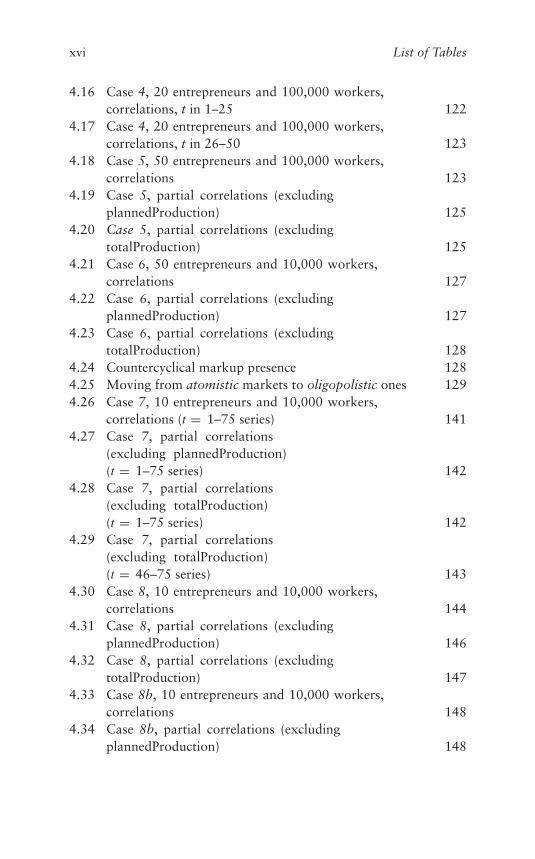
4.16 Case 4, 20 entrepreneurs and 100,000 workers,correlations, t in 1–25 122
4.17 Case 4, 20 entrepreneurs and 100,000 workers,correlations, t in 26–50 123
4.18 Case 5, 50 entrepreneurs and 100,000 workers,correlations 123
4.19 Case 5, partial correlations (excludingplannedProduction) 125
4.20 Case 5, partial correlations (excludingtotalProduction) 125
4.21 Case 6, 50 entrepreneurs and 10,000 workers,correlations 127
4.22 Case 6, partial correlations (excludingplannedProduction) 127
4.23 Case 6, partial correlations (excludingtotalProduction) 128
4.24 Countercyclical markup presence 1284.25 Moving from atomistic markets to oligopolistic ones 1294.26 Case 7, 10 entrepreneurs and 10,000 workers,
correlations (t = 1–75 series) 1414.27 Case 7, partial correlations
(excluding plannedProduction)(t = 1–75 series) 142
4.28 Case 7, partial correlations(excluding totalProduction)(t = 1–75 series) 142
4.29 Case 7, partial correlations(excluding totalProduction)(t = 46–75 series) 143
4.30 Case 8, 10 entrepreneurs and 10,000 workers,correlations 144
4.31 Case 8, partial correlations (excludingplannedProduction) 146
4.32 Case 8, partial correlations (excludingtotalProduction) 147
4.33 Case 8b, 10 entrepreneurs and 10,000 workers,correlations 148
4.34 Case 8b, partial correlations (excludingplannedProduction) 148
List of Tables xvii
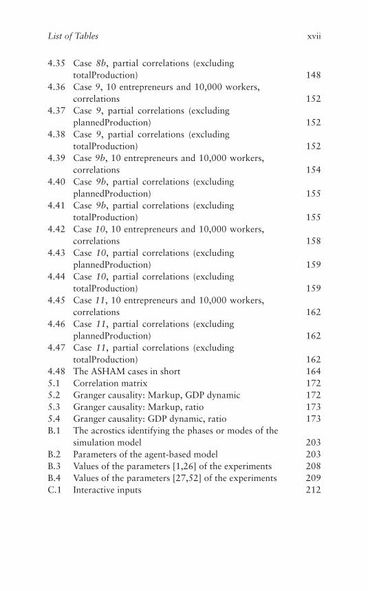
4.35 Case 8b, partial correlations (excludingtotalProduction) 148
4.36 Case 9, 10 entrepreneurs and 10,000 workers,correlations 152
4.37 Case 9, partial correlations (excludingplannedProduction) 152
4.38 Case 9, partial correlations (excludingtotalProduction) 152
4.39 Case 9b, 10 entrepreneurs and 10,000 workers,correlations 154
4.40 Case 9b, partial correlations (excludingplannedProduction) 155
4.41 Case 9b, partial correlations (excludingtotalProduction) 155
4.42 Case 10, 10 entrepreneurs and 10,000 workers,correlations 158
4.43 Case 10, partial correlations (excludingplannedProduction) 159
4.44 Case 10, partial correlations (excludingtotalProduction) 159
4.45 Case 11, 10 entrepreneurs and 10,000 workers,correlations 162
4.46 Case 11, partial correlations (excludingplannedProduction) 162
4.47 Case 11, partial correlations (excludingtotalProduction) 162
4.48 The ASHAM cases in short 1645.1 Correlation matrix 1725.2 Granger causality: Markup, GDP dynamic 1725.3 Granger causality: Markup, ratio 1735.4 Granger causality: GDP dynamic, ratio 173B.1 The acrostics identifying the phases or modes of the
simulation model 203B.2 Parameters of the agent-based model 203B.3 Values of the parameters [1,26] of the experiments 208B.4 Values of the parameters [27,52] of the experiments 209C.1 Interactive inputs 212

Notes on Contributors
Marco Mazzoli is associate professor of Economic Policy at the Uni-versity of Genoa (Italy). He holds a PhD in Economics from the Uni-versity of Warwick. He has published various papers in internationaljournals and, with Cambridge University Press, he published in 1998the research monograph Credit, Investments and the Macroeconomy.His research fields include macroeconomics, monetary economics andfinancial markets.
Matteo Morini got his PhD at the Ecole Normale Supérieure deLyon, France; he works on complex networks, and develops agent-based and econometric models at the University of Torino. He isalso employed at the Institut für Wirtschafts- und Verwaltungsinfor-matik at the Universität Koblenz-Landau, teaches courses on complexsystems in the Carlo Alberto postgraduate programme and sits inthe board of directors (as vice-president) of the Swarm DevelopmentGroup. He co-authored and co-edited two books on complexity andABMs. For more of his work, see http://perso.ens-lyon.fr/matteo.morini.
Pietro Terna is a retired professor of the University of Torino (Italy),where he was a full professor of economics. His research work is inthe fields of (i) artificial neural networks for economic applicationsand (ii) social simulation with agent-based models (where he has beenpioneering the use of Swarm, www.swarm.org). He has prepared anew agent-based simulation tool in Python (Swarm-Like Agent Pro-tocol in Python), SLAPP (https://terna.github.io/SLAPP/),deriving it from the Swarm project. He is currently teaching a courseon econophysics for the master degree in physics for complex systemsat the University of Torino. His publications and projects can be foundat https://terna.to.it.
Simone Lombardini is a PhD student at the University of Genoa,Italy, where he got his master’s degree in economics and financial
xviii

Notes on Contributors xix
institutions, and is currently visiting the University of Oslo, Norway.Recently, he published a book on Inequality and Poverty in ModernCapitalism, in Italian. His research interests include business cycles,finance, inflation and income distribution.

Introduction
Do entry, exit and changes in market structure affect the macroe-conomy? Is there a link between the strategic interactions amongoligopolistic firms and the macroeconomic equilibrium? The questionis certainly not trivial in modern economies, where large oligopolis-tic firms play a relevant role and so many meetings among statesmenhave the explicit scope of promoting contracts for some large andimportant firms of their countries. However, surprisingly enough, themost popular theoretical models in the modern macroeconomic lit-erature hardly see any explicit formalization for the macroeconomiceffects of changes in market structure, entry, exit and strategic inter-actions among oligopolists, if not as mere mechanic and secondaryeffects of the usual technology shocks, commonly invoked as thecause of business cycle. Do we really think that the sophisticatedstrategies of large firms’ decision makers do not carry any macroeco-nomic consequences? The market structure and strategic interactionsamong oligopolists are not necessarily associated with scale economiesor technology shocks. In order to better focus on this point, thetheoretical model of this book describes, like some of the most impor-tant original contributions in the conventional DSGE literature, aneconomy where the labor is the only production input.
This book deals with all these issues by introducing a new macroe-conomic approach: Part 1 provides its theoretical background andmodeling framework, and Part 2 its implications by running somesimulations and comparing the results with the US macroeconomicdata.
A feature of our model is endogenous market structure, explic-itly built to account for its feedback with the aggregate variables: inparticular, changes in market structure are a potential cause of macroe-conomic fluctuations and business cycle, and this is formalized byplugging into a macromodel a theoretical mechanism of entry and exit
1
2 Introduction
that also allows to keep track of aggregate output, market size, socialmobility and income distribution. What we mean to create is a generalframework that may be adapted (by specifying less general and moredetailed features) to model specific assumptions and phenomena. Inthis sense, the perspective of our book is different from the contribu-tions focused on the statistical properties of oligopolistic markets oron the statistical distribution of firm size.
Our framework also provides a theory to interpret markups overthe business cycle according to the feasibility of entry: in particular,Chapter 4 also includes a simulation where countercyclical markupemerges as a consequence of large entry and disappears in the case ofblocked entry.
Lee and Mukoyama (2018) introduce a general equilibrium modelto account for entry and exit over the business cycle, assuming thatthe entry costs are cyclical. While the only point in common with ourwork is that the entry and exit rates are determined by an endogenousmechanism, we focus instead on the fact that in an oligopolistic econ-omy entry and exit cannot be explained without explicitly consideringand modeling the strategic interactions among the oligopolistic firms.Therefore, without loss of generality, we do not need to assume thatentry costs are cyclical, we do not need to make any specific assump-tion on the statistical or empirical configuration of firms’ size and wemainly model the logical links between macroeconomic facts and deci-sions of the entrepreneurs and potential entrants. In this regard, weintroduce a theory of information spreading and individuals decisionmaking consistent with a fairly general notion of rationality and, morespecifically, even with the notion of rational expectations.
We believe that introducing this perspective as the theoretical back-ground of agent-based macroeconomic simulations constitutes aninteresting point in itself. Apart from introducing a new microfoundedtheoretical model that explains the business cycle as an effect ofentry/exit, interpreted as strategic decisions of the firms and intro-ducing, in this regard, a general notion of rationality also broadlyconsistent with the assumption of rational expectations, we pro-duce simulations and appropriate predictions for the macroeconomicfluctuations based on the agent-based methodology.
To develop the last paragraph, let us describe the Agent-Based Mod-els (ABMs) field in a few steps. We follow – with some modifications –the specifications of two of the pioneers of the field, Robert Axtell and
Introduction 3
Joshua M. Epstein, particularly in the description of the ABMs thatthey introduce in Axtell and Epstein (2006).
i) The starting point is a population of agents, representing individ-uals or, more generally, entities as the component of a genericsystem that we construct using small parts of computer codeoperating in dedicated software environments.
ii) The goal is to search for regularities at the macro level generatedby the behavior of the agents (micro level, if individuals; mesolevel, if more complex entities).
iii) An ABM does not introduce equations governing the effects ofthe agents’ behavior at the macro level, but it allows us to observethe emergence of those effects (i.e., summing up the outcomes ofthe actions and interactions of the agents).
iv) Agents, on their side, can use equations to assume their decisions;equations can be very complicated (e.g., produced via artificialneural networks or other artificial intelligence algorithms). Agentscan also learn from their errors, modifying the internal equationsor artificial neural networks. In this book, their action is based onthe sequence described in Chapter 3, and particularly in Figure3.1.
v) Heterogeneity is usual in ABMs, and as a consequence, the agentshave different internal structures.
vi) With ABMs we can manage boundedly rational behavior, non-equilibrium dynamics, and spatial processes.
vii) Regularly, the coding techniques are based on object-oriented pro-gramming and build the agents using instances of classes, where agood class synonym is set.
In our model, the agent-based technique allows us to emphasizethe role of strategic interaction among oligopolistic firms, as theconsequence of subjective decision making, formalizing in the mostappropriate way the implication and results of these decisions. Weproduce all the actions and reactions designed by the model equationsvia the behavior of heterogeneous agents actually acting in the sim-ulated time. We remark that between (a) the formal presentation ofthe model in the equation based way, strictly necessary to be consis-tent with the literature upon which our work is grounded, and (b)the agent-based implementation, the consistency is deeply satisfied,but with a few inevitable distinctions. The same kind of differences
4 Introduction
that we run up against when we compare (a) the formalization of aphenomenon and (b) the related observation of the reality (here: anartificial one, simulated).
We hope that the framework introduced in this book may be a use-ful tool for further research and extensions, where the endogeneity ofmarket structure in a macromodel and its potential implications is adistinguished feature.
Rationale, Scope and Contribution of the Bookto the Existing Literature
The last decade has seen a lively debate in macroeconomics, with anincreasing criticism on the model that seemed to be dominant in lit-erature since the end of the 1990s, the Dynamic Stochastic GeneralEquilibrium (DSGE, hereafter), and, consequently, the birth of somenew theoretical approaches and methodologies.
In spite of the heroic defense of the DSGE approach introduced byChristiano et al. (2018), the serious drawbacks of that class of modelsis clearly described by Romer (2016), who explicitly talks about lackof scientific background. However, we believe that the general notionof general equilibrium, in dynamics terms, is not ill-based, and for thisreason, our theoretical model has still the nature of a general equilib-rium model, although its premises are completely different from thoseof the conventional DSGE literature.
On our side, we have the double feature of ABMs: to be close to anarrative of the reality, thanks to their flexibility, but most of all, tobe close to a mathematical model, thanks to a rigorous representationvia a computer code.
With Lengnick (2013) we can argue that
[. . . ] agent-based modeling is an adequate response to the recently expressedcriticism of macroeconomic methodology because it allows for aggregatebehavior that is more than simply a replication of microeconomic opti-mization decisions in equilibrium. At the same time it allows for absolutelyconsistent microfoundations, including the structure and properties of mar-kets. Most importantly, it does not depend on equilibrium assumptions orfictitious auctioneers and does therefore not rule out coordination failures,instability and crisis by definition. A situation that is very close to a generalequilibrium can instead be shown to result endogenously from non-rationalmicro interaction.
Introduction 5
Important contributions in this direction come from Di Guilmi et al.(2017). A different criticism on the DSGE paradigm is expressed inWiesner et al. (2019), where the questionable role of DSGE modelsis inserted in an analysis of the stability of democracies in a complexsystems perspective.
Consistent with the last context is the famous Trichet (2010) obser-vation, when he was close to leave the role of President of theEuropean Central Bank:
As a policy-maker during the crisis, I found the available models of limitedhelp. In fact, I would go further: in the face of the crisis, we felt aban-doned by conventional tools. [. . . ] We do not need to throw out our DSGEand asset-pricing models: rather we need to develop complementary toolsto improve the robustness of our overall framework. [. . . ] First, we haveto think about how to characterise the homo economicus at the heart ofany model. The atomistic, optimising agents underlying existing models donot capture behaviour during a crisis period. We need to deal better withheterogeneity across agents and the interaction among those heterogeneousagents. We need to entertain alternative motivations for economic choices.Behavioural economics draws on psychology to explain decisions made incrisis circumstances. Agent-based modelling dispenses with the optimisationassumption and allows for more complex interactions between agents. Suchapproaches are worthy of our attention.
Ghorbani et al. (2014), whose article has the descriptive titleEnhancing ABM into an Inevitable Tool for Policy Analysis, workin the same direction, proposing to use a coordinated rich set ofinstruments for policies.
The novelty of our book is also that of introducing a completely newtheoretical framework whose purpose is modeling a stylized fact thathas been partly neglected in macroeconomic research: the reciprocalinteractions between industrial structure and the macroeconomy in aneconomy with large oligopolistic firms. Entry and exit in an oligopolis-tic economy are phenomena with a large enough magnitude to affectthe macroeconomic equilibrium, and most economists would agreewith the fact that the birth and death of firms is an empirical phe-nomenon associated with the business cycle or, perhaps, one of themain empirical features of the business cycle.
Our theoretical framework is also useful to analyze the behav-ior of the firms’ markups over the cycle in a (realistic) world whereindividuals are heterogeneous in their budget constraints: they can be
6 Introduction
workers, or new entrant entrepreneurs, or incumbent entrepreneurs orunemployed and may change their status when they take a drastic deci-sion (i.e., using the language and metaphors of economists, when theyare affected by informational shocks). The aggregate demand is micro-founded and explicitly modeled as the sum of the individual demands.Another realistic feature of our theoretical model is that oligopolisticfirms and heterogeneous agents have, in general, diverging incentives(Aoki and Yoshikawa, 2007). The algebraic structure of our modelmay also be used as an analytical framework for the links amongentry/exit, social mobility and the macroeconomy.
In Chapter 5, we report actual data related to our main research pat-tern, i.e., the emergence of the countercyclical markup. We aware ofthe open issue of ABMs validation and the methodological contribu-tion of Fagiolo et al. (2007), but we remark that out main purpose hereis to build a reasoning machine. Broadly, these might be summarizedas a pattern oriented modeling approach, and we can do many-leveled,qualitative logical validations. For an interesting open discussion onvalidation, refer to Malleson (2018).
We could do a many leveled, qualitative validation. We can checkthat the outcome distributions are the right shape (or other knownfacts about people) to simultaneously constrain the simulation inmany aspects, dimensions and scales at once.
This work is a research book, mainly addressed to postgradu-ate students, PhD students, professional economists and researchers.If you are not interested in the full details, please simply read theIntroduction and Chapters 1, 2 and 4. If possible, refer to Appendix A.
An overview
In Chapter 1, we briefly discuss the rationale and the premises forthe theoretical model of the book and how our theoretical modelrelates to the existing and related literature. The model describes aneconomy with an oligopolistic industrial sector, and our purpose is toanalyze the interactions between the market structure and the macroe-conomy – in particular, how the equilibrium among the oligopolisticfirms impacts the macroeconomy and how the macroeconomy in turnimpacts the equilibrium among the oligopolistic firms.
In Chapter 2, we have the structure of the model, built plugging theentry/exit decisions into a macroeconomic system, by using a notion ofstatistical distribution of expectations that is consistent with the idea
Introduction 7
of rational expectations (at least in its original formulation) to modelthe entry decision of potential entrants. The theoretical framework isalso useful to analyze, on a theoretical ground, the behavior of thefirms’ markups over the cycle and is employed for the agent-basedsimulations. In particular, we model a macroeconomic system witholigopoly, entry/exit and heterogeneous individuals.
In Chapter 3, starting from the equation based construction intro-duced in Chapter 2, we build a macroeconomic simulation model of aneconomic using the agent-based technique; the model is microfounded,and so our explanation starts from the behavior of the agents and ofthe market frameworks where they behave. The structure of the sim-ulation model is well represented via the sequence of the 12 items ofFigure 3.1.
In Chapter 4, we analyze the simulation results, considering boththe dynamic of the time series of the main economic variables of themodel and their correlation structure. The attention is mainly relatedto the emergence of the countercyclical markup phenomenon and tothe dynamics of the market structures, ranging from tight oligopolisticconstructions to the development of large atomistic markets.
In Chapter 5 we propose some actual data related to the GDPcycle and to the income components, to search for the presence ofthe countercyclical markup.
Appendix A is dedicated to a digression on decentralized marketbased on agents, and it is useful to understand the background ofChapter 4.
Appendix B introduces the collection of the parameters (names andvalues) used in the book.
Appendix C explains how to run the code, with some documentedexception for the different cases of Chapter 4.
Online Resources
The code has a reference handbook, Oligopoly: the Making of the Sim-ulation Model,1 that describes the details of the program, complyingwith the AEA Data Availability Policy.2
1 Online at https://terna.github.io/oligopoly/Oligopoly.pdf .2 https://www.aeaweb.org/journals/policies/data-availability-policy .

8 Introduction
Online we have also the whole oligopoly code,3 and the SLAPPshell,4 employed to run the model in the way pointed sub vii) above.
Acknowledgments
First of all, a huge thanks to Eleonora Priori,5 for her thorough andpassionate comments and suggestions. We are also deeply grateful toa special reader, Dr. Simone Landini,6 for his precious review of themanuscript. The very valuable comments from the Cambridge Univer-sity Press anonymous referees have been extremely useful to improveour work and are gratefully acknowledged.
Thanks for their suggestions and encouragements to Giorgio Rampaand Federico Boffa.
Thanks to the Italian scholars in agent-based simulation, for cre-ating a favorable environment for this kind of research. We remindthe groups quoted in Dosi and Roventini (2017): the Scuola Superi-ore Sant’Anna (Pisa); the so called CATS family, developed betweenAncona and Milano; the EURACE model, born in the University ofGenova. A group has also been alive in Torino.
3 https://github.com/terna/oligopoly .4 At https://terna.github.io/SLAPP/ or at https://github.com/terna/SLAPP .
5 Currently (2018) a student of the Vilfredo Pareto doctoral school in Economicsof the University of Torino
6 I.R.E.S Piemonte, Torino, Italy
PART ONE
Theory

1 Industrial Structure and theMacroeconomy: A Few Premisesfor a Macromodel
MARCO MAZZOLI
1.1 Introduction
This chapter briefly discusses the rationale and the premises for thetheoretical model of this book and how our theoretical model relatesto the existing and related literature. As discussed in the next chapter,our model describes an economy with an oligopolistic industrial sec-tor, and our purpose is to analyze the interactions between the marketstructure and the macroeconomy. In particular, how does the equi-librium among the oligopolistic firms impact the macroeconomy, andhow does the macroeconomy impact back on the equilibrium amongthe oligopolistic firms?
The birth and death of firms is not just an empirical fact associatedwith the business cycle: it is the heart of the business cycle and themacroeconomic effects of the equilibrium and strategic interactionsemerging among the firms operating in an economy with oligopolisticmarkets are likely to be non-negligible.
More generally, we state that diverging incentives betweenoligopolistic firms and heterogeneous agents may play a relevantmacroeconomic role. Entry and exit respectively generate or eliminatenew entrepreneurs with firms and workers. In this sense, a macro-model that explicitly models the causes or incentives for entry/exit,markups, employment/unemployment may shed a new light for under-standing the possible causal links among market structure, socialmobility and the macroeconomic trends if one removes the assump-tion (rather conventional in the DSGE literature) that individuals areat the same time entrepreneurs and workers and therefore each ofthem, rather hilariously, negotiates with himself his wage. A modelwith these features could also provide a general framework to analyzethe behavior of markups over the business cycle.
Each individual’s expectation constitutes a point along the curveof frequency of the distribution of expectations. The average of such
11
12 Marco Mazzoli
frequency distributions corresponds to the market’s rational expecta-tion. In this sense, the model is consistent with the rational expectationidea that the individuals’ expectations are “on average” correct inpredicting the relevant market variables. The agents, in their ratio-nality, are aware of the existence of a distribution of expectations(i.e., a distribution of individually heterogeneous expectations butwith a “correct average”) and, for this reason, make the adjustmentattempts described in Chapter 3. In this sense, the agent-based sim-ulations constitute a link between theory and reality that actuallyexplains how they attempt to know the “correct” market average ofexpectations (not known a priori by them) by making sequences ofattempts.
The theoretical premises of this book, therefore, are rather differentfrom those of the “behavioral new Keynesian model,” introduced inthe seminal works by De Grauwe (2011), De Grauwe and Kaltwasser(2012), Branch and McGough (2010), and Branch and McGough(2016), who incorporated the agent-based computational techniquesinto conventional DSGE models.
The next section and all its subsections briefly discuss why thetheoretical premises of our model could not be developed within a con-ventional DSGE framework and in what regards our model is differentfrom that class of models and from other existing macroeconomicapproaches.
The last section of this chapter contains some final remarks andintroduces the basic assumptions contained in the model of the nextchapter.
1.2 Why a New Theoretical Approach
Discussing how the literature on agent-based computational eco-nomics relates to the DSGE models and analyzing all the variousforms of criticism toward the DSGE models is well beyond the pur-pose of this book, and several excellent surveys exist in this regard,like, for instance, Dilaver et al. (2018) or, for what concerns the policyimplications, Fagiolo and Roventini (2017). In this chapter, we focusinstead on a specific causal link and modeling feature that has beenrelatively neglected by the conventional macroeconomic and DSGEliterature: the (reciprocal) link between industrial structure and themacroeconomy.
Premises for a Macromodel 13
The class of models sometimes denominated as “macroeconomicsfrom the bottom up” (Delli Gatti et al., 2005, 2010, 2011; Gaffeoet al., 2008) follows the evolutionary economics approach, includesagents’ heterogeneity and bounded rationality and often refers tocomplexity theory. More precisely, these models usually focus on themacroeconomic outcomes emerging from firm heterogeneity in thetransmission and amplification of shocks. Instead of focusing theanalysis on the notion of equilibrium, it is the concept of “emer-gence” of a macroeconomic state that is the leading methodologicalconcept.
Lee and Mukoyama (2018) provide a very remarkable paper, wherestochastic productivity shocks affect the dynamics of plant invest-ments and, in this way, the business cycle. Like in the conventionalbusiness cycle literature, the productivity shocks are the very causeof business cycle and, as a consequence, of the rate of entry, whichare then ultimately still related to productivity shocks. Clementi andPalazzo (2016) extend Lee and Mukoyama’s model (as it appears ina previous version) by including capital stocks, which play the impor-tant empirical role of generating a propagation mechanism. Previouscontributions, like Veracierto (2002, 2008), assumed exogenous entryand exit, while Comin and Gertler (2006), in a model with endogenousinnovation and technology adoption, endogenously explain entry,while exit is still exogenous. In this sense, Lee and Mukoyama, byassociating entry and exit to productivity shocks, certainly provide asignificant contribution, although they do not explicitly model capitalstock and land (Lee and Mukoyama, 2018, p. 10). Differently fromthem, in our model, entry and exit are associated with the (heteroge-neous) profits level and not with the mere productivity shock, whileentry and exit interact with the macroeconomic equilibrium, and, asa consequence, the macroeconomic price level is not only determinedby wages.
Dosi et al. (2006, 2008, 2010) introduce a new class of mod-els, sometimes denominated “Keynes meets Schumpeter.” Instead offocusing on complexity, they put their emphasis on the heterogene-ity of agent types. Their critique of the real business cycle and “NewKeynesian DSGE” is based on the fact that the explanation of themacroeconomic fluctuations in these two approaches mainly relyon exogenous and stochastic technology shocks and undervalue therelevance of endogenous technology innovation. Having introduced
14 Marco Mazzoli
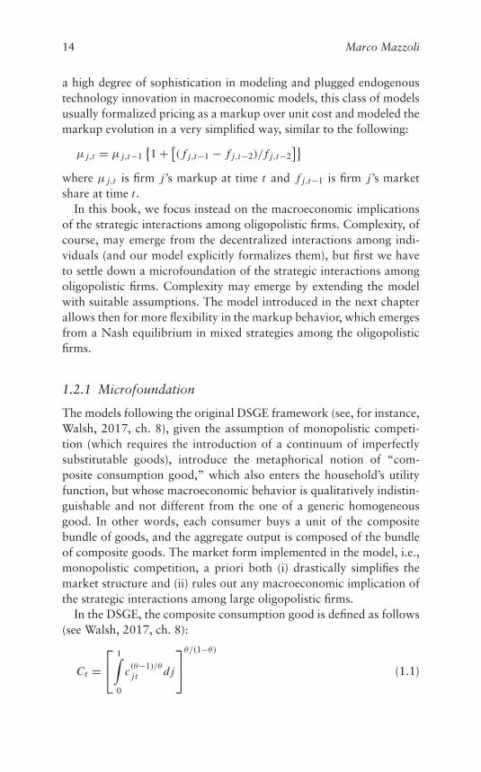
a high degree of sophistication in modeling and plugged endogenoustechnology innovation in macroeconomic models, this class of modelsusually formalized pricing as a markup over unit cost and modeled themarkup evolution in a very simplified way, similar to the following:
μ j,t = μ j,t−1{1 + [
( f j,t−1 − f j,t−2)/ f j,t−2]}
where μ j,t is firm j ’s markup at time t and f j,t−1 is firm j ’s marketshare at time t .
In this book, we focus instead on the macroeconomic implicationsof the strategic interactions among oligopolistic firms. Complexity, ofcourse, may emerge from the decentralized interactions among indi-viduals (and our model explicitly formalizes them), but first we haveto settle down a microfoundation of the strategic interactions amongoligopolistic firms. Complexity may emerge by extending the modelwith suitable assumptions. The model introduced in the next chapterallows then for more flexibility in the markup behavior, which emergesfrom a Nash equilibrium in mixed strategies among the oligopolisticfirms.
1.2.1 Microfoundation
The models following the original DSGE framework (see, for instance,Walsh, 2017, ch. 8), given the assumption of monopolistic competi-tion (which requires the introduction of a continuum of imperfectlysubstitutable goods), introduce the metaphorical notion of “com-posite consumption good,” which also enters the household’s utilityfunction, but whose macroeconomic behavior is qualitatively indistin-guishable and not different from the one of a generic homogeneousgood. In other words, each consumer buys a unit of the compositebundle of goods, and the aggregate output is composed of the bundleof composite goods. The market form implemented in the model, i.e.,monopolistic competition, a priori both (i) drastically simplifies themarket structure and (ii) rules out any macroeconomic implication ofthe strategic interactions among large oligopolistic firms.
In the DSGE, the composite consumption good is defined as follows(see Walsh, 2017, ch. 8):
Ct =⎡⎣ 1∫
0
c(θ−1)/θj t d j
⎤⎦θ/(1−θ)
(1.1)
Premises for a Macromodel 15
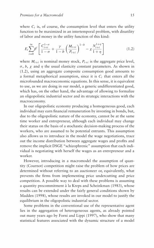
where Ct is, of course, the consumption level that enters the utilityfunction to be maximized in an intertemporal problem, with disutilityof labor and money in the utility function of this kind:
Et
∞∑i=0
β i
[C1−σ
t+i
1 − σ+ γ
1 − b
(Mt+i
Pt+i
)1−b
− χN 1+η
t+i
1 + η
](1.2)
where Mt+i is nominal money stock, Pt+i is the aggregate price level,σ , b, χ and η the usual elasticity constant parameters. As shown in(1.2), using an aggregate composite consumption good amounts toa formal metaphorical assumption, since it is Ct that enters all themicrofounded macroeconomic equations. In this sense, it is equivalentto use, as we are doing in our model, a generic undifferentiated good,which has, on the other hand, the advantage of allowing to formalizean oligopolistic industrial sector and its strategic interactions with themacroeconomy.
In our oligopolistic economy producing a homogeneous good, eachindividual may earn financial remuneration by investing in bonds, but,due to the oligopolistic nature of the economy, cannot be at the sametime worker and entrepreneur, although each individual may changetheir status on the basis of a stochastic decision-making process of theworkers, who are assumed to be potential entrants. This assumptionalso allows us to introduce in the model the wage negotiations, traceout the income distribution between aggregate wages and profits andremove the implicit DSGE “schizophrenic” assumption that each indi-vidual is negotiating with herself the wages as an entrepreneur and aworker.
However, introducing in a macromodel the assumption of quan-tity (Cournot) competition might raise the problem of how prices aredetermined without referring to an auctioneer or, equivalently, whatprevents the firms from implementing price undercutting and pricecompetition. A possible way to deal with these problems is assuminga quantity precommitment à la Kreps and Scheinkman (1983), whoseresults can be extended under the fairly general conditions shown byMadden (1998), whose results are invoked in our model to justify theequilibrium in the oligopolistic industrial sector.
Some problems in the conventional use of the representative agentlies in the aggregation of heterogeneous agents, as already pointedout many years ago by Forni and Lippi (1997), who show that manystatistical features associated with the dynamic structure of a model

16 Marco Mazzoli
(like Granger causality and cointegration), when derived from themicro theory, do not, in general, survive aggregation. This meansthat the parameters of a macromodel do not usually bear a sim-ple relationship to the corresponding parameters of the micromodel.Of course, this kind of problem cannot be solved without explicitlyformalizing a statistical aggregation process and individuals’ exter-nalities, and this is actually done in our model, which also explicitlyformalizes the aggregate demand function as the sum of the individualdemand function of different individuals with heterogeneous budgetconstraints.
A long-lasting criticism to the representative-agent methodologywas raised in an earlier contribution by Blinder (1986), who pointedout that microfounded models with a representative agent, by assum-ing that the observable choices of optimizing individuals are “internalsolutions” may yield biased econometric estimates when the choicesof a relevant portion of individuals are actually corner solutions: “Formany goods, the primary reason for a downward sloping marketdemand curve may be that more people drop out of the market as theprice rises, not that each individual consumer reduces his purchases”(Blinder, 1986, p. 76).
Finally, a last point raised here is associated with the interpretationof the representative agent utility function: following Kirman (1992),logically speaking, what does the representative agent utility functionrepresent? If we look at it with the criteria of “hard sciences,” can itreally be interpreted as a proper microfoundation of a macroeconomicsystem composed of a high number of heterogeneous individuals with-out formalizing any statistical law of aggregation that accounts forexternalities and agents’ rational interactions? Is it not instead a sortof “aggregate utility function,” and if so, is it not a “macroeconomic”preference function? In other words, if the utility function of the repre-sentative agent is metaphorically meant to model all the consumers ofan economy, is it not subject to the Lucas critique? Why not explicitlymodeling agents’ (rational) interactions by means of some statisticalprinciples of aggregation? In this regard, Aoki and Yoshikawa (2007,p. 28) point out that
the standard approach in “microfounded” macroeconomics formulatescomplicated intertemporal optimization problems facing the representa-tive agent. By so doing, it ignores interactions among nonidentical agents.
Premises for a Macromodel 17
Also, it does not examine a class of problems in which several typesof agents simultaneously attempt to solve similar but slightly differentoptimization problems with slightly different sets of constraints. Whenthese sets of constraints are not consistent, no truly optimal solutionexists.
Furthermore, for what concerns the role of microfoundation,
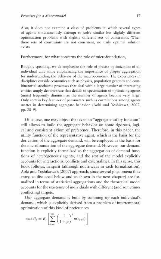
Roughly speaking, we de-emphasize the role of precise optimization of anindividual unit while emphasizing the importance of proper aggregationfor understanding the behavior of the macroeconomy. The experiences indisciplines outside economics such as physics, population genetics and com-binatorial stochastic processes that deal with a large number of interactingentities amply demonstrate that details of specification of optimizing agents(units) frequently diminish as the number of agents become very large.Only certain key features of parameters such as correlations among agentsmatter in determining aggregate behavior. (Aoki and Yoshikawa, 2007,pp. 28–9).
Of course, one may object that even an “aggregate utility function”still allows to build the aggregate behavior on some rigorous, logi-cal and consistent axiom of preference. Therefore, in this paper, theutility function of the representative agent, which is the basis for thederivation of the aggregate demand, will be employed as the basis forthe microfoundation of the aggregate demand. However, our demandfunction is explicitly formalized as the aggregation of demand func-tions of heterogeneous agents, and the rest of the model explicitlyaccounts for interactions, conflicts and externalities. In this sense, thisbook follows, in spirit (although not always in each formalization),Aoki and Yoshikawa’s (2007) approach, since several phenomena (likeentry, as discussed below and as shown in the next chapter) are for-malized in terms of statistical aggregations and the theoretical modelaccounts for the existence of individuals with different (and sometimesconflicting) targets.
Our aggregate demand is built by summing up each individual’sdemand, which is explicitly derived from a problem of intertemporaloptimization of this kind of preferences
max Ut = Et
[ ∞∑i=0
(1
1 + ρ
)i
u(ct+i )
]
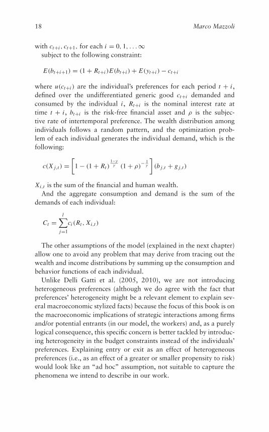
18 Marco Mazzoli
with ct+i , ct+1, for each i = 0, 1, . . .∞subject to the following constraint:
E(bt+i+1) = (1 + Rt+i )E(bt+i ) + E(yt+i ) − ct+i
where u(ct+i ) are the individual’s preferences for each period t + i ,defined over the undifferentiated generic good ct+i demanded andconsumed by the individual i , Rt+i is the nominal interest rate attime t + i , bt+i is the risk-free financial asset and ρ is the subjec-tive rate of intertemporal preference. The wealth distribution amongindividuals follows a random pattern, and the optimization prob-lem of each individual generates the individual demand, which is thefollowing:
c(X j,t ) =[
1 − (1 + Rt )1−γγ (1 + ρ)
− 1γ
](b j,t + g j,t )
Xi,t is the sum of the financial and human wealth.And the aggregate consumption and demand is the sum of the
demands of each individual:
Ct =l∑
j=1
ci (Rt , Xi,t )
The other assumptions of the model (explained in the next chapter)allow one to avoid any problem that may derive from tracing out thewealth and income distributions by summing up the consumption andbehavior functions of each individual.
Unlike Delli Gatti et al. (2005, 2010), we are not introducingheterogeneous preferences (although we do agree with the fact thatpreferences’ heterogeneity might be a relevant element to explain sev-eral macroeconomic stylized facts) because the focus of this book is onthe macroeconomic implications of strategic interactions among firmsand/or potential entrants (in our model, the workers) and, as a purelylogical consequence, this specific concern is better tackled by introduc-ing heterogeneity in the budget constraints instead of the individuals’preferences. Explaining entry or exit as an effect of heterogeneouspreferences (i.e., as an effect of a greater or smaller propensity to risk)would look like an “ad hoc” assumption, not suitable to capture thephenomena we intend to describe in our work.
Premises for a Macromodel 19
1.2.2 Market Structure
The DSGE framework originally departed from the Real BusinessCycle models by introducing some nominal rigidities and monopo-listic competition, i.e., a market configuration where the effects ofentry/exit are not explicitly modeled and the producers of differen-tiated goods are formalized as a continuum of firms in the normalizedspace [0, 1].1
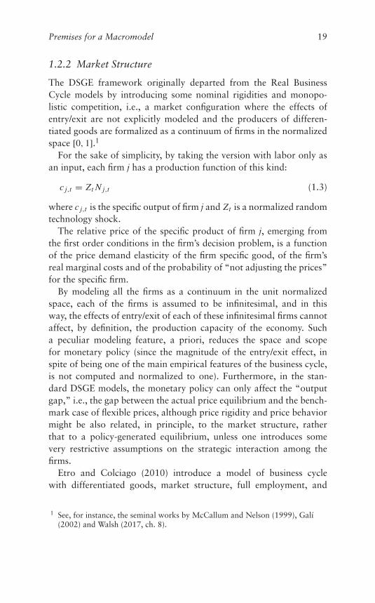
For the sake of simplicity, by taking the version with labor only asan input, each firm j has a production function of this kind:
c j,t = Zt N j,t (1.3)
where c j,t is the specific output of firm j and Zt is a normalized randomtechnology shock.
The relative price of the specific product of firm j, emerging fromthe first order conditions in the firm’s decision problem, is a functionof the price demand elasticity of the firm specific good, of the firm’sreal marginal costs and of the probability of “not adjusting the prices”for the specific firm.
By modeling all the firms as a continuum in the unit normalizedspace, each of the firms is assumed to be infinitesimal, and in thisway, the effects of entry/exit of each of these infinitesimal firms cannotaffect, by definition, the production capacity of the economy. Sucha peculiar modeling feature, a priori, reduces the space and scopefor monetary policy (since the magnitude of the entry/exit effect, inspite of being one of the main empirical features of the business cycle,is not computed and normalized to one). Furthermore, in the stan-dard DSGE models, the monetary policy can only affect the “outputgap,” i.e., the gap between the actual price equilibrium and the bench-mark case of flexible prices, although price rigidity and price behaviormight be also related, in principle, to the market structure, ratherthat to a policy-generated equilibrium, unless one introduces somevery restrictive assumptions on the strategic interaction among thefirms.
Etro and Colciago (2010) introduce a model of business cyclewith differentiated goods, market structure, full employment, and
1 See, for instance, the seminal works by McCallum and Nelson (1999), Galí(2002) and Walsh (2017, ch. 8).
20 Marco Mazzoli
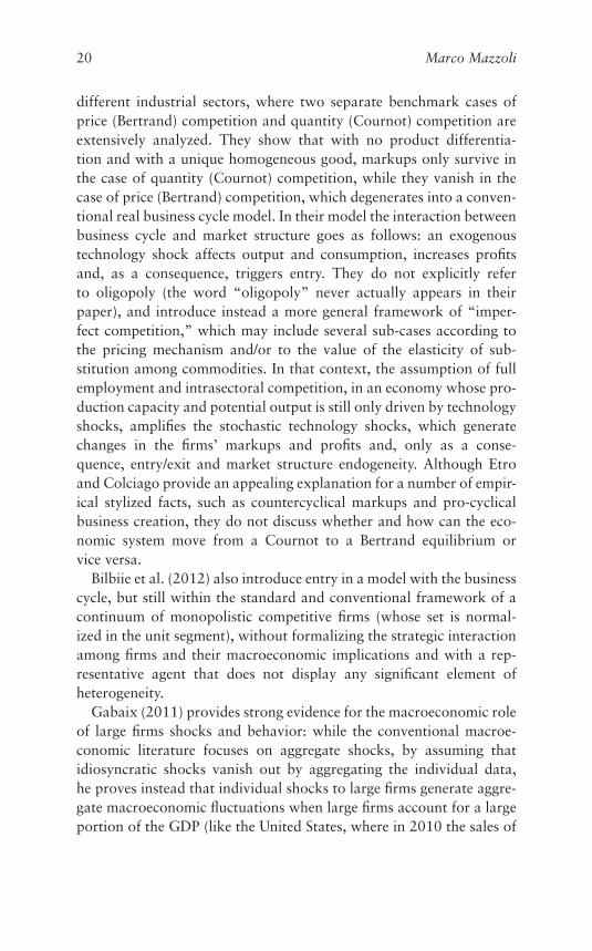
different industrial sectors, where two separate benchmark cases ofprice (Bertrand) competition and quantity (Cournot) competition areextensively analyzed. They show that with no product differentia-tion and with a unique homogeneous good, markups only survive inthe case of quantity (Cournot) competition, while they vanish in thecase of price (Bertrand) competition, which degenerates into a conven-tional real business cycle model. In their model the interaction betweenbusiness cycle and market structure goes as follows: an exogenoustechnology shock affects output and consumption, increases profitsand, as a consequence, triggers entry. They do not explicitly referto oligopoly (the word “oligopoly” never actually appears in theirpaper), and introduce instead a more general framework of “imper-fect competition,” which may include several sub-cases according tothe pricing mechanism and/or to the value of the elasticity of sub-stitution among commodities. In that context, the assumption of fullemployment and intrasectoral competition, in an economy whose pro-duction capacity and potential output is still only driven by technologyshocks, amplifies the stochastic technology shocks, which generatechanges in the firms’ markups and profits and, only as a conse-quence, entry/exit and market structure endogeneity. Although Etroand Colciago provide an appealing explanation for a number of empir-ical stylized facts, such as countercyclical markups and pro-cyclicalbusiness creation, they do not discuss whether and how can the eco-nomic system move from a Cournot to a Bertrand equilibrium orvice versa.
Bilbiie et al. (2012) also introduce entry in a model with the businesscycle, but still within the standard and conventional framework of acontinuum of monopolistic competitive firms (whose set is normal-ized in the unit segment), without formalizing the strategic interactionamong firms and their macroeconomic implications and with a rep-resentative agent that does not display any significant element ofheterogeneity.
Gabaix (2011) provides strong evidence for the macroeconomic roleof large firms shocks and behavior: while the conventional macroe-conomic literature focuses on aggregate shocks, by assuming thatidiosyncratic shocks vanish out by aggregating the individual data,he proves instead that individual shocks to large firms generate aggre-gate macroeconomic fluctuations when large firms account for a largeportion of the GDP (like the United States, where in 2010 the sales of

Premises for a Macromodel 21
the top 100 firms represented 29% of the GDP). He also shows thatshocks on large firms output and behavior explain up to one-third ofSolow residuals and generate a significant share of aggregate outputvariance. This result, called by Gabaix “granular” hypothesis (sincea relevant portion of output can be associated with “large grains” ofeconomic activity), turns out to be particularly significant when thedistribution of firm size is fat-tailed, as empirically documented byGabaix for the US economy. A fat-tailed statistical distribution forfirm size seems to exist not only for the United States, but for manycountries and industries, as shown, for instance, by Corbellini et al.(2010) for the Italian manufacturing sectors, whose size is modeled bya “Pareto II” distribution.
Grassi and Carvalho (2015) provide a theoretical model for firmsand new entrant dynamic decisions employed as a basis for aggre-gating individual firms behavior and generalizing Gabaix (2011)contribution. Their calibration, built in a way to match Gabaix (2011)fat tail of firm size distribution, shows that when the number offirms increases, the rate at which aggregate volatility decays is slowerthan what a central limit argument would predict (i.e., volatility dis-plays a stronger persistence that does not disappear with aggregationif large firms occupy a large market share). Acemoglu et al. (2012)look inside the “black box” of the transmission of the firms idiosyn-cratic shocks from an individual level to a macroeconomic level byproviding a theory of intersectoral input-output linkages entirely con-sistent with Gabaix (2011) findings. Carvalho and Gabaix (2013)provide a similar kind of result by showing a strong evidence tointerpret the data of the US and other four major economies duringthe “great moderation” and its end with a model that again asso-ciates the macroeconomic fluctuations to microeconomic idiosyncraticshocks.
Moreover, our purpose to formalize entry and exit within a macro-model by explicitly endogenizing the market structure requires achange of perspective from the empirical literature in industrial orga-nization and, more in general, from the empirical literature on firmssize for several reasons. First of all, the just mentioned class of mod-els is focused on productivity shocks or technology shocks, while ourwork is focused on another nature of shocks, determined by the strate-gic interactions among oligopolistic firms in an oligopolistic economy.Secondly, we are ideally proposing a general theory and framework

22 Marco Mazzoli
for a macromodel with endogenous market structure that may beadapted to account for specific empirical contexts by introducingspecific assumption for detailed contexts.
Entry decisions are, in general, modeled as the outcome of strate-gic interactions among incumbent and potential entrants, describedby game-theoretical models. Aguirregabiria and Mira (2007) pro-vide a method of sequential estimation of dynamic discrete gamesof incomplete information and introduce, for this purpose, a classof estimators that they call “pseudo maximum likelihood” (PML)estimators, for which they analyze the asymptotic and finite sampleproperties. For the sake of our theoretical macromodel with endoge-nous market structure, the use of some specific statistical properties ofentry and exit would entail some loss of generality: as Sutton (1998)pointed out, while commenting the results of two decades of Indus-trial Organization research, the majority of the results emerging inthe game-theoretic literature were critically relying on some specific, ifnot arbitrary, model assumptions introduced by researchers. Lookingat specific issues, Sutton (2002) analyzes the link between the firm’ssize and its growth rate and, in order to interpret the fact that largefirms do not seem to be much more stable than small firms, he intro-duces a model that he calls “partition of integers.” This model isfurther extended in Sutton (2003), while Sutton (2007), investigatesthe duration of industry leadership and reports an empirical relation-ship between a firm’s current market share and the standard deviationof market share changes by using a Japanese set of 45 industries for23 years.
A methodologically interesting example of agent based simulationin an oligopolistic market is provided by Weidlich and Veit (2008)analysis of the German electricity market, based on the assumptionthat markets should be designed by means of engineering tools, suchas experimentation and computation, instead of statistical assump-tions. In their framework, agent-based modeling methodology offersthe flexibility suitable to specify complex scenarios for market analysisand decision making.
The specificity of these empirical analyses and results, extremelyrelevant for the research shows in any case a different perspectivefrom the one of this book, focused, as we said, on the construction of ageneral macroeconomic framework with endogenous market structurerather than firms’ size statistical analysis.
Premises for a Macromodel 23
1.2.3 Expectations and Implications for the Simulations
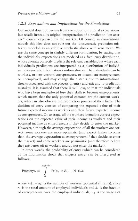
Our model does not deviate from the notion of rational expectations,but recalls instead its original interpretation of a prediction “on aver-age” correct expressed by the market. Of course, in conventionalmodels this idea does not rule out the idiosyncratic prediction mis-takes, modeled as an additive stochastic shock with zero mean. Weuse the same concept in slightly different formulation, by stating thatthe individuals’ expectations are modeled as a frequency distribution,whose average correctly predicts the relevant variables, but where eachindividual’s predictions are interpreted as a distribution of individ-ual idiosyncratic information random shocks. The individuals can beworkers, or new entrant entrepreneurs, or incumbent entrepreneurs,or unemployed, and may change their status due to informationalshocks associated with the process of entry and exit and to predictionmistakes. It is assumed that there is skill loss, so that the individualswho have been unemployed lose their skills to become entrepreneurs,which means that the only potential entrants are the current work-ers, who can also observe the production process of their firms. Thedecision of entry consists of comparing the expected value of theirfuture expected income as workers and their future expected incomeas entrepreneurs. On average, all the workers formulate correct expec-tations on the expected value of their income as workers and theirpotential income as entrepreneurs if they decide to enter the market.However, although the average expectation of all the workers are cor-rect, some workers are more optimistic (and expect higher incomesthan the average expectation as entrepreneurs if they decide to enterthe market) and some workers are pessimistic (and therefore believethey are better off as workers and do not enter the market).
In other words, the probability of entry (which can be consideredas the information shock that triggers entry) can be interpreted asfollows:
Pr(entry)t =nt (1−ht )∫
0
Pr(wt < Et−1,i (t ))i di
where nt (1 − ht ) is the number of workers (potential entrants), sincent is the total amount of employed individuals and ht is the fractionof entrepreneurs over the employed individuals; wt is the wage (set
24 Marco Mazzoli
before the entry decision is taken) and Et−1,i (t ) is the idiosyncraticexpectation of the worker i , in case she decides to enter the market andbecome an entrepreneur. We assume that the expectations expressedby the whole set of workers are correct (and in this sense we do acceptthe notion of rational expectations) but we interpret the expectationsas a frequency distribution.
The way one models expectational shocks carries significant impli-cations for the interpretation of macroeconomic fluctuations. In thispaper, informational shocks on workers’ expectations determine entry,while in conventional models the expectations are associated withthe behavior of the aggregate demand. Lorenzoni (2009) introducesa model of business cycles driven by shocks to consumer expectationsregarding aggregate productivity and where the agents are hit by het-erogeneous productivity shocks: they observe their own productivityand a noisy public signal regarding aggregate productivity, and these“noise shocks,” mimic the features of aggregate demand shocks. Newsshocks (together with other shocks) are the focus of Jaimovich andRebelo (2009) model, which generates both aggregate and sectorialco-movement in response to both contemporaneous shocks and newsshocks about fundamentals.
The issue of interaction between market structure and entry/exitdecisions lead by the agents’ expectations in a macromodel is not anexclusive concern of large industries and large firms. For instance,Dunne et al. (2013) empirically analyze the short-run and long-rundynamics of an oligopolistic sector and the role of entry costs andtoughness of short-run price competition, by using micro data forthe US dentists and chiropractors industries, certainly not two sectorscharacterized by giant firms.
The modeling features are discussed in detail in the next chapter;however, it may be useful to anticipate and introduce a few points inthe present discussion.
The aggregate demand is microfounded and explicitly modeled asthe sum of the individual demand functions. The way the aggregatedemand is formulated allows to account (although in a simplified way)for the wealth distribution and income distribution among workers,incumbent entrepreneurs, new entrant entrepreneurs and unemployed.As shown in the next chapter, this specific modeling feature derivesfrom assuming that the agents are heterogeneous in their budgetconstraints.
Premises for a Macromodel 25
The number of workers, entrepreneur or unemployed individu-als is logically connected to the process of entry/exit, determined byinformation shocks and may potentially generate (as a consequence)distributional shocks on the aggregate demand. In the model it isassumed that the workers are potential entrants and are perceivedas such by the incumbent entrepreneurs; this generates an interactionbetween the labor market equilibrium and the entry/exit decisions.This last assumption aims at characterizing our model as a generalequilibrium model unless we had a price frequency distribution (withdifferent prices set by different oligopolistic firms.) In this sense, sincethe law of one price does not applies to our model, on the one handwe avoid to a great deal the typical DSGE problem of not having aunidirectional causal structure within the period (and ambiguity ofevents time ordering), since in DSGE the endogenous variables are thesolution of a system of simultaneous equations. On the other hand,the very nature of our microfoundation, with heterogeneous agentsin their budget constraints and the assumption that agents’ expecta-tions are modeled as a distribution whose mean corresponds to therational expectations, is clearly more consistent with an agent basedcomputational economics approach than with numerical equationssimulations. This is what we are going to do, after introducing in detailthe theoretical model, in the next chapter.

2 Industrial Structure and theMacroeconomy: The MacroeconomicModel and Its Algebraic Framework
MARCO MAZZOLI1
2.1 Introduction
The previous chapter introduced the rationale and premises for thetheoretical model of this book, which is based on the idea thatin a world of large corporations, with economies characterized byoligopolistic industries, the equilibrium emerging among oligopolis-tic firms may carry significant macroeconomic implications. The birthand death of firms are some of the most relevant empirical phenomenain the business cycle, and our model is microfounding the strate-gic interactions among the firms in a macroeconomic system witholigopolistic features, without referring to the simplifying assumptionsof monopolistic competition that characterize most DSGE models. Tothe extent that very large firms play a relevant role in an oligopolisticeconomic system, not modeling their interactions would leave asidea big part of the story, ignoring causal links between the industrialstructure and the macroeconomy.
The interdependence between the sectorial rates of entry and exitis a well-established empirical fact in the applied research on industrydynamics, as shown by Manjón-Antolín (2010), among others, andthis model provides a general theoretical framework where the inter-dependence between entry and exit is a sub-case that may be repro-duced and traced out in a microfounded macroeconomic context.
The model introduced here plugs the entry/exit decisions into amacroeconomic system by using a notion of statistical distribution ofexpectations that is consistent with the idea of rational expectations
1 I would like to dedicate this chapter to the memory of Prof. Keith Cowling(1936–2016), a long-standing economist at the University of Warwick. Hiscourse “Industrial Structure and the Macroeconomy” has been a great sourceof inspiration for many PhD students of my generation at Warwick. It has beena great privilege and honor for me to be one of them.
26
The Macroeconomic Model and Its Algebraic Framework 27
(at least in its original formulation) to model the entry decision ofpotential entrants. The theoretical framework that we are going tointroduce is also useful for analyzing, on a theoretical ground, thebehavior of firms’ markups over the cycle and is employed for theagent-based simulations contained in the chapters that follow. In par-ticular, we model a macroeconomic system with oligopoly, entry/exitand heterogeneous individuals.
The individuals are heterogeneous in their budget constraints:they can be workers, or new entrant entrepreneurs, or incumbententrepreneurs or unemployed and may change their status due toinformational shocks associated with the process of entry and exit andwith prediction mistakes. The aggregate demand is microfounded andexplicitly modeled as the sum of the individual demands. Divergingincentives between oligopolistic firms and heterogeneous agents arealso explicitly modeled: in particular, entry is determined by infor-mational shocks randomly affecting some workers. Entry and exitrespectively generate or eliminate new entrepreneurs who have tohire workers in order to produce and are therefore associated witha change in the social status of the individuals. In this sense the modelprovides a theoretical interpretation of the links among entry/exit,social mobility and the macroeconomy.
This is rendered by a particular modeling feature, consisting of thefact that the labor market interacts with the process of entry/exit, sincethe latter has the obvious consequence of determining the numberof employed people (number of existing firms hiring workers) and,consequently, macroeconomic fluctuations.
The aggregate demand is explicitly determined by the sum ofindividual demand functions, and also explicitly takes into account(although in a simplified way) the distribution of financial wealth,since the agents are heterogeneous in their budget constraints.
The number of workers, entrepreneurs or unemployed individu-als is logically connected to the process of entry/exit, determined byinformation shocks and may potentially generate (as a consequence)distributional shocks on the aggregate demand. In this regard, it isassumed that the workers are potential entrants and are perceivedas such by the incumbent entrepreneurs: this generates an interactionbetween the labor market equilibrium and the entry/exit decisions.This last assumption characterizes this model as a general equilibriummodel.
28 Marco Mazzoli
Bertoletti and Etro (2016), in a context of partial equilibrium, pro-vide an approach where, for given technological conditions and forthe three cases of monopolistic competition, where, for given techno-logical conditions and for the three cases of monopolistic competition,both Cournot competition (in quantities) and Bertrand competition (inprices) endogenize some elements of the market structure. Differentlyfrom the contribution by Bertoletti and Etro (2016), we do not providea partial equilibrium analysis and assume that the firms’ decisions andstrategies may determine a macroeconomic impact and obtain feed-back from the macroeconomic equilibrium. Finally, while in Bertolettiand Etro (2016) the Cournot and Bertrand benchmarks are basicallyconsistent with pure strategies equilibria in a game among the exist-ing firms, our Cournot oligopolistic equilibrium in the goods markethas the nature of an equilibrium in mixed strategies, since the pur-pose of our research is to track out the macroeconomic impact of theunpredictable outcome (i.e., stochastic shocks) of the rivalry amongthe oligopolistic firms. In particular, our model explicitly links theCournot and Bertrand equilibria by assuming quantity precommit-ments. The oligopolistic firms produce a homogeneous good, and theindividuals cannot be workers and entrepreneurs at the same time butmay change their status as a consequence of different kinds of stochas-tic shocks. Introducing in a macromodel the assumption of quantity(Cournot) competition might raise the problem of how prices aredetermined without referring to an auctioneer or, equivalently, whatprevents the firms from implementing price undercutting. We solve thisproblem by assuming an oligopolistic industrial sector with quantityprecommitment à la Kreps and Scheinkman (1983), with the modifiedand extended assumptions provided by Madden (1998) We use Mad-den (1998) existence theorem of a Cournot-Nash equilibrium in mixedstrategies to formalize the stochastic nature of the firms’ markups,explained as follows.
2.2 The Algebraic Derivation of the Aggregate Demand
Since we are modeling an economy with an oligopolistic industrial sec-tor, the producers choose a point along the demand curve, and, giventheir outputs and their production decisions, they determine, at thesame time, their profits. The individual demand functions are derivedfrom (and therefore consistent with) the optimizing behavior of theconsumers, and the aggregate demand function is explicitly modeled
The Macroeconomic Model and Its Algebraic Framework 29
as the aggregation of the individual demands as shown in the nextsection.
The banking and financial sector is modeled in a simplified wayor, should we say, with a degree of simplification (in particular, theway banking and financial intermediaries are modeled) broadly corre-sponding to the first-generation DSGE models, such as represented byGalí (2008) or Walsh (2017, ch. 8).
The nominal variable At at time t , here defined as “financial assets,”does not include the firm ownership, and, for the sake of simplicity, itis assumed to be risk free. It includes government bonds and deposits(i.e., it corresponds to M3). We also assume that deposits are remu-nerated and that the interest rate on risk-free government bonds isequal to the interest rate on deposits, since they are both assumedto be risk-free financial assets. The monetary policy consists of inter-est rate setting. Exogenous changes in the money stock can be easilyformalized as changes in the nominal amount of risk-free financialassets, since M3 is a function of the money base, but they will notbe considered in this work. Since the focus of this model is not onthe financial sector of the economy, in order to simplify the algebra,we may assume that the banking sector instantaneously performs allthe transactions among individuals, with no specific need for cash.The banking system charges the transactions concerning all the indi-viduals’ incomes (excepting the transactions concerning consumptionof the unemployed individuals, performed by spending the lump-sumtax that covers all the unemployment subsidies) a transaction, feeς . ς is a constant portion of all the transactions, and its magnitudeis extremely small compared to all the other parameters and variablesof the model. These transaction fees (that may also be interpreted asbanking commissions) represent the cost of banks’ intermediation and,in this model with a perfectly competitive banking and financial sector,determine the income of the banking and financial sector, so that theinterest rate on bank lending at time t is equal to the nominal interestrate Rt (rt in real terms) on the asset At , exogenously controlled by thepolicy makers. The banking sector perfectly diversifies its lending riskto the firms, and any risk of financial distress is handled by the lenderof last resort, although the monetary authorities are not in the focusof our analysis.
The entrepreneurs can be incumbent, earning at time t+i the incum-bent nominal profits �in
t+i (�in Rt+i in real terms) or new entrants, earning
the new entrant nominal profits �et+i (�eR
t+i in real terms). �et+i , in
30 Marco Mazzoli
general, diverges from �int+i because the new entrants bear some entry
costs (as explained later). All the agents have the same preferences(i.e., their preferences are represented by the same utility function),but their main source of earnings may be divergent and be giveneither by wages, or profits or transferals to the unemployed individu-als, assumed to be financed, for the sake of simplicity, by a nominallump sum τ (τR in real terms).
The entrepreneurs hire the workers for the period going from t tot+1 and pay them the nominal wages Wt . They also pay themselves thesame nominal wage Wt (wt in real terms) and get the residual nominalprofits, so that the remuneration for the entrepreneurs is Wt plus �in
t+iif the entrepreneur is an incumbent or Wt plus �e
t+i if she is a newentrant. When �in
t+i < 0 or �et+i < 0, (or, equivalently, as shown
below �in Rt+i < 0 and �eR
t+i < 0), the incumbent or the new entrant forthe period going from t to t + 1 goes bankrupt (which happens witha probability to be specified later), the entrepreneur and the workersbecome unemployed and, until they are hired again by a new firm,they receive a transferal given by a portion of the total unemploymentsubsidies, entirely financed by a lump-sum tax τ on the incomes ofthe employed individuals. We assume that the labor contract is suchthat each worker receives the nominal wage Wt for the period goingfrom t + i to t + i + 1, for a fixed amount of hours of work. Letl be the total labor force (assumed to be exogenous and constant),nt+i the number of employed individuals at time t + i , hin
t+i (with 0 <
hint+i < ht+i ) the portion of incumbent entrepreneurs at time t + i and
het+i (with 0 < he
t+i < 1) the portion of new entrants at time t + i(with ht+i = hin
t+i + het+i and 0 < ht+i < ht+i ). This means that the
portion of workers over the total employed labor force is given by1 − hin
t+i − het+i = 1 − ht+i .
(nt+i Wt+i + nt+i hint+i�
int+i + nt+i he
t+i�et+i )ς are the transaction fees
to the banking system at time t + i , since each employed individ-ual pays a nominal lump-sum tax τ (τR in real terms) to finance theunemployment subsidies. nt+iτR(1 − ς) is the overall amount of realunemployment subsidies (net of the transaction fees to the bankingsystem). We assume that τR and ς are constant and very small in theirmagnitude, so that τR is assumed to barely cover the survival expensesof the unemployed individuals.
The model displays a form of skill loss: being an entrepreneurrequires some skills that are lost by not working and being
The Macroeconomic Model and Its Algebraic Framework 31
unemployed for one period or more. On the other hand, being aworker is not assumed to require any particular skill. On the basisof our assumptions, we may simplify out the effects of tax transfer-als and bank commissions and formalize the aggregate demand asfollows:
Yt+i = nt+i (Wt+i + hint+i�
int+i + he
t+i�et+i − τ)(1 − ς)+
+ nt+iτ(1 − ς) + nt+i (Wt+i + hint+i�
int+i + he
t+i�et+i )ς
Yt+i = nt+i (Wt+i + hint+i�
int+i + he
t+i�et+i ) (2.1)
What is needed, for the sake of our model, is a proper formalizationof an aggregate demand function, and we model it in such a way thatit is explicitly formalized as the aggregation of the individual demandsexpressed by each consumer. We also explicitly show that such indi-vidual demands are consistent with (and therefore derived from) theoptimizing behavior of the consumers.
We derive and microfound the aggregate demand in a rather con-ventional way, based on a standard optimization problem of theconsumer. Given the overall forward-looking preferences U j,t for thegeneric consumer j , and defining the utility in each period t as u(c j,t ),a function of the amount of goods consumed for time t , we can nowturn to the individual consumer problem, which is very similar to theone presented in (Bagliano and Bertola, 2004, ch.1). Its purpose is todefine a microfounded aggregate demand, explicitly formalized as theaggregation of the individual demand functions of each consumer. Letus assume that the preferences of the individuals are represented by aCRRA utility function and the consumer problem is formalized as astandard intertemporal optimization problem:
max Ut = Et
[ ∞∑i=0
(1
1 + ρ
)i
u(c j,t+i )
](2.2)
c j,t+i , i = 0, 1, . . . ,∞ (2.3)
subject to the following constraint, where, as usual for the dynamicmodels, the interest rate is introduced in nominal terms,
E(b j,t+i+1) = (1 + Rt+i )E(b j,t+i ) + E(y j,t+i ) − c j,t+i (2.4)
32 Marco Mazzoli
and
c j,t+i ≥ 0
at every time t + i from i = 0, 1, . . . ,∞, where:
●
(1
1+ρ
)is the subjective discount factor;
● Rt is the nominal interest rate on the financial asset at time t(controlled by the central bank);
● c j,t is the real consumption at time t for the consumers (defined asc j,t = C j,t/Pt , with C j,t as the nominal consumption and Pt as theprice level at time t);
● y j,t is the consumer j ’s real income (defined as y j,t = Y j,t/Pt , whereY j,t is the nominal income at time t) and b j,t is the real financialwealth held by the individual consumer j at time t (again defined asb j,t = B j,t/Pt , with B j,t as the nominal financial wealth at time t),which may be defined as a random portion δ j of the aggregate realwealth a j,t (i.e., b j,t = δ j a j,t with 0 < δ j < 1), so that summing upto all the l individuals, we have
∑j δ j a j,t = a j,t and
∑j δ j = 1.
The price level Pt at time t is, of course, a macroeconomic variable alsoallowing one to determine the link between nominal and real variablesand is the average of the frequency distribution of all the prices set bythe oligopolistic firms.
The financial assets are risk free and do not include shares: in thissimplified model, investing in shares is a time-consuming activity andimplies being an entrepreneur. The budget constraint (2.4) also holdsfor any time i = 0, 1, . . . ,∞. The transversality condition is as follows:
limj−→∞ bt+ j
(1
1 + Rt+ j
) j
≥ 0
Since the marginal utility of consumption is always positive, thetransversality condition is always satisfied in terms of equality. Thefinancial wealth b j,t and the individual human capital (let us defineit g j,t ) are assumed to be valued at the beginning of period t , whileX j,t = (1 + Rt )(b j,t + g j,t ) represents the individual total wealth,which is valued at the end of period t , but before consumption c j,t ,that absorbs part of the available resources. We also assume that bothprofits and wages are paid at the end of the period, when consumptiontakes place. The human capital valued at the beginning of time t is
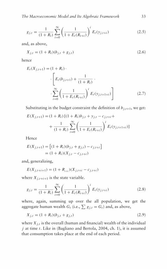
The Macroeconomic Model and Its Algebraic Framework 33
g j,t = 1
(1 + Rt )
∞∑i=0
(1
1 + Et (Rt+i )
)i
Et (y j,t+i ) (2.5)
and, as above,
X j,t = (1 + Rt )(b j,t + g j,t ) (2.6)
hence
Et (X j,t+1) = (1 + Rt ) ·
·[
Et (b j,t+1) + 1
(1 + Rt )·
·∞∑
i=0
(1
1 + Et (Rt+i )
)i
Et (y j,t+1+i )
](2.7)
Substituting in the budget constraint the definition of b j,t+1, we get:
E(X j,t+1) = (1 + Rt ) [(1 + Rt )b j,t + y j,t − c j,t+i+
+ 1
(1 + Rt )
∞∑i=0
(1
1 + Et (Rt+i )
)i
Et (y j,t+1+i )]
Hence
E(X j,t+1) = [(1 + Rt )(b j,t + g j,t ) − c j,t+i
]= (1 + Rt )(X j,t − c j,t+i )
and, generalizing,
E(X j,t+i+1) = (1 + Rt+i )(X j,t+i − c j,t+i )
where X j,t+i+1 is the state variable.
g j,t = 1
(1 + Rt )
∞∑i=0
(1
1 + Et (Rt+i )
)i
Et (y j,t+i ) (2.8)
where, again, summing up over the all population, we get theaggregate human wealth Gt (i.e.,
∑g j,t = Gt ) and, as above,
X j,t = (1 + Rt )(b j,t + g j,t ) (2.9)
where X j,t is the overall (human and financial) wealth of the individualj at time t . Like in (Bagliano and Bertola, 2004, ch. 1), it is assumedthat consumption takes place at the end of each period.
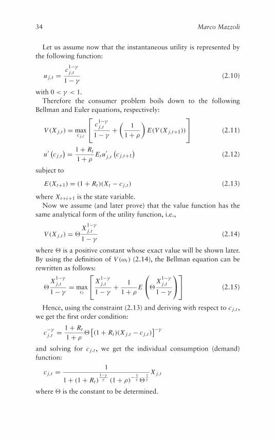
34 Marco Mazzoli
Let us assume now that the instantaneous utility is represented bythe following function:
u j,t = c1−γ
j,t
1 − γ(2.10)
with 0 < γ < 1.Therefore the consumer problem boils down to the following
Bellman and Euler equations, respectively:
V (X j,t ) = maxc j,t
⎡⎣ c1−γ
j,t
1 − γ+(
1
1 + ρ
)E(V (X j,t+1))
⎤⎦ (2.11)
u′ (c j,t) = 1 + Rt
1 + ρEt u
′j,t
(c j,t+1
)(2.12)
subject to
E(Xt+1) = (1 + Rt )(Xt − c j,t ) (2.13)
where Xt+i+1 is the state variable.Now we assume (and later prove) that the value function has the
same analytical form of the utility function, i.e.,
V (X j,t ) = �X1−γ
j,t
1 − γ(2.14)
where � is a positive constant whose exact value will be shown later.By using the definition of V (ωt ) (2.14), the Bellman equation can berewritten as follows:
�X1−γ
j,t
1 − γ= max
ct
⎡⎣ X1−γ
j,t
1 − γ+ 1
1 + ρE
⎛⎝�X1−γ
j,t
1 − γ
⎞⎠⎤⎦ (2.15)
Hence, using the constraint (2.13) and deriving with respect to c j,t ,we get the first order condition:
c−γ
j,t = 1 + Rt
1 + ρ�[(1 + Rt )(X j,t − c j,t )
]−γ
and solving for c j,t , we get the individual consumption (demand)function:
c j,t = 1
1 + (1 + Rt )1−γγ (1 + ρ)
− 1γ �
1γ
X j,t
where � is the constant to be determined.
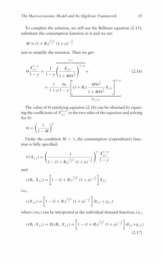
The Macroeconomic Model and Its Algebraic Framework 35
To complete the solution, we still use the Bellman equation (2.15),substitute the consumption function in it and we set:
M ≡ (1 + Rt )1−γγ (1 + ρ)
− 1γ
just to simplify the notation. Then we get:
�X1−γ
j,t
1 − γ= 1
1 − γ
c j,t︷ ︸︸ ︷(X j,t
1 + M�1γ
)1−γ
+ (2.16)
+ 1
1 + ρ
�t
1 − γ
⎡⎣(1 + Rt )M�
1γ
1 + M�1γ
X j,t
⎤⎦1−γ
︸ ︷︷ ︸X j,t+1
The value of � satisfying equation (2.16) can be obtained by equat-ing the coefficients of X1−γ
j,t in the two sides of the equation and solvingfor �:
� =(
1
1 − M
)γ
Under the condition M < 1, the consumption (expenditure) func-tion is fully specified:
V (X j,t ) =(
1
1 − (1 + Rt )1−γγ (1 + ρ)
− 1γ
)γX1−γ
j,t
1 − γ
and
c(Rt , X j,t ) =[
1 − (1 + Rt )1−γγ (1 + ρ)
− 1γ
]X j,t
i.e.,
c(X j,t ) =[
1 − (1 + Rt )1−γγ (1 + ρ)
− 1γ
](b j,t + g j,t )
where c(wt ) can be interpreted as the individual demand function, i.e.,
c(Rt , X j,t ) = Dt (Rt , X j,t ) =[
1 − (1 + Rt )1−γγ (1 + ρ)
− 1γ
](b j,t+g j,t )
(2.17)
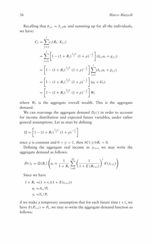
36 Marco Mazzoli
Recalling that b j,t = δ j,t at and summing up for all the individuals,we have:
Ct =l∑
j=1
ci (Rt , Xi,t )
=l∑
i=1
[1 − (1 + Rt )
1−γγ (1 + ρ)
− 1γ
](δi,t at + g j,t )
=[
1 − (1 + Rt )1−γγ (1 + ρ)
− 1γ
] l∑i=1
(δi,t at + g j,t )
=[
1 − (1 + Rt )1−γγ (1 + ρ)
− 1γ
](at + Gt )
=[
1 − (1 + Rt )1−γγ (1 + ρ)
− 1γ
]Wt
where Wt is the aggregate overall wealth. This is the aggregatedemand.
We can rearrange the aggregate demand Dt (·) in order to accountfor income distribution and expected future variables, under rathergeneral assumptions. Let us start by defining
� =[
1 − (1 + Rt )1−γγ (1 + ρ)
− 1γ
]since ρ is constant and 0 < γ < 1, then ∂C(·)/∂Rt < 0.
Defining the aggregate real income as yt+i , we may write theaggregate demand as follows:
D(·)t = �(Rt )
(at + 1
1 + Rt
∞∑i=0
(1
1 + E (Rt+i )
)i
E(yt+i )
)
Since we have
1 + Rt =(1 + rt )(1 + E(ιt+i ))
at =At/Pt
yt =Yt/Pt
if we make a temporary assumption that for each future time t + i , wehave E(Pt+i ) = Pt , we may re-write the aggregate demand function asfollows:
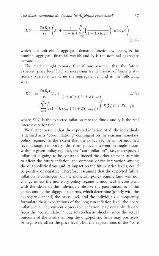
The Macroeconomic Model and Its Algebraic Framework 37
D(·)t = �(Rt )
Pt
(At + 1
(1 + Rt )
∞∑i=0
(1
1 + E (Rt+i )
)i
E(Yt+i )
)(2.18)
which is a unit elastic aggregate demand function, where At is thenominal aggregate financial wealth and Yt is the nominal aggregateincome.
The reader might remark that if one assumed that the futureexpected price level had an increasing trend instead of being a sta-tionary variable, we write the aggregate demand in the followingway:
D(·)t = �(Rt )
Pt(At + 1
(1 + E (rt ))(1 + E(ιt+1))· (2.19)
·∞∑
i=0
(1
(1 + E (rt+i ))(1 + E(ιt+i+1))
)i
E(Yt )(1 + E(ιt+i ))
where E(ιt ) is the expected inflation rate for time t and rt is the realinterest rate for time t.
We further assume that the expected inflation of all the individualsis defined as a “core inflation,” contingent on the existing monetarypolicy regime. To the extent that the policy regime is not modified(even though temporary, short-run policy intervention might occurwithin a given policy regime), the “core inflation” (i.e., the expectedinflation) is going to be constant. Indeed the other element suitableto affect the future inflation, the outcome of the interaction amongthe oligopolistic firms and its impact on the future price levels, couldbe positive or negative. Therefore, assuming that the expected futureinflation is contingent on the monetary policy regime (and will notchange unless the monetary policy regime is modified) is consistentwith the idea that the individuals observe the past outcomes of thegames among the oligopolistic firms, which determine (jointly with theaggregate demand) the price level, and the individuals consequentlyformulate their expectations of the long run inflation level, the “coreinflation” ι. The current observable inflation may certainly deviatefrom the “core inflation” due to stochastic shocks (since the actualoutcome of the rivalry among the oligopolistic firms may positivelyor negatively affect the price level), but the expectations of the “core
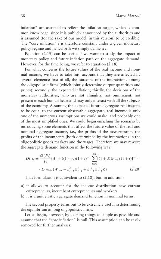
38 Marco Mazzoli
inflation” are assumed to reflect the inflation target, which is com-mon knowledge, since it is publicly announced by the authorities andis assumed (for the sake of our model, in this version) to be credible.The “core inflation” ι is therefore constant under a given monetarypolicy regime and henceforth we simply define it ι.
Equation (2.19) can be useful if we want to study the impact ofmonetary policy and future inflation path on the aggregate demand.However, for the time being, we refer to equation (2.18).
For what concerns the future values of the real income and nom-inal income, we have to take into account that they are affected byseveral elements: first of all, the outcome of the interactions amongthe oligopolistic firms (which jointly determine output quantities andprices); secondly, the expected inflation; thirdly, the decisions of themonetary authorities, who are not almighty, not omniscient, notpresent in each human heart and may only interact with all the subjectsof the economy. Assuming the expected future aggregate real incometo be equal to the current observable aggregate, real income is onlyone of the numerous assumptions we could make, and probably oneof the most simplified ones. We could begin enriching the scenario byintroducing some elements that affect the future value of the real andnominal aggregate income, i.e., the profits of the new entrants, theprofits of the incumbents (both determined by the interactions in theoligopolistic goods market) and the wages. Therefore we may rewritethe aggregate demand function in the following way:
D(·)t = �(Rt )
Pt{At + ((1 + rt )(1 + ι)−1
∞∑i=0
[(1 + E (rt+i ) (1 + ι)]−i ·
· E(nt+i (Wt+i + het+i�
et+i + hin
t+i�int+i ))} (2.20)
That formulation is equivalent to (2.18), but, in addition:
a) it allows to account for the income distribution new entrantentrepreneurs, incumbent entrepreneurs and workers;
b) it is a unit elastic aggregate demand function in nominal terms.
The second property turns out to be extremely useful in determiningthe equilibrium among oligopolistic firms.
Let us begin, however, by keeping things as simple as possible andassume that the “core inflation” is null. This assumption can be easilyremoved for further analyses.
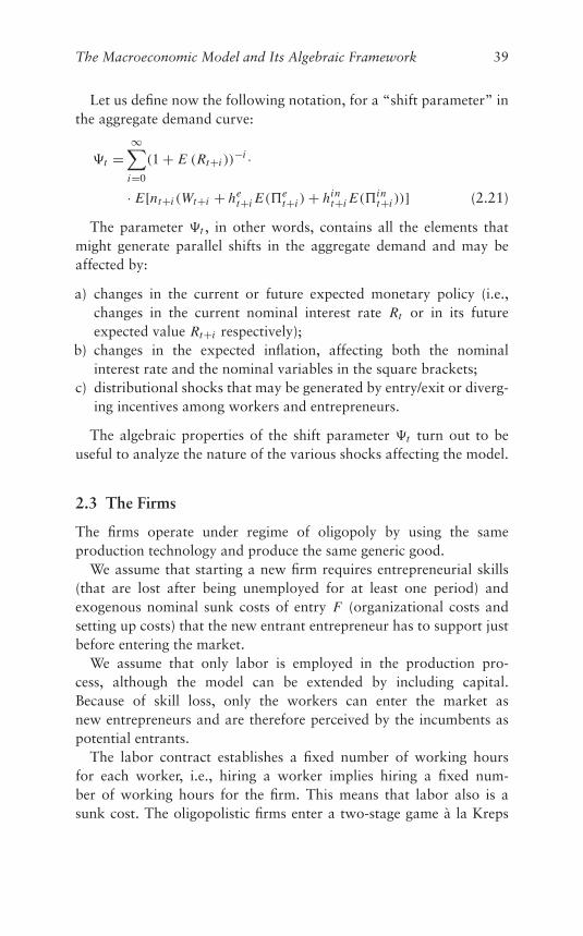
The Macroeconomic Model and Its Algebraic Framework 39
Let us define now the following notation, for a “shift parameter” inthe aggregate demand curve:
�t =∞∑
i=0
(1 + E (Rt+i ))−i ·
· E[nt+i (Wt+i + het+i E(�e
t+i ) + hint+i E(�in
t+i ))] (2.21)
The parameter �t , in other words, contains all the elements thatmight generate parallel shifts in the aggregate demand and may beaffected by:
a) changes in the current or future expected monetary policy (i.e.,changes in the current nominal interest rate Rt or in its futureexpected value Rt+i respectively);
b) changes in the expected inflation, affecting both the nominalinterest rate and the nominal variables in the square brackets;
c) distributional shocks that may be generated by entry/exit or diverg-ing incentives among workers and entrepreneurs.
The algebraic properties of the shift parameter �t turn out to beuseful to analyze the nature of the various shocks affecting the model.
2.3 The Firms
The firms operate under regime of oligopoly by using the sameproduction technology and produce the same generic good.
We assume that starting a new firm requires entrepreneurial skills(that are lost after being unemployed for at least one period) andexogenous nominal sunk costs of entry F (organizational costs andsetting up costs) that the new entrant entrepreneur has to support justbefore entering the market.
We assume that only labor is employed in the production pro-cess, although the model can be extended by including capital.Because of skill loss, only the workers can enter the market asnew entrepreneurs and are therefore perceived by the incumbents aspotential entrants.
The labor contract establishes a fixed number of working hoursfor each worker, i.e., hiring a worker implies hiring a fixed num-ber of working hours for the firm. This means that labor also is asunk cost. The oligopolistic firms enter a two-stage game à la Kreps
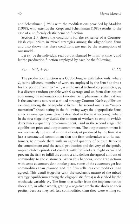
40 Marco Mazzoli
and Scheinkman (1983) with the modifications provided by Madden(1998), who extends the Kreps and Scheinkman (1983) results to thecase of a uniformly elastic demand function.
Section 2.9 shows the conditions for the existence of a Cournot-Nash equilibrium in mixed strategies among the oligopolistic firmsand also shows that these conditions are met by the assumptions ofour model.
Let ϕi,t be the individual real output planned by firm i at time t , andlet the production function employed by each be the following:
ϕi,t = �Lαi,t + ψi,t (2.22)
The production function is a Cobb-Douglas with labor only, whereLt is the (discrete) number of workers employed by the firm i at time tfor the period from t to t + 1, � is the usual technology parameter, ψt
is a discrete random variable with 0 average and uniform distributioncontaining the information on two stochastic phenomena: the first oneis the stochastic nature of a mixed-strategy Cournot-Nash equilibriumexisting among the oligopolistic firms. The second one is an “imple-mentation” shock acting in the following way: the oligopolistic firmsenter a two-stage game (briefly described in the next sections), wherein the first stage they decide the amount of workers to employ (whichdetermines a quantity pre-commitment), and in the second stage, theequilibrium price and output commitment. The output commitment isnot necessarily the actual amount of output produced by the firm: it isjust a contractual commitment that the firm undertakes with its cus-tomers, to provide them with an agreed quantity of output. Betweenthe commitment and the actual production and delivery of the goods,unpredictable episodes of conflict with the workers might occur andprevent the firm to fulfill the contract and deliver the agreed amount ofcommodity to the customers. When this happens, some transactionswith some customers do not take place, some of the customers get lesscommodities than planned and the firm sells less commodities thanagreed. This detail (together with the stochastic nature of the mixedstrategy equilibrium among the oligopolistic firms) is described by thestochastic variable ψt . The firms that suffer from the implementationshock are, in other words, getting a negative stochastic shock to theirprofits, because they sell less commodities than they were willing to.
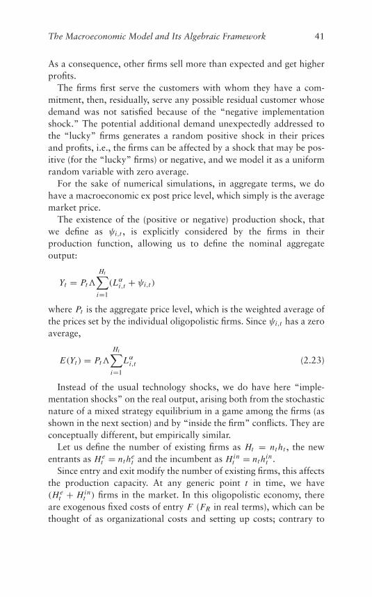
The Macroeconomic Model and Its Algebraic Framework 41
As a consequence, other firms sell more than expected and get higherprofits.
The firms first serve the customers with whom they have a com-mitment, then, residually, serve any possible residual customer whosedemand was not satisfied because of the “negative implementationshock.” The potential additional demand unexpectedly addressed tothe “lucky” firms generates a random positive shock in their pricesand profits, i.e., the firms can be affected by a shock that may be pos-itive (for the “lucky” firms) or negative, and we model it as a uniformrandom variable with zero average.
For the sake of numerical simulations, in aggregate terms, we dohave a macroeconomic ex post price level, which simply is the averagemarket price.
The existence of the (positive or negative) production shock, thatwe define as ψi,t , is explicitly considered by the firms in theirproduction function, allowing us to define the nominal aggregateoutput:
Yt = Pt�
Ht∑i=1
(Lαi,t + ψi,t )
where Pt is the aggregate price level, which is the weighted average ofthe prices set by the individual oligopolistic firms. Since ψi,t has a zeroaverage,
E(Yt ) = Pt�
Ht∑i=1
Lαi,t (2.23)
Instead of the usual technology shocks, we do have here “imple-mentation shocks” on the real output, arising both from the stochasticnature of a mixed strategy equilibrium in a game among the firms (asshown in the next section) and by “inside the firm” conflicts. They areconceptually different, but empirically similar.
Let us define the number of existing firms as Ht = nt ht , the newentrants as He
t = nt het and the incumbent as Hin
t = nt hint .
Since entry and exit modify the number of existing firms, this affectsthe production capacity. At any generic point t in time, we have(He
t + Hint ) firms in the market. In this oligopolistic economy, there
are exogenous fixed costs of entry F (FR in real terms), which can bethought of as organizational costs and setting up costs; contrary to
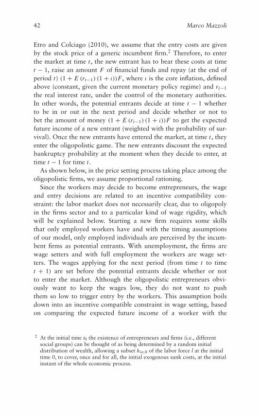
42 Marco Mazzoli
Etro and Colciago (2010), we assume that the entry costs are givenby the stock price of a generic incumbent firm.2 Therefore, to enterthe market at time t , the new entrant has to bear these costs at timet − 1, raise an amount F of financial funds and repay (at the end ofperiod t) (1 + E (rt−1) (1 + ι))F , where ι is the core inflation, definedabove (constant, given the current monetary policy regime) and rt−1
the real interest rate, under the control of the monetary authorities.In other words, the potential entrants decide at time t − 1 whetherto be in or out in the next period and decide whether or not tobet the amount of money (1 + E (rt−1) (1 + ι))F to get the expectedfuture income of a new entrant (weighted with the probability of sur-vival). Once the new entrants have entered the market, at time t , theyenter the oligopolistic game. The new entrants discount the expectedbankruptcy probability at the moment when they decide to enter, attime t − 1 for time t .
As shown below, in the price setting process taking place among theoligopolistic firms, we assume proportional rationing.
Since the workers may decide to become entrepreneurs, the wageand entry decisions are related to an incentive compatibility con-straint: the labor market does not necessarily clear, due to oligopolyin the firms sector and to a particular kind of wage rigidity, whichwill be explained below. Starting a new firm requires some skillsthat only employed workers have and with the timing assumptionsof our model, only employed individuals are perceived by the incum-bent firms as potential entrants. With unemployment, the firms arewage setters and with full employment the workers are wage set-ters. The wages applying for the next period (from time t to timet + 1) are set before the potential entrants decide whether or notto enter the market. Although the oligopolistic entrepreneurs obvi-ously want to keep the wages low, they do not want to pushthem so low to trigger entry by the workers. This assumption boilsdown into an incentive compatible constraint in wage setting, basedon comparing the expected future income of a worker with the
2 At the initial time t0 the existence of entrepreneurs and firms (i.e., differentsocial groups) can be thought of as being determined by a random initialdistribution of wealth, allowing a subset hin,0 of the labor force l at the initialtime 0, to cover, once and for all, the initial exogenous sunk costs, at the initialinstant of the whole economic process.
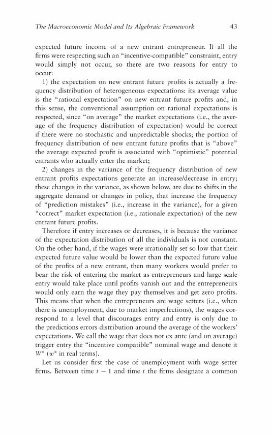
The Macroeconomic Model and Its Algebraic Framework 43
expected future income of a new entrant entrepreneur. If all thefirms were respecting such an “incentive-compatible” constraint, entrywould simply not occur, so there are two reasons for entry tooccur:
1) the expectation on new entrant future profits is actually a fre-quency distribution of heterogeneous expectations: its average valueis the “rational expectation” on new entrant future profits and, inthis sense, the conventional assumption on rational expectations isrespected, since “on average” the market expectations (i.e., the aver-age of the frequency distribution of expectation) would be correctif there were no stochastic and unpredictable shocks; the portion offrequency distribution of new entrant future profits that is “above”the average expected profit is associated with “optimistic” potentialentrants who actually enter the market;
2) changes in the variance of the frequency distribution of newentrant profits expectations generate an increase/decrease in entry;these changes in the variance, as shown below, are due to shifts in theaggregate demand or changes in policy, that increase the frequencyof “prediction mistakes” (i.e., increase in the variance), for a given“correct” market expectation (i.e., rationale expectation) of the newentrant future profits.
Therefore if entry increases or decreases, it is because the varianceof the expectation distribution of all the individuals is not constant.On the other hand, if the wages were irrationally set so low that theirexpected future value would be lower than the expected future valueof the profits of a new entrant, then many workers would prefer tobear the risk of entering the market as entrepreneurs and large scaleentry would take place until profits vanish out and the entrepreneurswould only earn the wage they pay themselves and get zero profits.This means that when the entrepreneurs are wage setters (i.e., whenthere is unemployment, due to market imperfections), the wages cor-respond to a level that discourages entry and entry is only due tothe predictions errors distribution around the average of the workers’expectations. We call the wage that does not ex ante (and on average)trigger entry the “incentive compatible” nominal wage and denote itW ∗ (w∗ in real terms).
Let us consider first the case of unemployment with wage setterfirms. Between time t − 1 and time t the firms designate a common
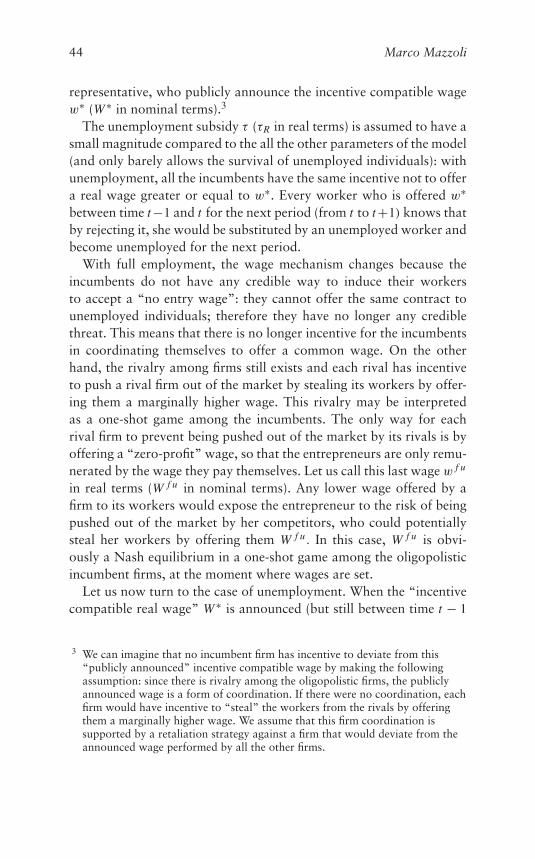
44 Marco Mazzoli
representative, who publicly announce the incentive compatible wagew∗ (W ∗ in nominal terms).3
The unemployment subsidy τ (τR in real terms) is assumed to have asmall magnitude compared to the all the other parameters of the model(and only barely allows the survival of unemployed individuals): withunemployment, all the incumbents have the same incentive not to offera real wage greater or equal to w∗. Every worker who is offered w∗between time t−1 and t for the next period (from t to t+1) knows thatby rejecting it, she would be substituted by an unemployed worker andbecome unemployed for the next period.
With full employment, the wage mechanism changes because theincumbents do not have any credible way to induce their workersto accept a “no entry wage”: they cannot offer the same contract tounemployed individuals; therefore they have no longer any crediblethreat. This means that there is no longer incentive for the incumbentsin coordinating themselves to offer a common wage. On the otherhand, the rivalry among firms still exists and each rival has incentiveto push a rival firm out of the market by stealing its workers by offer-ing them a marginally higher wage. This rivalry may be interpretedas a one-shot game among the incumbents. The only way for eachrival firm to prevent being pushed out of the market by its rivals is byoffering a “zero-profit” wage, so that the entrepreneurs are only remu-nerated by the wage they pay themselves. Let us call this last wage w f u
in real terms (W f u in nominal terms). Any lower wage offered by afirm to its workers would expose the entrepreneur to the risk of beingpushed out of the market by her competitors, who could potentiallysteal her workers by offering them W f u . In this case, W f u is obvi-ously a Nash equilibrium in a one-shot game among the oligopolisticincumbent firms, at the moment where wages are set.
Let us now turn to the case of unemployment. When the “incentivecompatible real wage” W ∗ is announced (but still between time t − 1
3 We can imagine that no incumbent firm has incentive to deviate from this“publicly announced” incentive compatible wage by making the followingassumption: since there is rivalry among the oligopolistic firms, the publiclyannounced wage is a form of coordination. If there were no coordination, eachfirm would have incentive to “steal” the workers from the rivals by offeringthem a marginally higher wage. We assume that this firm coordination issupported by a retaliation strategy against a firm that would deviate from theannounced wage performed by all the other firms.

The Macroeconomic Model and Its Algebraic Framework 45
and time t), some employed workers may be affected by an “opti-mistic” idiosyncratic informational shock that make them decide toenter the market. Entry/exit affect the number of existing firms, andhence production capacity and aggregate employment.
The risk-free interest rate Rt is exogenous and under the control ofthe monetary authorities, and the revenue of the perfectly competitivebanking and financial system is determined by the transaction fees andnot by any interest margin; therefore Rt is also the interest rate thatthe firms have to pay to the banks on their loans.
In case of bankruptcy, the entrepreneurs lose their job, do not havethe right to start a new firm next period, but keep their free financialassets At . This means, in aggregate terms, that it is irrelevant who isactually holding the financial assets At . Since any new firm has limitedliability (and is a distinguished entity from the entrepreneur), any newentrant borrows from the banking and financial system in order tocover the cost of entry.
The expected remuneration of the entrepreneur is given by the prof-its (�e
t if it is a new entrant, �int if it is an incumbent) plus the wage
W ∗t that the entrepreneur pays to herself.The expected real payoff of the new entrant at time t − 1 for time
t , (Et−1(�eRt ) + w∗
t − τR − (1 + ι)(1 + rt−1)FR) (1 − ς)), is different,in general, from the expected real remuneration of the incumbent,(Et−1(�
in Rt ) + w∗
t − τR) (1 − ς)).Since entry and exit are determined by information shocks, with no
modifications in the entry costs and for a given level of interest rate Rt ,the survival of new entrants depends on their ability to substitute thefirms that abandon the market, or by new equilibria configurations inthe (oligopolistic) market for goods.
Having defined earlier the individual real output of the oligopolisticfirm i at time t +1 as ϕi,t+1, in equilibrium ϕi,t+1 and L∗
t+1, the amountof labor employed by firm i (which also determines the quantity pre-commitment among the oligopolistic firms) depends on the outcomeof the game among the oligopolistic firms.
Since entry and exit are determined by information shocks, ceterisparibus (with no modifications in the entry costs and for a givenlevel of interest rate rt and a given “core inflation” rate ιt ), the sur-vival of new entrants depends on their ability to substitute the firmsthat abandon the market, or by new equilibria configurations in the(oligopolistic) market for goods.
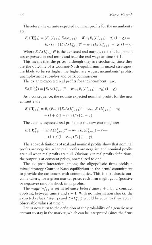
46 Marco Mazzoli
Therefore, the ex ante expected nominal profits for the incumbent iare:
Et (�int+1) = [Et (Pt+1) Et (ϕi,t+1) − Wt+1 Et (L
∗i,t+1) − τ ] (1 − ς) =
= Et (Pt+1) [Et�(L∗i,t+1)
α − wt+1 Et (L∗i,t+1) − τR] (1 − ς)
Where Et�(L∗i,t+1)
α is the expected real output, τR is the lump-sumtax expressed in real terms and wt+1the real wage at time t + 1.
This means that the prices (although they are stochastic, since theyare the outcome of a Cournot-Nash equilibrium in mixed strategies)are likely to be set higher the higher are wages, incumbents’ profits,unemployment subsidies and bank commissions.
The ex ante expected real profits for the incumbent i are:
Et (�in Rt+1) = [Et�(L∗
i,t+1)α − wt+1 Et (L
∗i,t+1) − τR] (1 − ς)
As a consequence, the ex ante expected nominal profits for the newentrant j are:
Et (�et+1) = Et (Pt+1) [Et�(L∗
j,t+1)α − wt+1 Et (L
∗j,t+1) − τR−
− (1 + ι)(1 + rt−1)FR] (1 − ς)
The ex ante expected real profits for the new entrant j are:
Et (�eRt+1) = [Et�(L∗
j,t+1)α − wt+1 Et (L
∗j,t+1) − τR−
− (1 + ι)(1 + rt−1)FR] (1 − ς)
The above definitions of real and nominal profits show that nominalprofits are negative when real profits are negative and nominal profitsare null when real profits are null. Obviously in real profits definitions,the output is at constant prices, normalized to one.
The ex post interaction among the oligopolistic firms yields amixed-strategy Cournot-Nash equilibrium in the firms’ commitmentto provide the customers with commodities. This is a stochastic out-come where, for a given market price, each firm might get a (positiveor negative) random shock in its profits.
The wage W ∗t+1 is set in advance before time t + 1 by a contract
applying between time t and t + 1. With no information shocks, theexpected values Et (ϕt+1) and Et (L∗
t+1) would be equal to their actualobservable values at time t .
Let us now turn to the definition of the probability of a generic newentrant to stay in the market, which can be interpreted (since the firms
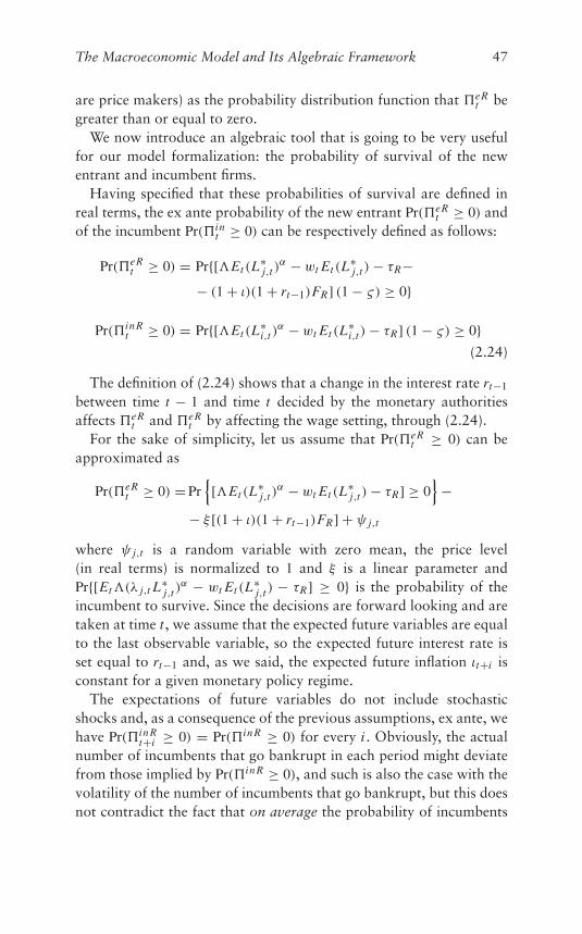
The Macroeconomic Model and Its Algebraic Framework 47
are price makers) as the probability distribution function that �eRt be
greater than or equal to zero.We now introduce an algebraic tool that is going to be very useful
for our model formalization: the probability of survival of the newentrant and incumbent firms.
Having specified that these probabilities of survival are defined inreal terms, the ex ante probability of the new entrant Pr(�eR
t ≥ 0) andof the incumbent Pr(�in
t ≥ 0) can be respectively defined as follows:
Pr(�eRt ≥ 0) = Pr{[�Et (L
∗j,t )
α − wt Et (L∗j,t ) − τR−
− (1 + ι)(1 + rt−1)FR] (1 − ς) ≥ 0}
Pr(�in Rt ≥ 0) = Pr{[�Et (L
∗i,t )
α − wt Et (L∗i,t ) − τR] (1 − ς) ≥ 0}
(2.24)
The definition of (2.24) shows that a change in the interest rate rt−1
between time t − 1 and time t decided by the monetary authoritiesaffects �eR
t and �eRt by affecting the wage setting, through (2.24).
For the sake of simplicity, let us assume that Pr(�eRt ≥ 0) can be
approximated as
Pr(�eRt ≥ 0) = Pr
{[�Et (L
∗j,t )
α − wt Et (L∗j,t ) − τR] ≥ 0
}−
− ξ [(1 + ι)(1 + rt−1)FR] + ψ j,t
where ψ j,t is a random variable with zero mean, the price level(in real terms) is normalized to 1 and ξ is a linear parameter andPr{[Et�(λ j,t L∗
j,t )α − wt Et (L∗
j,t ) − τR] ≥ 0} is the probability of theincumbent to survive. Since the decisions are forward looking and aretaken at time t , we assume that the expected future variables are equalto the last observable variable, so the expected future interest rate isset equal to rt−1 and, as we said, the expected future inflation ιt+i isconstant for a given monetary policy regime.
The expectations of future variables do not include stochasticshocks and, as a consequence of the previous assumptions, ex ante, wehave Pr(�in R
t+i ≥ 0) = Pr(�in R ≥ 0) for every i . Obviously, the actualnumber of incumbents that go bankrupt in each period might deviatefrom those implied by Pr(�in R ≥ 0), and such is also the case with thevolatility of the number of incumbents that go bankrupt, but this doesnot contradict the fact that on average the probability of incumbents
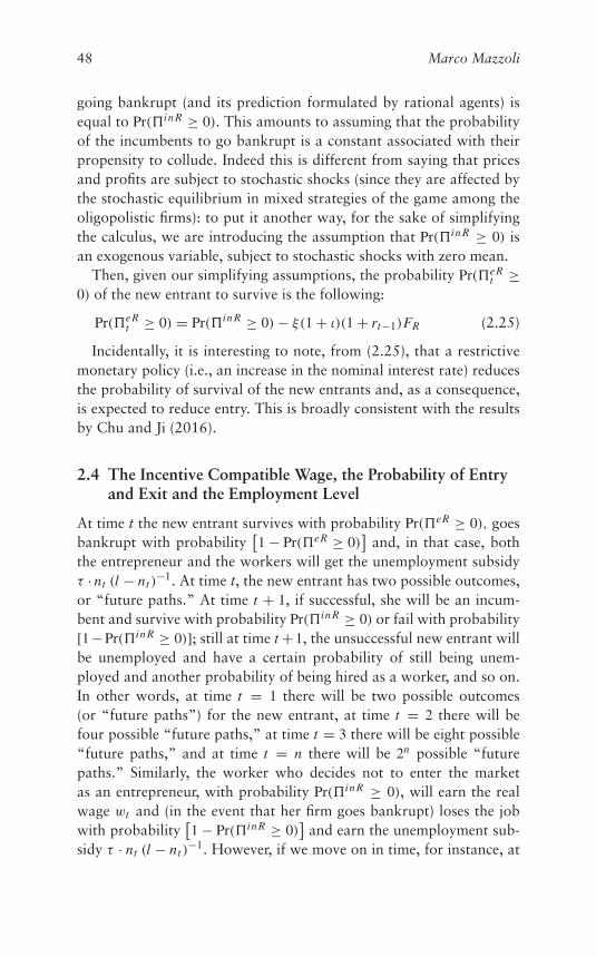
48 Marco Mazzoli
going bankrupt (and its prediction formulated by rational agents) isequal to Pr(�in R ≥ 0). This amounts to assuming that the probabilityof the incumbents to go bankrupt is a constant associated with theirpropensity to collude. Indeed this is different from saying that pricesand profits are subject to stochastic shocks (since they are affected bythe stochastic equilibrium in mixed strategies of the game among theoligopolistic firms): to put it another way, for the sake of simplifyingthe calculus, we are introducing the assumption that Pr(�in R ≥ 0) isan exogenous variable, subject to stochastic shocks with zero mean.
Then, given our simplifying assumptions, the probability Pr(�eRt ≥
0) of the new entrant to survive is the following:
Pr(�eRt ≥ 0) = Pr(�in R ≥ 0) − ξ(1 + ι)(1 + rt−1)FR (2.25)
Incidentally, it is interesting to note, from (2.25), that a restrictivemonetary policy (i.e., an increase in the nominal interest rate) reducesthe probability of survival of the new entrants and, as a consequence,is expected to reduce entry. This is broadly consistent with the resultsby Chu and Ji (2016).
2.4 The Incentive Compatible Wage, the Probability of Entryand Exit and the Employment Level
At time t the new entrant survives with probability Pr(�eR ≥ 0), goesbankrupt with probability
[1 − Pr(�eR ≥ 0)
]and, in that case, both
the entrepreneur and the workers will get the unemployment subsidyτ · nt (l − nt )
−1. At time t, the new entrant has two possible outcomes,or “future paths.” At time t + 1, if successful, she will be an incum-bent and survive with probability Pr(�in R ≥ 0) or fail with probability[1−Pr(�in R ≥ 0)]; still at time t +1, the unsuccessful new entrant willbe unemployed and have a certain probability of still being unem-ployed and another probability of being hired as a worker, and so on.In other words, at time t = 1 there will be two possible outcomes(or “future paths”) for the new entrant, at time t = 2 there will befour possible “future paths,” at time t = 3 there will be eight possible“future paths,” and at time t = n there will be 2n possible “futurepaths.” Similarly, the worker who decides not to enter the marketas an entrepreneur, with probability Pr(�in R ≥ 0), will earn the realwage wt and (in the event that her firm goes bankrupt) loses the jobwith probability
[1 − Pr(�in R ≥ 0)
]and earn the unemployment sub-
sidy τ · nt (l − nt )−1. However, if we move on in time, for instance, at
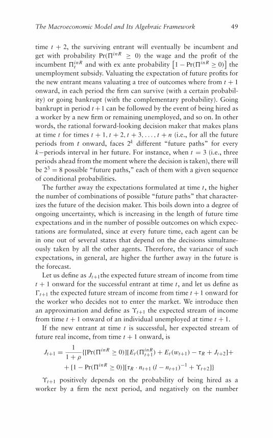
The Macroeconomic Model and Its Algebraic Framework 49
time t + 2, the surviving entrant will eventually be incumbent andget with probability Pr(�in R ≥ 0) the wage and the profit of theincumbent �in R
t and with ex ante probability[1 − Pr(�in R ≥ 0)
]the
unemployment subsidy. Valuating the expectation of future profits forthe new entrant means valuating a tree of outcomes where from t + 1onward, in each period the firm can survive (with a certain probabil-ity) or going bankrupt (with the complementary probability). Goingbankrupt in period t +1 can be followed by the event of being hired asa worker by a new firm or remaining unemployed, and so on. In otherwords, the rational forward-looking decision maker that makes plansat time t for times t + 1, t + 2, t + 3, . . . , t + n (i.e., for all the futureperiods from t onward, faces 2k different “future paths” for everyk−periods interval in her future. For instance, when t = 3 (i.e., threeperiods ahead from the moment where the decision is taken), there willbe 23 = 8 possible “future paths,” each of them with a given sequenceof conditional probabilities.
The further away the expectations formulated at time t , the higherthe number of combinations of possible “future paths” that character-izes the future of the decision maker. This boils down into a degree ofongoing uncertainty, which is increasing in the length of future timeexpectations and in the number of possible outcomes on which expec-tations are formulated, since at every future time, each agent can bein one out of several states that depend on the decisions simultane-ously taken by all the other agents. Therefore, the variance of suchexpectations, in general, are higher the further away in the future isthe forecast.
Let us define as Jt+1the expected future stream of income from timet + 1 onward for the successful entrant at time t , and let us define as�t+1 the expected future stream of income from time t + 1 onward forthe worker who decides not to enter the market. We introduce thenan approximation and define as ϒt+1 the expected stream of incomefrom time t + 1 onward of an individual unemployed at time t + 1.
If the new entrant at time t is successful, her expected stream offuture real income, from time t + 1 onward, is
Jt+1 = 1
1 + ρ{[Pr(�in R ≥ 0)][Et (�
in Rt+1) + Et (wt+1) − τR + Jt+2]+
+ [1 − Pr(�in R ≥ 0)][τR · nt+1 (l − nt+1)−1 + ϒt+2]}
ϒt+1 positively depends on the probability of being hired as aworker by a firm the next period, and negatively on the number
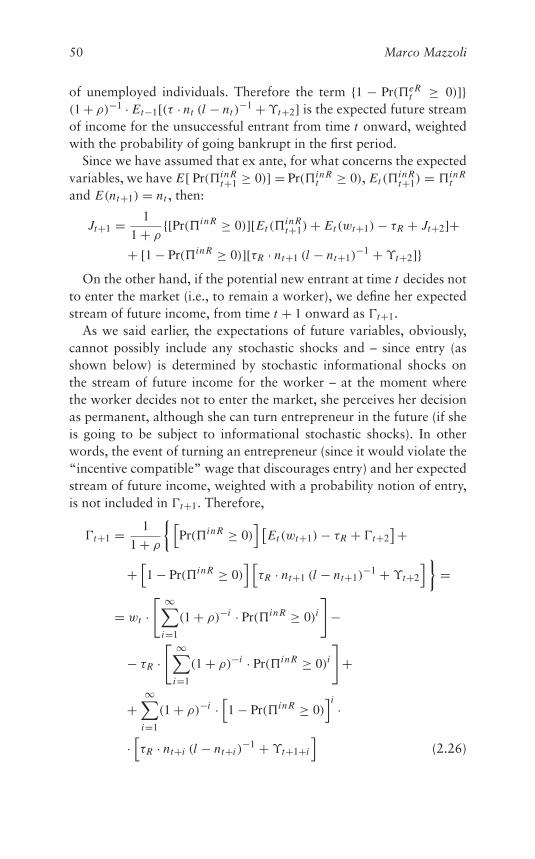
50 Marco Mazzoli
of unemployed individuals. Therefore the term {1 − Pr(�eRt ≥ 0)]}
(1 + ρ)−1 · Et−1[(τ · nt (l − nt )−1 +ϒt+2] is the expected future stream
of income for the unsuccessful entrant from time t onward, weightedwith the probability of going bankrupt in the first period.
Since we have assumed that ex ante, for what concerns the expectedvariables, we have E[ Pr(�in R
t+1 ≥ 0)] = Pr(�in Rt ≥ 0), Et (�
in Rt+1) = �in R
tand E(nt+1) = nt , then:
Jt+1 = 1
1 + ρ{[Pr(�in R ≥ 0)][Et (�
in Rt+1) + Et (wt+1) − τR + Jt+2]+
+ [1 − Pr(�in R ≥ 0)][τR · nt+1 (l − nt+1)−1 + ϒt+2]}
On the other hand, if the potential new entrant at time t decides notto enter the market (i.e., to remain a worker), we define her expectedstream of future income, from time t + 1 onward as �t+1.
As we said earlier, the expectations of future variables, obviously,cannot possibly include any stochastic shocks and – since entry (asshown below) is determined by stochastic informational shocks onthe stream of future income for the worker – at the moment wherethe worker decides not to enter the market, she perceives her decisionas permanent, although she can turn entrepreneur in the future (if sheis going to be subject to informational stochastic shocks). In otherwords, the event of turning an entrepreneur (since it would violate the“incentive compatible” wage that discourages entry) and her expectedstream of future income, weighted with a probability notion of entry,is not included in �t+1. Therefore,
�t+1 = 1
1 + ρ
{ [Pr(�in R ≥ 0)
] [Et (wt+1) − τR + �t+2
]++[1 − Pr(�in R ≥ 0)
] [τR · nt+1 (l − nt+1)
−1 + ϒt+2
] }=
= wt ·[ ∞∑
i=1
(1 + ρ)−i · Pr(�in R ≥ 0)i
]−
− τR ·[ ∞∑
i=1
(1 + ρ)−i · Pr(�in R ≥ 0)i
]+
+∞∑
i=1
(1 + ρ)−i ·[1 − Pr(�in R ≥ 0)
]i ·
·[τR · nt+i (l − nt+i )
−1 + ϒt+1+i
](2.26)
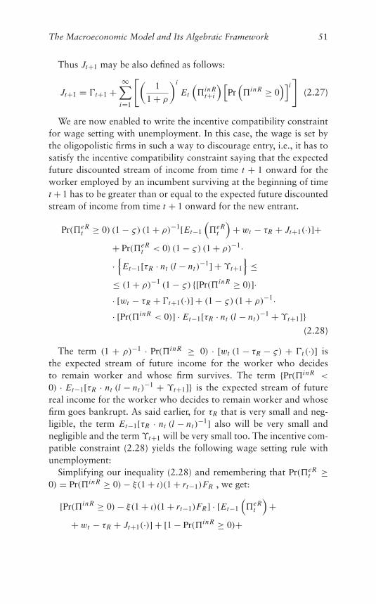
The Macroeconomic Model and Its Algebraic Framework 51
Thus Jt+1 may be also defined as follows:
Jt+1 = �t+1 +∞∑
i=1
[(1
1 + ρ
)i
Et
(�in R
t+i
) [Pr(�in R ≥ 0
)]i]
(2.27)
We are now enabled to write the incentive compatibility constraintfor wage setting with unemployment. In this case, the wage is set bythe oligopolistic firms in such a way to discourage entry, i.e., it has tosatisfy the incentive compatibility constraint saying that the expectedfuture discounted stream of income from time t + 1 onward for theworker employed by an incumbent surviving at the beginning of timet + 1 has to be greater than or equal to the expected future discountedstream of income from time t + 1 onward for the new entrant.
Pr(�eRt ≥ 0) (1 − ς) (1 + ρ)−1[Et−1
(�eR
t
)+ wt − τR + Jt+1(·)]+
+ Pr(�eRt < 0) (1 − ς) (1 + ρ)−1·
·{
Et−1[τR · nt (l − nt )−1] + ϒt+1
}≤
≤ (1 + ρ)−1 (1 − ς) {[Pr(�in R ≥ 0)]·· [wt − τR + �t+1(·)] + (1 − ς) (1 + ρ)−1·· [Pr(�in R < 0)] · Et−1[τR · nt (l − nt )
−1 + ϒt+1]}(2.28)
The term (1 + ρ)−1 · Pr(�in R ≥ 0) · [wt (1 − τR − ς) + �t (·)] isthe expected stream of future income for the worker who decidesto remain worker and whose firm survives. The term {Pr(�in R <
0) · Et−1[τR · nt (l − nt )−1 + ϒt+1]} is the expected stream of future
real income for the worker who decides to remain worker and whosefirm goes bankrupt. As said earlier, for τR that is very small and neg-ligible, the term Et−1[τR · nt (l − nt )
−1] also will be very small andnegligible and the term ϒt+1 will be very small too. The incentive com-patible constraint (2.28) yields the following wage setting rule withunemployment:
Simplifying our inequality (2.28) and remembering that Pr(�eRt ≥
0) = Pr(�in R ≥ 0) − ξ(1 + ι)(1 + rt−1)FR , we get:
[Pr(�in R ≥ 0) − ξ(1 + ι)(1 + rt−1)FR] · [Et−1
(�eR
t
)+
+ wt − τR + Jt+1(·)] + [1 − Pr(�in R ≥ 0)+
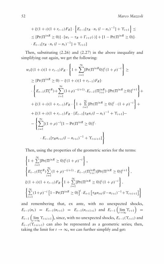
52 Marco Mazzoli
+ ξ(1 + ι)(1 + rt−1)FR] ·{
Et−1[τR · nt (l − nt )−1] + ϒt+1
}≤
≤ [Pr(�in R ≥ 0)] · [wt − τR + �t+1(·)] + [1 − Pr(�in R ≥ 0)]·· Et−1[τR · nt (l − nt )
−1] + ϒt+1]Then, substituting (2.26) and (2.27) in the above inequality and
simplifying out again, we get the following:
wtξ(1 + ι)(1 + rt−1)FR ·{
1 +∞∑
i=1
[Pr(�in R0)]i (1 + ρ)−i
}≥
≥ [Pr(�in R ≥ 0) − ξ(1 + ι)(1 + rt−1)FR]·
·{
Et−1(�eRt )+
∞∑i=1
(1+ρ)−(i+1) ·Et−1(�in Rt+i )·[Pr(�in R ≥0)]i+1
}+
+ ξ(1 + ι)(1 + rt−1)FR ·{
1 + ∞�
i=1[Pr(�in R ≥ 0)]i · (1 + ρ)−i
}+
+ ξ(1 + ι)(1 + rt−1)FR · {Et−1[τRnt (l − nt )−1 + ϒt+1]−
−{ ∞∑
i=1
[(1 + ρ)−i [1 − Pr(�in R ≥ 0)]i ·
· Et−1[τRnt+i (l − nt+i )−1 + ϒt+i+1]
}
Then, using the properties of the geometric series for the terms:{1 +
∞∑i=1
[Pr(�in R ≥ 0)]i (1 + ρ)−i}
,{Et−1(�
eRt )
∞∑i=1
(1 + ρ)−(i+1) · Et−1(�in Rt+i )[Pr(�in R ≥ 0)]i+1
},
ξ(1 + ι)(1 + rt−1)FR
{1 +
∞∑i=1
[Pr(�in R ≥ 0)]i (1 + ρ)−i},{ ∞∑
i=1(1+ρ)−i
[1−Pr(�in R ≥ 0)
]i ·Et−1[τRnt+i (l−nt+i )
−1+ϒt+i+1]}
and remembering that, ex ante, with no unexpected shocks,
Et−1(nt ) = Et−1(nt+1) = Et−1(nt+1+i ) and Et−1
(lim
t→∞ϒt+1
)=
Et−1
(lim
t→∞ϒt+i+1
), since, with no unexpected shocks, Et−1(ϒt+1) and
Et−1(ϒt+i+1) can also be represented as a geometric series; then,taking the limit for t → ∞, we can further simplify and get:
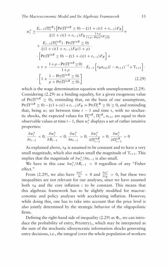
The Macroeconomic Model and Its Algebraic Framework 53
w∗t ≥ Et−1(�
eRt )
[Pr(�in R ≥ 0) − ξ(1 + ι)(1 + rt−1)FR
]ξ(1 + ι)(1 + rt−1)FR
1+ρ
1+ρ−Pr(π in R≥0)
+
+ Et−1(�in Rt ) · Pr(�in R ≥ 0)
ξ(1 + ι)(1 + rt−1)FR(1 + ρ)·
·[Pr(�in R ≥ 0) − ξ(1 + ι)(1 + rt−1)FR
]+
+ τ + 1+ρ−Pr(�in R ≥0)
1+ρ· Et−1
[τRnt+1(l − nt+1)
−1+ϒt+1
]·
·[
1 + 1 − Pr(�in R ≥ 0)
ρ + Pr(�in R ≥ 0)
](2.29)
which is the wage determination equation with unemployment (2.29).Considering (2.29) as a binding equality, for a given exogenous valueof Pr(�in R ≥ 0), reminding that, on the basis of our assumptions,Pr(�in R ≥ 0)−ξ(1+ ι)(1+rt−1)FR = Pr(�eR
t ≥ 0) ≥ 0, and remindingthat, being wt set between time t − 1 and time t , with no stochas-tic shocks, the expected values for �in R
t , �eRt , nt+i are equal to their
observable values at time t−1, then w∗t displays a set of rather intuitive
properties:
∂w∗t
∂rt−1< 0; ∂w∗
t
∂Rt−1< 0; ∂w∗
t
∂nt−1> 0; ∂w∗
t
∂�in Rt−1
> 0; ∂w∗t
∂�eRt−1
> 0
As explained above, τR is assumed to be constant and to have a verysmall magnitude, which also makes small the magnitude of ϒt+1. Thisimplies that the magnitude of ∂w∗
t /∂nt−1 is also small.We have in this case ∂w∗
t /∂Rt−1 < 0 regardless of any “Fishereffect.”
From (2.29), we also have ∂w∗t
∂ι< 0 and ∂w∗
t∂τR
> 0, but these twoinequalities are not relevant for our analyses, since we have assumedboth τR and the core inflation ι to be constant. This means thatthis algebraic framework has to be slightly modified for macroe-conomic and policy analyses with accelerating inflation. However,while doing this, one has to take into account that the price level isalso jointly determined by the strategic behavior of the oligopolisticfirms.
Defining the right-hand side of inequality (2.29) as t , we can intro-duce the probability of entry, Pr(entry)t , which may be interpreted asthe sum of the stochastic idiosyncratic information shocks generatingentry decisions, i.e., the integral (over the whole population of workers
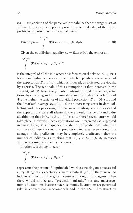
54 Marco Mazzoli
nt (1 − ht ) at time t of the perceived probability that the wage is set ata lower level than the expected present discounted value of the futureprofits as an entrepreneur in case of entry.
Pr(entry)t =nt (1−ht )∫
0
(Pr(wt < Et−1,i (t ))i di (2.30)
Given the equilibrium equality wt = Et−1,i (t ), the expression
nt (1−ht )∫0
(Pr(wt < Et−1,i (t ))i di
is the integral of all the idiosyncratic information shocks on Et−1,i (t )
for any individual worker i at time t , which depends on the variance ofthe expectation Et−1,i (t ), which is induced, as indicated previously,by var(�t ). The rationale of this assumption is that increases in thevolatility of �t force the potential entrants to update their expecta-tions, by collecting and processing data and the higher the volatility of�t , the higher the variance of individual predictions Et−1,i (t ) aroundthe “market” average Et−1(t ), due to increasing costs in data col-lecting and data processing. If there were no idiosyncratic shocks andthe expectations were all identical, there would not be any individu-als thinking that Pr(wt < Et−1,i (t ))i and, therefore, no entry wouldtake place. However, since expectations are interpreted (as suggestedin Lucas 1976) as a frequency distribution of predictions, when thevariance of these idiosyncratic predictions increase (even though theaverage of the predictions may be completely unaffected), then thenumber of individuals i thinking that Pr(wt < Et−1,i (t ))i increasesand, as a consequence, entry increases.
In other words, the integral
nt (1−ht )∫0
(Pr(wt < Et−1,i (t ))i di
represents the portion of “optimistic” workers trusting on a successfulentry. If agents’ expectations were identical (i.e., if there were nohidden actions nor diverging incentives among all the agents), thenthere would not be any “prediction mistake” nor any macroeco-nomic fluctuations, because macroeconomic fluctuations are generated(like in conventional macromodels and in the DSGE literature) by
The Macroeconomic Model and Its Algebraic Framework 55
stochastic shocks: we have here shocks generated by the outcomeamong oligopolistic firms, and not the technology shocks that gen-erate the business cycle in the Real Business Cycle literature andin most DSGE contributions; however, without these shocks, expec-tations would turn out to be “true” ex post. Nevertheless, sinceexpectations are not a point value and the stochastic shocks gener-ate macroeconomic fluctuations, the rational agents, time after time,have to adjust their expectations to the observable variables, thatinclude the outcomes of the stochastic shocks. Like in conventionalmacromodels, these shocks generate the divergence between predictedand ex post observable variables. This is the reason why in thismodel it is assumed that the expectation of each relevant variableis equal to its last observable value. Of course, the market expec-tation is interpreted as the average of the expectations of all theindividuals.
2.5 A Digression on the Link Between the Labor MarketEquilibrium, the Firm’s Output and the Entry Decision
This work follows, in spirit (although not in some details of themodeling technique and in some algebraic features), Aoki andYoshikawa’s (2007) approach to macroeconomic modeling. Looselyspeaking, there is a correspondence between the assumptions by Aokiand Yoshikawa (2007, ch. 2) and our assumption on how the inter-acting agents behave at a microeconomic level. Aoki and Yoshikawa(2007) assume that agents have binary choices. The two choices canbe represented by two states (say state 0 and state 1). If we have nagents, the state of n agents may be represented as s = (s1, s2, . . . , sn),where the choice by agent i is denoted by si = 1 or si = 0 and so on. Aset of all the possible values of s is called “state space” S. The purposeof this assumption is to describe the dynamic process of how do agentsrevise their choices in time, due to incentives, externalities, costs, andunexpected news. Since we are interested in the time evolution of thestates, we consider a stochastic process in discrete time (differentlyfrom Aoki and Yoshikawa, who consider jump Markov processes incontinuous time). However, in our formalization of the jump Markovprocess, we use more variables than Aoki and Yoshikawa to introduceour formalization. We start by following the notation by Aoki andYoshikawa, in terms of transition rates, between time t − 1 and t :
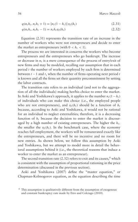
56 Marco Mazzoli
q(nt ht , nt ht + 1) = [nt (1 − ht )] η1(ht ) (2.31)
q(nt ht , nt ht − 1) = nt htη2(ht ) (2.32)
Equation (2.31) represents the transition rate of an increase in thenumber of workers who were not entrepreneurs and decide to enterthe market as entrepreneurs (with 0 < ht < 1).
The process we are interested in concerns the workers who becomeentrepreneurs and the entrepreneurs who go bankrupt. The increaseor decrease in nt is a mere consequence of the process of entry/exit ofnew firms and may be modeled, recalling our assumption that in eachperiod t the number of workers employed by each firm is determinedbetween t −1 and t , when the number of firms operating next period tis known and all the firms set their quantity precommitment by settingthe labor contracts.
The transition rate refers to an individual (and not to the aggrega-tion of all the individuals) making her/his choice to enter the market.In Aoki and Yoshikawa’s approach, it applies to the number nt (1−ht )
of individuals who can make this choice (i.e., the employed peoplewho are not entrepreneurs), and η1(ht ) should be a function of ht
because, according to Aoki and Yoshikawa, it would not be rationalfor an individual to neglect externalities; therefore, it is a decreasingfunction of ht because the decision to enter the market is discour-aged by a high number of existing entrepreneurs. The higher the ht ,
the smaller the η1(ht ). In the benchmark case, where the economyreaches full employment, the workers will be remunerated exactly likethe entrepreneurs, and there will be no incentive and no room fornew entries. As shown below, we follow this assumption by Aokiand Yoshikawa, but we attempt to model more in detail the behav-ioral assumptions behind it (i.e., the theoretical reasons that induce aworker to enter the market as an entrepreneur).
The second transition rate (2.32) refers to exit and its causes,4 whichis consistent with the assumption of proportional rationing in the pricedetermination (discussed in the previous section).
Aoki and Yoshikawa (2007) define the “master equation,” orChapman-Kolmogorov equation, as the equation describing the time
4 This assumption is qualitatively different from the assumption of exogenousand constant bankruptcy rate made by Etro and Colciago (2010).
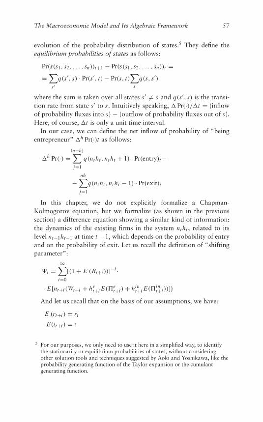
The Macroeconomic Model and Its Algebraic Framework 57
evolution of the probability distribution of states.5 They define theequilibrium probabilities of states as follows:
Pr(s(s1, s2, . . . , sn))t+1 − Pr(s(s1, s2, . . . , sn))t ==∑
s′q(s′, s) · Pr(s′, t) − Pr(s, t)
∑s
q(s, s′)
where the sum is taken over all states s′ �= s and q(s′, s) is the transi-tion rate from state s′ to s. Intuitively speaking, �Pr(·)/�t = (inflowof probability fluxes into s) − (outflow of probability fluxes out of s).Here, of course, �t is only a unit time interval.
In our case, we can define the net inflow of probability of “beingentrepreneur” �h Pr(·)t as follows:
�h Pr(·) =(n−h)∑
j=1
q(nt ht , nt ht + 1) · Pr(entry)t−
−nh∑j=1
q(nt ht , nt ht − 1) · Pr(exit)t
In this chapter, we do not explicitly formalize a Chapman-Kolmogorov equation, but we formalize (as shown in the previoussection) a difference equation showing a similar kind of information:the dynamics of the existing firms in the system nt ht , related to itslevel nt−1ht−1 at time t − 1, which depends on the probability of entryand on the probability of exit. Let us recall the definition of “shiftingparameter”:
�t =∞∑
i=0
[(1 + E (Rt+i ))]−i ·
· E[nt+i (Wt+i + het+i E(�e
t+i ) + hint+i E(�in
t+i ))]}And let us recall that on the basis of our assumptions, we have:
E (rt+i ) = rt
E(ιt+i ) = ι
5 For our purposes, we only need to use it here in a simplified way, to identifythe stationarity or equilibrium probabilities of states, without consideringother solution tools and techniques suggested by Aoki and Yoshikawa, like theprobability generating function of the Taylor expansion or the cumulantgenerating function.
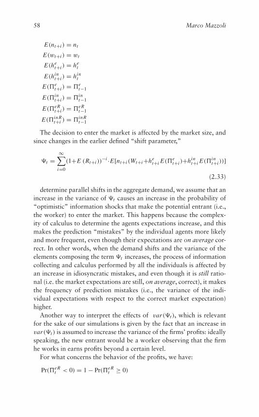
58 Marco Mazzoli
E(nt+i ) = nt
E(wt+i ) = wt
E(het+i ) = he
t
E(hint+i ) = hin
t
E(�et+i ) = �e
t−1
E(�int+i ) = �in
t−1
E(�eRt+i ) = �eR
t−1
E(�in Rt+i ) = �in R
t−1
The decision to enter the market is affected by the market size, andsince changes in the earlier defined “shift parameter,”
�t =∞∑
i=0
(1+E (Rt+i ))−i ·E[nt+i (Wt+i+he
t+i E(�et+i )+hin
t+i E(�int+i ))]
(2.33)
determine parallel shifts in the aggregate demand, we assume that anincrease in the variance of �t causes an increase in the probability of“optimistic” information shocks that make the potential entrant (i.e.,the worker) to enter the market. This happens because the complex-ity of calculus to determine the agents expectations increase, and thismakes the prediction “mistakes” by the individual agents more likelyand more frequent, even though their expectations are on average cor-rect. In other words, when the demand shifts and the variance of theelements composing the term �t increases, the process of informationcollecting and calculus performed by all the individuals is affected byan increase in idiosyncratic mistakes, and even though it is still ratio-nal (i.e. the market expectations are still, on average, correct), it makesthe frequency of prediction mistakes (i.e., the variance of the indi-vidual expectations with respect to the correct market expectation)higher.
Another way to interpret the effects of var(�t ), which is relevantfor the sake of our simulations is given by the fact that an increase invar(�t ) is assumed to increase the variance of the firms’ profits: ideallyspeaking, the new entrant would be a worker observing that the firmhe works in earns profits beyond a certain level.
For what concerns the behavior of the profits, we have:
Pr(�eRt < 0) = 1 − Pr(�eR
t ≥ 0)
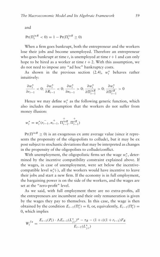
The Macroeconomic Model and Its Algebraic Framework 59
and
Pr(�in Rt < 0) = 1 − Pr(�in R
t ≥ 0)
When a firm goes bankrupt, both the entrepreneur and the workerslose their jobs and become unemployed. Therefore an entrepreneurwho goes bankrupt at time t , is unemployed at time t +1 and can onlyhope to be hired as a worker at time t + 2. With this assumption, wedo not need to impose any “ad hoc” bankruptcy costs.
As shown in the previous section (2.4), w∗t behaves rather
intuitively:
∂w∗t
∂rt−1< 0; ∂w∗
t
∂Rt−1< 0; ∂w∗
t
∂nt−1> 0; ∂w∗
t
∂�in Rt−1
> 0; ∂w∗t
∂�eRt−1
> 0
Hence we may define w∗t as the following generic function, which
also includes the assumption that the workers do not suffer frommoney illusion:
w∗t = w∗
t (−
rt−1,+
nt−1,
+�in R
t−1,
+�eR
t−1)
Pr(�in R ≥ 0) is an exogenous ex ante average value (since it repre-sents the propensity of the oligopolists to collude), but it may be expost subject to stochastic deviations that may be interpreted as changesin the propensity of the oligopolists to collude/conflict.
With unemployment, the oligopolistic firms set the wage w∗t , deter-
mined by the incentive compatibility constraint explained above. Ifthe wages, in case of unemployment, were set below the incentive-compatible level w∗
t (·), all the workers would have incentive to leavetheir jobs and start a new firm. If the economy is in full employment,the bargaining power is on the side of the workers, and the wages areset at the “zero-profit” level.
As we said, with full employment there are no extra-profits, allthe entrepreneurs are incumbent and their only remuneration is givenby the wages they pay to themselves. In this case, the wage is thenobtained by the condition Et−1(�
et ) = 0, or, equivalently, Et−1(�
et ) =
0, which implies
W f ut = Et−1(Pt ) · �Et−1(L∗
j,t )α − τR − (1 + ι)(1 + rt−1)FR
Et−1(L∗j,t )
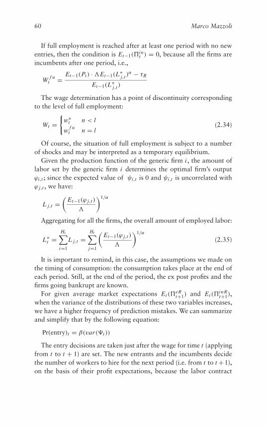
60 Marco Mazzoli
If full employment is reached after at least one period with no newentries, then the condition is Et−1(�
int ) = 0, because all the firms are
incumbents after one period, i.e.,
W f ut = Et−1(Pt ) · �Et−1(L∗
j,t )α − τR
Et−1(L∗j,t )
The wage determination has a point of discontinuity correspondingto the level of full employment:
Wt ={w∗
t n < l
wf u
t n = l(2.34)
Of course, the situation of full employment is subject to a numberof shocks and may be interpreted as a temporary equilibrium.
Given the production function of the generic firm i , the amount oflabor set by the generic firm i determines the optimal firm’s outputϕi,t ; since the expected value of ψi,t is 0 and ψi,t is uncorrelated withϕ j,t , we have:
L j,t =(
Et−1(ϕ j,t )
�
)1/α
Aggregating for all the firms, the overall amount of employed labor:
L∗t =
Ht∑i=1
L j,t =Ht∑
j=1
(Et−1(ϕ j,t )
�
)1/α
(2.35)
It is important to remind, in this case, the assumptions we made onthe timing of consumption: the consumption takes place at the end ofeach period. Still, at the end of the period, the ex post profits and thefirms going bankrupt are known.
For given average market expectations Et (�eRt+1) and Et (�
in Rt+1),
when the variance of the distributions of these two variables increases,we have a higher frequency of prediction mistakes. We can summarizeand simplify that by the following equation:
Pr(entry)t = β(var(�t ))
The entry decisions are taken just after the wage for time t (applyingfrom t to t + 1) are set. The new entrants and the incumbents decidethe number of workers to hire for the next period (i.e. from t to t + 1),on the basis of their profit expectations, because the labor contract
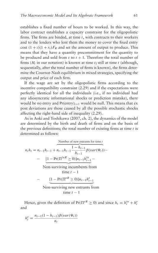
The Macroeconomic Model and Its Algebraic Framework 61
establishes a fixed number of hours to be worked. In this way, thelabor contract establishes a capacity constraint for the oligopolisticfirms. The firms are binded, at time t , with contracts to their workersand to the lenders who lent them the money to cover the fixed entrycost (1 + ι)(1 + rt )FR and set the amount of output to produce. Thismeans that they have a quantity precommitment for the quantity tobe produced and sold from t to t + 1. Therefore the total number offirms (Ht in our notation) is known at time t ; still at time t (although,sequentially, after the total number of firms is known), the firms deter-mine the Cournot-Nash equilibrium in mixed strategies, specifying theoutput and price of each firm.
If the wage are set by the oligopolistic firms according to theincentive compatibility constraint (2.29) and if the expectations wereperfectly identical for all the individuals (i.e., if no individual hadany idiosyncratic informational shocks or prediction mistake), therewould be no entry and Pr(entry)t+1 would be null. This means that expost deviations are those caused by all the possible stochastic shocksaffecting the right-hand side of inequality (2.29).
As in Aoki and Yoshikawa (2007, ch. 2), the dynamics of the modelare determined by the birth and death of firms and on the basis ofthe previous definitions; the total number of existing firms at time t isdetermined as follows:
nt ht = nt−1ht−1 +Number of new entrants for time t︷ ︸︸ ︷
nt−1ht−11 − ht−1
ht−1β(var(�t ))−
− [1 − Pr(�in R ≥ 0)]nt−1hint−1︸ ︷︷ ︸−
Non-surviving incumbents fromtime t − 1
− [1 − Pr(�eR ≥ 0)]nt−1het−1︸ ︷︷ ︸
Non-surviving new entrants fromtime t − 1
Hence, given the definition of Pr(�eR ≥ 0) and since ht = hint + he
tand
het = nt−1(1 − ht−1)β(var(�t ))
nt
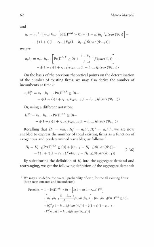
62 Marco Mazzoli
and
ht = n−1t · {nt−1ht−1
[Pr(�in R ≥ 0) + (1 − ht )h
−1t β(var(�t ))
]−
− ξ(1 + ι)(1 − rt−1)FR(1 − ht−2)β(var(�t−1))}we get:
nt ht = nt−1ht−1
[Pr(�in R ≥ 0) + 1 − ht−1
ht−1β(var(�t ))
]−
− ξ(1 + ι)(1 + rt−1)FRnt−2(1 − ht−2)β(var(�t−1))
On the basis of the previous theoretical points on the determinationof the number of existing firms, we may also derive the number ofincumbents at time t :
nt hint = nt−1ht−1 · Pr(�in R ≥ 0)−
− ξ(1 + ι)(1 + rt−2)FRnt−2(1 − ht−2)β(var(�t−1))
Or, using a different notation:
Hint = nt−1ht−1 · Pr(�in R ≥ 0)−
− ξ(1 + ι)(1 + rt−2)FRnt−2(1 − ht−2)β(var(�t−1))
Recalling that Ht = nt ht , Het = nt he
t , Hint = nt hin
t , we are nowenabled to express the number of total existing firms as a function ofexogenous and predetermined variables, as follows:6
Ht = Ht−1[Pr(�in R ≥ 0)] + [(nt−1 − Ht−1)β(var(�t )]−− ξ(1 + ι)(1 + rt−1)FR(nt−2 − Ht−2)β(var(�t−1))
(2.36)
By substituting the definition of Ht into the aggregate demand andrearranging, we get the following definition of the aggregate demand:
6 We may also define the overall probability of exit, for the all existing firms(both new entrants and incumbents):
Pr(exit)t = 1 − Pr(�in R ≥ 0) +[ξ(1 + ι)(1 + rt−1)F R
]·[
nt−1ht−1(1 − ht−1)
ht−1β(var(�t ))
]· {nt−1ht−1[Pr(�in R ≥ 0) ·
+ h−1t−1(1 − ht−1)β(var(�t ))] − ξ(1 + ι)(1 + rt−1) ·
· F Rnt−2(1 − ht−2)β(var(�t−1))}
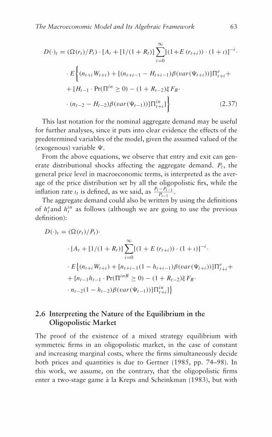
The Macroeconomic Model and Its Algebraic Framework 63
D(·)t = (�(rt )/Pt ) · [At + [1/(1 + Rt )]∞∑
i=0
[(1+E (rt+i )) · (1 + ι)]−i ·
· E
{(nt+i Wt+i ) + [(nt+i−1 − Ht+i−1)β(var(�t+i ))]�e
t+i++ [Ht−1 · Pr(�in ≥ 0) − (1 + Rt−2)ξFR ·· (nt−2 − Ht−2)β(var(�t−1))]�in
t+i ]}
(2.37)
This last notation for the nominal aggregate demand may be usefulfor further analyses, since it puts into clear evidence the effects of thepredetermined variables of the model, given the assumed valued of the(exogenous) variable �.
From the above equations, we observe that entry and exit can gen-erate distributional shocks affecting the aggregate demand. Pt , thegeneral price level in macroeconomic terms, is interpreted as the aver-age of the price distribution set by all the oligopolistic firs, while theinflation rate ιt is defined, as we said, as Pt −Pt−1
Pt−1.
The aggregate demand could also be written by using the definitionsof he
t and hint as follows (although we are going to use the previous
definition):
D(·)t = (�(rt )/Pt )·
· [At + [1/(1 + Rt )]∞∑
i=0
[(1 + E (rt+i )) · (1 + ι)]−i ·
· E{(nt+i Wt+i ) + [nt+i−1(1 − ht+i−1)β(var(�t+i ))]�e
t+i++ [nt−1ht−1 · Pr(�in R ≥ 0) − (1 + Rt−2)ξFR ·· nt−2(1 − ht−2)β(var(�t−1))]�in
t+i ]}
2.6 Interpreting the Nature of the Equilibrium in theOligopolistic Market
The proof of the existence of a mixed strategy equilibrium withsymmetric firms in an oligopolistic market, in the case of constantand increasing marginal costs, where the firms simultaneously decideboth prices and quantities is due to Gertner (1985, pp. 74–98). Inthis work, we assume, on the contrary, that the oligopolistic firmsenter a two-stage game à la Kreps and Scheinkman (1983), but with
64 Marco Mazzoli
the modifications and extensions provided by Madden (1998), asexplained in this section.
Dasgupta and Maskin (1986) proved the general existence of mixedstrategy equilibrium in a Bertrand-Edgeworth model with a continu-ous demand function that is equal to zero for sufficiently high pricesand with discontinuities in the payoffs of the oligopolistic firms. Allenand Hellwig (1986) extended the result to the case of a demand curvethat does not intersect the horizontal axis, and Maskin (1986) provedthe existence result of a mixed strategy equilibrium in an oligopolisticmodel where firms simultaneously choose both prices and quantitiesto a case where firms’ symmetry is not required and with rather gen-eral costs functions. Maskin’s provides his proofs for a duopolisticmarket, but he points out that they are valid for a finite number ofoligopolistic firms (Maskin, 1986, p. 382). As Vives (2001) points out,the use of mixed strategy equilibria in economic modeling is somehowcontroversial, since “in a mixed-strategy equilibrium all actions in thesupport of the equilibrium distribution of a player are best responsesto the distributions used by the rivals” (Vives, 2001, p. 45). However,Vives suggests that players choices may depend on random factors thatare not relevant for the payoffs and, as Harsanyi (1973) also suggests,an interpretation of mixed strategies as pure strategies in a perturbedgame: in other words, in a mixed-strategy equilibrium, each playermay be using a pure strategy subject to a small random disturbance onhis own payoff. This might happen, for instance, if a firm is observingthe costs of its rival with a slight uncertainty.
This model is broadly consistent with the interpretation byHarsanyi, since it is assumed that the oligopolistic firms imper-fectly observe the cost choices of their rivals and approximate themon the basis of conjectures: in other words, they play a perturbedgame.
The mixed-strategy equilibria are interpreted as stochastic steadystates by (Osborne and Rubinstein, 1994, p. 39), where each occur-rence of the game takes place after n players are randomly chosenfrom different populations. This last interpretation is also consistentwith the assumptions of this model because here the firms inter-acting in the market, due to entry and exit, are not the same ineach occurrence of the game and since entry and exit are affectedby stochastic shocks, the firms existing in each time t are chosenstochastically.
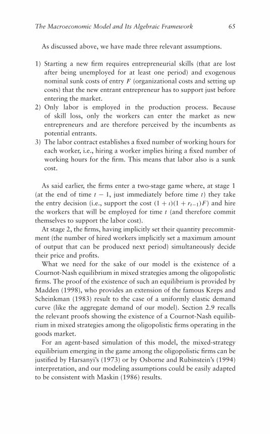
The Macroeconomic Model and Its Algebraic Framework 65
As discussed above, we have made three relevant assumptions.
1) Starting a new firm requires entrepreneurial skills (that are lostafter being unemployed for at least one period) and exogenousnominal sunk costs of entry F (organizational costs and setting upcosts) that the new entrant entrepreneur has to support just beforeentering the market.
2) Only labor is employed in the production process. Becauseof skill loss, only the workers can enter the market as newentrepreneurs and are therefore perceived by the incumbents aspotential entrants.
3) The labor contract establishes a fixed number of working hours foreach worker, i.e., hiring a worker implies hiring a fixed number ofworking hours for the firm. This means that labor also is a sunkcost.
As said earlier, the firms enter a two-stage game where, at stage 1(at the end of time t − 1, just immediately before time t) they takethe entry decision (i.e., support the cost (1 + ι)(1 + rt−1)F) and hirethe workers that will be employed for time t (and therefore committhemselves to support the labor cost).
At stage 2, the firms, having implicitly set their quantity precommit-ment (the number of hired workers implicitly set a maximum amountof output that can be produced next period) simultaneously decidetheir price and profits.
What we need for the sake of our model is the existence of aCournot-Nash equilibrium in mixed strategies among the oligopolisticfirms. The proof of the existence of such an equilibrium is provided byMadden (1998), who provides an extension of the famous Kreps andScheinkman (1983) result to the case of a uniformly elastic demandcurve (like the aggregate demand of our model). Section 2.9 recallsthe relevant proofs showing the existence of a Cournot-Nash equilib-rium in mixed strategies among the oligopolistic firms operating in thegoods market.
For an agent-based simulation of this model, the mixed-strategyequilibrium emerging in the game among the oligopolistic firms can bejustified by Harsanyi’s (1973) or by Osborne and Rubinstein’s (1994)interpretation, and our modeling assumptions could be easily adaptedto be consistent with Maskin (1986) results.
66 Marco Mazzoli
We assume that proportional rationing applies and that the profit(payoff) function of the firm is continuous in prices. We also assumethat the amount of work hired by each firm constitutes a capacityconstraint, on the basis of the labor contracts set for time t , untiltime t + 1.
We want to explicitly formalize another potential source of stochas-tic shocks: conflict. For this purpose, we assume that the quantitiesdecided by the firms, instead of being commodities, are “contracts,”i.e., “commitments” to sell commodities to the customers. These com-mitments are subject to stochastic shocks. These stochastic shocksmay cause some firms to go bankrupt and, in this way, the firms’failure does not imply any lack of rationality in the determina-tion of the Nash Equilibrium among oligopolistic firms becausein the Nash equilibrium in mixed strategies emerging among theoligopolistic firms, the firms’ bankruptcies are not the effects ofa planned choice, but are stochastic. This point also carries rel-evant implications for the determination of the macroeconomicequilibrium.
Given the timing assumptions of this model, both entry costs andlabor costs are sunk for the new entrants. Still, for the timing assump-tions of the model, all the incomes (profits, labor and unemploymentsubsidies) for time t are received at the end of time t: labor costs areaccounted as debt of the firms toward the workers, at the beginning oftime t (and this is why they are sunk), even though they are paid outto workers at the end of time t.
The amount of labor Li,t hired by the generic firm i at time t isdecided on the basis of ex ante expectations. Let us define it as theoptimal ex ante amount of labor, associated with the optimal ex anteindividual firm output Et−1(ϕi,t ) at time t . All the firms, both incum-bents and new entrants, have the same technology and productionfunction. Ex ante expectations, ex ante amount of employed laborand ex ante individual firm’s output, are all chosen on the basis of theex ante demand curve at time t , which is the ex post demand for timet − 1, i.e., the empirically observable demand curve that has emergedafter all the stochastic shocks of the model. All the firms make theirchoices on the basis of the equation of the aggregate demand (i.e., eachfirm picks up a point on the aggregate demand), and the price level isto be interpreted has the ex post weighted average of the differentprices set by the various firms.
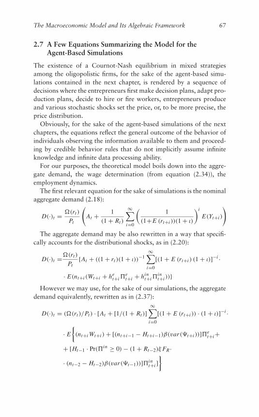
The Macroeconomic Model and Its Algebraic Framework 67
2.7 A Few Equations Summarizing the Model for theAgent-Based Simulations
The existence of a Cournot-Nash equilibrium in mixed strategiesamong the oligopolistic firms, for the sake of the agent-based simu-lations contained in the next chapter, is rendered by a sequence ofdecisions where the entrepreneurs first make decision plans, adapt pro-duction plans, decide to hire or fire workers, entrepreneurs produceand various stochastic shocks set the price, or, to be more precise, theprice distribution.
Obviously, for the sake of the agent-based simulations of the nextchapters, the equations reflect the general outcome of the behavior ofindividuals observing the information available to them and proceed-ing by credible behavior rules that do not implicitly assume infiniteknowledge and infinite data processing ability.
For our purposes, the theoretical model boils down into the aggre-gate demand, the wage determination (from equation (2.34)), theemployment dynamics.
The first relevant equation for the sake of simulations is the nominalaggregate demand (2.18):
D(·)t = �(rt )
Pt
(At + 1
(1 + Rt )
∞∑i=0
(1
(1+E (rt+i ))(1 + ι)
)i
E(Yt+i )
)The aggregate demand may be also rewritten in a way that specifi-
cally accounts for the distributional shocks, as in (2.20):
D(·)t =�(rt )
Pt{At + ((1 + rt )(1 + ι))−1
∞∑i=0
[(1 + E (rt+i ) (1 + ι)]−i ·
· E(nt+i (Wt+i + het+i�
et+i + hin
t+i�int+i ))}
However we may use, for the sake of our simulations, the aggregatedemand equivalently, rewritten as in (2.37):
D(·)t = (�(rt )/Pt ) · [At + [1/(1 + Rt )]∞∑
i=0
[(1 + E (rt+i )) · (1 + ι)]−i ·
· E
{(nt+i Wt+i ) + [(nt+i−1 − Ht+i−1)β(var(�t+i ))]�e
t+i++ [Ht−1 · Pr(�in ≥ 0) − (1 + Rt−2)ξFR ·· (nt−2 − Ht−2)β(var(�t−1))]�in
t+i ]}
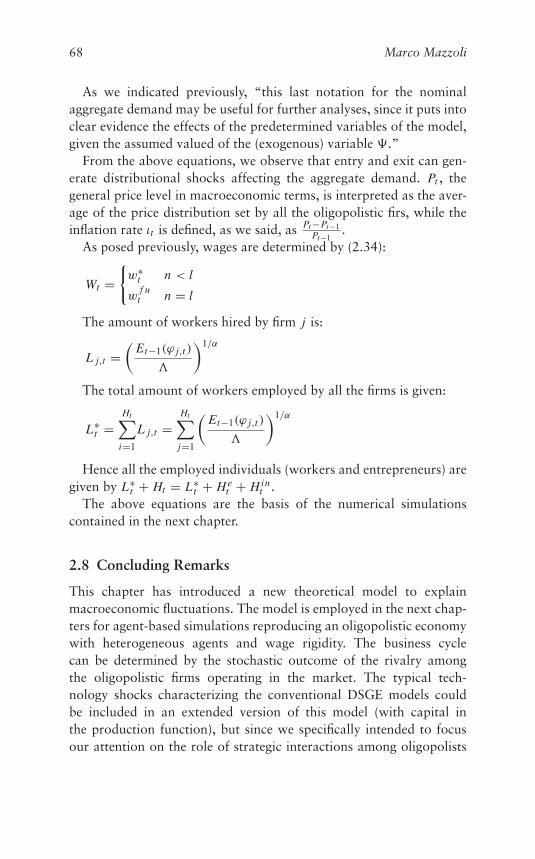
68 Marco Mazzoli
As we indicated previously, “this last notation for the nominalaggregate demand may be useful for further analyses, since it puts intoclear evidence the effects of the predetermined variables of the model,given the assumed valued of the (exogenous) variable �.”
From the above equations, we observe that entry and exit can gen-erate distributional shocks affecting the aggregate demand. Pt , thegeneral price level in macroeconomic terms, is interpreted as the aver-age of the price distribution set by all the oligopolistic firs, while theinflation rate ιt is defined, as we said, as Pt −Pt−1
Pt−1.
As posed previously, wages are determined by (2.34):
Wt ={w∗
t n < l
wf u
t n = l
The amount of workers hired by firm j is:
L j,t =(
Et−1(ϕ j,t )
�
)1/α
The total amount of workers employed by all the firms is given:
L∗t =
Ht∑i=1
L j,t =Ht∑
j=1
(Et−1(ϕ j,t )
�
)1/α
Hence all the employed individuals (workers and entrepreneurs) aregiven by L∗
t + Ht = L∗t + He
t + Hint .
The above equations are the basis of the numerical simulationscontained in the next chapter.
2.8 Concluding Remarks
This chapter has introduced a new theoretical model to explainmacroeconomic fluctuations. The model is employed in the next chap-ters for agent-based simulations reproducing an oligopolistic economywith heterogeneous agents and wage rigidity. The business cyclecan be determined by the stochastic outcome of the rivalry amongthe oligopolistic firms operating in the market. The typical tech-nology shocks characterizing the conventional DSGE models couldbe included in an extended version of this model (with capital inthe production function), but since we specifically intended to focusour attention on the role of strategic interactions among oligopolists
The Macroeconomic Model and Its Algebraic Framework 69
as a potential source of fluctuations, we have chosen, for our pur-pose, to stick to the simplified version of the model presented in thischapter.
A particular feature of our model is the fact that the processof entry/exit potentially interacts with distributional shocks amongworkers and entrepreneurs and (as shown in the next chapters, ded-icated to numerical simulations) with the cyclical or countercyclicalbehavior of firms’ markups.
Our microfoundation allows us to model agents who are heteroge-neous in their budget constraint and have the same preferences andmay change their social group in each period according to a stochas-tic process, interacting both with labor market and with the processof entry/exit. As shown in the next chapters, this modeling strategyallows us to reproduce macroeconomic fluctuations and formalizeother kinds of shocks, like the “conflict” shocks among workers andentrepreneurs.
In this model, the price level (i.e., the average value of the pricedistribution determined by all the oligopolistic firms) is jointly deter-mined by the behavior of the oligopolistic firms and by the monetaryauthorities whose decisions in terms of current and future expectedinterest rates affect the “shift parameter” �t in the aggregate demand.
This means that the effectiveness (or noneffectiveness) of mone-tary policy may also depend on how the decisions of the monetaryauthorities may affect the entry decisions of new potential firms (i.e.,making “overoptimistic” a subset of workers who decide to turn intoentrepreneurs). Also, the price rigidity/flexibility does not only dependon the workers’ market power (like in conventional models) but alsoon the probability of the oligopolistic firms to collude or to chooseprice competition. This last point, as well as the entry decision ofnew firms is modeled here by stochastic variables capturing the firms’propensity to compete or collude, rendered as a Nash equilibrium inmixed strategies, stochastic by definition. The stochastic nature of theNash equilibrium in mixed strategies can be interpreted as a general-ization of the Hayekian process of price setting by firms, described inthe earlier chapters of this book.
The next chapters contain agent-based simulations and empiricalanalyses showing how this new interpretation of the economic sys-tem is consistent with the empirical observations and how it mayreproduce macroeconomic fluctuations.
70 Marco Mazzoli
2.9 Technical Specifications – Entry and OutputDetermination: The Existence of a Cournot-NashEquilibrium
In the model presented here, since the labor contracts establish theamount of hours to be worked by each worker, the labor is asunk cost and, as a consequence, there is no need to distinguishbetween capacity and output decision. A few assumptions guaran-tee the existence of the aggregate equilibrium in the goods market.These assumptions correspond to those contained in Madden (1998),showing that, with a uniformly elastic demand function, the K-S-Mtwo-stage quantity-price game reduces to the Cournot model with anyrationing mechanism between the efficient and proportional extremesand if all costs are sunk at the first stage.
Assumption D1
a) The aggregate demand function D : R++ → R++ is C2 withD′(p) < 0 everywhere, lim
p→0D(p) = +∞ and lim
p→∞D(p) = 0.
b) Having defined the market revenue function for firm i in terms ofprice as κ
it (pi , ϕ
i ), where κi : R++ → R++, there exists a ≥ 0
such that the market revenue function κit : R++ → R++ is strictly
increasing on (0, a) and non-increasing on (a,∞).
Madden also introduces the equivalent assumption, applying tothe inverse demand (in his paper, Assumption 2), which we will notconsider here, since it is equivalent and unnecessary.
Consistently with the preliminary assumptions made in Madden(1998), when the prices are null, there is no economic activity, no pro-duction and, as a consequence, the market revenue function of eachindividual firm κ(Pt , ϕt ) is null.
Part (a) of Assumption D1 ensures that the market demand curve iswell-behaved, downward sloping and therefore asymptotic to the axes(like our demand function (2.18)). Part (b) says that market demandis inelastic at prices P < a and elastic at P > a. The case a = 0 indi-cates uniformly elastic demand, while a > 0 admits eventually inelasticdemand. In our case, we have, of course, a = 0; therefore, we alwayshave a uniformly elastic demand function. As Madden points out, “awell-known special case of the uniform elastic demand specification isprovided by the constant elasticity demand functions,” which applies
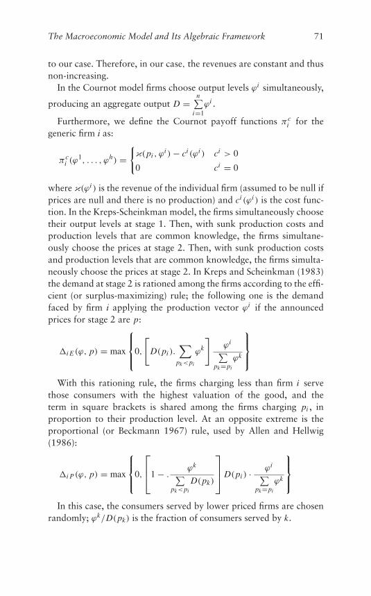
The Macroeconomic Model and Its Algebraic Framework 71
to our case. Therefore, in our case, the revenues are constant and thusnon-increasing.
In the Cournot model firms choose output levels ϕi simultaneously,
producing an aggregate output D =n∑
i=1ϕi .
Furthermore, we define the Cournot payoff functions πci for the
generic firm i as:
πci (ϕ
1, . . . , ϕh) ={
κ(pi , ϕi ) − ci (ϕi ) ci > 0
0 ci = 0
where κ(ϕi ) is the revenue of the individual firm (assumed to be null ifprices are null and there is no production) and ci (ϕi ) is the cost func-tion. In the Kreps-Scheinkman model, the firms simultaneously choosetheir output levels at stage 1. Then, with sunk production costs andproduction levels that are common knowledge, the firms simultane-ously choose the prices at stage 2. Then, with sunk production costsand production levels that are common knowledge, the firms simulta-neously choose the prices at stage 2. In Kreps and Scheinkman (1983)the demand at stage 2 is rationed among the firms according to the effi-cient (or surplus-maximizing) rule; the following one is the demandfaced by firm i applying the production vector ϕi if the announcedprices for stage 2 are p:
�i E (ϕ, p) = max
⎧⎪⎨⎪⎩0,
[D(pi ).
∑pk<pi
ϕk
]ϕi∑
pk=pi
ϕk
⎫⎪⎬⎪⎭With this rationing rule, the firms charging less than firm i serve
those consumers with the highest valuation of the good, and theterm in square brackets is shared among the firms charging pi , inproportion to their production level. At an opposite extreme is theproportional (or Beckmann 1967) rule, used by Allen and Hellwig(1986):
�i P (ϕ, p) = max
⎧⎪⎨⎪⎩0,
⎡⎢⎣1 − .ϕk∑
pk<pi
D(pk)
⎤⎥⎦ D(pi ) · ϕi∑pk=pi
ϕk
⎫⎪⎬⎪⎭In this case, the consumers served by lower priced firms are chosen
randomly; ϕk/D(pk) is the fraction of consumers served by k.
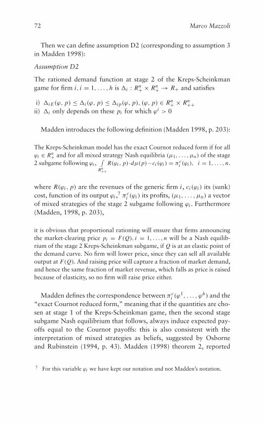
72 Marco Mazzoli
Then we can define assumption D2 (corresponding to assumption 3in Madden 1998):
Assumption D2
The rationed demand function at stage 2 of the Kreps-Scheinkmangame for firm i, i = 1, . . . , h is �i : Rn+ × Rn+ → R+ and satisfies
i) �i E (ϕ, p) ≤ �i (ϕ, p) ≤ �i p(ϕ, p), (ϕ, p) ∈ Rn+ × Rn++ii) �i only depends on these pi for which ϕi > 0
Madden introduces the following definition (Madden 1998, p. 203):
The Kreps-Scheinkman model has the exact Cournot reduced form if for allϕi ∈ Rn+ and for all mixed strategy Nash equilibria (μ1, . . . , μn) of the stage2 subgame following ϕi ,
∫Rn++
R(ϕi , p)·dμ(p)−ci (ϕi ) = πci (ϕi ), i = 1, . . . , n.
where R(ϕi , p) are the revenues of the generic firm i , ci (ϕi ) its (sunk)cost, function of its output ϕi ,7 πc
i (ϕi ) its profits, (μ1, . . . , μn) a vectorof mixed strategies of the stage 2 subgame following ϕi . Furthermore(Madden, 1998, p. 203),
it is obvious that proportional rationing will ensure that firms announcingthe market-clearing price pi = F(Q), i = 1, . . . , n will be a Nash equilib-rium of the stage 2 Kreps-Scheinkman subgame, if Q is at an elastic point ofthe demand curve. No firm will lower price, since they can sell all availableoutput at F(Q). And raising price will capture a fraction of market demand,and hence the same fraction of market revenue, which falls as price is raisedbecause of elasticity, so no firm will raise price either.
Madden defines the correspondence between πci (ϕ
1, . . . , ϕh) and the“exact Cournot reduced form,” meaning that if the quantities are cho-sen at stage 1 of the Kreps-Scheinkman game, then the second stagesubgame Nash equilibrium that follows, always induce expected pay-offs equal to the Cournot payoffs: this is also consistent with theinterpretation of mixed strategies as beliefs, suggested by Osborneand Rubinstein (1994, p. 43). Madden (1998) theorem 2, reported
7 For this variable ϕi we have kept our notation and not Madden’s notation.
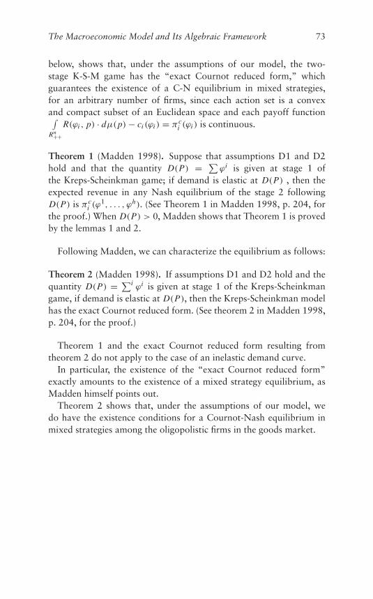
The Macroeconomic Model and Its Algebraic Framework 73
below, shows that, under the assumptions of our model, the two-stage K-S-M game has the “exact Cournot reduced form,” whichguarantees the existence of a C-N equilibrium in mixed strategies,for an arbitrary number of firms, since each action set is a convexand compact subset of an Euclidean space and each payoff function∫Rn++
R(ϕi , p) · dμ(p) − ci (ϕi ) = πci (ϕi ) is continuous.
Theorem 1 (Madden 1998). Suppose that assumptions D1 and D2hold and that the quantity D(P) = ∑
ϕi is given at stage 1 ofthe Kreps-Scheinkman game; if demand is elastic at D(P) , then theexpected revenue in any Nash equilibrium of the stage 2 followingD(P) is πc
i (ϕ1, . . . , ϕh). (See Theorem 1 in Madden 1998, p. 204, for
the proof.) When D(P) > 0, Madden shows that Theorem 1 is provedby the lemmas 1 and 2.
Following Madden, we can characterize the equilibrium as follows:
Theorem 2 (Madden 1998). If assumptions D1 and D2 hold and thequantity D(P) = ∑i
ϕi is given at stage 1 of the Kreps-Scheinkmangame, if demand is elastic at D(P), then the Kreps-Scheinkman modelhas the exact Cournot reduced form. (See theorem 2 in Madden 1998,p. 204, for the proof.)
Theorem 1 and the exact Cournot reduced form resulting fromtheorem 2 do not apply to the case of an inelastic demand curve.
In particular, the existence of the “exact Cournot reduced form”exactly amounts to the existence of a mixed strategy equilibrium, asMadden himself points out.
Theorem 2 shows that, under the assumptions of our model, wedo have the existence conditions for a Cournot-Nash equilibrium inmixed strategies among the oligopolistic firms in the goods market.

PART TWO
Model

3 A Computable Market Model: TheStructure of the Agent-BasedSimulation
MATTEO MORINI AND PIETRO TERNA
3.1 A Scheme to Start
Starting from the equation based construction introduced in Chapter2, we build now a macroeconomic simulation model of an economy,using the agent-based technique; the model is microfounded and soour explanation starts from the behavior of the agents and of themarket frameworks where they behave.
Agent-based simulation is a form of explicit modeling, so let uspoint out, with Epstein (2008), that:
Another advantage of explicit models is the feasibility of sensitivity analy-sis. One can sweep a huge range of parameters over a vast range of possiblescenarios to identify the most salient uncertainties, regions of robustness,and important thresholds. I don’t see how to do that with an implicitmental model. It is important to note that in the policy sphere (if not inparticle physics) models do not obviate the need for judgment. However,by revealing trade-offs, uncertainties, and sensitivities, models can disci-pline the dialogue about options and make unavoidable judgments moreconsidered.
Most of all, with Axtell (2000):
An agent-based model consists of individual agents, commonly implementedin software as objects. Agent objects have states and rules of behavior. Run-ning such a model simply amounts to instantiating an agent population,letting the agents interact, and monitoring what happens. That is, executingthe model – spinning it forward in time – is all that is necessary in order to“solve” it. Furthermore, when a particular instantiation of an agent-basedmodel, call it A, produces result R, one has established a sufficiency theo-rem, that is, the formal statement R if A (Newell and Simon, 1972, p. 13).
There are, ostensibly, several advantages of agent-based computationalmodeling over conventional mathematical theorizing. First, as describedabove, it is easy to limit agent rationality in agent-based computational
77
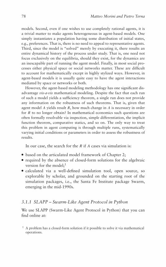
78 Matteo Morini and Pietro Terna
models. Second, even if one wishes to use completely rational agents, it isa trivial matter to make agents heterogeneous in agent-based models. Onesimply instantiates a population having some distribution of initial states,e.g., preferences. That is, there is no need to appeal to representative agents.Third, since the model is “solved” merely by executing it, there results anentire dynamical history of the process under study. That is, one need notfocus exclusively on the equilibria, should they exist, for the dynamics arean inescapable part of running the agent model. Finally, in most social pro-cesses either physical space or social networks matter. These are difficultto account for mathematically except in highly stylized ways. However, inagent-based models it is usually quite easy to have the agent interactionsmediated by space or networks or both.
However, the agent-based modeling methodology has one significant dis-advantage vis-a-vis mathematical modeling. Despite the fact that each runof such a model yields a sufficiency theorem, a single run does not provideany information on the robustness of such theorems. That is, given thatagent model A yields result R, how much change in A is necessary in orderfor R to no longer obtain? In mathematical economics such questions areoften formally resolvable via inspection, simple differentiation, the implicitfunction theorem, comparative statics, and so on. The only way to treatthis problem in agent computing is through multiple runs, systematicallyvarying initial conditions or parameters in order to assess the robustness ofresults.
In our case, the search for the R if A cases via simulation is:
● based on the articulated model framework of Chapter 2;● required by the absence of closed-form solutions for the algebraic
version for the model;1
● calculated via a well-defined simulation tool, open source, soexplorable by scholar, and grounded on the starting root of thesimulation packages, i.e., the Santa Fe Institute package Swarm,emerging in the mid-1990s.
3.1.1 SLAPP – Swarm-Like Agent Protocol in Python
We use SLAPP (Swarm-Like Agent Protocol in Python) that you canfind online at:
1 A problem has a closed-form solution if it possible to solve it via mathematicaloperations.
A Computable Market Model 79
● https://terna.github.io/SLAPP/ and● https://github.com/terna/SLAPP .
Boero et al. (2015) also describes SLAPP.The code of the agent-based model of this book is at:
● https://terna.github.io/oligopoly/ and● https://github.com/terna/oligopoly .
The code has a reference handbook, whose title is Oligopoly: theMaking of the Simulation Model,2 in compliance with the AEA DataAvailability Policy.3
Appendix C explains how to run the code, with some documentedexception for the different cases of Chapter 4.
3.1.2 The Structure of the Simulation Model
The structure of the simulation model is well represented via thesequence of the 12 items of Figure 3.1.
Following the circular sequence of the events, we can identify boththose related (i) to a conventional simple market aggregate clearingmechanism (SMAC) or (ii) to an atomistic simplified Hayekian market(ASHAM) interpretation of the price formation.
In SMAC, the aggregate production in quantity at time t is com-pared with the aggregate demand in value always at time t , to fixa clearing price, as in Section 3.8 (or, which is the same, in item 8 ofFigure 3.1), under the hypothesis that the unique good of the economyis a perishable one, so we have no warehouses and stocks.
In ASHAM, the interaction among sellers (the entrepreneurs) andbuyers (the workers and the entrepreneurs) is built via an atom-istic market where each agent meets her/his counterpart: this is theactivity described in Section 3.7 (or, which is the same, in item 7 ofFigure 3.1).
We work here in the perspective of a simplified Hayekian market; asuggested reading about Hayek is a quite recent paper of Bowles et al.(2017), with coauthors Alan Kirman and Rajiv Sethi.
2 https://github.com/terna/oligopoly/blob/master/Oligopoly.pdf .
3 https://www.aeaweb.org/journals/policies/data-availability-policy .
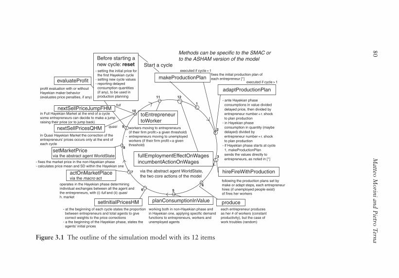
80M
atteoM
oriniandP
ietroT
erna
Before starting anew cycle: reset
evaluateProfit
nextSellPriceJumpFHM
nextSellPricesQHM
setMarketPricevia the abstract agent WorldState
actOnMarketPlacevia the macro act
setlnitialPricesHM planConsumptionInValue produce
hireFireWithProduction
adaptProductionPlan
Start a cycle- setting the initial price for the first Hayekian cycle- setting new cycle values- reporting delayed consumption quantities (if any), to be used in production planning
makeProductionPlan
toEntrepreneurtoWorker
fullEmploymentEffectOnWagesincumbentActionOnWages
Methods can be specific to the SMAC orto the ASHAM version of the model
executed if cycle = 1
- ante Hayekian phase consumptions in value divided delayed price, then divided by entrepreneur number + r. shock to plan production- in Hayekian phase consumption in quantity (maybe delayed) divided by entrepreneur number + r. shock to plan production- if Hayekian phase starts at cycle 1, makeProductionPlan sends the values directly to entrepreneurs, as noted in [*]
executed if cycle > 1
fixes the initial production plan ofeach entrepreneur [*]
following the production plans set bymake or adapt steps, each entrepreneurhires (if unemployed people exist)of fires her workers
each entrepreneur producesas her # of workers (constantproductivity), but the case ofwork troubles (random)
working both in non-Hayekian phase andin Hayekian one, applying specific demandfunctions to entrepreneurs, workers andunemployed agents
- at the beginning of each cycle states the proportion between entrepreneurs and total agents to give correct weights to the price corrections- a the beginning of the Hayekian phase, states the agents’ initial prices
operates in the Hayekian phase determiningindividual exchanges between all the agent andthe entrepreneurs, with (i) full and (ii) quasih. market
- fixes the market price in the non-Hayekian phase- calculates price mean and SD within the Hayekian one
in Quasi Hayekian Market the correction of theentrepreneurs’ prices occurs only at the end ofeach cycle
profit evaluation with or withoutHayekian maker behavior(evaluates price penalties, if any)
in Full Hayekian Market at the end of a cyclesome entrepreneurs can decide to make a jumpraising their price (or to jump back)
- workers moving to entrepreneurs (if their firm profit > a given threshold)- entrepreneurs moving to unemployed workers (if their firm profit < a given threshold)
via the abstract agent WorldState,the two core actions of the model
full
quasi
10
8
7
54
6
9
1211
3
2
1
Figure 3.1 The outline of the simulation model with its 12 items
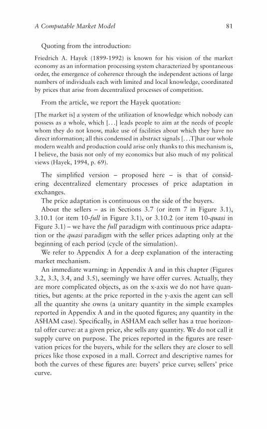
A Computable Market Model 81
Quoting from the introduction:
Friedrich A. Hayek (1899-1992) is known for his vision of the marketeconomy as an information processing system characterized by spontaneousorder, the emergence of coherence through the independent actions of largenumbers of individuals each with limited and local knowledge, coordinatedby prices that arise from decentralized processes of competition.
From the article, we report the Hayek quotation:
[The market is] a system of the utilization of knowledge which nobody canpossess as a whole, which [. . .] leads people to aim at the needs of peoplewhom they do not know, make use of facilities about which they have nodirect information; all this condensed in abstract signals [. . .T]hat our wholemodern wealth and production could arise only thanks to this mechanism is,I believe, the basis not only of my economics but also much of my politicalviews (Hayek, 1994, p. 69).
The simplified version – proposed here – is that of consid-ering decentralized elementary processes of price adaptation inexchanges.
The price adaptation is continuous on the side of the buyers.About the sellers – as in Sections 3.7 (or item 7 in Figure 3.1),
3.10.1 (or item 10-full in Figure 3.1), or 3.10.2 (or item 10-quasi inFigure 3.1) – we have the full paradigm with continuous price adapta-tion or the quasi paradigm with the seller prices adapting only at thebeginning of each period (cycle of the simulation).
We refer to Appendix A for a deep explanation of the interactingmarket mechanism.
An immediate warning: in Appendix A and in this chapter (Figures3.2, 3.3, 3.4, and 3.5), seemingly we have offer curves. Actually, theyare more complicated objects, as on the x-axis we do not have quan-tities, but agents: at the price reported in the y-axis the agent can sellall the quantity she owns (a unitary quantity in the simple examplesreported in Appendix A and in the quoted figures; any quantity in theASHAM case). Specifically, in ASHAM each seller has a true horizon-tal offer curve: at a given price, she sells any quantity. We do not call itsupply curve on purpose. The prices reported in the figures are reser-vation prices for the buyers, while for the sellers they are closer to sellprices like those exposed in a mall. Correct and descriptive names forboth the curves of these figures are: buyers’ price curve; sellers’ pricecurve.
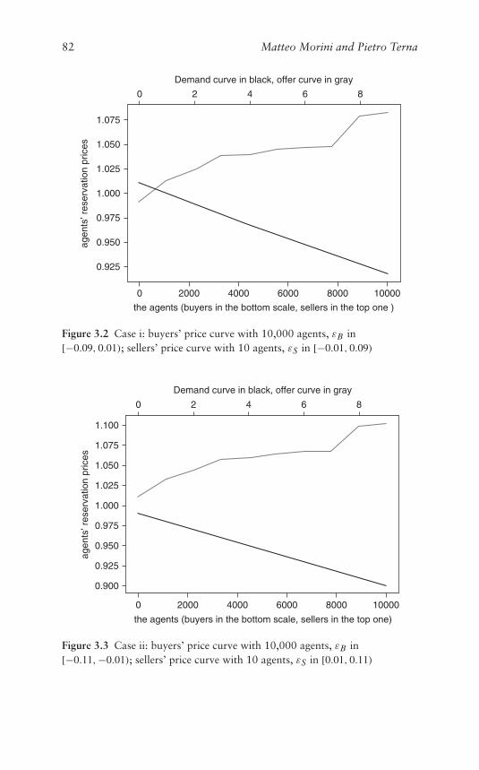
82 Matteo Morini and Pietro Terna
0 2000 4000 6000 8000 10000
the agents (buyers in the bottom scale, sellers in the top one )
0.925
0.950
0.975
1.000
1.025
1.050
1.075
agen
ts’ r
eser
vatio
n pr
ices
0 2 4 6 8
Demand curve in black, offer curve in gray
Figure 3.2 Case i: buyers’ price curve with 10,000 agents, εB in[−0.09, 0.01); sellers’ price curve with 10 agents, εS in [−0.01, 0.09)
0 2000 4000 6000 8000 10000
the agents (buyers in the bottom scale, sellers in the top one)
0.900
0.925
0.950
0.975
1.000
1.025
1.050
1.075
1.100
agen
ts’ r
eser
vatio
n pr
ices
0 2 4 6 8
Demand curve in black, offer curve in gray
Figure 3.3 Case ii: buyers’ price curve with 10,000 agents, εB in[−0.11,−0.01); sellers’ price curve with 10 agents, εS in [0.01, 0.11)
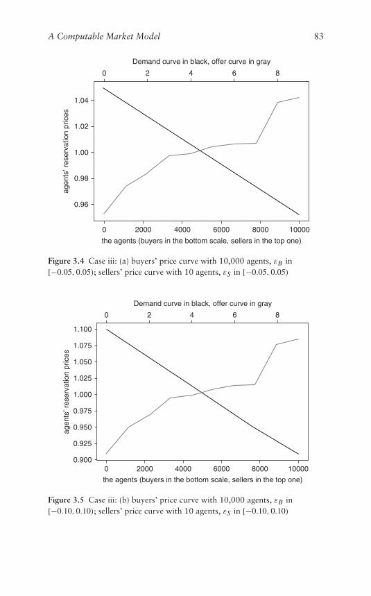
A Computable Market Model 83
0 2000 4000 6000 8000 10000
the agents (buyers in the bottom scale, sellers in the top one)
0.96
0.98
1.00
1.02
1.04
agen
ts’ r
eser
vatio
n pr
ices
0 2 4 6 8
Demand curve in black, offer curve in gray
Figure 3.4 Case iii: (a) buyers’ price curve with 10,000 agents, εB in[−0.05, 0.05); sellers’ price curve with 10 agents, εS in [−0.05, 0.05)
0 2000 4000 6000 8000
the agents (buyers in the bottom scale, sellers in the top one)
0.900
0.925
0.950
0.975
1.000
1.025
1.050
1.075
1.100
agen
ts’ r
eser
vatio
n pr
ices
0 2 4 6 8
Demand curve in black, offer curve in gray
10000
Figure 3.5 Case iii: (b) buyers’ price curve with 10,000 agents, εB in[−0.10, 0.10); sellers’ price curve with 10 agents, εS in [−0.10, 0.10)

84 Matteo Morini and Pietro Terna
The following sections help us understand the items of Figure 3.1;to deepen how the different items are linked among them, it is possibleto have a look to the reference handbook: The Oligopoly Project: TheMaking of the Simulation Model.4
The sequence of the items of the figure are also related to theexplanation in Section C.1.
3.1.3 What Is a Cycle and What Are Sub-Steps?
How the time operates: each cycle of 12 steps, as described in Figure3.1, is equivalent to a step ahead of the time counter t .
The number of cycles of the simulation is reported in the variablenCycle, as in Appendix B.
In ASHAM, the item 7 as in Section 3.7 is subdivided in sub-steps.As explained in n the reference handbook The Oligopoly Project:
The Making of the Simulation Model, the sequence of the events ismanaged by a schedule mechanism, defining steps and sub-steps.
Firms produce a unique kind of good.
3.1.4 Item 1: Reset Action
We refer to item 1 in Figure 3.1.Before starting a new cycle, we have to run a reset action. The
reset action acts once in each simulation cycle, because in our caseis related only to common variables of the simulation. The agent exe-cuting the cleaning operation is that with the identifier (the variablenumber) equal to 1. If no agent has that identifier, all will be acting,with not useful repetitions of the same task.5
3.2 Item 2: makeProductionPlan or adaptProductionPlan
3.2.1 makeProductionPlan
We refer to item 2 in Figure 3.1.
4 Online at https://github.com/terna/oligopoly/blob/master/Oligopoly.pdf.
5 For technical details, look at the section “The Scheduling Mechanism at theLevel of the Model” in the reference handbook Oligopoly: The Making of theSimulation Model.
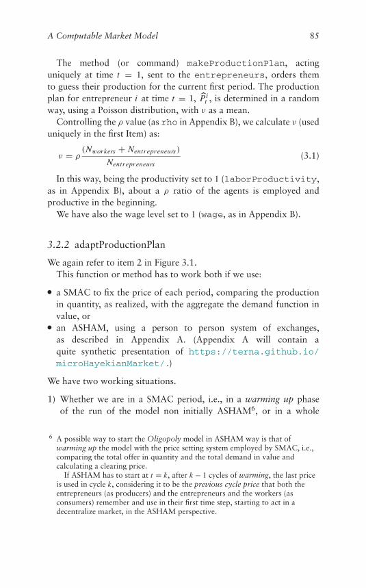
A Computable Market Model 85
The method (or command) makeProductionPlan, actinguniquely at time t = 1, sent to the entrepreneurs, orders themto guess their production for the current first period. The productionplan for entrepreneur i at time t = 1, P̂ i
t , is determined in a randomway, using a Poisson distribution, with ν as a mean.
Controlling the ρ value (as rho in Appendix B), we calculate ν (useduniquely in the first Item) as:
ν = ρ(Nworkers + Nentrepreneurs)
Nentrepreneurs(3.1)
In this way, being the productivity set to 1 (laborProductivity,as in Appendix B), about a ρ ratio of the agents is employed andproductive in the beginning.
We have also the wage level set to 1 (wage, as in Appendix B).
3.2.2 adaptProductionPlan
We again refer to item 2 in Figure 3.1.This function or method has to work both if we use:
● a SMAC to fix the price of each period, comparing the productionin quantity, as realized, with the aggregate the demand function invalue, or
● an ASHAM, using a person to person system of exchanges,as described in Appendix A. (Appendix A will contain aquite synthetic presentation of https://terna.github.io/microHayekianMarket/ .)
We have two working situations.
1) Whether we are in a SMAC period, i.e., in a warming up phaseof the run of the model non initially ASHAM6, or in a whole
6 A possible way to start the Oligopoly model in ASHAM way is that ofwarming up the model with the price setting system employed by SMAC, i.e.,comparing the total offer in quantity and the total demand in value andcalculating a clearing price.
If ASHAM has to start at t = k, after k − 1 cycles of warming, the last priceis used in cycle k, considering it to be the previous cycle price that both theentrepreneurs (as producers) and the entrepreneurs and the workers (asconsumers) remember and use in their first time step, starting to act in adecentralize market, in the ASHAM perspective.
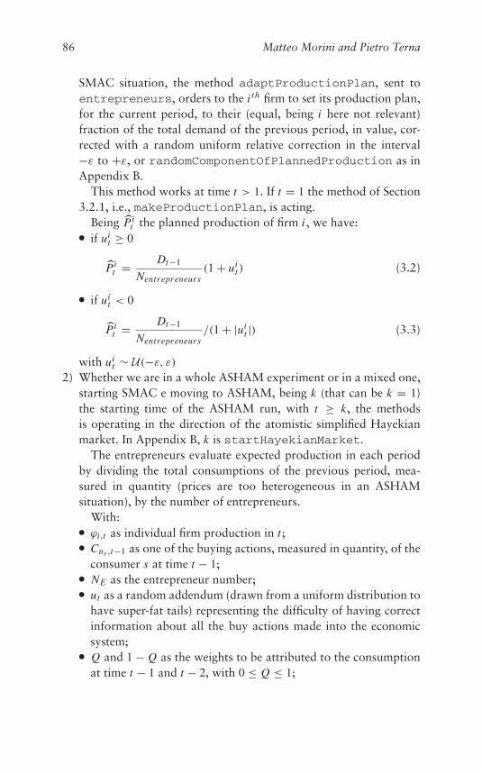
86 Matteo Morini and Pietro Terna
SMAC situation, the method adaptProductionPlan, sent toentrepreneurs, orders to the i th firm to set its production plan,for the current period, to their (equal, being i here not relevant)fraction of the total demand of the previous period, in value, cor-rected with a random uniform relative correction in the interval−ε to +ε, or randomComponentOfPlannedProduction as inAppendix B.
This method works at time t > 1. If t = 1 the method of Section3.2.1, i.e., makeProductionPlan, is acting.
Being P̂it the planned production of firm i , we have:
● if uit ≥ 0
P̂it = Dt−1
Nentrepreneurs(1 + ui
t ) (3.2)
● if uit < 0
P̂it = Dt−1
Nentrepreneurs/(1 + |ui
t |) (3.3)
with uit ∼ U(−ε, ε)
2) Whether we are in a whole ASHAM experiment or in a mixed one,starting SMAC e moving to ASHAM, being k (that can be k = 1)the starting time of the ASHAM run, with t ≥ k, the methodsis operating in the direction of the atomistic simplified Hayekianmarket. In Appendix B, k is startHayekianMarket.
The entrepreneurs evaluate expected production in each periodby dividing the total consumptions of the previous period, mea-sured in quantity (prices are too heterogeneous in an ASHAMsituation), by the number of entrepreneurs.
With:● ϕi,t as individual firm production in t ;● Cns ,t−1 as one of the buying actions, measured in quantity, of the
consumer s at time t − 1;● NE as the entrepreneur number;● ut as a random addendum (drawn from a uniform distribution to
have super-fat tails) representing the difficulty of having correctinformation about all the buy actions made into the economicsystem;
● Q and 1 − Q as the weights to be attributed to the consumptionat time t − 1 and t − 2, with 0 ≤ Q ≤ 1;
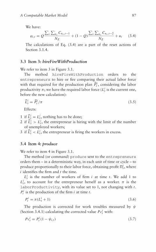
A Computable Market Model 87
We have:
ϕi,t = Q
∑s∑
nsCns ,t−1
NE+ (1 − Q)
∑s∑
nsCns ,t−2
NE+ ut (3.4)
The calculations of Eq. (3.4) are a part of the reset actions ofSection 3.1.4.
3.3 Item 3: hireFireWithProduction
We refer to item 3 in Figure 3.1.The method hireFireWithProduction orders to the
entrepreneurs to hire or fire comparing their actual labor forcewith that required for the production plan P̂i
t , considering the laborproductivity π ; we have the required labor force (Li
t is the current one,before the new calculation):
L̂it = P̂i
t /π (3.5)
Effects:
1 if L̂it = Li
t , nothing has to be done;2 if L̂i
t > Lit , the entrepreneur is hiring with the limit of the number
of unemployed workers;3 if L̂i
t < Lit , the entrepreneur is firing the workers in excess.
3.4 Item 4: produce
We refer to item 4 in Figure 3.1.The method (or command) produce sent to the entrepreneurs
orders them – in a deterministic way, in each unit of time or cycle – toproduce proportionally to their labor force, obtaining profit �i
t , wherei identifies the firm and t the time.
Lit is the number of workers of firm i at time t . We add 1 to
Lit , to account for the entrepreneur herself as a worker. π is the
laborProductivity, with its value set to 1, not changing with t .Pi
t is the production of the firm i at time t .
Pit = π(Li
t + 1) (3.6)
The production is corrected for work troubles measured by ψ
(Section 3.4.1) calculating the corrected value Pcit with:
Pcit = Pi
t (1 − ψi,t ) (3.7)
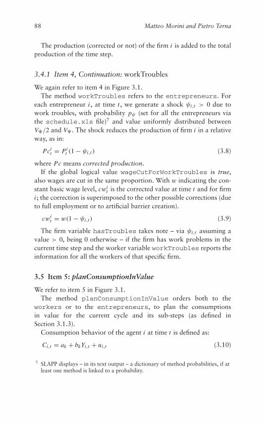
88 Matteo Morini and Pietro Terna
The production (corrected or not) of the firm i is added to the totalproduction of the time step.
3.4.1 Item 4, Continuation: workTroubles
We again refer to item 4 in Figure 3.1.The method workTroubles refers to the entrepreneurs. For
each entrepreneur i , at time t , we generate a shock ψi,t > 0 due towork troubles, with probability pψ (set for all the entrepreneurs viathe schedule.xls file)7 and value uniformly distributed betweenV�/2 and V� . The shock reduces the production of firm i in a relativeway, as in:
Pcit = Pi
t (1 − ψi,t ) (3.8)
where Pc means corrected production.If the global logical value wageCutForWorkTroubles is true,
also wages are cut in the same proportion. With w indicating the con-stant basic wage level, cwi
t is the corrected value at time t and for firmi ; the correction is superimposed to the other possible corrections (dueto full employment or to artificial barrier creation).
cwit = w(1 − ψi,t ) (3.9)
The firm variable hasTroubles takes note – via ψi,t assuming avalue > 0, being 0 otherwise – if the firm has work problems in thecurrent time step and the worker variable workTroubles reports theinformation for all the workers of that specific firm.
3.5 Item 5: planConsumptionInValue
We refer to item 5 in Figure 3.1.The method planConsumptionInValue orders both to the
workers or to the entrepreneurs, to plan the consumptionsin value for the current cycle and its sub-steps (as defined inSection 3.1.3).
Consumption behavior of the agent i at time t is defined as:
Ci,t = ak + bkYi,t + ui,t (3.10)
7 SLAPP displays – in its text output – a dictionary of method probabilities, if atleast one method is linked to a probability.
A Computable Market Model 89
with ui,t from u ∼ N (0, sd).8
The individual i can be:
1 an entrepreneur, with Yi,t = prof i ti,t−1 + wage;2 an employed worker, with Yi,t = wage and the special9 case Yi,t =
wcit , with wci
t defined in Eq. (3.9);3 an unemployed workers,10 with Yi,t = socialWelfareCompensation.
The ak and bk values are set via the parameters of the model. Weuse socialWelfareCompensation as in Appendix B.
Finally, a quota of the unspent consumption capability com-ing from the past, is added to the result. The quota, with avalue in the interval [0, 1], has value qres , and it is appliedto reUseUnspentConsumptionCapability as in Appendix B,giving:
C+i,t = Ci,t + qres · unspentConsumptionCapabili t y (3.11)
Referring to the planned consumption in value in a time step, themethod updates that value only until the starting point of ASHAM, soin SMAC phase, if any.
In the ASHAM phase, in each sub-step of a cycle (look at Sec-tion 3.1.3) we establish a max quantity of consumptions, via a quotaintroduced interactively in the starting session of the simulation (vari-able consumptionQuota, as in Appendix B). This action mimics thebehavior of the households within each time period.
When ASHAM operates, the consumption total amount comes fromsumming up all the consumption actions generated by this (item 5)method.
3.6 Item 6: setInitialPricesHM
We refer to item 6 in Figure 3.1.The method (or command) setInitialPricesHM, sent to all,
operates only in the ASHAM phase of each run.The method performs several actions.
8 With sd value reported by the parameter consumptionRandomComponentSD.9 Activated if the common value wageCutForWorkTroubles is true.
10 In this case, if the random component exceeds the consumption coming fromsocial welfare compensation, we can have negative consumption; in case,consumption is set to 0.
90 Matteo Morini and Pietro Terna
1) In each cycle, while the ASHAM is working, the method calcu-lates the ratio Z = number of sellers
number of buyers between sellers and buyers asrequested in adopting the ASHAM paradigm: the modification ofthe prices is continuous, both on the side of the buyers (all theagents) and of the side of the sellers (the entrepreneurs); the fre-quencies of the modifications belong to two highly different scalesand as a consequence the amplitude of the price corrections arevery different.
2) In the first step of the ASHAM phase, the method states the initialcommon price: being at time k, we use as starting point the price attime k − 1 or, if k > 2, at k − 2. The double lagged price correctionis justified because we are considering the production decisions attime t as based on the decisions of consumption at t − 1, relatedto the income at time t − 1; these decisions are made before thedetermination of the prices at t − 1 (in the SMAC scheme emergesonly when comparing the demand and the predetermined offer).If we want to evaluate the consumption in quantity, without theeffect of a too limited or too abundant offer, we have to use t − 2prices. This construction is eliminated with ASHAM interaction ofbuyers and sellers in a dispersed way.
If k = 1, we use the SMAC structure market, calculating the priceas the equilibrium price that would have been created at t = 1 inthe SMAC execution, but avoiding the random shocks of item 8 inSection 3.8.
3) Calculation of the individual starting prices. The parameters in usehere are initShock and initShift. Here we calculate boththe individual buyPrice and the individual sellPrice, becauseeach agent can act both as entrepreneur-seller and as buyer.● We add random corrections to both the types of initial prices;
so, we will start the first cycle of the simulation with two ini-tial distributions of values for the buyers and for the sellers.Let initShock be the variable containing the relative value ι
as range of the correction of the individual starting prices in arandom uniform way, with the internal variable initShift,having value ν, reasonably11 in the interval [−1, 1], e.g., 0.10,shifting the range of the whole correction.
11 With very different effects.
A Computable Market Model 91
Our goal here is that of initializing (i) buyer prices mostlybelow/above the starting price and (ii) seller prices mostlyabove/below the starting price, to induce more or less intensivelythe necessity of individual price corrections from the beginningof the exchanges.12
With pS,i as initial sell price of agent i , pB,i as initial buy price ofagent i and pH as starting ASHAM price, we have the followingequations:● if εS,i ≥ 0
pS,i = pH (1 + εS,i ) (3.12)
● if εS,i < 0
pS,i = pH/(1 + |εS,i |) (3.13)
with εS,i ∼ U(−ν ι, (1 − ν) ι). Also,● if εB,i ≥ 0
pB,i = pH (1 + εB,i ) (3.14)
● if εB,i < 0
pB,i = pH/(1 + |εB,i |) (3.15)
with εB,i ∼ U(−(1 − ν) ι, ν ι).i) If we adopt ν = 0.10 and ι = 0.10, we only have a quite
small overlapping of the initial price correction (correctionare never too rational, with someone moving in the wrongdirection). The ε corrections will be uniformly distributedbetween −0.01 and 0.09 for the sellers and between −0.09and 0.01 for the buyers.Considering the individual prices as reservation prices, wehave a buyers’ price and sellers’ price curves crossing on theleft side of their graphic representation, as in Figure 3.2.
ii) If we want not overlapping curves, we can use ν < 0, e.g.,ν = −0.1, with ι = 0.10. The ε corrections will be uniformly
12 At creation time, for each agent sellPrice is set to 1,000 and buyPrice to−1,000, as implausible values, not operational.
In any case, the sellers (entrepreneur) cannot operate into the ASHAM untiltheir starting price is defined; this information is reported setting to (True) theagent’s variable sellPriceDefined.
92 Matteo Morini and Pietro Terna
distributed between 0.01 and 0.11 for the sellers and between−0.11 and −0.01 for the buyers, as in Figure 3.3.
iii) We can also choose to start in a balancing situation, with ν =0.5 and, e.g., ι = 0.10|0.20. ε corrections will be uniformlydistributed(a) between −0.05 and 0.05 for the sellers and between −0.05and 0.05 for the buyers, as in Figure 3.4 for ι = 0.10,or (b) between −0.10 and 0.10 for the sellers and between−0.10 and 0.10 for the buyers, as in Figure 3.5 for ι = 0.20,doubling the y scale.
We generate symmetric effect both for positive and negative ratesof change, using the so-called rational discount rule, with a simplestructure such as:● if the rate of change i ≥ 0, xc (i.e., x after the correction) is
xc = x(1 + i) (3.16)
● if the rate of change i < 0, xc (i.e., x after the correction) is
xc = x/(1 + i) (3.17)
3.7 Item 7: actOnMarketPlace
We refer to item 7 in Figure 3.1.The method operates only in the ASHAM phase of each run.Both the entrepreneurs and the workers are buyers, while the
sellers are uniquely the entrepreneurs.The following is the sequence of the actions.
● The method is repeating its action several times in each cycle, foreach sub-step (about sub-steps in cycles, look at the Section 3.1.3).
Technically, sub-steps are included in a macro and the number ofrepetitions for each buyer in each cycle (the number of buy attempts)is regulated by the number of repetitions into the macro.13 In eachrepetition, the program shuffles the agents. Each agent has in mem-ory the effect of the action done in the previous repetition within acycle.
13 See https://github.com/terna/oligopoly/blob/master/Oligopoly.pdf for the reference handbook The Oligopoly Project: TheMaking of the Simulation Model.

A Computable Market Model 93
The number of sub-steps is incremented to cope with thephenomenon of the idle agents reported in Section A.5 ofAppendix A.
● Search for sellers. In the first sub-step of each multiple call of themethod in each cycle, and for each buyer, a seller is chosen from atemporary list of sellers having still unsold products.
● Sold products are recorded in each sub-step and reset to 0 when anew cycle starts.
The deal between a buyer and a seller is based on the confronta-tion of the prices. Considering the buy price of agent i and the sellprice of agent j , if pB,i � pS, j the agents exchange, at the sellerprice, the minimum quantity between (i) the buying capacity of thebuyer at that price, i.e., its maximum spending value in each stepof a cycle at that price,14 and (ii) the actual production residualquantity of the seller.
The revenue of the seller (one of the entrepreneurs) isaccounted for profit calculations.
● Prices: what price in each action for each agent?
– The best is their price, i.e., the price at which they have concludeda deal (the last one, if more than a deal were made in a same timeinterval)15 or that of the last bid (if buyers) or ask (if sellers) theymade without concluding a deal. This price is corrected with therules below.
– To generate symmetric effect both for positive and negative ratesof change, we apply a symmetric rational calculation, as describedin Section 3.5. Missing this device, or trick, the cumulative effectof negative and positive corrections would always be negative.16
– The continuous process of correction of the individual prices,applied to the transactions within each cycle, works in thefollowing way.
1) We modify the buy price (a random correction) if the last agentnegotiation, also if unsuccessful, was on the buy side.
14 As stated in Section 3.5, in each step of a cycle, we establish a maximumquantity of consumptions, via a quota introduced interactively in the startingsession of the program.
15 The event is possible if the agents buy or sell only fractions of their buying orselling quantities, thus repeating their actions.
16 x(1 − i)(1 + 1) = x(1 − i2) < x .
94 Matteo Morini and Pietro Terna
2) The same is true for the sell price, but here only in caseof hParadigm (as in Appendix B) set to full (see Sec-tion 3.1 and Section 3.6); if this is the case, the sellers’price correction is limited by the factor Z reporting thevalue of ratioSellersBuyers, to account for the differ-ent (extremely higher) number of corrections they made in acycle.Consider now price correction as running shocks calculatedwith a shift upon or below the 0; the values are different forbuyers and sellers with runningShockB, runningShiftBand runningShockS, runningShiftS (as in Appendix B).Let runningShock B or S be the internal variable containingthe relative value ι̃ (e.g., 0.05) as the range of the correction orthe individual running prices in a random uniform way (butshifted, with the internal variable runningShift B or S con-taining the value of ν̃ defined in the interval [0, 0.5], e.g., 0.10,having in case a quite low effect below, for the sellers, andabove, for the buyers, the 0), with pB,i as buy price of agent iand pS,i as sell price of agent i .
The equations are the same as 3.12, 3.13, 3.14, and 3.15, with ν̃B
or ν̃S substituting ν and ι̃B or ι̃S substituting ι. Remember Z , theratio of sellers to buyers.
● After the starting cycle of the ASHAM phase, the agents use twostatus variables (technically: statusB and statusS), initialized to0 and reporting their short-term history both as buyers (workers orentrepreneurs) and as sellers (entrepreneurs).Conventions:– self.statusB
◦ 0 means never used;◦ 1 if previous action was a successful buy attempt;◦ −1 if previous action was an unsuccessful buy attempt.
– self.statusS
◦ 0 means never used;◦ 1 if previous action was a successful sell attempt;◦ −1 if previous action was an unsuccessful sell attempt.
– Buyer case:◦ if the last transaction succeeded (statusB = 1) and εBdown ,i ≥ 0:
pB,i t = pB,i t−1(1 + εBdown ,i ) (3.18)
A Computable Market Model 95
◦ if the last transaction succeeded (statusB = 1) and εBdown ,i < 0:
pB,i t = pB,i t−1/(1 + |εBdown ,i |) (3.19)
with εBdown ,i ∼ U(−(1 − ν̃B) ι̃B, ν̃B ι̃B), so mostly negative (theagent tries to decrease its reservation price);
◦ if the last transaction failed (statusB = 1) and εBup,i ≥ 0:
pB,i t = pB,i t−1(1 + εBup,i ) (3.20)
◦ if the last transaction failed (statusB = −1) and εBup,i < 0:
pB,i t = pB,i t−1/(1 + |εBup,i |) (3.21)
with εBup,i ∼ U(−ν̃B ι̃B, (1 − ν̃B) ι̃B), so mostly positive (theagent tries to increase its reservation price).
– Seller case:17
◦ if the last transaction succeeded (statusS = 1) and εSup,i ≥ 0:
pS,i t = pS,i t−1(1 + ZεSup,i ) (3.22)
◦ if the last transaction succeeded (statusS = 1) and εSup,i < 0:
pS,i t = pS,i t−1/(1 + Z |εSup,i |) (3.23)
with εSup,i ∼ U(−ν̃S ι̃S, (1−ν̃S) ι̃S), so mostly positive (the agenttries to increase its reservation price);
◦ if the last transaction failed (statusS = −1) and εSdown ,i ≥ 0:
pS,i t = pS,i t−1(1 + ZεSdown ,i ) (3.24)
◦ if the last transaction failed (statusS = −1) and εSdown ,i < 0:
pS,i t = pS,i t−1/(1 + Z |εSdown ,i |) (3.25)
with εSdown ,i ∼ U(−(1 − ν̃S) ι̃S, ν̃S ι̃S), so mostly negative (theagent tries to decrease its reservation price).
– The rational calculation introduced in Section 3.6 is applied hereto the couples of eqs.: (3.18) or (3.19); (3.20) or (3.21); (3.22) or(3.23); (3.24) or (3.25).
17 Operating in case of hParadigm (as in Appendix B) set to full; if set to quasithe correction is made once per cycle; if the parameter is set to a value, whichis neither full nor quasi, we have a side effect, because no corrections willhappen on sell prices. In the case of the quasi scheme, in the first cycle the fullscheme is anyway operating, see Section 3.10.2.
96 Matteo Morini and Pietro Terna
– The method actOnMarketPlace also has a tool to gener-ate an optional report about residual consumption in valueand unsold production in quantity, at the beginning ofeach sub-step in a cycle. To obtain the report, the variablecheckResConsUnsoldProd (as in Appendix B) has to be true.The report is printed in the regular output flow of the model.
3.8 Item 8: setMarketPrice
We refer to item 8 in Figure 3.1.The method setMarketPrice orders to the abstract agent
WorldState to evaluate the market clearing prices in a SMAC sit-uation or simply to record the mean and the standard deviation of theprices in each cycle of an ASHAM.
In agent-based model, usually the agents are mimicking an actualsubject existing in the reality; in this case, we have an abstract agentmaking computations both (i) relevant from a theoretical economicpoint of view or (ii) simply accounting statistical data.
Considering (ii) in the SMAC case, the method evaluates the marketclearing price, considering each agent behavior plus an external shock,potentially large.
We introduce a shock ! uniformly distributed between −Land +L, where L is a rate on base 1, e.g., 0.10, defined asmaxDemandRelativeRandomShock in Appendix B. To keep theeffect as symmetric, we have the following equations determining thelearing price:
if the shock ! is (≥ 0):
pt = Dt (1 + !)
Ot(3.26)
if the shock ! is (< 0):
pt = Dt/(1 + !)
Ot(3.27)
with pt clearing market price at time t ; Dt demand in value18 at timet ; Ot offer in quantity19 at time t .
18 Generated by the agent entrepreneurs and workers as in Section 3.5.19 Generated by the agent entrepreneurs as in Section 3.4.
A Computable Market Model 97
3.9 Item 9: evaluateProfit
We refer to item 9 in Figure 3.1.The method orders to the entrepreneurs to calculate their prof-
its, using Pit , the production, and Li
t , the labor force, plus 1 to accountfor the entrepreneur herself.
The use of Pit , the actual production of the entrepreneurs, accounts
both for the production plan decided with adaptProductionPlan,Section 3.2, and for the limits in hiring, if any, in hireFireWithProduction, Section 3.3. The sum of all the actual productions of eachentrepreneur is used, as in Section 3.8, in setMarketPrice.
pt is the price, coming from the analysis of Section 3.7 forASHAM, or 3.8 for SMAC.
w is the wage per employee and time unit, set to 1.0 in these researchand not changing with t , but the case of the important events of:
● wage rise due both to full employment (Section 3.12.1), and● to the creation of barriers against new entrants (Section 3.12.2).
C are extra costs for new entrant firms. They are calibrated to assurethe effectiveness of the action described in Section 3.12.2, but in a nonrigid way, thanks to the movements in prices.
If the variable wageCutForWorkTroubles (as in Appendix B) isset to True, the costs determination takes in account the reduction ofthe wages (but the wage of the entrepreneur, not changing).
Considering the presence of work troubles (see Section 3.4.1),the determination of the clearing price, as at page 96, can sig-nal an increase in the equilibrium price, due to the lackingproduction.
The (relative) shock ψi,t > 0 due to work troubles is defined inSection 3.4.1.
Within the SMAC paradigm, in the presence of work troubles thefirm has to accept a reduction of its price, to compensate its customersfor having undermined the confidence in the implicit commitment ofproducing a given quantity (the production plan, specified in Sec-tion 3.2.1). The penalty value, as a relative measure, is reported inpenaltyValue (as in Appendix B) and here shortly as pv. Locally,pvi
t , for the firm i at time t , is set to pv if ψi,t > 0; otherwise (ψi,t = 0)is set to 0.
98 Matteo Morini and Pietro Terna
Eqs. (3.28) and (3.29) are used in the SMAC context, while Eqs.(3.30) and (3.31) work in the ASHAM one.
The profit evaluation in SMAC, if wageCutForWorkTroubles isset to True, is:
�it = pt (1 − pv1
t )Pit − (w − ψi,t )(L
it − 1) − 1w − C (3.28)
being 1w the wage of the entrepreneur.If wageCutForWorkTroubles is set to False, the result is:
�it = pt (1 − pvi
t )Pit − wLi
t − C (3.29)
In ASHAM we have, with REV it reporting the revenue of firm i at
time t , and wageCutForWorkTroubles set to True:
�it = REV i
t − (w − ψi,t )(Lit − 1) − 1w − C (3.30)
being 1w the wage of the entrepreneur.If wageCutForWorkTroubles is set to False, the result is:
�it = REV i
t − wLit − C (3.31)
The experiments run in April 2017 (with V5 of this method) for thefinal version for the Italian Economic Journal have the penalty valuepvi
t set to 0.The new entrant firms have extra costs C to be supported, retrieved
in XC variables, but only for k periods, as stated in commonVar.pyand activated by method toEntrepreneur.
3.10 Item 10: nextSellPriceJumpFHM andnextSellPricesQHM
The methods nextSellPriceJumpFHM and nextSellPricesQHMare related to ASHAM and work in two different perspectives: thefirst method, in the full ASHAM case, with the sellers – as the buy-ers – changing continuously their prices and sometimes adjusting themin an extraordinary way (with a jump); the second one, in the quasiASHAM case, where the sellers change their prices only once in eachtime period, in the beginning.
3.10.1 Item 10–full: nextSellPriceJumpFHM
We refer to item 10-full in Figure 3.1.

A Computable Market Model 99
The method nextSellPriceJumpFHM operates only in theASHAM context. It works modifying the sell price of a spe-cific entrepreneur-seller with jump-up corrections of her reserva-tion prices. The method operates with a given probability. Thesettings are the jump size and the pJump probability (as inAppendix B).jump is a relative value, so pJ = p(1 + jump).The probability of jumping operates as a switch, moving the agent
to be a jumper and vice versa.If a worker of a jumping-up entrepreneur moves to be an
entrepreneur herself, she starts as a jumper.In the full-case (as described in Section 3.7), with the use of jump,
an entrepreneur making a jump continues anyway to modify her pricewithin the actOnMaketPlaceMethod in each sub-step (as definedin Section 3.1.3).
3.10.2 Item 10–quasi: nextSellPricesQHM
We refer to item 10-quasi in Figure 3.1.The method nextSellPricesQHM operates in the ASHAM con-
text and specifically in the quasi case (as described in Section 3.7).In this case, with the price correction switch hParadigm set to
quasi, the correction of the entrepreneurs’ prices occurs only at theend of each cycle.20
We have several possible choices. To select an option we use thevariable quasiHchoice (as in Appendix B) with possible values:unsold, profit, and randomUp.
i) Case quasiHchoice set to unsold. We compare sold productionproduction ,
as sold-ratio, with two thresholds:● soldThreshold121 and● soldThreshold222, both in Appendix B;● if the result is less or equal than soldThreshold1,
a random correction is applied, dividing the price by
20 In this case, it could be important to start with a well-balanced initial situation,as in solution (iii) in Section 3.6.
21 E.g., 0.90.22 E.g., 0.99.
100 Matteo Morini and Pietro Terna
1 + |u1|, with u1 drawn from a flat distribution u1 ∼U(decreasingRateRange, 0);23
● if the result is greater or equal than soldThreshold2,a random correction is applied, multiplying the price by1 + u2 with u2 drawn from a flat distribution u2 ∼U(0, increasingRateRange);24
● between the soldThreshold1 and soldThreshold2 values,no corrections occur;
● if entrepreneursMindIfPlannedProductionFalls isTrue and (Section 3.2.2) the planned production is falling morethan a given threshold,25 the entrepreneurs (individually) reducetheir prices, with the same mechanism above; this conditionsupersede the confrontation of the sold-ratio with the twothresholds.
ii) Case quasiHchoice set to randomUp. The logical scheme is thesame of the jump in Section 3.10.1 for the full implementation, buthere the huge difference is that we have no corrections within thespecific cycle, with the jumped or un-jumped price kept constant.
We use the same parameters of Section 3.10.1, so the jump sizewith the pSize probability (as in Appendix B).jump is a relative value, so pJ = p(1 + jump).
The probability of jumping operates as a switch, moving theagent to be a jumper and vice versa. If a worker of a jumping upentrepreneur moves to be an entrepreneur herself, she starts as ajumper.
In the quasi-case (as described in Section 3.7), with the use ofjump, an entrepreneur making a jump will keep unchanged theprice for a whole cycle (or more, if the opposite action is notturning up).
iii) Case quasiHchoice set to profit. The entrepreneur decidesto raise or to lower her price if the profit is negative.priceSwitchIfProfitFalls is a switch with values “raise”or “lower.” To summarize the actual difficulty of knowing thedemand elasticity, the actual choice between raising or low-ering the price is a random one, with 60% of probability
23 E.g., decreasingRateRange = −0.10.24 E.g., increasingRateRange = 0.01.25 thresholdToDecreaseThePriceIfTotalPlannedPFalls, e.g., 0.05 (Appendix B).
A Computable Market Model 101
to the first choice (“raise”) and 40% to the other one ifpriceSwitchIfProfitFalls is set to “raise”; vice versa, if itset to “lower.” The correction is made with probability pJump26
defined as above and size jump, again as above (both in AppendixB), calculating:
pP = p(1 + jump)
if the switch is on “raise” or
pP = p/(1 + jump)
if it is on “lower.”This action works from t = 1.We have also the parameter profitStrategyReverseAfterN
(in Appendix B). The effects are:1) as default, if positive, it determines the time for a reverse action,
lowering the price if raised and vice versa. In the while, no otheractions on price are allowed;
2) if the parameter profitStrategyReverseAfterN isgreater than the length of the run, the reverse action will nevertook place and so a unique price correction is possible;
3) if the parameter is 0, no reverse actions are possible andthe raise or lower actions can be repeated if the profit isnegative.
If a worker of a profit-jumping up entrepreneur moves to be anentrepreneur herself, she starts with her profitStrategyReverseAfterN counter set to the value of her former company.
Being here, the price corrections for the entrepreneurs uniquely atthe end of each period, the full ASHAM paradigm (as described inSection 3.7) anyway operates in the first period Hayekian period.The goal of this exception is that of avoiding that the sellers wouldbe using the initial random prices for the full length of the firstcycle. As we indicated previously, it is important here to start witha well balancing structure of the buyers’ price and sellers’ pricecurves.
26 If pJump is set to −1 the random number generation is avoided (forretro-compatibility problems).
102 Matteo Morini and Pietro Terna
3.11 Item 11: toEntrepreneur and toWorker
We refer to item 11 in Figure 3.1.Changes of status are related both:
● to the workers moving to be entrepreneurs, in case of success of thefirm where they are employed, and
● entrepreneurs moving to be workers (employed or unemployed), incase of failure of their activity.
3.11.1 Item 11: toEntrepreneur
We always refer to item 11 in Figure 3.1.With this method, the agent, being a worker, decides to become
an entrepreneur at time t , if her employer has a relative profit(reported to the total of the costs) greater or equal a given thresh-old at time t − 1. The threshold is defined by the parameterthresholdToEntrepreneur, as in Appendix B.
In the real world, the decision is a quite rare one, so we haveto set a higher level threshold in absoluteBarrierToBecomeEntrepreneur, defined in Appendix B. This parameter representsa potential max number of new entrepreneurs in each cycle.
Internally, it works in the following way: given an absolute valueas number of workers that actually become entrepreneurs, we trans-form that value in a probability, dividing it by the total number of theagents, used as an adaptive scale factor.
The agent changes its internal type, and starts counting the k peri-ods of extra costs (to k is assigned the value extraCostsDuration,in the measure stated in newEntrantExtraCosts, as defined inAppendix B).
3.11.2 Item 11: toWorker
We always refer to item 11 in Figure 3.1.With the method (or command) toWorker, an entrepreneur moves
to be an unemployed worker if her relative profit (reported to the totalof the costs) at time t is greater or equal a given threshold in t as inAppendix B, parameter thresholdToWorker. The agent changes itsinternal type.
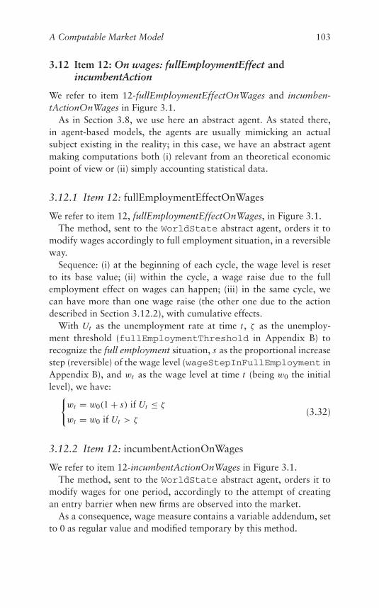
A Computable Market Model 103
3.12 Item 12: On wages: fullEmploymentEffect andincumbentAction
We refer to item 12-fullEmploymentEffectOnWages and incumben-tActionOnWages in Figure 3.1.
As in Section 3.8, we use here an abstract agent. As stated there,in agent-based models, the agents are usually mimicking an actualsubject existing in the reality; in this case, we have an abstract agentmaking computations both (i) relevant from an theoretical economicpoint of view or (ii) simply accounting statistical data.
3.12.1 Item 12: fullEmploymentEffectOnWages
We refer to item 12, fullEmploymentEffectOnWages, in Figure 3.1.The method, sent to the WorldState abstract agent, orders it to
modify wages accordingly to full employment situation, in a reversibleway.
Sequence: (i) at the beginning of each cycle, the wage level is resetto its base value; (ii) within the cycle, a wage raise due to the fullemployment effect on wages can happen; (iii) in the same cycle, wecan have more than one wage raise (the other one due to the actiondescribed in Section 3.12.2), with cumulative effects.
With Ut as the unemployment rate at time t , ζ as the unemploy-ment threshold (fullEmploymentThreshold in Appendix B) torecognize the full employment situation, s as the proportional increasestep (reversible) of the wage level (wageStepInFullEmployment inAppendix B), and wt as the wage level at time t (being w0 the initiallevel), we have:{
wt = w0(1 + s) if Ut ≤ ζ
wt = w0 if Ut > ζ(3.32)
3.12.2 Item 12: incumbentActionOnWages
We refer to item 12-incumbentActionOnWages in Figure 3.1.The method, sent to the WorldState abstract agent, orders it to
modify wages for one period, accordingly to the attempt of creatingan entry barrier when new firms are observed into the market.
As a consequence, wage measure contains a variable addendum, setto 0 as regular value and modified temporary by this method.
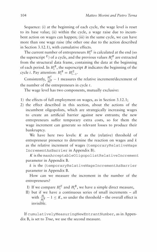
104 Matteo Morini and Pietro Terna
Sequence: (i) at the beginning of each cycle, the wage level is resetto its base value; (ii) within the cycle, a wage raise due to incum-bent action on wages can happen; (iii) in the same cycle, we can havemore than one wage raise (the other one due to the action describedin Section 3.12.1), with cumulative effects.
The current number of entrepreneurs H Et is calculated at the end (so
the superscript E ) of a cycle, and the previous values H Bi are extracted
from the structural data frame, containing the data at the beginningof each period. In H B
i , the superscript B indicates the beginning of thecycle i . Pay attention: H B
i = H Ei−1.
Consistently, H Et
H Bt
− 1 measures the relative increment/decrement of
the number of the entrepreneurs in cycle t .The wage level has two components, mutually exclusive:
1) the effects of full employment on wages, as in Section 3.12.1;2) the effect described in this section, about the actions of the
incumbent oligopolists, which are strategically increasing wagesto create an artificial barrier against new entrants; the newentrepreneurs suffer temporary extra costs, so for them thewage increment can generate so relevant losses to produce theirbankruptcy.
We have here two levels: K as the (relative) threshold ofentrepreneur presence to determine the reaction on wages and kas the relative increment of wages (temporaryRelativeWageIncrementAsBarrier in Appendix B).
K is the maxAcceptableOligopolistRelativeIncrementparameter in Appendix B.
k is the (temporaryRelativeWageIncrementAsBarrierparameter in Appendix B.
How can we measure the increment in the number of theentrepreneurs?
I) If we compare H Et and H B
t , we have a simple direct measure,II) but if we have a continuous series of small increments – all
with Ht
H Bt
− 1 ≤ K , so under the threshold – the overall effect is
invisible.
If cumulativelyMeasuringNewEntrantNumber, as in Appen-dix B, is set to True, we use the second measure.
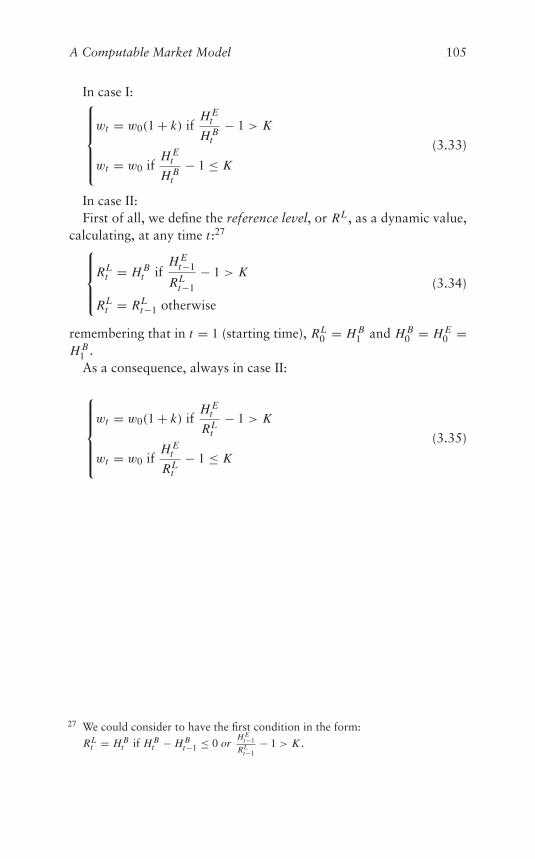
A Computable Market Model 105
In case I:⎧⎪⎪⎪⎪⎨⎪⎪⎪⎪⎩wt = w0(1 + k) if
H Et
H Bt
− 1 > K
wt = w0 ifH E
t
H Bt
− 1 ≤ K
(3.33)
In case II:First of all, we define the reference level, or RL , as a dynamic value,
calculating, at any time t :27⎧⎪⎪⎨⎪⎪⎩RL
t = H Bt if
H Et−1
RLt−1
− 1 > K
RLt = RL
t−1 otherwise
(3.34)
remembering that in t = 1 (starting time), RL0 = H B
1 and H B0 = H E
0 =H B
1 .As a consequence, always in case II:
⎧⎪⎪⎪⎪⎨⎪⎪⎪⎪⎩wt = w0(1 + k) if
H Et
RLt
− 1 > K
wt = w0 ifH E
t
RLt
− 1 ≤ K
(3.35)
27 We could consider to have the first condition in the form:RL
t = H Bt if H B
t − H Bt−1 ≤ 0 or
H Et−1
RLt−1
− 1 > K .
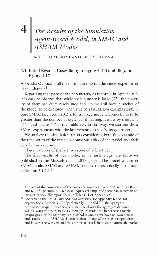
4 The Results of the SimulationAgent-Based Model, in SMAC andASHAM Modes
MATTEO MORINI AND PIETRO TERNA
4.1 Initial Results, Cases 0a (g in Figure 4.17) and 0b (h inFigure 4.17)
Appendix C contains all the information to run the model experimentsof this chapter.1
Regarding the space of the parameters, as reported in Appendix B,it is easy to observe that while their number is large (52), the major-ity of them are quite rarely modified. So we still have branches ofthe model to be explored. The value of startHayekianMarket, inpure SMAC (see Section 3.2.2 for a mixed mode reference), has to begreater than the number of cycle; so, if missing, it is set by default to“51” and not to “-” in the Table B.4. In this way, we can run thoseSMAC experiments with the last version of the oligopoly project.
We analyze the simulation results considering both the dynamic ofthe time series of the main economic variables of the model and theircorrelation structure.
These are cases of the last two rows of Table 4.25.The first results of our model, in its early stage, are those we
published in the Mazzoli et al. (2017) paper. The model was in itsSMAC mode. SMAC and ASHAM modes are technically introducedin Section 3.1.2.2 3
1 The sets of the parameters of the two experiments are reported in Tables B.3and B.4 of Appendix B. Each case requires the input of a few parameters in aninteractive way. We report them in Table C.1 of Appendix C.
2 Concerning the SMAC and ASHAM acrostics, see Appendix B and, forexplanations, Section 3.1.2. Synthetically, (i) in SMAC, the aggregateproduction in quantity at time t is compared with the aggregate demand invalue always at time t , to fix a clearing price under the hypothesis that theunique good of the economy is a perishable one, so we have no warehousesand stocks; (ii) in ASHAM, the interaction among sellers (the entrepreneurs)and buyers (the workers and the entrepreneurs) is built via an atomistic market
106
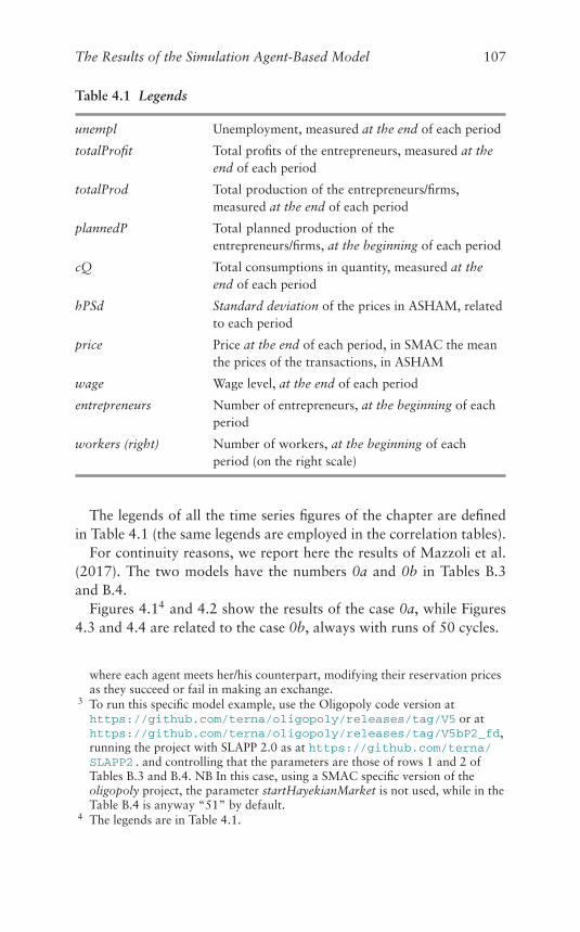
The Results of the Simulation Agent-Based Model 107
Table 4.1 Legends
unempl Unemployment, measured at the end of each period
totalProfit Total profits of the entrepreneurs, measured at theend of each period
totalProd Total production of the entrepreneurs/firms,measured at the end of each period
plannedP Total planned production of theentrepreneurs/firms, at the beginning of each period
cQ Total consumptions in quantity, measured at theend of each period
hPSd Standard deviation of the prices in ASHAM, relatedto each period
price Price at the end of each period, in SMAC the meanthe prices of the transactions, in ASHAM
wage Wage level, at the end of each period
entrepreneurs Number of entrepreneurs, at the beginning of eachperiod
workers (right) Number of workers, at the beginning of eachperiod (on the right scale)
The legends of all the time series figures of the chapter are definedin Table 4.1 (the same legends are employed in the correlation tables).
For continuity reasons, we report here the results of Mazzoli et al.(2017). The two models have the numbers 0a and 0b in Tables B.3and B.4.
Figures 4.14 and 4.2 show the results of the case 0a, while Figures4.3 and 4.4 are related to the case 0b, always with runs of 50 cycles.
where each agent meets her/his counterpart, modifying their reservation pricesas they succeed or fail in making an exchange.
3 To run this specific model example, use the Oligopoly code version athttps://github.com/terna/oligopoly/releases/tag/V5 or athttps://github.com/terna/oligopoly/releases/tag/V5bP2_fd,running the project with SLAPP 2.0 as at https://github.com/terna/SLAPP2 . and controlling that the parameters are those of rows 1 and 2 ofTables B.3 and B.4. NB In this case, using a SMAC specific version of theoligopoly project, the parameter startHayekianMarket is not used, while in theTable B.4 is anyway “51” by default.
4 The legends are in Table 4.1.
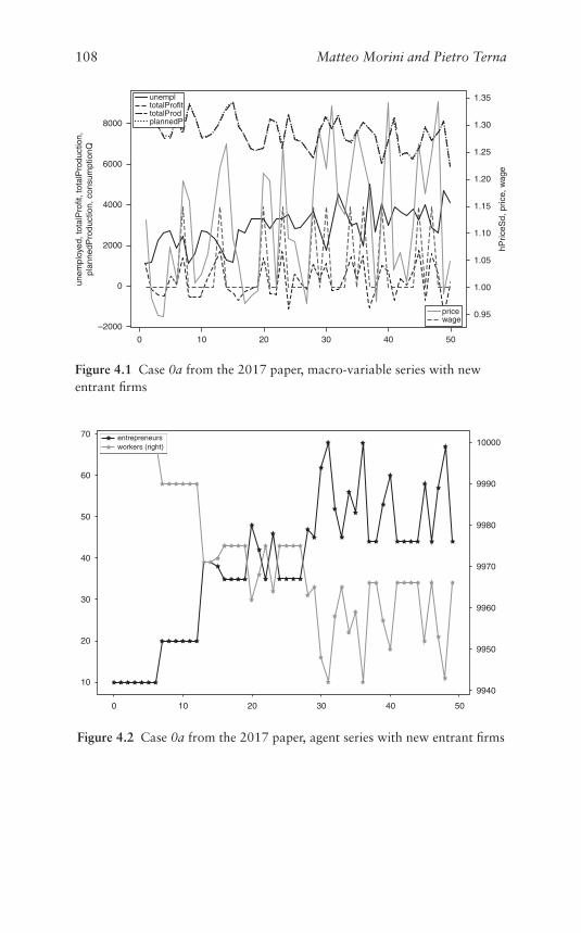
108 Matteo Morini and Pietro Terna
price
0 10 20 30 40 50
hPric
eSd,
pric
e, w
age
unem
ploy
ed, t
otal
Pro
fit, t
otal
Pro
duct
ion,
plan
nedP
rodu
ctio
n, c
onsu
mpt
ionQ
1.35
1.30
1.25
1.20
1.15
1.10
1.05
1.00
0.95
8000
6000
4000
2000
0
–2000wage
unempltotalProfittotalProdplannedP
Figure 4.1 Case 0a from the 2017 paper, macro-variable series with newentrant firms
0 10 20 30 40 50
9940
9950
9960
9970
9980
9990
10000
10
20
30
40
50
60
70 entrepreneursworkers (right)
Figure 4.2 Case 0a from the 2017 paper, agent series with new entrant firms
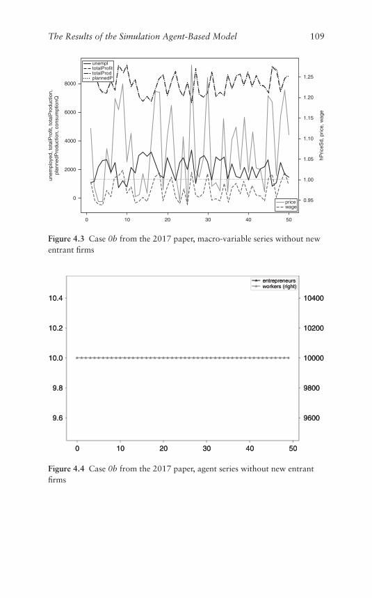
The Results of the Simulation Agent-Based Model 109
0 10 20 30 40 50
0.95
1.00
1.05
1.10
1.15
1.20
1.25
hPric
eSd,
pric
e, w
age
0
2000
4000
6000
8000
unem
ploy
ed, t
otal
Pro
fit, t
otal
Pro
duct
ion,
plan
nedP
rodu
ctio
n, c
onsu
mpt
ionQ
pricewage
unempltotalProfittotalProdplannedP
Figure 4.3 Case 0b from the 2017 paper, macro-variable series without newentrant firms
00 1010 2020 3030 4040 5050
96009600
98009800
1000010000
1020010200
1040010400
entrepreneursentrepreneursworkers (right)workers (right)
9.69.6
9.89.8
10.010.0
10.210.2
10.410.4
Figure 4.4 Case 0b from the 2017 paper, agent series without new entrantfirms
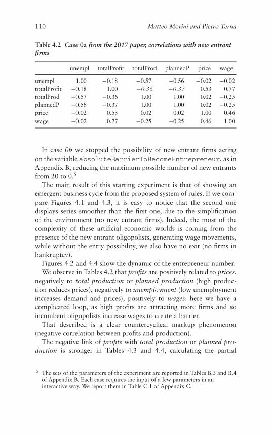
110 Matteo Morini and Pietro Terna
Table 4.2 Case 0a from the 2017 paper, correlations with new entrantfirms
unempl totalProfit totalProd plannedP price wage
unempl 1.00 −0.18 −0.57 −0.56 −0.02 −0.02totalProfit −0.18 1.00 −0.36 −0.37 0.53 0.77totalProd −0.57 −0.36 1.00 1.00 0.02 −0.25plannedP −0.56 −0.37 1.00 1.00 0.02 −0.25price −0.02 0.53 0.02 0.02 1.00 0.46wage −0.02 0.77 −0.25 −0.25 0.46 1.00
In case 0b we stopped the possibility of new entrant firms actingon the variable absoluteBarrierToBecomeEntrepreneur, as inAppendix B, reducing the maximum possible number of new entrantsfrom 20 to 0.5
The main result of this starting experiment is that of showing anemergent business cycle from the proposed system of rules. If we com-pare Figures 4.1 and 4.3, it is easy to notice that the second onedisplays series smoother than the first one, due to the simplificationof the environment (no new entrant firms). Indeed, the most of thecomplexity of these artificial economic worlds is coming from thepresence of the new entrant oligopolists, generating wage movements,while without the entry possibility, we also have no exit (no firms inbankruptcy).
Figures 4.2 and 4.4 show the dynamic of the entrepreneur number.We observe in Tables 4.2 that profits are positively related to prices,
negatively to total production or planned production (high produc-tion reduces prices), negatively to unemployment (low unemploymentincreases demand and prices), positively to wages: here we have acomplicated loop, as high profits are attracting more firms and soincumbent oligopolists increase wages to create a barrier.
That described is a clear countercyclical markup phenomenon(negative correlation between profits and production).
The negative link of profits with total production or planned pro-duction is stronger in Tables 4.3 and 4.4, calculating the partial
5 The sets of the parameters of the experiment are reported in Tables B.3 and B.4of Appendix B. Each case requires the input of a few parameters in aninteractive way. We report them in Table C.1 of Appendix C.
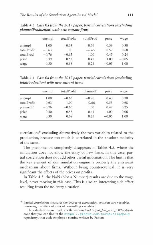
The Results of the Simulation Agent-Based Model 111
Table 4.3 Case 0a from the 2017 paper, partial correlations (excludingplannedProduction) with new entrant firms
unempl totalProfit totalProd price wage
unempl 1.00 −0.63 −0.76 0.39 0.30totalProfit −0.63 1.00 −0.65 0.52 0.68totalProd −0.76 −0.65 1.00 0.45 0.24price 0.39 0.52 0.45 1.00 −0.05wage 0.30 0.68 0.24 −0.05 1.00
Table 4.4 Case 0a from the 2017 paper, partial correlations (excludingtotalProduction) with new entrant firms
unempl totalProfit plannedP price wage
unempl 1.00 −0.63 −0.76 0.40 0.30totalProfit −0.63 1.00 −0.66 0.53 0.68plannedP −0.76 −0.66 1.00 0.47 0.25price 0.40 0.53 0.47 1.00 −0.06wage 0.30 0.68 0.25 −0.06 1.00
correlations6 excluding alternatively the two variables related to theproduction, because too much is correlated in the absolute majorityof the cases.
The phenomenon completely disappears in Tables 4.5, where thesimulation does not allow the entry of new firms. In this case, par-tial correlation does not add other useful information. The hint is thatthe key element of our simulation engine is properly the entry/exitmechanism about firms. Without being countercyclical, it is verysignificant the effects of the prices on profits.
In Table 4.5, the NaN (Not a Number) results are due to the wagelevel, never moving in this case. This is also an interesting side effectresulting from the no-entry situation.
6 Partial correlation measures the degree of association between two variables,removing the effect of a set of controlling variables.
The calculations are made via the readingCsvOutput_par_corr_BWter.ipynbcode that you can find in the https://github.com/terna/oligopolyrepository; that code employs a routine written by Fabian
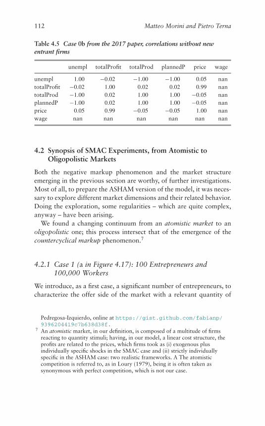
112 Matteo Morini and Pietro Terna
Table 4.5 Case 0b from the 2017 paper, correlations without newentrant firms
unempl totalProfit totalProd plannedP price wage
unempl 1.00 −0.02 −1.00 −1.00 0.05 nantotalProfit −0.02 1.00 0.02 0.02 0.99 nantotalProd −1.00 0.02 1.00 1.00 −0.05 nanplannedP −1.00 0.02 1.00 1.00 −0.05 nanprice 0.05 0.99 −0.05 −0.05 1.00 nanwage nan nan nan nan nan nan
4.2 Synopsis of SMAC Experiments, from Atomistic toOligopolistic Markets
Both the negative markup phenomenon and the market structureemerging in the previous section are worthy, of further investigations.Most of all, to prepare the ASHAM version of the model, it was neces-sary to explore different market dimensions and their related behavior.Doing the exploration, some regularities – which are quite complex,anyway – have been arising.
We found a changing continuum from an atomistic market to anoligopolistic one; this process intersect that of the emergence of thecountercyclical markup phenomenon.7
4.2.1 Case 1 (a in Figure 4.17): 100 Entrepreneurs and100,000 Workers
We introduce, as a first case, a significant number of entrepreneurs, tocharacterize the offer side of the market with a relevant quantity of
Pedregosa-Izquierdo, online at https://gist.github.com/fabianp/9396204419c7b638d38f .
7 An atomistic market, in our definition, is composed of a multitude of firmsreacting to quantity stimuli; having, in our model, a linear cost structure, theprofits are related to the prices, which firms took as (i) exogenous plusindividually specific shocks in the SMAC case and (ii) strictly individuallyspecific in the ASHAM case: two realistic frameworks. A The atomisticcompetition is referred to, as in Loury (1979), being it is often taken assynonymous with perfect competition, which is not our case.
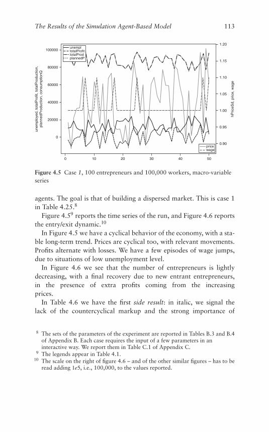
The Results of the Simulation Agent-Based Model 113
pricewage
unempltotalProfittotalProdplannedP
unem
ploy
ed, t
otal
Pro
fit, t
otal
Pro
duct
ion,
plan
nedP
rodu
ctio
n, c
onsu
mpt
ionQ
0 10 20 30 40 50
0.90
0.95
1.00
1.05
1.10
1.15
1.20
hPric
eSd,
pric
e, w
age
0
20000
40000
60000
80000
100000
Figure 4.5 Case 1, 100 entrepreneurs and 100,000 workers, macro-variableseries
agents. The goal is that of building a dispersed market. This is case 1in Table 4.25.8
Figure 4.59 reports the time series of the run, and Figure 4.6 reportsthe entry/exit dynamic.10
In Figure 4.5 we have a cyclical behavior of the economy, with a sta-ble long-term trend. Prices are cyclical too, with relevant movements.Profits alternate with losses. We have a few episodes of wage jumps,due to situations of low unemployment level.
In Figure 4.6 we see that the number of entrepreneurs is lightlydecreasing, with a final recovery due to new entrant entrepreneurs,in the presence of extra profits coming from the increasingprices.
In Table 4.6 we have the first side result: in italic, we signal thelack of the countercyclical markup and the strong importance of
8 The sets of the parameters of the experiment are reported in Tables B.3 and B.4of Appendix B. Each case requires the input of a few parameters in aninteractive way. We report them in Table C.1 of Appendix C.
9 The legends appear in Table 4.1.10 The scale on the right of figure 4.6 – and of the other similar figures – has to be
read adding 1e5, i.e., 100,000, to the values reported.
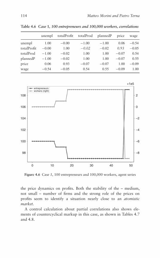
114 Matteo Morini and Pietro Terna
Table 4.6 Case 1, 100 entrepreneurs and 100,000 workers, correlations
unempl totalProfit totalProd plannedP price wage
unempl 1.00 −0.00 −1.00 −1.00 0.06 −0.54
totalProfit −0.00 1.00 −0.02 −0.02 0.93 −0.05
totalProd −1.00 −0.02 1.00 1.00 −0.07 0.54
plannedP −1.00 −0.02 1.00 1.00 −0.07 0.55
price 0.06 0.93 −0.07 −0.07 1.00 −0.09
wage −0.54 −0.05 0.54 0.55 −0.09 1.00
entrepreneursworkers (right)
108
106
104
102
100
98
0 10 20 30 40 50
–8
–6
–4
–2
0
2
+1e5
Figure 4.6 Case 1, 100 entrepreneurs and 100,000 workers, agent series
the price dynamics on profits. Both the stability of the – medium,not small – number of firms and the strong role of the prices onprofits seem to identify a situation nearly close to an atomisticmarket.
A control calculation about partial correlations also shows ele-ments of countercyclical markup in this case, as shown in Tables 4.7and 4.8.
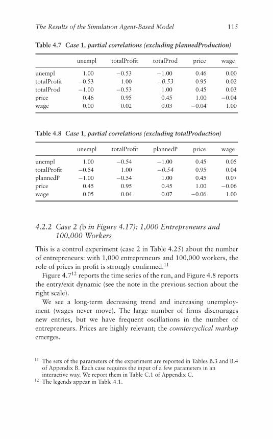
The Results of the Simulation Agent-Based Model 115
Table 4.7 Case 1, partial correlations (excluding plannedProduction)
unempl totalProfit totalProd price wage
unempl 1.00 −0.53 −1.00 0.46 0.00totalProfit −0.53 1.00 −0.53 0.95 0.02totalProd −1.00 −0.53 1.00 0.45 0.03price 0.46 0.95 0.45 1.00 −0.04wage 0.00 0.02 0.03 −0.04 1.00
Table 4.8 Case 1, partial correlations (excluding totalProduction)
unempl totalProfit plannedP price wage
unempl 1.00 −0.54 −1.00 0.45 0.05totalProfit −0.54 1.00 −0.54 0.95 0.04plannedP −1.00 −0.54 1.00 0.45 0.07price 0.45 0.95 0.45 1.00 −0.06wage 0.05 0.04 0.07 −0.06 1.00
4.2.2 Case 2 (b in Figure 4.17): 1,000 Entrepreneurs and100,000 Workers
This is a control experiment (case 2 in Table 4.25) about the numberof entrepreneurs: with 1,000 entrepreneurs and 100,000 workers, therole of prices in profit is strongly confirmed.11
Figure 4.712 reports the time series of the run, and Figure 4.8 reportsthe entry/exit dynamic (see the note in the previous section about theright scale).
We see a long-term decreasing trend and increasing unemploy-ment (wages never move). The large number of firms discouragesnew entries, but we have frequent oscillations in the number ofentrepreneurs. Prices are highly relevant; the countercyclical markupemerges.
11 The sets of the parameters of the experiment are reported in Tables B.3 and B.4of Appendix B. Each case requires the input of a few parameters in aninteractive way. We report them in Table C.1 of Appendix C.
12 The legends appear in Table 4.1.
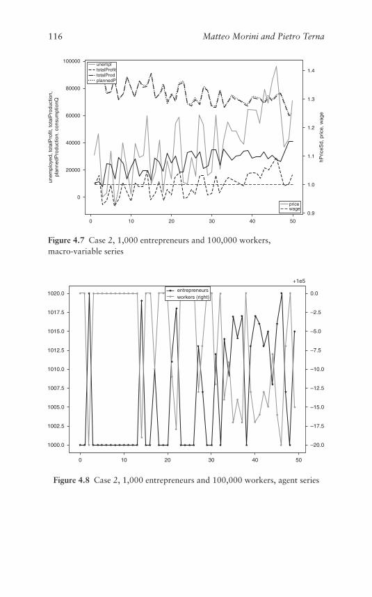
116 Matteo Morini and Pietro Ternaun
empl
oyed
, tot
alP
rofit
, tot
alP
rodu
ctio
n,pl
anne
dPro
duct
ion.
con
sum
ptio
nQ
0 10 20 30 40 50
0.9
1.0
1.1
1.2
1.3
1.4
hPric
eSd,
pric
e, w
age
0
20000
40000
60000
80000
100000
pricewage
unempltotalProfittotalProdplannedP
Figure 4.7 Case 2, 1,000 entrepreneurs and 100,000 workers,macro-variable series
0 10 20 30 40 50
–20.0
–17.5
–15.0
–12.5
–10.0
–7.5
–5.0
–2.5
0.0
+1e5
1000.0
1002.5
1005.0
1007.5
1010.0
1012.5
1015.0
1017.5
1020.0entrepreneursworkers (right)
Figure 4.8 Case 2, 1,000 entrepreneurs and 100,000 workers, agent series
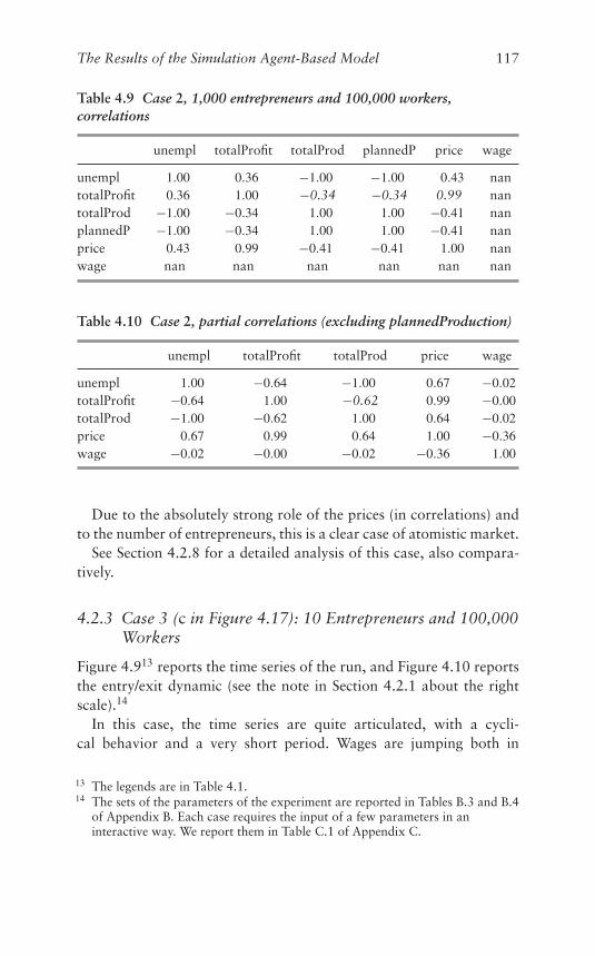
The Results of the Simulation Agent-Based Model 117
Table 4.9 Case 2, 1,000 entrepreneurs and 100,000 workers,correlations
unempl totalProfit totalProd plannedP price wage
unempl 1.00 0.36 −1.00 −1.00 0.43 nantotalProfit 0.36 1.00 −0.34 −0.34 0.99 nantotalProd −1.00 −0.34 1.00 1.00 −0.41 nanplannedP −1.00 −0.34 1.00 1.00 −0.41 nanprice 0.43 0.99 −0.41 −0.41 1.00 nanwage nan nan nan nan nan nan
Table 4.10 Case 2, partial correlations (excluding plannedProduction)
unempl totalProfit totalProd price wage
unempl 1.00 −0.64 −1.00 0.67 −0.02totalProfit −0.64 1.00 −0.62 0.99 −0.00totalProd −1.00 −0.62 1.00 0.64 −0.02price 0.67 0.99 0.64 1.00 −0.36wage −0.02 −0.00 −0.02 −0.36 1.00
Due to the absolutely strong role of the prices (in correlations) andto the number of entrepreneurs, this is a clear case of atomistic market.
See Section 4.2.8 for a detailed analysis of this case, also compara-tively.
4.2.3 Case 3 (c in Figure 4.17): 10 Entrepreneurs and 100,000Workers
Figure 4.913 reports the time series of the run, and Figure 4.10 reportsthe entry/exit dynamic (see the note in Section 4.2.1 about the rightscale).14
In this case, the time series are quite articulated, with a cycli-cal behavior and a very short period. Wages are jumping both in
13 The legends are in Table 4.1.14 The sets of the parameters of the experiment are reported in Tables B.3 and B.4
of Appendix B. Each case requires the input of a few parameters in aninteractive way. We report them in Table C.1 of Appendix C.
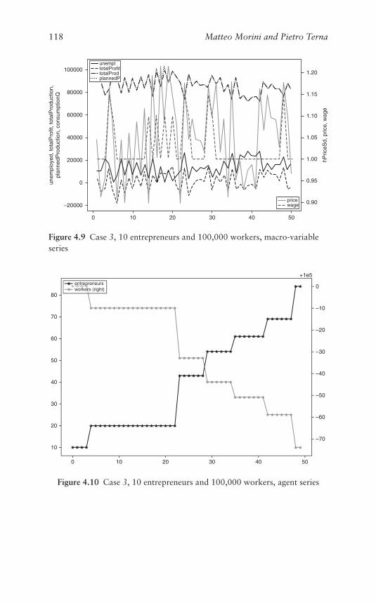
118 Matteo Morini and Pietro Terna
pricewage
unempltotalProfittotalProdplannedP
100000
80000
60000
40000
unem
ploy
ed, t
otal
Pro
fit, t
otal
Pro
duct
ion,
plan
nedP
rodu
ctio
n, c
onsu
mpt
ionQ
20000
0
0 10 30
0.90
0.95
1.00
1.10
hPric
eSd,
pric
e, w
age
1.20
1.15
1.05
504020
–20000
Figure 4.9 Case 3, 10 entrepreneurs and 100,000 workers, macro-variableseries
entrepreneursworkers (right)
80
70
60
50
40
30
20
10
0 10 20 30 40 50
0
+1e5
–10
–20
–30
–40
–50
–60
–70
Figure 4.10 Case 3, 10 entrepreneurs and 100,000 workers, agent series
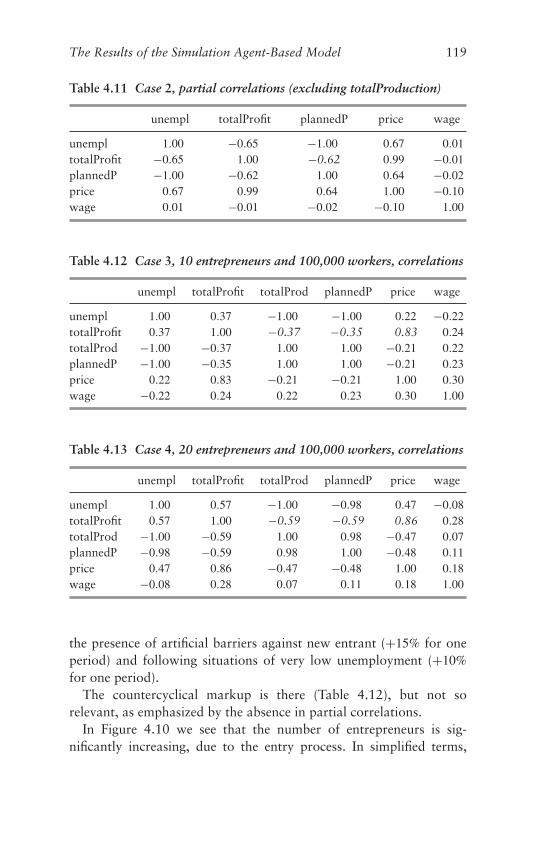
The Results of the Simulation Agent-Based Model 119
Table 4.11 Case 2, partial correlations (excluding totalProduction)
unempl totalProfit plannedP price wage
unempl 1.00 −0.65 −1.00 0.67 0.01totalProfit −0.65 1.00 −0.62 0.99 −0.01plannedP −1.00 −0.62 1.00 0.64 −0.02price 0.67 0.99 0.64 1.00 −0.10wage 0.01 −0.01 −0.02 −0.10 1.00
Table 4.12 Case 3, 10 entrepreneurs and 100,000 workers, correlations
unempl totalProfit totalProd plannedP price wage
unempl 1.00 0.37 −1.00 −1.00 0.22 −0.22totalProfit 0.37 1.00 −0.37 −0.35 0.83 0.24totalProd −1.00 −0.37 1.00 1.00 −0.21 0.22plannedP −1.00 −0.35 1.00 1.00 −0.21 0.23price 0.22 0.83 −0.21 −0.21 1.00 0.30wage −0.22 0.24 0.22 0.23 0.30 1.00
Table 4.13 Case 4, 20 entrepreneurs and 100,000 workers, correlations
unempl totalProfit totalProd plannedP price wage
unempl 1.00 0.57 −1.00 −0.98 0.47 −0.08totalProfit 0.57 1.00 −0.59 −0.59 0.86 0.28totalProd −1.00 −0.59 1.00 0.98 −0.47 0.07plannedP −0.98 −0.59 0.98 1.00 −0.48 0.11price 0.47 0.86 −0.47 −0.48 1.00 0.18wage −0.08 0.28 0.07 0.11 0.18 1.00
the presence of artificial barriers against new entrant (+15% for oneperiod) and following situations of very low unemployment (+10%for one period).
The countercyclical markup is there (Table 4.12), but not sorelevant, as emphasized by the absence in partial correlations.
In Figure 4.10 we see that the number of entrepreneurs is sig-nificantly increasing, due to the entry process. In simplified terms,
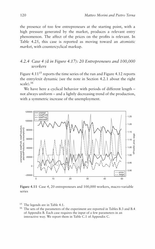
120 Matteo Morini and Pietro Terna
the presence of too few entrepreneurs at the starting point, with ahigh pressure generated by the market, produces a relevant entryphenomenon. The affect of the prices on the profits is relevant. InTable 4.25, this case is reported as moving toward an atomisticmarket, with countercyclical markup.
4.2.4 Case 4 (d in Figure 4.17): 20 Entrepreneurs and 100,000workers
Figure 4.1115 reports the time series of the run and Figure 4.12 reportsthe entry/exit dynamic (see the note in Section 4.2.1 about the rightscale).16
We have here a cyclical behavior with periods of different length –not always uniform – and a lightly decreasing trend of the production,with a symmetric increase of the unemployment.
0 10 20 30 40 50
hPric
eSd,
pric
e, w
age
unem
ploy
ed, t
otal
Pro
fit, t
otal
Pro
duct
ion,
plan
nedP
rodu
ctio
n, c
onsu
mpt
ionQ
1.25
1.20
1.15
1.10
1.05
1.00
0.95
0.90
100000
80000
120000
60000
40000
20000
0
–20000
unempltotalProfittotalProdplannedP
pricewage
Figure 4.11 Case 4, 20 entrepreneurs and 100,000 workers, macro-variableseries
15 The legends are in Table 4.1.16 The sets of the parameters of the experiment are reported in Tables B.3 and B.4
of Appendix B. Each case requires the input of a few parameters in aninteractive way. We report them in Table C.1 of Appendix C.
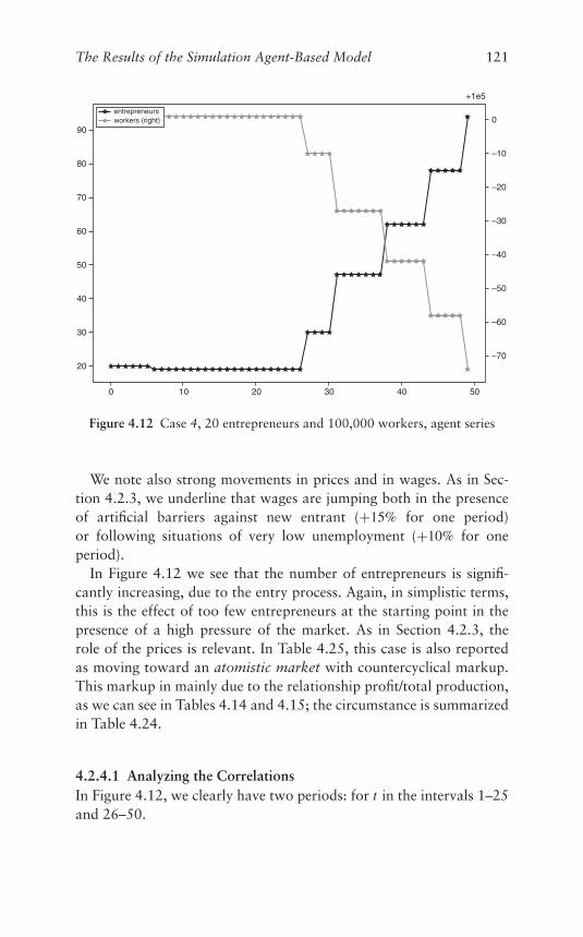
The Results of the Simulation Agent-Based Model 121
entrepreneursworkers (right)
500 10 20 30 40
0
+1e5
–10
–20
–30
–40
–50
–60
–70
90
80
70
60
50
40
30
20
Figure 4.12 Case 4, 20 entrepreneurs and 100,000 workers, agent series
We note also strong movements in prices and in wages. As in Sec-tion 4.2.3, we underline that wages are jumping both in the presenceof artificial barriers against new entrant (+15% for one period)or following situations of very low unemployment (+10% for oneperiod).
In Figure 4.12 we see that the number of entrepreneurs is signifi-cantly increasing, due to the entry process. Again, in simplistic terms,this is the effect of too few entrepreneurs at the starting point in thepresence of a high pressure of the market. As in Section 4.2.3, therole of the prices is relevant. In Table 4.25, this case is also reportedas moving toward an atomistic market with countercyclical markup.This markup in mainly due to the relationship profit/total production,as we can see in Tables 4.14 and 4.15; the circumstance is summarizedin Table 4.24.
4.2.4.1 Analyzing the CorrelationsIn Figure 4.12, we clearly have two periods: for t in the intervals 1–25and 26–50.
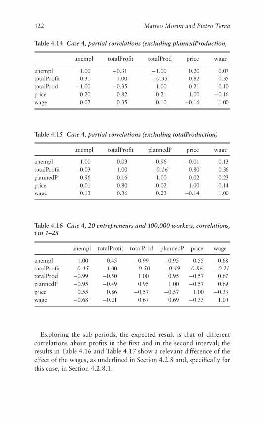
122 Matteo Morini and Pietro Terna
Table 4.14 Case 4, partial correlations (excluding plannedProduction)
unempl totalProfit totalProd price wage
unempl 1.00 −0.31 −1.00 0.20 0.07totalProfit −0.31 1.00 −0.35 0.82 0.35totalProd −1.00 −0.35 1.00 0.21 0.10price 0.20 0.82 0.21 1.00 −0.16wage 0.07 0.35 0.10 −0.16 1.00
Table 4.15 Case 4, partial correlations (excluding totalProduction)
unempl totalProfit plannedP price wage
unempl 1.00 −0.03 −0.96 −0.01 0.13totalProfit −0.03 1.00 −0.16 0.80 0.36plannedP −0.96 −0.16 1.00 0.02 0.23price −0.01 0.80 0.02 1.00 −0.14wage 0.13 0.36 0.23 −0.14 1.00
Table 4.16 Case 4, 20 entrepreneurs and 100,000 workers, correlations,t in 1–25
unempl totalProfit totalProd plannedP price wage
unempl 1.00 0.45 −0.99 −0.95 0.55 −0.68totalProfit 0.45 1.00 −0.50 −0.49 0.86 −0.21totalProd −0.99 −0.50 1.00 0.95 −0.57 0.67plannedP −0.95 −0.49 0.95 1.00 −0.57 0.69price 0.55 0.86 −0.57 −0.57 1.00 −0.33wage −0.68 −0.21 0.67 0.69 −0.33 1.00
Exploring the sub-periods, the expected result is that of differentcorrelations about profits in the first and in the second interval; theresults in Table 4.16 and Table 4.17 show a relevant difference of theeffect of the wages, as underlined in Section 4.2.8 and, specifically forthis case, in Section 4.2.8.1.
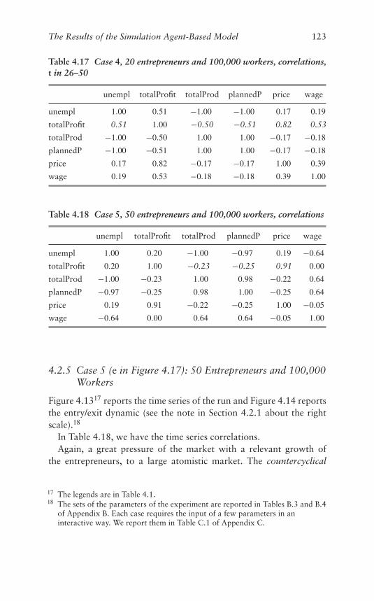
The Results of the Simulation Agent-Based Model 123
Table 4.17 Case 4, 20 entrepreneurs and 100,000 workers, correlations,t in 26–50
unempl totalProfit totalProd plannedP price wage
unempl 1.00 0.51 −1.00 −1.00 0.17 0.19
totalProfit 0.51 1.00 −0.50 −0.51 0.82 0.53
totalProd −1.00 −0.50 1.00 1.00 −0.17 −0.18
plannedP −1.00 −0.51 1.00 1.00 −0.17 −0.18
price 0.17 0.82 −0.17 −0.17 1.00 0.39
wage 0.19 0.53 −0.18 −0.18 0.39 1.00
Table 4.18 Case 5, 50 entrepreneurs and 100,000 workers, correlations
unempl totalProfit totalProd plannedP price wage
unempl 1.00 0.20 −1.00 −0.97 0.19 −0.64
totalProfit 0.20 1.00 −0.23 −0.25 0.91 0.00
totalProd −1.00 −0.23 1.00 0.98 −0.22 0.64
plannedP −0.97 −0.25 0.98 1.00 −0.25 0.64
price 0.19 0.91 −0.22 −0.25 1.00 −0.05
wage −0.64 0.00 0.64 0.64 −0.05 1.00
4.2.5 Case 5 (e in Figure 4.17): 50 Entrepreneurs and 100,000Workers
Figure 4.1317 reports the time series of the run and Figure 4.14 reportsthe entry/exit dynamic (see the note in Section 4.2.1 about the rightscale).18
In Table 4.18, we have the time series correlations.Again, a great pressure of the market with a relevant growth of
the entrepreneurs, to a large atomistic market. The countercyclical
17 The legends are in Table 4.1.18 The sets of the parameters of the experiment are reported in Tables B.3 and B.4
of Appendix B. Each case requires the input of a few parameters in aninteractive way. We report them in Table C.1 of Appendix C.
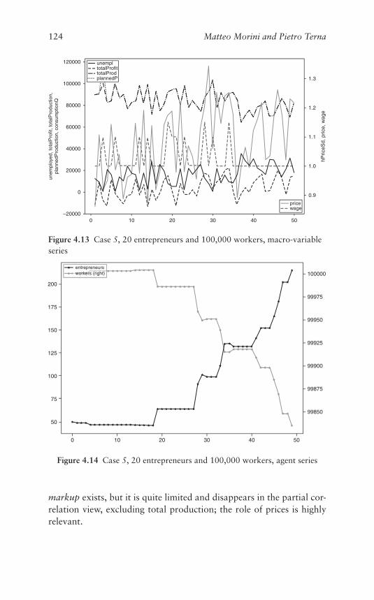
124 Matteo Morini and Pietro Terna
pricewage
120000
100000
80000
60000
40000
20000
0
0–20000
10 20 30 5040
0.9
1.0
1.1
1.2
1.3
hPric
eSd,
pric
e, w
age
unem
ploy
ed, t
otal
Pro
fit, t
otal
Pro
duct
ion,
plan
nedP
rodu
ctio
n, c
onsu
mpt
ionQ
unempltotalProfittotalProdplannedP
Figure 4.13 Case 5, 20 entrepreneurs and 100,000 workers, macro-variableseries
150
100
125
75
50
10 20 30 40 500
175
200
99850
99875
99925
99950
99975
100000
99900
entrepreneursworkers (right)
Figure 4.14 Case 5, 20 entrepreneurs and 100,000 workers, agent series
markup exists, but it is quite limited and disappears in the partial cor-relation view, excluding total production; the role of prices is highlyrelevant.
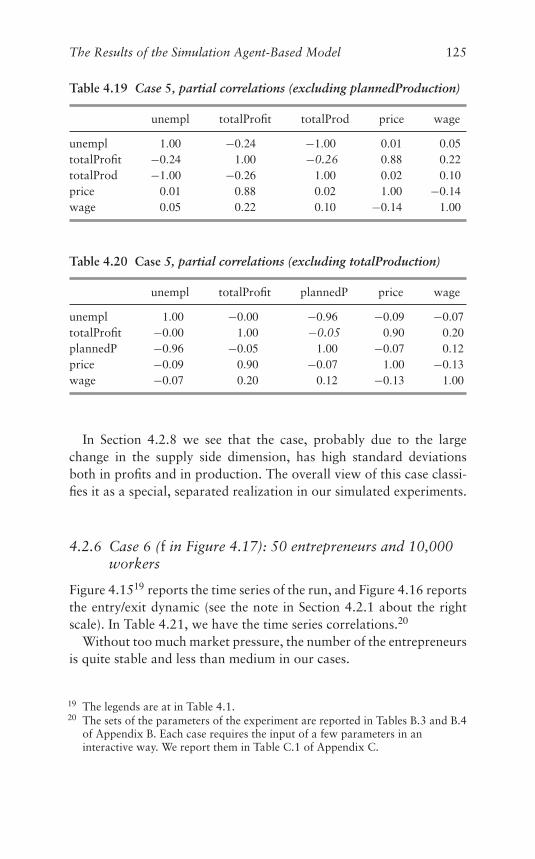
The Results of the Simulation Agent-Based Model 125
Table 4.19 Case 5, partial correlations (excluding plannedProduction)
unempl totalProfit totalProd price wage
unempl 1.00 −0.24 −1.00 0.01 0.05totalProfit −0.24 1.00 −0.26 0.88 0.22totalProd −1.00 −0.26 1.00 0.02 0.10price 0.01 0.88 0.02 1.00 −0.14wage 0.05 0.22 0.10 −0.14 1.00
Table 4.20 Case 5, partial correlations (excluding totalProduction)
unempl totalProfit plannedP price wage
unempl 1.00 −0.00 −0.96 −0.09 −0.07totalProfit −0.00 1.00 −0.05 0.90 0.20plannedP −0.96 −0.05 1.00 −0.07 0.12price −0.09 0.90 −0.07 1.00 −0.13wage −0.07 0.20 0.12 −0.13 1.00
In Section 4.2.8 we see that the case, probably due to the largechange in the supply side dimension, has high standard deviationsboth in profits and in production. The overall view of this case classi-fies it as a special, separated realization in our simulated experiments.
4.2.6 Case 6 (f in Figure 4.17): 50 entrepreneurs and 10,000workers
Figure 4.1519 reports the time series of the run, and Figure 4.16 reportsthe entry/exit dynamic (see the note in Section 4.2.1 about the rightscale). In Table 4.21, we have the time series correlations.20
Without too much market pressure, the number of the entrepreneursis quite stable and less than medium in our cases.
19 The legends are at in Table 4.1.20 The sets of the parameters of the experiment are reported in Tables B.3 and B.4
of Appendix B. Each case requires the input of a few parameters in aninteractive way. We report them in Table C.1 of Appendix C.
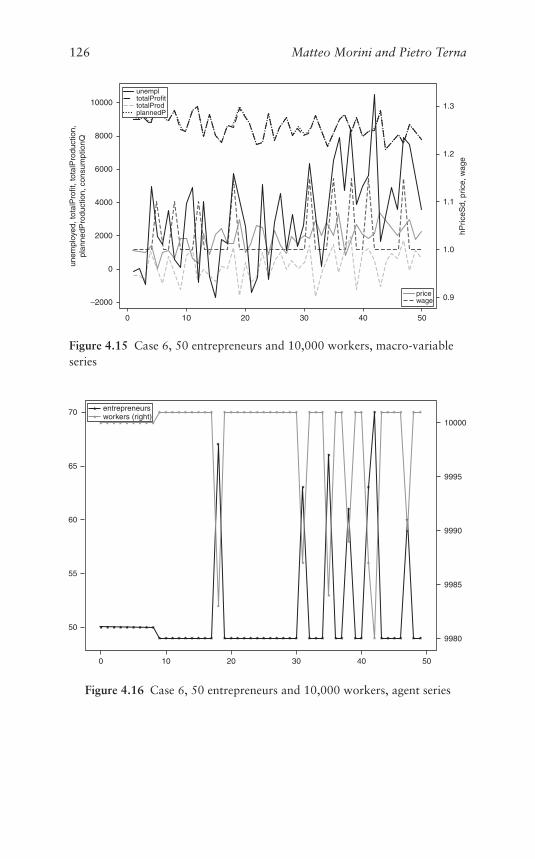
126 Matteo Morini and Pietro Ternaun
empl
oyed
, tot
alP
rofit
, tot
alP
rodu
ctio
n,pl
anne
dPro
duct
ion,
con
sum
ptio
nQ
10000
8000
6000
4000
2000
0
–2000
0 10 20 30 40 50
0.9
1.0
1.1
1.2
hPric
eSd,
pric
e, w
age
1.3
pricewage
unempltotalProfittotalProdplannedP
Figure 4.15 Case 6, 50 entrepreneurs and 10,000 workers, macro-variableseries
70
65
60
55
50
0 10 20 30 40 50
9980
9985
9990
9995
10000
entrepreneursworkers (right)
Figure 4.16 Case 6, 50 entrepreneurs and 10,000 workers, agent series

The Results of the Simulation Agent-Based Model 127
Table 4.21 Case 6, 50 entrepreneurs and 10,000 workers, correlations
unempl totalProfit totalProd plannedP price wage
unempl 1.00 −0.09 −0.53 −0.54 0.38 −0.17totalProfit −0.09 1.00 −0.44 −0.42 0.65 0.46totalProd −0.53 −0.44 1.00 1.00 −0.25 0.01plannedP −0.54 −0.42 1.00 1.00 −0.24 0.03price 0.38 0.65 −0.25 −0.24 1.00 0.34wage −0.17 0.46 0.01 0.03 0.34 1.00
Table 4.22 Case 6, partial correlations (excluding plannedProduction)
unempl totalProfit totalProd price wage
unempl 1.00 −0.80 −0.81 0.80 −0.00totalProfit −0.80 1.00 −0.80 0.84 0.24totalProd −0.81 −0.80 1.00 0.66 0.15price 0.80 0.84 0.66 1.00 0.03wage −0.00 0.24 0.15 0.03 1.00
See Section 4.24 for a detailed analysis of this case (also com-paratively), but immediately we can note the presence of thecountercyclical markup in Table 4.21 and an even stronger presencein Tables 4.22 and 4.23.
4.2.7 Summarizing Countercyclical Markup Presence in Cases0a to 6
Table 4.24 summarizes the countercyclical markup presence in thedifferent cases.
4.2.8 Synopsis of Cases from 0a to 6, in the SMAC Economy
Table 4.25 resumes our focus on of (i) the size of the market as num-ber of entrepreneurs, (ii) the entry/exit phenomenon, (iii) the prices,(iv) the dynamic of the unemployment, and (v) the wage level, onthe types of the emerging markets and on the countercyclical markup(if any).
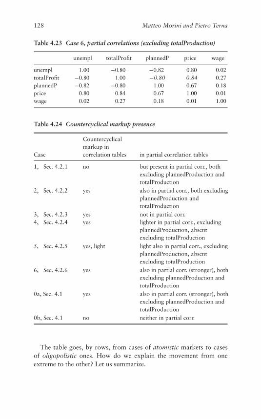
128 Matteo Morini and Pietro Terna
Table 4.23 Case 6, partial correlations (excluding totalProduction)
unempl totalProfit plannedP price wage
unempl 1.00 −0.80 −0.82 0.80 0.02totalProfit −0.80 1.00 −0.80 0.84 0.27plannedP −0.82 −0.80 1.00 0.67 0.18price 0.80 0.84 0.67 1.00 0.01wage 0.02 0.27 0.18 0.01 1.00
Table 4.24 Countercyclical markup presence
Countercyclicalmarkup in
Case correlation tables in partial correlation tables
1, Sec. 4.2.1 no but present in partial corr., bothexcluding plannedProduction andtotalProduction
2, Sec. 4.2.2 yes also in partial corr., both excludingplannedProduction andtotalProduction
3, Sec. 4.2.3 yes not in partial corr.4, Sec. 4.2.4 yes lighter in partial corr., excluding
plannedProduction, absentexcluding totalProduction
5, Sec. 4.2.5 yes, light light also in partial corr., excludingplannedProduction, absentexcluding totalProduction
6, Sec. 4.2.6 yes also in partial corr. (stronger), bothexcluding plannedProduction andtotalProduction
0a, Sec. 4.1 yes also in partial corr. (stronger), bothexcluding plannedProduction andtotalProduction
0b, Sec. 4.1 no neither in partial corr.
The table goes, by rows, from cases of atomistic markets to casesof oligopolistic ones. How do we explain the movement from oneextreme to the other? Let us summarize.
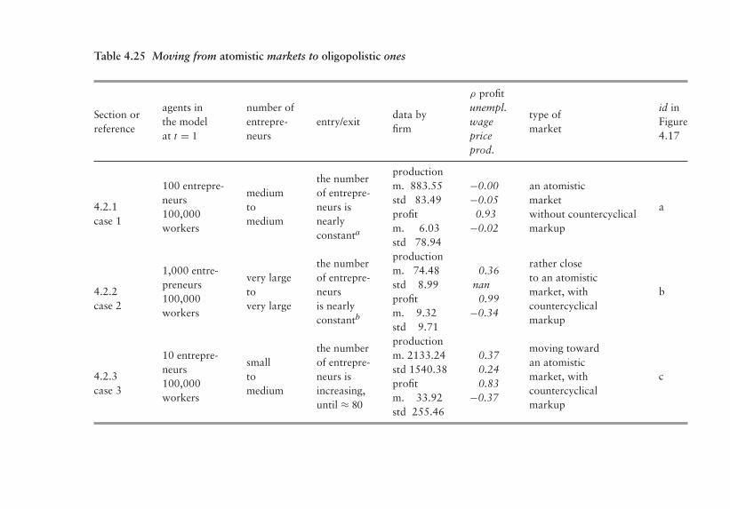
Table 4.25 Moving from atomistic markets to oligopolistic ones
Section orreference
agents inthe modelat t = 1
number ofentrepre-neurs
entry/exitdata byfirm
ρ profitunempl.wagepriceprod.
type ofmarket
id inFigure4.17
4.2.1case 1
100 entrepre-neurs100,000workers
mediumtomedium
the numberof entrepre-neurs isnearlyconstanta
productionm. 883.55std 83.49profitm. 6.03std 78.94
−0.00−0.05
0.93−0.02
an atomisticmarketwithout countercyclicalmarkup
a
4.2.2case 2
1,000 entre-preneurs100,000workers
very largetovery large
the numberof entrepre-neursis nearlyconstantb
productionm. 74.48std 8.99profitm. 9.32std 9.71
0.36nan
0.99−0.34
rather closeto an atomisticmarket, withcountercyclicalmarkup
b
4.2.3case 3
10 entrepre-neurs100,000workers
smalltomedium
the numberof entrepre-neurs isincreasing,until ≈ 80
productionm. 2133.24std 1540.38profitm. 33.92std 255.46
0.370.240.83
−0.37
moving towardan atomisticmarket, withcountercyclicalmarkup
c
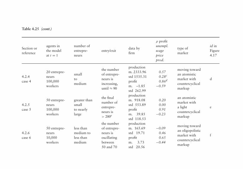
Table 4.25 (cont.)
Section orreference
agents inthe modelat t = 1
number ofentrepre-neurs
entry/exitdata byfirm
ρ profitunempl.wagepriceprod.
type ofmarket
id inFigure4.17
4.2.4case 4
20 entrepre-neurs100,000workers
smalltomedium
the numberof entrepre-neurs isincreasing,until ≈ 90
productionm. 2333.96std 1535.31profitm. –1.85std 262.99
0.570.28c
0.86d
−0.59
moving towardan atomisticmarket withcountercyclicalmarkup
d
4.2.5case 5
50 entrepre-neurs100,000workers
greater thansmallto nearlylarge
the finalnumber ofentrepre-neurs is> 200e
productionm. 918.08std 553.89profitm. 39.85std 118.53
0.200.000.91
−0.23
an atomisticmarket witha lightcountercyclicalmarkup
e
4.2.6case 6
50 entrepre-neurs10,000workers
less thanmedium toless thanmedium
the numberof entrepre-neurs isoscillatingbetween50 and 70
productionm. 165.69std 19.71profitm. 3.73std 20.56
−0.090.460.65
−0.44
moving towardan oligopolisticmarket withcountercyclicalmarkup
f
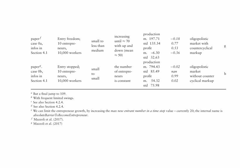
paper f
case 0a,infos inSection 4.1
Entry freedom;10 entrepre-neurs,10,000 workers
small toless thanmedium
increasinguntil ≈ 70with up anddown (mean≈ 50)
productionm. 197.71std 135.34profitm. –6.30std 32.63
−0.180.770.53−0.36
oligopolisticmarket withcountercyclicalmarkup
g
paperg .case 0b,infos inSection 4.1
Entry stopped;10 entrepre-neurs,10,000 workers
smalltosmall
the numberof entrepre-neursis constant
productionm. 794.43std 85.49profitm. 54.32std 75.98
−0.02nan0.990.02
oligopolisticmarketwithout countercyclical markup
h
a But a final jump to 109.b With frequent limited swings.c See also Section 4.2.4.d See also Section 4.2.4.e We can limit the entrepreneur growth, by increasing the max new entrant number in a time step value – currently 20; the internal name is
absoluteBarrierToBecomeEntrepreneur.f Mazzoli et al. (2017).g Mazzoli et al. (2017)
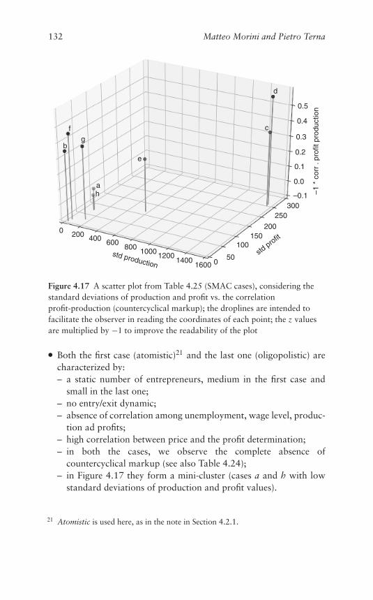
132 Matteo Morini and Pietro Terna
0.4
0.3
0.2
0.1
0.0
0.5
–0.1
250
200150
100
50
300
0
b
fg
ah
std production
std profit
–1 *
cor
r . p
rofit
pro
duct
ion
c
e
d
140012001000
800600400200
1600
0
Figure 4.17 A scatter plot from Table 4.25 (SMAC cases), considering thestandard deviations of production and profit vs. the correlationprofit-production (countercyclical markup); the droplines are intended tofacilitate the observer in reading the coordinates of each point; the z valuesare multiplied by −1 to improve the readability of the plot
● Both the first case (atomistic)21 and the last one (oligopolistic) arecharacterized by:– a static number of entrepreneurs, medium in the first case and
small in the last one;– no entry/exit dynamic;– absence of correlation among unemployment, wage level, produc-
tion ad profits;– high correlation between price and the profit determination;– in both the cases, we observe the complete absence of
countercyclical markup (see also Table 4.24);– in Figure 4.17 they form a mini-cluster (cases a and h with low
standard deviations of production and profit values).
21 Atomistic is used here, as in the note in Section 4.2.1.
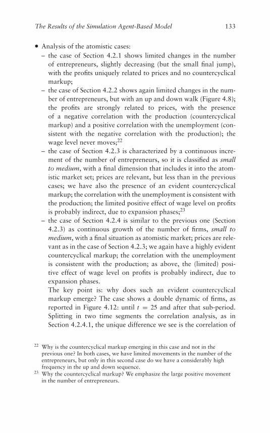
The Results of the Simulation Agent-Based Model 133
● Analysis of the atomistic cases:– the case of Section 4.2.1 shows limited changes in the number
of entrepreneurs, slightly decreasing (but the small final jump),with the profits uniquely related to prices and no countercyclicalmarkup;
– the case of Section 4.2.2 shows again limited changes in the num-ber of entrepreneurs, but with an up and down walk (Figure 4.8);the profits are strongly related to prices, with the presenceof a negative correlation with the production (countercyclicalmarkup) and a positive correlation with the unemployment (con-sistent with the negative correlation with the production); thewage level never moves;22
– the case of Section 4.2.3 is characterized by a continuous incre-ment of the number of entrepreneurs, so it is classified as smallto medium, with a final dimension that includes it into the atom-istic market set; prices are relevant, but less than in the previouscases; we have also the presence of an evident countercyclicalmarkup; the correlation with the unemployment is consistent withthe production; the limited positive effect of wage level on profitsis probably indirect, due to expansion phases;23
– the case of Section 4.2.4 is similar to the previous one (Section4.2.3) as continuous growth of the number of firms, small tomedium, with a final situation as atomistic market; prices are rele-vant as in the case of Section 4.2.3; we again have a highly evidentcountercyclical markup; the correlation with the unemploymentis consistent with the production; as above, the (limited) posi-tive effect of wage level on profits is probably indirect, due toexpansion phases.The key point is: why does such an evident countercyclicalmarkup emerge? The case shows a double dynamic of firms, asreported in Figure 4.12: until t = 25 and after that sub-period.Splitting in two time segments the correlation analysis, as inSection 4.2.4.1, the unique difference we see is the correlation of
22 Why is the countercyclical markup emerging in this case and not in theprevious one? In both cases, we have limited movements in the number of theentrepreneurs, but only in this second case do we have a considerably highfrequency in the up and down sequence.
23 Why the countercyclical markup? We emphasize the large positive movementin the number of entrepreneurs.
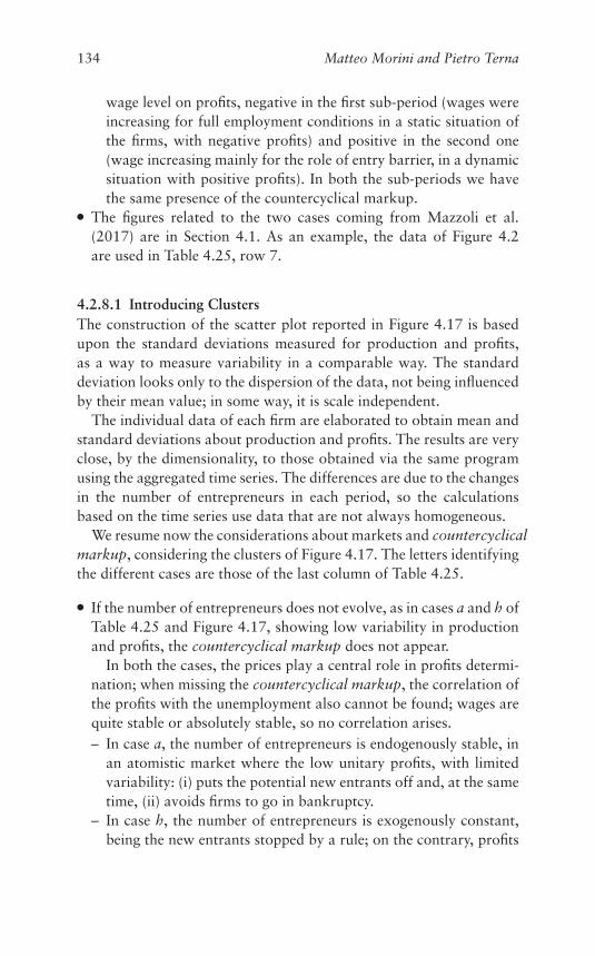
134 Matteo Morini and Pietro Terna
wage level on profits, negative in the first sub-period (wages wereincreasing for full employment conditions in a static situation ofthe firms, with negative profits) and positive in the second one(wage increasing mainly for the role of entry barrier, in a dynamicsituation with positive profits). In both the sub-periods we havethe same presence of the countercyclical markup.
● The figures related to the two cases coming from Mazzoli et al.(2017) are in Section 4.1. As an example, the data of Figure 4.2are used in Table 4.25, row 7.
4.2.8.1 Introducing ClustersThe construction of the scatter plot reported in Figure 4.17 is basedupon the standard deviations measured for production and profits,as a way to measure variability in a comparable way. The standarddeviation looks only to the dispersion of the data, not being influencedby their mean value; in some way, it is scale independent.
The individual data of each firm are elaborated to obtain mean andstandard deviations about production and profits. The results are veryclose, by the dimensionality, to those obtained via the same programusing the aggregated time series. The differences are due to the changesin the number of entrepreneurs in each period, so the calculationsbased on the time series use data that are not always homogeneous.
We resume now the considerations about markets and countercyclicalmarkup, considering the clusters of Figure 4.17. The letters identifyingthe different cases are those of the last column of Table 4.25.
● If the number of entrepreneurs does not evolve, as in cases a and h ofTable 4.25 and Figure 4.17, showing low variability in productionand profits, the countercyclical markup does not appear.
In both the cases, the prices play a central role in profits determi-nation; when missing the countercyclical markup, the correlation ofthe profits with the unemployment also cannot be found; wages arequite stable or absolutely stable, so no correlation arises.– In case a, the number of entrepreneurs is endogenously stable, in
an atomistic market where the low unitary profits, with limitedvariability: (i) puts the potential new entrants off and, at the sametime, (ii) avoids firms to go in bankruptcy.
– In case h, the number of entrepreneurs is exogenously constant,being the new entrants stopped by a rule; on the contrary, profits
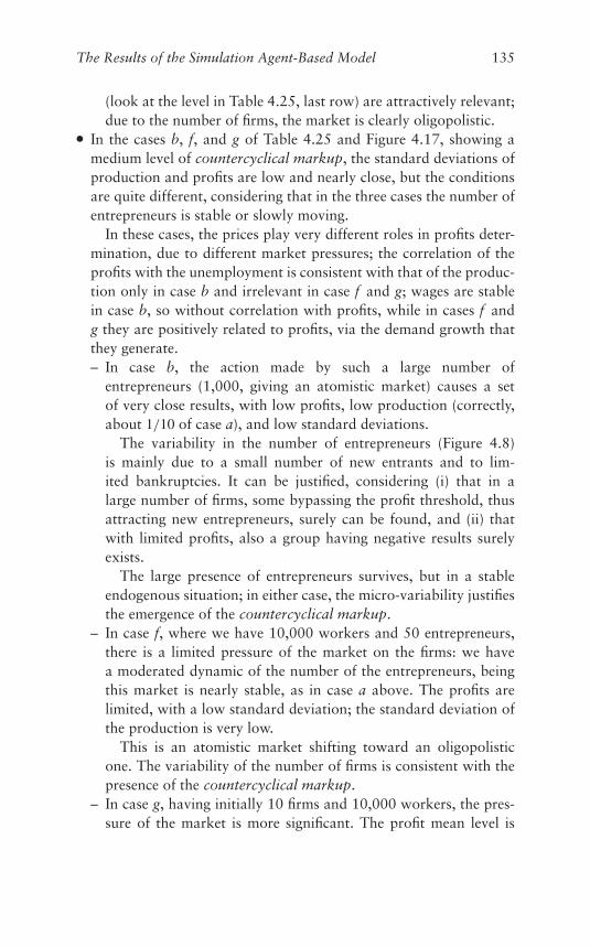
The Results of the Simulation Agent-Based Model 135
(look at the level in Table 4.25, last row) are attractively relevant;due to the number of firms, the market is clearly oligopolistic.
● In the cases b, f, and g of Table 4.25 and Figure 4.17, showing amedium level of countercyclical markup, the standard deviations ofproduction and profits are low and nearly close, but the conditionsare quite different, considering that in the three cases the number ofentrepreneurs is stable or slowly moving.
In these cases, the prices play very different roles in profits deter-mination, due to different market pressures; the correlation of theprofits with the unemployment is consistent with that of the produc-tion only in case b and irrelevant in case f and g; wages are stablein case b, so without correlation with profits, while in cases f andg they are positively related to profits, via the demand growth thatthey generate.– In case b, the action made by such a large number of
entrepreneurs (1,000, giving an atomistic market) causes a setof very close results, with low profits, low production (correctly,about 1/10 of case a), and low standard deviations.
The variability in the number of entrepreneurs (Figure 4.8)is mainly due to a small number of new entrants and to lim-ited bankruptcies. It can be justified, considering (i) that in alarge number of firms, some bypassing the profit threshold, thusattracting new entrepreneurs, surely can be found, and (ii) thatwith limited profits, also a group having negative results surelyexists.
The large presence of entrepreneurs survives, but in a stableendogenous situation; in either case, the micro-variability justifiesthe emergence of the countercyclical markup.
– In case f, where we have 10,000 workers and 50 entrepreneurs,there is a limited pressure of the market on the firms: we havea moderated dynamic of the number of the entrepreneurs, beingthis market is nearly stable, as in case a above. The profits arelimited, with a low standard deviation; the standard deviation ofthe production is very low.
This is an atomistic market shifting toward an oligopolisticone. The variability of the number of firms is consistent with thepresence of the countercyclical markup.
– In case g, having initially 10 firms and 10,000 workers, the pres-sure of the market is more significant. The profit mean level is
136 Matteo Morini and Pietro Terna
negative (losses), but the production shows a greater variability ifcompared with the previous case; the relevance of prices is alsogreater than in case f. We have the presence of the countercyclicalmarkup in an oligopoly.
● In cases c and d of Table 4.25 and Figure 4.17, the number ofthe entrepreneurs is increasing, due to the high pressure of themarket; in both cases, the countercyclical markup is evident. Thestandard deviations of production and profits are relevant, and thischaracteristic is certainly related to the dynamic of the supply side.
In these cases, the prices play an important role in profits deter-mination, due to the market pressure; the correlation of the profitswith unemployment is always consistent with that of production.Wages are positively related to profits, via the demand growth thatthey generate.– In case c, having initially only 10 entrepreneurs and 100,000
workers, the pressure of the market is quite high; wages movefrequently, as they are used as an entry barrier.
– In case d, the initial number of entrepreneurs is 20, but the pres-sure of the market is anyway high, with a lot of new entries(Figure 4.12) and a highly significant countercyclical markup.
● Case e, starting with 50 entrepreneurs and increasing until a level of200, is quite atypical, with a light countercyclical markup and highvariance of profits and production, mainly a high effect of prices.We underline the difference with case b, looking at the standarddeviations.
4.3 A Qualitative Analysis of ASHAM Experiments
In this part of the chapter we explore the complicated, but more real-istic, world of the ASHAM construction. SMAC and ASHAM modesare technically introduced in Section 3.1.2. The ASHAM case usesAppendix A as a source of ideas. We repeat here the same warningprovided in Section 3.1.2: in Appendix A and in Chapter 3 (Figures3.2, 3.3, 3.4, and 3.5), seemingly we have offer curves. Actually, theyare more complicated objects, as on the x-axis we do not have quan-tities, but agents: at the price reported in the y-axis, the agent cansell all the quantity she owns (a unitary quantity, in the simple exam-ples reported in Appendix A and in the quoted figures; any quantity,in the ASHAM case). Specifically, in ASHAM each seller has a true

The Results of the Simulation Agent-Based Model 137
horizontal offer curve: at a given price, she sells any quantity. We donot call it “supply curve” on purpose. The prices reported in the fig-ures are reservation prices for the buyers, while for the sellers theyare close to fixed sell prices like those exposed in a mall. Correct anddescriptive names for both the curves of these figures are buyers’ pricecurve and sellers’ price curve.
We do not reproduce the same synoptic analysis that we built forSMAC, where the market structures and the countercyclical markupphenomenon have been emerging. We now follow a fine grained-qualitative search for realistic way of behaving in price formation,keeping in mind the strong hypothesis in Chapter 2 about priceheterogeneity among firms.
Doing that with the ASHAM scheme, we are outside the too mech-anistic perspective of the SMAC construction, built on a too simpleand abstract process of price formation.
We have four different implementations of the ASHAM world:
● in Section 4.4, the full ASHAM, introduced in Section 3.1.2, as aparadigm with continuous price adaptation, on both the side ofthe sellers (firms-entrepreneurs) and of the buyers (workers andentrepreneurs, as consumers); the price adaptation is related to pricechanges, if any, in each sub-step of each cycle, or time step, asexplained in Section 3.7; within this paradigm, we have also theoption of random corrections pushing up the prices (as actions ofthe sellers, related to information shocks);
● in Section 4.5, the quasi ASHAM with the unsold option; the quasispecification is introduced in Section 3.1.2, as a paradigm with theseller prices adapting only at the beginning of each period (cycle ofthe simulation); the unsold option is introduced in Section 3.10.2 asa behavior of the entrepreneurs modifying their prices at the end ofa period for the next one, if they have unsold production;
● in Section 4.6, the quasi ASHAM, with the randomUp option; asabove, the quasi specification is introduced in Section 3.1.2, as aparadigm with the seller prices adapting only at the beginning ofeach period (cycle of the simulation); the random up option is intro-duced in Section 3.10.2 as a behavior of the entrepreneurs increasingtheir prices at the end of a period for the next one, in a seem-ingly random way, that we can imagine to be related to informationshocks, as indicated previously;
138 Matteo Morini and Pietro Terna
● in Section 4.7, the quasi ASHAM, with the profit option; as above,the quasi specification is introduced in Section 3.1.2, as a paradigmwith the seller prices adapting only at the beginning of each period(cycle of the simulation); the profit option is introduced in Section3.10.2 as a behavior of the entrepreneurs increasing or decreas-ing their prices at the end of a period for the next one, tryingto recover a falling profit. To summarize the actual difficulty ofknowing the demand elasticity, the actual choice between raisingor lowering the price is a random one, with 60% of probabil-ity to the first choice (“raise”) and 40% to the other one, ifpriceSwitchIfProfitFalls is set to “raise” and vice versa ifit set to “lower.”
4.4 Full ASHAM
4.4.1 Case 7: 10 Entrepreneurs and 10,000 Workers, in aStable Economy, with an Increasing Number of Firms
We start the exploration of our peculiar ASHAM economics with asimple case on the edge of stability, with micro-movements within thedata series. The sets of the parameters of the experiment are reportedin Tables B.3 and B.4 of Appendix B. Table B.2 reports all the defini-tions and the links to the sections where the variables are introducedand explained, in Chapter 3. Each case requires the input of a fewparameters in an interactive way: we report them in Table C.1 ofAppendix C.
● The case starts with:– 10 entrepreneurs and 10,000 workers;– an initial distribution of the prices of the agents based on a
choice of the parameters of Section 3.6 (related to the Item 6of the model outline of Figure 3.1, and specifically to the func-tion setInitialPricesHM), with the purpose of generating aninitial situation like that of Figure 3.3, with two not overlappingdistributions of the reservation prices.24
We specify such kind of situation with the parameter initShiftset to −0.15 and the parameter initShock set to 0.10.
24 The max price a buyer could pay and the min one a seller could accept. Forsellers, these prices are close to sell prices like those exposed in a mall.
The Results of the Simulation Agent-Based Model 139
● The second relevant choice is that of having the parameterrunningShockB, for the buyers, set to 0.2 and runningShockS,for the sellers, to 0.05. In this way, both the buyers and the sellersquickly adapt their prices to make deals.
Following Section A.4.1.3 of Appendix A, the winners are thesellers, acting with a slow pace of price correction, as they wouldcherry-pick the best buyers (those with the higher reservation price).In this way, they avoid contributing to the fall of the prices. Thisbehavior is consistent with the usual description of the sell prices assticky, where sticky is a general economics term that, when appliedto the sell prices, means that the firms are reluctant to change theirprices also in the presence of modifications in input cost or demandquantities.25
The cherry-picking process is not related always to the same buy-ers, because with the sequence of sub-steps within each time step, asexplained in Section 3.7, we are adopting the solution of the SectionA.5.2 of Appendix A: due to the continuous price corrections, thebuy action are quite uncertain and in the about 50% of the cases theagents fail to buy, but as we repeat the buy-sell session several timesin each cycle or time step, the failing agents are never the same. Ineach sub-step, (i) the buyers meet different sellers, generating theprice information diffusion process via successful deals, and (ii) theagents actually buying change continuously.
● Considering the Q parameter of Section 3.2.2, the entrepreneurs, toplan their productions, weight 50% the consumption sat time t − 1and 50% those at time t − 2, introducing some delays in productionadaptation.
Given the initial construction of the prices, we have the expec-tation of (i) a moderate positive level of the profits with (ii) thepossibility of a lack of consumption (high prices) and (iii) of arising unemployment (low production, as a consequence of theconsumption level): a recessive perspective, in short. We can con-trol it via the level of welfare compensations (with the parametersocialWelfareCompensation set to 0.7, in the presence of a wage
25 The whole set of the parameters of the experiment is reported in Tables B.3and B.4 of Appendix B. Each case requires the input of a few parameters in aninteractive way. We report them in Table C.1 of Appendix C.
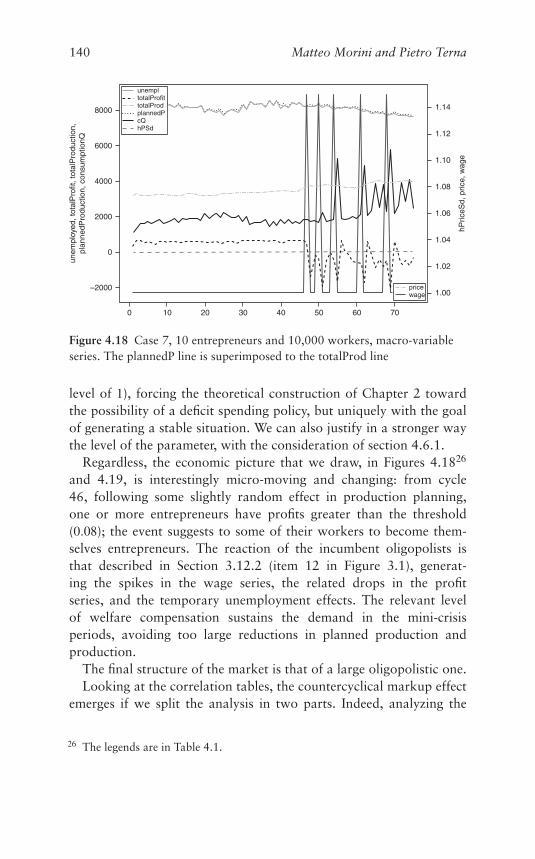
140 Matteo Morini and Pietro Terna
unempltotalProfittotalProdplannedPcQ
wageprice
1.00
0
2000
0
4000
6000
8000
unem
ploy
ed, t
otal
Pro
fit, t
otal
Pro
duct
ion,
plan
nedP
rodu
ctio
n, c
onsu
mpt
ionQ
hPric
eSd,
pric
e, w
age
–2000
10 20 30 40 50 60 70
1.02
1.04
1.06
1.08
1.10
1.12
1.14
hPSd
Figure 4.18 Case 7, 10 entrepreneurs and 10,000 workers, macro-variableseries. The plannedP line is superimposed to the totalProd line
level of 1), forcing the theoretical construction of Chapter 2 towardthe possibility of a deficit spending policy, but uniquely with the goalof generating a stable situation. We can also justify in a stronger waythe level of the parameter, with the consideration of section 4.6.1.
Regardless, the economic picture that we draw, in Figures 4.1826
and 4.19, is interestingly micro-moving and changing: from cycle46, following some slightly random effect in production planning,one or more entrepreneurs have profits greater than the threshold(0.08); the event suggests to some of their workers to become them-selves entrepreneurs. The reaction of the incumbent oligopolists isthat described in Section 3.12.2 (item 12 in Figure 3.1), generat-ing the spikes in the wage series, the related drops in the profitseries, and the temporary unemployment effects. The relevant levelof welfare compensation sustains the demand in the mini-crisisperiods, avoiding too large reductions in planned production andproduction.
The final structure of the market is that of a large oligopolistic one.Looking at the correlation tables, the countercyclical markup effect
emerges if we split the analysis in two parts. Indeed, analyzing the
26 The legends are in Table 4.1.
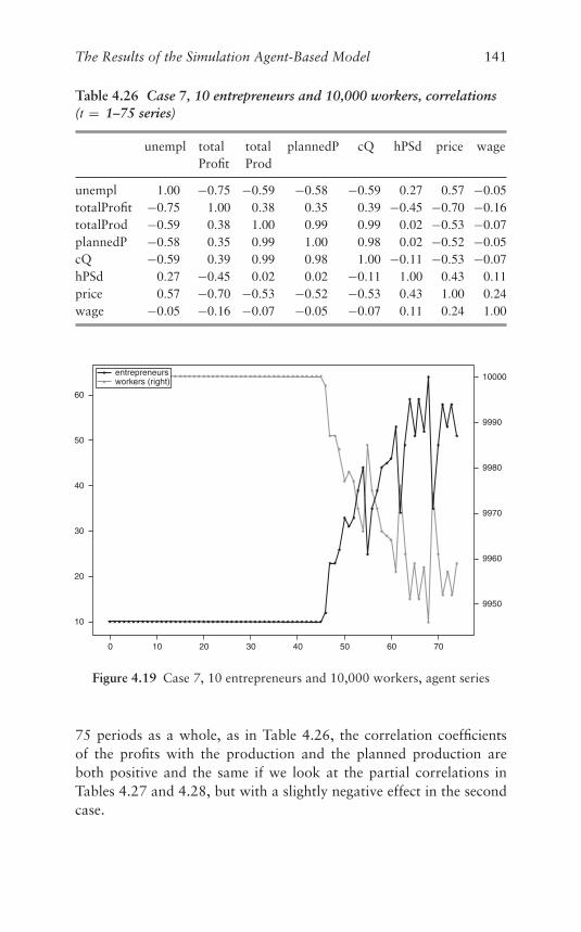
The Results of the Simulation Agent-Based Model 141
Table 4.26 Case 7, 10 entrepreneurs and 10,000 workers, correlations(t = 1–75 series)
unempl totalProfit
totalProd
plannedP cQ hPSd price wage
unempl 1.00 −0.75 −0.59 −0.58 −0.59 0.27 0.57 −0.05totalProfit −0.75 1.00 0.38 0.35 0.39 −0.45 −0.70 −0.16totalProd −0.59 0.38 1.00 0.99 0.99 0.02 −0.53 −0.07plannedP −0.58 0.35 0.99 1.00 0.98 0.02 −0.52 −0.05cQ −0.59 0.39 0.99 0.98 1.00 −0.11 −0.53 −0.07hPSd 0.27 −0.45 0.02 0.02 −0.11 1.00 0.43 0.11price 0.57 −0.70 −0.53 −0.52 −0.53 0.43 1.00 0.24wage −0.05 −0.16 −0.07 −0.05 −0.07 0.11 0.24 1.00
10000
9990
9980
9970
9960
9950
706050403020100
10
20
30
40
50
60
entrepreneursworkers (right)
Figure 4.19 Case 7, 10 entrepreneurs and 10,000 workers, agent series
75 periods as a whole, as in Table 4.26, the correlation coefficientsof the profits with the production and the planned production areboth positive and the same if we look at the partial correlations inTables 4.27 and 4.28, but with a slightly negative effect in the secondcase.
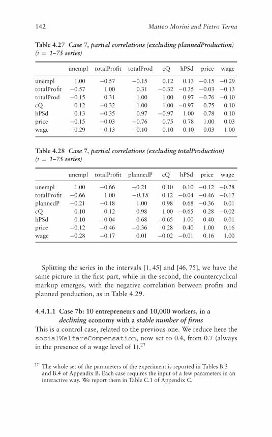
142 Matteo Morini and Pietro Terna
Table 4.27 Case 7, partial correlations (excluding plannedProduction)(t = 1–75 series)
unempl totalProfit totalProd cQ hPSd price wage
unempl 1.00 −0.57 −0.15 0.12 0.13 −0.15 −0.29totalProfit −0.57 1.00 0.31 −0.32 −0.35 −0.03 −0.13totalProd −0.15 0.31 1.00 1.00 0.97 −0.76 −0.10cQ 0.12 −0.32 1.00 1.00 −0.97 0.75 0.10hPSd 0.13 −0.35 0.97 −0.97 1.00 0.78 0.10price −0.15 −0.03 −0.76 0.75 0.78 1.00 0.03wage −0.29 −0.13 −0.10 0.10 0.10 0.03 1.00
Table 4.28 Case 7, partial correlations (excluding totalProduction)(t = 1–75 series)
unempl totalProfit plannedP cQ hPSd price wage
unempl 1.00 −0.66 −0.21 0.10 0.10 −0.12 −0.28totalProfit −0.66 1.00 −0.18 0.12 −0.04 −0.46 −0.17plannedP −0.21 −0.18 1.00 0.98 0.68 −0.36 0.01cQ 0.10 0.12 0.98 1.00 −0.65 0.28 −0.02hPSd 0.10 −0.04 0.68 −0.65 1.00 0.40 −0.01price −0.12 −0.46 −0.36 0.28 0.40 1.00 0.16wage −0.28 −0.17 0.01 −0.02 −0.01 0.16 1.00
Splitting the series in the intervals [1, 45] and [46, 75], we have thesame picture in the first part, while in the second, the countercyclicalmarkup emerges, with the negative correlation between profits andplanned production, as in Table 4.29.
4.4.1.1 Case 7b: 10 entrepreneurs and 10,000 workers, in adeclining economy with a stable number of firms
This is a control case, related to the previous one. We reduce here thesocialWelfareCompensation, now set to 0.4, from 0.7 (alwaysin the presence of a wage level of 1).27
27 The whole set of the parameters of the experiment is reported in Tables B.3and B.4 of Appendix B. Each case requires the input of a few parameters in aninteractive way. We report them in Table C.1 of Appendix C.
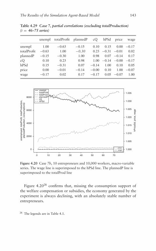
The Results of the Simulation Agent-Based Model 143
Table 4.29 Case 7, partial correlations (excluding totalProduction)(t = 46–75 series)
unempl totalProfit plannedP cQ hPSd price wage
unempl 1.00 −0.63 −0.15 0.10 0.15 0.00 −0.17totalProfit −0.63 1.00 −0.30 0.23 −0.31 −0.01 0.02plannedP −0.15 −0.30 1.00 0.98 0.07 −0.14 0.17cQ 0.10 0.23 0.98 1.00 −0.14 −0.00 −0.17hPSd 0.15 −0.31 0.07 −0.14 1.00 0.10 0.05price 0.00 −0.01 −0.14 −0.00 0.10 1.00 −0.07wage −0.17 0.02 0.17 −0.17 0.05 −0.07 1.00
unempltotalProfittotalProdplannedPcQhPSd
unem
ploy
ed, t
otal
Pro
fit, t
otal
Pro
duct
ion,
plan
nedP
rodu
ctio
n, c
onsu
mpt
ionQ
hPric
eSd,
pric
e, w
age
2000
0
4000
6000
8000
0 10 20 30 40 50 60 70
1.000pricewage
1.005
1.010
1.015
1.020
1.025
1.030
1.035
Figure 4.20 Case 7b, 10 entrepreneurs and 10,000 workers, macro-variableseries. The wage line is superimposed to the hPSd line. The plannedP line issuperimposed to the totalProd line
Figure 4.2028 confirms that, missing the consumption support ofthe welfare compensation or subsidies, the economy generated by theexperiment is always declining, with an absolutely stable number ofentrepreneurs.
28 The legends are in Table 4.1.
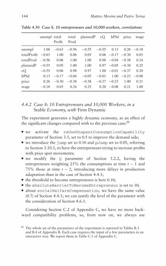
144 Matteo Morini and Pietro Terna
Table 4.30 Case 8, 10 entrepreneurs and 10,000 workers, correlations
unempl totalProfit
totalProd
plannedP cQ hPSd price wage
unempl 1.00 −0.63 −0.56 −0.55 −0.55 0.13 0.26 −0.18
totalProfit −0.63 1.00 0.06 0.05 0.06 −0.17 −0.30 0.03
totalProd −0.56 0.06 1.00 1.00 0.98 −0.04 −0.38 0.24
plannedP −0.55 0.05 1.00 1.00 0.97 −0.05 −0.38 0.25
cQ −0.55 0.06 0.98 0.97 1.00 −0.01 −0.37 0.20
hPSd 0.13 −0.17 −0.04 −0.05 −0.01 1.00 −0.23 −0.08
price 0.26 −0.30 −0.38 −0.38 −0.37 −0.23 1.00 0.21
wage −0.18 0.03 0.24 0.25 0.20 −0.08 0.21 1.00
4.4.2 Case 8: 10 Entrepreneurs and 10,000 Workers, in aStable Economy, with Firm Dynamic
The experiment generates a highly dynamic economy, as an effect ofthe significant changes compared with to the previous case:29
● we activate the reUseUnspentConsumptionCapabilityparameter of Section 3.5, set to 0.5 to improve the demand side;
● we introduce the jump set to 0.10 and pJump set to 0.05, referringto Section 3.10.1, to have the entrepreneurs trying to increase profitswith price spot movements;
● we modify the Q parameter of Section 3.2.2, having theentrepreneurs weighting 25% the consumptions at time t − 1 and75% those at time t − 2, introducing more delays in productionadaptation than in the case of Section 4.4.1;
● the threshold to become entrepreneurs is here 0.10;● the absoluteBarrierToBecomeEntrepreneur is set to 10;● about socialWelfareCompensation, we have the same value
(0.7) of Section 4.4.1; we can justify the level of the parameter withthe consideration of Section 4.6.1.
Considering Section C.2 of Appendix C, we have no more back-ward compatibility problems, so, from now on, we always use
29 The whole set of the parameters of the experiment is reported in Tables B.3and B.4 of Appendix B. Each case requires the input of a few parameters in aninteractive way. We report them in Table C.1 of Appendix C.
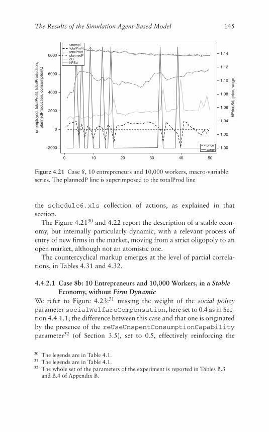
The Results of the Simulation Agent-Based Model 145
unempltotalProfittotalProdplannedPcQ
wageprice
hPSd
8000
6000
4000
2000
0
–2000
0 10 20 30 40 50
1.00
1.02
1.04
1.06
1.08
1.10
1.12
1.14
unem
ploy
ed, t
otal
Pro
fit, t
otal
Pro
duct
ion,
plan
nedP
rodu
ctio
n, c
onsu
mpt
ionQ
hPric
eSd,
pric
e, w
age
Figure 4.21 Case 8, 10 entrepreneurs and 10,000 workers, macro-variableseries. The plannedP line is superimposed to the totalProd line
the schedule6.xls collection of actions, as explained in thatsection.
The Figure 4.2130 and 4.22 report the description of a stable econ-omy, but internally particularly dynamic, with a relevant process ofentry of new firms in the market, moving from a strict oligopoly to anopen market, although not an atomistic one.
The countercyclical markup emerges at the level of partial correla-tions, in Tables 4.31 and 4.32.
4.4.2.1 Case 8b: 10 Entrepreneurs and 10,000 Workers, in a StableEconomy, without Firm Dynamic
We refer to Figure 4.23:31 missing the weight of the social policyparameter socialWelfareCompensation, here set to 0.4 as in Sec-tion 4.4.1.1; the difference between this case and that one is originatedby the presence of the reUseUnspentConsumptionCapabilityparameter32 (of Section 3.5), set to 0.5, effectively reinforcing the
30 The legends are in Table 4.1.31 The legends are in Table 4.1.32 The whole set of the parameters of the experiment is reported in Tables B.3
and B.4 of Appendix B.
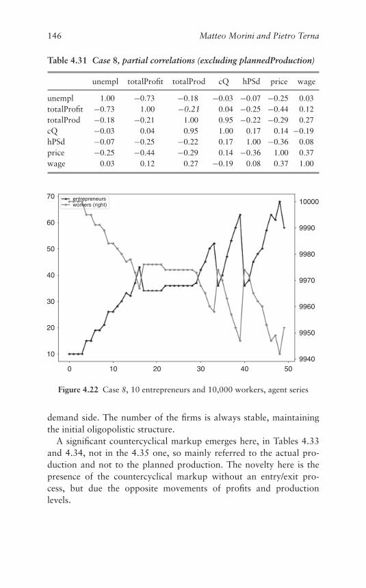
146 Matteo Morini and Pietro Terna
Table 4.31 Case 8, partial correlations (excluding plannedProduction)
unempl totalProfit totalProd cQ hPSd price wage
unempl 1.00 −0.73 −0.18 −0.03 −0.07 −0.25 0.03totalProfit −0.73 1.00 −0.21 0.04 −0.25 −0.44 0.12totalProd −0.18 −0.21 1.00 0.95 −0.22 −0.29 0.27cQ −0.03 0.04 0.95 1.00 0.17 0.14 −0.19hPSd −0.07 −0.25 −0.22 0.17 1.00 −0.36 0.08price −0.25 −0.44 −0.29 0.14 −0.36 1.00 0.37wage 0.03 0.12 0.27 −0.19 0.08 0.37 1.00
entrepreneursworkers (right)
70
60
50
40
30
0 10 20 30 40 509940
9950
9960
10000
9990
9980
9970
20
10
Figure 4.22 Case 8, 10 entrepreneurs and 10,000 workers, agent series
demand side. The number of the firms is always stable, maintainingthe initial oligopolistic structure.
A significant countercyclical markup emerges here, in Tables 4.33and 4.34, not in the 4.35 one, so mainly referred to the actual pro-duction and not to the planned production. The novelty here is thepresence of the countercyclical markup without an entry/exit pro-cess, but due the opposite movements of profits and productionlevels.
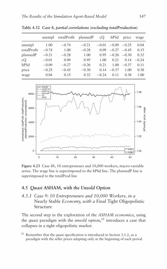
The Results of the Simulation Agent-Based Model 147
Table 4.32 Case 8, partial correlations (excluding totalProduction)
unempl totalProfit plannedP cQ hPSd price wage
unempl 1.00 −0.74 −0.21 −0.01 −0.09 −0.25 0.04totalProfit −0.74 1.00 −0.28 0.09 −0.27 −0.45 0.15plannedP −0.21 −0.28 1.00 0.95 −0.26 −0.30 0.32cQ −0.01 0.09 0.95 1.00 0.21 0.14 −0.24hPSd −0.09 −0.27 −0.26 0.21 1.00 −0.37 0.11price −0.25 −0.45 −0.30 0.14 −0.37 1.00 0.38wage 0.04 0.15 0.32 −0.24 0.11 0.38 1.00
8000
6000
4000
2000
0
0 10 20 30 40 50
1.00
1.02
1.04
1.06
1.08
unem
ploy
ed, t
otal
Pro
fit, t
otal
Pro
duct
ion,
plan
nedP
rodu
ctio
n, c
onsu
mpt
ionQ
hPric
eSd,
pric
e, w
age
unempltotalProfittotalProdplannedPcQ
wageprice
hPSd
Figure 4.23 Case 8b, 10 entrepreneurs and 10,000 workers, macro-variableseries. The wage line is superimposed to the hPSd line. The plannedP line issuperimposed to the totalProd line
4.5 Quasi ASHAM, with the Unsold Option
4.5.1 Case 9: 10 Entrepreneurs and 10,000 Workers, in aNearly Stable Economy, with a Final Tight OligopolisticStructure
The second step in the exploration of the ASHAM economics, usingthe quasi paradigm with the unsold option,33 introduces a case thatcollapses in a tight oligopolistic market.
33 Remember that the quasi specification is introduced in Section 3.1.2, as aparadigm with the seller prices adapting only at the beginning of each period
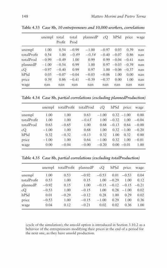
148 Matteo Morini and Pietro Terna
Table 4.33 Case 8b, 10 entrepreneurs and 10,000 workers, correlations
unempl totalProfit
totalProd
plannedP cQ hPSd price wage
unempl 1.00 0.54 −0.99 −1.00 −0.97 0.03 0.39 nantotalProfit 0.54 1.00 −0.49 −0.54 −0.40 −0.07 0.86 nantotalProd −0.99 −0.49 1.00 0.99 0.99 −0.04 −0.41 nanplannedP −1.00 −0.54 0.99 1.00 0.97 −0.03 −0.39 nancQ −0.97 −0.40 0.99 0.97 1.00 −0.06 −0.37 nanhPSd 0.03 −0.07 −0.04 −0.03 −0.06 1.00 0.00 nanprice 0.39 0.86 −0.41 −0.39 −0.37 0.00 1.00 nanwage nan nan nan nan nan nan nan nan
Table 4.34 Case 8b, partial correlations (excluding plannedProduction)
unempl totalProfit totalProd cQ hPSd price wage
unempl 1.00 1.00 0.63 −1.00 0.32 −1.00 0.00totalProfit 1.00 1.00 −0.65 1.00 −0.32 1.00 −0.04totalProd 0.63 −0.65 1.00 0.68 −0.13 0.64 −0.00cQ −1.00 1.00 0.68 1.00 0.32 −1.00 −0.20hPSd 0.32 −0.32 −0.13 0.32 1.00 0.32 0.00price −1.00 1.00 0.64 −1.00 0.32 1.00 −0.01wage 0.00 −0.04 −0.00 −0.20 0.00 −0.01 1.00
Table 4.35 Case 8b, partial correlations (excluding totalProduction)
unempl totalProfit plannedP cQ hPSd price wage
unempl 1.00 0.53 −0.92 −0.53 0.01 −0.53 0.04totalProfit 0.53 1.00 0.15 1.00 −0.29 1.00 0.12plannedP −0.92 0.15 1.00 −0.15 −0.12 −0.15 −0.21cQ −0.53 1.00 −0.15 1.00 0.28 −1.00 0.02hPSd 0.01 −0.29 −0.12 0.28 1.00 0.29 0.02price −0.53 1.00 −0.15 −1.00 0.29 1.00 0.36wage 0.04 0.12 −0.21 0.02 0.02 0.36 1.00
(cycle of the simulation); the unsold option is introduced in Section 3.10.2 as abehavior of the entrepreneurs modifying their prices at the end of a period forthe next one, as they have unsold production.
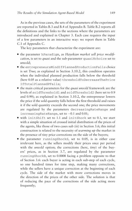
The Results of the Simulation Agent-Based Model 149
As in the previous cases, the sets of the parameters of the experimentare reported in Tables B.3 and B.4 of Appendix B. Table B.2 reports allthe definitions and the links to the sections where the parameters areintroduced and explained in Chapter 3. Each case requires the inputof a few parameters in an interactive way: we report them in TableC.1 of Appendix C.
The key parameters that characterize the experiment are:
● the parameter hParadigm, as Hayekian market sell price modifi-cation, is set to quasi and the sub-parameter quasiHchoice set tounsold;
● the entrepreneursMindIfPlannedProductionFalls choiceis set True; as explained in Section 3.10.2, this condition operateswhen the individual planned production falls below the threshold(here 0.05 as a relative value) thresholdToDecreaseThePriceIfTotalPlannedPFalls;
● the main critical parameters for the quasi unsold framework are thelevels of soldThreshold1 and soldThreshold2 (here set to 0.9and 0.99); as explained in Section 3.10.2, the entrepreneur lowersthe price if the sold quantity falls below the first threshold and raisesit if the sold quantity exceeds the second one; the price movementsare regulated by the parameters decreasingRateRange andincreasingRateRange, set to −0.1 and 0.01;
● with initShift set to 1.1 and initShock set to 0.1, we startwith a simple situation of crossed initial distribution of the prices ofthe agents, like those of two cases sub (iii) in Section 3.6; this initialconstruction is related to the necessity of warming up the market inthe presence of tiny price corrections on the side of the buyers;
● the parameter runningShockS, set to 0.05, is in either caseirrelevant here, as the sellers modify their prices once per periodwith the unsold option; the corrections (here, tiny) of the buy-ers’ prices, as in Section 3.7, are regulated by the parameterrunningShockB, set to 0.0008 facing a problem opposite to thatof Section 3.6: each buyer is acting in each sub-step of each cycle,so one hundred times for time step, making many corrections,while the sellers have a unique correction at the beginning of eachcycle. The side of the market with more corrections moves inthe direction of the prices of the other side. The solution is thatof reducing the pace of the corrections of the side acting morefrequently;
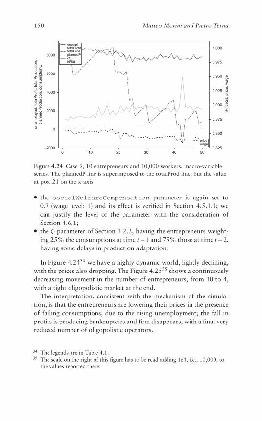
150 Matteo Morini and Pietro Terna
8000
6000
4000
2000
0
–200010 40 5030200
0.900
hPric
eSd,
pric
e, w
age
1.000
0.975
0.950
0.925
0.875
0.850
0.825
unem
ploy
ed, t
otal
Pro
fit, t
otal
Pro
duct
ion,
plan
nedP
rodu
ctio
n, c
onsu
mpt
ionQ
unempltotalProfittotalProdplannedPcQ
wageprice
hPSd
Figure 4.24 Case 9, 10 entrepreneurs and 10,000 workers, macro-variableseries. The plannedP line is superimposed to the totalProd line, but the valueat pos. 21 on the x-axis
● the socialWelfareCompensation parameter is again set to0.7 (wage level: 1) and its effect is verified in Section 4.5.1.1; wecan justify the level of the parameter with the consideration ofSection 4.6.1;
● the Q parameter of Section 3.2.2, having the entrepreneurs weight-ing 25% the consumptions at time t −1 and 75% those at time t −2,having some delays in production adaptation.
In Figure 4.2434 we have a highly dynamic world, lightly declining,with the prices also dropping. The Figure 4.2535 shows a continuouslydecreasing movement in the number of entrepreneurs, from 10 to 4,with a tight oligopolistic market at the end.
The interpretation, consistent with the mechanism of the simula-tion, is that the entrepreneurs are lowering their prices in the presenceof falling consumptions, due to the rising unemployment; the fall inprofits is producing bankruptcies and firm disappears, with a final veryreduced number of oligopolistic operators.
34 The legends are in Table 4.1.35 The scale on the right of this figure has to be read adding 1e4, i.e., 10,000, to
the values reported there.
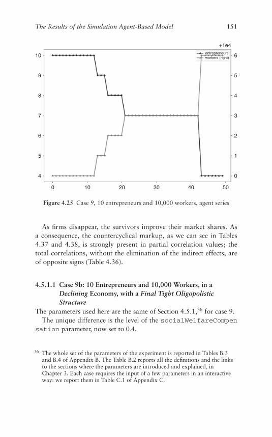
The Results of the Simulation Agent-Based Model 151
entrepreneursworkers (right)
+1e4
6
5
4
3
2
1
0
504030200
5
4
6
7
8
9
10
10
Figure 4.25 Case 9, 10 entrepreneurs and 10,000 workers, agent series
As firms disappear, the survivors improve their market shares. Asa consequence, the countercyclical markup, as we can see in Tables4.37 and 4.38, is strongly present in partial correlation values; thetotal correlations, without the elimination of the indirect effects, areof opposite signs (Table 4.36).
4.5.1.1 Case 9b: 10 Entrepreneurs and 10,000 Workers, in aDeclining Economy, with a Final Tight OligopolisticStructure
The parameters used here are the same of Section 4.5.1,36 for case 9.The unique difference is the level of the socialWelfareCompen
sation parameter, now set to 0.4.
36 The whole set of the parameters of the experiment is reported in Tables B.3and B.4 of Appendix B. The Table B.2 reports all the definitions and the linksto the sections where the parameters are introduced and explained, inChapter 3. Each case requires the input of a few parameters in an interactiveway: we report them in Table C.1 of Appendix C.
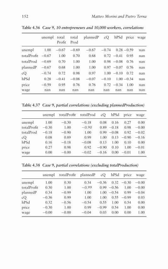
152 Matteo Morini and Pietro Terna
Table 4.36 Case 9, 10 entrepreneurs and 10,000 workers, correlations
unempl totalProfit
totalProd
plannedP cQ hPSd price wage
unempl 1.00 −0.67 −0.69 −0.67 −0.74 0.28 −0.59 nan
totalProfit −0.67 1.00 0.70 0.68 0.72 −0.41 0.95 nan
totalProd −0.69 0.70 1.00 1.00 0.98 −0.08 0.76 nan
plannedP −0.67 0.68 1.00 1.00 0.97 −0.07 0.76 nan
cQ −0.74 0.72 0.98 0.97 1.00 −0.10 0.72 nan
hPSd 0.28 −0.41 −0.08 −0.07 −0.10 1.00 −0.34 nan
price −0.59 0.95 0.76 0.76 0.72 −0.34 1.00 nanwage nan nan nan nan nan nan nan nan
Table 4.37 Case 9, partial correlations (excluding plannedProduction)
unempl totalProfit totalProd cQ hPSd price wage
unempl 1.00 −0.30 −0.18 0.08 0.16 0.27 0.00totalProfit −0.30 1.00 −0.90 0.89 −0.18 0.98 −0.00totalProd −0.18 −0.90 1.00 0.99 −0.08 0.92 −0.02cQ 0.08 0.89 0.99 1.00 0.13 −0.90 −0.16hPSd 0.16 −0.18 −0.08 0.13 1.00 0.10 0.00price 0.27 0.98 0.92 −0.90 0.10 1.00 −0.01wage 0.00 −0.00 −0.02 −0.16 0.00 −0.01 1.00
Table 4.38 Case 9, partial correlations (excluding totalProduction)
unempl totalProfit plannedP cQ hPSd price wage
unempl 1.00 0.30 0.34 −0.36 0.32 −0.30 −0.00totalProfit 0.30 1.00 −0.99 0.99 −0.56 1.00 −0.00plannedP 0.34 −0.99 1.00 1.00 −0.54 0.99 −0.04cQ −0.36 0.99 1.00 1.00 0.55 −0.99 0.03hPSd 0.32 −0.56 −0.54 0.55 1.00 0.54 0.00price −0.30 1.00 0.99 −0.99 0.54 1.00 0.00wage −0.00 −0.00 −0.04 0.03 0.00 0.00 1.00
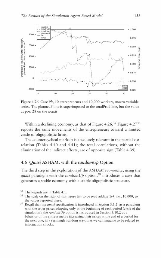
The Results of the Simulation Agent-Based Model 153
8000
6000
4000
2000
–2000
10 40 5030200
0
0.900
hPric
eSd,
pric
e, w
age
1.000
0.975
0.950
0.925
0.875
0.850
0.825
unem
ploy
ed, t
otal
Pro
fit, t
otal
Pro
duct
ion,
plan
nedP
rodu
ctio
n, c
onsu
mpt
ionQ
unempltotalProfittotalProdplannedPcQ
wageprice
hPSd
Figure 4.26 Case 9b, 10 entrepreneurs and 10,000 workers, macro-variableseries. The plannedP line is superimposed to the totalProd line, but the valueat pos. 28 on the x-axis
Within a declining economy, as that of Figure 4.26,37 Figure 4.2738
reports the same movements of the entrepreneurs toward a limitedcircle of oligopolistic firms.
The countercyclical markup is absolutely relevant in the partial cor-relation (Tables 4.40 and 4.41); the total correlations, without theelimination of the indirect effects, are of opposite sign (Table 4.39).
4.6 Quasi ASHAM, with the randomUp Option
The third step in the exploration of the ASHAM economics, using thequasi paradigm with the randomUp option,39 introduces a case thatgenerates a stable economy with a stable oligopolistic structure.
37 The legends are in Table 4.1.38 The scale on the right of this figure has to be read adding 1e4, i.e., 10,000, to
the values reported there.39 Recall that the quasi specification is introduced in Section 3.1.2, as a paradigm
with the seller prices adapting only at the beginning of each period (cycle of thesimulation); the randomUp option is introduced in Section 3.10.2 as abehavior of the entrepreneurs increasing their prices at the end of a period forthe next one, in a seemingly random way, that we can imagine to be related toinformation shocks.
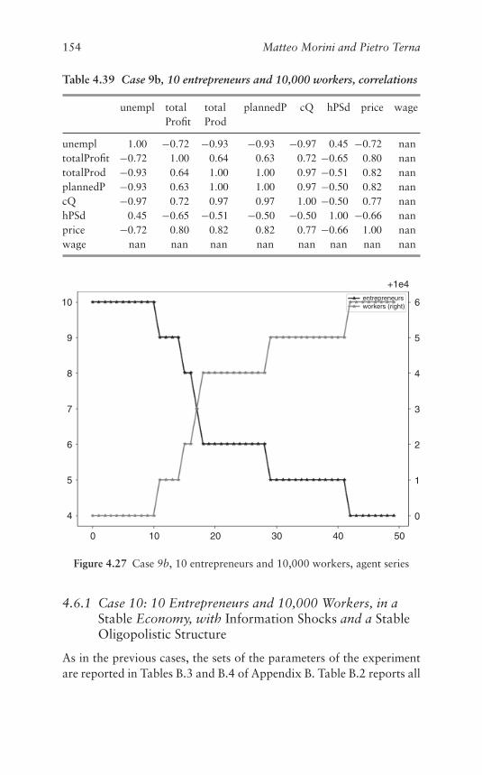
154 Matteo Morini and Pietro Terna
Table 4.39 Case 9b, 10 entrepreneurs and 10,000 workers, correlations
unempl totalProfit
totalProd
plannedP cQ hPSd price wage
unempl 1.00 −0.72 −0.93 −0.93 −0.97 0.45 −0.72 nantotalProfit −0.72 1.00 0.64 0.63 0.72 −0.65 0.80 nantotalProd −0.93 0.64 1.00 1.00 0.97 −0.51 0.82 nanplannedP −0.93 0.63 1.00 1.00 0.97 −0.50 0.82 nancQ −0.97 0.72 0.97 0.97 1.00 −0.50 0.77 nanhPSd 0.45 −0.65 −0.51 −0.50 −0.50 1.00 −0.66 nanprice −0.72 0.80 0.82 0.82 0.77 −0.66 1.00 nanwage nan nan nan nan nan nan nan nan
entrepreneursworkers (right)
+1e4
6
5
4
3
2
1
0
504030200 10
5
4
6
7
8
9
10
Figure 4.27 Case 9b, 10 entrepreneurs and 10,000 workers, agent series
4.6.1 Case 10: 10 Entrepreneurs and 10,000 Workers, in aStable Economy, with Information Shocks and a StableOligopolistic Structure
As in the previous cases, the sets of the parameters of the experimentare reported in Tables B.3 and B.4 of Appendix B. Table B.2 reports all
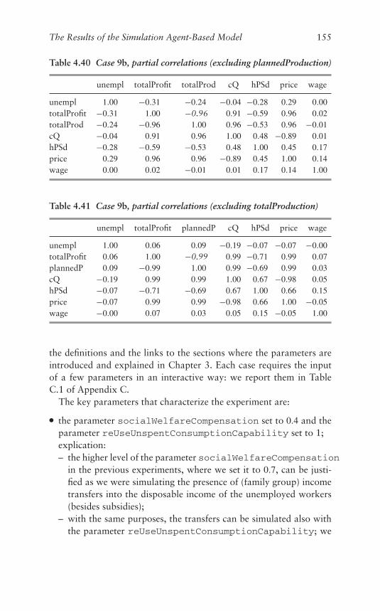
The Results of the Simulation Agent-Based Model 155
Table 4.40 Case 9b, partial correlations (excluding plannedProduction)
unempl totalProfit totalProd cQ hPSd price wage
unempl 1.00 −0.31 −0.24 −0.04 −0.28 0.29 0.00totalProfit −0.31 1.00 −0.96 0.91 −0.59 0.96 0.02totalProd −0.24 −0.96 1.00 0.96 −0.53 0.96 −0.01cQ −0.04 0.91 0.96 1.00 0.48 −0.89 0.01hPSd −0.28 −0.59 −0.53 0.48 1.00 0.45 0.17price 0.29 0.96 0.96 −0.89 0.45 1.00 0.14wage 0.00 0.02 −0.01 0.01 0.17 0.14 1.00
Table 4.41 Case 9b, partial correlations (excluding totalProduction)
unempl totalProfit plannedP cQ hPSd price wage
unempl 1.00 0.06 0.09 −0.19 −0.07 −0.07 −0.00totalProfit 0.06 1.00 −0.99 0.99 −0.71 0.99 0.07plannedP 0.09 −0.99 1.00 0.99 −0.69 0.99 0.03cQ −0.19 0.99 0.99 1.00 0.67 −0.98 0.05hPSd −0.07 −0.71 −0.69 0.67 1.00 0.66 0.15price −0.07 0.99 0.99 −0.98 0.66 1.00 −0.05wage −0.00 0.07 0.03 0.05 0.15 −0.05 1.00
the definitions and the links to the sections where the parameters areintroduced and explained in Chapter 3. Each case requires the inputof a few parameters in an interactive way: we report them in TableC.1 of Appendix C.
The key parameters that characterize the experiment are:
● the parameter socialWelfareCompensation set to 0.4 and theparameter reUseUnspentConsumptionCapability set to 1;explication:– the higher level of the parameter socialWelfareCompensation
in the previous experiments, where we set it to 0.7, can be justi-fied as we were simulating the presence of (family group) incometransfers into the disposable income of the unemployed workers(besides subsidies);
– with the same purposes, the transfers can be simulated also withthe parameter reUseUnspentConsumptionCapability; we

156 Matteo Morini and Pietro Terna
8000
10000
6000
4000
2000
0
10 40 5030200
hPric
eSd,
pric
e, w
age
unem
ploy
ed, t
otal
Pro
fit, t
otal
Pro
duct
ion,
plan
nedP
rodu
ctio
n, c
onsu
mpt
ionQ
0.90
0.95
1.00
1.05
1.10unempltotalProfittotalProdplannedPcQ
wageprice
hPSd
Figure 4.28 Case 10, 10 entrepreneurs and 10,000 workers, macro-variableseries. The plannedP line is superimposed to the totalProd line
9.0
9.2
9.4
9.6
9.8
10.0
504030200 10
1.0
0.8
0.6
0.4
0.2
0.0
entrepreneursworkers (right)
+1e4
Figure 4.29 Case 10, 10 entrepreneurs and 10,000 workers, agent series
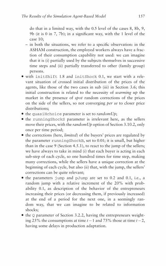
The Results of the Simulation Agent-Based Model 157
do that in a limited way, with the 0.5 level of the cases 8, 8b, 9,9b (it is 0 in 7, 7b); in a significant way, with the 1 level of thecase 10;
– in both the situations, we refer to a specific observation: in theASHAM construction, the employed workers always have a frac-tion of their consumption capability not used: we can imaginethat it is (i) partially used by the subjects themselves in successivetime steps and (ii) partially transferred to other (family group)persons.
● with initShift 1.8 and initShock 0.1, we start with a rele-vant situation of crossed initial distribution of the prices of theagents, like those of the two cases in sub (iii) in Section 3.6; thisinitial construction is related to the necessity of warming up themarket in the presence of spot random corrections of the priceson the side of the sellers, so not converging per se to closer pricedistributions;
● the quasiHchoice parameter is set to randomUp;● the runningShockS parameter is irrelevant here, as the sellers
move their prices, with the randomUp option of Section 3.10.2, onlyonce per time period;
● the corrections (here, limited) of the buyers’ prices are regulated bythe parameter runningShockB, set to 0.01; it is small, but higherthan in the case 9 (Section 4.5.1), to react to the jump of the sellers;we have always to take in mind (i) that each buyer is acting in eachsub-step of each cycle, so one hundred times for time step, makingmany corrections, while the sellers have a unique correction at thebeginning of each cycle, but also (ii) that, with the jump, the sellers’corrections can be quite relevant;
● the parameters jump and pJump are set to 0.2 and 0.1, i.e., arandom jump with a relative increment of the 20% with prob-ability 0.1, as description of the behavior of the entrepreneursincreasing their prices (or decreasing them, if previously increased)at the end of a period for the next one, in a seemingly ran-dom way, that we can imagine to be related to informationshocks;
● the Q parameter of Section 3.2.2, having the entrepreneurs weight-ing 25% the consumptions at time t −1 and 75% those at time t −2,having some delays in production adaptation.

158 Matteo Morini and Pietro Terna
Table 4.42 Case 10, 10 entrepreneurs and 10,000 workers, correlations
unempl totalProfit
totalProd
plannedP cQ hPSd price wage
unempl 1.00 0.30 −0.95 −0.95 −0.95 0.25 0.17 −0.57totalProfit 0.30 1.00 −0.38 −0.41 −0.38 0.30 0.63 −0.07totalProd −0.95 −0.38 1.00 1.00 1.00 −0.23 −0.18 0.54plannedP −0.95 −0.41 1.00 1.00 1.00 −0.21 −0.17 0.55cQ −0.95 −0.38 1.00 1.00 1.00 −0.23 −0.18 0.54hPSd 0.25 0.30 −0.23 −0.21 −0.23 1.00 0.29 −0.13price 0.17 0.63 −0.18 −0.17 −0.18 0.29 1.00 0.07wage −0.57 −0.07 0.54 0.55 0.54 −0.13 0.07 1.00
In Figure 4.2840 we have a quite stable economy: the prices are con-tinuously changing in a cyclical irregular way, but are always quitelow and so are the profits; the unemployment is very low and, as aconsequence, in five cases we have a wage positive movement, fol-lowing the method described in Section 3.12.1 (or by item 12 inFigure 3.1).
The Figure 4.2941 depicts a unique limited negative movement ofthe number of the entrepreneurs.
The countercyclical markup is evident in Table 4.42 and confirmedin Table 4.44, considering the planned production alone; it is absentin Table 4.43.
4.7 Quasi ASHAM, with the Profit Option
The fourth step in the exploration of the ASHAM economics, usingthe quasi paradigm with the profit option,42 introduces a case
40 The legends are in Table 4.1.41 The scale on the right of this figure has to be read adding 1e4, i.e., 10,000, to
the values reported there.42 A reminder: the quasi specification is introduced in Section 3.1.2, as a
paradigm with the seller prices adapting only at the beginning of each period(cycle of the simulation); the profit option is introduced in Section 3.10.2 as abehavior of the entrepreneurs increasing or decreasing their prices at the end ofa period for the next one, trying to increase a falling profit. To summarize theactual difficulty of knowing the demand elasticity, the actual choice betweenraising or lowering the price is a random one, with 60% of probability to the
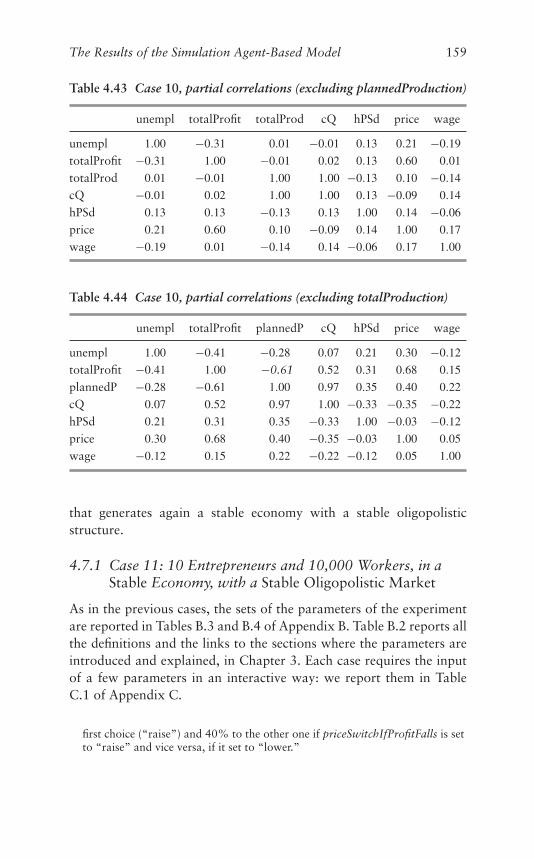
The Results of the Simulation Agent-Based Model 159
Table 4.43 Case 10, partial correlations (excluding plannedProduction)
unempl totalProfit totalProd cQ hPSd price wage
unempl 1.00 −0.31 0.01 −0.01 0.13 0.21 −0.19
totalProfit −0.31 1.00 −0.01 0.02 0.13 0.60 0.01
totalProd 0.01 −0.01 1.00 1.00 −0.13 0.10 −0.14
cQ −0.01 0.02 1.00 1.00 0.13 −0.09 0.14
hPSd 0.13 0.13 −0.13 0.13 1.00 0.14 −0.06
price 0.21 0.60 0.10 −0.09 0.14 1.00 0.17
wage −0.19 0.01 −0.14 0.14 −0.06 0.17 1.00
Table 4.44 Case 10, partial correlations (excluding totalProduction)
unempl totalProfit plannedP cQ hPSd price wage
unempl 1.00 −0.41 −0.28 0.07 0.21 0.30 −0.12
totalProfit −0.41 1.00 −0.61 0.52 0.31 0.68 0.15
plannedP −0.28 −0.61 1.00 0.97 0.35 0.40 0.22
cQ 0.07 0.52 0.97 1.00 −0.33 −0.35 −0.22
hPSd 0.21 0.31 0.35 −0.33 1.00 −0.03 −0.12
price 0.30 0.68 0.40 −0.35 −0.03 1.00 0.05
wage −0.12 0.15 0.22 −0.22 −0.12 0.05 1.00
that generates again a stable economy with a stable oligopolisticstructure.
4.7.1 Case 11: 10 Entrepreneurs and 10,000 Workers, in aStable Economy, with a Stable Oligopolistic Market
As in the previous cases, the sets of the parameters of the experimentare reported in Tables B.3 and B.4 of Appendix B. Table B.2 reports allthe definitions and the links to the sections where the parameters areintroduced and explained, in Chapter 3. Each case requires the inputof a few parameters in an interactive way: we report them in TableC.1 of Appendix C.
first choice (“raise”) and 40% to the other one if priceSwitchIfProfitFalls is setto “raise” and vice versa, if it set to “lower.”
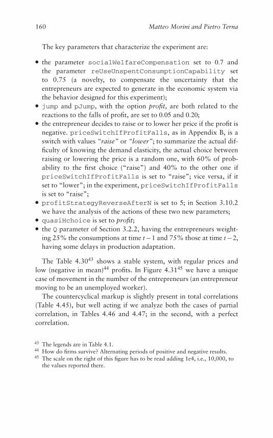
160 Matteo Morini and Pietro Terna
The key parameters that characterize the experiment are:
● the parameter socialWelfareCompensation set to 0.7 andthe parameter reUseUnspentConsumptionCapability setto 0.75 (a novelty, to compensate the uncertainty that theentrepreneurs are expected to generate in the economic system viathe behavior designed for this experiment);
● jump and pJump, with the option profit, are both related to thereactions to the falls of profit, are set to 0.05 and 0.20;
● the entrepreneur decides to raise or to lower her price if the profit isnegative. priceSwitchIfProfitFalls, as in Appendix B, is aswitch with values “raise” or “lower”; to summarize the actual dif-ficulty of knowing the demand elasticity, the actual choice betweenraising or lowering the price is a random one, with 60% of prob-ability to the first choice (“raise”) and 40% to the other one ifpriceSwitchIfProfitFalls is set to “raise”; vice versa, if itset to “lower”; in the experiment, priceSwitchIfProfitFallsis set to “raise”;
● profitStrategyReverseAfterN is set to 5; in Section 3.10.2we have the analysis of the actions of these two new parameters;
● quasiHchoice is set to profit;● the Q parameter of Section 3.2.2, having the entrepreneurs weight-
ing 25% the consumptions at time t −1 and 75% those at time t −2,having some delays in production adaptation.
The Table 4.3043 shows a stable system, with regular prices andlow (negative in mean)44 profits. In Figure 4.3145 we have a uniquecase of movement in the number of the entrepreneurs (an entrepreneurmoving to be an unemployed worker).
The countercyclical markup is slightly present in total correlations(Table 4.45), but well acting if we analyze both the cases of partialcorrelation, in Tables 4.46 and 4.47; in the second, with a perfectcorrelation.
43 The legends are in Table 4.1.44 How do firms survive? Alternating periods of positive and negative results.45 The scale on the right of this figure has to be read adding 1e4, i.e., 10,000, to
the values reported there.
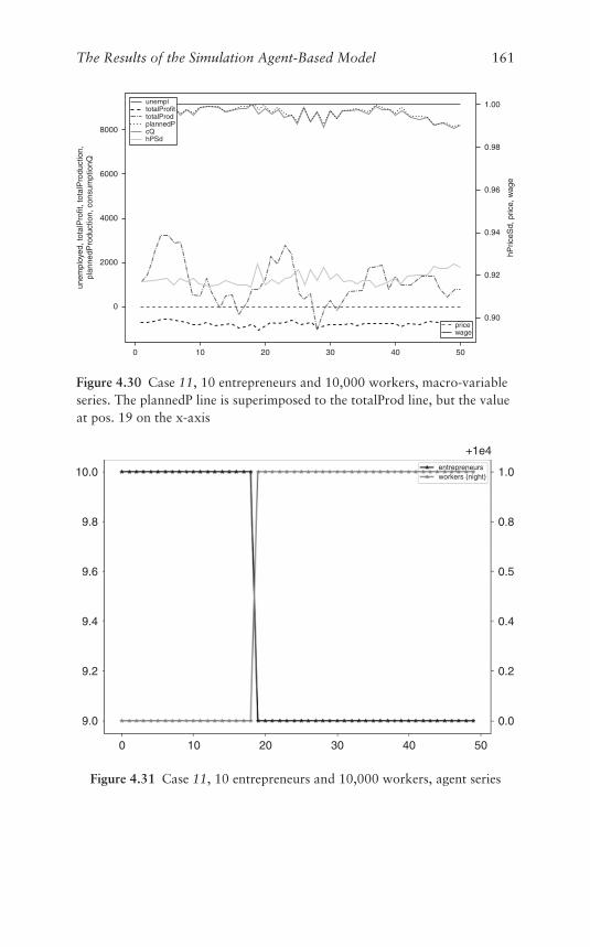
The Results of the Simulation Agent-Based Model 161
8000
6000
4000
2000
10 40 50
0.92
0.94
0.96
1.00
0.98
0.90
30200
0
hPric
eSd,
pric
e, w
age
unem
ploy
ed, t
otal
Pro
fit, t
otal
Pro
duct
ion,
plan
nedP
rodu
ctio
n, c
onsu
mpt
ionQ
unempltotalProfittotalProdplannedPcQ
wageprice
hPSd
Figure 4.30 Case 11, 10 entrepreneurs and 10,000 workers, macro-variableseries. The plannedP line is superimposed to the totalProd line, but the valueat pos. 19 on the x-axis
10.0
9.8
9.6
9.4
9.2
9.0
0 10 20 30 40 50
0.0
0.2
0.4
0.5
0.8
1.0
+1e4entrepreneursworkers (night)
Figure 4.31 Case 11, 10 entrepreneurs and 10,000 workers, agent series
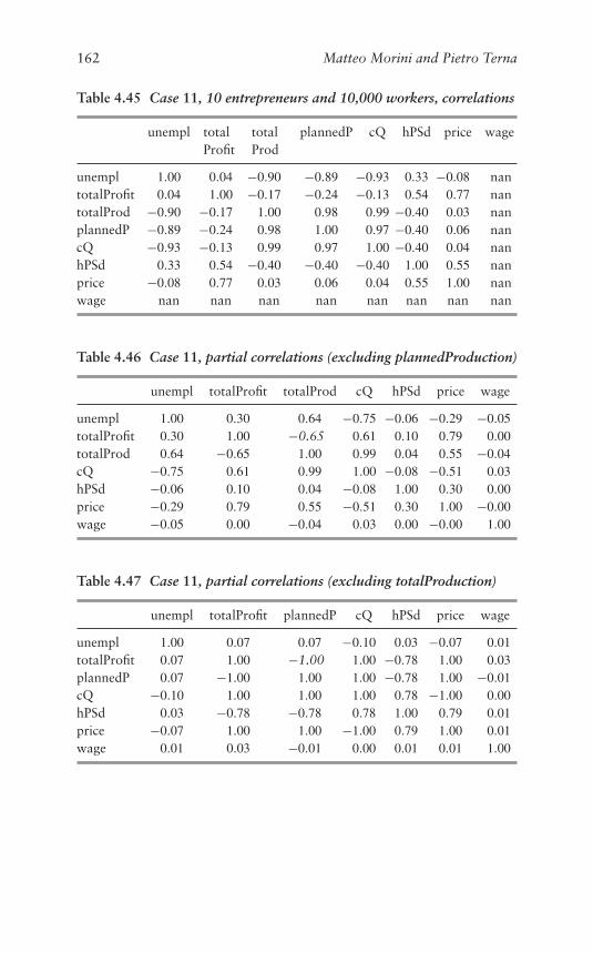
162 Matteo Morini and Pietro Terna
Table 4.45 Case 11, 10 entrepreneurs and 10,000 workers, correlations
unempl totalProfit
totalProd
plannedP cQ hPSd price wage
unempl 1.00 0.04 −0.90 −0.89 −0.93 0.33 −0.08 nantotalProfit 0.04 1.00 −0.17 −0.24 −0.13 0.54 0.77 nantotalProd −0.90 −0.17 1.00 0.98 0.99 −0.40 0.03 nanplannedP −0.89 −0.24 0.98 1.00 0.97 −0.40 0.06 nancQ −0.93 −0.13 0.99 0.97 1.00 −0.40 0.04 nanhPSd 0.33 0.54 −0.40 −0.40 −0.40 1.00 0.55 nanprice −0.08 0.77 0.03 0.06 0.04 0.55 1.00 nanwage nan nan nan nan nan nan nan nan
Table 4.46 Case 11, partial correlations (excluding plannedProduction)
unempl totalProfit totalProd cQ hPSd price wage
unempl 1.00 0.30 0.64 −0.75 −0.06 −0.29 −0.05totalProfit 0.30 1.00 −0.65 0.61 0.10 0.79 0.00totalProd 0.64 −0.65 1.00 0.99 0.04 0.55 −0.04cQ −0.75 0.61 0.99 1.00 −0.08 −0.51 0.03hPSd −0.06 0.10 0.04 −0.08 1.00 0.30 0.00price −0.29 0.79 0.55 −0.51 0.30 1.00 −0.00wage −0.05 0.00 −0.04 0.03 0.00 −0.00 1.00
Table 4.47 Case 11, partial correlations (excluding totalProduction)
unempl totalProfit plannedP cQ hPSd price wage
unempl 1.00 0.07 0.07 −0.10 0.03 −0.07 0.01totalProfit 0.07 1.00 −1.00 1.00 −0.78 1.00 0.03plannedP 0.07 −1.00 1.00 1.00 −0.78 1.00 −0.01cQ −0.10 1.00 1.00 1.00 0.78 −1.00 0.00hPSd 0.03 −0.78 −0.78 0.78 1.00 0.79 0.01price −0.07 1.00 1.00 −1.00 0.79 1.00 0.01wage 0.01 0.03 −0.01 0.00 0.01 0.01 1.00

The Results of the Simulation Agent-Based Model 163
4.8 Synopsis of Cases from 7 to 11, in the ASHAM Economy
Table 4.48 summarizes the experiments use to explore the ASHAMeconomics, looking at the results in the perspective both of emergenceof the countercyclical markup and of the changes in the structure ofthe market.
Let us briefly comment:
● the emergence of the countercyclical markup is here nearly aconstant, but in the case of the always declining economy, con-firming the relevance of the ASHAM construction as a realisticrepresentation of an economic system;
● the case 8, with the households/workers acting in a wise way, recov-ering or transferring to other people their unspent consumptioncapability, in presence of social welfare compensations quite high,produces a movement of the structure of the market toward itsopenness.
● the dynamic of the market structure in cases 9 and 9b shows animportant novelty, with the emergence of tight oligopolistic struc-tures in stable or declining economies, if the entrepreneurs payattention to the price corrections in presence/absence of unsoldproducts.
4.9 Random Values On and Off, a Test in the ASHAMEnvironment
The Oligopoly simulation project, built for the SLAPP shell, allows usto specify experiment with the random values used to generate someof its internal values.
We run again the case 8 of Section 4.4.2, with name 8modPars,modifying three of the random values in the middle of the simulation:when t = 26, we stop them with 0 as maximum value.
We use the special action feature of SLAPP, described in its Ref-erence Handbook46 (use the index to find it). This feature can beprogrammed in different ways.
If the file observerActions.txt (the file is in the main folderof the simulation project; see Section C.1 in Appendix C) contains
46 Online at https://terna.github.io/SLAPP/ .
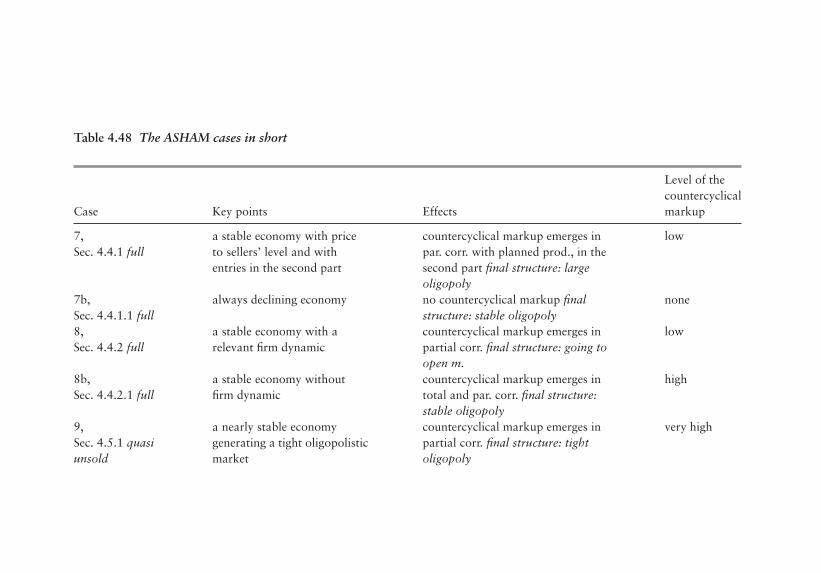
Table 4.48 The ASHAM cases in short
Level of thecountercyclical
Case Key points Effects markup
7,Sec. 4.4.1 full
a stable economy with priceto sellers’ level and withentries in the second part
countercyclical markup emerges inpar. corr. with planned prod., in thesecond part final structure: largeoligopoly
low
7b,Sec. 4.4.1.1 full
always declining economy no countercyclical markup finalstructure: stable oligopoly
none
8,Sec. 4.4.2 full
a stable economy with arelevant firm dynamic
countercyclical markup emerges inpartial corr. final structure: going toopen m.
low
8b,Sec. 4.4.2.1 full
a stable economy withoutfirm dynamic
countercyclical markup emerges intotal and par. corr. final structure:stable oligopoly
high
9,Sec. 4.5.1 quasiunsold
a nearly stable economygenerating a tight oligopolisticmarket
countercyclical markup emerges inpartial corr. final structure: tightoligopoly
very high
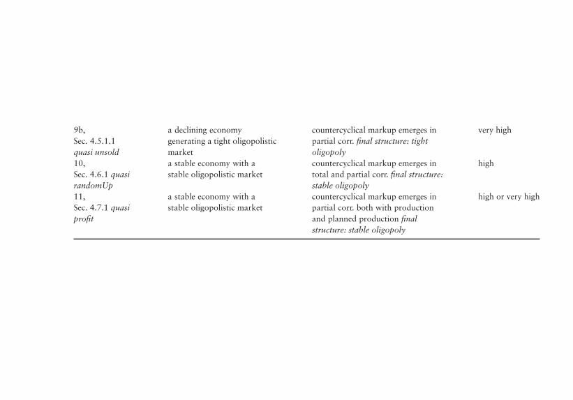
9b,Sec. 4.5.1.1quasi unsold
a declining economygenerating a tight oligopolisticmarket
countercyclical markup emerges inpartial corr. final structure: tightoligopoly
very high
10,Sec. 4.6.1 quasirandomUp
a stable economy with astable oligopolistic market
countercyclical markup emerges intotal and partial corr. final structure:stable oligopoly
high
11,Sec. 4.7.1 quasiprofit
a stable economy with astable oligopolistic market
countercyclical markup emerges inpartial corr. both with productionand planned production finalstructure: stable oligopoly
high or very high
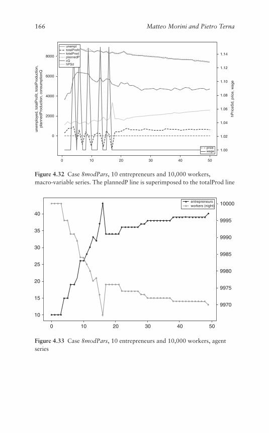
166 Matteo Morini and Pietro Terna
8000
6000
4000
2000
0
unem
ploy
ed, t
otal
Pro
fit, t
otal
Pro
duct
ion,
plan
nedP
rodu
ctio
n, c
onsu
mpt
ionQ
10 40 50
1.04
1.08
1.10
1.12
1.14
1.06
1.02
1.00
30200
hPric
eSd,
pric
e, w
age
unempltotalProfittotalProdplannedPcQ
wageprice
hPSd
Figure 4.32 Case 8modPars, 10 entrepreneurs and 10,000 workers,macro-variable series. The plannedP line is superimposed to the totalProd line
40
35
30
25
20
15
10
0 10 20 30 40 50
9970
9975
9980
9985
9990
9995
10000entrepreneursworkers (night)
Figure 4.33 Case 8modPars, 10 entrepreneurs and 10,000 workers, agentseries

The Results of the Simulation Agent-Based Model 167
the item specialAction, the simulator looks for a file with namemodPars.txt, reporting the internal names of the variables used asparameters in the model; each name followed by a new value.47
The program automatically produces the following output and thenwaits for our reply (“26” in this case):
The special action has to be activated at cycle ...-1 if never
In this example, the file modPars.txt contains:
consumptionRandomComponentSD 0randomComponentOfPlannedProduction 0maxDemandRelativeRandomShock 0
Comparing the new Figures 4.32 and 4.33 with the original Figures4.21 and 4.22, we can verify that the trends are the same, but theoriginal representations are interestingly more dynamic.
47 In the oligopoly folder, we have an example of modPars.txt file and also a filenamed observerActions with specialAction.txt that we can rename asobserverActions.txt; the original observerActions.txt can be saved withanother name or simply deleted; the recovery is from the files observerActionsno pause.txt or observerActions with pause.txt.
5 The Model Facing Empirical Data
SIMONE LOMBARDINI
In this chapter we compare the implications of our theoretical modeland simulations with the empirical data. In particular, we look at thenumber of new firms and failed ones over the business cycle. For thispurpose, we consider two time series of the number of births/deathsin the industrial sector provided by the Bureau of Labor Statistics.1
These data refer to the US economy. We have a quarterly time series,starting from March 1993.
In Figure 5.1, the hyphened line is normally far below the continu-ous one. This is consistent with the fact that US GDP has generallygrown over the period examined, except for quarters in the heavyrecession beginning in 2008. It is possible to see that when the dot-com bubble broke out, the number of enterprises born was equal tothat of the failed. The worst situation took place from the end of 2007until 2009, when the number of failed businesses was higher than thatof newborn businesses.
It is possible to recognize three cycles since 1993: the first one goesfrom 1993 to 2001, the second one from 2001 to 2007, and then asmall cycle from 2009 to 2014, where the economic growth is moreunstable. Around June 2013, the number of failed enterprises nearlyreached that of newborn businesses.
Figure 5.2 shows the ratio between newborn and failed enterprises.The dashed line at level 1 allows us to identify the economic cycles.When the continuous line is above the dashed one, the US economyis growing, and thus the number of enterprises born is far biggerthen the dead. The three previously defined business cycles are clearly
1 Entrepreneurship and the U.S. Economy, Business Employment Dynamics,Bureau of Labor Statistics, April 28, 2016. Chart 5: https://www.bls.gov/bdm/entrepreneurship/bdm_chart5.htm .
168
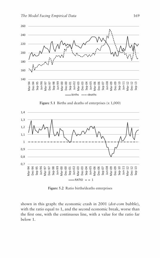
The Model Facing Empirical Data 169
Figure 5.1 Births and deaths of enterprises (x 1,000)
Figure 5.2 Ratio births/deaths enterprises
shown in this graph: the economic crash in 2001 (dot-com bubble),with the ratio equal to 1, and the second economic break, worse thanthe first one, with the continuous line, with a value for the ratio farbelow 1.
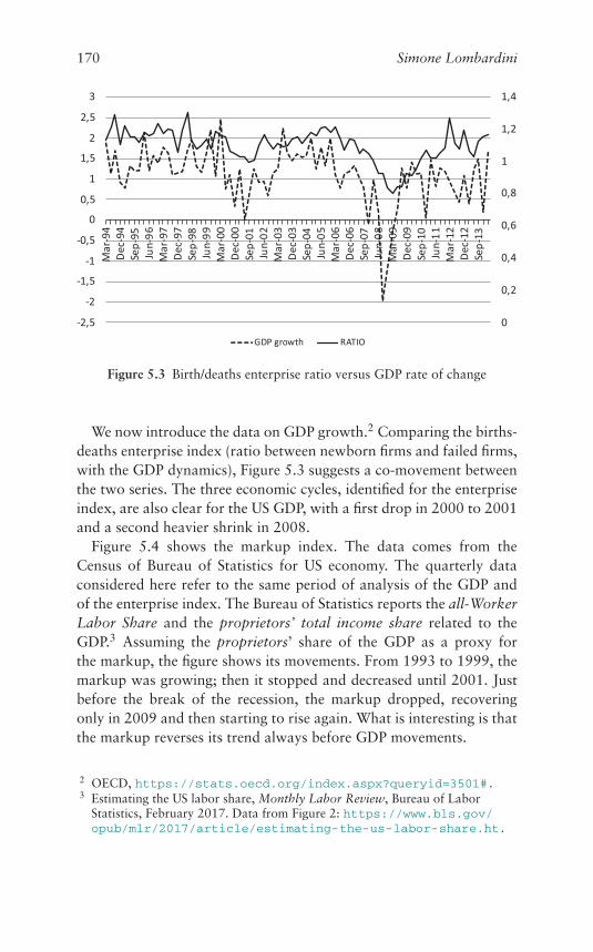
170 Simone Lombardini
Figure 5.3 Birth/deaths enterprise ratio versus GDP rate of change
We now introduce the data on GDP growth.2 Comparing the births-deaths enterprise index (ratio between newborn firms and failed firms,with the GDP dynamics), Figure 5.3 suggests a co-movement betweenthe two series. The three economic cycles, identified for the enterpriseindex, are also clear for the US GDP, with a first drop in 2000 to 2001and a second heavier shrink in 2008.
Figure 5.4 shows the markup index. The data comes from theCensus of Bureau of Statistics for US economy. The quarterly dataconsidered here refer to the same period of analysis of the GDP andof the enterprise index. The Bureau of Statistics reports the all-WorkerLabor Share and the proprietors’ total income share related to theGDP.3 Assuming the proprietors’ share of the GDP as a proxy forthe markup, the figure shows its movements. From 1993 to 1999, themarkup was growing; then it stopped and decreased until 2001. Justbefore the break of the recession, the markup dropped, recoveringonly in 2009 and then starting to rise again. What is interesting is thatthe markup reverses its trend always before GDP movements.
2 OECD, https://stats.oecd.org/index.aspx?queryid=3501# .3 Estimating the US labor share, Monthly Labor Review, Bureau of Labor
Statistics, February 2017. Data from Figure 2: https://www.bls.gov/opub/mlr/2017/article/estimating-the-us-labor-share.ht .
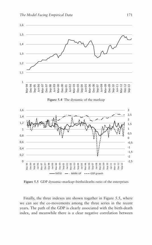
The Model Facing Empirical Data 171
Figure 5.4 The dynamic of the markup
Figure 5.5 GDP dynamic–markup–births/deaths ratio of the enterprises
Finally, the three indexes are shown together in Figure 5.5, wherewe can see the co-movements among the three series in the recentyears. The path of the GDP is clearly associated with the birth-deathindex, and meanwhile there is a clear negative correlation between
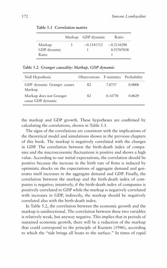
172 Simone Lombardini
Table 5.1 Correlation matrix
Markup GDP dynamic Ratio
Markup 1 −0.1341712 −0.2116298GDP dynamic 1 0.53767038Ratio 1
Table 5.2 Granger causality: Markup, GDP dynamic
Null Hypothesis Observations F-statistics Probability
GDP dynamic Granger causesMarkup
82 7.8737 0.0008
Markup does not Grangercause GDP dynamic
82 0.14778 0.8629
the markup and GDP growth. These hypotheses are confirmed bycalculating the correlations, shown in Table 5.1.
The signs of the correlations are consistent with the implications ofthe theoretical model and simulations shown in the previous chaptersof this book. The markup is negatively correlated with the changesin GDP. The correlation between the birth-death index of compa-nies and the macroeconomic fluctuations is positive and shows a highvalue. According to our initial expectations, the correlation should bepositive because the increase in the birth rate of firms is induced byoptimistic shocks on the expectations of aggregate demand and gen-erates itself increases in the aggregate demand and GDP. Finally, thecorrelation between the markup and the birth-death index of com-panies is negative; intuitively, if the birth-death index of companies ispositively correlated to GDP while the markup is negatively correlatedwith increases in GDP, indirectly, the markup should be negativelycorrelated also with the birth-death index.
In Table 5.2, the correlation between the economic growth and themarkup is unidirectional. The correlation between these two variablesis relatively weak, but anyway negative. This implies that in periods ofsustained economic growth, there will be a reduction of the markupthat could correspond to the principle of Kuznets (1946), accordingto which the “tide brings all boats to the surface.” In times of rapid
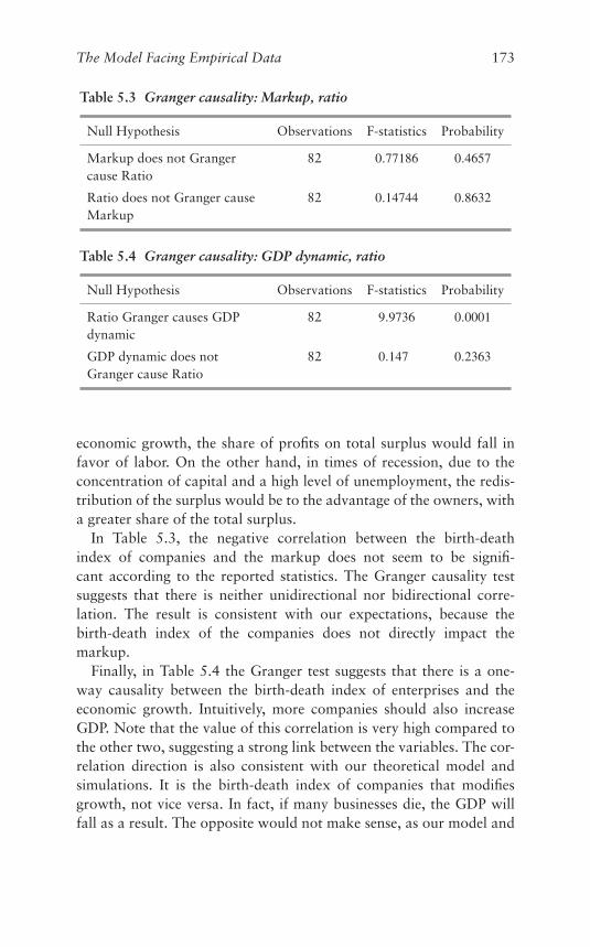
The Model Facing Empirical Data 173
Table 5.3 Granger causality: Markup, ratio
Null Hypothesis Observations F-statistics Probability
Markup does not Grangercause Ratio
82 0.77186 0.4657
Ratio does not Granger causeMarkup
82 0.14744 0.8632
Table 5.4 Granger causality: GDP dynamic, ratio
Null Hypothesis Observations F-statistics Probability
Ratio Granger causes GDPdynamic
82 9.9736 0.0001
GDP dynamic does notGranger cause Ratio
82 0.147 0.2363
economic growth, the share of profits on total surplus would fall infavor of labor. On the other hand, in times of recession, due to theconcentration of capital and a high level of unemployment, the redis-tribution of the surplus would be to the advantage of the owners, witha greater share of the total surplus.
In Table 5.3, the negative correlation between the birth-deathindex of companies and the markup does not seem to be signifi-cant according to the reported statistics. The Granger causality testsuggests that there is neither unidirectional nor bidirectional corre-lation. The result is consistent with our expectations, because thebirth-death index of the companies does not directly impact themarkup.
Finally, in Table 5.4 the Granger test suggests that there is a one-way causality between the birth-death index of enterprises and theeconomic growth. Intuitively, more companies should also increaseGDP. Note that the value of this correlation is very high compared tothe other two, suggesting a strong link between the variables. The cor-relation direction is also consistent with our theoretical model andsimulations. It is the birth-death index of companies that modifiesgrowth, not vice versa. In fact, if many businesses die, the GDP willfall as a result. The opposite would not make sense, as our model and
174 Simone Lombardini
simulations predict, by focusing on the impact of entry and exit on thedetermination of the GDP.
The data shown in the last table are consistent with the hypothesesof the model described in the book. The probability of entry, for thefirms, would be determined by the idiosyncratic information shocksfollowing equation (2.30) of Chapter 2:
Pr(entry)t =nt (1−ht )∫
0
(Pr(wt < Et−1,i (t ))i di
These shocks depend on the variance of expectations Et−1,i (t ),which is the probability that the wage is set at a lower level thanthe expected present discounted value of the future profits as anentrepreneur in case of entry. This expectation, in its turn, is stronglylinked to the “shift parameter” �t of aggregate demand in equation(2.21) of Chapter 2:
�t =∞∑
i=0
E[nt+i (Wt+i +hint+i E(�in
t+i )+het+i E(�e
t+i ))][1+E(rt+i )]i
The variance of shift parameter � is therefore dependent on futuremonetary policy expectations (the denominator), on inflation (sincethe variables in square brackets are expressed in nominal values),wages, and profit expectations (both of new entrants and incumbents),since their value appears inside the square brackets in the numerator.So, our model suggests that there should be a link among nominal val-ues of wages, profit, and interest rate, and the entry/exit of enterprises.In our model, the parameter � influences the number of entrepreneursdirectly, according to equation (2.36) of Chapter 2:
Ht = Ht−1[Pr(�in ≥ 0)] + (nt−1 − Ht−1)β(var(�t ))−− ξ(1 + ι)(1 + rt−1)FR(nt−2 − Ht−2)β(var(�t−1))
The Granger causality test shows evidence of causation from GDPchanges to births/deaths enterprises. This means that GDP trend (i.e.,the total sum of profits and wages) influences the expectation aboutfuture GDP, and in its turn, the entry decisions. Shocks on the realGDP, i.e., on the sum of profits and wages, influences births/deathsfirm as described in these equations of our model.
Furthermore, it is interesting to point out that the US data onmarkup show a countercyclical behavior. The current literature in this
The Model Facing Empirical Data 175
regard is rather mixed; however, we have calculated a simple corre-lation index. In order to verify this hypothesis, we have consideredthe same time series of Figure 5.1, cut off by 1997. From 1993 to1997, the births-deaths index for the firms is lower than in the fol-lowing years, and the correlation index for that period is positive(0, 1528).
Conclusions
Even in economics, research is meant to answer one or more questionsabout individuals’ behavior. The question we have dealt with and – webelieve – answered with this book is the following.
Do entry, exit, and strategic interactions among oligopolists and changes inmarket structure affect the macroeconomy?
In this book we introduce a new approach in macroeconomics wheremarket structure is endogenous, its changes generate macroeconomicfluctuations, and its configuration is, in its turn, affected by the natureand features of the macroeconomic equilibrium. In particular, the the-oretical chapter of our book provides a modeling framework, thatplug oligopolistic firms’ strategic interactions in a macromodel mayalso allow us to keep track of social mobility and income distribution.
Since the focus of our theoretical framework is on the subjectivedecisions of interactive agents, a logical consequence of this assump-tion is choosing a methodology for simulations that is founded onthe premises of realistically modeling the actual behavior of individualagents.
The agent-based modeling (ABM) technique has its starting pointin populations of agents, representing individuals or more generallyentities. From there, we construct our models via computer code oper-ating in dedicated software environments, with each agent representedby a component of the whole code. As in the Introduction, we under-line that an ABM does not introduce equations governing the effectsof the agents’ behavior at the macro level, but it allows us to observethe emergence of those effects, e.g., analyzing individual and globaloutcomes generated by the agents’ actions.
Thanks to ABMs, we can manage boundedly rational behavior andnon-equilibrium dynamics.
An interesting implication of our theoretical analysis and simu-lations is the fact that expansions are, in general, associated with
176
Conclusions 177
social mobility, which is generated by entry and higher birth of newfirms compared to failed companies. In this sense, our work canalso be interpreted as a theory of social mobility over the businesscycle.
A SummaryWe now briefly summarize the main achievements of the differentchapters of this book.
In Chapter 1, we explored the premises of the whole work, includ-ing the theoretical pillars of the relationships between the industrialstructure and the macroeconomy.
In Chapter 2, the algebraic framework of a new macro-model isanalytically dissected, to prepare a sound basis for the experiments insimulation.
In Chapter 3, starting from the model outline reported in Figure3.1, we developed a detailed description of the steps the simulationundertakes over its course with the actions of the different kinds ofagents.
In Chapter 4 we discovered the results emerging from the simu-lation experiments, in the perspective both of the presence of thecountercyclical markup phenomenon and of the different marketstructures generated by the simulation.
In Chapter 5 we examined some actual data related to the GDPcycle and to the income components, observing a significant presenceof the countercyclical markup.
Appendix A produces a key explanation about the way a decentral-ized market based on agents actually works. Those pages are worthyto be read also independently from the other parts of the book.
In Appendix B we report the collection of the parameters (namesand values) used in this book.
In Appendix C we offer the technical details useful for repeating theexperiments of the book or developing new ones.
Future ResearchWe hope that the theoretical framework of this book may be a use-ful tool for further research and extensions, where the endogeneity ofmarket structure in a macromodel and its potential implications areanalyzed in their macroeconomic implications.

178 Conclusions
An interesting development for future research could deal withthe macroeconomic implications of the interactions between increas-ing/decreasing returns to scale, with respect to capital, variable barri-ers to entry, and market structure, i.e., a richer and more extendedformalization of the way firms’ technology interacts with capital,capital markets, and the macroeconomy.
We trust that our framework could be used for a new kind of policyanalyses, based on the link among entry of new firms, social mobilityand economic expansions. We do hope that this little and modest pro-posal may be of some help to the work of other colleagues and felloweconomists.
Appendices

Appendix A
The Structure of an AtomisticSimplified Hayekian Market
MATTEO MORINI AND PIETRO TERNA
We propose a simplified version of the Hayek’s decentralized markethypothesis, considering elementary processes of price adaptation inexchanges.
As a theoretical framework, we refer to the paper of Bowles et al.(2017).
Section A.1 reports the structure of the model and its warming upphase. In Section A.2 we introduce an elementary agent-based modelof a market, with emergent (quite interesting) price dynamics.
A counter-example is also introduced in Section A.3, showing that –with tiny modification – we generate implausible price dynamics.
In Section A.4 we report some technical analyses of the cases withunmatching numbers of buyers and sellers. These analyses are stronglyrelated to the ratio between sellers and buyers in Sections 3.6 and 3.7.
In Section A.5 we deepen the problem of the agents that seem tobe idle, having the level of their reservation price too low to buy. Theanalysis is relevant to increase the number of sub-steps in the phasesof market interaction, as described in Section 3.7.
Codes and sources:
● The simulation generating the Figures A.1 to A.19 are run usingdemandOfferCurvesBW2.ipynb.
● All the material of this Appendix is online athttps://terna.github.io/microHayekianMarket/ .
A.1 The Structure of the Model and the Warming Up Phase
Our agents are simply prices (a number, the price, represents the agentin the agent vector), to be interpreted as reservation prices.1
1 The max price a buyer could pay and the min one a seller could accept are keptreserved, i.e., not declared.
181
182 Matteo Morini and Pietro Terna
The agents act over the time that we organize in cycles; within acycle, all the buyers act once, in random order.
We have two price vectors: pLb with item pLbi for the buyers, and
pLs with item pLsj for the sellers. The i th or the j th elements of the
vectors are prices, which we use here also as agents.Both in the simplified Hayekian perspective (Section A.2) and in
the unstructured one (Section A.3), we have to pre-run a warning upaction.
With the warming up phase, we define:
● d0 – the lower bound of the random uniform numbers, both for thebuyers and the sellers, in the warming up phase;
in the running phase, the lower bound is 0;● d1 – the upper bound of the random uniform numbers for the
buyers;● d2 – the upper bound of the random uniform numbers for the sellers;● nCycles – number of simulation cycles;● nBuyers – number of the buyers;● nSellers – number of the sellers;● seed – the seed of the random numbers;● the initial buyer i reservation price, different for each buyer: pb,i =
11+ui
with ui ∼ U(d0, d1);● the initial seller j reservation price, different for each seller: ps, j =
1 + u j with u j ∼ U(d0, d2);● buyersSellers Ratio – the ratio nBuyers
nSellers ;● sellers Buyers Ratio – the ratio nSellers
nBuyers ;● usingRatios – a logic variable activating limitations to d1 or d2● squeezeRate – always < 1, as further compression of d1 or d2● usingSqueezeRate – a logic variable to further squeeze d1 or d2
With d0 = 0.1, d1 = 0.2, d2 = 0.2, sorting in decreasing orderthe vector pLb and in increasing order the vector pLs , we obtain inFigure A.1 two not overlapping price sequences that we can interpretas a demand curve (black) and an offer one (gray), but actually arebuyers’ price and sellers’ price curves.
A.2 The Atomistic Hayekian Version
The buyers and the sellers meet randomly. Buyer i and seller jexchange if pLb
i ≥ pLsj ; the deal is recorded at the price of the seller
pLsj .
2
2 In the mall, sell prices are public.
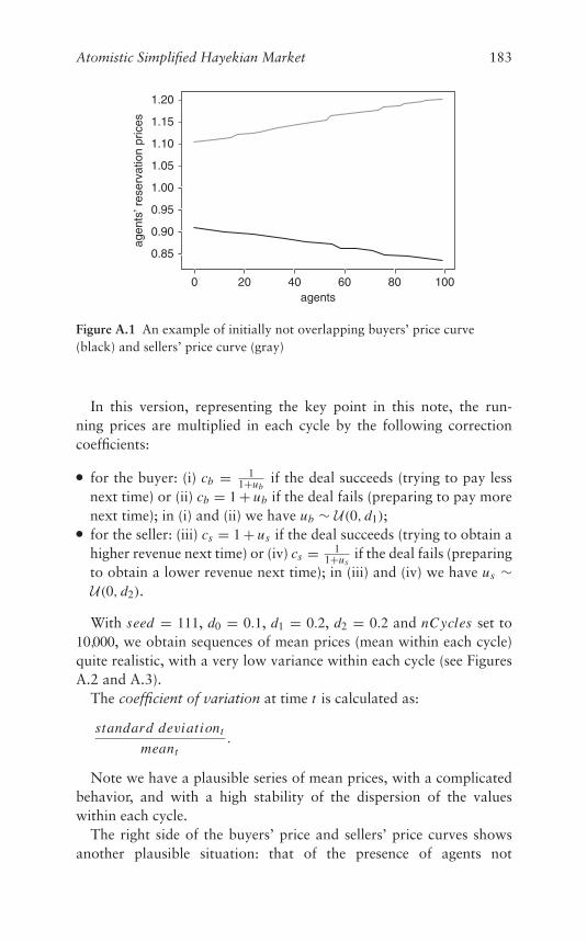
Atomistic Simplified Hayekian Market 183
1.20
1.15
1.10
1.05
1.00
agen
ts’ r
eser
vatio
n pr
ices
0.95
0.90
0.85
0 1008060agents
4020
Figure A.1 An example of initially not overlapping buyers’ price curve(black) and sellers’ price curve (gray)
In this version, representing the key point in this note, the run-ning prices are multiplied in each cycle by the following correctioncoefficients:
● for the buyer: (i) cb = 11+ub
if the deal succeeds (trying to pay lessnext time) or (ii) cb = 1 + ub if the deal fails (preparing to pay morenext time); in (i) and (ii) we have ub ∼ U(0, d1);
● for the seller: (iii) cs = 1 + us if the deal succeeds (trying to obtain ahigher revenue next time) or (iv) cs = 1
1+usif the deal fails (preparing
to obtain a lower revenue next time); in (iii) and (iv) we have us ∼U(0, d2).
With seed = 111, d0 = 0.1, d1 = 0.2, d2 = 0.2 and nCycles set to10,000, we obtain sequences of mean prices (mean within each cycle)quite realistic, with a very low variance within each cycle (see FiguresA.2 and A.3).
The coefficient of variation at time t is calculated as:
standard deviationt
meant.
Note we have a plausible series of mean prices, with a complicatedbehavior, and with a high stability of the dispersion of the valueswithin each cycle.
The right side of the buyers’ price and sellers’ price curves showsanother plausible situation: that of the presence of agents not
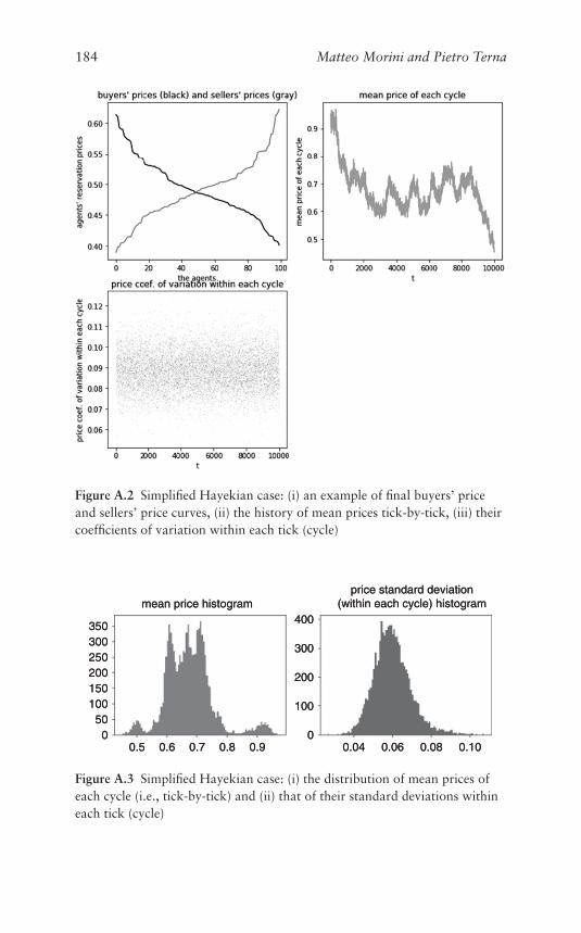
184 Matteo Morini and Pietro Terna
Figure A.2 Simplified Hayekian case: (i) an example of final buyers’ priceand sellers’ price curves, (ii) the history of mean prices tick-by-tick, (iii) theircoefficients of variation within each tick (cycle)
mean price histogrammean price histogramprice standard deviation
(within each cycle) histogramprice standard deviation
(within each cycle) histogram
350350300300250250200200150150100100505000
0.60.6 0.70.7 0.80.80.50.5 0.90.9 0.060.06 0.100.100.040.04 0.080.08
400400
300300
200200
100100
00
Figure A.3 Simplified Hayekian case: (i) the distribution of mean prices ofeach cycle (i.e., tick-by-tick) and (ii) that of their standard deviations withineach tick (cycle)
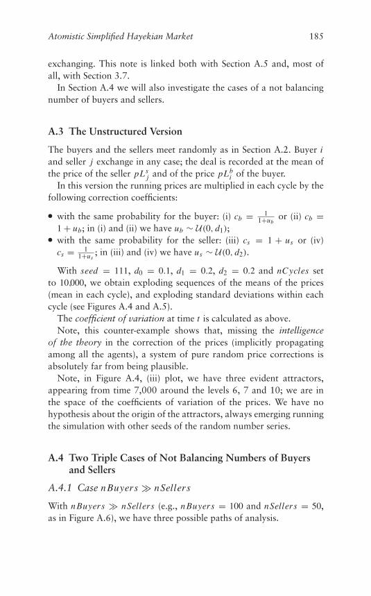
Atomistic Simplified Hayekian Market 185
exchanging. This note is linked both with Section A.5 and, most ofall, with Section 3.7.
In Section A.4 we will also investigate the cases of a not balancingnumber of buyers and sellers.
A.3 The Unstructured Version
The buyers and the sellers meet randomly as in Section A.2. Buyer iand seller j exchange in any case; the deal is recorded at the mean ofthe price of the seller pLs
j and of the price pLbi of the buyer.
In this version the running prices are multiplied in each cycle by thefollowing correction coefficients:
● with the same probability for the buyer: (i) cb = 11+ub
or (ii) cb =1 + ub; in (i) and (ii) we have ub ∼ U(0, d1);
● with the same probability for the seller: (iii) cs = 1 + us or (iv)cs = 1
1+us; in (iii) and (iv) we have us ∼ U(0, d2).
With seed = 111, d0 = 0.1, d1 = 0.2, d2 = 0.2 and nCycles setto 10,000, we obtain exploding sequences of the means of the prices(mean in each cycle), and exploding standard deviations within eachcycle (see Figures A.4 and A.5).
The coefficient of variation at time t is calculated as above.Note, this counter-example shows that, missing the intelligence
of the theory in the correction of the prices (implicitly propagatingamong all the agents), a system of pure random price corrections isabsolutely far from being plausible.
Note, in Figure A.4, (iii) plot, we have three evident attractors,appearing from time 7,000 around the levels 6, 7 and 10; we are inthe space of the coefficients of variation of the prices. We have nohypothesis about the origin of the attractors, always emerging runningthe simulation with other seeds of the random number series.
A.4 Two Triple Cases of Not Balancing Numbers of Buyersand Sellers
A.4.1 Case nBuyers � nSellers
With nBuyers � nSellers (e.g., nBuyers = 100 and nSellers = 50,as in Figure A.6), we have three possible paths of analysis.
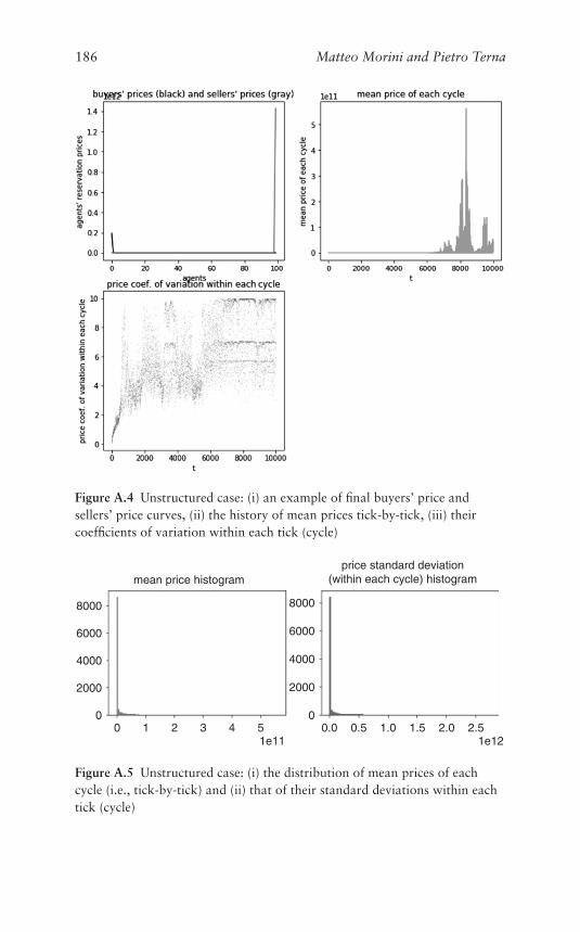
186 Matteo Morini and Pietro Terna
Figure A.4 Unstructured case: (i) an example of final buyers’ price andsellers’ price curves, (ii) the history of mean prices tick-by-tick, (iii) theircoefficients of variation within each tick (cycle)
mean price histogramprice standard deviation
(within each cycle) histogram
8000
1e114321 50
6000
4000
2000
00.5 1.0 1.5 2.00.0 2.5
1e12
8000
6000
4000
2000
0
Figure A.5 Unstructured case: (i) the distribution of mean prices of eachcycle (i.e., tick-by-tick) and (ii) that of their standard deviations within eachtick (cycle)
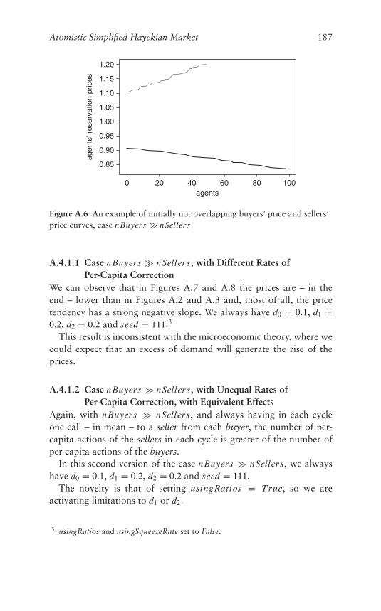
Atomistic Simplified Hayekian Market 187
1.20
1.15
1.10
1.05
1.00
0.95
0.90
0.85
0 20 40 60agents
agen
ts’ r
eser
vatio
n pr
ices
80 100
Figure A.6 An example of initially not overlapping buyers’ price and sellers’price curves, case nBuyers � nSellers
A.4.1.1 Case nBuyers � nSellers, with Different Rates ofPer-Capita Correction
We can observe that in Figures A.7 and A.8 the prices are – in theend – lower than in Figures A.2 and A.3 and, most of all, the pricetendency has a strong negative slope. We always have d0 = 0.1, d1 =0.2, d2 = 0.2 and seed = 111.3
This result is inconsistent with the microeconomic theory, where wecould expect that an excess of demand will generate the rise of theprices.
A.4.1.2 Case nBuyers � nSellers, with Unequal Rates ofPer-Capita Correction, with Equivalent Effects
Again, with nBuyers � nSellers, and always having in each cycleone call – in mean – to a seller from each buyer, the number of per-capita actions of the sellers in each cycle is greater of the number ofper-capita actions of the buyers.
In this second version of the case nBuyers � nSellers, we alwayshave d0 = 0.1, d1 = 0.2, d2 = 0.2 and seed = 111.
The novelty is that of setting usingRatios = T rue, so we areactivating limitations to d1 or d2.
3 usingRatios and usingSqueezeRate set to False.
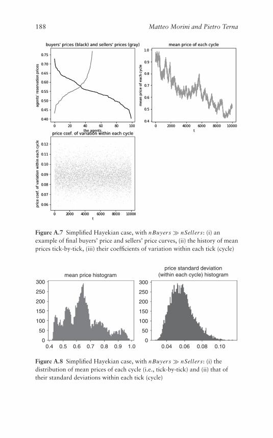
188 Matteo Morini and Pietro Terna
Figure A.7 Simplified Hayekian case, with nBuyers � nSellers: (i) anexample of final buyers’ price and sellers’ price curves, (ii) the history of meanprices tick-by-tick, (iii) their coefficients of variation within each tick (cycle)
mean price histogram300
250
200
150
100
50
00.5 0.6 0.7 0.8 0.90.4 1.0
price standard deviation(within each cycle) histogram
300
250
200
150
100
50
00.06 0.080.04 0.10
Figure A.8 Simplified Hayekian case, with nBuyers � nSellers: (i) thedistribution of mean prices of each cycle (i.e., tick-by-tick) and (ii) that oftheir standard deviations within each tick (cycle)
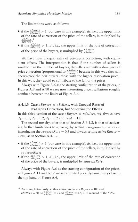
Atomistic Simplified Hayekian Market 189
The limitations work as follows:
● if the nBuyersnSellers > 1 (our case in this example), d2, i.e., the upper limit
of the rate of correction of the price of the sellers, is multiplied bynSellersnBuyers ;4
● if the nSellersnBuyers > 1, d1, i.e., the upper limit of the rate of correction
of the price of the buyers, is multiplied by nBuyersnSellers .
We have now unequal rates of per-capita correction, with equiv-alent effects. The interpretation is that if the number of sellers issmaller than the number of buyers, the sellers act with a slow pace ofprice correction (proportional to nSellers
nBuyers ) because in this way they cancherry-pick the best buyers (those with the higher reservation price).In this way, they avoid to contribute to the fall of the prices.
Always with Figure A.6 as the starting configuration of the prices, inFigures A.9 and A.10 we see now interesting price oscillations roughlyconfined between the limits of Figure A.6.
A.4.1.3 Case nBuyers � nSellers, with Unequal Rates ofPer-Capita Correction, but Squeezing the Effects
In this third version of the case nBuyers � nSellers, we always haved0 = 0.1, d1 = 0.2, d2 = 0.2 and seed = 111.
The second novelty, after that of Section A.4.1.2, is that of activat-ing further limitations to d1 or d2 by setting usingSqueeze = T rue,introducing the squeezeRate = 0.3 and always setting usingRatios =T rue, as in Section A.4.1.2:
● if the nBuyersnSellers > 1 (our case in this example), d2, i.e., the upper limit
of the rate of correction of the price of the sellers, is multiplied bysqueezeRate;
● if the nSellersnBuyers > 1, d1, i.e., the upper limit of the rate of correction
of the price of the buyers, is multiplied by squeezeRate.
Always with Figure A.6 as the starting configuration of the prices,in Figures A.11 and A.12 we see a limited price dynamic, very close tothe top band of Figure A.6.
4 An example to clarify: in this section we have nBuyers = 100 andnSellers = 50, so nBuyers
nSellers ≡ 2 and nSellersnBuyers ≡ 0.5; d2 is reduced of the 50%.
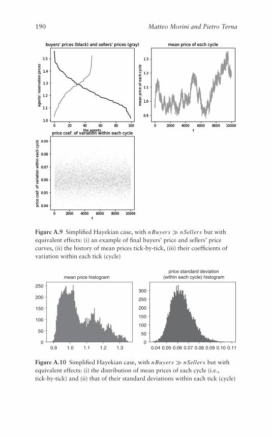
190 Matteo Morini and Pietro Terna
Figure A.9 Simplified Hayekian case, with nBuyers � nSellers but withequivalent effects: (i) an example of final buyers’ price and sellers’ pricecurves, (ii) the history of mean prices tick-by-tick, (iii) their coefficients ofvariation within each tick (cycle)
mean price histogramprice standard deviation
(within each cycle) histogram
250
200
150
100
50
01.0 1.1 1.20.9 1.3 0.05 0.06 0.07 0.08 0.09 0.100.04 0.11
300
250
200
150
100
50
0
Figure A.10 Simplified Hayekian case, with nBuyers � nSellers but withequivalent effects: (i) the distribution of mean prices of each cycle (i.e.,tick-by-tick) and (ii) that of their standard deviations within each tick (cycle)
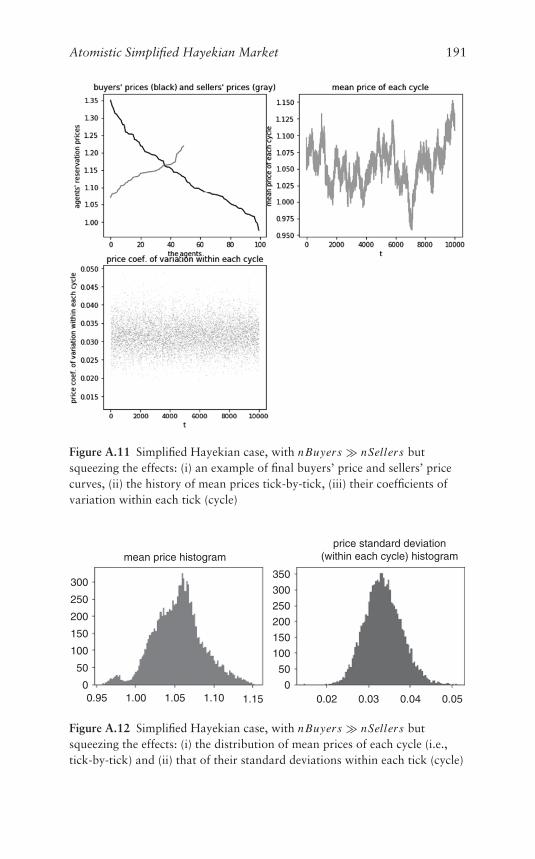
Atomistic Simplified Hayekian Market 191
Figure A.11 Simplified Hayekian case, with nBuyers � nSellers butsqueezing the effects: (i) an example of final buyers’ price and sellers’ pricecurves, (ii) the history of mean prices tick-by-tick, (iii) their coefficients ofvariation within each tick (cycle)
mean price histogram
300
250
200
150
100
50
01.101.051.00 1.150.95
price standard deviation(within each cycle) histogram
300
350
250
200
150
100
50
00.040.03 0.050.02
Figure A.12 Simplified Hayekian case, with nBuyers � nSellers butsqueezing the effects: (i) the distribution of mean prices of each cycle (i.e.,tick-by-tick) and (ii) that of their standard deviations within each tick (cycle)
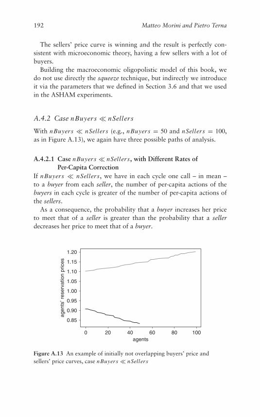
192 Matteo Morini and Pietro Terna
The sellers’ price curve is winning and the result is perfectly con-sistent with microeconomic theory, having a few sellers with a lot ofbuyers.
Building the macroeconomic oligopolistic model of this book, wedo not use directly the squeeze technique, but indirectly we introduceit via the parameters that we defined in Section 3.6 and that we usedin the ASHAM experiments.
A.4.2 Case nBuyers � nSellers
With nBuyers � nSellers (e.g., nBuyers = 50 and nSellers = 100,as in Figure A.13), we again have three possible paths of analysis.
A.4.2.1 Case nBuyers � nSellers, with Different Rates ofPer-Capita Correction
If nBuyers � nSellers, we have in each cycle one call – in mean –to a buyer from each seller, the number of per-capita actions of thebuyers in each cycle is greater of the number of per-capita actions ofthe sellers.
As a consequence, the probability that a buyer increases her priceto meet that of a seller is greater than the probability that a sellerdecreases her price to meet that of a buyer.
1.20
1.15
1.10
1.05
1.00
0.95
0.90
0.85
0 20 40 60agents
agen
ts’ r
eser
vatio
n pr
ices
80 100
Figure A.13 An example of initially not overlapping buyers’ price andsellers’ price curves, case nBuyers � nSellers
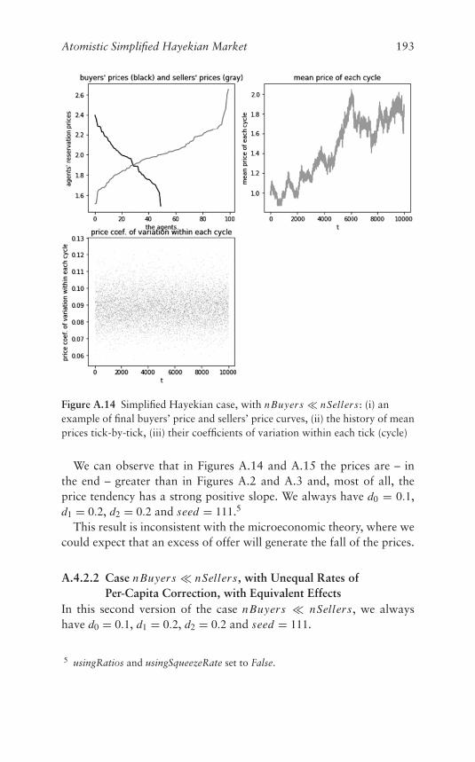
Atomistic Simplified Hayekian Market 193
Figure A.14 Simplified Hayekian case, with nBuyers � nSellers: (i) anexample of final buyers’ price and sellers’ price curves, (ii) the history of meanprices tick-by-tick, (iii) their coefficients of variation within each tick (cycle)
We can observe that in Figures A.14 and A.15 the prices are – inthe end – greater than in Figures A.2 and A.3 and, most of all, theprice tendency has a strong positive slope. We always have d0 = 0.1,d1 = 0.2, d2 = 0.2 and seed = 111.5
This result is inconsistent with the microeconomic theory, where wecould expect that an excess of offer will generate the fall of the prices.
A.4.2.2 Case nBuyers � nSellers, with Unequal Rates ofPer-Capita Correction, with Equivalent Effects
In this second version of the case nBuyers � nSellers, we alwayshave d0 = 0.1, d1 = 0.2, d2 = 0.2 and seed = 111.
5 usingRatios and usingSqueezeRate set to False.
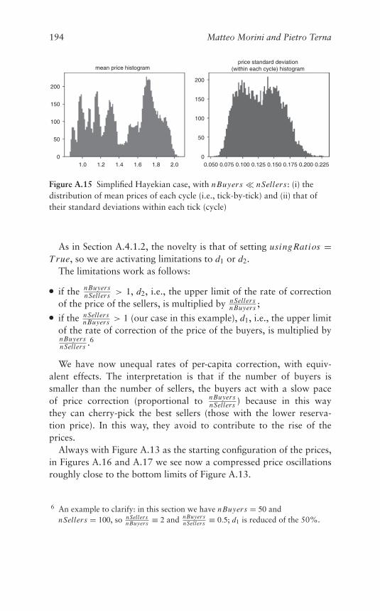
194 Matteo Morini and Pietro Terna
mean price histogramprice standard deviation
(within each cycle) histogram
200
150
100
50
01.0 1.2 1.4 1.6 1.8 2.0
200
150
100
50
00.050 0.075 0.100 0.125 0.150 0.175 0.200 0.225
Figure A.15 Simplified Hayekian case, with nBuyers � nSellers: (i) thedistribution of mean prices of each cycle (i.e., tick-by-tick) and (ii) that oftheir standard deviations within each tick (cycle)
As in Section A.4.1.2, the novelty is that of setting usingRatios =T rue, so we are activating limitations to d1 or d2.
The limitations work as follows:
● if the nBuyersnSellers > 1, d2, i.e., the upper limit of the rate of correction
of the price of the sellers, is multiplied by nSellersnBuyers ;
● if the nSellersnBuyers > 1 (our case in this example), d1, i.e., the upper limit
of the rate of correction of the price of the buyers, is multiplied bynBuyersnSellers .6
We have now unequal rates of per-capita correction, with equiv-alent effects. The interpretation is that if the number of buyers issmaller than the number of sellers, the buyers act with a slow paceof price correction (proportional to nBuyers
nSellers ) because in this waythey can cherry-pick the best sellers (those with the lower reserva-tion price). In this way, they avoid to contribute to the rise of theprices.
Always with Figure A.13 as the starting configuration of the prices,in Figures A.16 and A.17 we see now a compressed price oscillationsroughly close to the bottom limits of Figure A.13.
6 An example to clarify: in this section we have nBuyers = 50 andnSellers = 100, so nSellers
nBuyers ≡ 2 and nBuyersnSellers ≡ 0.5; d1 is reduced of the 50%.
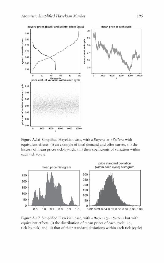
Atomistic Simplified Hayekian Market 195
Figure A.16 Simplified Hayekian case, with nBuyers � nSellers withequivalent effects: (i) an example of final demand and offer curves, (ii) thehistory of mean prices tick-by-tick, (iii) their coefficients of variation withineach tick (cycle)
mean price histogramprice standard deviation
(within each cycle) histogram
250
200
150
100
50
0
300
250
200
150
100
50
00.9 1.00.5 0.6 0.7 0.8 0.040.03 0.05 0.06 0.07 0.080.02 0.09
Figure A.17 Simplified Hayekian case, with nBuyers � nSellers but withequivalent effects: (i) the distribution of mean prices of each cycle (i.e.,tick-by-tick) and (ii) that of their standard deviations within each tick (cycle)
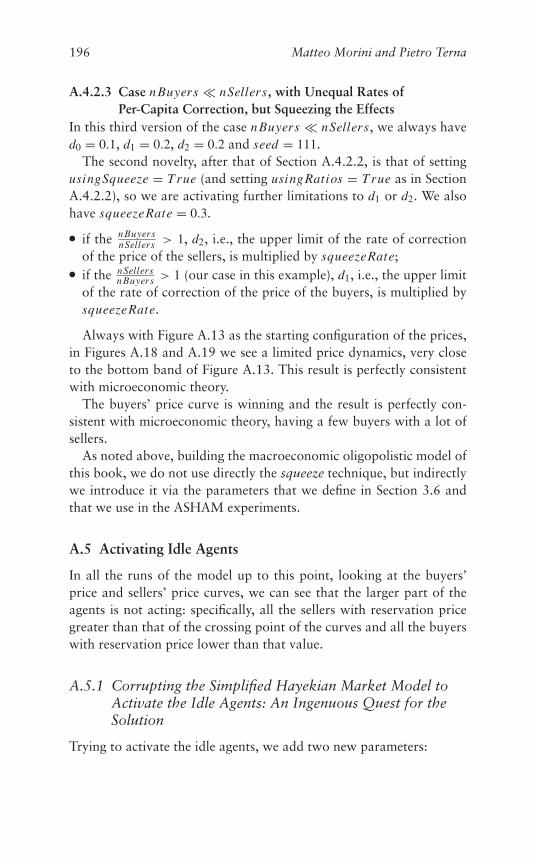
196 Matteo Morini and Pietro Terna
A.4.2.3 Case nBuyers � nSellers, with Unequal Rates ofPer-Capita Correction, but Squeezing the Effects
In this third version of the case nBuyers � nSellers, we always haved0 = 0.1, d1 = 0.2, d2 = 0.2 and seed = 111.
The second novelty, after that of Section A.4.2.2, is that of settingusingSqueeze = T rue (and setting usingRatios = T rue as in SectionA.4.2.2), so we are activating further limitations to d1 or d2. We alsohave squeezeRate = 0.3.
● if the nBuyersnSellers > 1, d2, i.e., the upper limit of the rate of correction
of the price of the sellers, is multiplied by squeezeRate;● if the nSellers
nBuyers > 1 (our case in this example), d1, i.e., the upper limitof the rate of correction of the price of the buyers, is multiplied bysqueezeRate.
Always with Figure A.13 as the starting configuration of the prices,in Figures A.18 and A.19 we see a limited price dynamics, very closeto the bottom band of Figure A.13. This result is perfectly consistentwith microeconomic theory.
The buyers’ price curve is winning and the result is perfectly con-sistent with microeconomic theory, having a few buyers with a lot ofsellers.
As noted above, building the macroeconomic oligopolistic model ofthis book, we do not use directly the squeeze technique, but indirectlywe introduce it via the parameters that we define in Section 3.6 andthat we use in the ASHAM experiments.
A.5 Activating Idle Agents
In all the runs of the model up to this point, looking at the buyers’price and sellers’ price curves, we can see that the larger part of theagents is not acting: specifically, all the sellers with reservation pricegreater than that of the crossing point of the curves and all the buyerswith reservation price lower than that value.
A.5.1 Corrupting the Simplified Hayekian Market Model toActivate the Idle Agents: An Ingenuous Quest for theSolution
Trying to activate the idle agents, we add two new parameters:
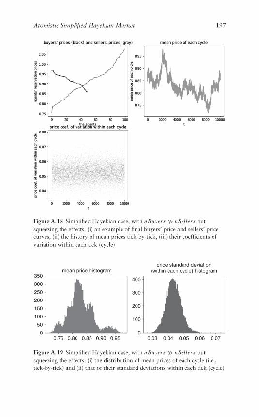
Atomistic Simplified Hayekian Market 197
Figure A.18 Simplified Hayekian case, with nBuyers � nSellers butsqueezing the effects: (i) an example of final buyers’ price and sellers’ pricecurves, (ii) the history of mean prices tick-by-tick, (iii) their coefficients ofvariation within each tick (cycle)
mean price histogramprice standard deviation
(within each cycle) histogram
250
300
350
200
150
100
50
0
300
400
200
100
00.04 0.050.03 0.070.060.950.75 0.80 0.85 0.90
Figure A.19 Simplified Hayekian case, with nBuyers � nSellers butsqueezing the effects: (i) the distribution of mean prices of each cycle (i.e.,tick-by-tick) and (ii) that of their standard deviations within each tick (cycle)
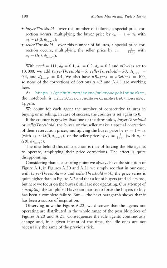
198 Matteo Morini and Pietro Terna
● buyerThreshold – over this number of failures, a special price cor-rection occurs, multiplying the buyer price by cb = 1 + ub withub ∼ U(0, d1overT );
● sellerThreshold – over this number of failures, a special price cor-rection occurs, multiplying the seller price by cs = 1
1+uswith
us ∼ U(0, d2overT ).
With seed = 111, d0 = 0.1, d1 = 0.2, d2 = 0.2 and nCycles set to10, 000, we add buyerThreshold = 5, sellerThreshold = 50, d1overT =0.4, and d2overT = 0.4. We also have nBuyers = nSellers = 100,so none of the corrections of Sections A.4.2 and A.4.1 are workinghere.
At https://github.com/terna/microHayekianMarket,the notebook is microCorruptedHayekianMarket\_baseBW.ipynb.
We count for each agent the number of consecutive failures inbuying or in selling. In case of success, the counter is set again to 0.
If the counter is greater than one of the thresholds, buyerThresholdor sellerThreshold, the buyer or the seller make a special correctionof their reservation prices, multiplying the buyer price by cb = 1 + ub
(with ub ∼ U(0, d1overT )) or the seller price by cs = 11+us
(with us ∼U(0, d2overT )).
The idea behind this construction is that of forcing the idle agentsto operate, amplifying their price corrections. The effect is quitedisappointing.
Considering that as a starting point we always have the situation ofFigure A.1, in Figures A.20 and A.21 we simply see that in our case,with buyerThreshold = 5 and sellerThreshold = 50, the price series isquite higher than in Figure A.2 and that a lot of buyers (and sellers too,but here we focus on the buyers) still are not operating. Our attempt ofcorrupting the simplified Hayekian market to force the buyers to buyhas been a complete failure. But . . . the next paragraph shows that ithas been a source of inspiration.
Observing now the Figure A.22, we discover that the agents notoperating are distributed in the whole range of the possible prices ofFigures A.20 and A.21. Consequence: the idle agents continuouslychange and, in a given instant of the time, the idle ones are notnecessarily the same of the previous tick.
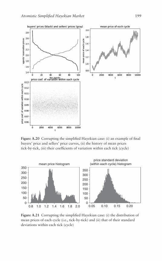
Atomistic Simplified Hayekian Market 199
Figure A.20 Corrupting the simplified Hayekian case: (i) an example of finalbuyers’ price and sellers’ price curves, (ii) the history of mean pricestick-by-tick, (iii) their coefficients of variation within each tick (cycle)
mean price histogramprice standard deviation
(within each cycle) histogram
250300350
200150100500
250
300
350
200
150
100
50
01.0 1.2 1.4 1.6 1.8 2.00.8 0.10 0.150.05 0.20
Figure A.21 Corrupting the simplified Hayekian case: (i) the distribution ofmean prices of each cycle (i.e., tick-by-tick) and (ii) that of their standarddeviations within each tick (cycle)
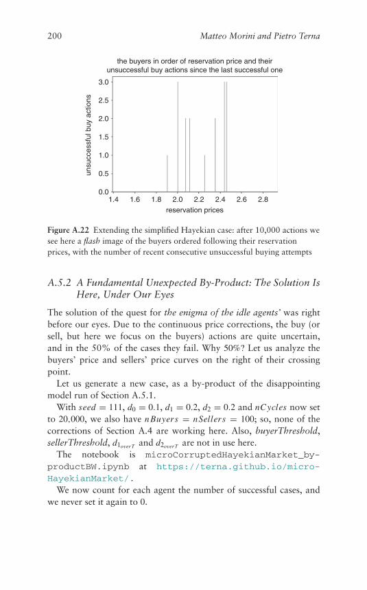
200 Matteo Morini and Pietro Terna
the buyers in order of reservation price and theirunsuccessful buy actions since the last successful one
unsu
cces
sful
buy
act
ions
3.0
2.5
2.0
1.5
1.0
0.5
0.01.4 1.6 1.8 2.0
reservation prices
2.2 2.4 2.6 2.8
Figure A.22 Extending the simplified Hayekian case: after 10,000 actions wesee here a flash image of the buyers ordered following their reservationprices, with the number of recent consecutive unsuccessful buying attempts
A.5.2 A Fundamental Unexpected By-Product: The Solution IsHere, Under Our Eyes
The solution of the quest for the enigma of the idle agents’ was rightbefore our eyes. Due to the continuous price corrections, the buy (orsell, but here we focus on the buyers) actions are quite uncertain,and in the 50% of the cases they fail. Why 50%? Let us analyze thebuyers’ price and sellers’ price curves on the right of their crossingpoint.
Let us generate a new case, as a by-product of the disappointingmodel run of Section A.5.1.
With seed = 111, d0 = 0.1, d1 = 0.2, d2 = 0.2 and nCycles now setto 20,000, we also have nBuyers = nSellers = 100; so, none of thecorrections of Section A.4 are working here. Also, buyerThreshold,sellerThreshold, d1overT and d2overT are not in use here.
The notebook is microCorruptedHayekianMarket_by-productBW.ipynb at https://terna.github.io/micro-HayekianMarket/ .
We now count for each agent the number of successful cases, andwe never set it again to 0.
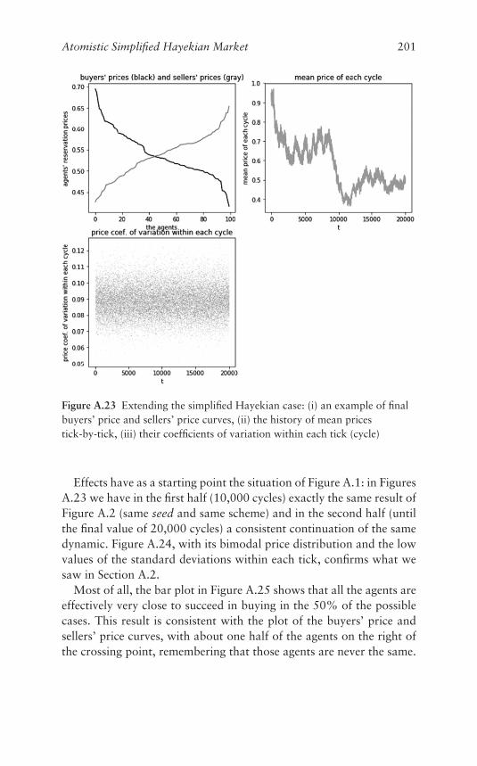
Atomistic Simplified Hayekian Market 201
Figure A.23 Extending the simplified Hayekian case: (i) an example of finalbuyers’ price and sellers’ price curves, (ii) the history of mean pricestick-by-tick, (iii) their coefficients of variation within each tick (cycle)
Effects have as a starting point the situation of Figure A.1: in FiguresA.23 we have in the first half (10,000 cycles) exactly the same result ofFigure A.2 (same seed and same scheme) and in the second half (untilthe final value of 20,000 cycles) a consistent continuation of the samedynamic. Figure A.24, with its bimodal price distribution and the lowvalues of the standard deviations within each tick, confirms what wesaw in Section A.2.
Most of all, the bar plot in Figure A.25 shows that all the agents areeffectively very close to succeed in buying in the 50% of the possiblecases. This result is consistent with the plot of the buyers’ price andsellers’ price curves, with about one half of the agents on the right ofthe crossing point, remembering that those agents are never the same.
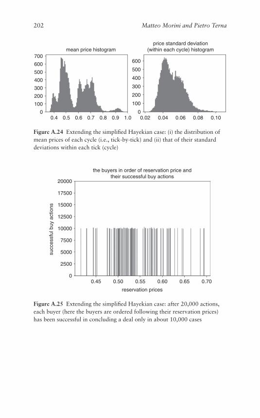
202 Matteo Morini and Pietro Terna
mean price histogramprice standard deviation
(within each cycle) histogram
500
600
700
400
300
200
100
00.5 0.6 0.7 0.8 0.90.4 1.0
500
600
400
300
200
100
00.04 0.06 0.080.02 0.10
Figure A.24 Extending the simplified Hayekian case: (i) the distribution ofmean prices of each cycle (i.e., tick-by-tick) and (ii) that of their standarddeviations within each tick (cycle)
the buyers in order of reservation price andtheir successful buy actions
20000
17500
succ
essf
ul b
uy a
ctio
ns 15000
12500
10000
7500
5000
2500
00.45
reservation prices
0.50 0.55 0.60 0.65 0.70
Figure A.25 Extending the simplified Hayekian case: after 20,000 actions,each buyer (here the buyers are ordered following their reservation prices)has been successful in concluding a deal only in about 10,000 cases
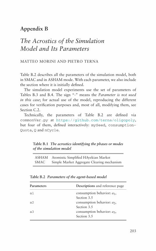
Appendix B
The Acrostics of the SimulationModel and Its Parameters
MATTEO MORINI AND PIETRO TERNA
Table B.2 describes all the parameters of the simulation model, bothin SMAC and in ASHAM mode. With each parameter, we also includethe section where it is initially defined.
The simulation model experiments use the set of parameters ofTables B.3 and B.4. The sign “-” means the Parameter is not usedin this case; for actual use of the model, reproducing the differentcases for verification purposes and, most of all, modifying them, seeSection C.2.
Technically, the parameters of Table B.2 are defined viacommonVar.py at https://github.com/terna/oligopoly,but four of them, defined interactively: mySeed, consumption-Quota, Q and nCycle.
Table B.1 The acrostics identifying the phases or modesof the simulation model
ASHAM Atomistic Simplified HAyekian MarketSMAC Simple Market Aggregate Clearing mechanism
Table B.2 Parameters of the agent-based model
Parameters Descriptions and reference page
a1 consumption behavior: a1,Section 3.5
a2 consumption behavior: a2,Section 3.5
a3 consumption behavior: a3,Section 3.5
203
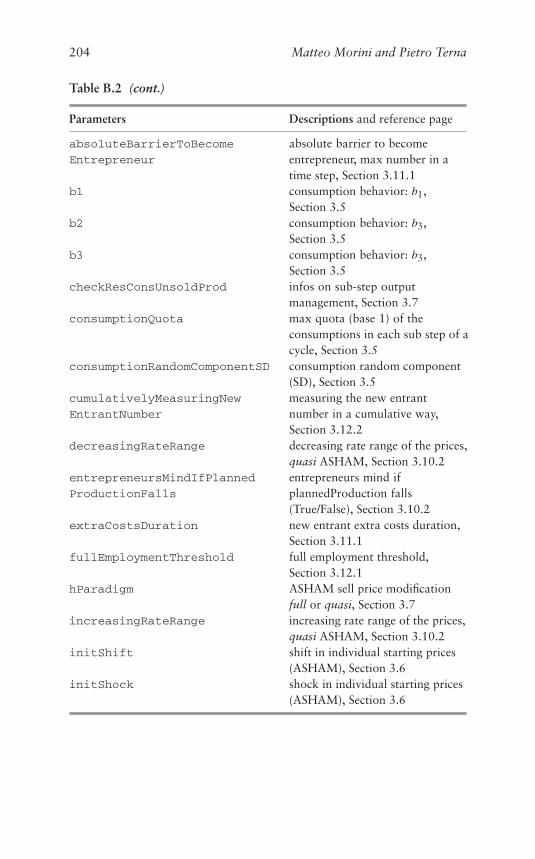
204 Matteo Morini and Pietro Terna
Table B.2 (cont.)
Parameters Descriptions and reference page
absoluteBarrierToBecome
Entrepreneur
absolute barrier to becomeentrepreneur, max number in atime step, Section 3.11.1
b1 consumption behavior: b1,Section 3.5
b2 consumption behavior: b3,Section 3.5
b3 consumption behavior: b3,Section 3.5
checkResConsUnsoldProd infos on sub-step outputmanagement, Section 3.7
consumptionQuota max quota (base 1) of theconsumptions in each sub step of acycle, Section 3.5
consumptionRandomComponentSD consumption random component(SD), Section 3.5
cumulativelyMeasuringNew
EntrantNumber
measuring the new entrantnumber in a cumulative way,Section 3.12.2
decreasingRateRange decreasing rate range of the prices,quasi ASHAM, Section 3.10.2
entrepreneursMindIfPlanned
ProductionFalls
entrepreneurs mind ifplannedProduction falls(True/False), Section 3.10.2
extraCostsDuration new entrant extra costs duration,Section 3.11.1
fullEmploymentThreshold full employment threshold,Section 3.12.1
hParadigm ASHAM sell price modificationfull or quasi, Section 3.7
increasingRateRange increasing rate range of the prices,quasi ASHAM, Section 3.10.2
initShift shift in individual starting prices(ASHAM), Section 3.6
initShock shock in individual starting prices(ASHAM), Section 3.6
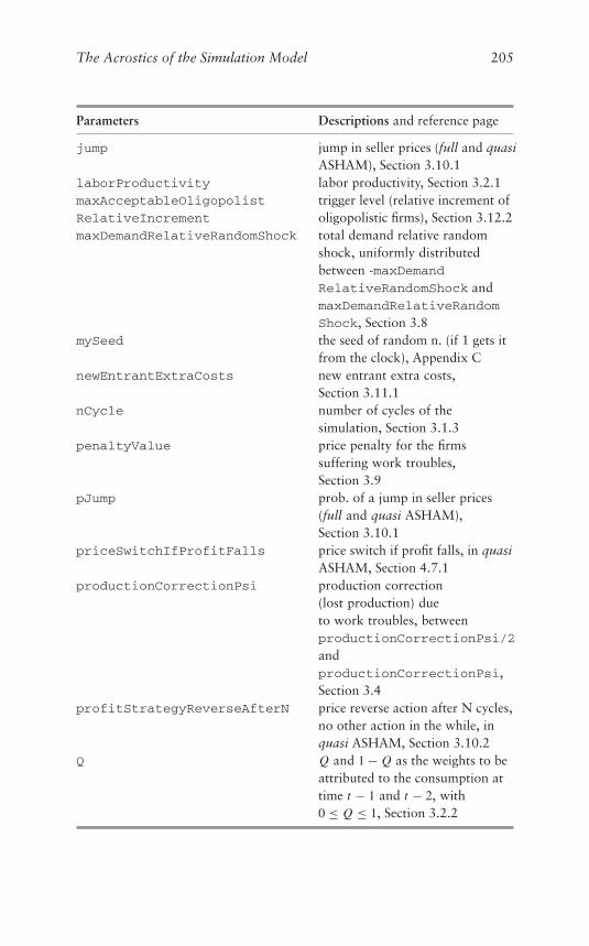
The Acrostics of the Simulation Model 205
Parameters Descriptions and reference page
jump jump in seller prices (full and quasiASHAM), Section 3.10.1
laborProductivity labor productivity, Section 3.2.1maxAcceptableOligopolist
RelativeIncrement
trigger level (relative increment ofoligopolistic firms), Section 3.12.2
maxDemandRelativeRandomShock total demand relative randomshock, uniformly distributedbetween -maxDemandRelativeRandomShock andmaxDemandRelativeRandom
Shock, Section 3.8mySeed the seed of random n. (if 1 gets it
from the clock), Appendix CnewEntrantExtraCosts new entrant extra costs,
Section 3.11.1nCycle number of cycles of the
simulation, Section 3.1.3penaltyValue price penalty for the firms
suffering work troubles,Section 3.9
pJump prob. of a jump in seller prices(full and quasi ASHAM),Section 3.10.1
priceSwitchIfProfitFalls price switch if profit falls, in quasiASHAM, Section 4.7.1
productionCorrectionPsi production correction(lost production) dueto work troubles, betweenproductionCorrectionPsi/2
andproductionCorrectionPsi,Section 3.4
profitStrategyReverseAfterN price reverse action after N cycles,no other action in the while, inquasi ASHAM, Section 3.10.2
Q Q and 1 − Q as the weights to beattributed to the consumption attime t − 1 and t − 2, with0 ≤ Q ≤ 1, Section 3.2.2

206 Matteo Morini and Pietro Terna
Table B.2 (cont.)
Parameters Descriptions and reference page
quasiHchoice quasi ASHAM choice to drivesellers’ price modification,Section 3.10.2
randomComponentOfPlanned
Production
random rel. component ofplanned production uniformlydistributed between -random
ComponentOfPlanned
Production andrandomComponentOfPlanned
Production, Section 3.2.2reUseUnspentConsumption
Capability
reuse unspent consumptioncapability, with a quota in theinterval [0, 1], Section 3.5
rho expected employment ratio att = 1, Section 3.2.1
runningShiftB shift in individual buyer runningprices in ASHAM, Section 3.7
runningShiftS shift in individual seller runningprices in ASHAM, Section 3.7
runningShockB range of the correction of agent (asbuyers) running prices in ASHAM,Section 3.7
runningShockS range of the correction of agent (assellers) running prices in ASHAM,Section 3.7
socialWelfareCompensation social welfare compensation,Section 3.5
soldThreshold1 quasi ASHAM sold threshold tolower the prices, Section 3.10.2
soldThreshold2 quasi ASHAM sold threshold toraise the prices, Section 3.10.2
startHayekianMarket cycle to start the ASHAM phase,Section 3.2.2
temporaryRelativeWage
IncrementAsBarrier
wage relative increment as anentry barrier, Section 3.12.2
thresholdToDecreaseThePriceIf
TotalPlannedPFalls
threshold to decrease the price iftotal planned production falls,case (i), Section 3.10.2
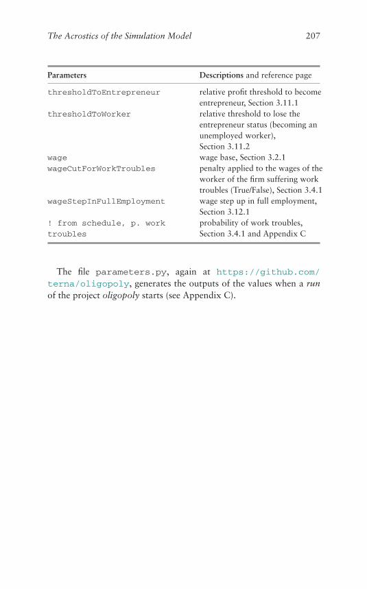
The Acrostics of the Simulation Model 207
Parameters Descriptions and reference page
thresholdToEntrepreneur relative profit threshold to becomeentrepreneur, Section 3.11.1
thresholdToWorker relative threshold to lose theentrepreneur status (becoming anunemployed worker),Section 3.11.2
wage wage base, Section 3.2.1wageCutForWorkTroubles penalty applied to the wages of the
worker of the firm suffering worktroubles (True/False), Section 3.4.1
wageStepInFullEmployment wage step up in full employment,Section 3.12.1
! from schedule, p. work
troubles
probability of work troubles,Section 3.4.1 and Appendix C
The file parameters.py, again at https://github.com/terna/oligopoly, generates the outputs of the values when a runof the project oligopoly starts (see Appendix C).
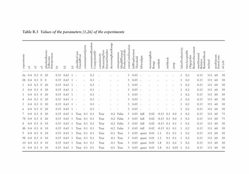
Table B.3 Values of the parameters [1,26] of the experiments
expe
rim
ents
a1 a2 a3 abso
lute
Bar
rier
ToB
ecom
eE
ntre
pren
eur
b1 b2 b3 chec
kRes
Con
sU
nsol
dPro
d
cons
umpt
ionQ
uota
cons
umpt
ionR
ando
mC
ompo
nent
SD
cum
ulat
ivel
yM
easu
ring
New
Ent
rant
Num
ber
decr
easi
ngR
ateR
ange
entr
epre
neur
sM
indI
fPla
nned
Prod
ucti
onFa
lls
extr
aCos
tsD
urat
ion
fullE
mpl
oym
ent
Thr
esho
ld
hPar
adig
m
incr
easi
ngR
ate
Ran
ge
init
Shif
t
init
Shoc
k
jum
p
labo
rPro
duct
ivit
y
max
Acc
epta
ble
Olig
opol
ist
Rel
ativ
eInc
rem
ent
max
Dem
and
Rel
ativ
eR
ando
mSh
ock
myS
eed
new
Ent
rant
Ext
raC
osts
nCyc
le
0a 0.4 0.3 0 20 0.55 0.65 1 - - 0.3 - - - 3 0.05 - - - - - 1 0.2 0.15 111 60 50
0b 0.4 0.3 0 0 0.55 0.65 1 - - 0.3 - - - 3 0.05 - - - - - 1 0.2 0.15 111 60 50
1 0.4 0.3 0 20 0.55 0.65 1 - - 0.3 - - - 3 0.05 - - - - - 1 0.2 0.15 111 60 50
2 0.4 0.3 0 20 0.55 0.65 1 - - 0.3 - - - 3 0.05 - - - - - 1 0.2 0.15 111 60 50
3 0.4 0.3 0 20 0.55 0.65 1 - - 0.3 - - - 3 0.05 - - - - - 1 0.2 0.15 111 60 50
4 0.4 0.3 0 20 0.55 0.65 1 - - 0.3 - - - 3 0.05 - - - - - 1 0.2 0.15 111 60 50
5 0.4 0.3 0 20 0.55 0.65 1 - - 0.3 - - - 3 0.05 - - - - - 1 0.2 0.15 111 60 50
6 0.4 0.3 0 20 0.55 0.65 1 - - 0.3 - - - 3 0.05 - - - - - 1 0.2 0.15 111 60 50
7 0.4 0.3 0 20 0.55 0.65 1 True 0.1 0.1 True -0.2 False 5 0.05 full 0.02 -0.15 0.1 0.0 1 0.2 0.15 111 60 75
7b 0.4 0.3 0 20 0.55 0.65 1 True 0.1 0.1 True -0.2 False 5 0.05 full 0.02 -0.15 0.1 0.0 1 0.2 0.15 111 60 75
8 0.4 0.3 0 10 0.55 0.65 1 True 0.1 0.1 True -0.2 False 5 0.05 full 0.02 -0.15 0.1 0.1 1 0.2 0.15 111 60 50
8b 0.4 0.3 0 10 0.55 0.65 1 True 0.1 0.1 True -0.2 False 5 0.05 full 0.02 -0.15 0.1 0.1 1 0.2 0.15 111 60 50
9 0.4 0.3 0 10 0.55 0.65 1 True 0.1 0.1 True -0.1 True 5 0.05 quasi 0.01 1.1 0.1 0.1 1 0.2 0.15 111 60 50
9b 0.4 0.3 0 10 0.55 0.65 1 True 0.1 0.1 True -0.1 True 5 0.05 quasi 0.01 1.1 0.1 0.1 1 0.2 0.15 111 60 50
10 0.4 0.3 0 10 0.55 0.65 1 True 0.1 0.1 True -0.1 True 5 0.05 quasi 0.01 1.8 0.1 0.2 1 0.2 0.15 111 60 50
11 0.4 0.3 0 10 0.55 0.65 1 True 0.1 0.1 True -0.1 True 5 0.05 quasi 0.01 1.8 0.1 0.05 1 0.2 0.15 111 60 50
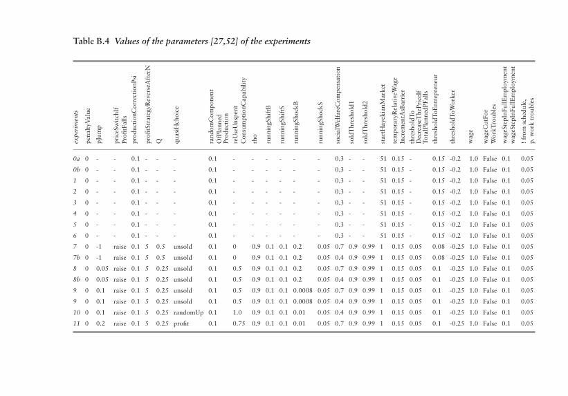
Table B.4 Values of the parameters [27,52] of the experiments
expe
rim
ents
pena
ltyV
alue
pJum
p
pric
eSw
itch
IfPr
ofitF
alls
prod
ucti
onC
orre
ctio
nPsi
profi
tStr
ateg
yRev
erse
Aft
erN
Q quas
iHch
oice
rand
omC
ompo
nent
OfP
lann
edPr
oduc
tion
reU
seU
nspe
ntC
onsu
mpt
ionC
apab
ility
rho
runn
ingS
hift
B
runn
ingS
hift
S
runn
ingS
hock
B
runn
ingS
hock
S
soci
alW
elfa
reC
ompe
nsat
ion
sold
Thr
esho
ld1
sold
Thr
esho
ld2
star
tHay
ekia
nMar
ket
tem
pora
ryR
elat
iveW
age
Incr
emen
tAsB
arri
er
thre
shol
dTo
Dec
reas
eThe
Pric
eIf
Tota
lPla
nned
PFal
ls
thre
shol
dToE
ntre
pren
eur
thre
shol
dToW
orke
r
wag
e
wag
eCut
For
Wor
kTro
uble
s
wag
eSte
pInF
ullE
mpl
oym
ent
wag
eSte
pInF
ullE
mpl
oym
ent
!fr
omsc
hedu
le,
p.w
ork
trou
bles
0a 0 - - 0.1 - - - 0.1 - - - - - - 0.3 - - 51 0.15 - 0.15 -0.2 1.0 False 0.1 0.05
0b 0 - - 0.1 - - - 0.1 - - - - - - 0.3 - - 51 0.15 - 0.15 -0.2 1.0 False 0.1 0.05
1 0 - - 0.1 - - - 0.1 - - - - - - 0.3 - - 51 0.15 - 0.15 -0.2 1.0 False 0.1 0.05
2 0 - - 0.1 - - - 0.1 - - - - - - 0.3 - - 51 0.15 - 0.15 -0.2 1.0 False 0.1 0.05
3 0 - - 0.1 - - - 0.1 - - - - - - 0.3 - - 51 0.15 - 0.15 -0.2 1.0 False 0.1 0.05
4 0 - - 0.1 - - - 0.1 - - - - - - 0.3 - - 51 0.15 - 0.15 -0.2 1.0 False 0.1 0.05
5 0 - - 0.1 - - - 0.1 - - - - - - 0.3 - - 51 0.15 - 0.15 -0.2 1.0 False 0.1 0.05
6 0 - - 0.1 - - - 0.1 - - - - - - 0.3 - - 51 0.15 - 0.15 -0.2 1.0 False 0.1 0.05
7 0 -1 raise 0.1 5 0.5 unsold 0.1 0 0.9 0.1 0.1 0.2 0.05 0.7 0.9 0.99 1 0.15 0.05 0.08 -0.25 1.0 False 0.1 0.05
7b 0 -1 raise 0.1 5 0.5 unsold 0.1 0 0.9 0.1 0.1 0.2 0.05 0.4 0.9 0.99 1 0.15 0.05 0.08 -0.25 1.0 False 0.1 0.05
8 0 0.05 raise 0.1 5 0.25 unsold 0.1 0.5 0.9 0.1 0.1 0.2 0.05 0.7 0.9 0.99 1 0.15 0.05 0.1 -0.25 1.0 False 0.1 0.05
8b 0 0.05 raise 0.1 5 0.25 unsold 0.1 0.5 0.9 0.1 0.1 0.2 0.05 0.4 0.9 0.99 1 0.15 0.05 0.1 -0.25 1.0 False 0.1 0.05
9 0 0.1 raise 0.1 5 0.25 unsold 0.1 0.5 0.9 0.1 0.1 0.0008 0.05 0.7 0.9 0.99 1 0.15 0.05 0.1 -0.25 1.0 False 0.1 0.05
9 0 0.1 raise 0.1 5 0.25 unsold 0.1 0.5 0.9 0.1 0.1 0.0008 0.05 0.4 0.9 0.99 1 0.15 0.05 0.1 -0.25 1.0 False 0.1 0.05
10 0 0.1 raise 0.1 5 0.25 randomUp 0.1 1.0 0.9 0.1 0.1 0.01 0.05 0.4 0.9 0.99 1 0.15 0.05 0.1 -0.25 1.0 False 0.1 0.05
11 0 0.2 raise 0.1 5 0.25 profit 0.1 0.75 0.9 0.1 0.1 0.01 0.05 0.7 0.9 0.99 1 0.15 0.05 0.1 -0.25 1.0 False 0.1 0.05

Appendix C
How to Run the Oligopoly Modelwith SLAPP
MATTEO MORINI AND PIETRO TERNA
The agent-based simulation of Part 2 of this book uses SLAPP (Swarm-Like Agent-based Protocol in Python)1 as shell.2
SLAPP has an open Reference Handbook in its website, and it isthoroughly described in chapters 2–7 of the Boero et al. (2015) book.Chapter 1 of the Reference Handbook describes how to install andhow to run SLAPP (in a trial phase, also without installing it).
Run the Oligopoly project3 with the Python 3 version of SLAPP.Exception: for the two cases of Section 4.1, see the notes in thatsection.
We introduce the starting phase in a detailed way. Please read thefollowing notes in front of your computer.
● We can launch the SLAPP shell in several ways.– As better described in the Reference Handbook4 quoted above,
we can start SLAPP from a terminal, with:python3 runShell.pyvia the runShell.py file, that we can find in the main folder ofSLAPP;
– We can use IPython, mainly in a Jupyter notebook: we goto the main folder of SLAPP and we start jupyter notebookfrom there; then we can launch SLAPP via the iRunShell.ipynb file, simply clicking on it and then starting the executionwith shift+Enter in the first cell of the notebook.
1 https://terna.github.io/SLAPP/ .2 Swarm is the root of many agent-based simulation tools: the article of (Minar
et al., 1996) represents a manifesto of Swarm; we have also two books relatedto Swarm (Luna and Perrone, 2002; Luna and Stefansson, 2012) and we canfind some information online at http://www.swarm.org .
3 http://terna.github.io/oligopoly/ .4 Please see chapter 1 of the Handbook about installing and running SLAPP.
210

How to Run the Oligopoly Model with SLAPP 211
● In both the cases, we are immediately requested to choose a project:Project name?
● We can predefine a default project placing a file namedproject.txt in the folder 6 objectSwarmObserverAgents_AESOP_turtleLib_NetworkX or in the main SLAPP folder;the content of the file is the path to the folder of theproject we are working on (oligopoly in our case, with/Users/pt/GitHub/oligopoly as an example). The initialmessage of SLAPP becomes:
path and project = /Users/pt/GitHub/oligopolydo you confirm? ([y]/n):
● Resuming the explanation, we receive a few technical messages andthen the request:
random number seed (1 to get it from the clock)
– We have to enter an integer number (positive or negative) to ini-tialize the sequence of the random numbers used internally by thesimulation code.
– If we reply 1, the seed used to start the generation of the randomseries comes from the value of the internal clock. So, it is differentanytime we start a simulation run.This reply is useful to replicate the simulated experiments withdifferent outcomes.
– If we chose a number different from 1, the random sequencewould be repeated anytime we will use that seed.This second solution is useful while debugging, when we needto repeat exactly the sequence generating errors, but alsoto give to the user the possibility of replicating exactly anexperiment.
– The seeds used to run the experiments of the book are reportedvia the variable mySeed in Appendix B.
● Parameters: we set the parameters of the model both interactivelyor within the file commonVar.py.
The program reports several messages about the projectparameters, following the content of the file parameters.py;both this file and commonVar.py are in the folder of theproject.
The first message reports the version of the project.
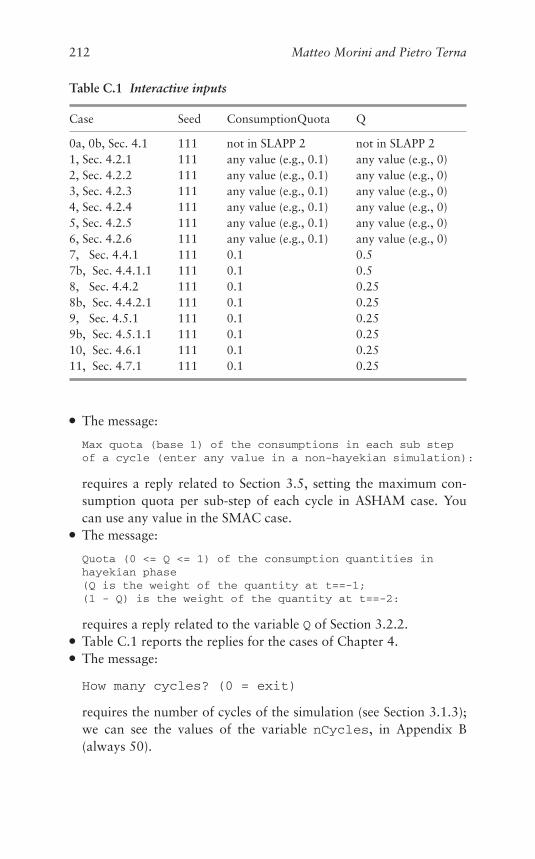
212 Matteo Morini and Pietro Terna
Table C.1 Interactive inputs
Case Seed ConsumptionQuota Q
0a, 0b, Sec. 4.1 111 not in SLAPP 2 not in SLAPP 21, Sec. 4.2.1 111 any value (e.g., 0.1) any value (e.g., 0)2, Sec. 4.2.2 111 any value (e.g., 0.1) any value (e.g., 0)3, Sec. 4.2.3 111 any value (e.g., 0.1) any value (e.g., 0)4, Sec. 4.2.4 111 any value (e.g., 0.1) any value (e.g., 0)5, Sec. 4.2.5 111 any value (e.g., 0.1) any value (e.g., 0)6, Sec. 4.2.6 111 any value (e.g., 0.1) any value (e.g., 0)7, Sec. 4.4.1 111 0.1 0.57b, Sec. 4.4.1.1 111 0.1 0.58, Sec. 4.4.2 111 0.1 0.258b, Sec. 4.4.2.1 111 0.1 0.259, Sec. 4.5.1 111 0.1 0.259b, Sec. 4.5.1.1 111 0.1 0.2510, Sec. 4.6.1 111 0.1 0.2511, Sec. 4.7.1 111 0.1 0.25
● The message:
Max quota (base 1) of the consumptions in each sub stepof a cycle (enter any value in a non-hayekian simulation):
requires a reply related to Section 3.5, setting the maximum con-sumption quota per sub-step of each cycle in ASHAM case. Youcan use any value in the SMAC case.
● The message:
Quota (0 <= Q <= 1) of the consumption quantities inhayekian phase(Q is the weight of the quantity at t==-1;(1 - Q) is the weight of the quantity at t==-2:
requires a reply related to the variable Q of Section 3.2.2.● Table C.1 reports the replies for the cases of Chapter 4.● The message:
How many cycles? (0 = exit)
requires the number of cycles of the simulation (see Section 3.1.3);we can see the values of the variable nCycles, in Appendix B(always 50).
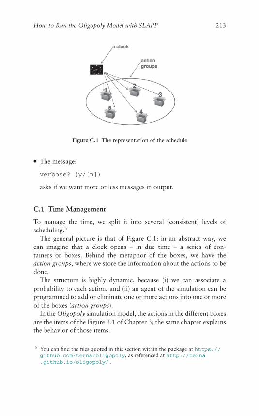
How to Run the Oligopoly Model with SLAPP 213
Figure C.1 The representation of the schedule
● The message:
verbose? (y/[n])
asks if we want more or less messages in output.
C.1 Time Management
To manage the time, we split it into several (consistent) levels ofscheduling.5
The general picture is that of Figure C.1: in an abstract way, wecan imagine that a clock opens – in due time – a series of con-tainers or boxes. Behind the metaphor of the boxes, we have theaction groups, where we store the information about the actions to bedone.
The structure is highly dynamic, because (i) we can associate aprobability to each action, and (ii) an agent of the simulation can beprogrammed to add or eliminate one or more actions into one or moreof the boxes (action groups).
In the Oligopoly simulation model, the actions in the different boxesare the items of the Figure 3.1 of Chapter 3; the same chapter explainsthe behavior of those items.
5 You can find the files quoted in this section within the package at https://github.com/terna/oligopoly, as referenced at http://terna.github.io/oligopoly/ .

214 Matteo Morini and Pietro Terna
C.1.1 The Schedule.xls Formalism
The choice of SLAPP is that of using the spreadsheet formalism todefine the sequence of the events in a detailed way.
The file schedule.xls, which is in the folder of each project,reports this kind of information. SLAPP translates its content in plaintext, reported into the file schedule.txt; if we eliminate the fileschedule.xls, we can use directly the schedule.txt one, but itis a more difficult task than working via the spreadsheet.
● This kind of script does not exist in Swarm, so it is a specific fea-ture of SLAPP, introduced as implementation of the AESOP (Agentsand Emergencies for Simulating Organizations in Python) idea: alayer that describes in a fine-grained way the actions of the agentsin a simulation model. More details are in the SLAPP ReferenceHandbook at https://terna.github.io/SLAPP/ .
● The file schedule.xls can be composed of several sheets, with:(a) the first one with schedule as mandatory name; (b) the othersheets with any name (those names are macro instruction names).We can recall the macro instructions in any sheet, but not within thesheet that creates the macro (that with the same name of the macro),to avoid infinite loops.
● Within the sheets, we have the action groups, as introduced above(Figure C.1), starting with the sign #, followed by a group identifierwhich is also its position in the time sequence.
In schedule.xls we have:
● the first column reporting the acting agent/agents;● the second column reporting the action/instruction;
– if in the second column we find a (positive) number,6 it representsthe probability of activation of the action/instruction reported inthe third column;
– if in the second column we read computationalUse, theorder of the third column is a special computational use ofthe WordState of the first column. WordState has to beinterpreted as an abstract agent;
6 In the above quoted Handbook of SLAPP, we also introduce negative numbersin this position, but we never use that feature within the Oligopoly model.

How to Run the Oligopoly Model with SLAPP 215
● optional comments are placed in the fifth column (here notreported).
Our schedule is:
# 1 100entrepreneurs makeProductionPlanentrepreneurs adaptProductionPlanV6entrepreneurs hireFireWithProductionentrepreneurs 0.05 workTroublesentrepreneurs produceV5entrepreneurs planConsumptionInValueV6workers planConsumptionInValueV6all setInitialPricesHMmacro actWorldState computationalUse setMarketPriceV6entrepreneurs evaluateProfitV6entrepreneurs nextSellPriceJumpFHMentrepreneurs nextSellPricesQHMworkers toEntrepreneurV6entrepreneurs toWorkerV3WorldState computationalUse fullEmployment
EffectOnWagesWorldState computationalUse incumbentAction
OnWages
In schedule.xls we have a second sheet named act, reportingthe content of the macro:
all actOnMarketPlaceall actOnMarketPlaceall actOnMarketPlaceall actOnMarketPlaceall actOnMarketPlace...
The number of repetition of the method actOnMarketPlace ineach cycle is determined by the number of rows in the macro sheetact.# 1 100 means from t = 1 to t = 100, but the experiments
reported in the book are limited to 50 or 75 steps.If the row starts with:
● entrepreneurs, the instruction of the script is operating with theentrepreneurs;
● workers, the instruction of the script is operating with theworkers;
216 Matteo Morini and Pietro Terna
● all, the instruction of the script is operating both with theentrepreneurs and the workers;
● macro, the script jumps to the sheet with the specific name, toexecute the actions reported there;
● WorldState, the instruction of the script is operating with theabstract agent WorldState, as in Sections 3.8, 3.12.1, and 3.12.2.
The instructions are:
● makeProductionPlan, defined in Section 3.2.1 and reported asitem 1 in Figure 3.1;
● adaptProductionPlanV6, defined in Section 3.2.2 and reportedas item 2 in Figure 3.1;
● hireFireWithProduction, defined in Section 3.3 and reportedas item 3 in Figure 3.1;
● workTroubles, defined in Section 3.4.1 and reported within item4 in Figure 3.1;
● produceV5, defined in Section 3.4 and reported as item 4 inFigure 3.1;
● planConsumptionInValueV6, defined in Section 3.5 andreported as item 5 in Figure 3.1;
● setInitialPricesHM, defined in Section 3.6 and reported asitem 6 in Figure 3.1;
● act, the macro activating actOnMarketPlace;● actOnMarketPlace, defined in Section 3.7 and reported as item
7 in Figure 3.1;● setMarketPriceV6, defined in Section 3.8 and reported as item
8 in Figure 3.1;● evaluateProfitV6, defined in Section 3.9 at and reported as
item 9 in Figure 3.1;● nextSellPriceJumpFHM, defined in Section 3.10.1 at and
reported as item 10 full in Figure 3.1;● nextSellPricesQHM, defined in Section 3.10.2 and reported as
item 10 quasi in Figure 3.1;,● toEntrepreneurV6, defined in Section 3.11.1 and reported as
item 11 in Figure 3.1;● toWorkerV3, defined in Section 3.11.2 and reported as item 11 in
Figure 3.1;● fullEmploymentEffectOnWages, defined in Section 3.12.1 and
reported as item 12 in Figure 3.1;

How to Run the Oligopoly Model with SLAPP 217
● incumbentActionOnWages, defined in Section 3.12.2 andreported as item 12 in Figure 3.1;
C.1.2 The observerActions and modelActions as High LevelSchedule Formalisms
Formalism of observerActions.
● The file observerActions.txt reports the first high-level sched-ule formalism; the content (row changes are not relevant in this kindof files) is:– version without pauses contained in observerActions nopause.txt, to be copied to observerActions.txt to runit:collectStructuralData modelStep collectTimeSeriesvisualizePlot visualizeNet clock
– version with pauses contained in observerActions withpause.txt, to be copied to observerActions.txt to runit:collectStructuralData modelStep collectTimeSeriesvisualizePlot visualizeNet pause clock
The interpretation is the following.– The execution of the contents of the file is “with repetition,” until
an end item will appear (see below).– collectStructuralData collects the number of workers and
of entrepreneurs at the beginning of each period, both as a basisfor internal calculations and for the final output of the model,when two files of data are generated.
– modelStep orders to the model to make a step forward in time.– collectTimeSeries collects the data of the outcomes of the
simulation at the end of each period, both as a basis for the actionvisualizePlot and for the final output of the model, whentwo files of data are generated.
– visualizePlot update the plot of the time series generated bythe model.
– visualizeNet updates the plot of the links connectingentrepreneurs and workers, on a network basis.
– pause, if any, puts the program in wait until we reply to themessage Hit enter key to continue, e.g., hitting the key
218 Matteo Morini and Pietro Terna
. This action is useful to examine the graphical outputs stepby step.
– clock asks to the clock to increase its counter of one unit.When the count will reach the value we have entered replyingto the How many cycles? query, the internal scheduler of theObserver will add the end item into the sequence of the fileobserverActions.txt. The item is placed immediately afterthe clock call. The end item stops the sequence contained in thefile.
– We can also consider a potential prune item, eliminating thelinks connecting entrepreneurs and workers on the basis of theirweight (optionally asking for a threshold below which to makethe elimination); weights could be introduced to measure theseniority, the skills, or the experience of the workers.
Formalism of modelActions.
● The file modelActions.txt reports the second high-level sched-ule formalism; the content (row changes are not relevant in this kindof files) is:
reset read_script
The interpretation is the following:– Also at the Model level the execution of the content of the file is
“with repetition,” never ending. It is the Observer that stops thesimulation run, but operating at its level.
– reset orders to the agents to make a reset of their variables, ifnecessary.
– read_script orders to the Model to execute the sequence ofinstructions of the file schedule.xls.
C.2 Running a Specific Experiment, with BackwardCompatibility
● To run the experiments of the cases 0a and 0b, we need to use theOligopoly code version V5 or V5bP2_fd,7 running the project with
7 At https://github.com/terna/oligopoly/releases/tag/V5 or athttps://github.com/terna/oligopoly/releases/tag/V5bP2_fd .

How to Run the Oligopoly Model with SLAPP 219
SLAPP 2.0, which is at https://github.com/terna/SLAPP2and controlling that the parameters are those of rows 1 and 2 ofTables B.3 and B.4. In this case, using that SMAC specific versionof the Oligopoly project, the startHayekianMarket parameter is notused, while in the Table B.4 is set to 51 by default.
To set the correct parameters, for the cases 0a and 0b, you cansimply modify the parameter absoluteBarrierToBecomeEntrepreneur at row 123 of the file commonVar.py of the abovereleases of Oligopoly, setting it to 20 (case 0a) or to 0 (case 0b).
The path to the folder containing the Oligopoly code has to beincluded in a file named project.txt, to be placed into the mainfolder of SLAPP.
● For all the cases below, please use the Oligopoly code of the releaseV6book, or directly the branch master, running the project withSLAPP 3.0 or higher, which is at https://github.com/terna/SLAPP3 .
As above, the path to the folder containing the Oligopoly codehas to be included in a file named project.txt, to be placed into themain folder of SLAPP.
● To run the experiments of the cases from 1 to 6:
a) delete the file schedule.xls;b) duplicate the file schedule5.xls;c) rename the result as schedule.xls;d) for each specific experiment:
– delete the files commonVar.py, workers.txtx, entrepreneurs.txt (if any), entrepreneurs.txtx (if any);
– for case X , duplicate the files commonVar.py.caseX,workers.txtx.caseX, entrepreneurs.txt.caseX orentrepreneurs.txtx.caseX;
– rename the results as commonVar.py, workers.txtx,entrepreneurs.txt or entrepreneurs.txtx.
● To run the experiments of the cases 7 and 7b:
a) delete the file schedule.xls;b) duplicate the file schedule6.xls.backwardCompatibily;c) rename the result as schedule.xls;d) for each specific experiment:
– delete the files commonVar.py, workers.txtx, entrepreneurs.txt (if any), entrepreneurs.txtx (if any);
220 Matteo Morini and Pietro Terna
– for case X , duplicate the files commonVar.py.caseX,workers.txtx.caseX, entrepreneurs.txt.caseX orentrepreneurs.txtx.caseX;
– rename the results as commonVar.py, workers.txtx,entrepreneurs.txt or entrepreneurs.txtx.
● The experiments from 1 to 7 also run without the modificationsabove, but producing slightly different results.
● To run the experiments of the cases from 8 upward:a) if you made one of the modifications above:
– delete the file schedule.xls;– duplicate the file schedule6.xls;– rename the result as schedule.xls;
b) for each specific experiment:– delete the files commonVar.py, workers.txtx, entrepreneurs.txt (if any), entrepreneurs.txtx (if any);
– for case *X*, duplicate the files commonVar.py.caseX,workers.txtx.caseX, entrepreneurs.txt.caseX orentrepreneurs.txtx.caseX;
– rename the results as commonVar.py, workers.txtx,entrepreneurs. txt or entrepreneurs.txtx.
● The experiments from 1 to 7 also run without the modificationsreported above, but producing slightly different results.
● Each case requires the input of a few parameters in an interactiveway. We report them in Table C.1.
C.3 Running the Code Directly Online
It is possible to run the Oligopoly project directly online, viahttps://mybinder.org, accessing the file system at https://mybinder.org/v2/gh/terna/SLAPP3/master to modify – ifnecessary – the content of the folder oligopoly contained into thefolder6 objectSwarmObserverAgents_AESOP_turtleLib_NetworkX.
Then, from the main folder, we launch the iRunShellOnline.ipynb file, and finally we follow the instructions contained in it.
The final part of the file runningSpecificCases.md athttps://github.com/terna/oligopoly contains instructionsto run the code using other online resources.
References
Acemoglu, D., Carvalho, V. M., Ozdaglar, A., and Tahbaz-Salehi, A. 2012.The network origins of aggregate fluctuations. Econometrica, 80(5),1977–2016.
Aguirregabiria, V., and Mira, P. 2007. Sequential estimation of dynamicdiscrete games. Econometrica, 75(1), 1–53.
Allen, B., and Hellwig, M. 1986. Bertrand-Edgeworth oligopoly in largemarkets. The Review of Economic Studies, 53(2), 175–204.
Aoki, M., and Yoshikawa, H. 2007. Reconstructing macroeconomics: a per-spective from statistical physics and combinatorial stochastic processes.Cambridge University Press.
Axtell, R. 2000. Why agents? On the varied motivations for agent com-puting in the social sciences. Center on Social and Economic Dynamics –working paper.
Axtell, R. L., and Epstein, J. M. 2006. Coordination in transient social net-works: an agent-based computational model of the timing of retirement.In: Epstein, J. M. (ed), Generative social science: Studies in agent-basedcomputational modeling, 146–74. Princeton, NJ: Princeton UniversityPress.
Bagliano, F. C., and Bertola, G. 2004. Models for dynamic macroeconomics.Oxford University Press.
Bertoletti, P., and Etro, F. 2016. Preferences, entry, and market structure.The RAND Journal of Economics, 47(4), 792–821.
Bilbiie, F. O., Ghironi, F., and Melitz, M. J. 2012. Endogenous entry, prod-uct variety, and business cycles. Journal of Political Economy, 120(2),304–45.
Blinder, A. 1986. A skeptical note on the new econometrics. In: Preston,M., and Quandt, R. (eds), Prices, competition and equilibrium, 73–83.Oxford: Phillip Allan Publishers.
Boero, R., Morini, M., Sonnessa, M., and Terna, P. 2015. Agent-based mod-els of the economy – from theories to applications. Palgrave Macmillan.
Bowles, S., Kirman, A., and Sethi, R. 2017. Retrospectives: Friedrich Hayekand the market algorithm. Journal of Economic Perspectives, 31(3),215–30.
221
222 References
Branch, W. A., and McGough, B. 2010. Dynamic predictor selection ina new Keynesian model with heterogeneous expectations. Journal ofEconomic Dynamics and Control, 34(8), 1492–508.
Branch, W. A., and McGough, B. 2016. Heterogeneous expectations andmicro-foundations in macroeconomics. In: Hommes, C., and LeBaron, B.(eds), Handbook of computational economics, 3–62. Elsevier Handbooksin Economics Series, Arrow, K., Woodford, M., Rotemberg, J. (eds), vol.4, Heterogeneous Agent Models. Amsterdam: Elsevier.
Carvalho, V., and Gabaix, X. 2013. The great diversification and itsundoing. American Economic Review, 103(5), 1697–727.
Christiano, L. J., Eichenbaum, M. S., and Trabandt, M. 2018. On DSGEmodels. Journal of Economic Perspectives, 32(3), 113–40.
Chu, A. C., and Ji, L. 2016. Monetary policy and endogenous marketstructure in a Schumpeterian economy. Macroeconomic Dynamics, 20(5),1127–45.
Clementi, G. L., and Palazzo, B. 2016. Entry, exit, firm dynamics, andaggregate fluctuations. American Economic Journal: Macroeconomics,8(3), 1–41.
Comin, D., and Gertler, M. 2006. Medium-term business cycles. AmericanEconomic Review, 96(3), 523–51.
Corbellini, A., Crosato, L., Ganugi, P., and Mazzoli, M. 2010. FittingPareto II distributions on firm size: Statistical methodology and economicpuzzles. In Skiadas, C. H. (ed), Advances in data analysis: Theory andapplications to reliability and inference, data mining, bioinformatics,lifetime data and neural networks, 321–8. Springer.
Dasgupta, P., and Maskin, E. 1986. The existence of equilibrium in dis-continuous economic games, Part I (Theory). The Review of EconomicStudies, 53(1), 1–26.
De Grauwe, P. 2011. Animal spirits and monetary policy. EconomicTheory, 47(2–3), 423–57.
De Grauwe, P., and Kaltwasser, P. R. 2012. Animal spirits in the foreignexchange market. Journal of Economic Dynamics and Control, 36(8),1176–92.
Delli Gatti, D., Desiderio, S., Gaffeo, E., Cirillo, P., and Gallegati, M.2011. Macroeconomics from the bottom-up. Vol. 1. Springer Science &Business Media.
Delli Gatti, D., Di Guilmi, C., Gaffeo, E., et al. 2005. A new approach tobusiness fluctuations: heterogeneous interacting agents, scaling laws andfinancial fragility. Journal of Economic Behavior & Organization, 56(4),489–512.
Delli Gatti, D., Gallegati, M., Greenwald, B., Russo, A., and Stiglitz, J. E.2010. The financial accelerator in an evolving credit network. Journal ofEconomic Dynamics and Control, 34(9), 1627–50.
References 223
Di Guilmi, C., Gallegati, M., and Landini, S. 2017. Interactivemacroeconomics: stochastic aggregate dynamics with heterogeneousand interacting agents. Cambridge University Press.
Dilaver, Ö., Calvert Jump, R., and Levine, P. 2018. Agent-basedmacroeconomics and dynamic stochastic general equilibrium mod-els: Where do we go from here? Journal of Economic Surveys, 32(4),1134–59.
Dosi, G., Fagiolo, G., and Roventini, A. 2006. An evolutionary model ofendogenous business cycles. Computational Economics, 27(1), 3–34.
Dosi, G., Fagiolo, G., and Roventini, A. 2008. The microfoundationsof business cycles: an evolutionary, multi-agent model. Journal ofEvolutionary Economics, 18(3–4), 413.
Dosi, G., Fagiolo, G., and Roventini, A. 2010. Schumpeter meeting Keynes:A policy-friendly model of endogenous growth and business cycles.Journal of Economic Dynamics and Control, 34(9), 1748–67.
Dosi, G., and Roventini, A. 2017. Agent-based macroeconomics andclassical political economy: some Italian roots. Italian Economic Journal,3(3), 261–83.
Dunne, T., Klimek, S. D., Roberts, M. J., and Xu, D. Y. 2013. Entry,exit, and the determinants of market structure. The RAND Journal ofEconomics, 44(3), 462–87.
Epstein, J. 2008. Why model? Journal of Artificial Societies and SocialSimulation, 11(4), 12.
Etro, F., and Colciago, A. 2010. Endogenous market structures and thebusiness cycle. The Economic Journal, 120(549), 1201–33.
Fagiolo, G., Moneta, A., and Windrum, P. 2007. A Critical Guide toEmpirical Validation of Agent-Based Models in Economics: Methodolo-gies, Procedures, and Open Problems. Computational Economics, 30(3),195–226.
Fagiolo, G., and Roventini, A. 2017. Macroeconomic Policy in DSGE andAgent-Based Models Redux: New Developments and Challenges Ahead.Journal of Artificial Societies and Social Simulation, 20(1), 1.
Forni, M., and Lippi, M. 1997. Aggregation and the microfoundations ofdynamic macroeconomics. Oxford University Press.
Gabaix, X. 2011. The granular origins of aggregate fluctuations.Econometrica, 79(3), 733–72.
Gaffeo, E., Delli Gatti, D., Desiderio, S., and Gallegati, M. 2008. Adaptivemicrofoundations for emergent macroeconomics. Eastern EconomicJournal, 34(4), 441–63.
Galí, J. 2002. New perspectives on monetary policy, inflation, and thebusiness cycle. National Bureau of Economic Research Working PaperNo. 8767.
224 References
Galí, J. 2008. Monetary policy, inflation, and the business cycle: an intro-duction to the new Keynesian framework. Princeton University Press.
Gertner, R. 1985. Simultaneous move price-quantity games and non-marketclearing equilibrium. Essays in Theoretical Industrial Organization.PhD thesis, Massachusetts Institute of Technology, Department ofEconomics.
Ghorbani, A., Dechesne, F., Dignum, V., and Jonker, C. 2014. EnhancingABM into an inevitable tool for policy analysis. Policy and ComplexSystems, 1(1), 61–76.
Grassi, B., and Carvalho, V. 2015. Firm dynamics and the granularhypothesis. In: 2015 Meeting Papers, Society for Economic Dynamics.
Harsanyi, J. C. 1973. Games with randomly disturbed payoffs: A newrationale for mixed-strategy equilibrium points. International Journal ofGame Theory, 2(1), 1–23.
Hayek, F. A. 1994. Hayek on Hayek: an autobiographical dialogue. Vol.edited by Stephen Kresge and Leif Wenar. University of Chicago Press.
Jaimovich, N., and Rebelo, S. 2009. Can news about the future drive thebusiness cycle? American Economic Review, 99(4), 1097–118.
Kirman, A. P. 1992. Whom or what does the representative individualrepresent? Journal of Economic Perspectives, 6(2), 117–36.
Kreps, D. M., and Scheinkman, J. A. 1983. Quantity precommitmentand Bertrand competition yield Cournot outcomes. The Bell Journal ofEconomics, 326–37.
Kuznets, S. 1946. National product since 1869. National Bureau ofEconomic Research.
Lee, Y., and Mukoyama, T. 2018. A model of entry, exit, and plant-leveldynamics over the business cycle. Journal of Economic Dynamics andControl, 96, 1–25.
Lengnick, M. 2013. Agent-based macroeconomics: A baseline model.Journal of Economic Behavior & Organization, 86, 102–20.
Lorenzoni, G. 2009. A theory of demand shocks. American EconomicReview, 99(5), 2050–84.
Loury, G. C. 1979. Market structure and innovation. The QuarterlyJournal of Economics, 93(3), 395–410.
Lucas, R. J. 1976. Econometric policy evaluation. A critique. In: Brunner,K., and Meltzer, A. (eds), The Phillips curve and labour market, vol.1, Carnegie-Rochester Series on Public Policy, Journal of MonetaryEconomics, Suppl., 10–46. North-Holland.
Luna, F., and Perrone, A. 2002. Agent-based methods in economics andfinance: simulations in Swarm. Vol. 17. Springer Science & BusinessMedia.

References 225
Luna, F., and Stefansson, B. 2012. Economic simulations in Swarm: Agent-based modelling and object oriented programming. Vol. 14. SpringerScience & Business Media.
Madden, P. 1998. Elastic demand, sunk costs and the Kreps–Scheinkmanextension of the Cournot model. Economic Theory, 12(1), 199–212.
Malleson, N. 2018. Validating ABMs (SIMSOC discussion). http://surf.leeds.ac.uk/announce/2018/10/02/Validation_of_ABMs.html, accessed October 13, 2018.
Manjón-Antolín, M. C. 2010. Firm size and short-term dynamics in aggre-gate entry and exit. International Journal of Industrial Organization,28(5), 464–76.
Maskin, E. 1986. The existence of equilibrium with price-setting firms. TheAmerican Economic Review, 76(2), 382–6.
Mazzoli, M., Morini, M., and Terna, P. 2017. Business cycle in amacromodel with oligopoly and agents’ heterogeneity: an agent-basedapproach. Italian Economic Journal, 5, 1–29.
McCallum, B. T., and Nelson, E. 1999. An optimizing IS-LM specificationfor monetary policy and business cycle analysis. Journal of Money,Credit, and Banking, 31(3), 296–316.
Minar, N., Burkhart, R., Langton, C., and Askenazi, M. 1996. The SwarmSimulation System: A toolkit for building multi-agent simulations. SFIWorking Paper, 06(42).
Newell, A., and Simon, H. A. 1972. Human problem solving. Prentice-Hall.Osborne, M., and Rubinstein, A. 1994. A course in game theory. MIT Press.Romer, P. 2016. The trouble with macroeconomics. The American
Economist.Sutton, J. 1998. Technology and market structure: theory and history. MIT
press.Sutton, J. 2002. The variance of firm growth rates: the ‘scaling’ puzzle.
Physica A: Statistical Mechanics and Its Applications, 312(3–4), 577–90.Sutton, J. 2003. The variance of corporate growth rates. Physica A:
Statistical Mechanics and Its Applications, 324(1–2), 45–8.Sutton, J. 2007. Market share dynamics and the “persistence of leadership”
debate. American Economic Review, 97(1), 222–41.Trichet, J.-C. 2010. Reflections on the nature of monetary policy non-
standard measures and finance theory. Opening address at the ECBCentral Banking Conference, Frankfurt, November 18, 2010. http://ww.ecb.europa.eu/press/key/date/2010/html/sp101118.en.html, accessed December 1, 2018.
Veracierto, M. 2008. Firing costs and business cycle fluctuations.International Economic Review, 49(1), 1–39.

226 References
Veracierto, M. L. 2002. Plant-level irreversible investment and equilibriumbusiness cycles. American Economic Review, 92(1), 181–97.
Vives, X. 2001. Oligopoly pricing: old ideas and new tools. MIT Press.Walsh, C. E. 2017. Monetary theory and policy. MIT Press.Weidlich, A., and Veit, D. 2008. Agent-based modeling of oligopolistic
competition in the German electricity market. In: Möst, D., Fichtner,W., Ragwitz, M., and Veit, D. (eds), New methods for energy marketmodelling: proceedings of the First European Workshop on EnergyMarket Modelling Using Agent Based Computational Economics, 3–13.KIT Scientific Publishing.
Wiesner, K., Birdi, A., Eliassi-Rad, T., et al. 2019. Stability of democracies:a complex systems perspective. European Journal of Physics, 40(1),014002.
Author Index
Allen, B., 64Axtell, R., 77
Bertoletti, P., 28Bowles, S., 79
Epstein, J.M., 77Etro, F., 28
Galì, J.C., 19, 29
Hayek, F.A., 79, 181Hellwig, M., 64
Kirman, A., 79Kreps, D., 28
Lucas, R.E. Jr., 16
Madden, P., 28Manjón-Antolín, M.C., 26
Scheinkman, J., 28Sethi, R., 79
Walsh, C.E., 29
227
Subject Index
ν calculation, 85ASHAM, 79SMAC, 79
a source of inspiration, 198abstract agent and computations, 96,
103acrostics, 203action groups, 214actOnMarketPlace, 92adaptProductionPlan
ASHAM, 86adapting the production plan eq.,
87SMAC, 85
adapting the production plan eq.,86
AEA Data Availability Policy, 7, 79agent-based models, 77Aggregate demand, 28ASHAM
full, 138quasi, profit option, 158quasi, random Up option, 153quasi, unsold option, 147
ASHAM experiments, 136
backward compatibility, 218buyers and sellers unbalancing number,
185
case 0aagent series, 108macro-variable series, 108
case 0bagent series, 109macro-variable series, 109
case 1
agent series, 114macro-variable series, 113
case 10agent series, 156macro-variable series, 156
case 11agent series, 161macro-variable series, 161
case 2agent series, 116macro-variable series, 116
case 3agent series, 118macro-variable series, 118
case 4agent series, 121macro-variable series, 120
case 5agent series, 124macro-variable series, 124
case 6agent series, 126macro-variable series, 126
case 7agent series, 141macro-variable series, 140
case 7bmacro-variable series, 143
case 8agent series, 146macro-variable series, 145
case 8bmacro-variable series, 147
case 8modParsagent series, 166macro-variable series, 166
case 9agent series, 151
228

Subject Index 229
macro-variable series, 150case 9b
agent series, 154macro-variable series, 153
clusters in SMAC cases, 134collectStructuralData, 217collectTimeSeries, 217correcting production due to work
problems, 88correcting wage level due to work
problems, 88cycle, 84, 182
demand functionV3 with a negativeshock, 96
demand functionV3 with a positiveshock, 96
dictionary of method probabilities, 88
Employment, 48Entry, 48evaluateProfit, 97Exit, 48
Firms, 39full employment, 103full paradigm, 81fullEmploymentEffectOnWages, 103fullEmploymentEffectOnWages and
incumbentActionOnWages, 103
hireFireWithProduction, 87How to run the Oligopoly project with
SLAPP, 210
Incentive compatible wage, 48incumbentActionOnWages, 103Initial results coming from a previous
work, 106initialBuyPriceCorrection1, 91initialBuyPriceCorrection2, 91initialSellPriceCorrection1, 91initialSellPriceCorrection2, 91item
1, 8410, 98
full, 98quasi, 99
11, 102toEntrepreneur, 102
toWorker, 10212, 103
fullEmploymentEffectOnWages,103
incumbentActionOnWages, 1032
adaptProductionPlan, 843, 874, 87
continuation, 885, 886, 897, 928, 969, 97
jump in full ASHAM, 99jump in quasi HM, 100
legends in time series figures andcorrelation tables, 107
makeProductionPlan, 84max quantity of consumption per sub
step, 89modelStep, 217
nBuyers � nSellers with different ratesof per-capita correction, 192
nBuyers � nSellers with unequal ratesof per-capita correction, butsqueezing the effects, 196
nBuyers � nSellers with unequal ratesof per-capita correction, withequivalent effects, 193
nBuyers GT nSellers with differentrates of per-capita correction,187
nBuyers GT nSellers with unequalrates of per-capita correction,but squeezing the effects, 189
nBuyers GT nSellers with unequalrates of per-capita correction,with equivalent effects, 187
negative consumption, 89nextSellPriceJumpFHM, 98nextSellPricesQHM, 99
observerActions and modelActions,217
230 Subject Index
offer curves, a warning, 81, 136, 137online, 220
parameter set, 203parameters, 211penalty value, 97planConsumptionInValue, 88planned consumptions, 88planned consumptions plus, 89predefining a default project, 211price corrections in the ASHAM phase,
94produce, 87production version 0, 87profit in ASHAM, 98profit in SMAC, 98profitStrategyReverseAfterN cases, 101
quasi paradigm, 81
random values On and Off, 163read_script, 218realistic simulated prices, 183report about residual consumption in
value and unsold production inquantity, 96
required labor force, 87reset, 84, 218reset wages, 103, 104result replication, 7, 79running a specific experiment, 218runningBuyPriceDownCorrection1, 94runningBuyPriceDownCorrection2, 95runningBuyPriceUpCorrection1, 95runningBuyPriceUpCorrection2, 95runningSellPriceDownCorrection1, 95runningSellPriceDownCorrection2, 95runningSellPriceUpCorrection1, 95
runningSellPriceUpCorrection2, 95
Scatter plot of SMAC cases, 132schedule.xls, 214seed of the random numbers, 211setInitialPricesHM, 89setMarketPrice, 96simulation outline, 80SLAPP – Swarm-Like Agent Protocol
in Python, 78SMAC synopsis of different markets,
112space of the parameters, 106structure of a Simplified Hayekian
Market, 139, 181structure of the micro Hayekian
model, 181sub-steps, 84Summarizing countercyclical markup
presence in cases 0a to 6, 127symmetric corrections, 92Synopsis of cases 0a to 6, 127Synopsis of cases 7 to 11, 163
time management, 213toEntrepreneur, 102toEntrepreneur and toWorker, 102toWorker, 102
unexpected by-product: the solution ishere, 200
unique kind of good, 84
visualizeNet, 217visualizePlot, 217
Wage, 48workTroubles, 88