Rethinking Experience Replay:a Bag of Tricks for Continual Learning

Pietro Buzzega∗, Matteo Boschini∗, Angelo Porrello and Simone CalderaraUniversity of Modena and Reggio Emilia, Italy

Email: {pietro.buzzega, matteo.boschini, angelo.porrello, simone.calderara}@unimore.it

Abstract—In Continual Learning, a Neural Network is trainedon a stream of data whose distribution shifts over time. Underthese assumptions, it is especially challenging to improve onclasses appearing later in the stream while remaining accurate onprevious ones. This is due to the infamous problem of catastrophicforgetting, which causes a quick performance degradation whenthe classifier focuses on learning new categories. Recent literatureproposed various approaches to tackle this issue, often resortingto very sophisticated techniques. In this work, we show thatnaive rehearsal can be patched to achieve similar performance.We point out some shortcomings that restrain Experience Replay(ER) and propose five tricks to mitigate them. Experiments showthat ER, thus enhanced, displays an accuracy gain of 51.2 and26.9 percentage points on the CIFAR-10 and CIFAR-100 datasetsrespectively (memory buffer size 1000). As a result, it surpassescurrent state-of-the-art rehearsal-based methods.

I. INTRODUCTION

Deep Neural Networks represent a valid tool for classi-fication tasks, showing excellent performance on a varietyof domains. However, this holds when all training data areimmediately available and identically distributed, a condi-tion that is hard to find outside an artificial environment.In a practical application, new classes may emerge later inthe stream: simply fine-tuning on them would disrupt thepreviously acquired knowledge quickly. This is known asCatastrophic Forgetting problem [1], arising whenever the datastream faces a shift in its distribution. Continual Learning (CL)algorithms aim at learning from that stream, retaining the oldknowledge while relying on bounded computational resourcesand memory footprint [2].

Researchers and practitioners model the aforementionedshift through various evaluation protocols, which typicallyinvolve a sequence of different classification problems (tasks).Given the categorization presented in [3], [4], we primarilyfocus on Class Incremental Learning (Class-IL) due to itschallenging nature [5]. In such a setting, a dataset (e.g.MNIST) is divided into class-based partitions (e.g. 0 vs 1,2 vs 3 etc.), each of which is considered a separate task. Themodel – which observes tasks in a sequential fashion – oughtto learn new classes without impairing its knowledge aboutthe old ones. Since no information about the task is given atinference time, the test phase requires the network to infer theright class label among all those seen. Therefore, this precludesthe adoption of a multi-head classification layer.

∗ indicates equal contribution

None BiC ElrD BRS LARS727374757677

Accu

racy

[%]

Split Fashion-MNIST

None IBA BiC ElrD BRS LARSTricks Applied

202938475665

Accu

racy

[%]

Split CIFAR-10

iCaRL

HAL

iCaRL

GEM

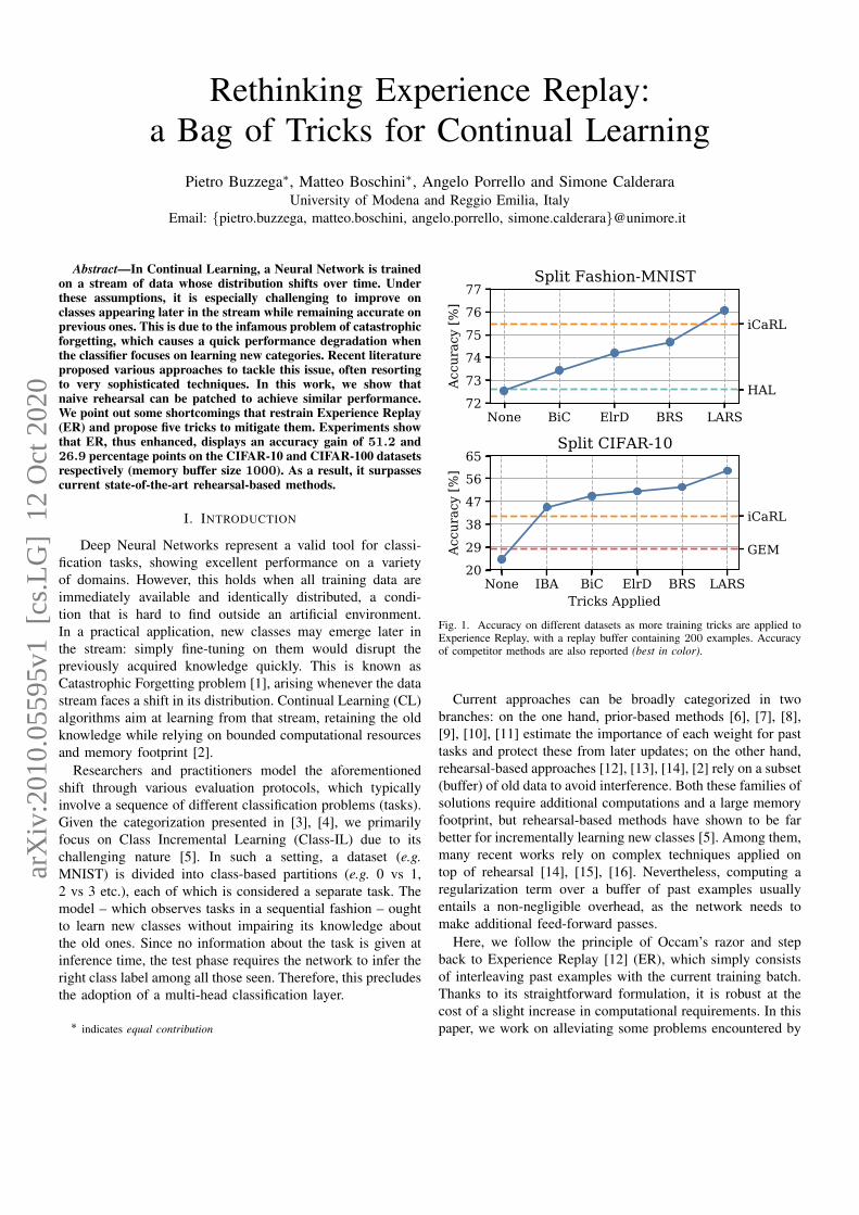
Fig. 1. Accuracy on different datasets as more training tricks are applied toExperience Replay, with a replay buffer containing 200 examples. Accuracyof competitor methods are also reported (best in color).

Current approaches can be broadly categorized in twobranches: on the one hand, prior-based methods [6], [7], [8],[9], [10], [11] estimate the importance of each weight for pasttasks and protect these from later updates; on the other hand,rehearsal-based approaches [12], [13], [14], [2] rely on a subset(buffer) of old data to avoid interference. Both these families ofsolutions require additional computations and a large memoryfootprint, but rehearsal-based methods have shown to be farbetter for incrementally learning new classes [5]. Among them,many recent works rely on complex techniques applied ontop of rehearsal [14], [15], [16]. Nevertheless, computing aregularization term over a buffer of past examples usuallyentails a non-negligible overhead, as the network needs tomake additional feed-forward passes.

Here, we follow the principle of Occam’s razor and stepback to Experience Replay [12] (ER), which simply consistsof interleaving past examples with the current training batch.Thanks to its straightforward formulation, it is robust at thecost of a slight increase in computational requirements. In thispaper, we work on alleviating some problems encountered by

arX

iv:2

010.

0559

5v1

[cs

.LG

] 1

2 O

ct 2

020

naive replay in the Class-IL setting. In more detail, we addressthe following issues:(a) Rehearsal methods could experience overfitting, as they

repeatedly optimize the examples stored in a relativelysmall buffer2;

(b) Incrementally learning a sequence of classes implicitlybiases the network towards newer ones, making theperformance unbalanced in favor of the latest task en-countered [17], [18];

(c) The memory buffer is commonly populated by samplingrandom items from the training stream, with the aim ofobtaining an i.i.d. distribution [14], [19]. While this isgenerally valid, there are failure cases. As an example, itmay leave out some classes when the buffer is small.

We illustrate how few modifications (a bag of tricks) notonly mitigate the above-mentioned issues, but also make thesimplest rehearsal baseline outperform the SOTA. Our maincontributions are:• a collection of five modifications that can be easily

applied to CL methods to improve their performance;• experiments showing that ER – when equipped with

these tricks – outperforms state-of-the-art rehearsal meth-ods on four distinct Class-IL experimental settings, thusproviding a new reliable baseline for any practitionerapproaching Continual Learning;

• further analysis clarifying how the tricks affect the accu-racy of ER and their applicability to other methods.

In light of the remarkable increase in performance that resultsfrom the application of our proposed tricks, we hope that thiswork will constitute a valuable quick reference as well as astepping stone for the design of more accurate CL approaches.

II. RELATED WORKS

After the first formulation of catastrophic forgetting inANNs [1], early works dating back to the 1990s [12], [20]proposed a straightforward solution to it, that is storing previ-ously seen examples in a memory buffer and later interleavingthem with new training batches. We refer the reader to Sec. IIIfor a detailed description of this simple, yet still very effectivemethod, generally known as Experience Replay (ER).

In the 2010s, the advent of Deep Neural Networks sparkedrenewed interest in Continual Learning [21] leading to a veryprolific production of works trying to counter forgetting. Thesecontributions can be split into two categories: those that storeparameters and those that store past examples.

The first group encompasses all methods that save pastnetwork configurations to prevent drifting away from them.In [9], Rusu et al. delegate distinct tasks to distinct neuralnetworks, limiting interference by design. Although this isa very effective strategy, it must be noted that the cost forstoring entire new models is very high (it grows linearly w.r.t.the number of tasks). [10], [11], [22] also suggest similarapproaches that adapt the model’s architecture to multi-task

2An early-sampled item in the Split CIFAR-10 protocol (buffer size 500;replay batch size 32) is replayed approximately 5000 times.

settings. Alternatively, [23], [6], [7], [8], [17], [18] keep amodel checkpoint and use it to formulate an additional lossterm to prevent excessive weight alterations in later tasks.

On the opposite side of the spectrum, methods storing pastexamples relate to ER, in that they also tackle forgetting bycollecting exemplars seen in previous training phases. Rebuffiet al. propose iCaRL [2], an approach that classifies newexemplars by finding the nearest mean representation of pastelements in an incrementally learned feature space. GEM [13]and its more efficient version A-GEM [24] showcase anothernon-obvious use of memories, as they define inequality con-straints to avoid the increase in the losses w.r.t. previous taskswhile allowing for their decrease.

Although – quite remarkably – none of the mentionedpapers draw any experimental comparison with it, ExperienceReplay still appears to be a strong solution to catastrophicforgetting. This is corroborated by a line of very recentworks [14], [19], [15], [16], [25], [26], [27] that argue forits superior effectiveness in comparison to other methods andpropose various extensions to it. Meta-Experience Replay [14]notably complements replay with meta-learning techniquesto maximize transfer and minimize interference. The authorsof [15] propose an optimized strategy for choosing what tostore in the memory buffer, while [16] explores an alternativepolicy for sampling from it. On the other hand, [25] suggestsadopting a Variational Autoencoder as a compression mecha-nism to maximize the efficiency of storing replay exemplars.Most recently, HAL [26] equips ER with a regularization termanchoring the network’s responses towards data-points learnedfrom classes of previous tasks and DER [27] shows that simplyreplaying network responses instead of ground truth labelsproduces an even stronger baseline than ER.

It is also worth mentioning that other works [28], [29]exploit generative models in place of the memory buffer. Onthe one hand, this favorably allows sampling data-points fromthe distributions underlying the old tasks. On the other hand,it requires training the generator online, thus giving rise to achicken and egg problem. Furthermore, as [28] regards ER asan upper bound for the proposed method, it appears that theformer is currently a more effective and viable solution.

In the light of these considerations, we set out to provethat ER can perform significantly better than other approacheswhen equipped with the tricks described in Sec. IV.

III. BASELINE METHOD

A Class Incremental classification problem requires traininga learner fθ to classify samples x that belong to one class yout of a given dataset D. This corresponds to minimizing thefollowing loss term:

L = E(x,y)∼D[`(y, fθ(x))

]. (1)

In a CL scenario, the dataset is divided into Nt tasks, duringeach of which t ∈ {1, ..., Nt} only examples belonging to aspecific partition of classes Dt are shown. As the classifieronly observes one portion of the dataset at a time, it cannotoptimize Eq. 1 directly. Therefore, it must devise a strategy

ModelData

Aug.𝒙 𝒙𝒂𝒖𝒈

Memory

Buffer𝒙𝒂𝒖𝒈𝒙𝒂𝒖𝒈𝒙𝒂𝒖𝒈

store

train

rehearse

𝒙𝒂𝒖𝒈𝒙𝒂𝒖𝒈𝒙𝒂𝒖𝒈

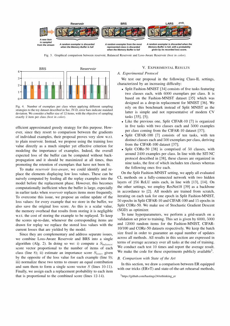
A new item

is sampled

from the stream A random exemplar is discarded

when the Memory Buffer is full

Reservoir

A random exemplar from the most

represented class is discarded

when the Memory Buffer is full

BRS

A random exemplar is discarded when the

Memory Buffer is full, with a probability

given by its recorded loss score.

LARS

Data

Aug.𝒙 Model𝒙𝒂𝒖𝒈

Memory

Buffer

𝒙𝒂𝒖𝒙

train

rehearse

storeData

Aug.𝒙𝒂𝒖𝒈𝒙𝒂𝒖𝒈𝒙𝒂𝒖𝒈′

prob.

Model

Data

Aug.

𝒙

Memory

Buffer

store

train

rehearse

𝒙

train

rehearse

store

Data

Aug.

Data

Aug.

𝒙Memory

Buffer

Model

Reservoir LARS prob.BRS

𝒙Input

Stream

Memory

Buffer

Cross-

Entropy

Loss

𝒙𝒂𝒖𝒙𝒓

store

examples

store

responses

MSE

Loss

Model

𝒚

𝒙𝒚

𝒙𝒚

𝒙𝒚

𝒙𝒚

𝒙𝒚

𝒙𝒚

𝒙𝒚

… …

Input

stream

Output

logits

𝒙Input

Stream

Memory

Buffer

Cross-

Entropy

Loss

store

examples

and labels

store

responses

MSE

and CE

Losses

Model

𝒚

𝒚

𝒙𝒂𝒖

𝒚

𝒙𝒓

𝒚

𝒙𝒂𝒖𝒈𝒙𝒂𝒖𝒈𝒙𝒂𝒖𝒈𝒙𝒂𝒖𝒈

𝒙𝒂𝒖𝒈𝒙𝒂𝒖𝒈𝒙𝒂𝒖𝒈

𝒙𝒂𝒖𝒈𝒙𝒂𝒖𝒈

𝒙𝒂𝒖𝒈′𝒙𝒂𝒖𝒈′𝒙𝒂𝒖𝒈′

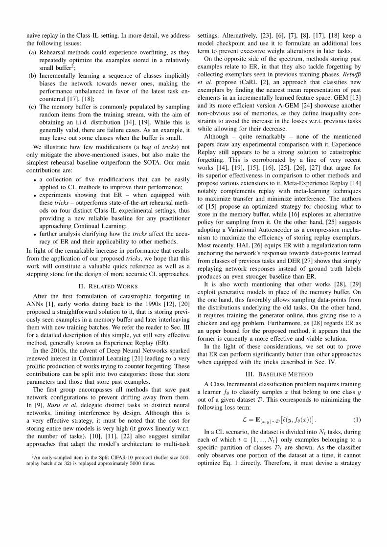
(a) (b)Fig. 2. Graphical comparison between rehearsal on augmented examples (a)and Independent Buffer Augmentation (b) (best in color).

to approximate it. Experience Replay addresses this issueby storing exemplars and labels from previous tasks in areplay buffer B. During each training step, it merges some ofthese items with the current batch: consequently, the networkrehearses past tasks as it learns current data. This amounts tooptimizing the following loss term as a surrogate of Eq. 1:

L′ = E(x,y)∼Dt

[`(y, fθ(x))

]+ E(x,y)∼B

[`(y, fθ(x))

]. (2)

This practical solution only introduces two additional hyper-parameters to fθ, namely the replay buffer size |B| and thenumber of elements that we draw from it at each step. Inthis work, we initially assume to update the buffer with thereservoir sampling strategy [30] (see Alg. 1), as proposedin [14]. This guarantees that each input exemplar has thesame probability |B|/|D| of entering the replay buffer. Weprefer this solution both to herding [2] and the class-wiseFIFO [19] strategies (a.k.a. ring buffer). Unlike reservoir, theformer needs to retain the entire training set of each task.Conversely, the latter does not exploit the whole memory andis more likely to overfit (as pointed out in [19]).

IV. TRAINING TRICKS

In this section, we discuss some issues that ER encountersin the Class-IL setting and propose effective tricks to mitigatethem. On the one hand, Sec. IV-A, IV-D and IV-E describeimprovements to the replay buffer and can, therefore, easilyextend to other rehearsal-based methods. On the other hand,the tricks described in Sec. IV-B and IV-C are more generaland applicable to any Class-IL method.

A. Independent Buffer Augmentation (IBA)

Data augmentation is an effective strategy for improvingthe generalization capabilities of a Deep Network [31]. Whendealing with Continual Learning scenarios, one can apply dataaugmentation on the input stream of data (i.e. the examplesshown to the net during each task). However, for a rehearsalmethod, replayed exemplars constitute a significant portionof the overall training input. This could pose a serious risk

of overfitting the memory buffer, which we address throughIndependent Buffer Augmentation (IBA): in addition to theregular augmentation performed on the input stream, we storeexamples not augmented in the memory buffer; this way, wecan augment them independently when drawn for later replay.By so doing, we minimize overfitting on the memory andintroduce additional variety in the rehearsal examples.

While adopting this simple expedient could seem a no-brainer, its application in literature should not be taken forgranted. As an example, the CL methods implemented in thecodebase of [13]3 and [15]4 store the augmented examples inthe memory buffer and re-use them as-they-are, as illustratedin Fig. 2(a). On the contrary, we remark that it is much morebeneficial to show the model replay examples that undergodistinct transformations, as shown in Fig. 2(b).

B. Bias Control (BiC)

Given the sequential nature of the Class-IL setting, thenetwork’s predictions end up showing bias towards the currenttask. Indeed, a single-head classifier is less prone to predictingclasses found in prior tasks than those learned just beforetesting. Such bias is linked to the whole model and notexclusively to its final classification layer: consequently, thetrivial solution of zeroing the latter is not beneficial.

This imbalance problem is analyzed by both Hou et al.in [18] and Wu et al. in [17]. The former addresses this issuestructurally by devising a specific margin-ranking loss termaimed keeping representations from different tasks separated.However, the latter work proposes a much simpler and modularsolution, which we also apply here: the addition of a simpleBias Correction Layer to the model. This layer consists in alinear model with two parameters α and β that compensatesthe kth output logit ok as follows.

qk =

{α · ok + β if k was trained in the last taskok otherwise

(3)

Such a layer is applied downstream of the classifier to yieldthe final output at test time. Thanks to its small size, it canbe easily trained at the end of each task by leveraging alimited amount of exemplars. Importantly, while [17] employsa separate validation set for this purpose, we simply exploit thesame replay buffer we use for rehearsal methods. Parameters αand β are optimized through the cross-entropy loss, as follows:

`BiC = −∑k

δy=k log[softmax(qk)]. (4)

We agree with the authors of [17] on the effectiveness ofthis simple linear model to counter the above-mentioned bias.

C. Exponential LR Decay (ELRD)

Arguably, the best way to preserve previous knowledgeis not to learn anything new. To this aim, we propose todecrease the learning rate progressively at each iteration; we

3https://github.com/facebookresearch/GradientEpisodicMemory4https://github.com/rahafaljundi/Gradient-based-Sample-Selection

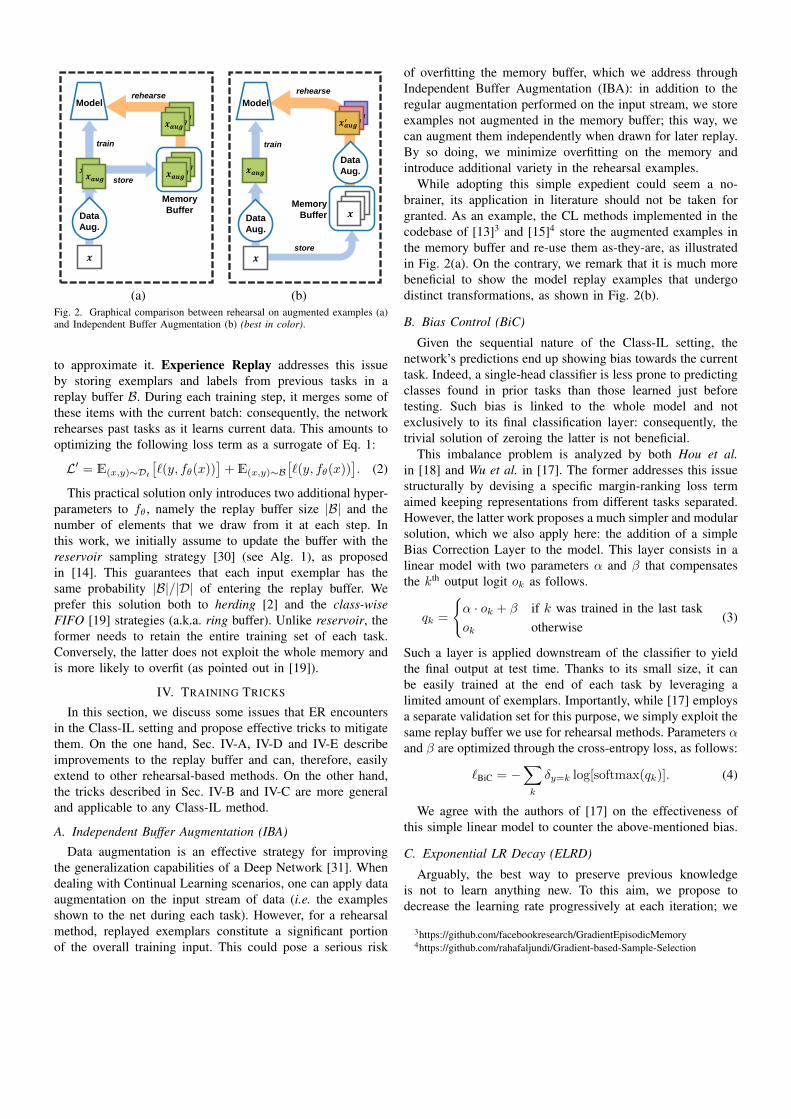
Algorithm 1 Balanced Reservoir Sampling1: Input: exemplar (x, y), replay buffer B,2: number of seen examples N .3: if |B| > N then4: B[N ]← (x, y)5: else6: j ← RandInt([0, N ])7: if j < |B| then

8: B[j]← (x, y)

Reservoir Sampling

9: y ← argmax ClassCounts(B, y)10: k ← RandChoice({k;B[k] = (x, y), y = y})11: B[k]← (x, y)

Balanced Reservoir Sampling

12: end if13: end if

found exponential decay particularly effective. Exponential-based rules for decaying the learning rate were early intro-duced in literature to speed up the learning process [32],[33]. CL algorithms that exploit this technique [6], [2] do soin a task-wise manner (namely, the schedule starts again atthe beginning of each task). Differently, we point out thatdecreasing the learning rate for the whole duration of thetraining relieves catastrophic forgetting. We thus recommendto compute the learning rate for the jth example as follows:

lrj = lr0 · γNex , (5)

where Nex is the number of input examples seen so far, lr0indicates the initial learning rate for training and γ is a hyper-parameter tuned to make the learning rate approximately 1/6of the initial value at the end of the training.

It is worth noting that decreasing the learning rate yieldsan additional regularization objective, which penalizes weightschange between subsequent steps. In Continual Learning, afamily of non-rehearsal approaches [6], [7], [8] rely on thisconcept, applying a loss term to prevent the same kind ofinterference. However, ELrD does not produce the additionaloverhead that characterizes these methods.

D. Balanced Reservoir Sampling (BRS)

Reservoir sampling is an online update procedure thatpopulates a fixed-size buffer with data coming from a stream.It guarantees each exemplar from that stream to be representedin the buffer with the same probability |B|/i at any iteration i,which makes it equivalent to an offline random sampling ateach time step. However, if the dataset D contains exemplarsfrom C distinct classes and we randomly sample |B| of them,the probability of leaving at least one class out is given by:

P =

(1− 1

C

)|B|. (6)

This would result in leaving 1/P classes out of B, whichbecomes especially critical when dealing with small buffers:

Algorithm 2 Loss-Aware Balanced Reservoir Sampling1: Input: exemplar (x, y, `), replay buffer B,2: number of seen examples N .3: if |B| > N then4: B[N ]← (x, y, `)5: else6: j ← RandInt([0, N ])7: if j < |B| then8: Sbalance ← {ClassCounts(y); ∀(x, y, `) ∈ B}9: Sloss ← {−`;∀(x, y, `) ∈ B}

10: α←∑k |Sbalance[k]|/

∑k |Sloss[k]|

11: S ← Sloss · α+ Sbalance

12: probs← S/∑k S[k]

13: k ← RandInt([0, |B|],probs)14: B[k]← (x, y, `)15: end if16: end if

considering |B| ≈ C, that probability increases from 0.25 forC = 2 to ≈ 0.367 for C →∞ (e.g. 0.349 for C = 10).

To overcome such an issue, other approaches resort to thering buffer [19] or the herding [2] strategy; however, these arenot optimal in terms of buffer exploitation or computationaloverhead. The former reserves a slice as large as |B|/C foreach class: since classes are shown incrementally, this wouldleave the main part of the buffer empty. The latter changesthe dimension of such slices with the number of seen classes,always reserving |B|/Cseen slots for each class (where Cseenindicates the number of seen classes). Despite its increasedefficiency in terms of memory, herding additionally performsa forward pass over the training set at the end of each task.

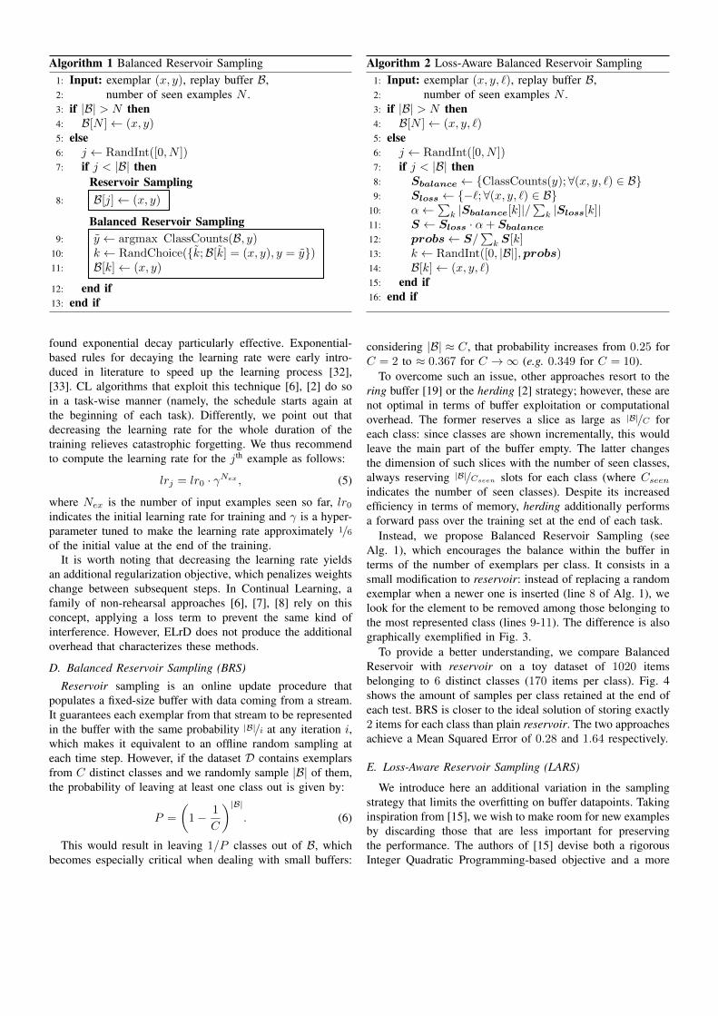
Instead, we propose Balanced Reservoir Sampling (seeAlg. 1), which encourages the balance within the buffer interms of the number of exemplars per class. It consists in asmall modification to reservoir: instead of replacing a randomexemplar when a newer one is inserted (line 8 of Alg. 1), welook for the element to be removed among those belonging tothe most represented class (lines 9-11). The difference is alsographically exemplified in Fig. 3.

To provide a better understanding, we compare BalancedReservoir with reservoir on a toy dataset of 1020 itemsbelonging to 6 distinct classes (170 items per class). Fig. 4shows the amount of samples per class retained at the end ofeach test. BRS is closer to the ideal solution of storing exactly2 items for each class than plain reservoir. The two approachesachieve a Mean Squared Error of 0.28 and 1.64 respectively.

E. Loss-Aware Reservoir Sampling (LARS)

We introduce here an additional variation in the samplingstrategy that limits the overfitting on buffer datapoints. Takinginspiration from [15], we wish to make room for new examplesby discarding those that are less important for preservingthe performance. The authors of [15] devise both a rigorousInteger Quadratic Programming-based objective and a more

ModelData

Aug.𝒙 𝒙𝒂𝒖𝒈

Memory

Buffer𝒙𝒂𝒖𝒈𝒙𝒂𝒖𝒈𝒙𝒂𝒖𝒈

store

train

rehearse

𝒙𝒂𝒖𝒈𝒙𝒂𝒖𝒈𝒙𝒂𝒖𝒈

A new item

is sampled

from the stream A random exemplar is discarded

when the Memory Buffer is full

Reservoir

A random exemplar from the most

represented class is discarded

when the Memory Buffer is full

BRS

A random exemplar is discarded when the

Memory Buffer is full, with a probability

given by its recorded loss score.

LARS

Data

Aug.𝒙 Model𝒙𝒂𝒖𝒈

Memory

Buffer

𝒙𝒂𝒖𝒙

train

rehearse

storeData

Aug.𝒙𝒂𝒖𝒈𝒙𝒂𝒖𝒈𝒙𝒂𝒖𝒈′

prob.

Model

Data

Aug.

𝒙

𝒙𝒂𝒖𝒈

Memory

Buffer

store

train

rehearse

𝒙𝒂𝒖𝒈𝒙𝒂𝒖𝒈𝒙𝒂𝒖𝒈

𝒙𝒂𝒖𝒈𝒙𝒂𝒖𝒈𝒙𝒂𝒖𝒈

𝒙

𝒙𝒂𝒖𝒙

train

rehearse

store

𝒙𝒂𝒖𝒈𝒙𝒂𝒖𝒈𝒙𝒂𝒖𝒈′

Data

Aug.

Data

Aug. Memory

Buffer

Model

𝒙𝒂𝒖𝒈

Fig. 3. Graphical comparison between reservoir, Balanced Reservoir and Loss-Aware Reservoir (best in color).

0

1

2

3

4BRS Reservoir

Fig. 4. Number of exemplars per class when applying different samplingstrategies to the toy dataset described in Sec. IV-D, error bars indicate standarddeviation. We consider a buffer size of 12 items, with the objective of samplingexactly 2 item per class (best in color).

efficient approximated greedy strategy for this purpose. How-ever, since they resort to comparison between the gradientsof individual examples, their proposal proves very slow w.r.t.to plain reservoir. Instead, we propose using the training lossvalue directly as a much simpler yet effective criterion formodeling the importance of examples. Indeed, the overallexpected loss of the buffer can be computed without back-propagation and it should be maximized at all times, thuspromoting the retention of exemplars that have not been fit.

To make reservoir loss-aware, we could identify and re-place the elements displaying low loss values. These can benaively computed by feeding all the replay examples into themodel before the replacement phase. However, this becomescomputationally inefficient when the buffer is large, especiallyin earlier tasks when reservoir replaces items more frequently.To overcome this issue, we propose an online update of theloss values: for every example that we store in the buffer, wealso save the original loss score. As this is a scalar value,the memory overhead that results from storing it is negligiblew.r.t. the cost of storing the example to be replayed. To keepthe scores up-to-date, whenever the corresponding items aredrawn for replay we replace the stored loss values with thecurrent losses that are yielded by the model.

Since they are complementary and address separate issues,we combine Loss-Aware Reservoir and BRS into a singlealgorithm (Alg. 2). In doing so we: i) compute a Sbalancescore vector proportional to the number of items of eachclass (line 8); ii) estimate an importance score Sloss, givenby the opposite of the loss value for each example (line 9);iii) normalize these two terms to ensure an equal contributionand sum them to form a single score vector S (lines 10-11).Finally, we assign each a replacement probability to each itemthat is proportional to the combined score (lines 12-14).

V. EXPERIMENTAL RESULTS

A. Experimental Protocol

We test our proposal in the following Class-IL settings,characterized by an increasing difficulty:• Split Fashion-MNIST [34] consists of five tasks featuring

two classes each, with 6000 exemplars per class. It isbased on the Fashion-MNIST dataset [35] which wasdesigned as a drop-in replacement for MNIST [36]. Werely on this benchmark instead of Split MNIST as thelatter is simple and not representative of modern CVtasks [35], [5];

• Like the previous one, Split CIFAR-10 [7] is organizedin five tasks with two classes each and 5000 examplesper class coming from the CIFAR-10 dataset [37];

• Split CIFAR-100 [7] consists of ten tasks, with tendistinct classes each and 500 exemplars per class, derivingfrom the CIFAR-100 dataset [37];

• Split CORe-50 [38] is comprised of 50 classes, witharound 2400 examples per class. In line with the SIT-NCprotocol described in [38], these classes are organized innine tasks, the first of which includes ten classes whereasthe following ones five each.

On the Split Fashion-MNIST setting, we apply all evaluatedCL methods on a fully-connected network with two hiddenlayers of 256 ReLU units each, in line with [13], [14]. Onthe other settings, we employ ResNet18 [39] as a backbonein accordance to [2]. All models are trained from scratch,iterating on each task for one epoch in Split Fashion-MNIST,50 epochs in Split CIFAR-10 and CIFAR-100 and 15 epochs inSplit CORe-50. We make use of Stochastic Gradient Descent(SGD) as optimizer.

To tune hyperparameters, we perform a grid-search on avalidation set prior to training. This set is given by 6000, 5000and 12000 random items for the Fashion-MNIST, CIFAR-10/100 and CORe-50 datasets respectively. We keep the batchsize fixed in order to guarantee an equal number of updatesacross all methods. All results in this section are expressed interms of average accuracy over all tasks at the end of training.We conduct each test 10 times and report the average result.We make the code for these experiments publicly available5.

B. Comparison with State of the Art

In this section, we draw a comparison between ER equippedwith our tricks (ER+T) and state-of-the-art rehearsal methods,

5https://github.com/hastings24/rethinking er

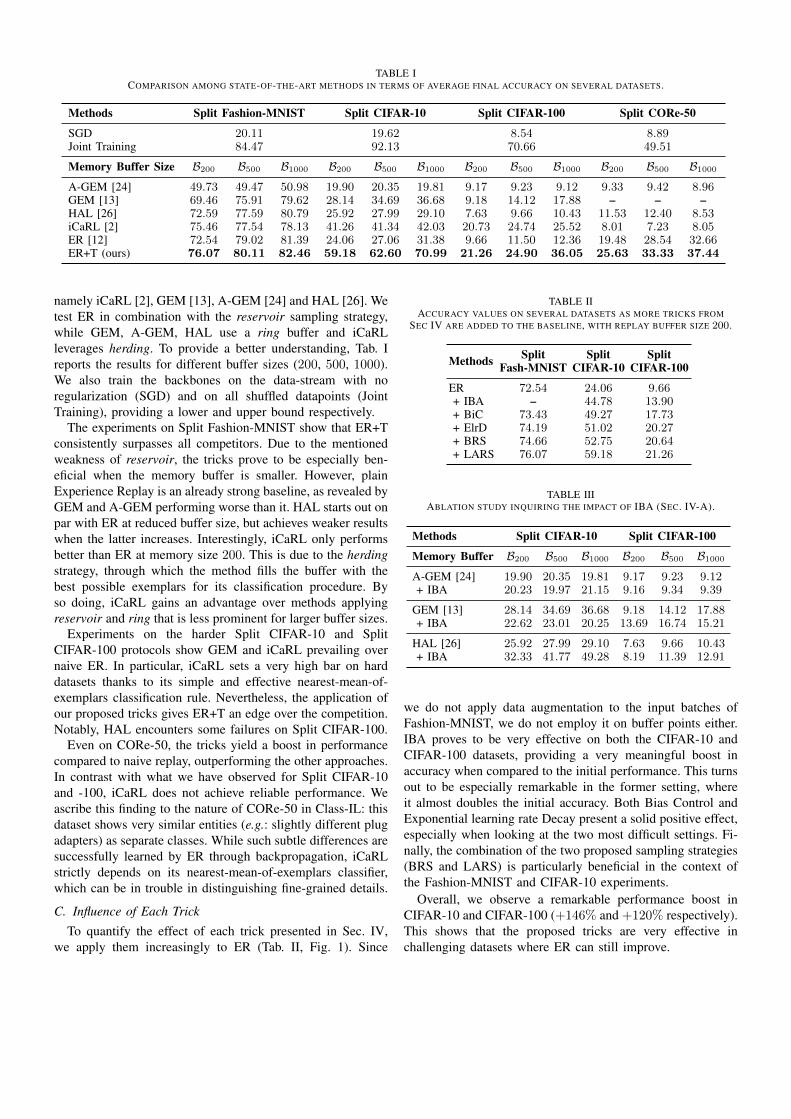
TABLE ICOMPARISON AMONG STATE-OF-THE-ART METHODS IN TERMS OF AVERAGE FINAL ACCURACY ON SEVERAL DATASETS.

Methods Split Fashion-MNIST Split CIFAR-10 Split CIFAR-100 Split CORe-50

SGD 20.11 19.62 8.54 8.89Joint Training 84.47 92.13 70.66 49.51

Memory Buffer Size B200 B500 B1000 B200 B500 B1000 B200 B500 B1000 B200 B500 B1000

A-GEM [24] 49.73 49.47 50.98 19.90 20.35 19.81 9.17 9.23 9.12 9.33 9.42 8.96GEM [13] 69.46 75.91 79.62 28.14 34.69 36.68 9.18 14.12 17.88 – – –HAL [26] 72.59 77.59 80.79 25.92 27.99 29.10 7.63 9.66 10.43 11.53 12.40 8.53iCaRL [2] 75.46 77.54 78.13 41.26 41.34 42.03 20.73 24.74 25.52 8.01 7.23 8.05ER [12] 72.54 79.02 81.39 24.06 27.06 31.38 9.66 11.50 12.36 19.48 28.54 32.66ER+T (ours) 76.07 80.11 82.46 59.18 62.60 70.99 21.26 24.90 36.05 25.63 33.33 37.44

namely iCaRL [2], GEM [13], A-GEM [24] and HAL [26]. Wetest ER in combination with the reservoir sampling strategy,while GEM, A-GEM, HAL use a ring buffer and iCaRLleverages herding. To provide a better understanding, Tab. Ireports the results for different buffer sizes (200, 500, 1000).We also train the backbones on the data-stream with noregularization (SGD) and on all shuffled datapoints (JointTraining), providing a lower and upper bound respectively.

The experiments on Split Fashion-MNIST show that ER+Tconsistently surpasses all competitors. Due to the mentionedweakness of reservoir, the tricks prove to be especially ben-eficial when the memory buffer is smaller. However, plainExperience Replay is an already strong baseline, as revealed byGEM and A-GEM performing worse than it. HAL starts out onpar with ER at reduced buffer size, but achieves weaker resultswhen the latter increases. Interestingly, iCaRL only performsbetter than ER at memory size 200. This is due to the herdingstrategy, through which the method fills the buffer with thebest possible exemplars for its classification procedure. Byso doing, iCaRL gains an advantage over methods applyingreservoir and ring that is less prominent for larger buffer sizes.

Experiments on the harder Split CIFAR-10 and SplitCIFAR-100 protocols show GEM and iCaRL prevailing overnaive ER. In particular, iCaRL sets a very high bar on harddatasets thanks to its simple and effective nearest-mean-of-exemplars classification rule. Nevertheless, the application ofour proposed tricks gives ER+T an edge over the competition.Notably, HAL encounters some failures on Split CIFAR-100.

Even on CORe-50, the tricks yield a boost in performancecompared to naive replay, outperforming the other approaches.In contrast with what we have observed for Split CIFAR-10and -100, iCaRL does not achieve reliable performance. Weascribe this finding to the nature of CORe-50 in Class-IL: thisdataset shows very similar entities (e.g.: slightly different plugadapters) as separate classes. While such subtle differences aresuccessfully learned by ER through backpropagation, iCaRLstrictly depends on its nearest-mean-of-exemplars classifier,which can be in trouble in distinguishing fine-grained details.

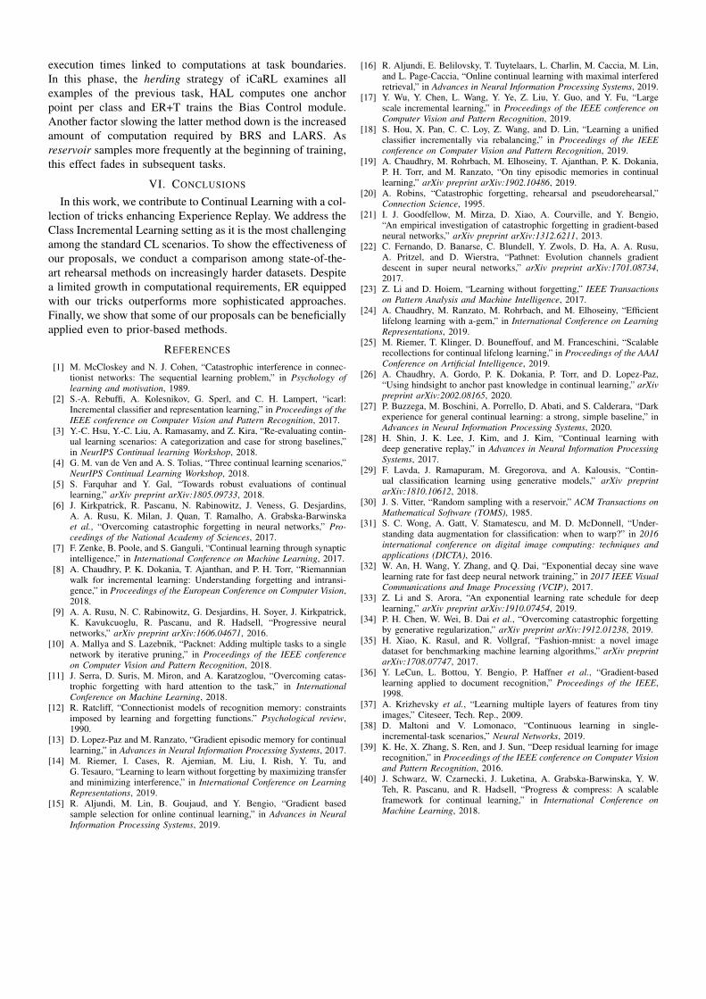
C. Influence of Each Trick

To quantify the effect of each trick presented in Sec. IV,we apply them increasingly to ER (Tab. II, Fig. 1). Since

TABLE IIACCURACY VALUES ON SEVERAL DATASETS AS MORE TRICKS FROM

SEC IV ARE ADDED TO THE BASELINE, WITH REPLAY BUFFER SIZE 200.

Methods Split Split SplitFash-MNIST CIFAR-10 CIFAR-100

ER 72.54 24.06 9.66+ IBA – 44.78 13.90+ BiC 73.43 49.27 17.73+ ElrD 74.19 51.02 20.27+ BRS 74.66 52.75 20.64+ LARS 76.07 59.18 21.26

TABLE IIIABLATION STUDY INQUIRING THE IMPACT OF IBA (SEC. IV-A).

Methods Split CIFAR-10 Split CIFAR-100

Memory Buffer B200 B500 B1000 B200 B500 B1000

A-GEM [24] 19.90 20.35 19.81 9.17 9.23 9.12+ IBA 20.23 19.97 21.15 9.16 9.34 9.39

GEM [13] 28.14 34.69 36.68 9.18 14.12 17.88+ IBA 22.62 23.01 20.25 13.69 16.74 15.21

HAL [26] 25.92 27.99 29.10 7.63 9.66 10.43+ IBA 32.33 41.77 49.28 8.19 11.39 12.91

we do not apply data augmentation to the input batches ofFashion-MNIST, we do not employ it on buffer points either.IBA proves to be very effective on both the CIFAR-10 andCIFAR-100 datasets, providing a very meaningful boost inaccuracy when compared to the initial performance. This turnsout to be especially remarkable in the former setting, whereit almost doubles the initial accuracy. Both Bias Control andExponential learning rate Decay present a solid positive effect,especially when looking at the two most difficult settings. Fi-nally, the combination of the two proposed sampling strategies(BRS and LARS) is particularly beneficial in the context ofthe Fashion-MNIST and CIFAR-10 experiments.

Overall, we observe a remarkable performance boost inCIFAR-10 and CIFAR-100 (+146% and +120% respectively).This shows that the proposed tricks are very effective inchallenging datasets where ER can still improve.

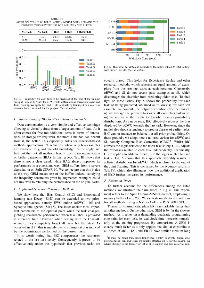
TABLE IVACCURACY VALUES ON SPLIT FASHION-MNIST WHEN APPLYING THE

PROPOSED TRICKS BY THE USE OF A 500-EXAMPLES BUFFER.

Methods No trick BiC CBiC CBiC+ElrD

SI 19.91 24.67 33.15 35.51oEWC 20.04 25.71 40.36 43.85

oEWC oEWC+BiC

oEWC+CBiC

JointTraining

0.0

0.2

0.4

0.6

0.8

1.0

Task

Pro

babi

lity

Task 1Task 2Task 3Task 4Task 5

Fig. 5. Probability for each task to be predicted at the end of the trainingon Split Fashion-MNIST, for oEWC with different bias correction layers andJoint Training. We apply BiC and CBiC to oEWC by training it on a reservoirmemory buffer included for the purpose (best in color).

D. Applicability of IBA to other rehearsal methods

Data augmentation is a very simple and effective techniqueallowing to virtually draw from a larger amount of data. As itoften comes for free (no additional costs in terms of annota-tions or storage are required), the more a method can benefitfrom it, the better. This especially holds for rehearsal-basedmethods approaching CL scenarios, where only few examplesare available to guard the old knowledge. Surprisingly, wefind out that not all methods benefit from data-augmentationon buffer datapoints (IBA). In this respect, Tab. III shows thatthere is not a clear trend: while HAL always improves itsperformance in a consistent way, GEM suffers from a severedegradation on Split CIFAR-10. We conjecture that this is dueto the way GEM makes use of the buffer: indeed, satisfyingthe inequality constraints given by augmented examples couldnot link well to retaining the performance on the original tasks.

E. Applicability to non-Rehearsal Methods

We show here that Bias Control (BiC) and Exponentiallearning rate Decay (ElrD) can be extended to two prior-based approaches, namely EWC online (oEWC) [40] andSynaptic Intelligence (SI) [7]. The latter anchor most impor-tant parameters at the optimal point when the task changes,yielding remarkable performance when task-label is providedat inference time. However, when dealing with the Class-ILscenario, they completely forget all tasks but the latest. Asobserved in [17], this is mainly due to an implicit bias inducedby the optimization performed on the current task.

It is worth noting that BiC compensates the responsesrelated to the last task solely. Consequently, it proves to beeffective only under the hypothesis that previous tasks are

0 30 60 90 120 150Wallclock Time (secs)

ER

A-GEM

iCaRL

ER+T

HAL

GEM

Task 1Task 2Task 3Task 4Task 5

Fig. 6. Run times for different methods on the Split Fashion-MNIST setting,with buffer size 200 (best in color).

equally biased. This holds for Experience Replay and otherrehearsal methods, which rehearse an equal amount of exem-plars from the previous tasks at each iteration. Conversely,oEWC and SI do not access past examples at all, whichdiscourages the classifier from predicting older tasks. To shedlight on these issues, Fig. 5 shows the probability for eachtask of being predicted, obtained as follows: i) for each testexample, we compute the output distribution over the classes;ii) we average the probabilities over all exemplars task-wise;iii) we normalize the results to describe them as probabilitydistributions. As can be seen, BiC effectively reduces the biasdisplayed by oEWC towards the last task. However, since themodel also shows a tendency to predict classes of earlier tasks,BiC cannot manage to balance out all prior probabilities. Onthese grounds, we adopt here a tailored variant for oEWC andSI, namely Complete Bias Correction (CBiC)6. Whilst BiCcorrects the logits related to the latest task solely, CBiC adjuststhe responses related to each task independently. Technically,CBiC applies an additive offset βt to the logits related to eachtask t. Fig. 5 shows that this approach favorably results ina flatter distribution for oEWC, which is closer to the one ofthe Joint Training. This is confirmed by the accuracy results inTab. IV, which also illustrates how the additional applicationof ElrD further increases its performance.

F. Execution Times

To further account for the differences among the listedmethods, we illustrate their run times in Fig. 6. This experi-ment refers to the Split Fashion-MNIST dataset, employing amemory buffer of size 200. We ran tests on identical conditionsfor all methods, using a NVidia GeForce RTX 2080 GPU.

Thanks to its simplicity, plain ER is remarkably faster thanall other methods. On the other side, GEM is by far the slowestmethod. As it relies on a demanding quadratic programmingconstraint for each task, its wallclock time increases remark-ably as the training progresses. By comparison, A-GEM isclearly much faster as it only applies one similar constraint atall times. iCaRL, HAL and ER+T have similar medium-long

6It must be noted that, since Experience Replay is evenly biased w.r.t.previous tasks, BiC and CBiC are equally effective on it. For this reason, weadvise sticking to the former for ER as it is simpler and thus easier to train.

execution times linked to computations at task boundaries.In this phase, the herding strategy of iCaRL examines allexamples of the previous task, HAL computes one anchorpoint per class and ER+T trains the Bias Control module.Another factor slowing the latter method down is the increasedamount of computation required by BRS and LARS. Asreservoir samples more frequently at the beginning of training,this effect fades in subsequent tasks.

VI. CONCLUSIONS

In this work, we contribute to Continual Learning with a col-lection of tricks enhancing Experience Replay. We address theClass Incremental Learning setting as it is the most challengingamong the standard CL scenarios. To show the effectiveness ofour proposals, we conduct a comparison among state-of-the-art rehearsal methods on increasingly harder datasets. Despitea limited growth in computational requirements, ER equippedwith our tricks outperforms more sophisticated approaches.Finally, we show that some of our proposals can be beneficiallyapplied even to prior-based methods.

REFERENCES

[1] M. McCloskey and N. J. Cohen, “Catastrophic interference in connec-tionist networks: The sequential learning problem,” in Psychology oflearning and motivation, 1989.

[2] S.-A. Rebuffi, A. Kolesnikov, G. Sperl, and C. H. Lampert, “icarl:Incremental classifier and representation learning,” in Proceedings of theIEEE conference on Computer Vision and Pattern Recognition, 2017.

[3] Y.-C. Hsu, Y.-C. Liu, A. Ramasamy, and Z. Kira, “Re-evaluating contin-ual learning scenarios: A categorization and case for strong baselines,”in NeurIPS Continual learning Workshop, 2018.

[4] G. M. van de Ven and A. S. Tolias, “Three continual learning scenarios,”NeurIPS Continual Learning Workshop, 2018.

[5] S. Farquhar and Y. Gal, “Towards robust evaluations of continuallearning,” arXiv preprint arXiv:1805.09733, 2018.

[6] J. Kirkpatrick, R. Pascanu, N. Rabinowitz, J. Veness, G. Desjardins,A. A. Rusu, K. Milan, J. Quan, T. Ramalho, A. Grabska-Barwinskaet al., “Overcoming catastrophic forgetting in neural networks,” Pro-ceedings of the National Academy of Sciences, 2017.

[7] F. Zenke, B. Poole, and S. Ganguli, “Continual learning through synapticintelligence,” in International Conference on Machine Learning, 2017.

[8] A. Chaudhry, P. K. Dokania, T. Ajanthan, and P. H. Torr, “Riemannianwalk for incremental learning: Understanding forgetting and intransi-gence,” in Proceedings of the European Conference on Computer Vision,2018.

[9] A. A. Rusu, N. C. Rabinowitz, G. Desjardins, H. Soyer, J. Kirkpatrick,K. Kavukcuoglu, R. Pascanu, and R. Hadsell, “Progressive neuralnetworks,” arXiv preprint arXiv:1606.04671, 2016.

[10] A. Mallya and S. Lazebnik, “Packnet: Adding multiple tasks to a singlenetwork by iterative pruning,” in Proceedings of the IEEE conferenceon Computer Vision and Pattern Recognition, 2018.

[11] J. Serra, D. Suris, M. Miron, and A. Karatzoglou, “Overcoming catas-trophic forgetting with hard attention to the task,” in InternationalConference on Machine Learning, 2018.

[12] R. Ratcliff, “Connectionist models of recognition memory: constraintsimposed by learning and forgetting functions.” Psychological review,1990.

[13] D. Lopez-Paz and M. Ranzato, “Gradient episodic memory for continuallearning,” in Advances in Neural Information Processing Systems, 2017.

[14] M. Riemer, I. Cases, R. Ajemian, M. Liu, I. Rish, Y. Tu, andG. Tesauro, “Learning to learn without forgetting by maximizing transferand minimizing interference,” in International Conference on LearningRepresentations, 2019.

[15] R. Aljundi, M. Lin, B. Goujaud, and Y. Bengio, “Gradient basedsample selection for online continual learning,” in Advances in NeuralInformation Processing Systems, 2019.

[16] R. Aljundi, E. Belilovsky, T. Tuytelaars, L. Charlin, M. Caccia, M. Lin,and L. Page-Caccia, “Online continual learning with maximal interferedretrieval,” in Advances in Neural Information Processing Systems, 2019.

[17] Y. Wu, Y. Chen, L. Wang, Y. Ye, Z. Liu, Y. Guo, and Y. Fu, “Largescale incremental learning,” in Proceedings of the IEEE conference onComputer Vision and Pattern Recognition, 2019.

[18] S. Hou, X. Pan, C. C. Loy, Z. Wang, and D. Lin, “Learning a unifiedclassifier incrementally via rebalancing,” in Proceedings of the IEEEconference on Computer Vision and Pattern Recognition, 2019.

[19] A. Chaudhry, M. Rohrbach, M. Elhoseiny, T. Ajanthan, P. K. Dokania,P. H. Torr, and M. Ranzato, “On tiny episodic memories in continuallearning,” arXiv preprint arXiv:1902.10486, 2019.

[20] A. Robins, “Catastrophic forgetting, rehearsal and pseudorehearsal,”Connection Science, 1995.

[21] I. J. Goodfellow, M. Mirza, D. Xiao, A. Courville, and Y. Bengio,“An empirical investigation of catastrophic forgetting in gradient-basedneural networks,” arXiv preprint arXiv:1312.6211, 2013.

[22] C. Fernando, D. Banarse, C. Blundell, Y. Zwols, D. Ha, A. A. Rusu,A. Pritzel, and D. Wierstra, “Pathnet: Evolution channels gradientdescent in super neural networks,” arXiv preprint arXiv:1701.08734,2017.

[23] Z. Li and D. Hoiem, “Learning without forgetting,” IEEE Transactionson Pattern Analysis and Machine Intelligence, 2017.

[24] A. Chaudhry, M. Ranzato, M. Rohrbach, and M. Elhoseiny, “Efficientlifelong learning with a-gem,” in International Conference on LearningRepresentations, 2019.

[25] M. Riemer, T. Klinger, D. Bouneffouf, and M. Franceschini, “Scalablerecollections for continual lifelong learning,” in Proceedings of the AAAIConference on Artificial Intelligence, 2019.

[26] A. Chaudhry, A. Gordo, P. K. Dokania, P. Torr, and D. Lopez-Paz,“Using hindsight to anchor past knowledge in continual learning,” arXivpreprint arXiv:2002.08165, 2020.

[27] P. Buzzega, M. Boschini, A. Porrello, D. Abati, and S. Calderara, “Darkexperience for general continual learning: a strong, simple baseline,” inAdvances in Neural Information Processing Systems, 2020.

[28] H. Shin, J. K. Lee, J. Kim, and J. Kim, “Continual learning withdeep generative replay,” in Advances in Neural Information ProcessingSystems, 2017.

[29] F. Lavda, J. Ramapuram, M. Gregorova, and A. Kalousis, “Contin-ual classification learning using generative models,” arXiv preprintarXiv:1810.10612, 2018.

[30] J. S. Vitter, “Random sampling with a reservoir,” ACM Transactions onMathematical Software (TOMS), 1985.

[31] S. C. Wong, A. Gatt, V. Stamatescu, and M. D. McDonnell, “Under-standing data augmentation for classification: when to warp?” in 2016international conference on digital image computing: techniques andapplications (DICTA), 2016.

[32] W. An, H. Wang, Y. Zhang, and Q. Dai, “Exponential decay sine wavelearning rate for fast deep neural network training,” in 2017 IEEE VisualCommunications and Image Processing (VCIP), 2017.

[33] Z. Li and S. Arora, “An exponential learning rate schedule for deeplearning,” arXiv preprint arXiv:1910.07454, 2019.

[34] P. H. Chen, W. Wei, B. Dai et al., “Overcoming catastrophic forgettingby generative regularization,” arXiv preprint arXiv:1912.01238, 2019.

[35] H. Xiao, K. Rasul, and R. Vollgraf, “Fashion-mnist: a novel imagedataset for benchmarking machine learning algorithms,” arXiv preprintarXiv:1708.07747, 2017.

[36] Y. LeCun, L. Bottou, Y. Bengio, P. Haffner et al., “Gradient-basedlearning applied to document recognition,” Proceedings of the IEEE,1998.

[37] A. Krizhevsky et al., “Learning multiple layers of features from tinyimages,” Citeseer, Tech. Rep., 2009.

[38] D. Maltoni and V. Lomonaco, “Continuous learning in single-incremental-task scenarios,” Neural Networks, 2019.

[39] K. He, X. Zhang, S. Ren, and J. Sun, “Deep residual learning for imagerecognition,” in Proceedings of the IEEE conference on Computer Visionand Pattern Recognition, 2016.

[40] J. Schwarz, W. Czarnecki, J. Luketina, A. Grabska-Barwinska, Y. W.Teh, R. Pascanu, and R. Hadsell, “Progress & compress: A scalableframework for continual learning,” in International Conference onMachine Learning, 2018.