Embed Size (px)
Citation preview
Retail Inventory Management with Stock-Out Based Dynamic
Demand Substitution
Barıs Tana, Selcuk Karabatıa
aCollege of Administrative Sciences and Economics, Koc University, Rumeli Feneri Yolu, Sariyer, 34450Istanbul, Turkey
Abstract
We consider the inventory management problem of a product category in a retail setting withPoisson arrival processes, stock-out based dynamic demand substitution, and lost sales. The retaileruses a fixed-review period, order-up-to level system to control the inventory levels. We assume thatwhen a customer cannot find his/her first-choice product on the shelf, he/she attempts to purchasehis/her second-choice product with a known probability, which is referred to as the substitutionprobability. We also assume that the customer’s demand is lost when his/her second-choice productis not available either.
We first present exact computational methods to compute the expected sales, average inventorylevels, and number of substitutions between all products for given demand rates, substitutionprobabilities, and order-up-to levels. We then develop a more tractable approach to approximatelycompute the same performance measures. The approximate approaches are then used in a profitmaximization setting–with profit margins, inventory holding and substitution costs, and servicelevel constraints–to find the optimal order-up-to levels.
In a computational study, we analyze the performances of the approximation approaches, anddiscuss the impact of profit margins, inventory holding and substitution costs, and service levelconstraints on the order-up-to levels and the expected profits.
Key words: Inventory Control, Substitution
1. Introduction
This paper studies an inventory management problem in a retail setting with stock-out
based substitutions and multiple items in a product category.
The literature on inventory management under stock-out based substitutions studies
the supplier-(or manufacturer-)controlled and customer-driven substitution schemes. In the
supplier-controlled substitution scheme, in a stock-out instance, the supplier decides whether
to fulfill the demand of the customer with another product. The inventory management
Email addresses: [email protected] (Barıs Tan), [email protected] (Selcuk Karabatı)Preprint submitted to POM Journal May 15, 2009
(and/or production planning) problem is usually studied in a “one-way substitution” set-
ting, where a higher-graded product can be substituted for a lower-graded product. The
primary objective is to minimize the sum of production, inventory holding, and, in some
cases, product conversions costs. A detailed discussion of the relevant literature on supplier-
controlled substitution is presented in Hsu et al. [5] and Rao et al. [16].
In this paper, inventory management under the customer-driven substitution scheme is
studied. In the customer-driven substitution scheme, when the first-choice product of the
customer is not available on the shelf, the customer may purchase, with a certain probabil-
ity, another product in the same category in lieu of her first-choice product. Although the
retailer can only indirectly affect customers’ decisions through his inventory management de-
cisions, ignoring product substitutions in managing the inventories may result in sub-optimal
performance: Mahajan and van Ryzin [10] analyze a single-period, stochastic inventory prob-
lem with substitutable products, and show that “substitution effects can have a significant
impact on an assortment’s gross profits.” Ernst and Kamrad [3] study a two-product prob-
lem with customer-driven substitution in a newsvendor setting, and conclude that “using a
Newsboy Model framework without regard to substitutions can be sub-optimal.”
In the single-period models, it is usually assumed that the demand realizes at the end of
the period. A single-product problem can be analyzed under this assumption; however in
a multi-product/customer-driven substitution setting, the dynamics of the problem is quite
different because of the customer arrival process. Smith and Agrawal [17] and Mahajan and
van Ryzin [10] present models, with underage and overage costs, that account for customers’
arrival order in finding the optimal order quantities. Hopp and Xu [4] approximate the
dynamic substitution behavior with a fluid network model, and study inventory, price, and
assortment decisions in centralized and decentralized settings.
The inventory management problem with static substitutions has been extensively stud-
ied in the literature. McGillivray and Silver [11] study a periodic review system with substi-
tutable items having the same unit variable cost and shortage penalty, and develop an upper
bound on the inventory and shortage costs savings that could be achieved when the product
substitution is taken into account in choosing the order-up-to-levels. Parlar [14] generalizes2
the newsvendor problem with a product that perishes in two periods, and assumes that the
one-period-old and fresh products are substitutable. Parlar [14] presents an infinite horizon
Markov decision model to find the optimal ordering policy. Avsar and Baykal-Gursoy [2]
analyze the competition of two retailers that offer substitutable products, and present a
two-person stochastic game to characterize the Nash equilibrium. Rajaram and Tang [15]
study a multi-product newsvendor problem with substitutability, and analyze the impact
of demand uncertainty on order quantities and expected profits. Netessine and Rudi [13]
study a single-period problem where unsatisfied demand for a product flows to other prod-
ucts in deterministic proportions, and present analytically tractable solutions for comparing
the profits of the centralized and competitive inventory management settings. Nagarajan
and Rajagopalan [12] study a two-product problem with negatively correlated demands.
The substitution proportions from the first to the second and from the second to the first
product are assumed to be identical. Nagarajan and Rajagopalan [12] first show that, in
a single-period setting and when the substitution proportion is not very large, the optimal
base-stock levels are not state-dependent. In a computational study, they also show that
a heuristic based on the solution of the two-product problem performs well with multiple
products and under general conditions.
A closely related research stream studies customer-driven substitution in the context
of assortment planning. Kok and Fisher [8] study an assortment planning model with
substitutable products, develop a procedure for estimating substitution parameters, and
present a heuristic for solving the assortment planning problem. Yucel et al. [18] study
assortment and inventory planning problems under customer-driven substitution in retail
operations. They show that ignoring substitutability of products or shelf space limitations
may result in sub-optimal assortments. Detailed reviews of the literature on assortment
planning have been presented by Kok et al. [7] and Mahajan and van Ryzin [9].
Following up on our earlier work on the estimation of substitution probabilities (Karabati,
Tan, and Ozturk [6]), the objectives of this paper are two-fold: 1) to measure the perfor-
mance of a periodic review multi-product inventory system under dynamic and customer-
driven demand substitution, and, building on the performance measurement approach, 2)3
to determine the optimal order-up-to levels that maximize the expected profit of the sys-
tem. The inventory management method we propose incorporates the effects of stock-out
based dynamic substitutions, and attempts to answer the question whether it is possible to
increase the total profit of a product category by setting the order-up-to levels in a way that
captures the effects of substitution and profitability of the products, for example, in a way
that forces customers of products with low profit margins to substitute with higher profit
margin products.
This paper is organized as follows. Section 2 provides a description of the problem. In
Section 3, an exact analysis of inventory system’s performance, for the 2- and multiple-
product cases, is presented. Section 4 present deterministic and probabilistic approaches to
approximately compute the performance measures of interest. Section 5 provides a com-
putational analysis of the approximation approaches. The problem of finding the optimal
order-up-to levels is addressed in Section 6. Section 7 concludes the paper.
2. Problem Description
We consider a retailer that stocks and sells N products in a category. Demand for
Product i is a Poisson random variable with rate λi, i = 1, ..., N . If a customer, whose
first-choice product is Product i, cannot find it on the shelf, she may substitute it with
Product j with probability αij. The substitutions probabilities, which can be estimated with
methods discussed in Anupindi et al. [1] and Karabati et al. [6], are an input of our problem.
We assume that the customers make only one substitution attempt, and the demand is
lost if their second-choice product is not available either. The single substitution attempt
restriction is plausible when the impact of the secondary level substitutions is negligible. For
example, when service levels are reasonably high, most customers find their first- or second-
choice product on the shelf, eliminating the possibility of a second substitution attempt.
Kok et al. [7] state that it is also possible to approximate a multiple-substitution attempt
model with a single-attempt model by adjusting the parameters.
The retailer uses a fixed review period, order-up-to level system to control the inventory.
The review period is equal to T time units, and the order-up-to level for Product i is Qi,4
i = 1, ..., N . The demand of Product i during the review period is denoted by Di, and is a
Poisson random variable with rate λiT .
The performance measures we are interested in are the expected sales (total, direct, and
through substitution) of products, the expected service and inventory levels, and system’s
expected profit during a review cycle:
Expected Sales: The expected total sales of Product i during a review cycle is denoted by
Si, i = 1, ..., N . The expected number of units of Product i sold to the customers of Product
j during a review cycle, who substituted Product j with Product i due to the unavailability
of Product j, is denoted by Sji, j, i = 1, ..., N ; j 6= i. Therefore, the expected number
of substitution sales of Product i during a review cycle is equal to∑j 6=i
Sji. The expected
number of units of Product i sold during a review cycle to the customers of Product i, i.e.,
direct sales of Product i, denoted by Sii, i = 1, ..., N, is then equal to Si −∑j 6=i
Sji.
Service Levels: In a multi-item retail setting with dynamic demand substitution, service
levels can be measured in different ways. We define SLi, i = 1, ..., N, as the ratio of total
direct sales of Product i to the total demand of Product i during a review cycle:
SLi =SiiλiT
. (1)
Inventory Level: The average inventory level for product i is denoted by I i, i = 1, ..., N .
3. Performance Evaluation: Exact Analysis
In this section, we consider the performance evaluation of the inventory system. Namely,
given the demand rates, substitution structure, review period, and the order-up-to levels,
we present analytical methods, for the 2- and multiple-product cases, to determine the
expected sales of each product, expected number of substitutions between products, expected
inventory levels, service levels achieved for each product, and service level achieved by the
system.
5
3.1. The 2-Product Case
The exact analysis we present in this section is based on determining the expected du-
ration of substitution between the two products. Namely, if Γij is the length of period
where Product j is substituted for Product i during one review period, then the expected
substitution number from Product i to Product j is λiαijE[Γij].
Let Ti, i = 1, 2, be the time inventory of Product i is depleted. Let us first assume that
T1 < T2. If Product 1 is depleted before Product 2, T1 is the sum of Q1 exponentially
distributed random variables with rate λ1. Then, T1 has an Erlang distribution with Q1
stages and rate λ1 for each stage:
P [T1 < t|T1 < T2] = 1−Q1−1∑j=0
(λ1t)j
j!e−λ1t. (2)
T2 can now be expressed in terms of T1 and τ12, where τ12 is the substitution period from
Product 1 to Product 2 when T1 < T2 < T.
P [T2 < t|T1 < T2 < T ] = P [T1 + τ12 < t|T1 < T2 < T ]. (3)
During the period [0, T1], the number of units of Product 2 sold has a Poisson distribution
with rate λ2. Therefore,
P [I2(T1) = n2] =(λ2T1)Q2−n2
(Q2 − n2)!e−λ2T1 , (4)
where Ii(t) is the inventory level of Product i at time t. When Product 1 is depleted but
Product 2 is still available, the demand rate of Product 2 increases to λ2 +α12λ1. Then the
distribution τ12 is also Erlang with rate λ2 + α12λ1 and I2(T1) stages. Therefore,
P [τ12 < t | T1 < T2 < T ] =T∫0
Q2∑n2=0
(1−
n2−1∑j=0
(λ2+α12λ1)t)j
j!e−(λ2+α12λ1)t
)λ
Q2−n22 λ
Q11 t
Q1+Q2−n21
(Q2−n2)!Q1!e−(λ1+λ2)t1dt1
(5)
The substitution duration Γ12 can be expressed as
Γ12 =
T − T1 T1 < T < T2
τ12 T1 < T2 < T
0 T < min{T1, T2}
(6)
6
Since the distributions of T1, T2, and τ12 are given in Equations (2), (3), and (5), E[Γ12]
can be calculated from Equation (6). The case T2 < T1 is similar and yields E[Γ21]. The
performance measures of interest can now be directly computed: S12 = λ1α12E[Γ12], S21 =
λ2α21E[Γ21], S11 = λ1E[min{T1, T}] and S22 = λ2E[min{T2, T}].
Although this approach yields the expected direct and substituted sales numbers in closed
form, extending this method to more than two products is not practical due to the large
number of cases that need to be considered.
3.2. The Multiple-Product Case
In this section, we present a Continuous Time Markov Chain approach to analyze the
inventory management system under dynamic demand substitution.
3.2.1. Determining the State Transition Matrix
We model the system as a discrete time-discrete state space stochastic process. The state
of the system in period t is an N -tuple I(t) = (I1(t), ..., IN(t)) where Ii(t) is the inventory
level of Product i in period t.
The length of each period is ∆. Therefore, there are T/∆ periods in each review cycle.
We set ∆ very small to ensure that the probability of having two arrivals in the same time
period is very small. Therefore, we assume that only one arrival can occur in each period.
Since the arrivals are Poisson, the probability that a demand for Product j arrives in
period t is λj∆. Similarly, the probability that a customer substitutes Product i for Product
j due to unavailability of Product j in period t is λj∆αji. Let the indicator variable δIi(t)
is defined to be equal to 1 when Ii(t) > 0, and 0 otherwise. Then the indicator variable
δIi(t)(1−δIj(t)) is 1 when a customer can substitute Product j for Product i, and 0 otherwise.
Therefore, the state transitions are defined by the following equations:
P [Ii(t+ 1) = n− 1|Ii(t) = n] = λi∆ +∑j 6=i
λj∆αjiδIi(t)(1− δIj(t)) n ≥ 1, i = 1, ..., N
P [Ii(t+ 1) = 0|Ii(t) = 0] = 1 i = 1, ..., N.
(7)
In order to analyze the system, we first generate the state transition matrix of the system
automatically. Let P be the state transition probability matrix. Since the state of the7
system is an N -tuple I(t) = (I1(t), ..., IN(t)) and 0 ≤ Ii(t) ≤ Qi, i = 1, ..., N , there will be
|I| =N∏i=1
(Qi + 1) states in the state space. Accordingly, P is a |I| × |I| sparse matrix. Note
that since there are at most N transitions from each state, the number of non-zero elements
will be less that N |I|.
We start the state-space generation process at the state where all the inventory levels
are at their order-up-to levels. Then we consider N possible changes that correspond to the
decrease of one unit in the inventory level of one of the products from this state. If this new
state is not included in the state space then it is added to the state space. We then store
the index of the current state, the index of the next state, and the transition rate calculated
from Equation (7). We repeat this process until we reach the state where all the inventory
levels are zero, and the process terminates at this state. Once the non-diagonal elements of
P are determined in this way, the diagonal elements are set to make the row sums equal to
one.
3.2.2. Performance Evaluation
Let the state probability row vector be p(t) = p(t, i1, ..., iN) given as
p(t) = p(t, i1, ..., iN) = P [I1(t) = i1, ..., IN(t) = iN ]. (8)
Since the inventory levels at t = 0 are equal to the order-up-to levels at the beginning of
each cycle, p(0, Q1, ..., QN) = 1. The state probability vector satisfies
p(t+ 1) = p(t)P. (9)
Note that each periodic review cycle starts at state (Q1, ..., QN) and terminates at state
(I1(T/∆), ..., IN(T/∆)) with 0 ≤ Ii(T/∆) ≤ Qi, i = 1, ..., N . The state probability vec-
tor at the end of the review cycle can be determined from Equation (9) starting with
p(0, Q1, ..., QN) = 1.
Once the probability vector at the end of the review cycle is determined, a number of
performance measures can be determined directly:
Expected Sales: The expected number of Product is sold in each cycle can be determined
8
from the state probabilities as
Si =Qi∑n=0
(Qi − n)P [Ii(T/∆) = n]. (10)
Therefore the expected number of unsold items of Product i is Qi − Si.
Expected Number of Substitutions: The expected number of substitution sales from cus-
tomers of Product i to Product j is
Sij =T/∆∑t=0
P [Ii(t) = 0, Ij(t) > 0]λi∆αij. (11)
Service Level The expected direct sales of Product i to customers of product i can be
determined from Equation (10) and Equation (11) as Sii = Si −∑j 6=i
Sji. Therefore the
service level is SLi = Sii
λiT
Inventory level The expected inventory level can be determined as
I i =∆
T
T/∆∑t=0
Qi∑n=0
nP [Ii(T/∆) = n]. (12)
4. Performance Evaluation: Approximate Analysis
With the exact analyses we have presented in Section 3, the performance measures can
be determined computationally, and, particularly in the multiple-product case, they cannot
be expressed in closed form. In this section, we present approximation methods that will
result in expressions that are more tractable for optimization.
4.1. Deterministic Approximation of the Multiple-Product Case
We first present an approximate analysis of the inventory system with stock-out based
substitutions by ignoring the stochastic nature of the customer arrival and choice processes.
When the stochastic nature of the problem is ignored, the substitutions quantities are poorly
estimated, and, therefore, we will specifically focus on the computation of the average in-
ventory levels.
In a multiple-product setting with given order-up-to levels and simultaneous replenish-
ments, the inventory system does not experience any stock-out instances in the period that9
starts with the replenishments and ends with the depletion of one of the product inventories
or completion of the review period. Let l1 be the index of the product which has the smallest
Qi
λiratio: l1 = arg mini
Qi
λi. If
Ql1
λl1> T, then, under the assumption that the customer arrival
rates are constant, the inventory system does not experience any stock-outs, and, therefore,
substitutions. Let Tl1 be equal to min{T, Ql1
λl1}. If Tl1 < T, then, in the period that follows Tl1 ,
the effective arrival rates of other products increase due to the substitutions the customers
of Product l1 may make. If we assume that the customers make substitutions with fixed
proportions that are equal to the substitution probabilities, in the period that follows Tl1 ,
the effective arrival rate of Product i, i 6= l1, increases by λl1αl1,i. Let now l2 be the product
index with
l2 = arg mini;i 6=l1
Qi − λiTl1λi + λl1αl1,i
.
We note that Qi − λiTl1 in the above relationship corresponds to the inventory level of
Product i, i 6= l1, at time Tl1 . Similarly, let Tl2 be equal to min{T, Tl1 +Ql2−λl2
Tl1
λl2+λl1
αl1,l2}. If
Tl2 < T, then, in the period that follows Tl2 , the effective arrival rate of Product i, i 6= l1, l2
becomes λi +∑2k=1 λlkαlk,i.
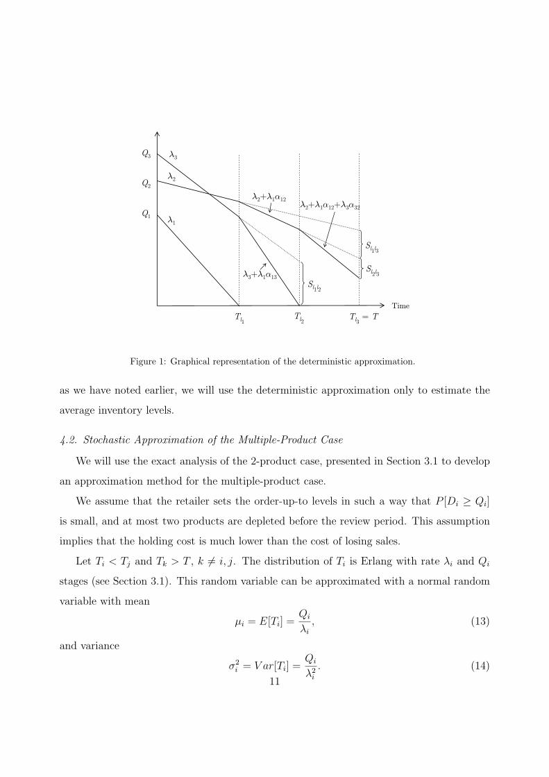
In Figure 1, we present a graphical representation of a system with 3 products, and
with l1 = 1 and l2 = 3. In the example presented in Figure 1, Product 2 is not depleted
within the review period, and completes the period with positive stock. The above outlined
approximation scheme can be generalized by defining ln and Tln , n = 1, ..., N as follows:
ln = arg mini;i 6=l1,...,ln−1
Qi −∑n−1j=1 (Tlj − Tlj−1
)(λi +∑j−1k=1 λlkαlki)
λi +∑n−1j=1 λljαlji
,
and
Tln = min{T,Qln −
∑n−1j=1 (Tlj − Tlj−1
)(λln +∑j−1k=1 λlkαlkln)
λln +∑n−1j=1 λljαlj ln
}.
Once the ln and Tln , n = 1, ..., N values are computed, the average inventory levels can
be computed in a straightforward manner by considering beginning and ending inventories
of each product in periods defined by the Tln , n = 1, ..., N values. As illustrated in Figure 1,
the substitutions between the products can be computed comparing the direct and effective
demand rates of each product in periods formed by the Tln , n = 1, ..., N values. However,
10
Q1
Q2
Q3
Tl1Tl3
= TTl2
Time
λ1
λ2
λ3
λ2+λ1α12
λ3+λ1α13
λ2+λ1α12+λ3α32
Sl1l2
Sl1l3
Sl2l3
Figure 1: Graphical representation of the deterministic approximation.
as we have noted earlier, we will use the deterministic approximation only to estimate the
average inventory levels.
4.2. Stochastic Approximation of the Multiple-Product Case
We will use the exact analysis of the 2-product case, presented in Section 3.1 to develop
an approximation method for the multiple-product case.
We assume that the retailer sets the order-up-to levels in such a way that P [Di ≥ Qi]
is small, and at most two products are depleted before the review period. This assumption
implies that the holding cost is much lower than the cost of losing sales.
Let Ti < Tj and Tk > T , k 6= i, j. The distribution of Ti is Erlang with rate λi and Qi
stages (see Section 3.1). This random variable can be approximated with a normal random
variable with mean
µi = E[Ti] =Qi
λi, (13)
and variance
σ2i = V ar[Ti] =
Qi
λ2i
. (14)
11
Note that this approximation follows the central limit theorem and quite accurate for large
values of Qi. Similarly, when Ti < Tj, assuming constant demand and substitution rates, Tj
can be approximated with a normal distribution with mean
µj = E[Tj] =Qj − (Qi/λi)λjλj + αijλi
+Qi
λi, (15)
and variance
σ2j = V ar[Tj] =
Qj − (Qi/λi)λj(λj + αijλi)2
+Qi
λi
1
λj. (16)
We assume that Ti and Tj are independent. We know from Section 3.1 that Ti and Tj
are not independent. However, when Ti < T < Tj, the effect of this approximation on
E[(T −Ti)+] will not be significant. Similarly, when Ti < Tj < T , the effect on E[(Tj−Ti)+]
will not be significant.
Let Γij be the length of the time Product i is substituted with Product j.
Γij =
T − Ti Ti < T < Tj
Tj − Ti Ti < Tj < T
0 T < min{Ti, Tj}
(17)
Under the above stated assumptions and following Equation (17),
E[Γij] ∼= E[(T − Ti)+, Ti < T < Tj] + E[(Tj − Ti)+, Ti < Tj < T ].
Furthermore, since it is assumed that Ti and Tj are independent,
E[Γij] ∼= E[(T − Ti)+]P [T < Tj] + E[(Tj − Ti)+|Ti < Tj < T ]P [Ti < T ]P [Tj < T ].
Note that with the normal approximation of Ti and Tj, we can determine E[(T − Ti)+],
E[(Tj − Ti)+] and P [Ti < T ] directly. Let η(z) be the expected number of units short of a
standard normal random variable:
η(z) =
∞∫z
1√2π
(x− z)e−12x2
dx = φ(z)− zΦ(z) (18)
where φ(z) and Φ(z) are the density function and cumulative distribution function of the
standard normal given as φ(z) = e−12z2 and Φ(z) =
∞∫zφ(z)dz. We can then write the
12
expected values as
E[(T − Ti)+] = T − µi + σiη(T − µiσi
), (19)
E[(T − Ti)+] = T − µi + σi
(φ(T − µiσi
)−(T − µiσi
)Φ(T − µiσi
)), (20)
and
E[(Ti − Tj)+|Ti < Tj < T ] = σji
(φ
(µjiσji
)− µjiσji
Φ
(µjiσji
)+ φ
(T + µjiσji
)+T + µjiσji
Φ
(T + µjiσji
))
−TΦ
(T + µjiσji
), (21)
where Tj − Ti is approximately normal with mean
µji = E[Tj − Ti] = E[Tj]− E[Ti], (22)
and variance
σ2ji = V ar[Tj − Ti] = V ar[Tj] + V ar[Ti], (23)
where the first term is determined in closed form following Equation (21) and the second term
is also given in closed form in Equation (20). E[(T−Tj)+] and E[(Tj−Ti)+|Ti < Tj < T ] can
be expressed in a similar fashion. The expected time Product i is substituted with Product
j Γij can be written as
Γij = E[(Tj − Ti)+|Ti < Tj < T ](
1− Φ(T − µiσi
))(1− Φ
(T − µjσj
))
+E[(T − Ti)+]Φ
(T − µjσj
). (24)
As a result, we can determine Sij i 6= j as
Sij = E[Γij]λiαij, (25)
and Sii as
Sii = E[min{Qi, λiT}]. (26)
Following the normal approximation, Sii can be evaluated as
Sii = λiT −√λiT
[φ
(Qi − λiT√
λiT
)−(Qi − λiT√
λiT
)(1− Φ
(Qi − λiT√
λiT
))](27)
13
Finally, if this approximation yields Sij values such that∑j Sij ≥ Qi, we normalize the
values such that
Sij = SijQi∑j Sij
.
5. Computational Study: Accuracy of the Approximation Approaches
In this section, we present a computational analysis of the approximation quality of the
approaches developed in Section 4. In the computational analysis, we consider a set of
randomly created 4-product problems. As noted in Karabati, Tan, and Ozturk [6], when
the observed number of substitutions is not statically significant, estimation of substitution
probabilities is a very challenging task. To deal with this issue, a certain number of products
with similar characteristics can be lumped together for analysis purposes. For example,
modeling the first three products with the largest market shares explicitly, and lumping
the other products with smaller market shares into a single product yields a model with 4
products. The performance of a model of this size can be evaluated quite accurately by using
the approximation method presented in this study and also can be optimized effectively.
The products’ order-up-to levels are set to satisfy a randomly selected fill rate without
taking the substitution effect into account. Three different service level ranges, [60%, 99%],
[70%, 99%], [80%, 99%], are used in problem generation, and the target service level of each
product is randomly selected using a uniform distribution between the lower and upper
limits of the ranges. The demand rates of the Product 1 and 2 (3 and 4) are generated
using a uniform distribution in the [15, 25] ([5, 15]) range. The customer choice model is
assumed to be Market-Share Based (see Smith and Agrawal [17], Netessine and Rudi [13],
and Kok and Fisher [8]) where the substitute product is chosen according to the substitution
probability matrix αij = θ λj∑l∈N\{i}
λl, i, j = 1, 2, . . . , N, and i 6= j. The review time is taken as
20 times units, and the substitution probability, θ, is taken as 60%. For each service level
range, 120 problems are randomly generated and simulated for 10 independent replications
with 50 review periods in each replication.
In Table 1, we report the deterministic approximation’s performance for products’ aver-
14
age inventory levels, and stochastic approximation’s performance for products’ total direct
sales, and total sales. The average and maximum approximation errors are reported, over
120 problems in each row of Table 1, relative to the average performance observed over 10
replications of the simulation model in each problem instance.
We note that, in order to capture the probabilistic nature of substitutions, all perfor-
mance measures, with the exception of inventory levels, are estimated with the probabilistic
approximation. The figures presented in Table 1 indicate that the inventory levels, prod-
ucts’ total direct and total sales can be closely estimated with approximation approaches
described earlier.
In Figure 2, we report the average performance of the probabilistic approach in estimat-
ing the number of substitutions between products. We first note that the performance of
the approximation approach is dependent on the rate of the realized substitutions: when
the number of substitutions per review period is low, the observations are not statistically
significant, and approximations are relatively poor. In light of this observation, we report
the approximation performance for 3 different minimum levels of substituted demand. For
example, when the minimum level is taken as 1%, and when the estimated number of sub-
stitutions from Product i to Product j, i.e., Sij, is less than λi×T ×0.01, substitutions from
Product i to Product j is considered to be statistically insignificant, and approximation
error with Sij is not included in the reported average approximation errors. In Figure 2, we
observe that the approximation quality increases when minimum level of statistical signifi-
cance and the variability in service levels increase. As we discuss in the next section, where
a model to find the optimal order-up-to levels under substitution is presented, we need bet-
ter substitution approximations in cases where the service level of a product is deliberately
set low to channel some of its demand to other products through substitutions. In these
instances, because the number of substitutions is high, the approximation quality of the
probabilistic approach will be high too.
15
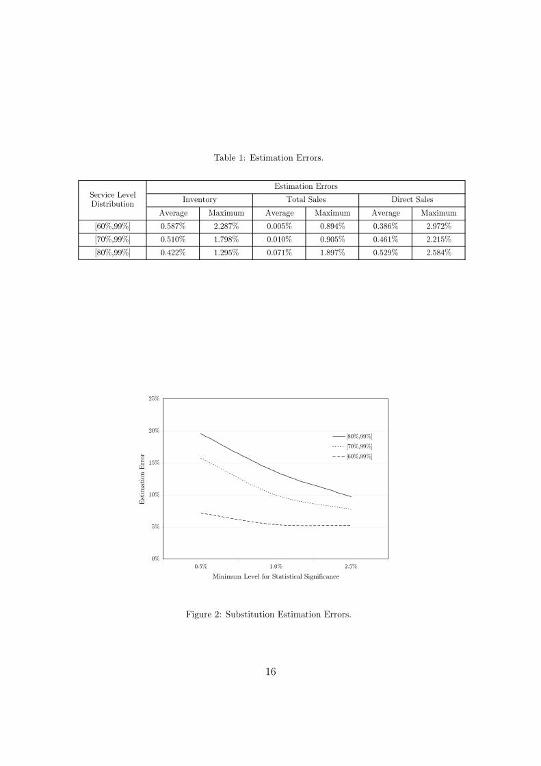
Table 1: Estimation Errors.
Average Maximum Average Maximum Average Maximum
[60%,99%] 0.587% 2.287% 0.005% 0.894% 0.386% 2.972%
[70%,99%] 0.510% 1.798% 0.010% 0.905% 0.461% 2.215%
[80%,99%] 0.422% 1.295% 0.071% 1.897% 0.529% 2.584%
Direct SalesService Level Distribution
Estimation Errors
Inventory Total Sales
0%
5%
10%
15%
20%
25%
0.5% 1.0% 2.5%
Minimum Level for Statistical Significance
Est
imat
ion E
rror
[80%,99%]
[70%,99%]
[60%,99%]
Figure 2: Substitution Estimation Errors.
16
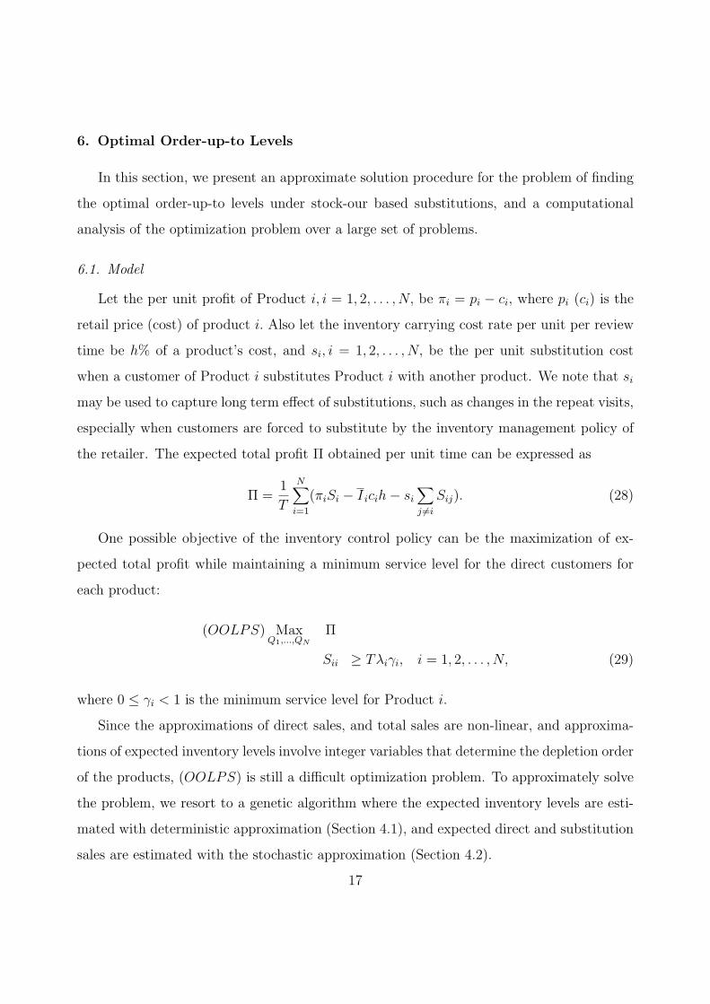
6. Optimal Order-up-to Levels
In this section, we present an approximate solution procedure for the problem of finding
the optimal order-up-to levels under stock-our based substitutions, and a computational
analysis of the optimization problem over a large set of problems.
6.1. Model
Let the per unit profit of Product i, i = 1, 2, . . . , N, be πi = pi − ci, where pi (ci) is the
retail price (cost) of product i. Also let the inventory carrying cost rate per unit per review
time be h% of a product’s cost, and si, i = 1, 2, . . . , N, be the per unit substitution cost
when a customer of Product i substitutes Product i with another product. We note that si
may be used to capture long term effect of substitutions, such as changes in the repeat visits,
especially when customers are forced to substitute by the inventory management policy of
the retailer. The expected total profit Π obtained per unit time can be expressed as
Π =1
T
N∑i=1
(πiSi − I icih− si∑j 6=i
Sij). (28)
One possible objective of the inventory control policy can be the maximization of ex-
pected total profit while maintaining a minimum service level for the direct customers for
each product:
(OOLPS) MaxQ1,...,QN
Π
Sii ≥ Tλiγi, i = 1, 2, . . . , N, (29)
where 0 ≤ γi < 1 is the minimum service level for Product i.
Since the approximations of direct sales, and total sales are non-linear, and approxima-
tions of expected inventory levels involve integer variables that determine the depletion order
of the products, (OOLPS) is still a difficult optimization problem. To approximately solve
the problem, we resort to a genetic algorithm where the expected inventory levels are esti-
mated with deterministic approximation (Section 4.1), and expected direct and substitution
sales are estimated with the stochastic approximation (Section 4.2).
17
6.2. Computational Analysis
In this section, we report our computational experience with the optimization problem
outlined in the previous section. We first discuss two problem instances, then analyze the
results over a larger set of problems.
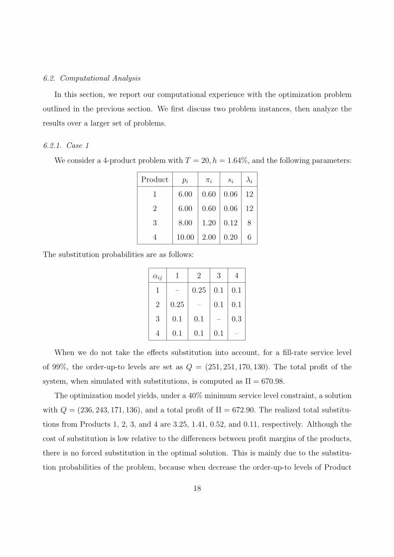
6.2.1. Case 1
We consider a 4-product problem with T = 20, h = 1.64%, and the following parameters:
Product pi πi si λi
1 6.00 0.60 0.06 12
2 6.00 0.60 0.06 12
3 8.00 1.20 0.12 8
4 10.00 2.00 0.20 6
The substitution probabilities are as follows:
αij 1 2 3 4
1 – 0.25 0.1 0.1
2 0.25 – 0.1 0.1
3 0.1 0.1 – 0.3
4 0.1 0.1 0.1 –
When we do not take the effects substitution into account, for a fill-rate service level
of 99%, the order-up-to levels are set as Q = (251, 251, 170, 130). The total profit of the
system, when simulated with substitutions, is computed as Π = 670.98.
The optimization model yields, under a 40% minimum service level constraint, a solution
with Q = (236, 243, 171, 136), and a total profit of Π = 672.90. The realized total substitu-
tions from Products 1, 2, 3, and 4 are 3.25, 1.41, 0.52, and 0.11, respectively. Although the
cost of substitution is low relative to the differences between profit margins of the products,
there is no forced substitution in the optimal solution. This is mainly due to the substitu-
tion probabilities of the problem, because when decrease the order-up-to levels of Product
18
1 and/or 2 to increase substitution from these products to more profitable products, i.e.,
Products 3 and 4, a substantial portion of their demand is lost.
When we increase α1,3 and α2,3 to 0.3, the optimal solution becomesQ = (97, 276, 207, 139),
with a total profit of Π = 680.00. Because of its low order-up-to level, the direct sales of
Product 1 realizes as 40%, the minimum level required by the direct service level constraint.
The realized total substitutions from Products 1, 2, 3, and 4 are now 89.35, 1.55, 0.82, and
0.29, respectively. We note that, in the optimal solution, forced substitution is observed in
only one of the less profitable products. The substitution probabilities between Products 1
and 2 (α1,2 = α2,1 = 0.25) are significant, and lowering the order-up-to levels of Products 1
and 2 simultaneously results in lost sales when customers of Products 1 and 2 attempt to
substitute their preferred product with another one.
When we increase α1,3 and α2,3 to 0.5, a major portion of customers of both Product 1 and
Product 2 are forced to substitute, because, in the optimal solution, the order-up-to levels
are set as Q = (98, 99, 302, 149). The total profit of the system is now Π = 715.60. Although
we lost 25% of demands of Products 1 and 2, we recover lost sales with the increased profits
when 28% of customers of Products 1 and 2 substitute with Product 3.
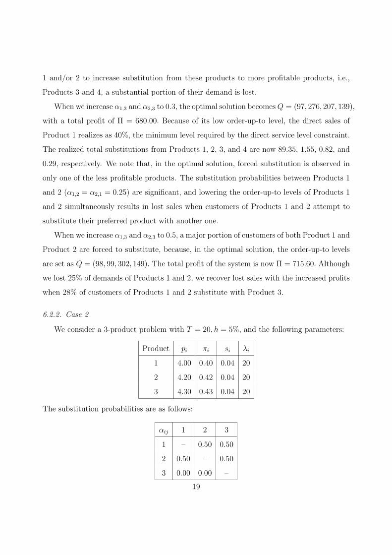
6.2.2. Case 2
We consider a 3-product problem with T = 20, h = 5%, and the following parameters:
Product pi πi si λi
1 4.00 0.40 0.04 20
2 4.20 0.42 0.04 20
3 4.30 0.43 0.04 20
The substitution probabilities are as follows:
αij 1 2 3
1 – 0.50 0.50
2 0.50 – 0.50
3 0.00 0.00 –
19
In this example, although substitution costs are higher than the profit margin differences,
we obtain an optimal solution with Q = (352, 422, 423), and Π = 367.77. Approximately
10% of Product 1’s demand is substituted with Products 2 and 3, in equal proportions.
When we do not take the effects substitution into account, for a fill-rate service level of
99%, the order-up-to levels are set as Q = (410, 410, 410), and total profit of the system,
when simulated with substitutions, is computed as Π = 366.46. Because the holding cost
rate is high in this particular problem, the first solution creates a partial “pooling effect”
for demands of Products 1 and 2, and 1 and 3 by channeling 10% of Product 1’s demand
through substitutions. This in turn decreases the inventory costs, and results in a slightly
better total profit. We note that the optimal solution of Q = (352, 422, 423) starts the
period with a total of 1198 units of inventory, and the 99% fill-rate solution’s initial total
inventory is equal to 1230 units.
6.2.3. Randomly Generated Problems
In this section we consider a larger set of randomly created problems to study the impact
of substitutions on system’s profit performance.
We consider 4-product problems with identical costs, four demand scenarios ((10,10,10,10),
(15,15,5,5), (12,12,8,8), and (20,10,5,5)), four levels of substitution costs (0%, 5%, 10%, and
25% of products’ profit margins), and nine market share dependent profit margin scenarios
where πi =(A−B λi∑
jλj
)with (A,B) ∈ {(0.2, 0.3), (0.2, 0.2), (0.2, 0.1), (0.1, 0.15), (0.1, 0.1),
(0.1, 0.05), (0.05, 0.075), (0.05, 0.05), (0.05, 0.025)}. We note that, according to above expres-
sion, profit margins are negatively correlated with market shares.
The problem generation scheme results in 144 test problems with profit margins that are
negatively correlated with market shares, and identical product costs. The customer choice
model is again assumed to be Market-Share Based (see Section 5).
For comparison purposes, we create a benchmark solution for every problem instance.
We first solve a given problem instance optimally, as outlined in Section 6.1, and then
compute the value of the initial inventory by multiplying the optimal order-up-to levels
by the corresponding product costs. We then find the fill-rate service level that would
20
94%
95%
96%
97%
98%
99%
100%
60% 70% 80% 90% 100%
Substitution Probability
Ben
chm
ark S
ervic
e Lev
el
0%
1%
2%
3%
4%
5%
6%
Pro
fit
Impro
vem
ent
Benchmark Service Level
Profit Improvement
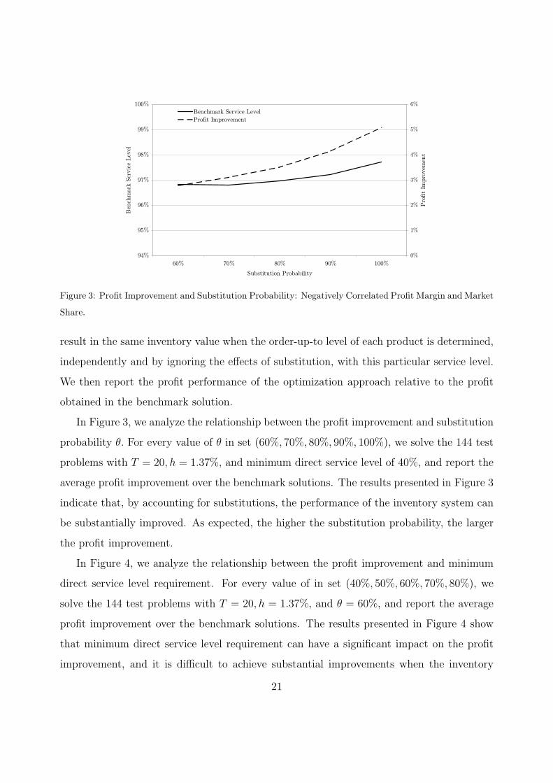
Figure 3: Profit Improvement and Substitution Probability: Negatively Correlated Profit Margin and Market
Share.
result in the same inventory value when the order-up-to level of each product is determined,
independently and by ignoring the effects of substitution, with this particular service level.
We then report the profit performance of the optimization approach relative to the profit
obtained in the benchmark solution.
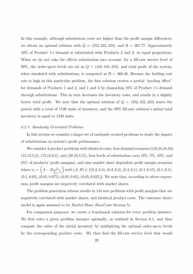
In Figure 3, we analyze the relationship between the profit improvement and substitution
probability θ. For every value of θ in set (60%, 70%, 80%, 90%, 100%), we solve the 144 test
problems with T = 20, h = 1.37%, and minimum direct service level of 40%, and report the
average profit improvement over the benchmark solutions. The results presented in Figure 3
indicate that, by accounting for substitutions, the performance of the inventory system can
be substantially improved. As expected, the higher the substitution probability, the larger
the profit improvement.
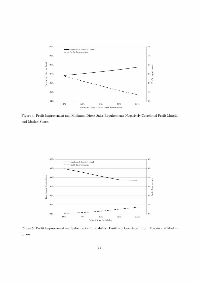
In Figure 4, we analyze the relationship between the profit improvement and minimum
direct service level requirement. For every value of in set (40%, 50%, 60%, 70%, 80%), we
solve the 144 test problems with T = 20, h = 1.37%, and θ = 60%, and report the average
profit improvement over the benchmark solutions. The results presented in Figure 4 show
that minimum direct service level requirement can have a significant impact on the profit
improvement, and it is difficult to achieve substantial improvements when the inventory
21
94%
95%
96%
97%
98%
99%
100%
40% 50% 60% 70% 80%
Minimum Direct Service Level Requirement
Ben
chm
ark S
ervic
e Lev
el
0%
1%
2%
3%
4%
5%
6%
Pro
fit
Impro
vem
ent
Benchmark Service Level
Profit Improvement
Figure 4: Profit Improvement and Minimum Direct Sales Requirement: Negatively Correlated Profit Margin
and Market Share.
94%
95%
96%
97%
98%
99%
100%
60% 70% 80% 90% 100%
Substitution Probability
Ben
chm
ark S
ervic
e Lev
el
0%
1%
2%
3%
4%
5%
6%
Pro
fit
Impro
vem
ent
Benchmark Service Level
Profit Improvement
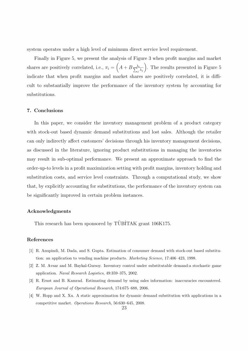
Figure 5: Profit Improvement and Substitution Probability: Positively Correlated Profit Margin and Market
Share.
22
system operates under a high level of minimum direct service level requirement.
Finally in Figure 5, we present the analysis of Figure 3 when profit margins and market
shares are positively correlated, i.e., πi =(A+B λi∑
jλj
). The results presented in Figure 5
indicate that when profit margins and market shares are positively correlated, it is diffi-
cult to substantially improve the performance of the inventory system by accounting for
substitutions.
7. Conclusions
In this paper, we consider the inventory management problem of a product category
with stock-out based dynamic demand substitutions and lost sales. Although the retailer
can only indirectly affect customers’ decisions through his inventory management decisions,
as discussed in the literature, ignoring product substitutions in managing the inventories
may result in sub-optimal performance. We present an approximate approach to find the
order-up-to levels in a profit maximization setting with profit margins, inventory holding and
substitution costs, and service level constraints. Through a computational study, we show
that, by explicitly accounting for substitutions, the performance of the inventory system can
be significantly improved in certain problem instances.
Acknowledgments
This research has been sponsored by TUBITAK grant 106K175.
References
[1] R. Anupindi, M. Dada, and S. Gupta. Estimation of consumer demand with stock-out based substitu-
tion: an application to vending machine products. Marketing Science, 17:406–423, 1998.
[2] Z. M. Avsar and M. Baykal-Gursoy. Inventory control under substitutable demand:a stochastic game
application. Naval Research Logistics, 49:359–375, 2002.
[3] R. Ernst and B. Kamrad. Estimating demand by using sales information: inaccuracies encountered.
European Journal of Operational Research, 174:675–688, 2006.
[4] W. Hopp and X. Xu. A static approximation for dynamic demand substitution with applications in a
competitive market. Operations Research, 56:630–645, 2008.23
[5] V. N. Hsu, C. Li, and W. Xiao. Dynamic lot size problems with one-way product substitution. IIE
Transactions, 37:201–215, 2005.
[6] S. Karabatı, B. Tan, and C. Ozturk. A method for estimating stock-out based substitution rates by
using point-of-sale data. IIE Transactions, 41:408–420, 2009.
[7] A. Kok, M. Fisher, and R. Vaidyanathan. Assortment planning: Review of literature and industry
practice. In N. Agrawal and S. A. Smith, editors, Retail Supply Chain Management: Quantitative
Models and Empirical Studies, pages 99–154. Springer-Verlag New York, 2008.
[8] G. Kok and M. Fisher. Demand estimation and assortment optimization under substitution: Method-
ology and application. Operations Research, 55(6):1001–1021, 2007.
[9] S. Mahajan and G. van Ryzin. Retail inventories and consumer choice. In R. T. Sridhar, M. J.
Magazine, and R. Ganeshan, editors, Quantitative Models for Supply Chain Management, pages 491–
554. Springer-Verlag New York, 1998.
[10] S. Mahajan and G. van Ryzin. Stocking retail assortments under dynamic consumer substitution.
Operations Research, 49(3):334–351, 2001.
[11] A. McGillivray and E. Silver. Some concepts for inventory control under substitutable demands. IN-
FOR, 16(1):47–63, 1978.
[12] M. Nagarajan and S. Rajagopalan. Inventory models for substitutable products: Optimal policies and
heuristics. Management Science, 54(8):453–1466, 2008.
[13] S. Netessine and N. Rudi. Centralized and competitive inventory models with demand substitution.
Operations Research, 51(2):329–335, 2003.
[14] M. Parlar. Optimal ordering policies for a perishable and substitutable product: A markov decision
model. INFOR, 23:182–195, 1985.
[15] K. Rajaram and C. Tang. The impact of product substitution on retail merchandising. European
Journal of Operational Research, 135:582–601, 2001.
[16] U. S. Rao, J. M. Swaminathan, and J. Zhang. Multi-product inventory planning with downward
substitution, stochastic demand and setup costs. IIE Transactions, 36:59–71, 2004.
[17] S. Smith and N. Agrawal. Management of multi-item retail inventory systems with demand substitution.
Operations Research, 48(1):50–64, 2000.
[18] E. Yucel, F. Karaesmen, F. S. Salman, and M. Turkay. Optimizing product assortment under customer-
driven demand substitution. European Journal of Operational Research, 2009. forthcoming.
24