Results of Validation Tests Applied to Seven ENERGY STAR Building Models

John H. Scofield, Oberlin College, Oberlin, OH Gabriel Richman, Oberlin College, Oberlin, OH

ABSTRACT  

In 1998 the EPA introduced its ENERGY STAR building benchmarking score for Office buildings as part of a broad set of initiatives to promote efficient use of energy. Since then the EPA has developed benchmarking scores for a total of 12 conventional building types. The central feature of the ENERGY STAR methodology is a multivariate regression performed on a nationally representative sample of buildings of a particular type. This regression is used to adjust the energy used by a building for external factors identified by the EPA that drive building energy use. The EPA has never published evidence that these regressions are valid for buildings outside the sampled datasets. So called validation is a crucial step for making use of any such regression results.

Here we report results for validation tests performed on seven of the ENERGY STAR building models that are based on CBECS data. For six of these, external validation was accomplished by constructing equivalent model datasets from a different vintage of CBECS from that used by the EPA. For the seventh model (Supermarket/Grocery Store) an internal validation method was employed. One model (Office) passes validation indicting its weighted regression is largely reproducible. In contrast, four models (Worship Facility, Supermarket/Grocery, Warehouse, and K-12 Schools) fail validation suggesting the opposite and casting doubt on the utility of ENERGY STAR scores for these buildings. Validation tests for the other two models (Hotel/Motel and Retail Stores) yield intermediate results indicating some consistency yet with large uncertainties in their ENERGY STAR scores.

1. Introduction

Building energy benchmarking is a process in which the energy used by a particular building is compared with the energy used by other, similar buildings. Historically, benchmarking provides a simple method for a building portfolio manager to identify the poorly-performing buildings which are most likely to benefit from energy-efficiency upgrades. More recently energy benchmarking scores have been cited for building portfolios as evidence for energy savings (EPA 2012, USGBC 2012). As larger buildings use more energy than smaller buildings the preferred metric for building energy use is the annual energy use intensity (e) or EUI, calculated by dividing a building’s annual energy use (E) by its gross floor area (A), namely e = E/A. A building’s annual site energy is readily determined by totaling monthly energy purchases after first converting fuel quantities to a common energy unit, typically British thermal units (Btu) or mega Joules (MJ).

Building site energy, however, fails to account for the off-site energy losses incurred in producing the energy and delivering it to the building, particularly important for electric energy. The U.S. Environmental Protection Agency (EPA) defines building source energy to account for both on- and off-site energy consumption associated with a building. Source energy is calculated by totaling annual energy purchases after multiplying each by a fuel-dependent, national-average site-to-source energy conversion factor (EPA 2011). In this paper all references to building energy (or EUI) refer to source energy (or source EUI).

Energy benchmarking is done by building type. Hospitals, for instance, use more energy than warehouses so it makes no sense to compare the two. Once a building type has been chosen the next

  

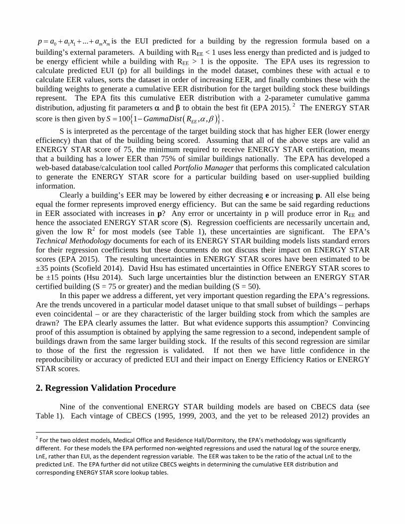
step in developing a benchmarking scale is to obtain energy performance data for a statistically significant number of buildings of this type that adequately characterize the target building stock. The EPA has developed energy benchmarking scores for 12 conventional types of buildings listed in Table 1. For each building type the target stock is a subset of the national building stock that meet certain specific criteria listed in Technical Methodology documents published for each building type (EPA 2015). Most of the EPA building models rely on data obtained from one of the Energy Information Administration’s Commercial Building Energy Consumption Surveys (CBECS).1 The three most recent surveys were conducted for 2003, 1999, and 1995. For three building types the EPA has relied instead on data obtained from industry surveys conducted by or in collaboration with a relevant trade organization (see Table 1). The EPA revises its building models over time. Table 1 lists the latest revision date, the source of model data, the number of samples (n) in the model dataset and the estimated number of buildings in the target building stock they represent (N). Also listed are characteristics of the EPA model regressions (discussed below).

Table 1. Table summarizing models for 12 conventional building types. n is the number of samples in the regression dataset, N is the number of U.S. buildings they represent, and R2 is the goodness of fit for the model regression using m independent variables.

There are various ways one might compare the EUI of a particular building to the distribution of EUI obtained for the target comparison building stock. The drawback with such direct comparisons is that annual energy use and EUI are affected by external factors that have nothing to do with energy efficiency – factors such as climate, weekly hours of operation, and numbers of employees. The EPA’s ENERGY STAR benchmarking system attempts to identify and adjust for such external factors. For a particular building type the EPA has searched through the model data to identify as many as m (an integer ranging from 1-11 depending on the building type) external factors 1 2, ,..., mx x x that correlate

with EUI (e). This process is mostly driven by statistical significance and data availability rather than any underlying engineering model. The EUI data in the model dataset are fit with a weighted, multivariate linear regression on these m-independent variables obtaining regression coefficients

0 1, ,..., ma a a . The R2 goodness of fit for these regressions and the number of fit parameters (m) are

listed in Table 1. The EPA defines the Energy Efficiency Ratio (EER) EER e p , where

                                                            1 CBECS uses a stratified random sampling technique in which the j‐th observation in the survey is associated with a weight (wj) that indicates the number of buildings in the U.S. commercial building stock represented by this sample. 

  

0 1 1 ... m mp a a x a x is the EUI predicted for a building by the regression formula based on a

building’s external parameters. A building with REE < 1 uses less energy than predicted and is judged to be energy efficient while a building with REE > 1 is the opposite. The EPA uses its regression to calculate predicted EUI (p) for all buildings in the model dataset, combines these with actual e to calculate EER values, sorts the dataset in order of increasing EER, and finally combines these with the building weights to generate a cumulative EER distribution for the target building stock these buildings represent. The EPA fits this cumulative EER distribution with a 2-parameter cumulative gamma distribution, adjusting fit parameters and to obtain the best fit (EPA 2015). 2 The ENERGY STAR score is then given by 100 1 , ,EES GammaDist R .

S is interpreted as the percentage of the target building stock that has higher EER (lower energy efficiency) than that of the building being scored. Assuming that all of the above steps are valid an ENERGY STAR score of 75, the minimum required to receive ENERGY STAR certification, means that a building has a lower EER than 75% of similar buildings nationally. The EPA has developed a web-based database/calculation tool called Portfolio Manager that performs this complicated calculation to generate the ENERGY STAR score for a particular building based on user-supplied building information.

Clearly a building’s EER may be lowered by either decreasing e or increasing p. All else being equal the former represents improved energy efficiency. But can the same be said regarding reductions in EER associated with increases in p? Any error or uncertainty in p will produce error in REE and hence the associated ENERGY STAR score (S). Regression coefficients are necessarily uncertain and, given the low R2 for most models (see Table 1), these uncertainties are significant. The EPA’s Technical Methodology documents for each of its ENERGY STAR building models lists standard errors for their regression coefficients but these documents do not discuss their impact on ENERGY STAR scores (EPA 2015). The resulting uncertainties in ENERGY STAR scores have been estimated to be ±35 points (Scofield 2014). David Hsu has estimated uncertainties in Office ENERGY STAR scores to be ±15 points (Hsu 2014). Such large uncertainties blur the distinction between an ENERGY STAR certified building (S = 75 or greater) and the median building (S = 50).

In this paper we address a different, yet very important question regarding the EPA’s regressions. Are the trends uncovered in a particular model dataset unique to that small subset of buildings – perhaps even coincidental – or are they characteristic of the larger building stock from which the samples are drawn? The EPA clearly assumes the latter. But what evidence supports this assumption? Convincing proof of this assumption is obtained by applying the same regression to a second, independent sample of buildings drawn from the same larger building stock. If the results of this second regression are similar to those of the first the regression is validated. If not then we have little confidence in the reproducibility or accuracy of predicted EUI and their impact on Energy Efficiency Ratios or ENERGY STAR scores.

2. Regression Validation Procedure

Nine of the conventional ENERGY STAR building models are based on CBECS data (see Table 1). Each vintage of CBECS (1995, 1999, 2003, and the yet to be released 2012) provides an

                                                            2 For the two oldest models, Medical Office and Residence Hall/Dormitory, the EPA’s methodology was significantly different.  For these models the EPA performed non‐weighted regressions and used the natural log of the source energy, LnE, rather than EUI, as the dependent regression variable.  The EER was taken to be the ratio of the actual LnE to the predicted LnE.  The EPA further did not utilize CBECS weights in determining the cumulative EER distribution and corresponding ENERGY STAR score lookup tables. 

  

independent snapshot of the U.S. commercial building stock. CBECS data since 1992 show that the commercial building stock has experienced an average growth rate of 1.7% per year (in gross square feet) with no significant change in gross site EUI. Thus it would appear that CBECS data from a different vintage from the one used by the EPA would provide independent data for externally validating an ENERGY STAR model regression. The Medical Office and Residence Hall/Dormitory models are based on 1999 CBECS. 2003 CBECS data, then, offer the opportunity to externally validate these models. External validation of these models is discussed elsewhere (Scofield 2014).

Six building models are based on 2003 CBECS data. Older, 1999 CBECS data provide opportunities to externally validate these models. The validation process is as follows. First we follow the EPA’s methodology to extract their model data (dataset A) from the 2003 CBECS dataset, calculate source EUI, and replicate the EPA’s weighted regression. Next, an independent model dataset (dataset B) is extracted from CBECS 1999 by applying the same data filters used by the EPA for the original CBECS 2003 model dataset. Source EUI are calculated for each building in this new dataset using the same site-to-source conversion factors used for the EPA model dataset. The EPA’s weighted regression is then performed on the new dataset. The results of the new regression (statistical significance and values for regression coefficients) are compared with the EPA’s results. The crucial test is to compare the predictions of these two regressions. Regression coefficients from the EPA’s analysis (A) and from the new dataset (B) are used to calculate two different predicted EUI values (pA and pB) for each building in one or both datasets. A graph of pB vs pA is used to assess the agreement in the two predictions. A diagonal line (pB = pA) shows excellent agreement while random scatter shows little agreement. The overall agreement is quantified by calculating the coefficient of determination, R2.3 3. Validation Results

External validation of the Medical Office and Residence Hall/Dormitory models has been discussed elsewhere (Scofield 2014). Both models failed these tests, suggesting that the regression results were not reproducible. In both cases the underlying problem is that the model datasets are simply too small to characterize their respective building stocks with sufficient accuracy to be of use for such analysis.

Below we describe the validation tests and their results for the remaining seven ENERGY STAR building models. For four of these difficulties arose in applying the EPA’s filters to 1999 CBECS data due to slight differences in the 1999 and 2003 CBECS surveys. For each of these models we were able to find a work-around that allowed for an “apples-to-apples” comparison. The details are discussed below. We begin by discussing results for Worship Facilities and Hotels/Motels which were free of these problems. 

3.1 Worship Facilities and Hotel/Motel

First consider the Worship Facility model (EPA 2015/Worship). Our replication of the EPA’s weighted regression (A) yielded a total R2 of 39%. Dataset B contained nB = 214 records corresponding to an estimated NB = 250,000 buildings in the 1999 building stock. Regression B on this dataset yielded a total R2 = 18%. The t-values and regression coefficients for the two regressions (A and B) showed marked differences.

                                                            3 Technically, the regression weights should be used to calculate weighted R2 values.  We, instead, provide un‐weighted R2 values as they correspond to the actual pB vs pA graphs (hard to plot a weighted graph).  We have also calculated the weighted R2 values and verified them to be qualitatively similar to the un‐weighted values presented.  

  

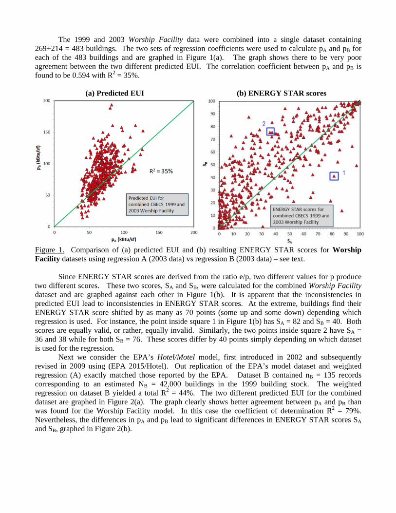
The 1999 and 2003 Worship Facility data were combined into a single dataset containing 269+214 = 483 buildings. The two sets of regression coefficients were used to calculate pA and pB for each of the 483 buildings and are graphed in Figure 1(a). The graph shows there to be very poor agreement between the two different predicted EUI. The correlation coefficient between pA and pB is found to be 0.594 with R2 = 35%.

(a) Predicted EUI (b) ENERGY STAR scores

Figure 1. Comparison of (a) predicted EUI and (b) resulting ENERGY STAR scores for Worship Facility datasets using regression A (2003 data) vs regression B (2003 data) – see text.

Since ENERGY STAR scores are derived from the ratio e/p, two different values for p produce two different scores. These two scores, SA and SB, were calculated for the combined Worship Facility dataset and are graphed against each other in Figure 1(b). It is apparent that the inconsistencies in predicted EUI lead to inconsistencies in ENERGY STAR scores. At the extreme, buildings find their ENERGY STAR score shifted by as many as 70 points (some up and some down) depending which regression is used. For instance, the point inside square 1 in Figure 1(b) has SA = 82 and SB = 40. Both scores are equally valid, or rather, equally invalid. Similarly, the two points inside square 2 have SA = 36 and 38 while for both SB = 76. These scores differ by 40 points simply depending on which dataset is used for the regression.

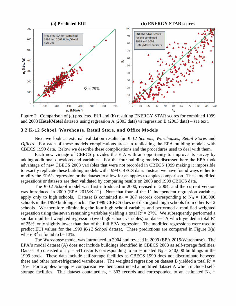
Next we consider the EPA’s Hotel/Motel model, first introduced in 2002 and subsequently revised in 2009 using (EPA 2015/Hotel). Out replication of the EPA’s model dataset and weighted regression (A) exactly matched those reported by the EPA. Dataset B contained nB = 135 records corresponding to an estimated NB = 42,000 buildings in the 1999 building stock. The weighted regression on dataset B yielded a total R2 = 44%. The two different predicted EUI for the combined dataset are graphed in Figure 2(a). The graph clearly shows better agreement between pA and pB than was found for the Worship Facility model. In this case the coefficient of determination R2 = 79%. Nevertheless, the differences in pA and pB lead to significant differences in ENERGY STAR scores SA and SB, graphed in Figure 2(b).

  

(a) Predicted EUI (b) ENERGY STAR scores

Figure 2. Comparison of (a) predicted EUI and (b) resulting ENERGY STAR scores for combined 1999 and 2003 Hotel/Motel datasets using regression A (2003 data) vs regression B (2003 data) – see text.

3.2 K-12 School, Warehouse, Retail Store, and Office Models

Next we look at external validation results for K-12 Schools, Warehouses, Retail Stores and Offices. For each of these models complications arose in replicating the EPA building models with CBECS 1999 data. Below we describe these complications and the procedures used to deal with them.

Each new vintage of CBECS provides the EIA with an opportunity to improve its survey by adding additional questions and variables. For the four building models discussed here the EPA took advantage of new CBECS 2003 variables that were not recorded in CBECS 1999 making it impossible to exactly replicate these building models with 1999 CBECS data. Instead we have found ways either to modify the EPA’s regression or the dataset to allow for an apples-to-apples comparison. These modified regressions or datasets are then validated by comparing results on 2003 and 1999 CBECS data.

The K-12 School model was first introduced in 2000, revised in 2004, and the current version was introduced in 2009 (EPA 2015/K-12). Note that four of the 11 independent regression variables apply only to high schools. Dataset B contained nB = 387 records corresponding to NB = 130,000 schools in the 1999 building stock. The 1999 CBECS does not distinguish high schools from other K-12 schools. We therefore eliminating the four high school variables and performed a modified weighted regression using the seven remaining variables yielding a total R2 = 27%. We subsequently performed a similar modified weighted regression (w/o high school variables) on dataset A which yielded a total R2 of 25%, only slightly lower than that of the full EPA regression. The modified regressions were used to predict EUI values for the 1999 K-12 School dataset. These predictions are compared in Figure 3(a) where R2 is found to be 13%.

The Warehouse model was introduced in 2004 and revised in 2009 (EPA 2015/Warehouse). The EPA’s model dataset (A) does not include buildings identified in CBECS 2003 as self-storage facilities. Dataset B consisted of nB = 541 records corresponding to an estimated NB = 240,000 buildings in the 1999 stock. These data include self-storage facilities as CBECS 1999 does not discriminate between these and other non-refrigerated warehouses. The weighted regression on dataset B yielded a total R2 = 19%. For a apples-to-apples comparison we then constructed a modified dataset A which included self-storage facilities. This dataset contained nA = 303 records and corresponded to an estimated NA =

  

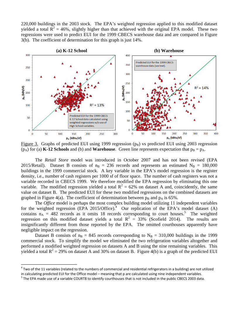
220,000 buildings in the 2003 stock. The EPA’s weighted regression applied to this modified dataset yielded a total R2 = 46%, slightly higher than that achieved with the original EPA model. These two regressions were used to predict EUI for the 1999 CBECS warehouse data and are compared in Figure 3(b). The coefficient of determination for this graph is just 14%.

  (a) K-12 School (b) Warehouse

Figure 3. Graphs of predicted EUI using 1999 regression (pB) vs predicted EUI using 2003 regression (pA) for (a) K-12 Schools and (b) and Warehouse. Green line represents expectation that pB = pA.

The Retail Store model was introduced in October 2007 and has not been revised (EPA 2015/Retail). Dataset B consists of nB = 236 records and represents an estimated NB = 180,000 buildings in the 1999 commercial stock. A key variable in the EPA’s model regression is the register density, i.e., number of cash registers per 1000 sf of floor space. The number of cash registers was not a variable recorded in CBECS 1999. We therefore modified the EPA regression by eliminating this one variable. The modified regression yielded a total R2 = 62% on dataset A and, coincidently, the same value on dataset B. The predicted EUI for these two modified regressions on the combined datasets are graphed in Figure 4(a). The coefficient of determination between pB and pA is 65%.

The Office model is perhaps the most complex building model utilizing 11 independent variables for the weighted regression (EPA 2015/Office).4 Our replication of the EPA’s model dataset (A) contains nA = 482 records as it omits 18 records corresponding to court houses.5 The weighted regression on this modified dataset yields a total R2 = 33% (Scofield 2014). The results are insignificantly different from those reported by the EPA. The omitted courthouses apparently have negligible impact on the regression.

Dataset B consists of nB = 845 records corresponding to NB = 310,000 buildings in the 1999 commercial stock. To simplify the model we eliminated the two refrigeration variables altogether and performed a modified weighted regression on datasets A and B using the nine remaining variables. This yielded a total R2 = 29% on dataset A and 30% on dataset B. Figure 4(b) is a graph of the predicted EUI

                                                            4 Two of the 11 variables (related to the numbers of commercial and residential refrigerators in a building) are not utilized in calculating predicted EUI for the Office model – meaning that p are calculated using nine independent variables. 5 The EPA made use of a variable COURT8 to identify courthouses that is not included in the public CBECS 2003 data. 

  

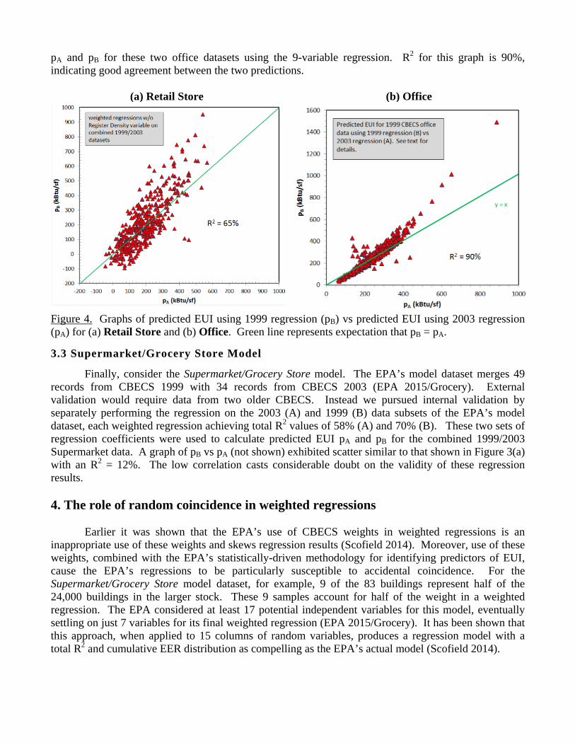
pA and pB for these two office datasets using the 9-variable regression. R2 for this graph is 90%, indicating good agreement between the two predictions.

(a) Retail Store (b) Office

Figure 4. Graphs of predicted EUI using 1999 regression (pB) vs predicted EUI using 2003 regression (pA) for (a) Retail Store and (b) Office. Green line represents expectation that pB = pA.

3.3 Supermarket/Grocery Store Model

Finally, consider the Supermarket/Grocery Store model. The EPA’s model dataset merges 49 records from CBECS 1999 with 34 records from CBECS 2003 (EPA 2015/Grocery). External validation would require data from two older CBECS. Instead we pursued internal validation by separately performing the regression on the 2003 (A) and 1999 (B) data subsets of the EPA’s model dataset, each weighted regression achieving total R2 values of 58% (A) and 70% (B). These two sets of regression coefficients were used to calculate predicted EUI pA and pB for the combined 1999/2003 Supermarket data. A graph of pB vs pA (not shown) exhibited scatter similar to that shown in Figure 3(a) with an R2 = 12%. The low correlation casts considerable doubt on the validity of these regression results.

4. The role of random coincidence in weighted regressions

Earlier it was shown that the EPA’s use of CBECS weights in weighted regressions is an inappropriate use of these weights and skews regression results (Scofield 2014). Moreover, use of these weights, combined with the EPA’s statistically-driven methodology for identifying predictors of EUI, cause the EPA’s regressions to be particularly susceptible to accidental coincidence. For the Supermarket/Grocery Store model dataset, for example, 9 of the 83 buildings represent half of the 24,000 buildings in the larger stock. These 9 samples account for half of the weight in a weighted regression. The EPA considered at least 17 potential independent variables for this model, eventually settling on just 7 variables for its final weighted regression (EPA 2015/Grocery). It has been shown that this approach, when applied to 15 columns of random variables, produces a regression model with a total R2 and cumulative EER distribution as compelling as the EPA’s actual model (Scofield 2014).

  

Weighted regressions skew the results of all of the seven models considered in this paper. The question arises as to how these weights affect the validation tests discussed above. For each model would non-weighted regressions on datasets A and B produce more consistent results? To address this we have reproduced the above regressions – but without weights – for several of the models and found that of graphs of pB vs pA show much more correlation than for the weighted regressions. Of course the statistical significances of the variables in predicting EUI and the total R2 for these regressions are quite different from those found for weighted regressions. Still, preliminary results suggest that non-weighted regressions yield far more consistent pA and pB. 5. Discussion

The strong correlation exhibited in Figure 4(b) confirms the consistency of the EPA’s weighted regression for the Office model. Regressions performed on two independent representative subsets of the office building stock produce similar results giving us some confidence in the EUI predicted by the EPA model. This model has other problems associated with inappropriate use of weights in the regression (Scofield 2014) but here it passes the external validation test for consistency.

In contrast the low correlation found in Figures 1, 3(a), 3(b), and 4(a) suggest that the weighted regressions for the Worship Facility, Warehouse, K-12 School, and Supermarket/Grocery Store ENERGY STAR models are not reproducible – and variations in ENERGY STAR scores associated with variations in predicted EUI for these models are not meaningful.

For the last two models, Hotel/Motel and Retail Stores, Figures 2(a) and 4(a) show moderate correlation, suggesting these weighted regressions contain some reproducible elements but that their predicted EUI still have significant uncertainty which lead to substantial variation in ENERGY STAR scores, as demonstrated for the Hotel/Motel model in Figure 2(b).

The problem with using ENERGY STAR scores based on invalid regressions for evaluating building performance is illustrated in Figure 1(b) for Worship Facilities. Earlier I discussed several buildings (squares 1 and 2 in the figure) whose scores differ by 40 points depending on which dataset are used for the regression. These results are not unusual. ENERGY STAR scores for buildings in the middle two quartiles tend to be sensitive to p. 84 buildings in Figure 1(b) have SA in the second quartile

26 50AS ; 46 of these – more than half – have scores SB in the third quartile 51 75BS . A

building portfolio manager would be ill-advised to use these ENERGY STAR scores to decide which buildings should receive energy efficiency upgrades. Similarly, a municipality would be ill advised to rely on such ENERGY STAR scores to judge progress in improving the energy performance of its buildings over time. And, given the fact that 6 of the 9 building models based on CBECS data fail validation tests, one should view any claims of energy savings based on these scores – such as those made by the USGBC – with great skepticism (USGBC 2012).

The central assumption for these validation tests is that changes in the building stock between 1999 and 2003 were relatively small so that sets A (2003) and B (1999) represent two independent, but equivalent samples of the same building stock. Some readers will question this assumption, suggesting that the differences in the 1999 and 2003 regressions reflect real, significant changes in the stock. If this is the case this undermines the credibility of all of the ENERGY STAR models discussed here. The reason is simple – each one, when introduced, was based on data that were already four years out of date. And it they were out of date then, what value do they have today, 12 years after the 2003 CBECS snapshot on which these models are based? And, as mentioned earlier, the EPA explicitly assumed for the Supermarket model that the 1999 and 2003 CBECS were equivalent. Finally, assuming the EPA

  

revises its models based on soon-to-be released 2012 CBECS data, new models, which cannot be introduced before 2016, will be based on four-year-old data from the outset.

Another question raised is whether the modifications we have made to model datasets (Warehouse or Office) or the model regressions (K-12 School, Office, Retail Store) are so severe as to have negated the value of the validation tests. In the case of the Warehouse model we have added 26 observations to the EPA’s model dataset – corresponding to an increase of 10% in nA and 15% in their total weight (NA). This change cannot be responsible for the most of the scatter in Figure 3(b). For office buildings the omission of courthouses (16 of 498 records) has been shown to have negligible impact on the EPA’s regression (Scofield 2014). For K-12 Schools the elimination of the four high school variables from the regression would certainly have an impact on predicted EUI for high schools, but has negligible impact on other schools. This affects only 25% of the records in the EPA dataset for that model and cannot possibly explain the scatter in Figure 3(a). In short these modifications might cause as much as a 10% reduction in R2 but cannot be responsible for the low R2 observed for four of the seven models discussed here. And, of course, even with these modifications the Office model passes the validation test.

Here we have not attempted to validate the three building models that are based on industry surveys (Hospital, Senior Care, and Multifamily Housing). Additional data are not available to externally validate these models. Internal validation, along the lines of that used for the Supermarket/Grocery Store model, may be appropriate. This is an active area of research. Internal validation, however, cannot assess whether the voluntary data that make up these datasets adequately represent their respective national building stocks. 6. Conclusions and Recommendations

We have reported results for our validation tests performed on seven of the ENERGY STAR building models that are based on CBECS data. One model, the Office model, passes this validation test suggesting that the trends captured by the EPA’s weighted regression for this model is exhibited in the wider office building stock. In contrast, four of the models – Worship Facility, Supermarket/Grocery, Warehouse, and K-12 Schools – are found to fail these validation tests, suggesting that EPA regressions for these building models are not reproducible and ENERGY STAR scores based on these regressions are highly suspect. For the remaining two models, Hotel/Motel and Retail Stores, results of validation tests are questionable, suggesting some but not all of the trends identified in these regression models are present in their respective building stocks. Resulting uncertainties in ENERGY STAR scores of even these two models are significant.

How can the EPA improve on the ENERGY STAR benchmarking methodology? The first thing is that it must eliminate the weights from the regressions. The EPA did not use weighted regressions in its earlier models, but has done so since 2007. The weights are not only inappropriate, they skew each of the regressions so that the results are dominated by a relatively small number of samples (Scofield 2014). Specialized variables (high school in K-12 School model, bank in Office model) are found to be unimportant when these model regressions are repeated without weights.

With the soon-to-be released 2012 CBECS data the EPA will no-doubt look to modifying many of its buildings models. Before doing that it should use 2012 CBECS data to validate each of its models and, more specifically, each of the independent variables. It is a puzzle that the EPA did not use CBECS 2003 data for this purpose before revising many of its building models beginning in 2007. If ENERGY STAR scores are to be adjusted based on predicted contributions to the EUI these predictions need to be validated. We would expect as many as half of the independent variables used in the various building models to stand up to such validation tests. Other independent variables will not and should then be eliminated. Regressions should be guided by building physics, getting at the real drivers of energy use.

  

We would be quite surprised if the more convoluted variables used (such as natural log of the cooling degree days for high schools) in current EPA models stand up under scrutiny.

Third, if the EPA is unable to demonstrate valid, reproducible regressions then it should consider eliminating the regression altogether and base the benchmarking score entirely on actual source EUI. Better to be accurate with no adjustments for external factors than to introduce ad hoc adjustments that lead to non-reproducible and highly-variable results. When we consider fuel usage in automobiles and trucks we do not rely on a single index that accounts for external factors. People who need 7-passenger vehicles still buy them even though their miles-per-gallon (mpg) rating is much worse than those of most 4-passenger vehicles. Consumers are smart enough to look at several factors, not just one single factor (mpg) in judging vehicle performance. We believe the same is true of building owners. The Portfolio Manager database has provided an excellent vehicle for major cities in instituting building benchmarking programs. The EPA can continue to effectively support these programs even with a simplified ENERGY STAR score. It is likely that individual cities will develop more useful benchmarking indices tailored to their specific needs.

Finally, if the EPA wishes to continue issuing its ENERGY STAR scores with adjustments based on its invalid regressions it should at least drop the interpretation of the ENERGY STAR score as a percentile ranking of building energy efficiency. The EPA can set whatever rules and methodology they choose for their building benchmarking scores but they lack the power to give physical meaning to their score when it is not justified by the facts. Acknowledgments      

The authors would like to thank Jeff Witmer (Oberlin College) for his assistance with statistical calculations.

References  

CBECS, http://www.eia.gov/consumption/commercial/ EPA 2011, “ENERGY STAR Performance Ratings: Methodology for Incorporating Source Energy Use,” http://www.energystar.gov/ia/business/evaluate_performance/site_source.pdf?84c1-a195 EPA 2012, “ENERGY STAR Portfolio Manager DataTrends – Benchmarking and Energy Savings,” October 2012. http://www.energystar.gov/buildings/tools-and-resources/datatrends-benchmarking-and-energy-savings EPA 2015, The current Technical Methodology documents for the various ENERGY STAR models may be found at http://www.energystar.gov/buildings/facility-owners-and-managers/existing-buildings/use-portfolio-manager/understand-metrics/energy-star Hsu, David 2014, “Improving energy benchmarking with self-reported data,” Building Research & Information, vol. 24, no. 5, pp. 641-656. Scofield, John H. 2014, “ENERGY STAR building benchmarking scores: good idea, bad science,” 2014 ACEEE Summer Study on Energy Efficiency in Buildings, Pacific Grove, CA, August 17-22, 2014.

  

USGBC 2012, “New Analysis: LEED Buildings are in Top 11th Percentile for Energy Performance in the Nation,” http://www.usgbc.org/articles/new-analysis-leed-buildings-are-top-11th-percentile-energy-performance-nation