Embed Size (px)
DESCRIPTION
Results II (Figures) Numbers & Statistics Forestry 545 March 4 2014. Dr Sue Watts Faculty of Forestry University of British Columbia Vancouver, BC Canada [email protected]. General manuscript format. Title Authors Abstract Introduction Materials & Methods Results Discussion - PowerPoint PPT Presentation
Citation preview
1
Results II (Figures) Numbers & Statistics
Forestry 545March 4 2014
Dr Sue WattsFaculty of ForestryUniversity of British ColumbiaVancouver, BC Canada [email protected]
General manuscript format
Title Authors Abstract Introduction Materials & Methods Results Discussion References
2
Illustrations
=
Tables & Figures
3
Figures• Photographs• Drawings• Gazintas• Algorithms• Maps• Line graphs• Bar graphs• Pie charts• Pictographs
4
Figures
• As with tables, figures should be independent and indispensable
• Good visual material will spark reader interest
• Interested readers will look to the text for answers
5
Figures
• Need to be attractive but not glitzy
• Watch out for size and scale (reduction may accentuate some flaws)
• After reduction to publication size capital letters should be about 2 mm high
• X and Y axis lines should be no wider than lettering
6
Year
0
10
20
30
40
50
60
70
90
100
80
1900 19101905 1915 1920
Local index
Year
0
10
20
30
40
50
60
70
90
100
80
1900 19101905 1915 1920
Local index
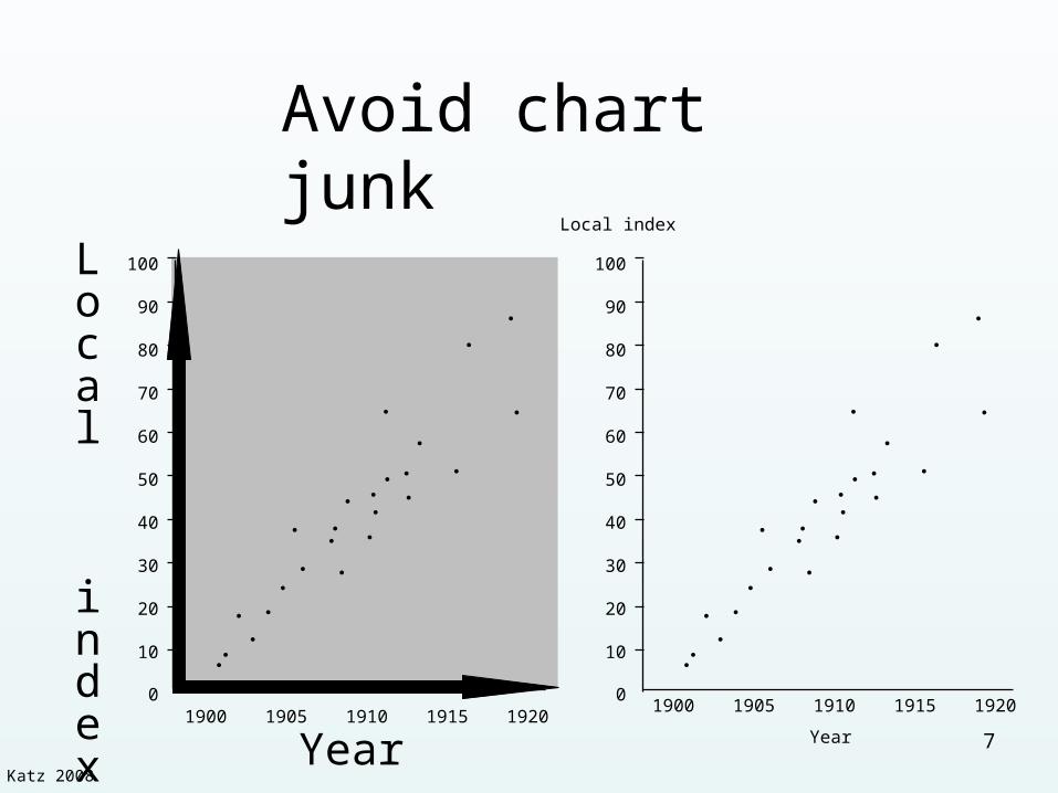
Avoid chart junk
7
Katz 2008
Figure captions
• Reader looks at figures then legends
• Title should explain meaning without need to read manuscript
• Does not need to be a complete sentence
• Like table title, usually in two parts– Descriptive title– Essential details
8
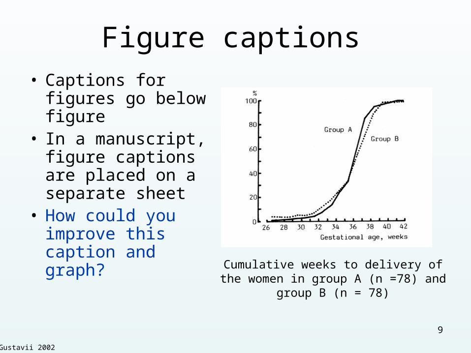
Figure captions• Captions for figures
go below figure• In a manuscript,
figure captions are placed on a separate sheet
• How could you improve this caption and graph?
Cumulative weeks to delivery of the women in group A (n =78) and group B
(n = 78)
9
Gustavii 2002
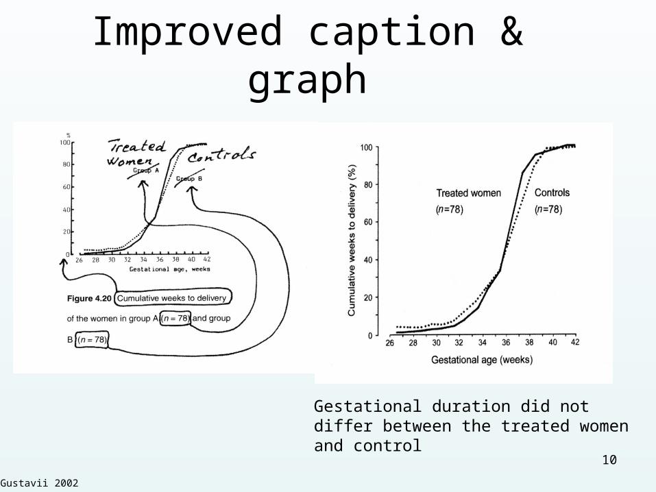
Improved caption & graph
Gestational duration did not differ between the treated women and control
Gustavii 2002
10
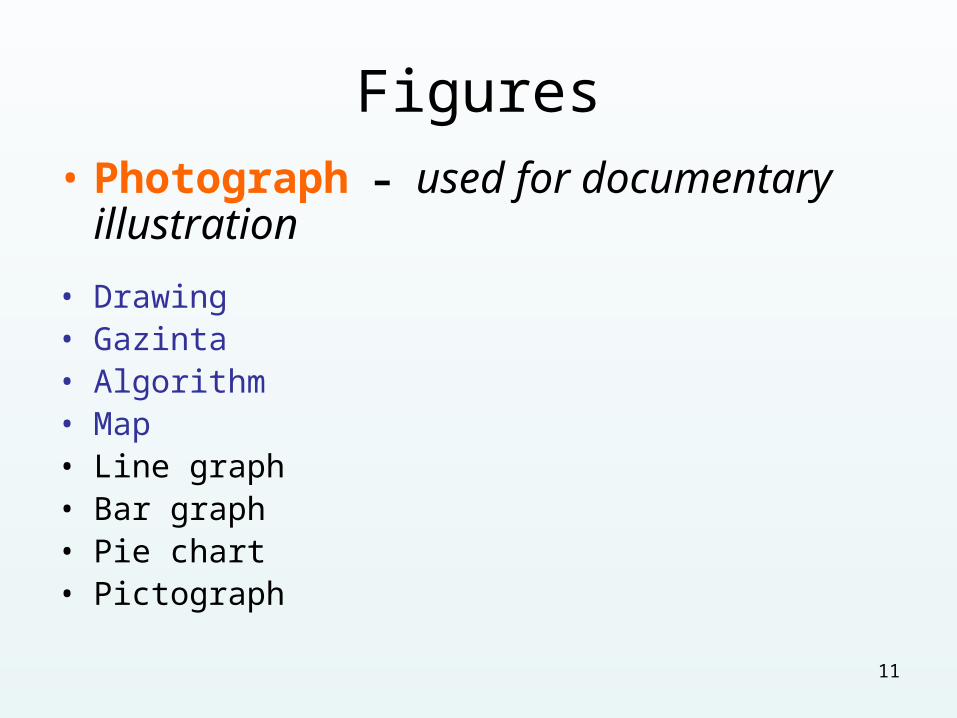
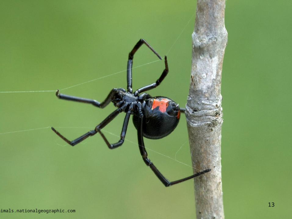
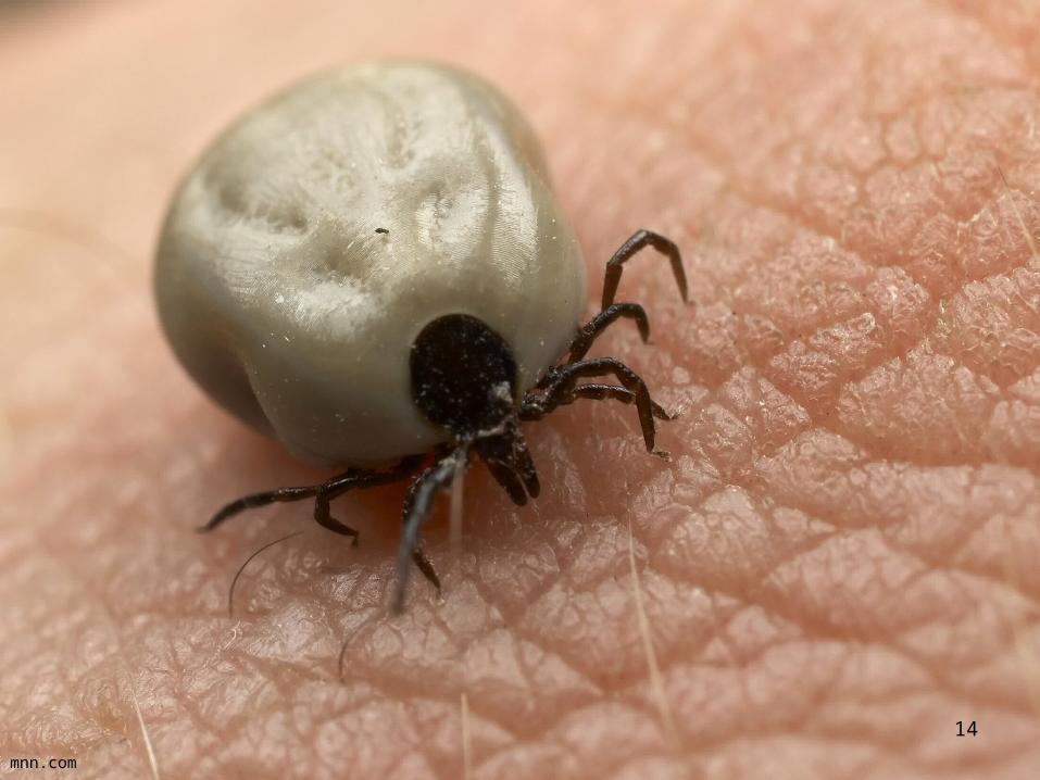
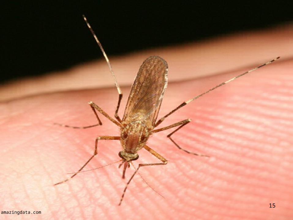
Figures• Photograph – used for documentary
illustration
• Drawing• Gazinta• Algorithm• Map• Line graph• Bar graph• Pie chart• Pictograph
11
Photograph
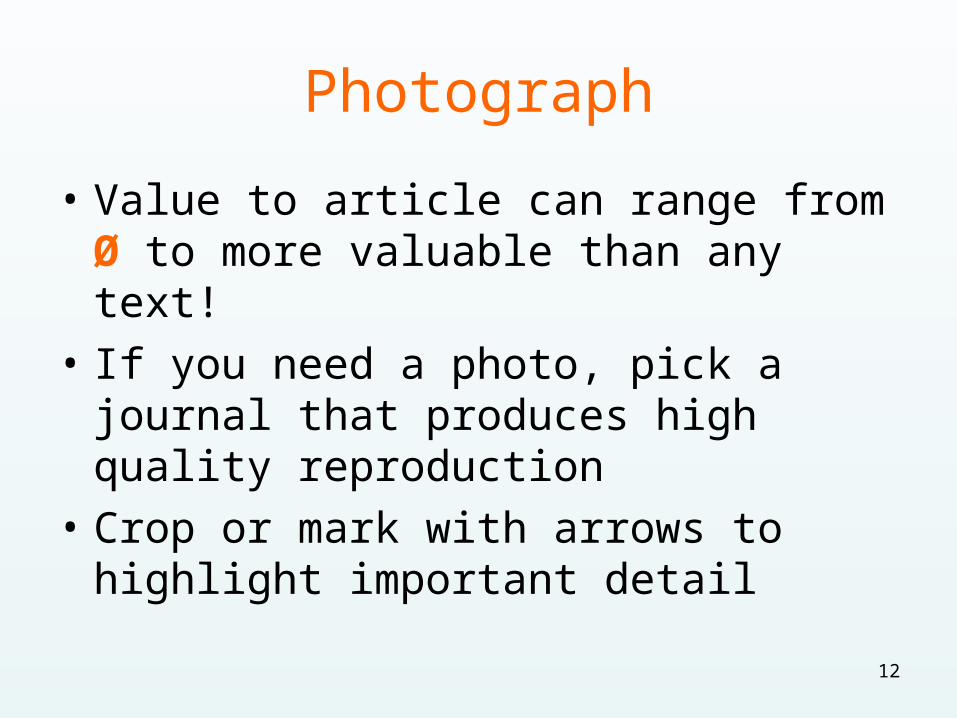
• Value to article can range from Ø to more valuable than any text!
• If you need a photo, pick a journal that produces high quality reproduction
• Crop or mark with arrows to highlight important detail
12
13animals.nationalgeographic.com
14
mnn.com
15amazingdata.com
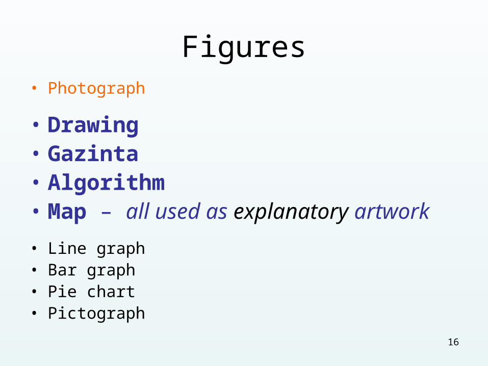
Figures• Photograph
• Drawing• Gazinta• Algorithm• Map – all used as explanatory artwork
• Line graph• Bar graph• Pie chart• Pictograph
16
Drawing
Can show perspective and detail (insides, layers) not possible with a photograph
17

Drawing allows control of detail
18
Jamie Myers
Gazinta
Visuals that show hierarchy, organization or interaction
• Tree gazintas show sub-assemblies of the same relative importance
• Block diagrams are interaction gazintas
19
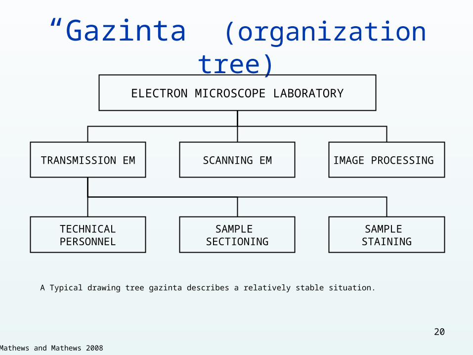
“Gazinta” (organization tree)
ELECTRON MICROSCOPE LABORATORY
TRANSMISSION EM SCANNING EM IMAGE PROCESSING
TECHNICAL PERSONNEL
SAMPLE SECTIONING
SAMPLE STAINING
A Typical drawing tree gazinta describes a relatively stable situation.
20
Mathews and Mathews 2008
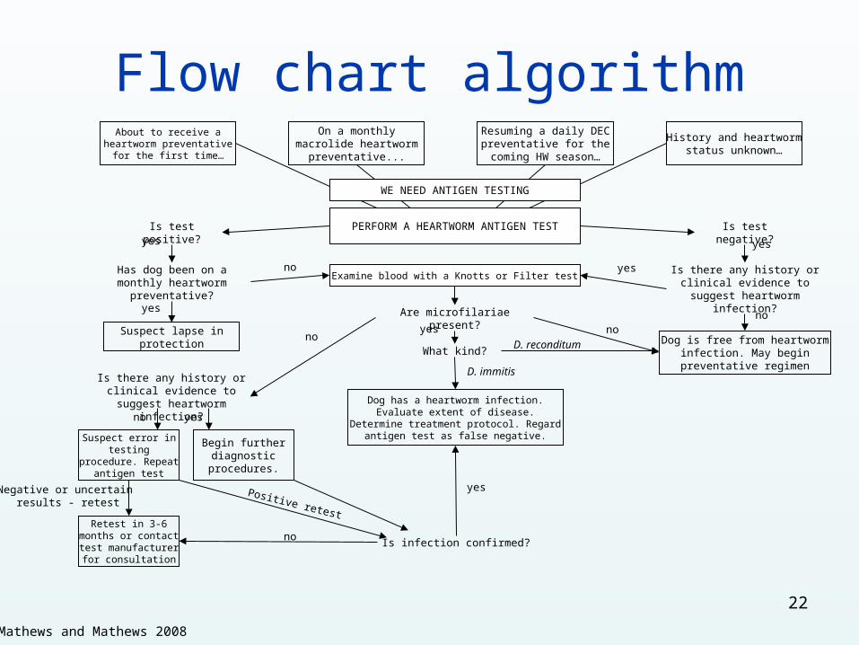
Algorithm
• Flowcharts & taxonomic keys
• Algorithms are illustrations of a means of making a decision by considering only those factors relevant to that decision
• Algorithms are usually easier to follow than the written text equivalent
21
Flow chart algorithmAbout to receive a
heartworm preventative for the first time…
On a monthly macrolide heartworm
preventative...
Resuming a daily DEC preventative for the coming HW season…
History and heartworm status unknown…
PERFORM A HEARTWORM ANTIGEN TEST
WE NEED ANTIGEN TESTING
Is test positive?
Examine blood with a Knotts or Filter testnoHas dog been on a monthly
heartworm preventative?
yes
Suspect lapse in protection
yesIs test negative?
yes
Is there any history or clinical evidence to suggest
heartworm infection?
no
Dog is free from heartworm infection. May begin
preventative regimen
Are microfilariae present?
Is there any history or clinical evidence to suggest
heartworm infection?
no
yes
noyes
What kind?
Dog has a heartworm infection. Evaluate extent of disease. Determine
treatment protocol. Regard antigen test as false negative.
D. immitis
Suspect error in testing procedure.
Repeat antigen test
Begin further diagnostic
procedures.
no yes
Retest in 3-6 months or contact test manufacturer for consultation
Negative or uncertain results - retest
Is infection confirmed?no
yesPositive retest
D. reconditum
22
Mathews and Mathews 2008
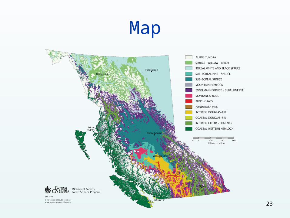
Map
23
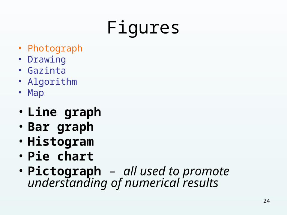
Figures• Photograph• Drawing• Gazinta• Algorithm• Map
• Line graph• Bar graph• Histogram• Pie chart• Pictograph – all used to promote
understanding of numerical results24
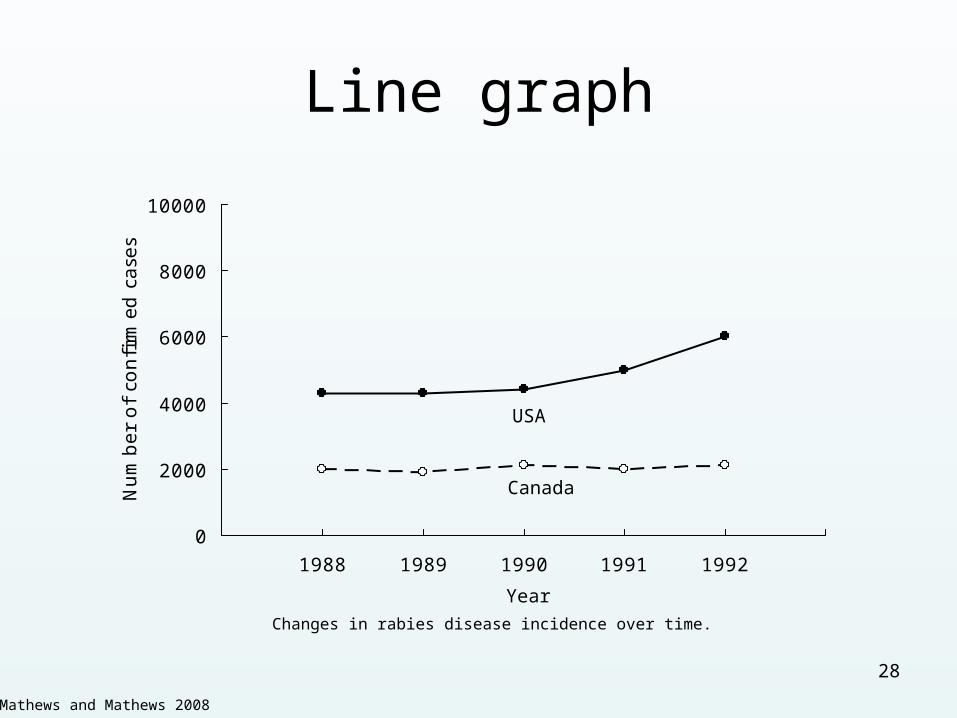
Line graph
Graphs are a good choice when you think that a relationship is more important to the reader than the actual numbers
25
Line graph
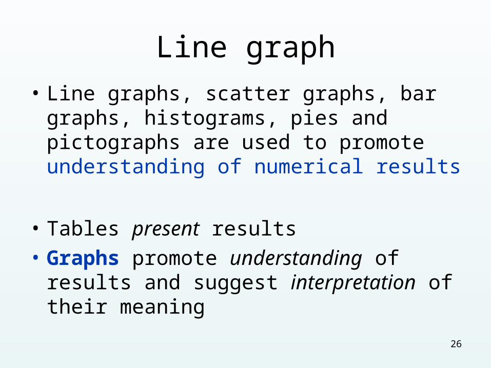
• Line graphs, scatter graphs, bar graphs, histograms, pies and pictographs are used to promote understanding of numerical results
• Tables present results
• Graphs promote understanding of results and suggest interpretation of their meaning
26
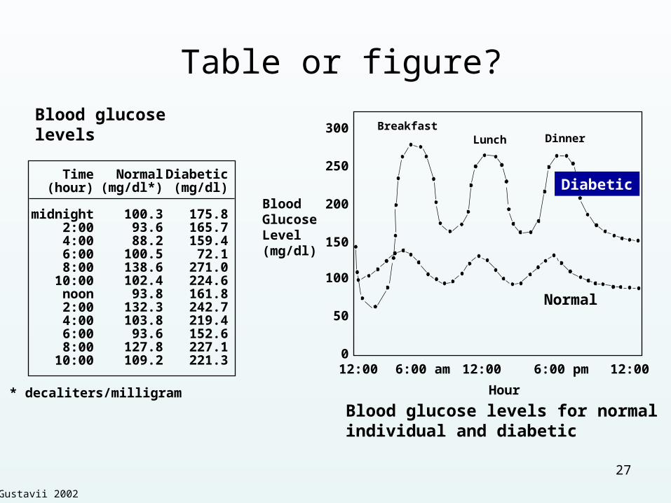
Table or figure?
Time(hour)
midnight2:004:006:008:00
10:00noon2:004:006:008:00
10:00
Normal(mg/dl*)
100.393.688.2
100.5138.6102.4
93.8132.3103.8
93.6127.8109.2
Diabetic(mg/dl)
175.8165.7159.4
72.1271.0224.6161.8242.7219.4152.6227.1221.3
Blood glucose levels
* decaliters/milligram
Blood glucose levels for normal individual and diabetic
Hour
12:00 6:00 am 12:00 6:00 pm 12:00
BloodGlucoseLevel(mg/dl)
300
250
200
150
100
50
0
BreakfastLunch Dinner
Normal
Diabetic
27
Gustavii 2002
Line graph
0
2000
4000
6000
8000
10000
1988 1989 1990 1991 1992
Num
ber
of
confirm
ed c
ases
USA
YearChanges in rabies disease incidence over time.
Canada
28
Mathews and Mathews 2008
-20
0
20
40
60
80
100
0 30 60 90 120 150
Right eye
Left eye
Minutes
Pup
il d
iam
ete
r (%
cha
nge
)
-20
0
20
40
60
80
100
Minutes
Pup
il d
iam
ete
r (%
cha
nge
) Right eye
Left eye
0 30 60 90 120 150
Tyramine Tyramine
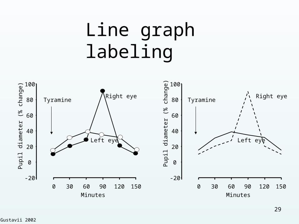
Line graph labeling
29
Gustavii 2002
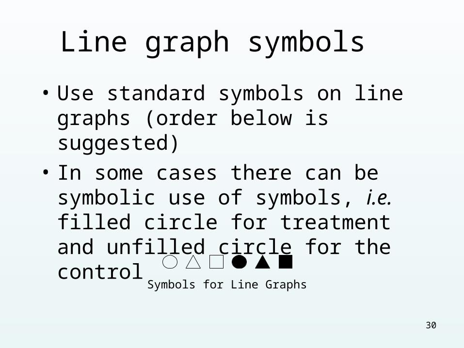
Line graph symbols
• Use standard symbols on line graphs (order below is suggested)
• In some cases there can be symbolic use of symbols, i.e. filled circle for treatment and unfilled circle for the control
Symbols for Line Graphs
30
visible pattern
0
2
4
6
8
10
12
14
16
2
y
0 4 6 8 10 12 14 16x
no visible pattern
0
2
4
6
8
10
12
14
16
2
y
0 4 6 8 10 12 14 16 x
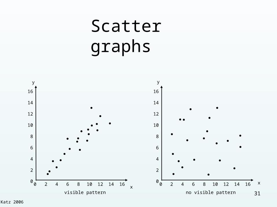
Scatter graphs
31
Katz 2006
Bar graph
• Used to present discrete (unrelated) variables in a forceful way
• Downside is that they present a relatively small amount of information in quite a large space
32
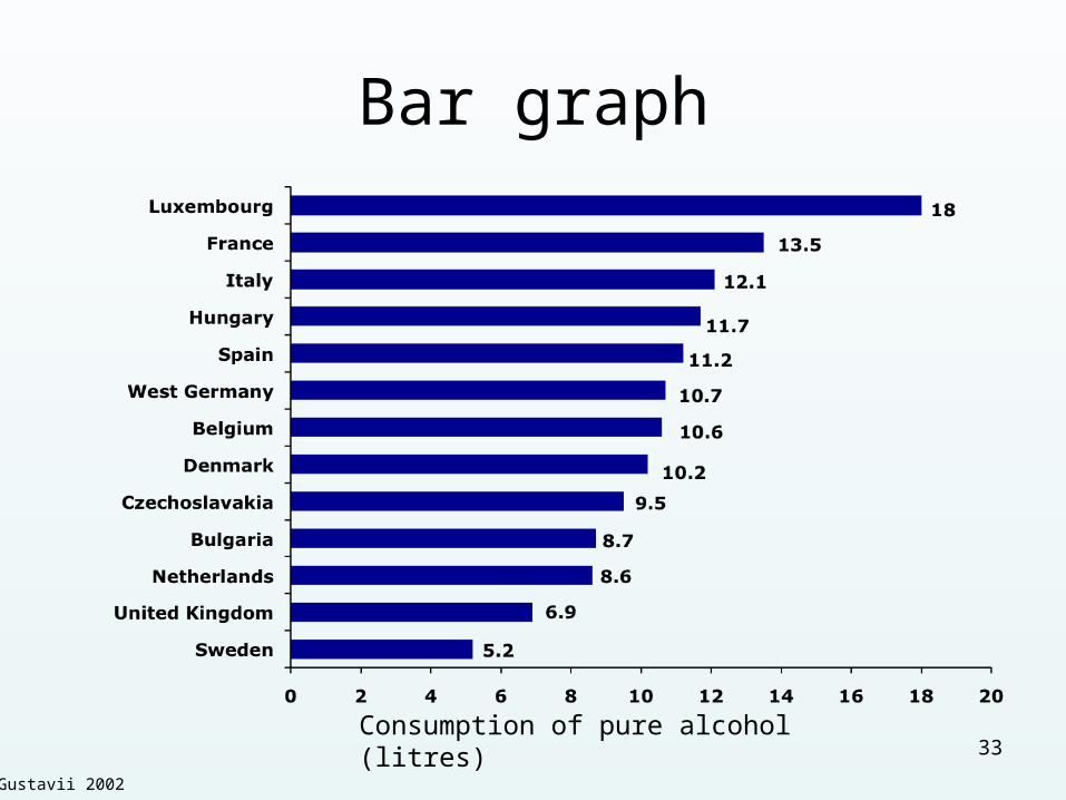
Consumption of pure alcohol (litres)
Bar graph
33
Gustavii 2002
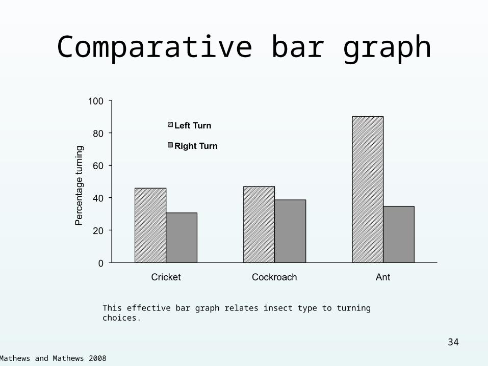
Comparative bar graph
This effective bar graph relates insect type to turning choices.
34
Mathews and Mathews 2008
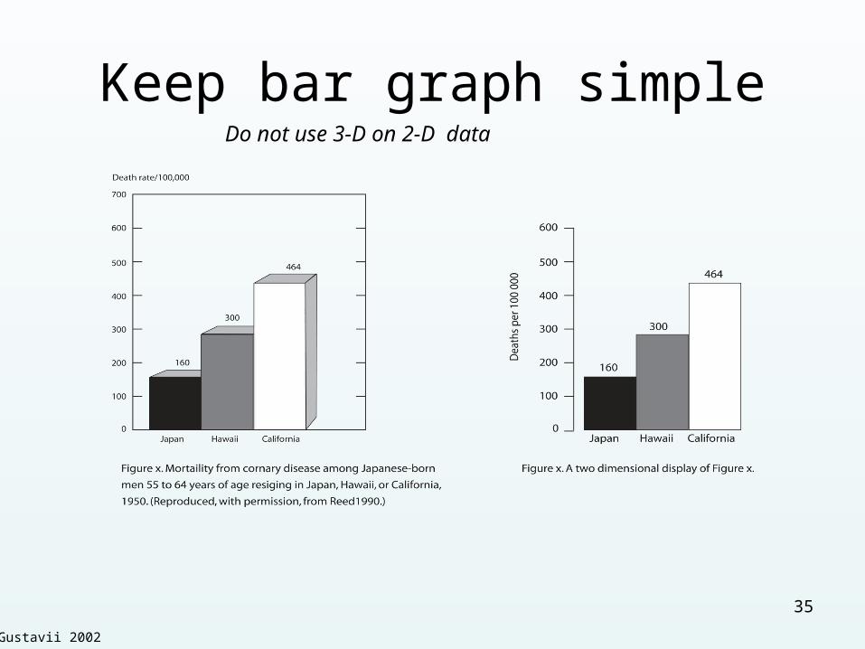
Keep bar graph simpleDo not use 3-D on 2-D data
35
Gustavii 2002
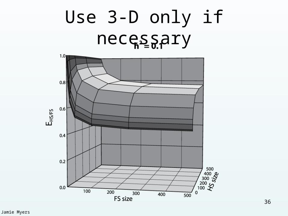
Use 3-D only if necessary
36
Jamie Myers
Histogram
• An estimate of the probability distribution of a continuous variable
• Used to present continuous variables in a forceful way
37
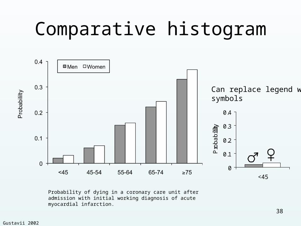
Comparative histogram
Probability of dying in a coronary care unit after admission with initial working diagnosis of acute myocardial infarction.
0
0.1
0.2
0.3
0.4
<45
Pro
ba
bili
lty
Can replace legend with symbols
38
Gustavii 2002
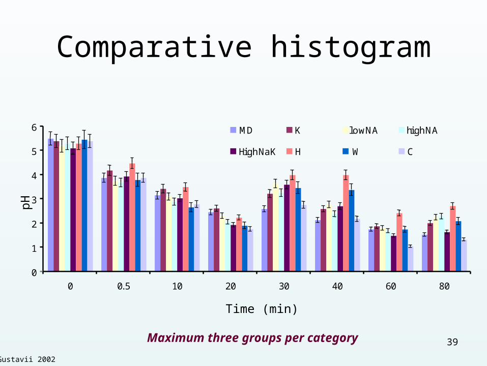
Comparative histogram
Time (min)
pH
0
1
2
3
4
5
6
0 0.5 10 20 30 40 60 80
MD K lowNA highNA
HighNaK H W C
Maximum three groups per category 39
Gustavii 2002
Pie graph
• Good for getting attention
• Show relationship of a number of parts to the whole
• Arrange segments in size order with largest at 12 o’clock
• Downside is that you cannot compare areas
40
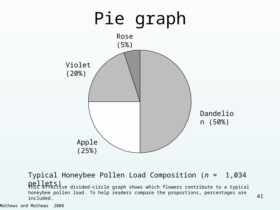
Pie graph
Dandelion (50%)
Apple (25%)
Violet (20%)
Rose (5%)
Typical Honeybee Pollen Load Composition (n = 1,034 pellets)
This effective divided-circle graph shows which flowers contribute to a typical honeybee pollen load. To help readers compare the proportions, percentages are included.
41
Mathews and Mathews 2008

Pictograph
Bar graphs made of pictures
42
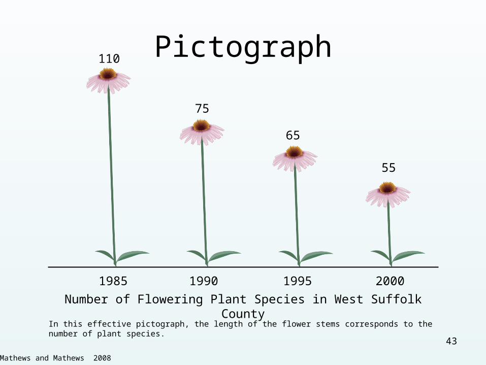
Pictograph
Number of Flowering Plant Species in West Suffolk County
1985 1990 1995 2000
110
75
65
55
In this effective pictograph, the length of the flower stems corresponds to the number of plant species.
43
Mathews and Mathews 2008
Numbers and Statistics
44

Numbers and Statistics
45
46
Using statistics
Using statistics properly is a skill
Never be afraid to ask for advice
Dr Tony KozakWednesdays 8:30 – 11:00 amFSC 2027 by appointment [email protected]
47
Descriptive statistics
Usually want to reduce the volume of your data to a few characteristic numbers
These characteristic numbers are descriptive statistics
Certain descriptive statistics are particularly helpful in your Results section
48
49
thingsbiological.wordpress.com
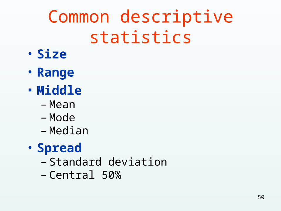
Common descriptive statistics
• Size
• Range
• Middle– Mean– Mode– Median
• Spread– Standard deviation– Central 50%
50
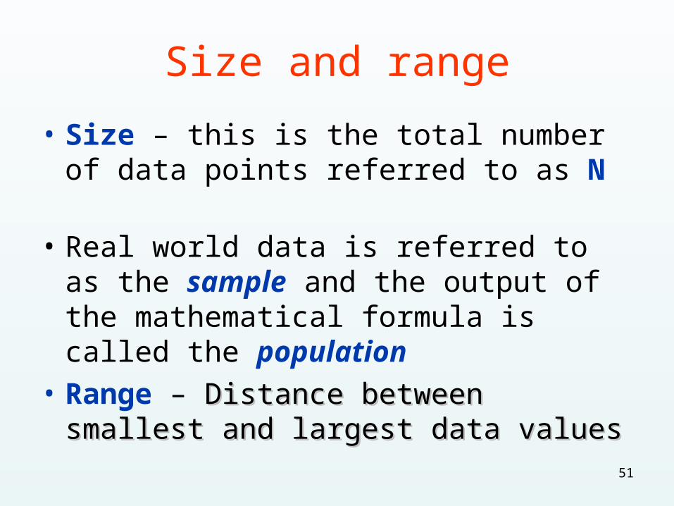
Size and range
• Size – this is the total number of data points referred to as N
• Real world data is referred to as the sample and the output of the mathematical formula is called the population
• Range – Distance between smallest and Distance between smallest and largest data valueslargest data values
51
Middle
• Mean – Average data value
• Mode – Data value that occurs most often
• Median – Value such that half the data values are less than this and half are greater
52
Spread
• Standard deviation – Deviation of each data point from the mean
• Large standard deviation means data points are more spread out
• Central 50% – Boundaries in which the middle half of the data points lie when all placed in order
53
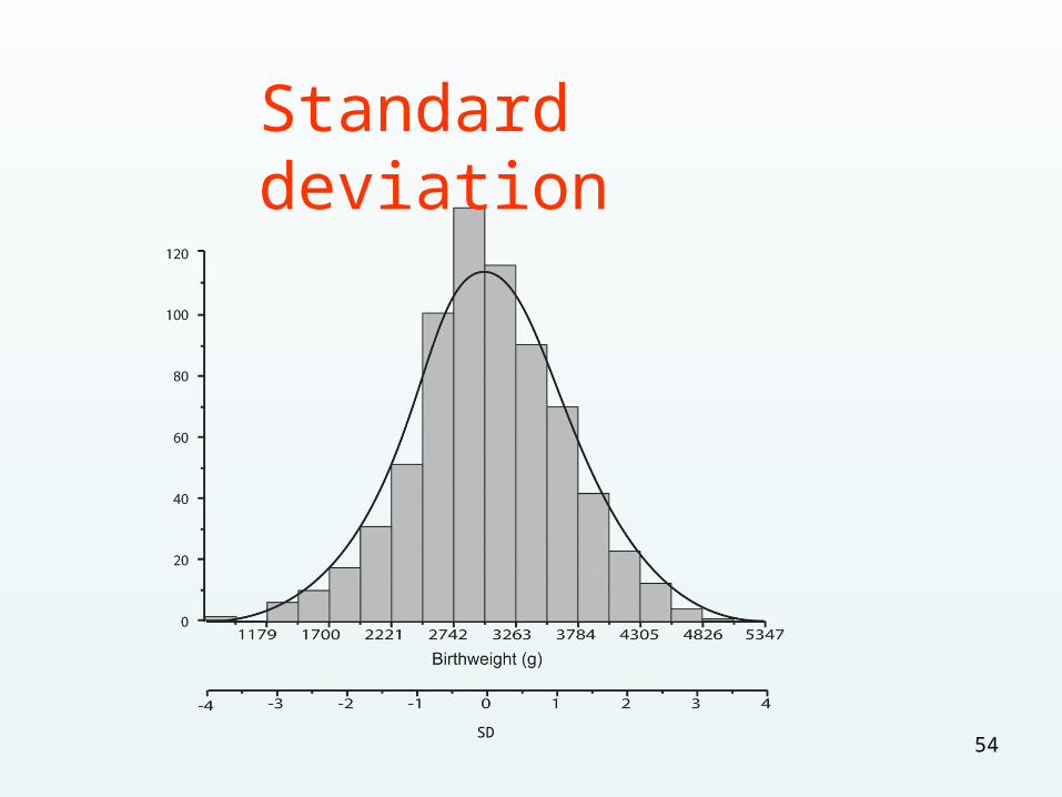
SD
Standard deviation
54
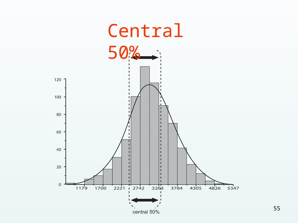
Central 50%
55
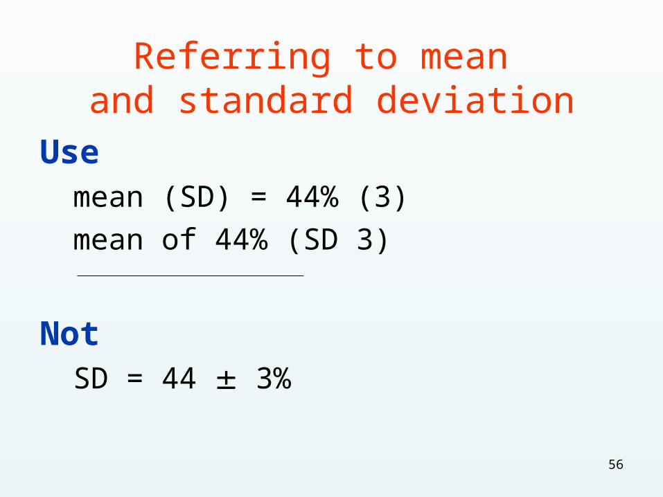
Referring to mean and standard deviation
Use mean (SD) = 44% (3)
mean of 44% (SD 3)
NotSD = 44 3%
56
Standard error or standard deviation?
• Standard error (SE) is not a measure of variability
• Standard error is the standard deviation of a statistic and as such is a measure of precision for an estimate
• However, SE is often used descriptively and must be properly identified to avoid confusion
57
Inferential statistics
• Pure mathematics exists in an abstract universe, parallel to the real world
• Inferential statistics is done in the mathematical universe and infers the identity of the mathematical formula from the real world sample
58
Inferential statistics
• Statistical judgments are made by working on the formula in the mathematical universe
• Inferences are covered in your Discussion
59
Normal distribution
• A curve with a smooth bell shape
• Mean, median and mode have same value
• The exact shape of any normal distribution can be defined with just 2 numbers– Its mean and– Its standard deviation
60
Normal distribution
• In the real world no data set makes a perfect curve with infinite smoothness
• Nevertheless, we frequently call real world data sets “normally distributed”
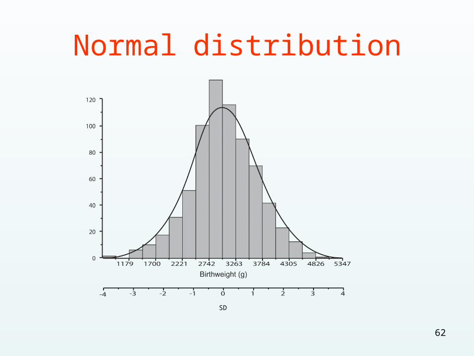
• Many large sets of real world data CAN be well approximated with a normal distribution (baby birth weights). Normal distributions are frequently used in statistical analyses
61
Normal distribution
SD
62
Normal distribution
• Examine your data set carefully
• Look at its shape and do not make any assumptions based on a normal distribution if you are not sure
• Check with a statistician to be certain
63
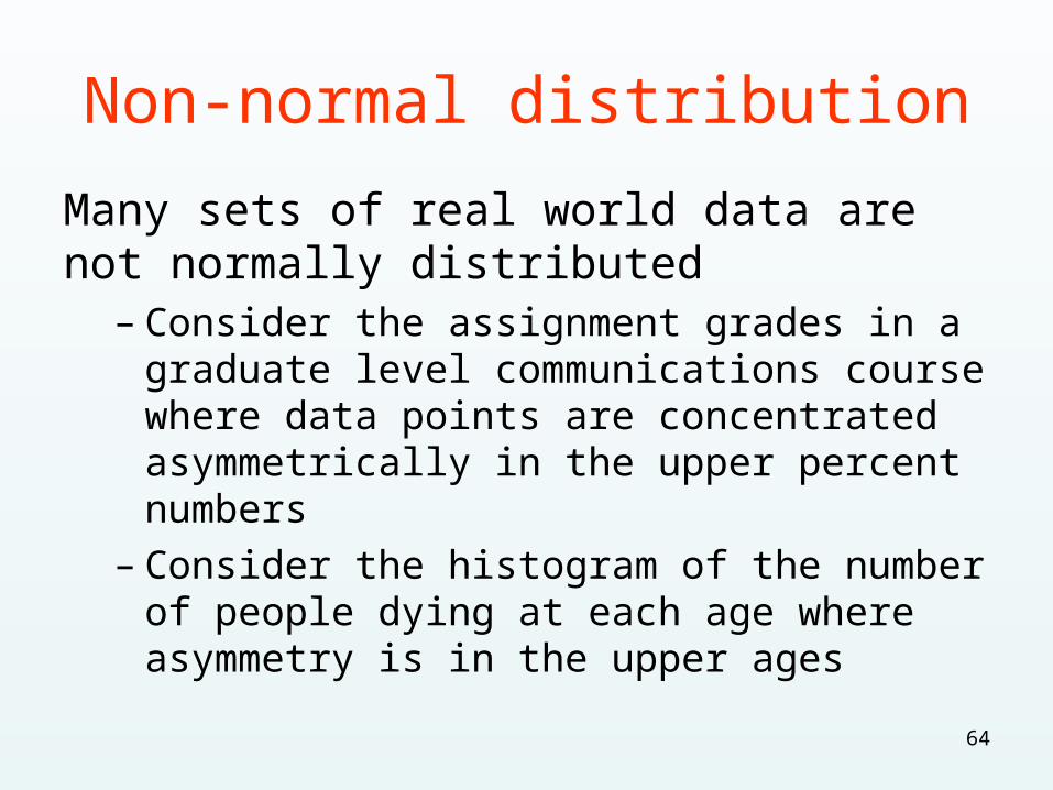
Non-normal distribution
Many sets of real world data are not normally distributed
– Consider the assignment grades in a graduate level communications course where data points are concentrated asymmetrically in the upper percent numbers
– Consider the histogram of the number of people dying at each age where asymmetry is in the upper ages
64
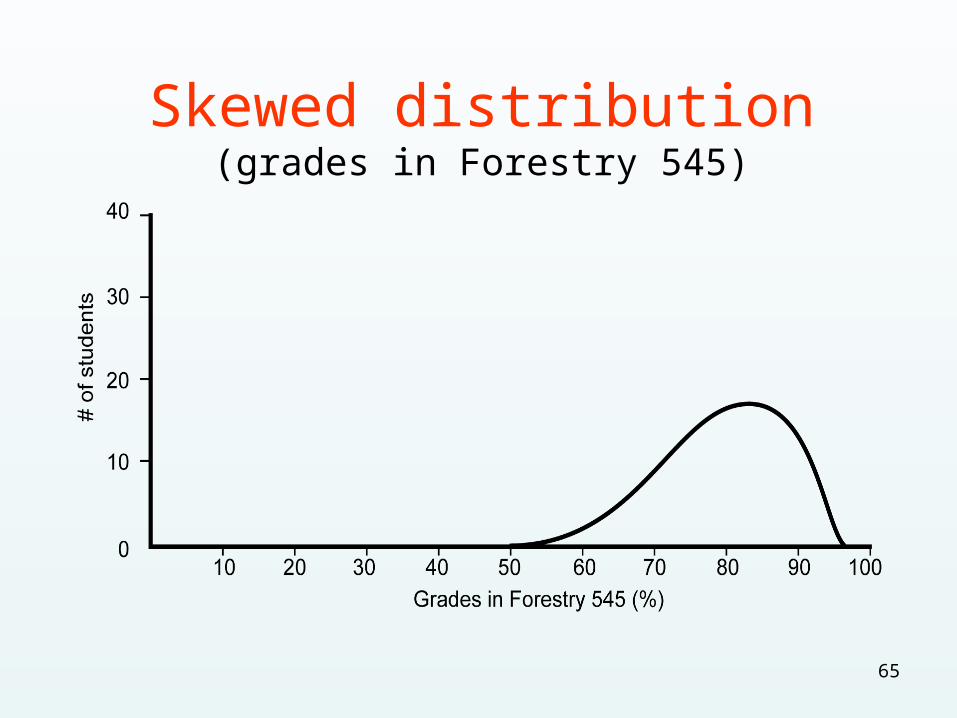
Skewed distribution(grades in Forestry 545)
65
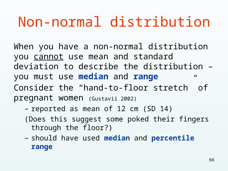
Non-normal distribution
When you have a non-normal distribution you cannot use mean and standard deviation to describe the distribution – you must use median and rangeConsider the “hand-to-floor stretch” of pregnant women (Gustavii 2002)
– reported as mean of 12 cm (SD 14)
(Does this suggest some poked their fingers through the floor?)
– should have used median and percentile range
66
Non-normal distribution
Rule of thumb
If SD is greater than half the mean, the data are unlikely to be normally distributed
Most results in biomedical science are asymmetrically distributed
67
Hypothesis testing
• In hypothesis testing need to specify probability of a type I error or significance level (α) Usually use α = 0.05
• Results from hypothesis testing should include– Test statistic– Degrees of freedom– P value
68
Choosing a significance test
Do not begin with a test in mind
Answer yes/no questions about what you want to assign confidence levels to
Is my data normally distributed?Is my data random?Does my data match someone else’s?Does my data from exp A differ from data set
of exp B?
69
Choosing a significance test
Now pick a significance test that will directly answer your questions using the data in the form that you have generated
Do not be afraid to ask for advice
70
Probability values
• P value is the probability of obtaining a value of test statistic as large as that observed by chance alone
• Do not confuse this P value with the significance level of the test (α)
• Simply stating that a P value was greater or less than a significance level reduces interpretation to a yes or no
71
Probability values
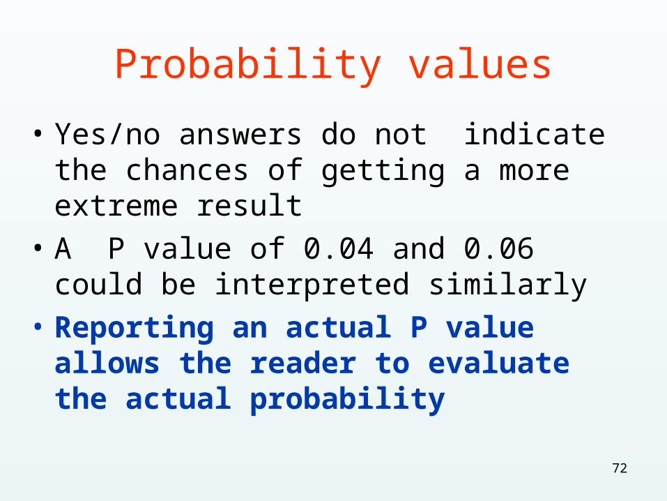
• Yes/no answers do not indicate the chances of getting a more extreme result
• A P value of 0.04 and 0.06 could be interpreted similarly
• Reporting an actual P value allows the reader to evaluate the actual probability
72
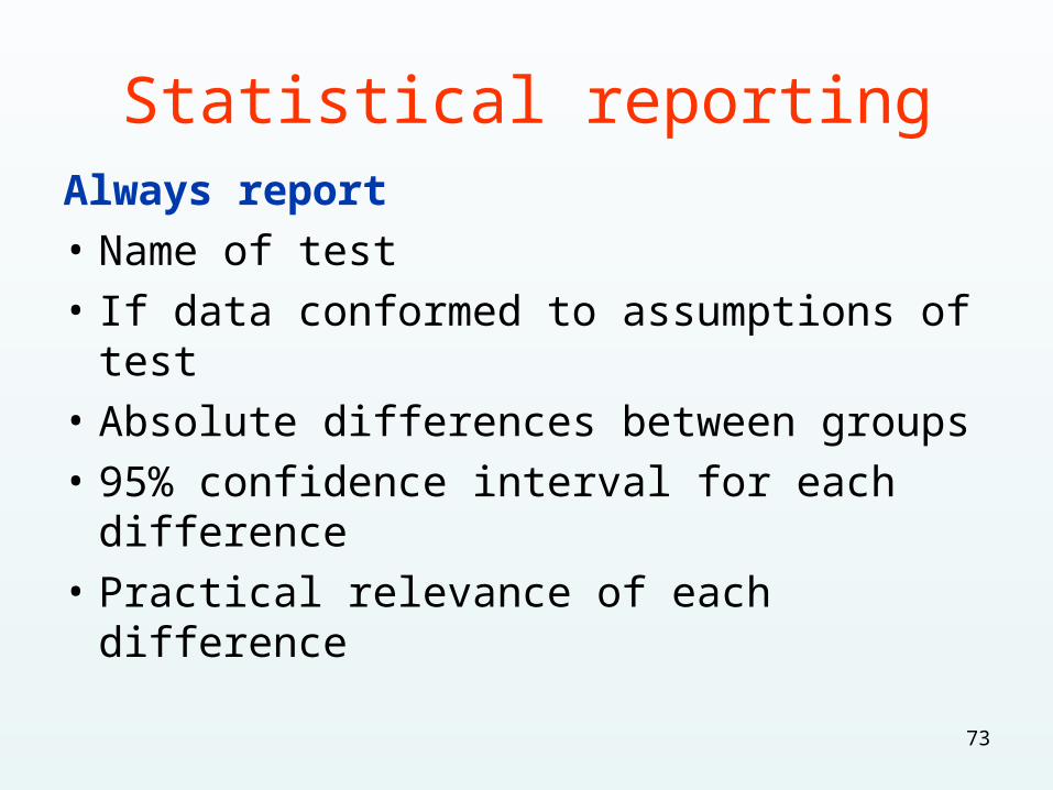
Statistical reportingAlways report
• Name of test
• If data conformed to assumptions of test
• Absolute differences between groups
• 95% confidence interval for each difference
• Practical relevance of each difference
73
Statistical reporting
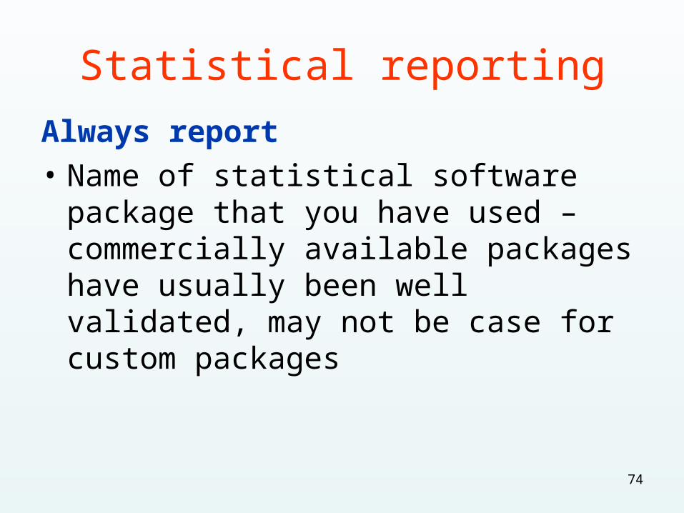
Always report
• Name of statistical software package that you have used – commercially available packages have usually been well validated, may not be case for custom packages
74
Statistical reporting
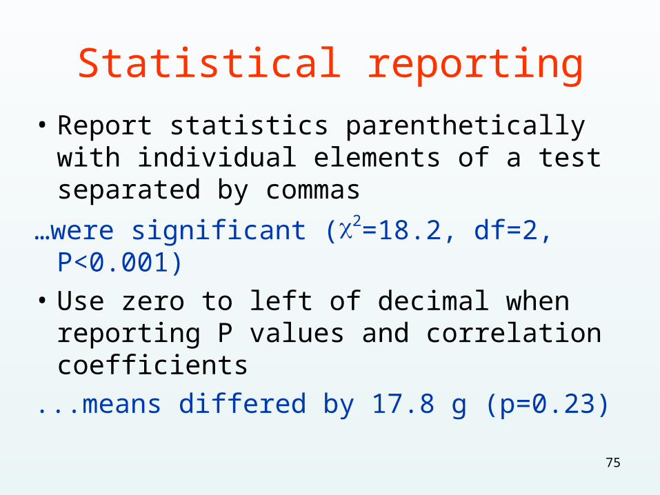
• Report statistics parenthetically with individual elements of a test separated by commas
…were significant (2=18.2, df=2, P<0.001)
• Use zero to left of decimal when reporting P values and correlation coefficients
...means differed by 17.8 g (p=0.23)
75
Statistical reporting
• Do not use more than 3 decimal places when reporting P values
• Use exact values rather than inequalities
• Smallest P value that needs to be reported is p<0.001
76
Statistical reporting
• Statistical methods do not need elaborate presentation – a simple statement of the chosen test and the probability level is usually all that is needed
• Reference a text that details the procedure if you feel that this is necessary
77
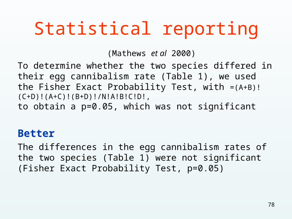
Statistical reporting (Mathews et al 2000)
To determine whether the two species differed in their egg cannibalism rate (Table 1), we used the Fisher Exact Probability Test, with =(A+B)!(C+D)!(A+C)!(B+D)!/N!A!B!C!D!,
to obtain a p=0.05, which was not significant
BetterThe differences in the egg cannibalism rates of the two species (Table 1) were not significant (Fisher Exact Probability Test, p=0.05)
78
Statistical significance & scientific importance
Scientific research yields 2 kinds of significanceScientific
Statistical
Scientific importance is often ignored as it involves some subjectivity
Statistical significance is easy to convey but may lack scientific vigour
79
Statistical significance & scientific importance
A test result may be statistically significant but the difference between the means tested may be so small that it is scientifically irrelevant
Also, the power of a test increases with sample size and large samples may reveal differences that small ones would not
80
Statistical significance & scientific importance
Statistically significant results should always be accompanied by a discussion of the scientific importance of the findings
81
Statistical significance & scientific importance
Drug lowered blood pressure by a mean of8 mm Hg from 100 – 92 mm HgStatistically significant (p<0.05)
Better way to present this is with 95% confidence interval (CI)
Here, CI was 2 – 14 mm HgScientifically important to decrease blood pressure by as much as 14 mm Hg, reduction of 2 mm Hg would not be important
Example from Gustavii 200282
Statistical significance & scientific importance
In this example could have said
Blood pressure was lowered by a mean of 8 mm Hg from 100-92 mm Hg (95% CI=2-14 mm Hg; p=0.02)
P values estimate statistical significance
CI values also estimate scientific importance
When CI is used readers can judge for themselves
83
Potentially problematic statistical terms (CSE 2006)
Random sample implies true randomizationOften confused with “sampling without known bias”Confidence interval or limit better to use interval as limit implies 2 discrete and unchanging valuesStandard deviation better to note as SD rather than S. Does not need sign
84
Potentially problematic statistical terms (CSE 2006)
Standard error of the mean (SE) has little practical value on its own
Use SD (or interpercentile range) not SE to indicate variability in a set of data
Use CI rather than SE as a measure of precision for an estimate
85
Significant digits (CSE 2006)
• Calculated values (means, standard deviations) should be to no more than one significant digit beyond the accuracy of the data
• Only when sample sizes are large (>100) should percentages be expressed to one decimal place
86
Rounding numbers (CSE 2006)
To retain 3 significant digits
If 4th digit is less than 5, leave 3rd unchanged
4.282 becomes 4.28
If 4th digit is greater than 5, increase 3rd by 1
4.286 becomes 4.29
87
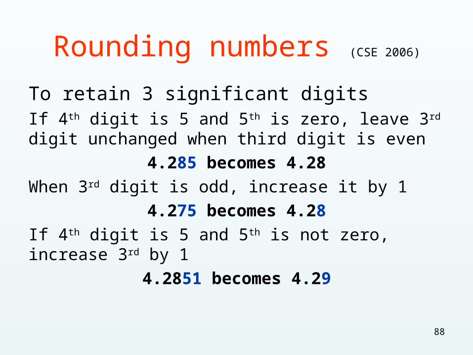
Rounding numbers (CSE 2006)
To retain 3 significant digitsIf 4th digit is 5 and 5th is zero, leave 3rd digit unchanged when third digit is even
4.285 becomes 4.28
When 3rd digit is odd, increase it by 1
4.275 becomes 4.28
If 4th digit is 5 and 5th is not zero, increase 3rd by 1
4.2851 becomes 4.29
88
Numbers and units
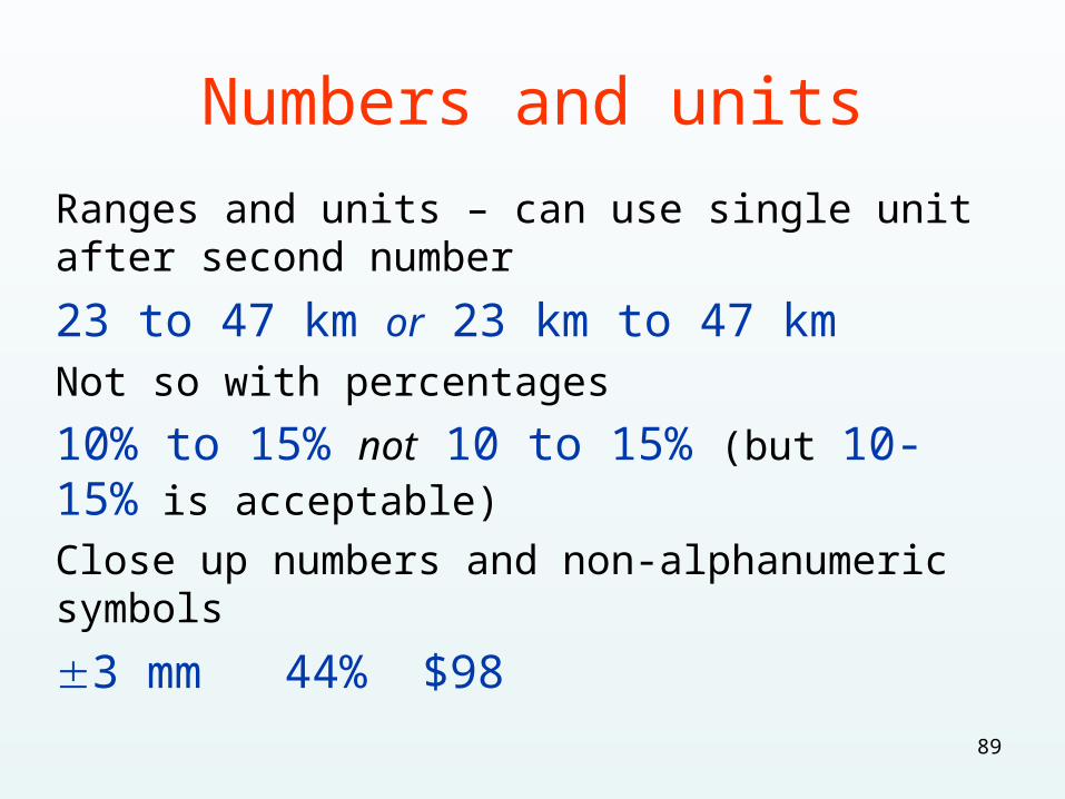
Ranges and units – can use single unit after second number
23 to 47 km or 23 km to 47 kmNot so with percentages
10% to 15% not 10 to 15% (but 10-15% is acceptable)
Close up numbers and non-alphanumeric symbols
3 mm 44% $98
89
Scientific notation (CSE 2006)
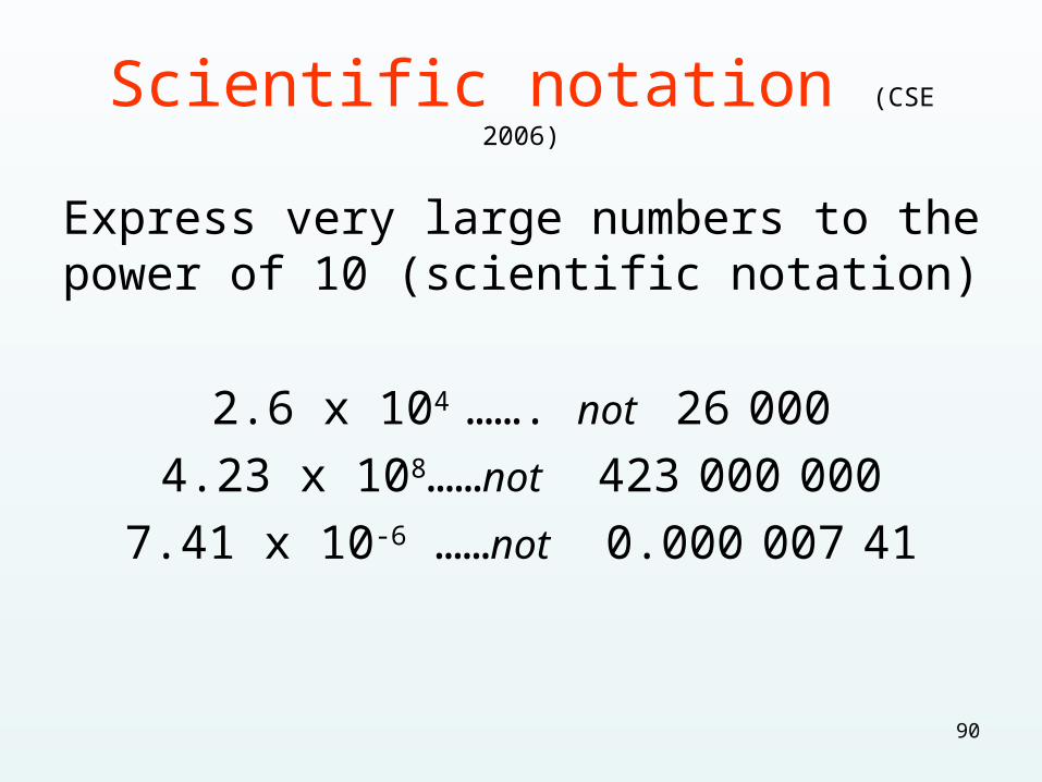
Express very large numbers to the power of 10 (scientific notation)
2.6 x 10⁴ ……. not 26 000
4.23 x 10⁸……not 423 000 000
7.41 x 10⁻⁶ ……not 0.000 007 41
90
Writing numbers
Some rules
Most style manuals now suggest writing out all numbers (not just those <10)
New rule: In 1 of the 19 forest stands…
Still need to spell out numbers at beginning of sentence
91
Writing numbers
Example following this rule:
Three thousand eight hundred and seventy-six seedlings were measured at 8-12 weeks following fertilizer treatment. One hundred and sixty-six (4.3%) were found to have increased height growth.
Correct, but do you find this difficult to grasp?
92
Writing numbers
Better to re-write so that numbers fall somewhere in the middle
Height measurements of 3 876 seedlings at 8-12 weeks following fertilizer treatment showed that 166 (4.3%) had increased growth.
93
Writing numbers
Numbers side by side:
The spiders with dorsal stripes had an average of 257, 112 red and 145 other colours
Need to separate:
The spiders had an average dorsal stripe count of 257, of which 112 were red and 145 were other colours
94
Writing numbers
• American and British practice is to indicate thousands with commas
• However, to avoid confusion with decimal marker, many style manuals recommend the use of a space to mark off thousands
12 345 (not 12,345)
Follow your journal style
95
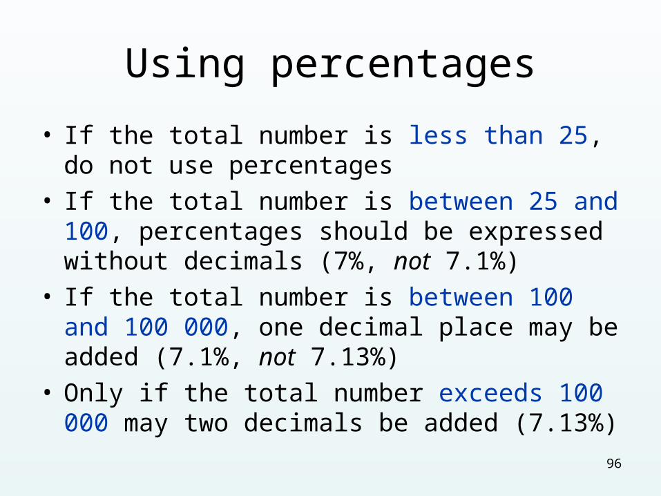
Using percentages
• If the total number is less than 25, do not use percentages
• If the total number is between 25 and 100, percentages should be expressed without decimals (7%, not 7.1%)
• If the total number is between 100 and 100 000, one decimal place may be added (7.1%, not 7.13%)
• Only if the total number exceeds 100 000 may two decimals be added (7.13%)
96
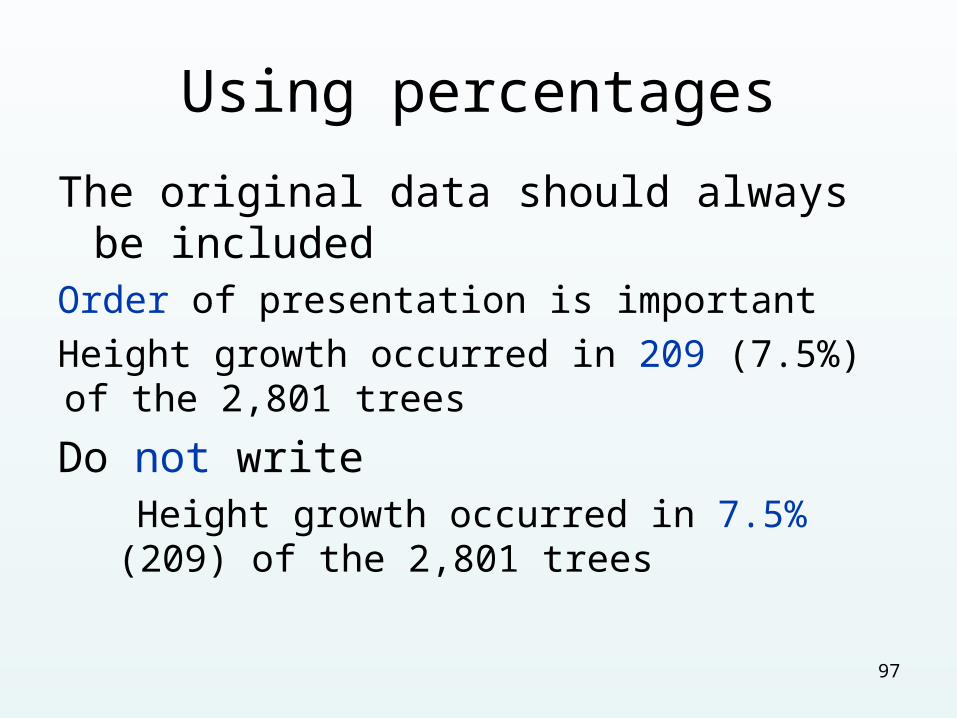
Using percentages
The original data should always be includedOrder of presentation is important
Height growth occurred in 209 (7.5%) of the 2,801 trees
Do not write Height growth occurred in 7.5% (209) of the 2,801 trees
97
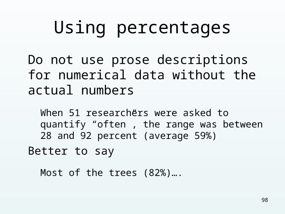
Using percentages
Do not use prose descriptions for numerical data without the actual numbers
When 51 researchers were asked to quantify “often”, the range was between 28 and 92 percent (average 59%)
Better to say
Most of the trees (82%)….
98
Assignments
• Assignment #2 “Abstract” due today
• Assignment #3 “Introduction” due in 2 week’s time – March 18
99