FEDERAL RESERVE BANK OF SAN FRANCISCO

WORKING PAPER SERIES

Restrictions on Risk Prices in Dynamic Term Structure Models

Michael D. Bauer Federal Reserve Bank of San Francisco

March 2016

Working Paper 2011-03 http://www.frbsf.org/publications/economics/papers/2011/wp11-03bk.pdf

The views in this paper are solely the responsibility of the author and should not be interpreted as reflecting the views of the Federal Reserve Bank of San Francisco or the Board of Governors of the Federal Reserve System.

Restrictions on Risk Prices

in Dynamic Term Structure Models∗

Michael D. Bauer†

March 3, 2016

Abstract

Restrictions on the risk-pricing in dynamic term structure models (DTSMs) tighten

the link between cross-sectional and time-series variation of interest rates, and make

absence of arbitrage useful for inference about expectations. This paper presents a new

econometric framework for estimation of affine Gaussian DTSMs under restrictions on

risk prices, which addresses the issues of a large model space and of model uncertainty

using a Bayesian approach. A simulation study demonstrates the good performance

of the proposed method. Data for U.S. Treasury yields calls for tight restrictions on

risk pricing: only level risk is priced, and only changes in the slope affect term pre-

mia. Incorporating the restrictions changes the model-implied short-rate expectations

and term premia. Interest rate persistence is higher than in a maximally-flexible model,

hence expectations of future short rates are more variable—restrictions on risk prices

help resolve the puzzle of implausibly stable short-rate expectations in this literature.

Consistent with survey evidence and conventional macro wisdom, restricted models at-

tribute a large share of the secular decline in long-term interest rates to expectations of

future nominal short rates.

Keywords: no-arbitrage, prices of risk, term premium, Markov-chain Monte Carlo, model

selection

JEL Classifications: C52, E43, G12

∗Previous versions of this paper were circulated under the titles “Bayesian Estimation of Dynamic TermStructure Models under Restrictions on Risk Pricing” and “Term Premia and the News.” The views in thispaper do not necessarily reflect those of others in the Federal Reserve System.†Federal Reserve Bank of San Francisco, michael.bauer@sf.frb.org

1 Introduction

Policymakers and academic researchers are keenly interested in estimating the expectations

and term premium components in long-term interest rates. Dynamic term structure models

(DTSMs), which impose absence of arbitrage, are widely used for this purpose. The no-

arbitrage assumption can be powerful if it creates a link between the cross-sectional variation

of interest rates and their time-series variation, but it only does so if the risk adjustment

is restricted. This paper provides an econometric framework for estimating DTSMs under

restrictions on risk prices. The results show that making use of no-arbitrage in this way

changes the implications for expectations and term premia.

Estimation of term premia amounts to estimation of expectations of future short-term

interest rates. Doing so with only time-series information is extremely difficult, because the

very high persistence of interest rates leads to large statistical uncertainty and small-sample

bias.1 The no-arbitrage assumption in DTSMs can alleviate these problems. Because it

requires that the cross section of interest rates reflects forecasts of future short rates, allowing

for a risk adjustment, the cross-sectional information can potentially help to pin down the

unobserved expectations. However, the risk adjustment loosens this connection between cross-

sectional and dynamic properties. Absent any restrictions on the risk pricing, such as in

a maximally-flexible model, the cross section provides no information at all for estimating

the time-series parameters (Joslin et al., 2011)(henceforth JSZ). Notably, almost all existing

DTSMs impose only few or no risk-price restrictions, and effectively make little use of no-

arbitrage. Consequently, these DTSMs suffer from the same problems as time-series models,

and typically imply implausibly fast mean reversion and puzzling term premium behavior

(Bauer et al., 2012; Kim and Orphanides, 2012).

Choosing restrictions on the parameters that determine the risk adjustment is difficult for

at least two reasons: First, model selection is complicated by the large number of possible

restrictions. Even in a small model with only three risk factors, and focusing only on zero

restrictions on risk-price parameters, there are 212 models to choose from. Brute-force esti-

mation of this amount of highly nonlinear models is at the very least inconvenient and in

most cases infeasible. The second challenge is that the choice of restrictions entails model un-

certainty, which is particularly problematic in the DTSM context. Equally plausible models,

which differ only little in terms of risk-price restrictions, often reveal dramatically different

short-rate expectations and term premia (Kim and Orphanides, 2012; Bauer and Neely, 2014).

1Many studies have noted this problem, including Rudebusch (2007), Cochrane and Piazzesi (2008), Duffeeand Stanton (2012), and Kim and Orphanides (2012). Intuitively, the mean and the speed of mean reversionof interest rates are hard to estimate because we observe only very few mean reversions.

1

This paper introduces a Bayesian econometric framework that overcomes these challenges.

The framework relies on Markov chain Monte Carlo (MCMC) methods to estimate affine

Gaussian DTSMs with risk price restrictions. Model selection does not require separate es-

timation of every single possible model specification because the MCMC samplers visit only

plausible models and do not waste time in other areas of the model space. Model uncertainty

is dealt with by means of Bayesian Model Averaging (BMA). The key methodological con-

tribution is to develop model-selection samplers for DTSM estimation. I use the insight that

this model-selection problem resembles variable selection in multivariate regressions, and I

adapt existing variable-selection samplers to the problem at hand. The paper and an Online

Appendix provide sufficient details for researchers to easily implement this framework on their

own for yield-curve analysis.2

Bayesian estimation of DTSMs has often been found problematic, with most MCMC sam-

plers displaying very slow convergence and requiring a lot of tuning.3 The reason is that pa-

rameters enter the likelihood in a highly nonlinear fashion, which requires various Metropolis-

Hastings (MH) steps that are often inefficient. A separate contribution of this paper is to

substantially simplify Bayesian DTSM estimation. I show that risk price parameters, which

are crucial for determining the model’s economic implications, can be sampled directly from

their conditional posterior (i.e., using a Gibbs step), because their conditional likelihood func-

tion corresponds to a restricted VAR. I am also able to sample the other parameters very

efficiently using tailored MH steps which do not require tuning. The resulting sampling algo-

rithms are very fast and display excellent convergence properties.4

The results of Bayesian model selection are generally sensitive to the priors, so a key

question is how to choose the prior dispersion of the risk-price parameters. I construct a prior

that is similar in spirit to Zellner’s g-prior. Only one easily interpretable hyperparameter, g,

controls the prior dispersion of the risk-price parameters. I choose a plausible baseline value

of g, informed by common rules-of-thumb, and assess the sensitivity of the model selection

results to changes in g by orders of magnitude.

Because of the novelty of the methodology, it is important to verify that it works in

simulated data. To this end, I apply the estimation method to data that is simulated from a

known model.5 The econometric framework performs well in recovering the zero restrictions

on risk prices and the estimated risk-price parameters. More importantly, the simulation

2The estimation code, written in R, is available from the author upon request.3Examples are Ang et al. (2007, 2011); see Chib and Ergashev (2009) for further discussion.4Chib and Ergashev (2009) and Chib and Kang (2014) have also constructed efficient samplers for MCMC

samplers for DTSM estimation. They take a different route by imposing strong prior restrictions.5My approach is similar to that of George et al. (2008), who also use repeated simulations to assess the

accuracy of their Bayesian method for VAR estimation under parameter restrictions.

2

study shows that estimation under risk-price restrictions accurately infers the true persistence

of interest rates and the volatility of short-rate expectations and term premia. In contrast,

estimation of an unrestricted model leads to persistence that is too low, short-rate expectations

that are too stable, and term premium estimates that are excessively volatile.

The framework is then applied to monthly U.S. Treasury yields over the period from 1990

to 2007, a sample that was studied by JSZ and others. The data call for tight restrictions on

the market prices of risk, in contrast to most models in this literature, and even favor a model

in which only one out of twelve risk-price parameters is unrestricted. This is a fortunate out-

come, because it means that the connection between time-series variation and cross-sectional

variation is relatively tight, which makes no-arbitrage particularly useful. Posterior inference

about the pricing of risks in Treasury markets suggests that level risk is priced but slope and

curvature risks are not, consistent with the finding of Cochrane and Piazzesi (2008). Fur-

thermore, level risk appears to be time-varying and driven predominantly by changes in the

slope of the yield curve, consistent with evidence going back to Fama and Bliss (1987) and

Campbell and Shiller (1991). Notably, the only unrestricted parameter in the favored model

is the one that captures the sensitivity of level risk to changes in the slope. These results

imply that most existing DTSMs allow for deviations from the expectations hypothesis in a

much too general way.

Incorporating these restrictions into an otherwise standard DTSM substantially alters the

economic implications. First and foremost, they change the VAR dynamics of the model,

increasing its persistence relative to a maximally-flexible model. The intuition is that interest

rates are extremely persistent under the risk-neutral (Q) probability measure—far-ahead for-

ward rates are not constant—and the risk-price restrictions pull up the persistence under the

real-world (P) probability measure. As a consequence of the higher persistence, long-horizon

expectations of future short-term interest rates are more variable in the restricted models.

Estimated term premia, which are the difference between long-term rates and expected future

short-term rates, are typically more stable. This finding is particularly noteworthy because

the DTSM literature has long been puzzled by artificially stable expectations and overly vari-

able term premia, see Kim and Orphanides (2012)6 and others. My estimates show that when

DTSMs are estimated under the appropriate risk-price restrictions, this long-standing puzzle

is at least partially resolved.

Risk-price restrictions change our interpretation of the evolution of interest rates over

certain historical episodes, in particular of the secular decline in long rates over the last two

decades. Conventional DTSMs typically explain this by substantial declines in term premia

6An early working paper version of Kim and Orphanides (2012) already noted the puzzling stability offar-ahead short-rate expectations in 2005.

3

and imply only a small role for short-rate expectations. In contrast, restricted models attribute

a more important role to a declining expectations component. The finding that expectations

of short-term interest rates have decreased over the 1990’s and 2000’s is consistent with the

sizable declines in survey-based expectations of inflation and policy rates documented by

Kozicki and Tinsley (2001), Kim and Orphanides (2012), and others. On the other hand,

the common finding that declining term premia explained the behavior of yields during the

conundrum period of 2004 and 2005 appears robust.

Model uncertainty is an important but often-ignored factor when DTSMs are used to

analyze the yield curve and to estimate term premia. Some uncertainty about the risk-

price restrictions remains, and small changes to these restrictions can substantially alter the

economic implications. Therefore it is important to calculate the objects of interest using

BMA, which reveals that the uncertainty is quite significant. These results strongly caution

against the common approach of conditioning on one specific DTSM when studying term

premia.7

A key established fact in the yield curve literature is that excess bond returns are strongly

predictable (e.g., Cochrane and Piazzesi, 2005). Since the preferred model specifications in

this paper imply tightly restricted risk pricing, the question arises whether these models can

reproduce the strong predictability of bond returns. The paper shows that they can: the

model-implied excess return predictability in small simulated samples is very similar to that

in actual interest rate data.

Only few other studies systematically impose restrictions on risk prices in DTSMS. In

earlier work, Cochrane and Piazzesi (2008) derive a specific set of restrictions from a prior re-

gression analysis of return predictability, and impose that all variation in term premia is driven

by their tent-shaped return-forecasting factor. JSZ test one specific reduced-rank restriction

on risk-pricing within their canonical model. In independent and parallel work, Joslin et al.

(2014) estimate their macro-finance DTSM under all possible zero restrictions on risk-price

parameters, and select one specification on the basis of information criteria. My approach does

not require brute-force estimation of every model, delivers intuitively interpretable posterior

model probabilities, and addresses the issue of model uncertainty, which is paramount in the

context of DTSM estimation.

7Examples of studies that use only one specific restricted DTSM for studying term premia are Cochraneand Piazzesi (2008) and Joslin et al. (2014).

4

2 Econometric framework

This section lays out the model specification and the methodology for estimation and model

selection.

2.1 Dynamic Term Structure Model

The models used in this paper belong to the class of affine Gaussian DTSMs, a mainstay of

modern finance.8 Denote by Xt the (N × 1) vector of risk factors, which represents the new

information that market participants obtain at time t. Assume that Xt follows a first-order

Gaussian vector autoregression (VAR) under the physical (real-world) probability measure P,

Xt = µ+ ΦXt−1 + Σεt, (1)

with εt ∼ N(0, IN), Σ lower triangular, and E(εrεs′) = 0, r 6= s. The one-period interest rate

rt is an affine function of the factors,

rt = δ0 + δ′1Xt. (2)

Estimation will be carried out using monthly data, so rt is the one-month interest rate. Assum-

ing absence of arbitrage, there exists a risk-neutral probability measure, denoted by Q, which

prices all financial assets. The stochastic discount factor (SDF), which defines the change of

probability measure between P and Q, is specified as exponentially affine,

− logMt+1 = rt +1

2λ′tλt + λ′tεt+1, (3)

with the (N × 1) vector λt, the market prices of risk, being an affine function of the factors,

λt = Σ−1(λ0 + λ1Xt). (4)

This is the essentially-affine risk-price specification of Duffee (2002). The risk prices λt measure

the additional expected return required per unit of risk in each of the shocks in εt. Consider

how the expected excess return of an n-period bond rate depends on risk prices:

Et(rx(n)t+1) +

1

2V art(rx

(n)t+1) = λ′tCov(εt+1, rxt+1). (5)

8It should be noted that extensions of the ideas in this paper to other classes of DTSMs are easily possible.

5

The risk premium equals the prices of risk times the quantities of risk (the covariances). In a

Gaussian model, the covariances are constant, and the only source of time-variation in term

premia are changes in the market prices of risk.9

Under the above assumptions the risk-neutral dynamics (see Online Appendix A) are given

by

Xt = µQ + ΦQXt−1 + ΣεQt , (6)

where εQtQ∼ N(0, Ik), EQ(εQr ε

Qs′) = 0, r 6= s, and the parameters describing the physical and

risk-neutral dynamics are related in the following way:

µQ = µ− λ0, ΦQ = Φ− λ1. (7)

In this model, yields are affine in the state variables. Denoting the J model-implied (fitted)

yields by Yt, we have

Yt = A+BXt, (8)

where the J-vector A and the J × N -matrix B contain the model-implied loadings of yields

on risk factors, given in Online Appendix B. These are determined by the parameters δ0, δ1,

µQ, ΦQ, and Σ.

To achieve econometric identification, normalizing restrictions are needed. A DTSM is

canonical if it is maximally flexible, subject only to these normalizing restrictions. I use

the canonical form of JSZ, in which the risk factors are linear combinations of yields, and all

normalizing restrictions are imposed on µQ and ΦQ. Formally, Xt = WYt for aN×J matrixW .

The free parameters are: φQ, an N -vector containing the eigenvalues of ΦQ (which are assumed

to be real, distinct, and less than unity), kQ∞, a scalar that determines the unconditional Q-

mean of the short rate10, the risk-price parameters (λ0, λ1), and Σ. JSZ detail how µQ, ΦQ, δ0,

and δ1 are calculated from these parameters and W . The parameterization here includes λ0

and λ1, instead of µ and Φ, because the focus is on inference about these risk-price parameters.

Since interest lies in inference about the prices of risk associated with shocks to Xt, it is

convenient that Xt is not an arbitrary latent state vector but a specific linear combinations of

yields. I take the risk factors Xt as the first three principal components (PCs) of the observed

yields. That is, W contains the loadings of the first three PCs of observed yields, which

correspond to level, slope, and curvature of the yield curve and are sufficient to capture most

of the variation in the yield curve (Litterman and Scheinkman, 1991). This choice of risk

9See Online Appendix G for the details on model-implied excess bond returns and equation (5).10In models that are stationary and have distinct eigenvalues under Q we have for rQ∞ the risk-neutral mean

of the short rate rQ∞ = kQ∞/(1 − λQ1 )—see JSZ, p. 934. Conveniently, the value of kQ∞ that maximizes the

likelihood function for given values of λQ and Σ can be found analytically.

6

factors facilitates an economic interpretation of the prices of risk.

The observed bond yields used for estimation are Yt = Yt + et, where et is a vector of

measurement errors that is iid normal. Measurement errors are included because an N -

dimensional factor model cannot perfectly price J > N yields. I assume that Xt is observable,

i.e., that the N linear combination of yields in W are priced exactly by the model. This

assumption simplifies the estimation somewhat but could be relaxed.11 It implies Xt = WYt =

WYt and Wet = 0 so that there are effectively only J −N independent measurement errors.

Writing W⊥ for a basis of the null space of W (e.g., the loadings of the remaining J−N PCs),

the measurement error assumption is that W⊥et ∼ N(0, σ2eIJ−N).

2.2 No-arbitrage and restrictions on risk prices

Absence of arbitrage requires the consistency of the time-series dynamics of interest rates with

their cross-sectional behavior, allowing for a risk adjustment. The risk-price parameters λ0

and λ1 in equation (7) determine this risk adjustment and the behavior of term premia. Under

the (weak) EH, λ1 is zero, and term premia are constant. In a maximally-flexible model, all

elements of λ0 and λ1 are unrestricted. The point of this paper is that the “truth” likely lies

somewhere between these two extremes.

Without constraints on the risk pricing, the no-arbitrage assumption is not very restrictive,

as it only requires that the yield loadings be consistent with some values for µQ and ΦQ.12

However, if λ0 and λ1 are restricted, then the information in the cross section of yields is

used to pin down the time-series dynamics, which helps to overcome the statistical problems

due to the high persistence of interest rates. Importantly, the data contain a lot of cross-

sectional information, since we observe the entire yield curve at every point int ime. Under

tight restrictions on λ0 and λ1, as for example in Cochrane and Piazzesi (2008), “we are able

to learn a lot about true-measure dynamics from the cross section” (p. 2).

One can imagine various possible ways to restrict the risk pricing in a DTSM. I will focus

on zero restrictions on λ0 and λ1, although the approach can be generalized to other types

of risk-price restrictions. In existing studies, such zero restrictions are generally imposed

in an ad hoc fashion, typically based on t-statistics from preliminary estimates (that are

usually not reported).13 This is unsatisfactory since (i) joint restrictions are imposed without

11One can deal with latent factors in MCMC estimation either by conditioning on the factors as in Anget al. (2007) or by marginalizing over the factors as in the approach of Chib and Ergashev (2009).

12That restricting the factor loadings in this way is of little practical relevance has been documented byDuffee (2011) and Joslin et al. (2013).

13Examples of studies that employ this approach include Dai and Singleton (2002), Duffee (2002), Ang andPiazzesi (2003), Kim and Wright (2005), and many others.

7

considering joint significance, (ii) the chosen significance level is necessarily arbitrary, and

(iii) model uncertainty is ignored. Here I instead provide a systematic framework to select

restrictions. Let γ be a vector of indicator variables, each of which corresponds to an element

of λ ≡ (λ′0, vec(λ1)′)′. If an element of γ is equal to zero, the corresponding parameter is

restricted to zero, and it is unrestricted otherwise. γ can take on 2N+N2different values—in a

three-factor model, there are 4096 candidate specifications. The basic idea is to include γ in

the set of parameters to be estimated, as in Bayesian variable selection. In this way, the most

plausible restrictions can be found without having to estimate each model separately.14

2.3 Likelihood

The conditional likelihood function of Yt is

f(Yt|Yt−1; θ, γ) = f(Yt|Xt; kQ∞, φ

Q,Σ, σ2e)× f(Xt|Xt−1; k

Q∞, φ

Q, λ, γ,Σ), (9)

where θ = (φQ, kQ∞, λ0, λ1,Σ, σ2e). The first factor—the “Q-likelihood”—captures the cross-

sectional dependence of yields on risk factors and its logarithm is given by

log f(Yt|Xt; kQ∞, φ

Q,Σ, σ2e) = const− (J −N) log(σe)− .5‖W⊥et‖/σ2

e , (10)

where ‖z‖ denotes the Euclidean norm of vector z, et = Yt − A−BXt, and A and B depend

on kQ∞, φQ, and Σ. The second factor in equation (9)—the “P-likelihood”—captures the

time-series dynamics of the risk factors, and corresponds to the likelihood of a Gaussian VAR:

log f(Xt|Xt−1; kQ∞, φ

Q, λ, γ,Σ) = const− .5 log(|ΣΣ′|)− .5‖Σ−1(Xt − µ− ΦXt−1)‖, (11)

where µ and Φ depend on λ and γ, as well as on (kQ∞, φQ,Σ), according to equation (7). The

(conditional) joint log-likelihood of the data Y = (Y1, Y2, . . . , YT ) is given by

log f(Y |X0, θ, γ) =T∑t=1

log f(Yt|Xt; θ) log f(Xt|Xt−1; θ, γ). (12)

Due to the chosen parameterization, the risk prices λ affect only the P-likelihood, through µ

and Φ, which are determined by the linear restrictions in equation (7). Therefore, estimation

of λ (for given Q-parameters and restrictions γ) corresponds to estimation of a Restricted

14A very different approach for restricting risk pricing in a Bayesian DTSM would be to impose tight priorson λ0 and λ1 that are centered around zero, resulting in shrinkage of the risk adjustment toward zero. Whilethis approach may hold some promise, it does not lead to inference about specific risk-price restrictions.

8

VAR (RVAR). Details on this are given in Online Appendix C.1. This fact substantially

simplifies both maximum likelihood estimation (because λ can be concentrated out of the

likelihood function) and and Bayesian estimation (because λ can be drawn using a Gibbs

step).15 Maximum likelihood estimates for the unrestricted model are denoted by θML.

2.4 Priors

The approach chosen here follows the objective Bayesian tradition in that little prior infor-

mation is imposed, in order to let the data speak for itself. To this end, I employ largely

uninformative prior formulations. Some other studies of Bayesian DTSM estimation, such as

Chib and Ergashev (2009), have imposed economically sensible restrictions via strong prior

information, in order to overcome problems such as flat and irregular likelihood surfaces.

My approach instead addresses these problems using highly efficient sampling algorithms and

data-based restrictions on risk pricing.

There are five blocks of parameters for which prior distributions are needed: (λ, γ), kQ∞,

φQ, Σ, and σ2e . I assume prior independence across blocks. The elements of φQ are a priori

independent and uniformly distributed over the interval from zero to one—this ensures that the

model is stationary under Q. The priors for kQ∞, Σ and σ2e are taken to be completely diffuse.

Using proper, dispersed prior distributions for these parameters has no material impact on

the results. The prior for (λ, γ) naturally factors into a parameter prior and a model prior:

P (λ, γ) = P (λ|γ)P (γ). These are described below. I also impose that the largest eigenvalue

of Φ does not exceed unity, ensuring that the model is also stationary under the P-measure.16

2.4.1 Model prior

I assume a uniform prior distribution over models: each element of γ is independently Bernoulli

distributed with success probability 0.5, i.e., each model has equal prior probability of 0.5N(N+1).

Such a uniform prior is a common choice in the variable selection literature. It should be noted

that this prior does not imply a uniform distribution over model size, but instead a Binomial

distribution, with prior expectation that half of the elements of λ are unrestricted.

2.4.2 Parameter prior for λ

The parameter prior P (λ|γ) cannot be taken to be uninformative, since this would lead to

indeterminate Bayes factors (Kass and Raftery, 1995). The choice of P (λ|γ) would of course

15Maximum likelihood estimation of the model is further simplified by the fact that kQ∞ and σ2e can also be

concentrated out of the likelihood function.16This prior constraint, which induces a small amount of prior dependence, is ignored in the notation.

9

be immaterial in large samples, but it plays an important role for inference in the small samples

that we are faced with in DTSM estimation.

The three model selection samplers used in this paper differ in how P (λ|γ) is specified.

In particular, they differ in how the elements of λ which are excluded from the model are

distributed. However, they all share the same prior specification for the elements of λ that

are included in the model, namely independent normal distributions centered around zero:

λi|γi = 1 ∼ N(0, vi). Like most other studies that use Bayesian variable selection methods, I

assume conditional prior independence of the elements of λ. This assumption, which is only

restrictive when the parameter prior is very informative, substantially simplifies the model

selection problem. The choice of the normal family leads to normal conditional posterior

distributions for λ. To parameterize the prior dispersion I use a variant of Zellner’s g-prior

approach. A g-prior is a Normal distribution with covariance matrix proportional to that of

the least-squares estimator, for given error variance. In Online Appendix C.3 I show what

this prior looks like in the context of an RVAR. To obtain prior conditional independence, I

will use an “orthogonalized g-prior” for λ: I calculate the g-prior matrix for a given covariance

matrix of λ, and set off-diagonal elements equal to zero. To obtain estimates of the covariance

matrix, I set all model parameters other than λ to their maximum likelihood estimates and

γ to a vector of ones, and calculate the least-squares estimates of λ. Denote the covariance

matrix of these estimates by V and the diagonal elements of this matrix by σ2λi

. The approach

just described boils down to vi = gσ2λi

.

With this semi-automatic prior specification, the prior for λ is parameterized using a single,

easily interpretable hyperparameter, g. This determines the prior dispersion and therefore has

to be chosen carefully, since it will affect the model selection results. In particular, very disperse

priors will tilt the results in favor of the smallest models, a phenomenon which is known as

Bartlett’s paradox (Bartlett, 1957; Clyde and George, 2004). I use a moderate value of g = 100,

so that prior dispersion is ten times as large as the standard errors of the maximum likelihood

estimates for the unrestricted model. This choice strikes a reasonable balance between a prior

that is too informative and too disperse. Moreover, it is roughly in line with the values that

would be chosen based on recommended rules-of-thumb in the literature, such as the “unit

information prior” (Kass and Wasserman, 1995), the “risk inflation criterion” (Foster and

George, 1994), or the “benchmark prior” (Fernandez et al., 2001). The first suggests g = T ,

where T is the number of observations, which implies g = 216 (based on the monthly data

set described in Section 4). The second suggests g = p2 where p is the number of parameters,

which implies g = 144. The third suggests g = max(T, p2) = 216. Other, more systematic

approaches for choosing g are possible, such as empirical Bayes specifications or the mixtures

10

of g-priors proposed by Liang et al. (2008), but these are beyond the scope of this paper.

Given the importance of the hyperparameter g, it is important to carry out a prior sensi-

tivity analysis. The key question is whether the main results and conclusions of the analysis

remain robust even when g is varied over a reasonable range. In this paper, I will carry out a

prior sensitivity analysis in which I vary the value of g by several orders of magnitude.

2.5 MCMC algorithms

Model estimation and model selection will be carried out using MCMC algorithms. For a

given model specification γ, we require an MCMC sampler that draws from the joint posterior

distribution of the parameters,

P (θ|Y, γ) ∝ P (Y |θ, γ)P (θ|γ).

This can be achieved using a block-wise Metropolis-Hastings (MH) algorithm, which itera-

tively draws the parameter blocks λ, kQ∞, φQ, Σ, and σ2e . The chain is initialized at θML,

and then each block is sampled from its conditional posterior distribution, given the current

values of the remaining blocks.17 Conveniently, λ, and σ2e can be sampled using Gibbs steps,

as their full conditional posterior is available. The other blocks are sampled using MH steps.

The parameters kQ∞ and φQ are drawn in one block since they have high posterior correla-

tion. The MH steps for (kQ∞, φQ) and Σ use independence proposals with with mean equal

to their maximum likelihood estimates and covariance matrix equal to the negative inverse

Hessian of the conditional posterior. Details on how to sample the parameters are in Online

Appendix D. The first B = 5, 000 draws are discarded so that the effect of the starting values

becomes negligible, and the next M = 10, 000 draws are retained for posterior analysis. The

resulting sampler has excellent convergence properties, as will be discussed below, and low

computational cost.18

For inference about γ I use tools from Bayesian model selection. In principle, calculating

posterior model probabilities and Bayes factors requires knowledge of the marginal likelihood

of all models, which is not practical when the number of candidate models is large. Using

MCMC algorithms one can instead sample jointly across models and parameters to identify a

smaller set of plausible model specifications, so that there is no need to estimate all candidate

models. The most interesting models, namely the ones with high posterior probability, will

17Because the stationarity of the VAR depends on both λ and φQ, it is checked at the end of each iteration,and in the case of explosive roots for Φ, all parameters are reverted to the previous iteration’s values.

18On a Dell Latitude E7450 64-bit laptop with Intel Core i7-5600U 2.6GHz CPU and 16GB RAM, runningthis MCMC sampler for 15,000 iterations takes less than two minutes.

11

naturally be visited more frequently by such samplers. The task of choosing zero restrictions

on risk-price parameters in a DTSM closely parallels the problem of selecting variables in

multivariate regressions. There are two differences: first the parameters of interest, λ, are those

of an RVAR and not of a multivariate regression, and second there are additional parameter

blocks. Despite these differences, existing approaches to variable selection can be adapted

to the present context, and I do so for Gibbs variable selection (GVS), Stochastic Search

Variable Selection (SSVS) and Reversible-Jump MCMC (RJMCMC). I use three alternative

approaches to ensure the reliability and robustness of the model selection samplers. In each

case, the MCMC chain is initialized at γ = (1, 1, . . . , 1) and θ = θML. In iteration j, (λ(j), γ(j))

are drawn as specified by the model-selection algorithm, conditional on the parameters from

iteration j − 1. How this is done for GVS, SSVS, and RJMCMC is described in Online

Appendix E. Given draws for λ(j) and γ(j), the remaining parameter blocks kQ∞, φQ, Σ, and

σ2e are sampled in the same fashion as described above. The model-selection samplers are run

for 55,000, and the initial B = 5, 000 iterations are discarded as a burn-in sample. Using

the remaining sample of M = 50, 000 MCMC draws, posterior inference about risk-price

restrictions can be carried out by focusing on the draws for γ. This output can be used to

calculate posterior model probabilities and to identify the modal model.

Using the draws from a model-selection sampler, one can easily account for model uncer-

tainty using Bayesian Model Averaging (BMA). In BMA, estimates of model parameters and

any objects of interest—such as, in the present context, interest rate persistence, volatilities,

short-rate expectations, and term premia—are calculated as averages across specifications, us-

ing posterior model probabilities as weights. To do so using the MCMC sample is trivial, as one

simply ignores the draws for the model indicator γ when obtaining posterior distributions. The

resulting BMA posterior distributions naturally account for the statistical uncertainty about

the model specification. In this way one can avoid a false sense of confidence which may result

from conditioning on one specific restricted model despite the presence of model uncertainty.

3 Simulation study

Because of the novelty of the econometric framework, it is important to assess its reliability

and effectiveness in a simulation study. I simulate yield data from a data-generating process

(DGP) which is a two-factor DTSM. To determine plausible parameters and restrictions I

use maximum likelihood estimates in actual yield data, which leads to a model with only

one significant risk price parameters. Details on the DGP, as well as additional results for

an alternative DGP, are provided in Online Appendix F. I generate 100 samples of size T =

12

300, chosen to be similar to the sample sizes we encounter in practice. For each sample, I

first estimate the maximally-flexible model using MCMC, and then use the model-selection

samplers SSVS, GVS, and RJMCMC to carry out estimation under risk-price restrictions.

Table 1 shows how well these different approaches fare in recovering the true model. The

first row shows the specification of the true model, which has only one non-zero risk-price

parameter. The second row, labeled “MCMC,” shows results for the estimation of the unre-

stricted model. It reports for each parameter how often the credibility intervals do not straddle

zero. The non-zero parameter is significant in only 26% of the samples, and the parameters

which are zero in the DGP are often found to be significant. If one chooses a model based

on which parameters are significant, then the DGP model is correctly identified in only 16%

of the simulated samples. These results indicate that the common approach in the DTSM

literature of choosing risk-price restrictions based on statistical significance will often lead to

the wrong model.

The following rows in Table 1 show the results for the model-selection samplers. They

report the average values of γ across all samples and draws, i.e., the average posterior proba-

bilities of inclusion. All three model-selection samplers exhibit similar performance in choosing

among models, and they do quite well. The posterior probability of inclusion is largest for

that parameter which is non-zero in the DGP. For this parameter, the inclusion probability is

mostly above 60%, whereas for the parameters that are truly zero this probability is always

below 50%. The percentage of samples in which the modal model (the model with the highest

posterior probability) corresponds to the DGP model, reported in the last column, is near

or above 60%—much higher than for the conventional approach based on statistical signifi-

cance.19 The accuracy of the model-selection samplers is quite satisfactory, in particular in

comparison to similar approaches in the VAR context such as George et al. (2008). The good

performance is particularly noteworthy in light of the rather small sample size, since in such

a context estimation of risk prices is usually quite difficult. In sum, model-selection samplers

do quite well in recovering the true DGP model, in particular for a plausible DGP informed

by estimates on actual yield data.

Can the estimation method suggested in this paper more accurately recover short-rate ex-

pectations and term premia than estimation of a maximally-flexible DTSM? Table 2 compares

the estimated interest rate persistence and volatilities to the true values in the DGP. The DGP

parameters imply highly persistent VAR dynamics, measured here by the largest eigenvalue

19Online Appendix F presents additional results for a different DGP where all risk-price parameters areunrestricted. In that case model choice based on credibility intervals does a little better than the model-selection samplers. But the differences, partially due to the model prior, are not large, and they are specificto a DGP that is not very plausible in light of the empirical evidence on risk-price restrictions.

13

of Φ, and the impulse-response function for the level factor in response to level shocks at the

five year horizon. This high persistence causes long-horizon expectations of short rates to

be quite volatile: The volatility of monthly changes in five-to-ten-year risk-neutral forward

rates is higher than the volatility of the forward term premium.20 The MCMC estimation

of the unrestricted model leads to persistence that is considerably lower, reflecting the usual

downward bias in estimated persistence, and in about half of the simulated samples the 95%-

credibility intervals (CIs) for the long-horizon impulse-response do not contain the true value.

This estimation also implies much too stable long-horizon expectations and too volatile for-

ward term premia. In contrast, estimation under risk-price restrictions leads to estimates of

persistence that are much closer to the true values, and it accurately recovers volatilities of

the expectations and term premium components in long-horizon forward rates. In this case,

the 95%-CIs for persistence and volatilities contain the true DGP value in almost all of the

simulated samples. Furthermore, estimation under risk-price restrictions correctly finds the

long-horizon forward term premium to be less volatile than short-rate expectations.

In sum, the Bayesian estimation under restrictions on risk prices is successful in recovering

the true restrictions, the persistence of interest rates, and the volatilities of short-rate expec-

tations and term premia. This stands in stark contrast to the common approach of estimating

maximally-flexible models, which in this simulation setting leads not only to inaccurate model

choice but also to seriously distorted inference about the key objects of interest.

4 Estimation results

To apply the econometric framework in real-world data, I use monthly observations of nominal

zero-coupon U.S. Treasury yields, with maturities of one through five, seven, and ten years.21

The sample period starts in January 1990 and ends in December 2007 (as in, for example,

Joslin et al., 2011), which yields T = 216 monthly observations. The start of the sample

is chosen to avoid the structural break in interest rate dynamics that was likely caused by

changing monetary policy procedures in the 1980s. The sample excludes the recent period

of near-zero interest rates because affine Gaussian models are ill-suited to deal with the zero

lower bound (Bauer and Rudebusch, 2016).22

20It is useful to compare these volatilities, reported in Table 2 as 19 and 16 basis points, respectively, to thetrue volatility of model-implied forward rates, which is 29 basis points.

21The yields are unsmoothed Fama-Bliss yields, constructed and generously made available by Anh Le.22The estimation approach proposed here could be extended to models that restrict yields to remain positive,

such as, for example, shadow-rate DTSMs. This and other extensions are discussed in the Conclusion.

14

4.1 Maximally-flexible model

Estimates of the unrestricted, maximally-flexible DTSM, denoted henceforth as model M0,

will serve as a benchmark against which to compare subsequent results. This comparison will

reveal how risk-price restrictions change the economic implications of a typical affine Gaus-

sian DTSMs. For this model, where γ = (1, 1, . . . , 1), Table 3 reports the prior and posterior

means and standard deviations for all model parameters. Also shown are average acceptance

probabilities for the blocks samples using MH steps as well as inefficiency factors. The param-

eter estimates are very similar to those obtained using maximum likelihood estimation (not

shown), because the priors are largely uninformative.

The efficiency of the sampler is excellent. Sampling of the risk-price parameters λ0 and λ1

is naturally very efficient, as it is carried out using a Gibbs step. The same holds for σe. In

addition, even for the blocks sampled using MH steps, the inefficiency factors indicate that

there is very little autocorrelation of the draws, due to the choice of independence proposal

densities that are close to the conditional posteriors, and the acceptance probabilities are in

the range of about 20-50% that is typically recommended in the MCMC literature.

The risk-price parameters are estimated very imprecisely. Because interest rates are highly

persistent, µ and Φ are hard to pin down, which in my parameterization translates into high

uncertainty about the λ0 and λ1. Only for three of the twelve risk-price parameters do the

95%-CIs not straddle zero. This is a first indication that the data support a parsimonious

specification, with many risk-price parameters set to zero.

4.2 Restrictions on risk prices

To carry out posterior inference about risk-price restrictions, I obtain model-selection results

using the GVS, SSVS, and RJMCMC samplers. Table 4 shows posterior means (the posterior

probabilities of inclusion for the corresponding elements of λ), Monte Carlo standard errors,

and inefficiency factors for each element of γ. Table 5 shows posterior model probabilities,

calculated as the relative frequencies of each specification in the sampled chain for γ, for the 10

most frequently visited models, sorted using the output from the SSVS sampler. I also report

posterior odds (the ratio of posterior probabilities) for each model relative to the modal model,

which are equal to Bayes factors since the model prior is flat.

The results for all three samplers are closely in line with each other. In Table 4, differences

in estimated inclusion probabilities are generally within the tolerance indicated by the numer-

ical standard errors. In Table 5, the posterior model probabilities and posterior odds are very

similar across the three sampling algorithms, and the model rankings are similar, particularly

15

near the top. Table 5 also reports how many models were visited, in total, by each of the

algorithms. None of the algorithms visits more than 15% of all possible models, demonstrat-

ing that joint-model-parameter samplers have the benefit of focusing on the part of the model

space with high posterior probability. While the model-selection results are largely consistent

across the three samplers, the RJMCMC algorithm appears somewhat less efficient than the

other two. The GVS algorithm emerges as the favored model-selection sampler, because it

converges quickly and, as opposed to the SSVS sampler, restricts the excluded parameters to

be exactly zero. The rest of the paper focuses on the GVS results.

The evidence strongly favors tightly restricted models, with only very few free risk-price

parameters. In Table 4, only one element of λ has a high posterior probability for inclusion,

which is above 95%. For all other parameters, the inclusion probabilities are below 50%, and

for most of the parameters they are near zero. Table 5 shows that all of the 10 most plausible

models leave only one to three risk-price parameters unrestricted. The prior mean for the

number of unrestricted parameters is six, which contrasts with the posterior mean of only 2.2.

The prior probability of at most two unrestricted risk-price parameters is below 1%, while the

posterior probability is 65%.

The evidence is also quite clear on which restrictions are favored by the data. By far the

most important risk-price parameter is the (1, 2) element of the λ1 matrix, which determines

the sensitivity of the price of level risk to variation in the slope factor. The model with only

this one element of λ non-zero, which I will denote as M1, has by far the highest posterior

model probability. There is also some evidence, albeit weaker, in favor of two other models

which have one or two additional unrestricted risk-price parameters. These models in the

second and third row of Table 5 will be denoted by M2 and M3. Beyond the first three

models, the posterior odds ratios of all other models are above 10. Based on the guidelines for

interpreting Bayes factors in Kass and Raftery (1995), there is substantial evidence against

all models but the first three.

As a reality check for the model-selection results, the last two columns of Table 5 report

information criteria—the Akaike Information Criterion (AIC) and the Schwartz-Bayes Infor-

mation Criterion (SBIC)—based on maximum likelihood estimates of the restricted models.23

While AIC gives a somewhat different ranking, the ranking of the models according to the

(theoretically superior) SBIC is consistent with the ranking based on Bayesian model selec-

tion. This shows that the results in Tables 4 and 5 are actually driven by information in

the data, and not by the choice of priors or some feature of the sampling algorithms. The

23Instead of carrying out full maximum likelihood estimation for each model I fix the Q-parameters and Σ,which are largely unaffected by the risk-price restrictions, to the estimated values for the unrestricted model.For each restricted model the optimal values for λ can then be obtained using least squares.

16

disadvantages of the information criteria are that they do not tell us in intuitive terms how

strong the evidence is in favor of certain models, and that they cannot be used to address the

issue of model uncertainty.

Using the posterior sample for γ, hypotheses about the pricing of risks in Treasury markets

can be tested. A key question is whether level risk is priced, i.e., whether the first row of [λ0, λ1]

is non-zero. According to the GVS sampler, the posterior probability for this hypothesis is

99.99%. In contrast, the posterior probabilities that slope or curvature risk is priced are only

22% and 18%, respectively. This evidence supports the view that investors mainly require

risk compensation for shocks to the level of the yield curve, but not for slope and curvature

shocks, consistent with the findings of Cochrane and Piazzesi (2008). Another issue is whether

risk prices and hence term premia are time-varying, and if so what drives this time variation.

The posterior probability that the price of level risk is time-varying is 99.8%, based on the

frequency of draws with at least one element in the first row of λ1 being non-zero. This is very

strong evidence against the expectations hypothesis. Furthermore, the evidence is strong that

changes in the slope of the yield curve drive variation in the price of level risk (with posterior

probability of 97%), and there is some modest evidence that changes in the level of yields

contribute to this variation as well (with posterior probability of 21%). The finding that bond

risk premia vary with changes in the slope factor goes back to Fama and Bliss (1987) and

Campbell and Shiller (1991), and it is comforting that the results here are consistent with

a large body of evidence on predictive regressions for Treasury yields. Importantly, previous

work in the DTSM literature has essentially ignored these restrictions. Section 5 shows the

economic implications of incorporating them into an otherwise standard DTSM for Treasury

yields.

4.3 Sensitivity to prior dispersion

Since model selection results can be quite sensitive to the prior dispersion, it is important

to assess the sensitivity of these results to the prior distribution for λ. This distribution is

parameterized in terms of the hyperparameter g, equal to 100 in the baseline setting. Table

6 displays results for the GVS model selection sampler when g is varied by several orders of

magnitude, from 10 to 10,000. It reports the estimated posterior probability of model M1,

the number of models visited by the sampler with frequency of at least 1%, the total number

of visited models, the posterior mean number of unrestricted risk-price parameters, and the

posterior probability that not more than two risk-price parameters are non-zero.

As expected, increasing the prior dispersion leads to a more peaked posterior distribution

over models. For higher g, the modal model has higher probability, there are fewer high-

17

probability models, and less models are visited by the sampler overall. Lower values of g

flatten out the posterior model distribution.

The evidence for tight risk-price restrictions is robust to a wide range of values for g.

Of course, this evidence is strengthened with a more disperse parameter prior, in line with

Bartlett’s paradox, but it also remains robust to making the prior less disperse. If g =

10, a value much lower than commonly used in practice, the evidence still strongly favors

parsimonious models. In this case, the prior probability of at most two unrestricted risk-price

parameters is updated substantially by the data, from 0.3% to 13.7%.

It is important to vary prior dispersion in practical applications of Bayesian model selection

methods. In the present application, the key finding is not sensitive to the choice of prior

dispersion.

5 Economic implications

This section discusses the economic implications of restrictions on risk prices. It compares

the results for the unrestricted model M0, the restricted models M1, M2, and M3, as well

as the BMA results using the GVS sample. Since restrictions on risk prices affect mainly the

time-series properties of a DTSM and leave the cross-sectional fit essentially unchanged (see

also Joslin et al., 2014), the focus will be on short-rate expectations and term premia.24

5.1 Persistence and volatilities

The estimated persistence of risk factors and interest rates crucially determines the properties

of short-rate expectations and term premia. Table 7 reports the persistence under both prob-

ability measures, Q and P, measured by the largest eigenvalues of ΦQ and Φ. It also reports

model-implied volatilities of monthly changes in five-to-ten-year forward rates, in risk-neutral

forward rates, and in the corresponding forward term premium. For each statistic, I report

posterior means and 95%-CIs.

TheQ-persistence is very similar across models, since theQ-dynamics are largely unaffected

by risk-price restrictions. Consequently, the volatility of fitted forward rates does not vary

across models. The Q-persistence is generally high, since long-term forward rates are quite

variable (see, for example, Gurkaynak et al., 2005).

Under the P measure interest rates are much less persistent than under Q, and this is

true for all models. Consequently, short-rate expectations are less variable than forward rates.

24All models have a very accurate cross-sectional fit, with root-mean-squared fitting errors of about threebasis points.

18

But there are important differences across models. The restricted models (with the excep-

tion of M2) generally exhibit higher P-persistence than M0. The intuition is that risk-price

restrictions tighten the connection between cross section and time series, and “pull up” the

P-persistence toward to Q-persistence. All restricted models imply more volatile short-rate

expectations than the maximally-flexible model. For BMA the volatility of short-rate ex-

pectations is twice as large as for M0. This shows that risk-price restrictions remedy the

implausibly low volatility of long-horizon short-rate expectations that is implied by conven-

tional DTSMs. Under such restrictions, the expectations component plays a more important

role for movements in long-term forward rates.

Since conventional DTSMs typically imply very stable long-horizon short-rate expectations,

they attribute a large role to the term premium for explaining movements in long rates,

which is a puzzling short-coming of these models. Table 7 shows that risk-price restrictions

often, though not for all models, lower the volatility of term premia. For BMA the term

premium volatility is 10% lower than for M0, and the term premium accounts for a roughly

similar amount of volatility in long rates as do short-rate expectations. That is, the puzzle

of an implausibly large role for term premia in explaining variation in long rates is somewhat

alleviated when plausible restrictions are imposed on an otherwise standard DTSM.

The large CIs in Table 7 for the unrestricted model reflect the fact that it is difficult to

estimate the dynamic properties of interest rates using only time-series information. The CIs

are generally narrower for the restricted models, because here absence of arbitrage makes

information in the cross section useful for estimating the time-series properties of interest

rates. However, while imposing a specific set of restrictions leads to tighter inference about P-

dynamics, incorporation of model uncertainty naturally makes the inference less precise. For

the BMA results the CIs are wider than for any individual restricted model. This demonstrates

that it may be problematic to focus on one restricted model, like Cochrane and Piazzesi (2008)

and Joslin et al. (2014), because this can significantly understate the statistical uncertainty.

Model uncertainty should be taken into account whenever possible.

To understand the dynamic properties of a DTSM, it is instructive to also consider volatil-

ities across maturities. Focusing on volatilities of forward rates helps to isolate the behavior

of expectations at specific horizons. Figure 1 displays “term structures of volatility,” showing

model-implied volatilities of monthly changes in forward rates and risk-neutral forward rates

for maturities from one month to ten years, forM0 and BMA.25 The figure displays the poste-

rior means of the volatilities of forward rates, as well as the posterior means and 95%-CIs of the

volatilities of risk-neutral forward rates. All volatility curves show the typical hump-shaped

25To be precise, the forward rates are for future one-month investments that mature at the indicated horizon.

19

pattern, reaching a peak at one to two years, and declining with maturity. The forward rate

volatilities are similar for the two models, declining only slowly and almost leveling out for

horizons longer than five years. But the risk-neutral volatility curves differ substantially. For

M0, they show only a very slight hump and decrease quickly. Except for the very shortest ma-

turities, risk-neutral volatilities are much lower than forward rate volatilities, implying only a

limited role for changes in expectations to account for movements in interest rates. For BMA,

risk-neutral volatilities stay much closer to forward rate volatilities for horizons up to five

years, and only for longer maturities do they drop below. Overall, BMA attributes a larger

role to short-rate expectations for explaining interest rate volatilities across maturities, due

to the restrictions on risk prices. Figure 1 also shows that it is hard to estimate risk-neutral

volatilities—the CIs are quite wide in both cases. While for any individual restricted model,

these are much narrower (not shown) than for the maximally flexible model, the bottom panel

of Figure 1 shows that taking into account the model uncertainty significantly widens the

range of plausible volatility estimates.

5.2 Historical evolution of short-rate expectations and term premia

Figure 2 shows how M0 and BMA differ in their decomposition of the ten-year yield into

expectations and term premium components. The top panel displays estimates of the risk-

neutral yield, i.e., of the expectations component of the ten-year yield. For BMA this exhibits

pronounced variation, falling very significantly around the 2001 recession, and with the onset

of the Great Recession (2007–2009). In contrast, the expectations component estimated from

model M0 is very stable, and the movements around the recessions are more muted. The

bottom panel shows the corresponding term premium, calculated as the difference between

fitted and risk-neutral yield. This yield term premium is noticeably more stable for BMA

relative to M0, and more counter-cyclical as it rises before and during recessions and falls

during expansions. This is appealing in light of much theoretical and empirical work suggesting

that term premia are slow-moving and behave in a counter-cyclical fashion (e.g. Campbell

and Cochrane, 1999; Cochrane and Piazzesi, 2005). Both the lower variability and the more

pronounced counter-cyclical pattern make the BMA term premium somewhat more plausible

than that from the unrestricted model. For a decomposition of five-to-ten-year forward rates

(not shown), the differences between M0 and BMA are even starker.

Long-term interest rates have declined by a significant amount over the sample period.

To which extent was this due to changes in monetary policy expectations and movements in

term premia?26 Figure 2 suggests that the models differ in their explanation of this downward

26On this issue, see also Bauer et al. (2014) and Bauer and Rudebusch (2013).

20

trend in long-term rates over the course of the sample. Table 8 summarizes the models’

implications for decomposing the decline. For both actual and risk-neutral yields, it reports

the levels in 1990 and 2007, calculated as averages over each year, and the changes over this

period. Also shown are 95%-CIs for levels and changes in risk-neutral forward rates. The ten-

year yield declined by 3.8 percentage points (pps) over the sample period. The unrestricted

model M0 implies that only a small share of this decline, less than one sixth, is due to

declining short-rate expectations, and the CI for the decline in expectations straddles zero.

The restricted models, with the exception of M2, imply a decline of short-rate expectations

that is much more pronounced and significantly different from zero. BMA attributes more

than one half of the yield decline to falling short-rate expectations. The decline in expectations

is also estimated more precisely, as is evident from the somewhat narrower CIs for BMA, even

though this accounts for model uncertainty. This suggests that the secular decline in long-term

interest rates was not only caused by a lower term premium, but also to a significant extent

by a downward shift in expectations of future nominal interest rates, in line with the sizable

decreases in survey-based expectations of inflation and policy rates documented by Kozicki

and Tinsley (2001), Kim and Orphanides (2012), and others.

Term premium estimates have also been used to analyze the puzzling behavior of interest

rates during 2004 and 2005, which former Fed Chairman Alan Greenspan referred to as a

“conundrum” (Greenspan, 2005). During this period, the Fed tightened monetary policy by

substantially raising the federal funds rate, but long-term interest rates actually declined.27

Over the period from June 2004 to June 2005 the three-month rate increased by 1.75pps,

whereas the ten-year yield declined by 0.8pps. The right panel of Table 8 reports how the

different models interpret this episode. None of the models show evidence that the expectations

component declined, hence the decrease in long-term yields is attributed to a falling term

premium, similar to the results obtained elsewhere using conventional DTSMs (e.g. Backus

and Wright, 2007). For this particular episode the interpretation of yield changes using a

DTSM is not changed by imposing restrictions on risk prices.

5.3 Predictability of bond returns

It is well known that returns on U.S. Treasury bonds are predictable using current interest

rates, and maximally-flexible affine Gaussian DTSMs have been shown to successfully capture

this feature of interest rate data (Dai and Singleton, 2002; Singleton, 2006). The flexibility of

such models enables them to match not only the cross section of yields, but also the dynamic

27From June 2004 until December 2005 the FOMC increased the target for the federal funds rate 13 timesby 0.25 pps each. It then tightened four more times until June 2006.

21

properties of yields and returns. In the restricted models proposed in the present paper,

term premia and expected returns are more stable than in unrestricted models, so return

predictability is naturally more limited. Can DTSMs with tight restrictions on risk pricing

still match the return predictability that we see in the data?

Following Singleton (2006, Sec. 13.3.1.), I run predictive regressions for excess returns on

long-term bonds and check whether the estimated R2 are matched by those implied by the

models, both in population and in small samples. The regression specification is similar to

that of Cochrane and Piazzesi (2005):

rx(n)t,t+12 = α(n) + β(n)Xt + ν

(n)t , (13)

where rx(n)t,t+12 are annual holding-period returns, in excess of the one-year yield, on a bond

with maturity n, and ν(n)t is the prediction error. The predictors here are the first three PCs

of the yield curve, and hence correspond to the risk factors in the models.28 Equation (13)

is estimated for bonds with maturities of two, five, seven, and ten years, using 204 monthly

observations. The R2 are reported in the first column of Table 9. Annual excess returns

are strongly predictable, with 35 percent of their variation explained by level, slope, and

curvature of the yield curve, consistent with the evidence in Cochrane and Piazzesi (2005).

The model-implied population R2 can be calculated from model parameters as described in

Online Appendix G. They are typically below the values for the data, and the discrepancy is

generally more pronounced for those restricted models with less variable term premia, such as

M1. The BMA estimates imply population R2 that are quite substantially below those in the

data. But small-sample issues play an important role for the distribution of R2 in predictive

regressions (Bauer and Hamilton, 2016), hence it is necessary to consider the small-sample

distribution of R2 implied by the models. I obtain it by simulating, for each model, 1000

yield data sets of the same length as the original data (T = 216), using the posterior means

of the model parameters, and then running the same regressions in the simulated as in the

actual data. Table 9 reports means and standard deviations for the resulting distributions

of small-sample R2. Their means are notably higher than the population R2, and are close

to the R2 in the data. The difference between the data and the small-sample values never

exceeds one standard deviation. In small samples all models under consideration, including

those with tightly restricted risk prices, are consistent with the empirical evidence on bond

return predictability.

28Cochrane and Piazzesi (2005) use five forward rates as predictors, but this is neither necessary nor possiblewhen evaluating three-factor DTSMs (see also Singleton, 2006, p. 352).

22

6 Conclusion

This paper has introduced a novel econometric framework to estimate DTSMs under re-

strictions on risk pricing. It allows for a systematic model choice among a large number of

restrictions and for parsimony in otherwise overparameterized models. Empirically, the results

using U.S. Treasury yields show that the data support tight restrictions on risk prices. This

stands in contrast to the common practice of leaving most or all of the risk-price parame-

ters unrestricted. The restrictions change the economic implications, because they increase

the estimated persistence of interest rates and therefore make short-rate expectations (i.e.,

risk-neutral rates) significantly more variable. This resolves the puzzle of implausibly stable

short-rate expectations shared by most conventional DTSM models.

Estimation and specification uncertainty in DTSMs are often ignored. In the words of

Cochrane (2007, p. 278), “when a policymaker says something that sounds definite, such as

‘[...] risk premia have declined,’ he is really guessing.” The present paper quantifies the

uncertainty around short rate forecasts and term premia. I document that model uncertainty

is substantial and should not be ignored in practical applications of DTSMs.

The framework presented in the paper is more broadly applicable to DTSM estimation.

Other risk-price restrictions could be considered, including but not limited to those suggested

by Cochrane and Piazzesi (2005, 2008) and Joslin et al. (2011). This would open up additional

potential for the no-arbitrage assumption to pin down term premium estimates. The approach

can also be extended to affine DTSMs that include stochastic volatility, such as the models

described in Creal and Wu (2015), in which variation in term premia is due to both changes

in the prices of risk and the quantity of risk. Another important extension would be to non-

affine models, such as the shadow-rate DTSMs in Kim and Singleton (2012) and Bauer and

Rudebusch (2016) which incorporate the zero lower bound on nominal interest rates. All of

these extensions are in principle straightforward, using block-wise MCMC algorithms similar

to the ones proposed here.

An area of particular promise are macro-finance DTSMs, which include macro variables as

risk factors (see, for example, Bauer and Rudebusch, 2015). In these models, the number of

parameters is large and there is a risk of overfitting the joint dynamics of term structure and

macro variables (Kim, 2007). These are issues that my framework can address by imposing

parsimony through restrictions on risk prices. In addition, posterior inference about risk-

price restrictions would allow us to better understand which macroeconomic variables drive

variation in term premia and which macroeconomic shocks carry risk. These questions are

among the most pressing questions in macro-finance.

23

References

Ang, Andrew, Jean Boivin, Sen Dong, and Rudy Loo-Kung (2011) “Monetary Policy Shifts

and the Term Structure,” Review of Economic Studies, Vol. 78, pp. 429–457.

Ang, Andrew, Sen Dong, and Monika Piazzesi (2007) “No-Arbitrage Taylor Rules,” NBER

Working Paper 13448, National Bureau of Economic Research.

Ang, Andrew and Monika Piazzesi (2003) “A No-Arbitrage Vector Autoregression of Term

Structure Dynamics with Macroeconomic and Latent Variables,” Journal of Monetary Eco-

nomics, Vol. 50, pp. 745–787.

Backus, D.K. and J.H. Wright (2007) “Cracking the conundrum,” Brookings Papers on Eco-

nomic Activity, Vol. 2007, pp. 293–329.

Bartlett, M. S. (1957) “A comment on D. V. Lindley’s statistical paradox,” Biometrika, Vol.

44, pp. 533–534.

Bauer, Michael D. and James D. Hamilton (2016) “Robust Bond Risk Premia,” Working

Paper 2015-15, Federal Reserve Bank of San Francisco.

Bauer, Michael D. and Christopher J. Neely (2014) “International channels of the Fed’s un-

conventional monetary policy,” Journal of International Money and Finance, Vol. 44, pp.

24–46.

Bauer, Michael D. and Glenn D. Rudebusch (2013) “What Caused the Decline in Long-term

Yields?” FRBSF Economic Letter, Vol. 19.

(2015) “Resolving the Spanning Puzzle in Macro-Finance Term Structure Models,”

Working Paper 2015-01, Federal Reserve Bank of San Francisco.

(2016) “Monetary Policy Expectations at the Zero Lower Bound,” Journal of Money,

Credit and Banking, p. forthcoming.

Bauer, Michael D., Glenn D. Rudebusch, and Jing Cynthia Wu (2012) “Correcting Estimation

Bias in Dynamic Term Structure Models,” Journal of Business and Economic Statistics, Vol.

30, pp. 454–467.

(2014) “Term Premia and Inflation Uncertainty: Empirical Evidence from an Inter-

national Panel Dataset: Comment,” American Economic Review, Vol. 104, pp. 1–16.

24

Campbell, John Y. and John H. Cochrane (1999) “By force of habit: A consumption-based

explanation of aggregate stock market behavior,” Journal of Political Economy, Vol. 107,

pp. 205–251.

Campbell, John Y. and Robert J. Shiller (1991) “Yield Spreads and Interest Rate Movements:

A Bird’s Eye View,” Review of Economic Studies, Vol. 58, pp. 495–514.

Chib, S. and B. Ergashev (2009) “Analysis of Multifactor Affine Yield Curve Models,” Journal

of the American Statistical Association, Vol. 104, pp. 1324–1337.

Chib, Siddhartha and Kyu Ho Kang (2014) “Change-Points in Affine Arbitrage-Free Term

Structure Models,” Journal of Financial Econometrics, Vol. 12, pp. 237–277.

Clyde, Merlise and Edward I. George (2004) “Model Uncertainty,” Statistical Science, Vol. 19,

pp. 81–94.

Cochrane, John (2007) “Commentary on “Macroeconomic implications of changes in the term

premium”,” Federal Reserve Bank of St. Louis Review, pp. 271–282.

Cochrane, John H. and Monika Piazzesi (2005) “Bond Risk Premia,” American Economic

Review, Vol. 95, pp. 138–160.

(2008) “Decomposing the Yield Curve,” unpublished manuscript, Chicago Booth

School of Business.

Creal, Drew D. and Jing Cynthia Wu (2015) “Estimation of affine term structure models with

spanned or unspanned stochastic volatility,” Journal of Econometrics, Vol. 185, pp. 60–81.

Dai, Qiang and Kenneth J. Singleton (2002) “Expectation puzzles, time-varying risk premia,

and affine models of the term structure,” Journal of Financial Economics, Vol. 63, pp.

415–441.

Duffee, Gregory R. (2002) “Term Premia and Interest Rate Forecasts in Affine Models,”

Journal of Finance, Vol. 57, pp. 405–443.

(2011) “Forecasting with the Term Structure: the Role of No-Arbitrage,” Working

Paper January, Johns Hopkins University.

Duffee, Gregory R. and Richard H. Stanton (2012) “Estimation of Dynamic Term Structure

Models,” Quarterly Journal of Finance, Vol. 2.

25

Fama, Eugene F. and Robert R. Bliss (1987) “The Information in Long-Maturity Forward

Rates,” The American Economic Review, Vol. 77, pp. 680–692.

Fernandez, Carmen, Eduardo Ley, and Mark FJ Steel (2001) “Benchmark priors for Bayesian

model averaging,” Journal of Econometrics, Vol. 100, pp. 381–427.

Foster, Dean P and Edward I George (1994) “The risk inflation criterion for multiple regres-

sion,” The Annals of Statistics, pp. 1947–1975.

George, Edward I., Dongchu Sun, and Shawn Ni (2008) “Bayesian stochastic search for VAR

model restrictions,” Journal of Econometrics, Vol. 142, pp. 553–580.

Greenspan, Alan (2005) “Semiannual Monetary Policy Report to Congress,” January 16.

Gurkaynak, Refet S., Brian P. Sack, and Eric T. Swanson (2005) “The Sensitivity of Long-

Term Interest Rates to Economic News: Evidence and Implications for Macroeconomic

Models,” American Economic Review, Vol. 95, pp. 425–436.

Joslin, Scott, Anh Le, and Kenneth J. Singleton (2013) “Why Gaussian Macro-Finance Term

Structure Models Are (Nearly) Unconstrained Factor-VARs,” Journal of Financial Eco-

nomics, Vol. 109, pp. 604–622.

Joslin, Scott, Marcel Priebsch, and Kenneth J. Singleton (2014) “Risk Premiums in Dynamic

Term Structure Models with Unspanned Macro Risks,” Journal of Finance, Vol. 69, pp.

1197–1233.

Joslin, Scott, Kenneth J. Singleton, and Haoxiang Zhu (2011) “A New Perspective on Gaussian

Dynamic Term Structure Models,” Review of Financial Studies, Vol. 24, pp. 926–970.

Kass, Robert E. and Adrian E. Raftery (1995) “Bayes Factors,” Journal of the American

Statistical Association, Vol. 90, pp. 81–94.

Kass, Robert E and Larry Wasserman (1995) “A reference Bayesian test for nested hypotheses

and its relationship to the Schwarz criterion,” Journal of the american statistical association,

Vol. 90, pp. 928–934.

Kim, Don H. (2007) “Challenges in macro-finance modeling,” BIS Working Papers 240, Bank

for International Settlements.

Kim, Don H. and Athanasios Orphanides (2012) “Term Structure Estimation with Survey

Data on Interest Rate Forecasts,” Journal of Financial and Quantitative Analysis, Vol. 47,

pp. 241–272.

26

Kim, Don H. and Kenneth J. Singleton (2012) “Term Structure Models and the Zero Bound:

An Empirical Investifation of Japanese Yields,” Journal of Econometrics, Vol. 170, pp.

32–49.

Kim, Don H. and Jonathan H. Wright (2005) “An arbitrage-free three-factor term structure

model and the recent behavior of long-term yields and distant-horizon forward rates,” Fi-

nance and Economics Discussion Series 2005-33, Federal Reserve Board of Governors.

Kozicki, S. and P.A. Tinsley (2001) “Shifting endpoints in the term structure of interest rates,”

Journal of Monetary Economics, Vol. 47, pp. 613–652.

Liang, Feng, Rui Paulo, German Molina, Merlise A Clyde, and Jim O Berger (2008) “Mixtures

of g Priors for Bayesian Variable Selection,” Journal of the American Statistical Association,

Vol. 103, pp. 410–423.

Litterman, Robert and J. Scheinkman (1991) “Common Factors Affecting Bond Returns,”

Journal of Fixed Income, Vol. 1, pp. 54–61.

Rudebusch, Glenn (2007) “Commentary on “Cracking the Conundrum”,” Brookings Papers

on Economic Activity, Vol. 38, pp. 317–325.

Singleton, Kenneth J. (2006) Empirical Dynamic Asset Pricing: Princeton University Press.

27

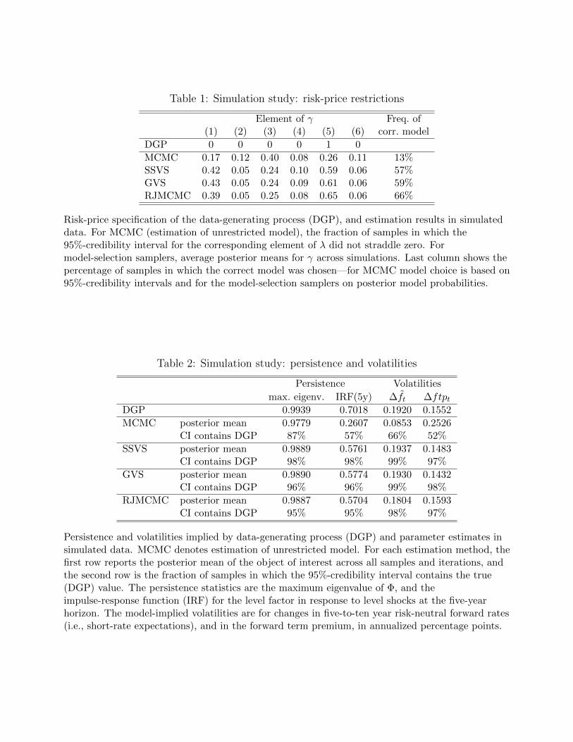
Table 1: Simulation study: risk-price restrictions

Element of γ Freq. of(1) (2) (3) (4) (5) (6) corr. model

DGP 0 0 0 0 1 0

MCMC 0.17 0.12 0.40 0.08 0.26 0.11 13%SSVS 0.42 0.05 0.24 0.10 0.59 0.06 57%GVS 0.43 0.05 0.24 0.09 0.61 0.06 59%RJMCMC 0.39 0.05 0.25 0.08 0.65 0.06 66%

Risk-price specification of the data-generating process (DGP), and estimation results in simulateddata. For MCMC (estimation of unrestricted model), the fraction of samples in which the95%-credibility interval for the corresponding element of λ did not straddle zero. Formodel-selection samplers, average posterior means for γ across simulations. Last column shows thepercentage of samples in which the correct model was chosen—for MCMC model choice is based on95%-credibility intervals and for the model-selection samplers on posterior model probabilities.

Table 2: Simulation study: persistence and volatilities

Persistence Volatilities

max. eigenv. IRF(5y) ∆ft ∆ftptDGP 0.9939 0.7018 0.1920 0.1552

MCMC posterior mean 0.9779 0.2607 0.0853 0.2526CI contains DGP 87% 57% 66% 52%

SSVS posterior mean 0.9889 0.5761 0.1937 0.1483CI contains DGP 98% 98% 99% 97%

GVS posterior mean 0.9890 0.5774 0.1930 0.1432CI contains DGP 96% 96% 99% 98%

RJMCMC posterior mean 0.9887 0.5704 0.1804 0.1593CI contains DGP 95% 95% 98% 97%

Persistence and volatilities implied by data-generating process (DGP) and parameter estimates insimulated data. MCMC denotes estimation of unrestricted model. For each estimation method, thefirst row reports the posterior mean of the object of interest across all samples and iterations, andthe second row is the fraction of samples in which the 95%-credibility interval contains the true(DGP) value. The persistence statistics are the maximum eigenvalue of Φ, and theimpulse-response function (IRF) for the level factor in response to level shocks at the five-yearhorizon. The model-implied volatilities are for changes in five-to-ten year risk-neutral forward rates(i.e., short-rate expectations), and in the forward term premium, in annualized percentage points.

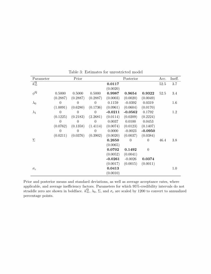
Table 3: Estimates for unrestricted model

Parameter Prior Posterior Acc. Ineff.

kQ∞ 0.0117 52.5 3.7(0.0020)

φQ 0.5000 0.5000 0.5000 0.9987 0.9654 0.9322 52.5 3.4(0.2887) (0.2887) (0.2887) (0.0003) (0.0020) (0.0049)

λ0 0 0 0 0.1159 -0.0392 0.0319 1.6(1.0091) (0.6280) (0.1736) (0.0961) (0.0604) (0.0170)

λ1 0 0 0 -0.0211 -0.0562 0.1792 1.2(0.1225) (0.2183) (2.2681) (0.0114) (0.0209) (0.2224)

0 0 0 0.0037 0.0100 0.0453(0.0762) (0.1358) (1.4114) (0.0074) (0.0123) (0.1407)

0 0 0 0.0000 -0.0023 -0.0950(0.0211) (0.0376) (0.3902) (0.0020) (0.0037) (0.0384)

Σ 0.2650 0 0 46.4 3.8(0.0065)0.0702 0.1492 0(0.0052) (0.0041)-0.0261 -0.0026 0.0374(0.0017) (0.0015) (0.0011)

σe 0.0413 1.0(0.0010)

Prior and posterior means and standard deviations, as well as average acceptance rates, whereapplicable, and average inefficiency factors. Parameters for which 95%-credibility intervals do notstraddle zero are shown in boldface. kQ∞, λ0, Σ, and σe are scaled by 1200 to convert to annualizedpercentage points.

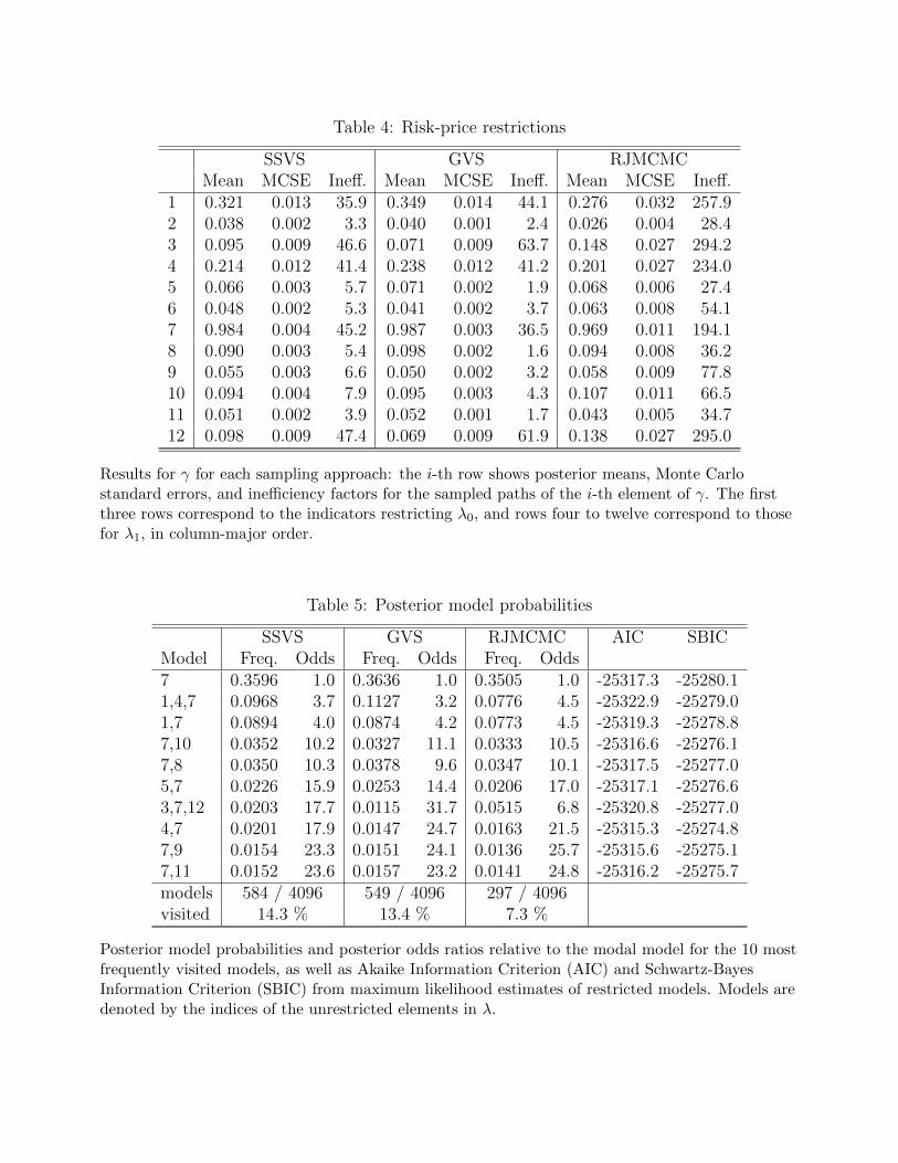
Table 4: Risk-price restrictions

SSVS GVS RJMCMCMean MCSE Ineff. Mean MCSE Ineff. Mean MCSE Ineff.

1 0.321 0.013 35.9 0.349 0.014 44.1 0.276 0.032 257.92 0.038 0.002 3.3 0.040 0.001 2.4 0.026 0.004 28.43 0.095 0.009 46.6 0.071 0.009 63.7 0.148 0.027 294.24 0.214 0.012 41.4 0.238 0.012 41.2 0.201 0.027 234.05 0.066 0.003 5.7 0.071 0.002 1.9 0.068 0.006 27.46 0.048 0.002 5.3 0.041 0.002 3.7 0.063 0.008 54.17 0.984 0.004 45.2 0.987 0.003 36.5 0.969 0.011 194.18 0.090 0.003 5.4 0.098 0.002 1.6 0.094 0.008 36.29 0.055 0.003 6.6 0.050 0.002 3.2 0.058 0.009 77.810 0.094 0.004 7.9 0.095 0.003 4.3 0.107 0.011 66.511 0.051 0.002 3.9 0.052 0.001 1.7 0.043 0.005 34.712 0.098 0.009 47.4 0.069 0.009 61.9 0.138 0.027 295.0

Results for γ for each sampling approach: the i-th row shows posterior means, Monte Carlostandard errors, and inefficiency factors for the sampled paths of the i-th element of γ. The firstthree rows correspond to the indicators restricting λ0, and rows four to twelve correspond to thosefor λ1, in column-major order.

Table 5: Posterior model probabilities

SSVS GVS RJMCMC AIC SBICModel Freq. Odds Freq. Odds Freq. Odds7 0.3596 1.0 0.3636 1.0 0.3505 1.0 -25317.3 -25280.11,4,7 0.0968 3.7 0.1127 3.2 0.0776 4.5 -25322.9 -25279.01,7 0.0894 4.0 0.0874 4.2 0.0773 4.5 -25319.3 -25278.87,10 0.0352 10.2 0.0327 11.1 0.0333 10.5 -25316.6 -25276.17,8 0.0350 10.3 0.0378 9.6 0.0347 10.1 -25317.5 -25277.05,7 0.0226 15.9 0.0253 14.4 0.0206 17.0 -25317.1 -25276.63,7,12 0.0203 17.7 0.0115 31.7 0.0515 6.8 -25320.8 -25277.04,7 0.0201 17.9 0.0147 24.7 0.0163 21.5 -25315.3 -25274.87,9 0.0154 23.3 0.0151 24.1 0.0136 25.7 -25315.6 -25275.17,11 0.0152 23.6 0.0157 23.2 0.0141 24.8 -25316.2 -25275.7models 584 / 4096 549 / 4096 297 / 4096visited 14.3 % 13.4 % 7.3 %

Posterior model probabilities and posterior odds ratios relative to the modal model for the 10 mostfrequently visited models, as well as Akaike Information Criterion (AIC) and Schwartz-BayesInformation Criterion (SBIC) from maximum likelihood estimates of restricted models. Models aredenoted by the indices of the unrestricted elements in λ.

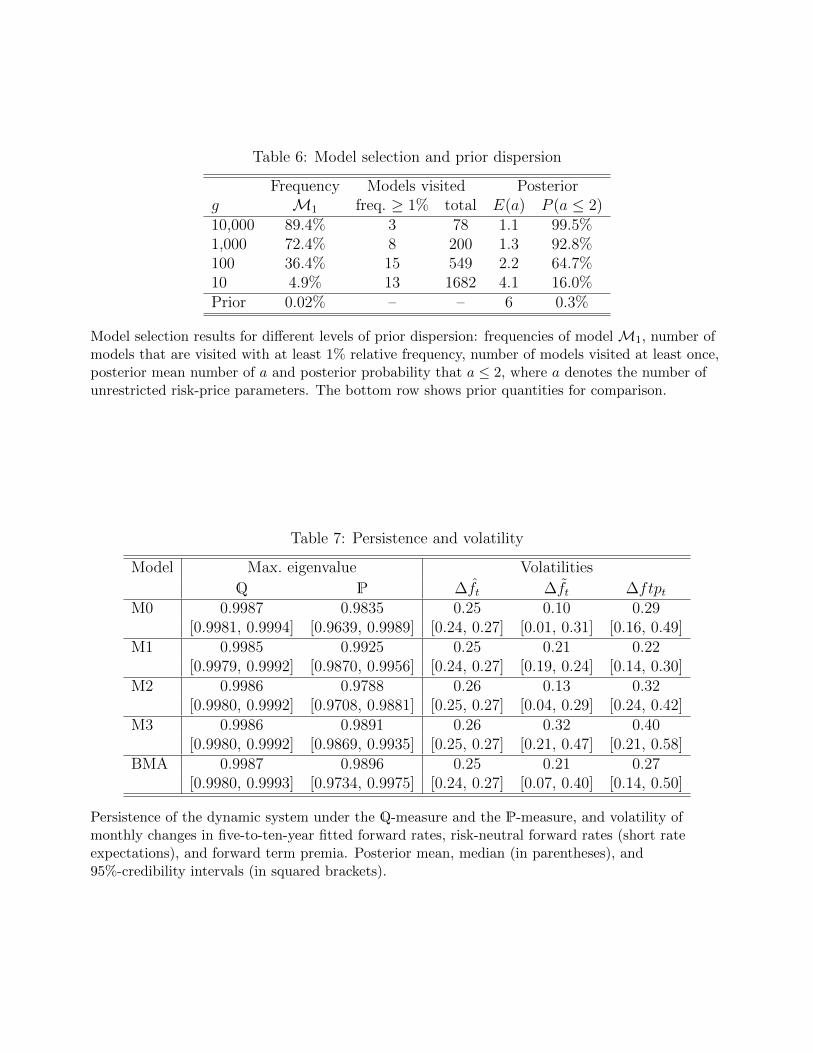
Table 6: Model selection and prior dispersion

Frequency Models visited Posteriorg M1 freq. ≥ 1% total E(a) P (a ≤ 2)10,000 89.4% 3 78 1.1 99.5%1,000 72.4% 8 200 1.3 92.8%100 36.4% 15 549 2.2 64.7%10 4.9% 13 1682 4.1 16.0%Prior 0.02% – – 6 0.3%

Model selection results for different levels of prior dispersion: frequencies of model M1, number ofmodels that are visited with at least 1% relative frequency, number of models visited at least once,posterior mean number of a and posterior probability that a ≤ 2, where a denotes the number ofunrestricted risk-price parameters. The bottom row shows prior quantities for comparison.

Table 7: Persistence and volatility

Model Max. eigenvalue Volatilities

Q P ∆ft ∆ft ∆ftptM0 0.9987 0.9835 0.25 0.10 0.29

[0.9981, 0.9994] [0.9639, 0.9989] [0.24, 0.27] [0.01, 0.31] [0.16, 0.49]M1 0.9985 0.9925 0.25 0.21 0.22

[0.9979, 0.9992] [0.9870, 0.9956] [0.24, 0.27] [0.19, 0.24] [0.14, 0.30]M2 0.9986 0.9788 0.26 0.13 0.32

[0.9980, 0.9992] [0.9708, 0.9881] [0.25, 0.27] [0.04, 0.29] [0.24, 0.42]M3 0.9986 0.9891 0.26 0.32 0.40

[0.9980, 0.9992] [0.9869, 0.9935] [0.25, 0.27] [0.21, 0.47] [0.21, 0.58]BMA 0.9987 0.9896 0.25 0.21 0.27

[0.9980, 0.9993] [0.9734, 0.9975] [0.24, 0.27] [0.07, 0.40] [0.14, 0.50]

Persistence of the dynamic system under the Q-measure and the P-measure, and volatility ofmonthly changes in five-to-ten-year fitted forward rates, risk-neutral forward rates (short rateexpectations), and forward term premia. Posterior mean, median (in parentheses), and95%-credibility intervals (in squared brackets).

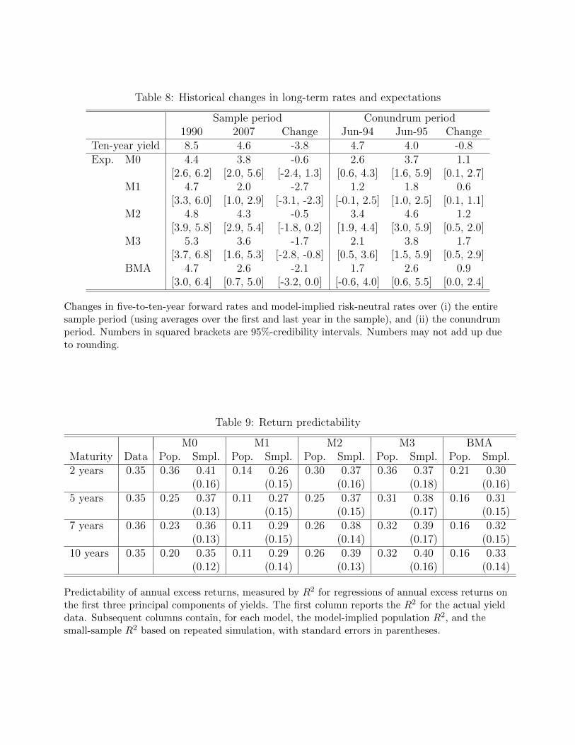
Table 8: Historical changes in long-term rates and expectations

Sample period Conundrum period1990 2007 Change Jun-94 Jun-95 Change

Ten-year yield 8.5 4.6 -3.8 4.7 4.0 -0.8Exp. M0 4.4 3.8 -0.6 2.6 3.7 1.1

[2.6, 6.2] [2.0, 5.6] [-2.4, 1.3] [0.6, 4.3] [1.6, 5.9] [0.1, 2.7]M1 4.7 2.0 -2.7 1.2 1.8 0.6

[3.3, 6.0] [1.0, 2.9] [-3.1, -2.3] [-0.1, 2.5] [1.0, 2.5] [0.1, 1.1]M2 4.8 4.3 -0.5 3.4 4.6 1.2

[3.9, 5.8] [2.9, 5.4] [-1.8, 0.2] [1.9, 4.4] [3.0, 5.9] [0.5, 2.0]M3 5.3 3.6 -1.7 2.1 3.8 1.7

[3.7, 6.8] [1.6, 5.3] [-2.8, -0.8] [0.5, 3.6] [1.5, 5.9] [0.5, 2.9]BMA 4.7 2.6 -2.1 1.7 2.6 0.9

[3.0, 6.4] [0.7, 5.0] [-3.2, 0.0] [-0.6, 4.0] [0.6, 5.5] [0.0, 2.4]

Changes in five-to-ten-year forward rates and model-implied risk-neutral rates over (i) the entiresample period (using averages over the first and last year in the sample), and (ii) the conundrumperiod. Numbers in squared brackets are 95%-credibility intervals. Numbers may not add up dueto rounding.

Table 9: Return predictability

M0 M1 M2 M3 BMAMaturity Data Pop. Smpl. Pop. Smpl. Pop. Smpl. Pop. Smpl. Pop. Smpl.2 years 0.35 0.36 0.41 0.14 0.26 0.30 0.37 0.36 0.37 0.21 0.30

(0.16) (0.15) (0.16) (0.18) (0.16)5 years 0.35 0.25 0.37 0.11 0.27 0.25 0.37 0.31 0.38 0.16 0.31

(0.13) (0.15) (0.15) (0.17) (0.15)7 years 0.36 0.23 0.36 0.11 0.29 0.26 0.38 0.32 0.39 0.16 0.32

(0.13) (0.15) (0.14) (0.17) (0.15)10 years 0.35 0.20 0.35 0.11 0.29 0.26 0.39 0.32 0.40 0.16 0.33

(0.12) (0.14) (0.13) (0.16) (0.14)

Predictability of annual excess returns, measured by R2 for regressions of annual excess returns onthe first three principal components of yields. The first column reports the R2 for the actual yielddata. Subsequent columns contain, for each model, the model-implied population R2, and thesmall-sample R2 based on repeated simulation, with standard errors in parentheses.

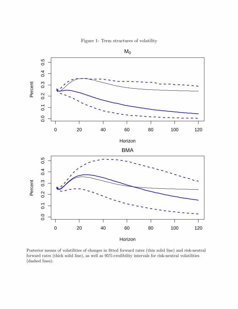
Figure 1: Term structures of volatility

0 20 40 60 80 100 120

0.0

0.1

0.2

0.3

0.4

0.5

Horizon

Per

cent

M0

0 20 40 60 80 100 120

0.0

0.1

0.2

0.3

0.4

0.5

Horizon

Per

cent

BMA

Posterior means of volatilities of changes in fitted forward rates (thin solid line) and risk-neutralforward rates (thick solid line), as well as 95%-credibility intervals for risk-neutral volatilities(dashed lines).

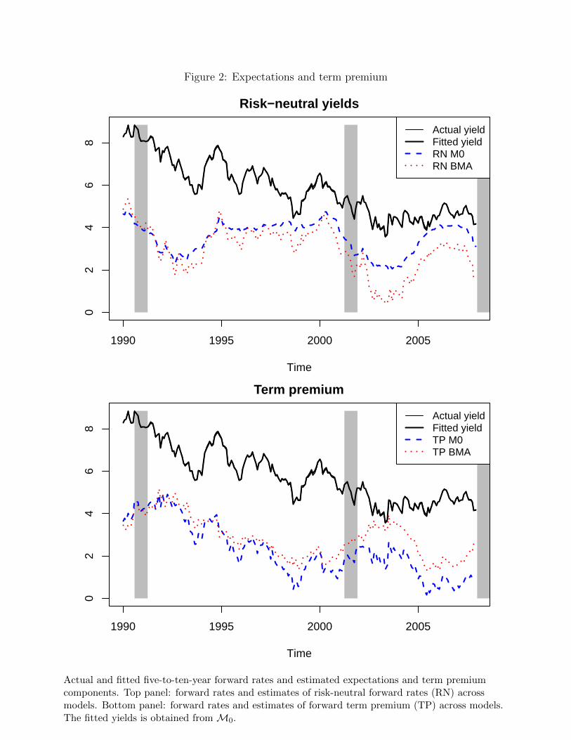
Figure 2: Expectations and term premium

Time

Per

cent

1990 1995 2000 2005

02

46

8

Actual yieldFitted yieldRN M0RN BMA

Risk−neutral yields

Time

Per

cent

1990 1995 2000 2005

02

46

8

Actual yieldFitted yieldTP M0TP BMA

Term premium

Actual and fitted five-to-ten-year forward rates and estimated expectations and term premiumcomponents. Top panel: forward rates and estimates of risk-neutral forward rates (RN) acrossmodels. Bottom panel: forward rates and estimates of forward term premium (TP) across models.The fitted yields is obtained from M0.