Embed Size (px)
Citation preview

Restoration of Bayer-Sampled Image Sequences
Murat Gevrekci‡, Bahadir K. Gunturk‡, and Yucel Altunbasak§
‡Department of Electrical and Computer Engineering
Louisiana State University
Baton Rouge, LA, 70803
Email: {lgevre1,bahadir}@ece.lsu.edu
§Department of Electrical and Computer Engineering
Georgia Institute of Technology
Atlanta, GA, 30332
Email: [email protected]
Abstract
Spatial resolution of digital images are limited due to optical/sensor blurring and sensor site density. In single-chip
digital cameras, the resolution is further degraded because such devices use a color filter array to capture only one
spectral component at a pixel location. The process of estimating the missing two color values at each pixel location
is known as demosaicking. Demosaicking methods usually exploit the correlation among color channels. When there
are multiple images, it is possible not only to have better estimates of the missing color values but also to improve
the spatial resolution further (using super-resolution reconstruction). In this paper, we propose a multi-frame spatial
resolution enhancement algorithm based on the projections onto convex sets (POCS) technique.
2
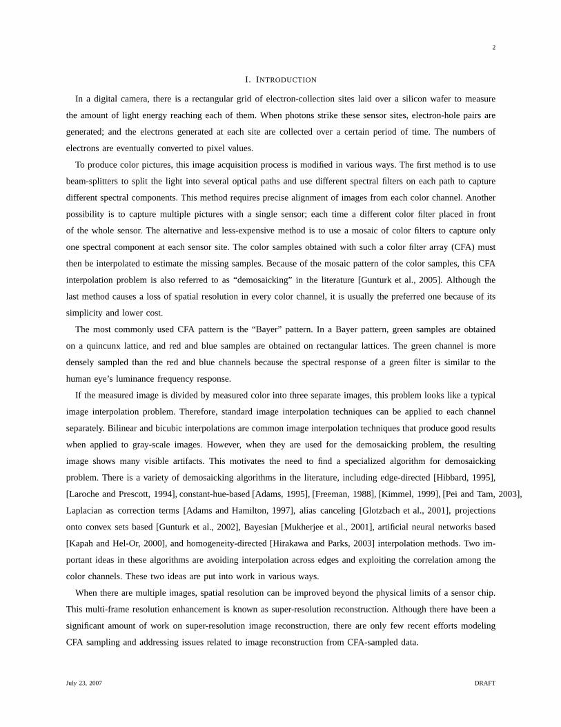
I. I NTRODUCTION
In a digital camera, there is a rectangular grid of electron-collection sites laid over a silicon wafer to measure
the amount of light energy reaching each of them. When photons strike these sensor sites, electron-hole pairs are
generated; and the electrons generated at each site are collected over a certain period of time. The numbers of
electrons are eventually converted to pixel values.
To produce color pictures, this image acquisition process is modified in various ways. The first method is to use
beam-splitters to split the light into several optical paths and use different spectral filters on each path to capture
different spectral components. This method requires precise alignment of images from each color channel. Another
possibility is to capture multiple pictures with a single sensor; each time a different color filter placed in front
of the whole sensor. The alternative and less-expensive method is to use a mosaic of color filters to capture only
one spectral component at each sensor site. The color samples obtained with such a color filter array (CFA) must
then be interpolated to estimate the missing samples. Because of the mosaic pattern of the color samples, this CFA
interpolation problem is also referred to as “demosaicking” in the literature [Gunturk et al., 2005]. Although the
last method causes a loss of spatial resolution in every color channel, it is usually the preferred one because of its
simplicity and lower cost.
The most commonly used CFA pattern is the “Bayer” pattern. In a Bayer pattern, green samples are obtained
on a quincunx lattice, and red and blue samples are obtained on rectangular lattices. The green channel is more
densely sampled than the red and blue channels because the spectral response of a green filter is similar to the
human eye’s luminance frequency response.
If the measured image is divided by measured color into three separate images, this problem looks like a typical
image interpolation problem. Therefore, standard image interpolation techniques can be applied to each channel
separately. Bilinear and bicubic interpolations are common image interpolation techniques that produce good results
when applied to gray-scale images. However, when they are used for the demosaicking problem, the resulting
image shows many visible artifacts. This motivates the need to find a specialized algorithm for demosaicking
problem. There is a variety of demosaicking algorithms in the literature, including edge-directed [Hibbard, 1995],
[Laroche and Prescott, 1994], constant-hue-based [Adams, 1995], [Freeman, 1988], [Kimmel, 1999], [Pei and Tam, 2003],
Laplacian as correction terms [Adams and Hamilton, 1997], alias canceling [Glotzbach et al., 2001], projections
onto convex sets based [Gunturk et al., 2002], Bayesian [Mukherjee et al., 2001], artificial neural networks based
[Kapah and Hel-Or, 2000], and homogeneity-directed [Hirakawa and Parks, 2003] interpolation methods. Two im-
portant ideas in these algorithms are avoiding interpolation across edges and exploiting the correlation among the
color channels. These two ideas are put into work in various ways.
When there are multiple images, spatial resolution can be improved beyond the physical limits of a sensor chip.
This multi-frame resolution enhancement is known as super-resolution reconstruction. Although there have been a
significant amount of work on super-resolution image reconstruction, there are only few recent efforts modeling
CFA sampling and addressing issues related to image reconstruction from CFA-sampled data.
July 23, 2007 DRAFT
3
In [Farsiu et al., 2006], data fidelity and regularization terms are combined to produce high-resolution images.
The data fidelity term is based on a cost function that consists of the the sum of residual differences between
actual observations and high-resolution image projected onto observations (simulated observations). Regularization
functions are added to this cost function to eliminate color artifacts and preserve edge structures. These additional
constraints are defined as luminance, chrominance, and orientation regularization in [Farsiu et al., 2006]. A similar
algorithm is presented in [Gotoh and Okutomi, 2004].
Among different demosaicking approaches, the POCS-based demosaicking algorithm has one of the best perfor-
mance [Gunturk et al., 2002], [Gunturk et al., 2005]. One advantage of the POCS framework is that new constraints
can be easily incorporated into a POCS-based algorithm. Here, we present POCS-based algorithms for multi-frame
resolution enhancement of Bayer CFA sampled images. We investigate two approaches:demosaicking and super-
resolution(DSR) andonly super-resolution(OSR). In DSR approach, we separate the restoration process into two
parts. The first part is multi-frame demosaicking, where missing color samples are estimated. The second part is
super-resolution reconstruction, where sub-pixel level resolution is achieved. In OSR approach, super-resolution
image is reconstructed without demosaicking, using Bayer pattern masks only for computing the residual of each
color channel.
In Section II, we present an imaging model that includes CFA sampling. We introduce our POCS-based multi-
frame demosaicking algorithm in Section III. This Section includes three constraint sets and corresponding projection
operators for multi-frame demosaicking. In Section IV, we explain how to achieve sub-pixel resolution. Experimental
results and discussions are provided in Section V.
II. I MAGING MODEL
We use an image acquisition model that includes CFA sampling in addition to motion and blurring. The model
has two steps: the first step models conversion of a high-resolution full-color image into a low-resolution full-color
image. The second step models color filter sampling of full-color low-resolution image.
Let xS a color channel of a high-resolution image, where a channel can be red (xR), green (xG), and blue
(xB). The ith observation,y(i)S , is obtained from this high-resolution image through spatial warping, blurring, and
downsampling operations:
y(i)S = DCW (i)xS , for S = R, G,B, and i = 1, 2, ..., K, (1)
whereK is the number of input images,W (i) is the warping operation (to account for the relative motion between
observations),C is the convolution operation (to account for the point spread function of the camera), andD is
the downsampling operation (to account for the spatial sampling of the sensor).
The full-color image (y(i)R ,y(i)
G ,y(i)B ) is then converted to a mosaicked observationz(i) according to a CFA
sampling pattern:
z(i) =∑
S=R,G,B
MSy(i)S (2)
July 23, 2007 DRAFT
4
whereMS takes only one of the color samples at a pixel according to the pattern. For example, at red pixel location,
[MR, MG, MB ] is [1, 0, 0].
We investigate two approaches to obtainxS . In DSR approach, each full-color low-resolution imagey(i)S is
estimated from the multiple observationsz(i), and then super-resolution reconstruction is applied to these estimates
y(i)S to obtainxS . In the OSR approach,xS is obtained directly fromz(i) without estimatingy(i)
S .
III. M ULTI -FRAME DEMOSAICKING
In this section, we introduce multi-frame demosaicking, where multiple images are used to estimate missing
samples in a Bayer-sampled color image. The process is based on the POCS technique, where an initial estimate
is projected onto convex constraint sets iteratively to reach a solution that is consistent with all constraints about
the solution [Combettes, 1993].
This algorithm is based on the demosaicking approach presented in [Gunturk et al., 2002]. In [Gunturk et al., 2002],
we define two constraint sets. The first constraint set stems from inter-channel correlation. It is based on the idea
that high-frequency components of red, green, and blue channels should be similar in an image. This turns out to
be a very effective constraint set. This constraint set is also used in this paper.
The second constraint set ensures that the reconstructed image is consistent with the observed data of the same
image. This constraint set can be improved when there are multiple observations of the same scene. A missing
sample (due to the CFA sampling) in an image could have been captured in another image due to the relative motion
between observations. It is possible to obtain a better estimate of a missing sample by taking multiple images into
account. Therefore, we define a constraint set based on samples coming from multiple images.
In addition to previous constraint sets, we propose a third constraint set in this paper to achieve color consistency.
Consistent neighbors of a pixel are determined according to both spatial and intensity closeness. Intensity of a pixel
is updated using the weighted average value of its consistent neighbors. These constraint sets are examined in
following sections.
A. Detail Constraint Set
Let Wk be an operator that produces thekth subband of an image. There are four frequency subbands(k =
LL,LH, HL,HH) corresponding to low-pass filtering and high-pass filtering permutations along horizontal and
vertical dimensions. (A brief review of the subband decomposition is provided in the appendix.)
The “detail” constraint set (Cd) forces the details (high-frequency components) of the red and blue channels to
be similar to the details of the green channel at every pixel location(n1, n2), and is defined as follows:
Cd =
y(i)S (n1, n2) :
∣∣∣(Wky
(i)S
)(n1, n2)−
(Wky
(i)G
)(n1, n2)
∣∣∣ ≤ Td(n1, n2)
∀ (n1, n2), for k = LH, HL, HH and S = R,B
, (3)
whereTd(n1, n2) is a positive threshold that quantifies the “closeness” of the detail subbands to each other. For
details and further discussion on this constraint set, we refer the reader to [Gunturk et al., 2002].
July 23, 2007 DRAFT
5
II
I
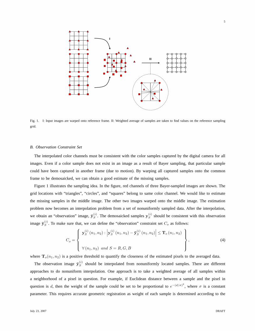
Fig. 1. I: Input images are warped onto reference frame. II: Weighted average of samples are taken to find values on the reference sampling
grid.
B. Observation Constraint Set
The interpolated color channels must be consistent with the color samples captured by the digital camera for all
images. Even if a color sample does not exist in an image as a result of Bayer sampling, that particular sample
could have been captured in another frame (due to motion). By warping all captured samples onto the common
frame to be demosaicked, we can obtain a good estimate of the missing samples.
Figure 1 illustrates the sampling idea. In the figure, red channels of three Bayer-sampled images are shown. The
grid locations with “triangles”, “circles”, and “squares” belong to same color channel. We would like to estimate
the missing samples in the middle image. The other two images warped onto the middle image. The estimation
problem now becomes an interpolation problem from a set of nonuniformly sampled data. After the interpolation,
we obtain an “observation” image,y(i)S . The demosaicked samplesy(i)
S should be consistent with this observation
imagey(i)S . To make sure that, we can define the “observation” constraint setCo as follows:
Co =
y(i)S (n1, n2) :
∣∣∣y(i)S (n1, n2)− y(i)
S (n1, n2)∣∣∣ ≤ To (n1, n2)
∀ (n1, n2) and S = R, G, B
, (4)
whereTo(n1, n2) is a positive threshold to quantify the closeness of the estimated pixels to the averaged data.
The observation imagey(i)S should be interpolated from nonuniformly located samples. There are different
approaches to do nonuniform interpolation. One approach is to take a weighted average of all samples within
a neighborhood of a pixel in question. For example, if Euclidean distance between a sample and the pixel in
question isd, then the weight of the sample could be set to be proportional toe−(d/σ)2 , whereσ is a constant
parameter. This requires accurate geometric registration as weight of each sample is determined according to the
July 23, 2007 DRAFT
6
spatial closeness to the sampling location. In our experiments, we used simple bilinear interpolation to estimate the
missing samples. That is, all frames are warped onto the reference frame using bilinear interpolation. These warped
images are then averaged to obtainy(i)S .
One benefit of using this constraint set is noise reduction. When the input data is noisy, constraining the solution
to be close to the observation imagey(i)S prevents amplification of noise and color artifacts.
C. Color Consistency Constraint Set
The third constraint set is the color consistency constraint set. It is reasonable to expect pixels with similar
green intensities to have similar red and blue intensities within a small spatial neighborhood. Therefore, we define
spatio-intensity neighborhoodof a pixel. Suppose that green channelxG of an image is already interpolated and
we would like to estimate the red value at a particular pixel(n1, n2). Then, the spatio-intensity neighborhood of
the pixel (n1, n2) is defined as
N (n1, n2) ={
(m1,m2) : ‖(m1, m2)− (n1, n2)‖ ≤ τS and∣∣∣y(i)
G (m1,m2)− y(i)G (n1, n2)
∣∣∣ ≤ τI
}, (5)
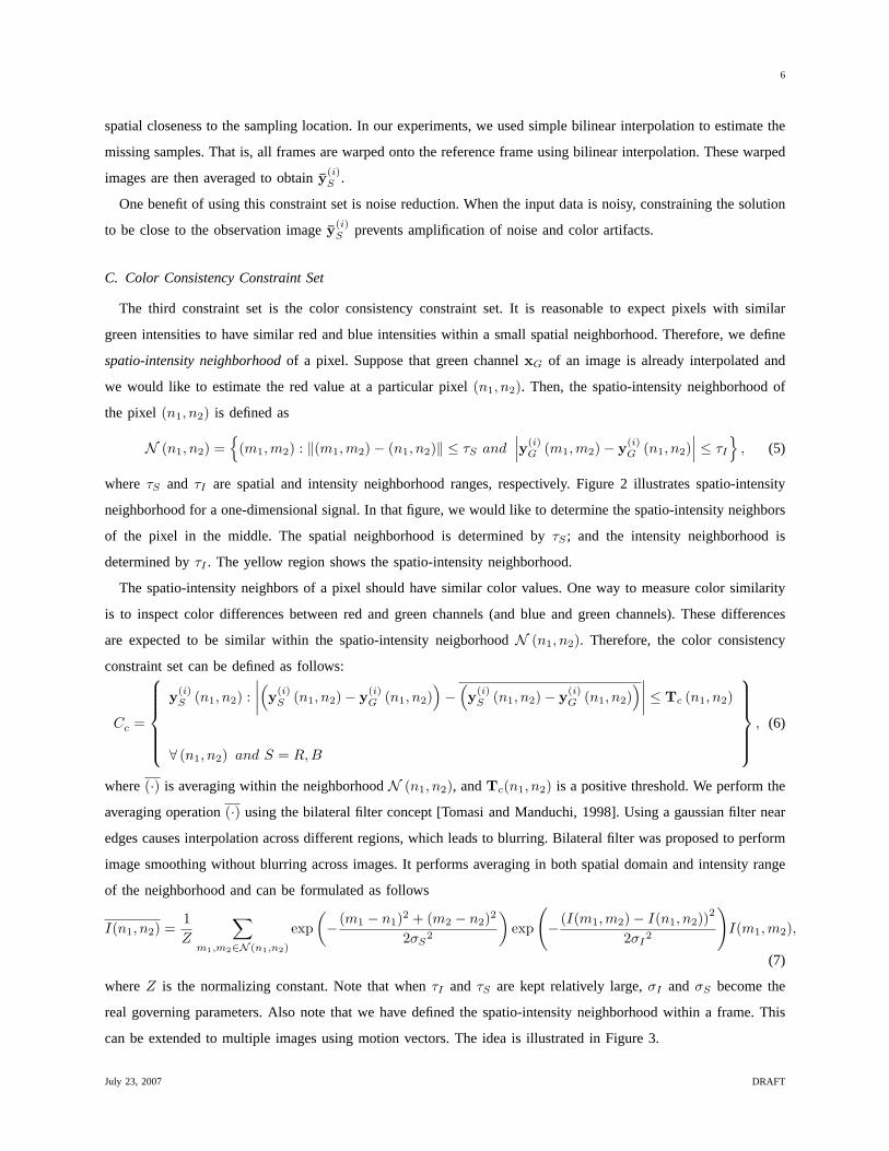
where τS and τI are spatial and intensity neighborhood ranges, respectively. Figure 2 illustrates spatio-intensity
neighborhood for a one-dimensional signal. In that figure, we would like to determine the spatio-intensity neighbors
of the pixel in the middle. The spatial neighborhood is determined byτS ; and the intensity neighborhood is
determined byτI . The yellow region shows the spatio-intensity neighborhood.
The spatio-intensity neighbors of a pixel should have similar color values. One way to measure color similarity
is to inspect color differences between red and green channels (and blue and green channels). These differences
are expected to be similar within the spatio-intensity neigborhoodN (n1, n2). Therefore, the color consistency
constraint set can be defined as follows:
Cc =
y(i)S (n1, n2) :
∣∣∣∣(y(i)
S (n1, n2)− y(i)G (n1, n2)
)−
(y(i)
S (n1, n2)− y(i)G (n1, n2)
)∣∣∣∣ ≤ Tc (n1, n2)
∀ (n1, n2) and S = R,B
, (6)
where(·) is averaging within the neighborhoodN (n1, n2), andTc(n1, n2) is a positive threshold. We perform the
averaging operation(·) using the bilateral filter concept [Tomasi and Manduchi, 1998]. Using a gaussian filter near
edges causes interpolation across different regions, which leads to blurring. Bilateral filter was proposed to perform
image smoothing without blurring across images. It performs averaging in both spatial domain and intensity range
of the neighborhood and can be formulated as follows
I(n1, n2) =1Z
∑
m1,m2∈N (n1,n2)
exp(− (m1 − n1)2 + (m2 − n2)2
2σS2
)exp
(− (I(m1,m2)− I(n1, n2))
2
2σI2
)I(m1,m2),
(7)
whereZ is the normalizing constant. Note that whenτI and τS are kept relatively large,σI and σS become the
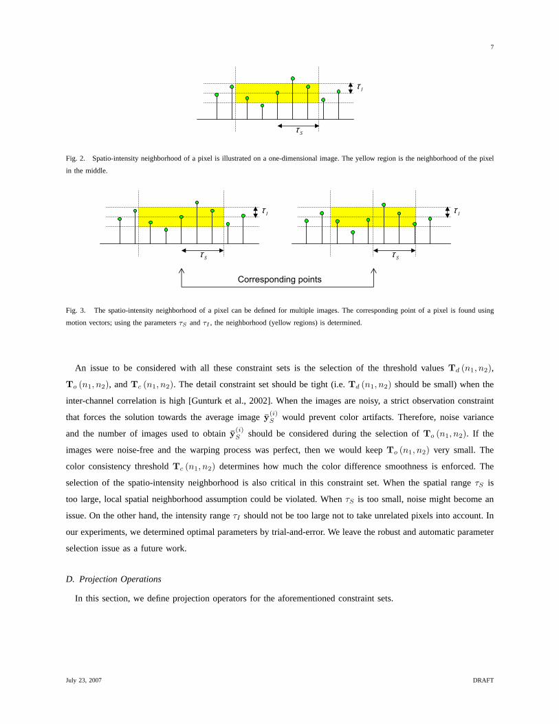
real governing parameters. Also note that we have defined the spatio-intensity neighborhood within a frame. This
can be extended to multiple images using motion vectors. The idea is illustrated in Figure 3.
July 23, 2007 DRAFT
7
Sτ
Iτ
Fig. 2. Spatio-intensity neighborhood of a pixel is illustrated on a one-dimensional image. The yellow region is the neighborhood of the pixel
in the middle.
Sτ
Iτ
Sτ
Iτ
Corresponding points
Fig. 3. The spatio-intensity neighborhood of a pixel can be defined for multiple images. The corresponding point of a pixel is found using
motion vectors; using the parametersτS andτI , the neighborhood (yellow regions) is determined.
An issue to be considered with all these constraint sets is the selection of the threshold valuesTd (n1, n2),
To (n1, n2), andTc (n1, n2). The detail constraint set should be tight (i.e.Td (n1, n2) should be small) when the
inter-channel correlation is high [Gunturk et al., 2002]. When the images are noisy, a strict observation constraint
that forces the solution towards the average imagey(i)S would prevent color artifacts. Therefore, noise variance
and the number of images used to obtainy(i)S should be considered during the selection ofTo (n1, n2). If the
images were noise-free and the warping process was perfect, then we would keepTo (n1, n2) very small. The
color consistency thresholdTc (n1, n2) determines how much the color difference smoothness is enforced. The
selection of the spatio-intensity neighborhood is also critical in this constraint set. When the spatial rangeτS is
too large, local spatial neighborhood assumption could be violated. WhenτS is too small, noise might become an
issue. On the other hand, the intensity rangeτI should not be too large not to take unrelated pixels into account. In
our experiments, we determined optimal parameters by trial-and-error. We leave the robust and automatic parameter
selection issue as a future work.
D. Projection Operations
In this section, we define projection operators for the aforementioned constraint sets.
July 23, 2007 DRAFT
8
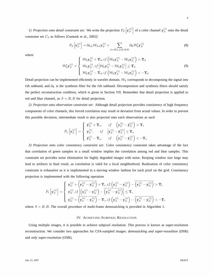
1) Projection onto detail constraint set:We write the projectionPd
[y(i)
S
]of a color channely(i)
S onto the detail
constraint setCd as follows [Gunturk et al., 2002]:
Pd
[y(i)
S
]= ULLWLLy(i)
S +∑
k=HL,LH,HH
UkW ′ky
(i)S (8)
where
W ′ky
(i)S =
Wky(i)G + Td, if
(Wky
(i)S −Wky
(i)G
)> Td
Wky(i)S , if
∣∣∣Wky(i)S −Wky
(i)G
∣∣∣ ≤ Td
Wky(i)G −Td, if
(Wky
(i)S −Wky
(i)G
)< −Td
(9)
Detail projection can be implemented efficiently in wavelet domain.Wk corresponds to decomposing the signal into
kth subband, andUk is the synthesis filter for thekth subband. Decomposition and synthesis filters should satisfy
the perfect reconstruction condition, which is given in Section VII. Remember that detail projection is applied to
red and blue channel, asS = R,B for detail projection.
2) Projection onto observation constraint set:Although detail projection provides consistency of high frequency
components of color channels, this forced correlation may result in deviation from actual values. In order to prevent
this possible deviation, intermediate result is also projected onto each observations as such
Po
[y(i)
S
]=
y(i)S + To, if
(y(i)
S − y(i)S
)> To
y(i)S , if
∣∣∣y(i)S − y(i)
S
∣∣∣ ≤ To
y(i)S −To, if
(y(i)
S − y(i)S
)< −To
3) Projection onto color consistency constraint set:Color consistency constraint takes advantage of the fact
that correlation of green samples in a small window implies the correlation among red and blue samples. This
constraint set provides noise elimination for highly degraded images with noise. Keeping window size large may
lead to artifacts in final result, as correlation is valid for a local neighborhood. Realization of color consistency
constraint is exhaustive as it is implemented in a moving window fashion for each pixel on the grid. Consistency
projection is implemented with the following operation
Pc
[y(i)
S
]=
y(i)G +
(y(i)
S − y(i)G
)+ Tc, if
(y(i)
S − y(i)G
)−
(y(i)
S − y(i)G
)> Tc
y(i)S , if
∣∣∣∣(y(i)
S − y(i)G
)−
(y(i)
S − y(i)G
)∣∣∣∣ ≤ Tc
y(i)G +
(y(i)
S − y(i)G
)−Tc, if
(y(i)
S − y(i)G
)−
(y(i)
S − y(i)G
)< −Tc
whereS = R, B. The overall procedure of multi-frame demosaicking is provided in Algorithm 1.
IV. A CHIEVING SUBPIXEL RESOLUTION
Using multiple images, it is possible to achieve subpixel resolution. This process is known as super-resolution
reconstruction. We consider two approaches for CFA-sampled images:demosaicking and super-resoultion(DSR)
andonly super-resolution(OSR).
July 23, 2007 DRAFT
9
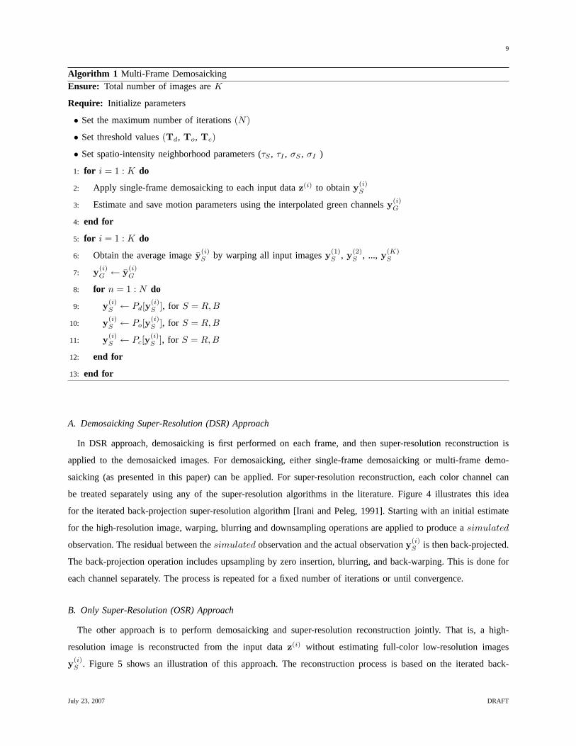
Algorithm 1 Multi-Frame DemosaickingEnsure: Total number of images areK
Require: Initialize parameters
• Set the maximum number of iterations(N)
• Set threshold values(Td, To, Tc)
• Set spatio-intensity neighborhood parameters (τS , τI , σS , σI )
1: for i = 1 : K do
2: Apply single-frame demosaicking to each input dataz(i) to obtainy(i)S
3: Estimate and save motion parameters using the interpolated green channelsy(i)G
4: end for
5: for i = 1 : K do
6: Obtain the average imagey(i)S by warping all input imagesy(1)
S , y(2)S , ..., y(K)
S
7: y(i)G ← y(i)
G
8: for n = 1 : N do
9: y(i)S ← Pd[y
(i)S ], for S = R,B
10: y(i)S ← Po[y
(i)S ], for S = R, B
11: y(i)S ← Pc[y
(i)S ], for S = R,B
12: end for
13: end for
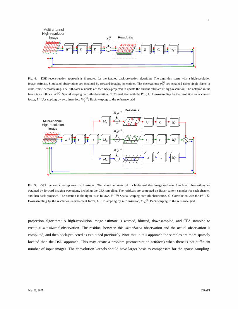
A. Demosaicking Super-Resolution (DSR) Approach
In DSR approach, demosaicking is first performed on each frame, and then super-resolution reconstruction is
applied to the demosaicked images. For demosaicking, either single-frame demosaicking or multi-frame demo-
saicking (as presented in this paper) can be applied. For super-resolution reconstruction, each color channel can
be treated separately using any of the super-resolution algorithms in the literature. Figure 4 illustrates this idea
for the iterated back-projection super-resolution algorithm [Irani and Peleg, 1991]. Starting with an initial estimate
for the high-resolution image, warping, blurring and downsampling operations are applied to produce asimulated
observation. The residual between thesimulated observation and the actual observationy(i)S is then back-projected.
The back-projection operation includes upsampling by zero insertion, blurring, and back-warping. This is done for
each channel separately. The process is repeated for a fixed number of iterations or until convergence.
B. Only Super-Resolution (OSR) Approach
The other approach is to perform demosaicking and super-resolution reconstruction jointly. That is, a high-
resolution image is reconstructed from the input dataz(i) without estimating full-color low-resolution images
y(i)S . Figure 5 shows an illustration of this approach. The reconstruction process is based on the iterated back-
July 23, 2007 DRAFT
10
)(iW C D
)(iSy
U C )(ibW
Residuals
R RR RR RR R
R RR R
Multi-channel High-resolution
Image
Fig. 4. DSR reconstruction approach is illustrated for the iterated back-projection algorithm. The algorithm starts with a high-resolution
image estimate. Simulated observations are obtained by forward imaging operations. The observationsy(i)S are obtained using single-frame or
multi-frame demosaicking. The full-color residuals are then back-projected to update the current estimate of high-resolution. The notation in the
figure is as follows.W (i): Spatial warping ontoith observation,C: Convolution with the PSF,D: Downsampling by the resolution enhancement
factor,U : Upsampling by zero insertion,W (i)b
: Back-warping to the reference grid.
R R
R R
G G
G GG G
B B
)(iW C D
RM
GM
BM
)(iR zM
)(iG zM
)(iB zM
U C
U C
U C
)(ibW
)(ibW
)(ibW
Residuals
Multi-channel High-resolution
Image
Fig. 5. OSR reconstruction approach is illustrated. The algorithm starts with a high-resolution image estimate. Simulated observations are
obtained by forward imaging operations, including the CFA sampling. The residuals are computed on Bayer pattern samples for each channel,
and then back-projected. The notation in the figure is as follows.W (i): Spatial warping ontoith observation,C: Convolution with the PSF,D:
Downsampling by the resolution enhancement factor,U : Upsampling by zero insertion,W (i)b
: Back-warping to the reference grid.
projection algorithm: A high-resolution image estimate is warped, blurred, downsampled, and CFA sampled to
create asimulated observation. The residual between thissimulated observation and the actual observation is
computed, and then back-projected as explained previously. Note that in this approach the samples are more sparsely
located than the DSR approach. This may create a problem (reconstruction artifacts) when there is not sufficient
number of input images. The convolution kernels should have larger basis to compensate for the sparse sampling.
July 23, 2007 DRAFT
11
(a) (b)
(c) (d)
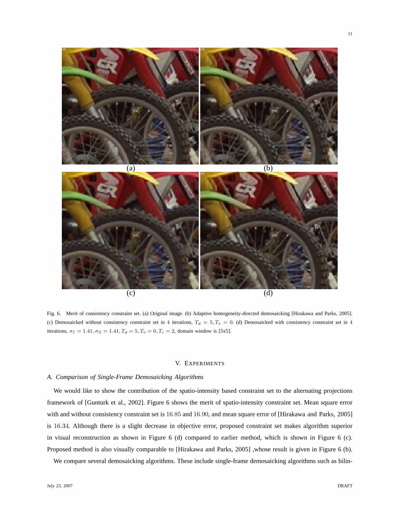
Fig. 6. Merit of consistency constraint set. (a) Original image. (b) Adaptive homogeneity-directed demosaicking [Hirakawa and Parks, 2005].
(c) Demosaicked without consistency constraint set in4 iterations,Td = 5, To = 0. (d) Demosaicked with consistency constraint set in4
iterations,σI = 1.41, σS = 1.41, Td = 5, To = 0, Tc = 2, domain window is [5x5].
V. EXPERIMENTS
A. Comparison of Single-Frame Demosaicking Algorithms
We would like to show the contribution of the spatio-intensity based constraint set to the alternating projections
framework of [Gunturk et al., 2002]. Figure 6 shows the merit of spatio-intensity constraint set. Mean square error
with and without consistency constraint set is16.85 and16.90, and mean square error of [Hirakawa and Parks, 2005]
is 16.34. Although there is a slight decrease in objective error, proposed constraint set makes algorithm superior
in visual reconstruction as shown in Figure 6 (d) compared to earlier method, which is shown in Figure 6 (c).
Proposed method is also visually comparable to [Hirakawa and Parks, 2005] ,whose result is given in Figure 6 (b).
We compare several demosaicking algorithms. These include single-frame demosaicking algorithms such as bilin-
July 23, 2007 DRAFT
12
ear interpolation, edge-directed interpolation [Laroche and Prescott, 1994], alternating projections [Gunturk et al., 2002]
and adaptive homogeneity directed demosaicking [Hirakawa and Parks, 2005] in comparison with our proposed
demosaicking algorithm. In this section proposed algorithm is applied using single image framework as existing
demosaicking algorithms are applied on single frame, and it is fair to make comparison on same basis. Multi-frame
demosaicking in conjunction with the resolution enhancement will be performed in next section.
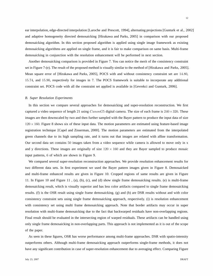
Another demosaicking comparison is provided in Figure 7. You can notice the merit of the consistency constraint
set in Figure 7-(e). The result of the proposed method is visually similar to the method of [Hirakawa and Parks, 2005].
Mean square error of [Hirakawa and Parks, 2005], POCS with and without consistency constraint set are14.80,
15.74, and 15.90, respectively for images in 7. The POCS framework is suitable to incorporate any additional
constraint set. POCS code with all the constraint set applied is available in [Gevrekci and Gunturk, 2006].
B. Super Resolution Experiments
In this section we compare several approaches for demosaicking and super-resolution reconstruction. We first
captured a video sequence of length 21 usingCanonG5 digital camera. The size of each frame is240×320. These
images are then downscaled by two and then further sampled with the Bayer pattern to produce the input data of size
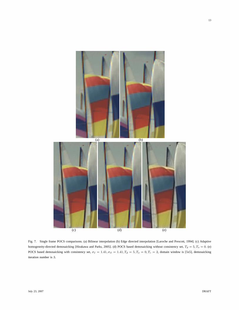
120× 160. Figure 8 shows six of these input data. The motion parameters are estimated using feature-based image
registration technique [Capel and Zisserman, 2000]. The motion parameters are estimated from the interpolated
green channels due to its high sampling rate, and it turns out that images are related with affine transformation.
Our second data set contains50 images taken from a video sequence while camera is allowed to move only in x
and y directions. These images are originally of size120 × 160 and they are Bayer sampled to produce mosaic
input patterns,6 of which are shown in Figure 9.
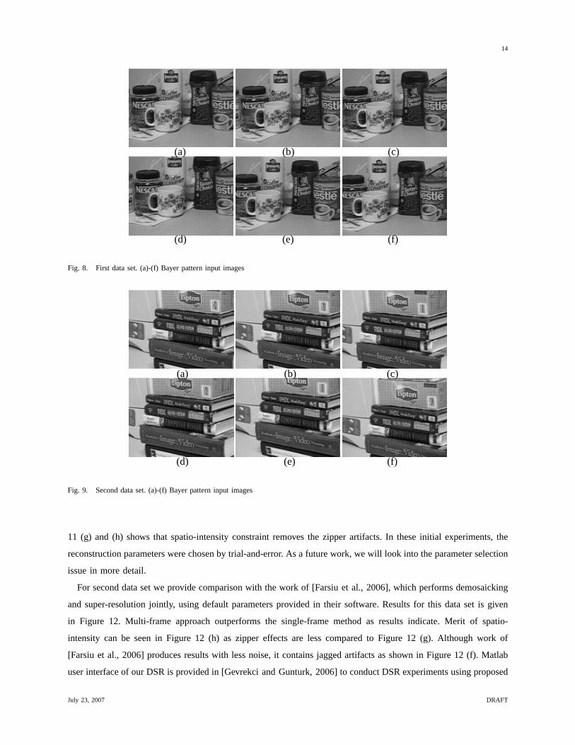
We compared several super-resolution reconstruction approaches. We provide resolution enhancement results for
two different data sets. In first experiment we used the Bayer pattern images given in Figure 8. Demosaicked
and multi-frame enhanced results are given in Figure 10. Cropped regions of same results are given in Figure
11. In Figure 10 and Figure 11 , (a), (b), (c), and (d) show single frame demosaicking results. (e) is multi-frame
demosaicking result, which is visually superior and has less color artifacts compared to single frame demosaicking
results. (f) is the OSR result using single frame demosaicking. (g) and (h) are DSR results without and with color
consistency constraint sets using single frame demosaicking approach, respectively. (i) is resolution enhancement
with consistency set using multi frame demosaicking approach. Note that border artifacts may occur in super
resolution with multi-frame demosaicking due to the fact that backwarped residuals have non-overlapping regions.
Final result should be evaluated in the intersecting region of warped residuals. These artifacts can be handled using
only single frame demosaicking in non-overlapping parts. This approach is not implemented as it is out of the scope
of the paper.
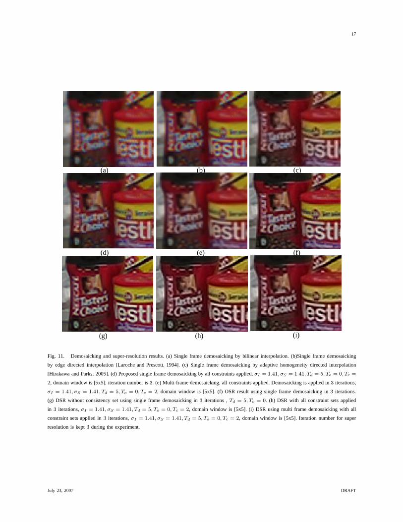
As seen in these figures, OSR has worse performance among multi-frame approaches. DSR with spatio-intensity
outperforms others. Although multi-frame demosaicking approach outperforms single-frame methods, it does not
have any significant contribution in case of super-resolution enhancement due to averaging effect. Comparing Figure
July 23, 2007 DRAFT
13
(a) (b)
(c) (d) (e)
Fig. 7. Single frame POCS comparisons. (a) Bilinear interpolation (b) Edge directed interpolation [Laroche and Prescott, 1994]. (c) Adaptive
homogeneity-directed demosaicking [Hirakawa and Parks, 2005]. (d) POCS based demosaicking without consistency set,Td = 5, To = 0. (e)
POCS based demosaicking with consistency set,σI = 1.41, σS = 1.41, Td = 5, To = 0, Tc = 2, domain window is [5x5], demosaicking
iteration number is3.
July 23, 2007 DRAFT
14
(a) (b) (c)
(d) (e) (f)
Fig. 8. First data set. (a)-(f) Bayer pattern input images
(a) (b) (c)
(d) (e) (f)
Fig. 9. Second data set. (a)-(f) Bayer pattern input images
11 (g) and (h) shows that spatio-intensity constraint removes the zipper artifacts. In these initial experiments, the
reconstruction parameters were chosen by trial-and-error. As a future work, we will look into the parameter selection
issue in more detail.
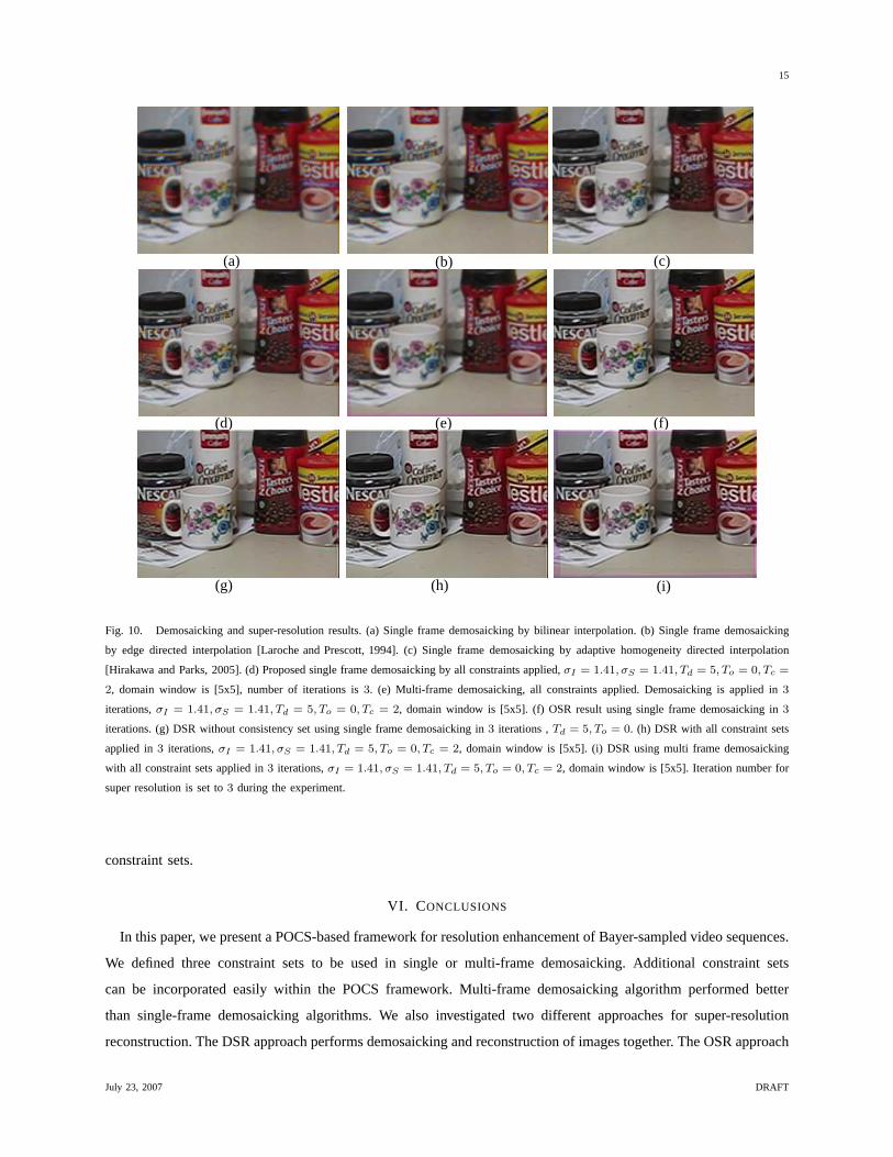
For second data set we provide comparison with the work of [Farsiu et al., 2006], which performs demosaicking
and super-resolution jointly, using default parameters provided in their software. Results for this data set is given
in Figure 12. Multi-frame approach outperforms the single-frame method as results indicate. Merit of spatio-
intensity can be seen in Figure 12 (h) as zipper effects are less compared to Figure 12 (g). Although work of
[Farsiu et al., 2006] produces results with less noise, it contains jagged artifacts as shown in Figure 12 (f). Matlab
user interface of our DSR is provided in [Gevrekci and Gunturk, 2006] to conduct DSR experiments using proposed
July 23, 2007 DRAFT
15
(a) (b) (c)
(d) (e) (f)
(g) (h) (i)
Fig. 10. Demosaicking and super-resolution results. (a) Single frame demosaicking by bilinear interpolation. (b) Single frame demosaicking
by edge directed interpolation [Laroche and Prescott, 1994]. (c) Single frame demosaicking by adaptive homogeneity directed interpolation
[Hirakawa and Parks, 2005]. (d) Proposed single frame demosaicking by all constraints applied,σI = 1.41, σS = 1.41, Td = 5, To = 0, Tc =
2, domain window is [5x5], number of iterations is3. (e) Multi-frame demosaicking, all constraints applied. Demosaicking is applied in3
iterations,σI = 1.41, σS = 1.41, Td = 5, To = 0, Tc = 2, domain window is [5x5]. (f) OSR result using single frame demosaicking in3
iterations. (g) DSR without consistency set using single frame demosaicking in3 iterations ,Td = 5, To = 0. (h) DSR with all constraint sets
applied in3 iterations,σI = 1.41, σS = 1.41, Td = 5, To = 0, Tc = 2, domain window is [5x5]. (i) DSR using multi frame demosaicking
with all constraint sets applied in3 iterations,σI = 1.41, σS = 1.41, Td = 5, To = 0, Tc = 2, domain window is [5x5]. Iteration number for
super resolution is set to3 during the experiment.
constraint sets.
VI. CONCLUSIONS
In this paper, we present a POCS-based framework for resolution enhancement of Bayer-sampled video sequences.
We defined three constraint sets to be used in single or multi-frame demosaicking. Additional constraint sets
can be incorporated easily within the POCS framework. Multi-frame demosaicking algorithm performed better
than single-frame demosaicking algorithms. We also investigated two different approaches for super-resolution
reconstruction. The DSR approach performs demosaicking and reconstruction of images together. The OSR approach
July 23, 2007 DRAFT

16
performed worse than the DSR approach because no inter-channel correlation was utilized. In OSR approach, image
is reconstructed in an iterated back-projection framework without demosaicking. The latter method is provided for
comparison purposes. Another important observation is that when super resolution is applied, it did not matter much
whether the demosaicking was performed using the single-frame or multi-frame approach. Colored version of the
figures in this paper can be downloaded from [Gevrekci and Gunturk, 2006].
July 23, 2007 DRAFT
17
(a) (b) (c)
(d) (e) (f)
(g) (h) (i)
Fig. 11. Demosaicking and super-resolution results. (a) Single frame demosaicking by bilinear interpolation. (b)Single frame demosaicking
by edge directed interpolation [Laroche and Prescott, 1994]. (c) Single frame demosaicking by adaptive homogeneity directed interpolation
[Hirakawa and Parks, 2005]. (d) Proposed single frame demosaicking by all constraints applied,σI = 1.41, σS = 1.41, Td = 5, To = 0, Tc =
2, domain window is [5x5], iteration number is3. (e) Multi-frame demosaicking, all constraints applied. Demosaicking is applied in3 iterations,
σI = 1.41, σS = 1.41, Td = 5, To = 0, Tc = 2, domain window is [5x5]. (f) OSR result using single frame demosaicking in3 iterations.
(g) DSR without consistency set using single frame demosaicking in3 iterations ,Td = 5, To = 0. (h) DSR with all constraint sets applied
in 3 iterations,σI = 1.41, σS = 1.41, Td = 5, To = 0, Tc = 2, domain window is [5x5]. (i) DSR using multi frame demosaicking with all
constraint sets applied in3 iterations,σI = 1.41, σS = 1.41, Td = 5, To = 0, Tc = 2, domain window is [5x5]. Iteration number for super
resolution is kept3 during the experiment.
July 23, 2007 DRAFT
18
(a) (b) (c)
(d) (e) (f)
(g) (h) (i)
(j)
Fig. 12. Demosaicking and super-resolution results. (a) Single frame demosaicking by bilinear interpolation. (b)Single frame demosaicking
by edge directed interpolation [Laroche and Prescott, 1994]. (c) Single frame demosaicking by adaptive homogeneity directed interpolation
[Hirakawa and Parks, 2005]. (d) Proposed single frame demosaicking by all constraints applied,σI = 1.41, σS = 1.41, Td = 5, To = 0, Tc =
2, domain window is [5x5], iteration number is3. (e) Multi-frame demosaicking, all constraints applied. Demosaicking is applied in3 iterations,
σI = 1.41, σS = 1.41, Td = 5, To = 0, Tc = 2, domain window is [5x5]. (f) OSR result using single frame demosaicking in3 iterations.
(g) Multi-frame demosaicking and super resolution of [Farsiu et al., 2006] with default parameters. (h) DSR using single frame demosaicking
without consistency set in3 iterations ,Td = 5, To = 0. (i) DSR using single frame demosaicking with all consistency sets applied in3
iterations,σI = 1.41, σS = 1.41, Td = 5, To = 0, Tc = 2, domain window is [5x5]. (j) DSR using multi frame demosaicking with all
constraint sets applied in3 iterations,σI = 1.41, σS = 1.41, Td = 5, To = 0, Tc = 2, domain window is [5x5]July 23, 2007 DRAFT
19
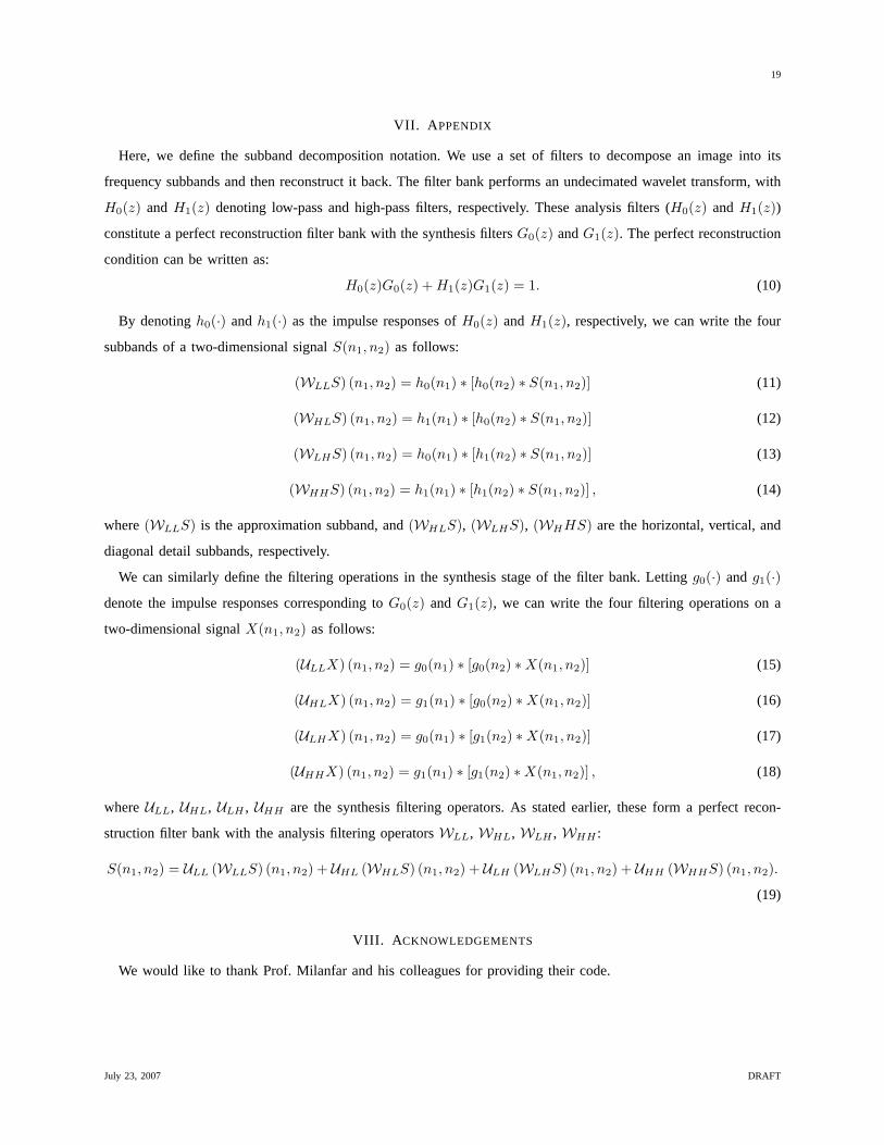
VII. A PPENDIX
Here, we define the subband decomposition notation. We use a set of filters to decompose an image into its
frequency subbands and then reconstruct it back. The filter bank performs an undecimated wavelet transform, with
H0(z) and H1(z) denoting low-pass and high-pass filters, respectively. These analysis filters (H0(z) and H1(z))
constitute a perfect reconstruction filter bank with the synthesis filtersG0(z) andG1(z). The perfect reconstruction
condition can be written as:
H0(z)G0(z) + H1(z)G1(z) = 1. (10)
By denotingh0(·) andh1(·) as the impulse responses ofH0(z) andH1(z), respectively, we can write the four
subbands of a two-dimensional signalS(n1, n2) as follows:
(WLLS) (n1, n2) = h0(n1) ∗ [h0(n2) ∗ S(n1, n2)] (11)
(WHLS) (n1, n2) = h1(n1) ∗ [h0(n2) ∗ S(n1, n2)] (12)
(WLHS) (n1, n2) = h0(n1) ∗ [h1(n2) ∗ S(n1, n2)] (13)
(WHHS) (n1, n2) = h1(n1) ∗ [h1(n2) ∗ S(n1, n2)] , (14)
where(WLLS) is the approximation subband, and(WHLS), (WLHS), (WHHS) are the horizontal, vertical, and
diagonal detail subbands, respectively.
We can similarly define the filtering operations in the synthesis stage of the filter bank. Lettingg0(·) andg1(·)denote the impulse responses corresponding toG0(z) and G1(z), we can write the four filtering operations on a
two-dimensional signalX(n1, n2) as follows:
(ULLX) (n1, n2) = g0(n1) ∗ [g0(n2) ∗X(n1, n2)] (15)
(UHLX) (n1, n2) = g1(n1) ∗ [g0(n2) ∗X(n1, n2)] (16)
(ULHX) (n1, n2) = g0(n1) ∗ [g1(n2) ∗X(n1, n2)] (17)
(UHHX) (n1, n2) = g1(n1) ∗ [g1(n2) ∗X(n1, n2)] , (18)
whereULL, UHL, ULH , UHH are the synthesis filtering operators. As stated earlier, these form a perfect recon-
struction filter bank with the analysis filtering operatorsWLL, WHL, WLH , WHH :
S(n1, n2) = ULL (WLLS) (n1, n2) + UHL (WHLS) (n1, n2) + ULH (WLHS) (n1, n2) + UHH (WHHS) (n1, n2).
(19)
VIII. A CKNOWLEDGEMENTS
We would like to thank Prof. Milanfar and his colleagues for providing their code.
July 23, 2007 DRAFT
20
REFERENCES
[Adams, 1995] Adams, J. E. (1995). Interactions between color plane interpolation and other image processing functions in electronic
photography. InProc. SPIE, volume 2416, pages 144–151.
[Adams and Hamilton, 1997]Adams, J. E. and Hamilton, J. F. (1997). Design of practical color filter array interpolation algorithms for digital
cameras. InProc. SPIE, volume 3028, pages 117–125.
[Capel and Zisserman, 2000]Capel, D. and Zisserman, A. (2000). Super-resolution enhancement of text image sequences. InProc. IEEE Int.
Conf. Pattern Recognition, volume 1, pages 600–605.
[Combettes, 1993]Combettes, P. L. (1993). The foundations of set theoretic estimation.Proc. IEEE, 81(2):182–208.
[Farsiu et al., 2006]Farsiu, S., Robinson, D., Elad, M., and Milanfar, P. (2006). Advances and challenges in super-resolution.IEEE Trans.
Image Processing, 15(1):141–159.
[Freeman, 1988]Freeman, W. T. (1988). Method and apparatus for reconstructing missing color samples.U.S. Patent 4,774,565.
[Gevrekci and Gunturk, 2006]Gevrekci, M. and Gunturk, B. K. (2006). Matlab user interface for super resolution image reconstruction
for illumination varying and Bayer images, Dept. of Electrical and Computer Engineering, Louisiana State University, April 2007
http://www.ece.lsu.edu/ipl/demos.html.
[Glotzbach et al., 2001]Glotzbach, J. W., Schafer, R. W., and Illgner, K. (2001). A method of color filter array interpolation with alias
cancellation properties. InProc. IEEE Int. Conf. Image Processing, volume 1, pages 141–144.
[Gotoh and Okutomi, 2004]Gotoh, T. and Okutomi, M. (2004). Direct super-resolution and registration using raw cfa images. InProc. IEEE
Int. Conf. Computer Vision and Pattern Recognition, volume 2, pages 600–607.
[Gunturk et al., 2002]Gunturk, B. K., Altunbasak, Y., and Mersereau, R. M. (2002). Color plane interpolation using alternating projections.
IEEE Trans. Image Processing, 11(9):997–1013.
[Gunturk et al., 2005]Gunturk, B. K., Glotzbach, J., Altunbasak, Y., Schafer, R. W., and Mersereau, R. M. (2005). Demosaicking: color filter
array interpolation.IEEE Signal Processing Magazine, 22(1):44–54.
[Hibbard, 1995] Hibbard, R. H. (1995). Apparatus and method for adaptively interpolating a full color image utilizing luminance gradients.
U.S. Patent 5,382,976.
[Hirakawa and Parks, 2005]Hirakawa, K. and Parks, T. (2005). Adaptive homogeneity-directed demosaicing algorithm.IEEE Trans. Image
Processing, 14(3):360–369.
[Hirakawa and Parks, 2003]Hirakawa, K. and Parks, T. W. (2003). Adaptive homogeneity-directed demosaicing algorithm.Proc. IEEE Int.
Conf. Image Processing, 3:669–672.
[Irani and Peleg, 1991]Irani, M. and Peleg, S. (1991). Improving resolution by image registration.CVGIP: Graphical Models and Image
Processing, 53:231–239.
[Kapah and Hel-Or, 2000]Kapah, O. and Hel-Or, H. Z. (2000). Demosaicing using artificial neural networks. InProc. SPIE, volume 3962,
pages 112–120.
[Kimmel, 1999] Kimmel, R. (1999). Demosaicing: image reconstruction from ccd samples.IEEE Trans. Image Processing, 8:1221–1228.
[Laroche and Prescott, 1994]Laroche, C. A. and Prescott, M. A. (1994). Apparatus and method for adaptively interpolating a full color image
utilizing chrominance gradients.U.S. Patent 5,373,322.
[Mukherjee et al., 2001]Mukherjee, J., Parthasarathi, R., and Goyal, S. (2001). Markov random field processing for color demosaicing.Pattern
Recognition Letters, 22(3-4):339–351.
[Pei and Tam, 2003]Pei, S.-C. and Tam, I.-K. (2003). Effective color interpolation in ccd color filter arrays using signal correlation.IEEE
Trans. Circuits and Systems for Video Technology, 13(6):503–513.
[Tomasi and Manduchi, 1998]Tomasi, C. and Manduchi, R. (1998). Bilateral filtering for gray and color images. InProceedings of the 1998
IEEE International Conference on Computer Vision, pages 839–846.
July 23, 2007 DRAFT