Embed Size (px)
Citation preview
Responsive Market Regulation in Environmental Economics:An Agent-Based Stochastic Equilibrium Approach
Dissertationzur Erlangung des Doktorgrades Dr. rer. nat.
der Fakultat fur Mathematikder Universitat Duisburg-Essen
vorgelegt vonDipl.-Math. Sascha Kollenberg
aus Aachen
EssenMarz 2018

ii Erstgutachter: Prof. Dr. Rüdiger Kiesel, Universität Duisburg-Essen Zweitgutachter: Prof. Dr. Ralf Werner, Universität Augsburg Datum der Disputation: 25.07.2018

iii
Ich versichere an Eides statt durch meine Unterschrift, dass ich die vorstehende Arbeit selbststandig und ohne fremde Hil-fe angefertigt und alle Stellen, die ich wortlich oder inhaltlich aus Veroffentlichungen entnommen habe, als solche kenntlichgemacht habe, mich auch keiner anderen als der angegebenen Literatur und keinem anderen als der genannten Hilfsmittelbedient habe. Die Arbeit hat in dieser oder ahnlicher Form noch keiner anderen Prufungsbehorde vorgelegen. Es hat kein vor-angegangenes Promotionsverfahren gegeben.
Sascha KollenbergMarz 2018

iv
v
German Summary / Deutsche Zusammenfassung
In der vorliegenden Arbeit beschaftigen wir1 uns mit der stochastischen Modellierung von Markten fur regulierte Ressourcen.Dabei verwenden wir den Begriff der regulierten Ressource (bzw. der regulierten Commodity) im Sinne eines Gutes dessen Gesamt-verbrauch in einer vorher festgelegten Periode durch eine staatliche, zwischenstaatliche oder private, zentrale Entitat gesteuertwird. Zudem soll ein etwaiger Zufluss der Ressource zum Markt durch ebenjene Entitat einer (dynamischen) Regulierung un-terworfen werden konnen. Indem der Zufluss der Ressource zum Markt derart reguliert wird, selbige jedoch anschließend freidurch die Marktteilnehmer gehandelt werden kann, konnen etwaige Externalitaten aus dem Verbrauch der Ressource einge-preist werden, ohne dass der (volks-) wirtschaftliche Schaden aus dem Verbrauch der Ressource selbst quantifiziert werdenmuss.
Ein solches Handelssystem stellt klassischerweise eine Alternative zur Besteuerung als Mittel der Einschrankung des (ver-brauchenden) Einsatzes einer Ressource dar. Die Frage, ob ein wie oben beschriebenes mengenbasiertes Instrument oder einpreisbasiertes Instrument (wie bspw. eine Steuer) im Einzelfall vorzuziehen ist, wurde bereits von [Weitzman, 1974] behandelt,dessen Betrachtungen auf den Vergleich der Steigung marginaler Nutzen- und Kostenkurven bzgl. der Ressourceneinsparunghinausliefen. Weitzman bemerkt jedoch ebenfalls, dass ein ideales Instrument ein dynamisches Signal auf Basis des aktuellenZustandes der Volkswirtschaft senden wurde, fur die oder in der die Regulierung gilt. In der vorliegenden Arbeit greifen wirdiesen Gedanken Weitzmans auf und untersuchen, wie die Kosteneffizienz einer Regulierung durch ein dynamisches Signalgesteigert werden kann. Zudem stellen wir dar, wie dynamische Regulierungen zur Abbildung eines ganzen Spektrums an In-strumenten verwendet werden konnen, welche zwischen den Extremen eines reinen mengen- und eines reinen preisbasiertenInstruments liegen. Die vorliegende Arbeit fullt damit eine nicht unwesentliche konzeptionelle Lucke in der okonomischenLiteratur.
Eine Einschrankung oder Regulierung der Forderung bzw. des Einsatzes einer Ressource kann im kollektiven Interesse ei-ner Gruppe von Wirtschaftssubjekten sein, oder aber im Interesse der Gesellschaft, welche den Folgen des Handelns jenerWirtschaftssubjekte ausgeliefert ist. Wahrend sich Beispiele fur Ersteres vornehmlich im Bereich des Kartellwesens bewe-gen (bspw. Forderung von begrenzten naturlichen Ressourcen wie fossiler Brennstoffe), kommt Letzteres zum Tragen, wennschwerwiegende gesellschaftliche Folgen zu erwarten sind, sollte die Verwendung einer Ressource gewisse Grenzen uber-schreiten. Beispiele fur die Losung einer solchen Problematik finden sich in der Fischerei in Form sogenannter IndividualTransferrable Quotas2 und in der Forstwirtschaft3, wesentlich prominentererweise jedoch auch im Handel von Emissionsrech-ten, welchen wir als wesentliches Anwendungsbeispiel kurz vorstellen wollen.
Unser wesentliches Anwendungsbeispiel fur oben beschriebene regulierte Ressourcen sind klimarelevante Commodities, al-len voran CO2-Emissionsrechte. Solche Emissionsrechte werden in der Europaischen Union seit 2005 unter dem sogenanntenEuropean Union Emissions Trading System (EU ETS) gehandelt. Hierbei werden dem Markt in regelmaßigen Auktionen so-wie durch freie Allokationen Emissionsrechte in Form sogenannter EUAs (European Emission Allowances) zugefuhrt, welcheanschließend frei und zum durch den Markt (endogen) festgelegten Preis gehandelt werden konnen. Die unter das EU ETSfallenden Agenten mussen nun fur jedes Kalenderjahr eine Menge von EUAs vorweisen konnen, welche ihrem Treibhausgas-austoß in Tonnen CO2-Aquivalent (CO2 equivalent, CO2e) entspricht. Zur Anreizsetzung fallt fur jede nicht auf diese Weiseabgedeckte Tonne CO2e eine fixe Strafzahlung von derzeit 100 EUR an. (Es sei angemerkt, dass jeder unter die Regulierungfallende Marktteilnehmer auch nach Zahlung der Strafgebuhr dazu verpflichtet ist, die entsprechende Menge an EUAs in dernachsten Abrechnungsperiode nachzureichen.)
Nach der Wirtschaftskrise 2007/08 trat auf dem europaischen Markt fur Emissionsrechte ein Preisverfall ein, dessen Fol-gen bis heute andauern. Das dem Preisverfall zugrundeliegende Uberangebot an EUAs wird landlaufig weitestgehend ei-ner Produktionseinbuße der unter die entsprechende Regulierung fallenden Wirtschaftssubjekte zugeschrieben. Als Folge deroben genannten Entwicklungen kamen seitens einiger gesellschaftlicher und politischer Interessengemeinschaften Zweifel ander Zulanglichkeit des Regelwerks auf, welches dem EU ETS bis dato zugrunde lag. Es wurde insbesondere moniert, dasderzeitige System ware nicht in der Lage, auf sich andernde okonomische Rahmenbedingungen angemessen zu reagieren.
Aufbauend auf einer auf diese Problematik abzielenden Konsultation von externen Experten und Stakeholdern wurde imNovember 2012 durch die Europaische Kommission ein Ergebnispapier4 veroffentlicht, welches eine Reihe moglicher Maß-nahmen zur Behebung der oben genannten Unzulanglichkeiten des Systems umriss. Unter den genannten Maßnahmen wardie Einfuhrung einer sogenannte Marktstabilitatsreserve (MSR), welche den Zufluss von EUAs zum Markt statt wie bislangstatisch, nunmehr dynamisch gestalten sollte: Die Ausschreibungsmengen sollten sich gemaß dieses Vorschlags an der Mengeder sich im Markt befindlichen (also insbesondere nicht bereits zur Abdeckung von Emissionen verwendeten) EUAs orientie-ren. Zudem sollte diese Zuflussregulierung nach festen und transparenten Regeln geschehen, um politische Risiken im Sinne
1Ich verwende in der vorliegenden Arbeit stets die Formulierung ‘wir’ anstelle von ‘ich’ (bzw. Englisch ‘we’ anstelle von ‘I’) etc. im Sinneeiner sprachlichen Einbindung des Lesers in den Verlauf und Aufbau der Arbeit. Die Eigenstandigkeit meiner zugrundeliegenden Leistungbleibt hiervon unberuhrt.
2Siehe bspw. [Grafton, 1996].3Siehe bspw. [Teeguarden, 1969].4Siehe [The European Commission, 2012].
vi
der Marktteilnehmer einzudammen. Die MSR wurde im Jahr 2016 ratifiziert und wird nach derzeit geltender Rechtsprechungab 2020 aktiv.
In der vorliegenden Arbeit konstruieren wir ein zeitstetiges stochastisches Gleichgewichtsmodell eines Marktes fur regulier-te Ressourcen, mit besonderem Augenmerk auf obigem wesentlichem Anwendungsbeispiel. Wir legen hierbei insbesondereWert auf eine mathematisch rigorose Abbildung von Risikoaversion auf Seiten der Marktteilnehmer, sowie eine detaillierteAusarbeitung einer Losung des Gleichgewichtsproblems in geschlossener Form. Es gelingt uns insbesondere, das fur jeden ein-zelnen Marktteilnehmer auftretende Optimierungsproblem, zusammen mit der damit assoziierten Hamilton-Jacobi-Bellman-Gleichung explizit zu losen. Anschließend konstruieren wir einen Mechanismus zur dynamischen Kontrolle des Ressourcen-zuflusses, welcher, aufbauend auf unserem Gleichgewichtsmodell, eine Losung des Marktgleichgewichtes unter jener Regu-lierung zulasst. Es gelingt uns damit auch, die Wechselwirkung zwischen der dynamischen Regulierung (deren Signal auf derMarktsituation beruht) und der Marktdynamik (dessen Entwicklung von der dynamischen Regulierung abhangt) darzustellenund eine entsprechende Gleichgewichtslosung zu finden. Dadurch gelingt es uns wiederum, die Kosteneffizienz des Systemsexplizit zu quantifizieren womit wir zeigen, wie ein solches dynamisches System hinsichtlich der Kosteneffizienz zu optimie-ren ist. Wir stellen dabei fest, dass ein dynamisches System durch Reduktion der Kosten, welche seitens der Marktteilnehmerdurch Anpassung an stochastische Einflusse entstehen, einem statischen System uberlegen sein kann – und zwar insbesondereauch dann, wenn dem Markt in Erwartung weniger Ressourceneinheiten zur Verfugung gestellt werden als dies ohne einedynamische Angebotsanpassung der Fall ware.
Durch die Allgemeinheit unseres Vorgehens gelingt es uns außerdem, das eingangs erwahnte Spektrum zwischen reinenmengen- und reinen preisbasierten Instrumenten zur Regulierung des Ressourceneinsatzes abzubilden: Mithilfe einer einfa-chen Parametrisierung der Responsivitat des Mechanismus offenbart sich eine vollstandige abstrakte Darstellung des Konti-nuums von Instrumenten. Damit adressieren wir mit unserer Analyse nicht nur die Frage nach einem optimalen dynamischenAllokationsmechanismus, sondern vielmehr auch die Frage nach einer optimalen Politikgestaltung durch gemischte Preis-und Mengensysteme. Damit schließen wir eine wesentliche konzeptionelle Lucke in dem durch [Weitzman, 1974] eingeleitetenZweig der okonomischen Literatur.
Unsere Arbeit gliedert sich in vier Kapitel. In Kapitel 1 beschreiben wir unsere Motivation und ordnen unsere Arbeit in denKontext der okonomischen Literatur ein. Es folgen in Kapitel 2 einige allgemeine Bemerkungen und Ergebnisse zu unseremstochastischen Modellierungsansatz. In Kapitel 3 erfolgt nun die Konstruktion unseres stochastischen Gleichgewichtsmodellssowie dessen explizite Losung. Anschließend wird in Kapitel 4 der Mechanismus zur dynamischen Allokation spezifiziertund das resultierende Marktgleichgewicht dargelegt. Wir legen hier außerdem dar, wie die aggregierten Kosten berechnet undminimiert werden konnen. Wir gehen hier ebenfalls detailliert auf das eingangs genannte Spektrum von Instrumenten ein, undwie es anhand der Parametrisierung unseres dynamischen Mechanismus abgebildet werden kann.
Einige der in den Kapiteln 3 und 4 prasentierten Ergebnisse wurden von mir in kurzerer und vereinfachter Form in [Kollenberg and Taschi-ni, 2016a] sowie [Kollenberg and Taschini, 2016b] veroffentlicht. Dies beinhaltet insbesondere die im letzten Kapitel gezeigten Abbildungen5
4.1, 4.2 und 4.3.
5Der den Abbildungen zugrundeliegende Programmcode wurde von mir eigenstandig in der zu MathWorks Matlab gehorenden, pro-prietaren Sprache geschrieben. Die genannten Abbildungen habe ich mittels Matlab unter einer gultigen Lizenz selbstandig erstellt.
vii
English Summary
The present work is concerned with stochastic modelling of markets for regulated resources. Here, we6 use the term regulatedresource (or regulated commodity) in the sense of some tradable good, the total aggregate deployment of which is subject to con-trol by some public or private, central entity. More precisely, we are interested in regulatory systems that can control the inflowof commodity units. Such control systems allow the regulator to force potential externalities, arising from using the resource,to be priced in on the market, without explicitly deciding on the respective premium or explicitly quantifying the economicdamage avoided for each unit of the commodity.
Such (quantity-based) trading systems are traditionally viewed as alternatives to conventional price-based systems such astaxes. The question whether a quantity-based or price-based system is more advantageous has first been studied by [Weitzman,1974], whose deliberations came down to comparing the relative slopes of the marginal abatement cost curve and marginal ben-efit curve (of avoiding emissions). However, Weitzman appreciated that an ideal instrument would implement a contingencymessage, indicating what policy would be implemented, based on the current state of the system. In the present work, we pickup on this idea and examine how the costs efficiency of controlling the use of a resource can be improved by such dynamiccontrol systems. What’s more, we construct a quantitative framework by which we can represent an entire spectrum of policiesbetween ‘pure’ price-based and ‘pure’ quantity-based instruments. Thusly we fill a significant gap in the pertinent literature.
Limitation or regulation of the inflow of commodity units to some economy can be in the collective interest of a group ofeconomic entities, or in the interest of the society which is subjected to those entities’ externalities. While examples for theformer are mainly found in the context of cartels, the latter is relevant whenever societal damages are the result of the con-sumption of a commodity – e.g. through overfishing or non-sustainable forestry. Another, particularly topical example areclimate relevant commodities such as fossil fuels or emissions allowances.
The main inspiration for our modelling work are Emissions Trading Systems (ETSs), the currently largest of which is theEuropean Union ETS (EU ETS). Therein, emissions allowances (EUAs – European Emission Allowances) are made availableby the regulator through regular auctions and free allocations. Those allowances can then be traded freely among marketparticipants at the price dictated only by supply and demand on this secondary market. After a given calendar year, agentswhose facilities are subject to the regulation of the EU ETS have to present a number of EUAs equal to their total emissionsof greenhouse gases, measured in (metric) tonnes of CO2-equivalent (CO2e), during the respective year. For each tonne notcovered in this way, each agent who is short in allowances has to pay a penalty of (currently) 100 Euros. (It shall be mentionedthat paying the penalty does not absolve the agent from having to present the respective allowances in the next year.)
In the wake of the economic crisis of 2007/08, we saw a strong and persistent erosion of EUA prices, which is mainly at-tributed to an oversupply resulting from an unanticipated drop in production. It was this price erosion, along with the ETS’slack of provisions to adapt to such circumstances, that brought about doubt in the efficacy of the instrument altogether. Moreprecisely, a number of experts in academia, politics and some stakeholders believed that the system was unable to ‘functionin an orderly fashion’ [The European Commission, 2012] in the presence of such an enormous oversupply. In particular, thesystem lacked provisions to adapt the allocation scheme to changes in economic circumstances.
Based on public consultations, the European Commission released a report in November 2012 (see [The European Commission,2012]), presenting a number of reform options for the EU ETS, which aimed at relieving the current oversupply and, poten-tially, making the system more responsive to changes in economic circumstances. One such measure is the introduction ofthe so-called Market Stability Reserve (MSR), which aims at making the supply of allowances dynamic and dependent on thestate of the system, rather than static and rigid, as it was. Furthermore, this supply adjustment system is designed based on atransparent set of rules, rather than discretionary interventions. The MSR has been ratified in 2016 and is set to start operatingin 2020.
In the present work, we construct a continuous-time stochastic equilibrium model of a market for an abstract regulated com-modity, with special interest in applications to climate-relevant resources such as emissions allowances. In doing so, we putspecial emphasis on a mathematically rigorous representation of stochasticity and risk-aversion on behalf of market partici-pants, as well as on a detailed (agent-based) derivation of the equilibrium dynamics in closed-form. In the process, we solveeach agent’s optimisation problem, along with the associated Hamilton-Jacobi-Bellman Equation, for which we are able to findan explicit solution. Furthermore, we construct a generic regulatory mechanism of dynamic resource allocation, similar inspirit to the Market Stability Reserve. Our dynamic regulatory mechanism adjusts the resource allocation based on the currentsystem state. The system state, however, is dependent on the allocation scheme, which implies the existence of a feed-backloop between the market and the regulation. We are, notably, able to solve this inter-dependency and derive the equilibriumunder this regulation. This in turn allows us to quantify the costs associated to any given parameterisation of the mechanism,adjusting its responsiveness in order to maximise the cost-efficiency of the system. What’s more, by employing an adjustableresponsiveness, we are able to represent an entire spectrum of policies between pure price instruments and pure quantity in-struments. Thereby, we fill a significant gap in the stream of literature pioneered by [Weitzman, 1974].
The present text is divided into four chapters. In Chapter 1 we describe our motivation along with the literature context of
6Throughout the text, I use the term we instead of I etc. in the sense of ‘guiding the reader through the text’. This formulation does notimply that I had any unwarranted assistance for my work. Accordingly, the independence of my efforts remains unaffected by such or similarformulations.

viii
our work. In Chapter 2 we present some general concepts and observations on stochastic equilibria which will prove useful forour modelling approach. In Chapter 3 we derive our equilibrium in closed-form, before we construct our dynamic regulatorymechanism in Chapter 4. Therein, we furthermore compute total aggregate abatement costs as a function of the responsivenessof the system. This allows us to present means for the construction of a mechanism that maximises the policy’s cost-efficiency.We also provide an in-depth analysis of how the above-mentioned spectrum of policies can be represented by our mechanism’sparameterisation.
Some of the results presented in this text have been published by the author in a more compact and somewhat simplified fashion in [Kollenbergand Taschini, 2016a] and [Kollenberg and Taschini, 2016b]. This pertains in particular to Chapters 3 and 4; and specifically to Figures7
4.1, 4.2 and 4.3.
7The code by which the figures have been generated is written by me in MathWorks Matlab’s proprietary language. I have used Matlab togenerate these figures under a valid licence.

ix

x
Contents
1 Motivation and Context 11.1 Responsive Policies in Environmental Economics . . . . . . . . . . . . . . . . . . . . . . . . . . . . . . . . . . . . . . 11.2 Topical Inspiration: The European Carbon Market . . . . . . . . . . . . . . . . . . . . . . . . . . . . . . . . . . . . . 21.3 Responsiveness and Price- vs. Quantity-Instruments . . . . . . . . . . . . . . . . . . . . . . . . . . . . . . . . . . . . 21.4 The Trade-Off Between Flexibility and Reduced Uncertainty . . . . . . . . . . . . . . . . . . . . . . . . . . . . . . . 3
2 Market Equilibria 52.1 First- and Second-Level Uncertainty . . . . . . . . . . . . . . . . . . . . . . . . . . . . . . . . . . . . . . . . . . . . . 72.2 Strong and Weak Equilibria . . . . . . . . . . . . . . . . . . . . . . . . . . . . . . . . . . . . . . . . . . . . . . . . . . 72.3 Risk-Aversion . . . . . . . . . . . . . . . . . . . . . . . . . . . . . . . . . . . . . . . . . . . . . . . . . . . . . . . . . . 9
3 A Stochastic Equilibrium Model 113.1 Deployment, Abatement and Trading . . . . . . . . . . . . . . . . . . . . . . . . . . . . . . . . . . . . . . . . . . . . 113.2 Required Abatement and the Bank of Commodity Units . . . . . . . . . . . . . . . . . . . . . . . . . . . . . . . . . . 123.3 Instantaneous and Inter-Temporal Optimisation . . . . . . . . . . . . . . . . . . . . . . . . . . . . . . . . . . . . . . 143.4 Equilibrium in the Deterministic Case . . . . . . . . . . . . . . . . . . . . . . . . . . . . . . . . . . . . . . . . . . . . 173.5 Strong Equilibrium under a Risk-Neutral Measure . . . . . . . . . . . . . . . . . . . . . . . . . . . . . . . . . . . . . 20
3.5.1 Technical Preliminaries: Optimal Stochastic Control . . . . . . . . . . . . . . . . . . . . . . . . . . . . . . . . 203.5.2 Explicit Solution of each Agent’s Hamilton-Jacobi-Bellman Equation . . . . . . . . . . . . . . . . . . . . . . 243.5.3 Verification Theorem . . . . . . . . . . . . . . . . . . . . . . . . . . . . . . . . . . . . . . . . . . . . . . . . . . 30
3.6 Uniqueness of the Equilibrium . . . . . . . . . . . . . . . . . . . . . . . . . . . . . . . . . . . . . . . . . . . . . . . . 353.7 Weak Equilibrium Property under the Objective Measure . . . . . . . . . . . . . . . . . . . . . . . . . . . . . . . . . 35
4 Policy Relevance and Application 374.1 Cap Stringency and Responsiveness . . . . . . . . . . . . . . . . . . . . . . . . . . . . . . . . . . . . . . . . . . . . . 374.2 A Regulatory Mechanism with Adjustable Responsiveness . . . . . . . . . . . . . . . . . . . . . . . . . . . . . . . . 384.3 Expected Total Abatement Costs and Policy Implications . . . . . . . . . . . . . . . . . . . . . . . . . . . . . . . . . 42
4.3.1 The Optimal Adjustment Rate . . . . . . . . . . . . . . . . . . . . . . . . . . . . . . . . . . . . . . . . . . . . 444.3.2 The Effects of the Adjustment Rate on the Risk Premium . . . . . . . . . . . . . . . . . . . . . . . . . . . . . 45
4.4 Conclusions . . . . . . . . . . . . . . . . . . . . . . . . . . . . . . . . . . . . . . . . . . . . . . . . . . . . . . . . . . . 47
xi

xii CONTENTS
Chapter 1
Motivation andContext
In this chapter, we will present the motivation for our quanti-tative work and its context in climate economics. As we shallsee in Chapters 2 and 3, our model supports a wide variety ofapplications in the context of regulated commodities. How-ever, we draw our inspiration specifically from commoditieswhich are climate relevant due to the greenhouse gas emis-sions originating from their deployment in the production ofgoods and services. More specifically, we address the questionof how the deployment of such resources can be limited cost-efficiently by implementing a responsive system of regulatorycontrol.1
1.1 Responsive Policies in EnvironmentalEconomics
In the wake of the crisis that started in 2007 and shook thefinancial system to its core, we saw a surge in academic inter-est in how the risk of economic shocks should be incorporatedin climate change policies. This particularly concerns instru-ments which aim at charging economic entities for the burdenthey impose onto society due to their greenhouse gas emis-sions. In economic terms, all such instruments have in com-mon that they implicitly or explicitly put a price on that ex-ternality. Since greenhouse gases are commonly measured interms of their contribution to climate change, relative to that oftonnes of CO2, we refer to any such measure as a carbon pricinginstrument.
Two such carbon pricing instruments have been of particularinterest in the pertinent literature. These are Emissions Trad-ing Systems (ETSs) on the one hand, and simple taxation onthe other hand. We shall see that in many ways, these two op-tions represent two poles at the edges of an entire spectrum ofpossible instruments: Situated on what we will refer to as thequantity extreme of this policy spectrum lies a pure ETS; i.e. anemissions trading system with a fixed cap2 and a fixed allo-cation schedule that will not be altered ex-post. The idea of
an ETS exhibits a strong conceptual appeal which makes itparticularly popular among economists: In any ETS, the reg-ulator makes a number of allowances available at differentpoints in time. This may be done via free allocation, regularauctions, or a combination of the two. In a pure ETS, the to-tal number of allowances that will be made available is finiteand pre-determined by the regulator. At predefined intervals,the regulated entities have to present a number of allowancesthat suffice to cover their emissions during the respective time-frame. By means of banking and borrowing provisions3, theregulated entities are provided with some degree of temporalflexibility, in addition to the spacial flexibility from being ableto trade allowances amongst each other.4 If adequately en-forced (e.g. by sufficient penalties for non-compliance), the to-tal number of allowances available (the cap) ensures that totalemissions remain below a fixed ceiling. This relative certaintyof ecological efficacy, paired with the cost-efficiency providedby spacial and temporal flexibility, make for the strong appealof an ETS – in particular among economists. With the intro-duction of the European Union Emissions Trading System (EUETS) in 2005, which is still the largest system of its kind, theconcept of an ETS has found a strong flagship implementation,albeit suffering criticism and some considerable opposition.
On the other end of the policy spectrum, which we will referto as the price extreme, lies pure carbon taxation; i.e. a fixedprice or price trajectory is put on carbon, whereas the totalamount of emissions is theoretically unbounded and subjectto the taxed entities’ decision making: The regulated agentssimply assess their marginal benefit from emissions versus thestipulated tax, but no definitive maximum on their aggregateemissions is prescribed. However, this instrument has the ad-vantage of being more straightforward in its concept and real-isation. Furthermore, the idea of a carbon tax has a somewhatstrong backing, not least from environmentalist groups, seek-ing a more direct and controllable form of a financial burdento be imposed on ‘culprit companies’.
Pure quantity-based instruments such as emissions-tradingsystems with a fixed cap, and pure price-based instrumentssuch as fixed taxes have been juxtaposed in a seminal paperby [Weitzman, 1974]. These two policies are characterised byeither imposing a fixed total reduction quantity (via the cap)with a fully floating price (meaning the price is determined bythe market and there is no ex-post adjustment to the cap), or byimposing a fixed price for the commodity which can (in the-ory) be set to induce any desired (expected) reduction quan-tity. In a deterministic world, the outcome of each of thoseinstruments can be replicated by the other with an appropri-ate parameterisation (cap or tax level): In a stylised setting,where marginal abatement cost curves and marginal benefitcurves are known and certain, a tax could be set to induce anydesired emissions level, which in turn could be set to induceany desired price. However, under uncertainty, the two instru-ments are not necessarily perfectly equivalent and the choiceof one over the other is essentially reduced to comparing therelative slopes of the marginal benefit curve (of reducing emis-
1Some of the results presented in this text have been published by the author in a more compact and somewhat simplified fashion in [Kol-lenberg and Taschini, 2016a] and [Kollenberg and Taschini, 2016b]. This pertains in particular to Chapters 3 and 4 and the figures presentedtherein.
2As is conventional, we refer to the total number of commodity units (e.g. emissions allowances) issued over the entire regulated timeframesimply as the cap of the regulated system.
3As is conventional, we often use the term (net-)banking to describe an agent’s decision to keep commodity units allotted or purchased atone point of time in order to use them later-on. The term (net-) borrowing, on the other hand, describes an agent’s act of using more allowancesat one point in time than are currently in the agent’s stock. We will provide more details on how agents can use commodity units in Chapter 3,where we introduce the notions of deployment and abatement.
4We will provide more details on the flexibilities provided to regulated agents and their significance in Section 1.4.
1
2 CHAPTER 1. MOTIVATION AND CONTEXT
sions) and of the marginal abatement cost curve [Weitzman,1974]. Whats more, the two instruments are taken to be non-responsive in the sense that the cap or tax rate is not adjustedin response to the ex-post observed outcome over time. In ouranalysis, we move away from a Weitzmanian comparison be-tween individual pure instruments, i.e. price vs. quantity, andfocus our attention towards the notion of responsiveness inETSs and hybrid systems. Our approach is based on the un-derstanding that, in analogy to monetary policy, a rigid ex-ante ETS cap may turn out to be too lenient during an eco-nomic recession and too strict in times of economic expansion.Accordingly, we add to the literature by confirming this intu-ition and showing in a rigorous quantitative way, how to re-veal the ‘sweet spot’ in terms of expected cost-efficiency, whentime, uncertainty, and risk-aversion are taken into account.
We will go into more detail on the topic of responsiveness andits relation to price- vs. quantity instruments in Section 1.3.However, in order to illustrate our motivation and the topical-ity of the subject matter, we first consider the present state ofthe currently largest ETS. This will, in particular, shed light onwhy the matter of responsiveness gained some considerableinterest within the realm of climate economics.
1.2 Topical Inspiration: The European Car-bon Market
The economic efficiency and ecological effectiveness of climatepolicy instruments can be greatly influenced by business cy-cles and unanticipated technological developments. Further-more, overlapping policies can hinder each other in their ef-ficacy, evidence of which can be found in the EU ETS: Theerosion of prices for European Emissions Allowances (EUAs)in recent years has, at least partially, been attributed to con-current policies such as feed-in tariffs for renewables. In ad-dition, the system has been shown to suffer from a system-atic unresponsiveness towards large-scale economic shocks,as impressively evidenced during the financial crisis and offi-cially recognised by [The European Commission, 2012]. Thesetwo effects are what the drop and continuing low level of al-lowances prices since 2008 have primarily been attributed to.([Grosjean et al., 2014] and [Ellerman et al., 2015a]).
To address the current situation on the European carbonmarket, which European authorities described as a ‘struc-tural supply-demand imbalance’ [The European Commission,2012], consultants to the EU regulators have proposed a num-ber of plans, two of which have been made applicable legis-lation. The first such measure, labeled ‘back-loading’, tem-porarily offsets a portion of the issued allowances from theallocation schedule, to be definitively re-introduced later-on.In 2016, a second measure, called the ‘Market Stability Re-serve’ (MSR) has been put into place and will start operat-ing in 2020: Aiming to make the system “more resilient tosupply-demand imbalances so as to enable the ETS to functionin an orderly fashion” [The European Parliament and Council,2015], the MSR is a much broader approach to binding the al-lowance supply to the economic development: The MSR willadjust the allowances allocation based on the current number(‘bank’) of unused allowances in circulation. More precisely,the MSR will withdraw a number corresponding to 12% ofthe current bank from next year’s auction quantity if the cur-rent year’s bank lies above 833 Million allowances. These al-lowances will then be placed in a so-called reserve and will bere-introduced to the market in batches of 100 million per year,
should the bank fall below 400 million allowances. Notwith-standing these system-state-based allocation adjustments, theMSR may not be able to make the system fully responsive to ex-ternal shocks, since the total cap over the regulated timeframemay be perceived to remain unaltered in expectation ([Perinoand Willner, 2015] and [Kollenberg and Taschini, 2016b]). Inthis sense, the MSR can be seen as a partially responsive sys-tem, closely related, but not identical to systems with a fullyfloating cap. This is because the MSR does provide for someresponsiveness, albeit potentially with only temporal effects:Even though there is no definitive timeline as to when al-lowances that have been withdrawn are re-introduced, even-tually the reserve may well be expected to run out, reinstatingthe ex-ante cap.
Inspired by these shortcomings, we will consider a spectrum ofpolicies, from non-responsive to fully responsive, where thecap may be altered, in order to study how different gradesof responsiveness can benefit the system in terms of cost-efficiency.
1.3 Responsiveness and Price- vs. Quantity-Instruments
Taking the EC MSR as an inspiration, we will construct ageneric supply control mechanism which is applicable to bothphysical resources and tradable externalities (such as emis-sions allowances): Regarding physical resources, the regula-tor may, for example, control the extraction of a resource bysetting yearly quotas, based on the market-wide bank. In fact,the application of (discretionary) quotas is common practicein the regulation of renewable resources, as evidenced by in-dividual transferable quotas in fishery [Grafton, 1996] or cut-ting quotas in forestry [Teeguarden, 1969]. Extraction quotasfor non-renewable resources such as oil, on the other hand, areoften subject to cartel interests which may not cover ecologicalobjectives [Bain, 1948]. The present text abstracts away fromthe specifics of an individual class of resources but focuses onthe matter of responsively regulating a group of agents whomay deploy and trade a resource based on their individual in-centives.The concept of a responsive policy represents a well-established idea among economists. In his seminal paper onthe subject of quantity- vs. price-based instruments, [Weitz-man, 1974] appreciates that an optimised instrument of con-trolling a scarce resource or externality would implement acontingency message, indicating which realisation of the pol-icy would be taken into action, depending on the realised stateof the market and the economy. For example, the number oftradable units of the regulated commodity that are made avail-able to the market, may be made dependent on some referencequantity that reflects the state of the system with respect toeconomic or ecological aspects. Often times, though, such con-tingent policies may be hard to bring forward in the legislativeprocedure. Nevertheless, in other than climate-related areasof quantity-based regulation, this impediment does not existacross the board: Central banking, for example, relies stronglyon the adjustment of interest rates to be set in response toeconomic cycles. Seen from this perspective, a system-state-dependent regulation is not at all just an idealising concept,but very much a concrete example of applicable economic the-ory. In appreciation of supposed barriers of implementingcontingent mechanisms and in light of the novelty of his ap-proach, [Weitzman, 1974] concentrated his analysis on singleorder policies. In the present text, we pick up on his ideas
1.4. THE TRADE-OFF BETWEEN FLEXIBILITY AND REDUCED UNCERTAINTY 3
and examine a spectrum of policies between the pure-priceand pure-quantity extremes, simultaneously covering respon-siveness over time and across different possible states of thesystem. In doing so, we take into account the issues of uncer-tainty and risk-aversion, which will prove vital to the devel-opment of an ideal policy.
Recent contributions to the literature on climate policy havehelped a great deal in understanding responsiveness and thelack thereof in current legislative systems. We refer to [Doda,2016] for a rather comprehensive review of the literature onstate-based policies. In anticipation of our modelling sections,we point out that our generic mechanism takes the numberof unused commodity units as its reference state-dimension.Other such dimensions may include e.g. intensity targets5 orindices that reflect the state of the entire economy in the formof some quantitative aggregator (for example the gross domes-tic product of the regulated economy). Regarding climate pol-icy cyclability, we refer to [Heutel, 2012] and [Golosov et al.,2014], while indexing rules have been studied by [Jotzo andPezzey, 2007], [Ellerman and Wing, 2003] and [Newell andPizer, 2008], among others.
Other approaches to establishing responsiveness in an ETS in-clude the combination of quantity- and price-based measuresinto so-called ‘hybrid systems’, a possibility first pointed outby [Roberts and Spence, 1976]. As for an example for suchcombined instruments, price ceilings and floors can be intro-duced to an ETS by adjusting the amount of allowances sup-plied by the regulator in response to changes in the price level.Strict enforcement of such price bounds of course requires theregulator to be able to adjust the cap: Theoretically, if mar-ket fundamentals where able to drive the price upwards il-limitably, then upwards-cap adjustments would need to beunlimited in order to adhere to a strict price ceiling. Con-versely, strict price floors could only be established if the reg-ulator were given the authority to completely remove any un-used allowances from the system. A number of publicationsrevealed that hybrid systems can offer a benefit in terms ofwelfare over pure price and pure quantity instruments.6 Inthe present text, we focus on quantity-based allocation adjust-ment mechanisms, which are similar in spirit to hybrid sys-tems that offer brice-based adjustments of the allocation quan-tity. We will see that quantity-based allocation adjustmentmechanisms can outperform both fixed-cap and fixed-price in-struments (in terms of expected compliance costs).
The present work ties up the literature on both responsive-ness as well as price- vs quantity instruments by filling in theblanks between the pure varieties of these two instruments –with special attention to the role of uncertainty. By consid-ering a generic mechanism, the cap-stringency7 of which canbe adjusted, a continuous spectrum of responsiveness can beachieved: This spectrum lies between a pure quantity instru-ment (a standard ETS with a fixed cap and a fully floatingprice) and a pure price instrument (a fixed carbon tax trajec-tory with a fully floating cap). On the one end of the spectrumlies a mechanism that is completely non-responsive towardsexternal shocks and leaves the cap unaltered. In other words,
it exhibits full cap stringency and we end up with a standardETS – a pure quantity instrument. On the other end of the spec-trum lies a mechanism that is fully responsive and completelyoffsets external shocks, ultimately inducing a fixed price tra-jectory at the expense of altering the ex-ante cap to a poten-tially unlimited extend. Hence, we end up with a de-facto tax– a pure price instrument. We will see that when designing aregulatory framework to the end of limiting the consumptionof a scarce resource or restricting an externality (at minimaleconomic costs), our approach reveals an inherent trade-offbetween the flexibility provided by an ETS and the reductionof uncertainty that elements of price-based policies can pro-vide. We will go into more detail on this concept in Section1.4.
1.4 The Trade-Off Between Flexibility andReduced Uncertainty
Compliance cost minimisation on behalf of agents under anETS regulation is achieved in two ways: On the one hand,spacial flexibility is provisioned by the agents’ ability to freelytrade allowances amongst each other, which lets each agentadjust the amount of allowances to be taken from one point intime to the next without having to provide the necessary dif-ference in its bank only by emissions abatement and deploy-ment of allowances. By means of trading allowances, agentscan thus benefit from their individual cost differences at anypoint in time, allowing them to perform an instantaneous op-timisation. On the other hand, and connected to this provi-sion, an ETS typically provides some temporal flexibility. Thatis, agents can, to some extend, choose the when of their abate-ment and trading decisions, within the bounds dictated bycompliance requirements. In terms of their number of un-used allowances, the regulator typically provides some rangewithin which banking and borrowing of allowances is permit-ted. In that sense, each agent can optimise its decisions overthe entire regulated period by choosing an optimal bankingpath, subject to regulatory constraints, and the agent’s owninstantaneous optimisation.
When risk-averse agents are faced with uncertainty, theirinter-temporal optimisation problem is affected by how riskyan investment in carbon-reduction is. Accordingly, the agents’respective banking curves will be skewed, compared to whatwould be optimal under risk-neutrality. This can have a po-tentially dramatic effect on the cost-efficiency of any systemwhere the aggregate banking curve is not fixed. Fixing thebanking curve, on the other hand, limits the inter-temporaloptimisation opportunities on behalf of the regulated agents.
The above phenomenon inspires us to consider a genericmechanism that adjusts the allocation of allowances based onthe current aggregate bank of unused allowances. In doing so,we leave a degree of freedom that allows us to represent theentire policy spectrum between pure price- and pure quantity-instruments: Each point on the policy spectrum will be char-acterised in terms of a parameter which we will call the al-lowance allocation adjustment rate. This parameter will deter-
5In this context, the term intensity usually refers to carbon-intensity of economic output. For example, we may consider a proxy for thetonnes of CO2e emitted per EUR of gross domestic product.
6See e.g. [Unold and Requate, 2001], [Pizer, 2002], [Hepburn, 2006], [Fell and Morgenstern, 2010],[Grull and Taschini, 2011], and [Fell et al., 2012].
7We use the term cap-stringency when referring in a qualitative sense to how strictly the regulator maintains the ex-ante cap. The quantitativeparameterisation of the policy will be done through what we will refer to as an adjustment rate, which will quantify the level of responsivenessof a given policy. As it will turn out, the terms cap-stringency and responsiveness represent complementary notions. We refer to later chapters fordetails.
4 CHAPTER 1. MOTIVATION AND CONTEXT
mine the rate by which new allowances are made available orunused allowances are removed from the allocation scheme,based on the current number of unused allowances in the sys-tem. In doing so, the rate will alter the stochastic distributionof the bank of unused allowances, tightening it towards oneend of the spectrum (towards a pure price instrument) andloosening it towards the other end (towards a pure quantityinstrument).
Based on our model developed in Chapter 3, we subsequentlydevote Chapter 4 to analysing in depth, how different levelsfor the adjustment rate affect the agents’ banking behaviouralong with aggregate costs. However, in order to motivate ourapproach, we briefly sketch the relevant intuition in the fol-lowing.
When the adjustment rate is increased in favour of a more re-sponsive policy, agents’ inter-temporal cost-saving opportuni-ties are reduced in favour of a market price less susceptibleto external shocks. In other words, if the system moves awayfrom a pure quantity instrument, the free-floating property ofthe bank is restrained and shocks are absorbed by the regula-tor to a larger degree. In particular, when the cap-stringencyis fully relaxed and the system is fully responsive, exogenousshocks are perfectly offset by changes to the allocations andagents’ expectations about their future required abatementdo not change throughout the regulated period. As a result,a fixed price trajectory is induced and we obtain a de-factotax-like system: When market shocks are perfectly offset bychanges to the cap, expectations about future required abate-ment do not change due to exogenous shocks.
With this in mind, a responsive mechanism which adjusts al-lowance allocation based on the current aggregate bank of al-lowances may deeply affect the behaviour of regulated agents:In fact it may constrain agents’ banking behaviour to such anextend that the benefit it provides by lowering the impact ofexternal shocks is hypercompensated by the limitation it im-poses on inter-temporal cost-saving opportunities.
In Chapters 3 and 4, we quantify this relationship to the endof exposing a trade-off along the spectrum and showing thatthere is indeed an optimal policy, which lies not necessarilyon the one nor the other end of the policy spectrum but mayimply a mixed policy to be ideal. We shall see that the timecomponent as well as uncertainty is vital to this insight as wellas to our conclusions in terms of an optimal policy.
Before we develop our model and derive our policy implica-tions, we will devote Chapter 2 to making some general as-sumptions and observations.
Chapter 2
Market Equilibria
Practitioners and academics in economics and financial math-ematics are often interested in finding projections of futuredevelopments on markets for specific commodities and howthese developments may be affected by regulatory interven-tion. Such regulation problems are particularly relevant in en-vironmental economics, where an unregulated economy mayconsume more of a commodity, or impose more externalitiesonto society, than is in society’s own interest, both today andin the distant future.
On the quantitative side, markets pertaining to a specific com-modity or externality are typically modelled with the intentionof inferring projections of future developments under differ-ent regulatory schemes. From a regulatory perspective, wemay for example be interested in finding the best availabletrade-off between the benefit we obtain from the present con-sumption of a commodity on the one hand, and the damage itdoes to future generations on the other hand. Here, the dam-age may be inflicted either by reducing the stock of the com-modity available for future consumption, or by the environ-mental damages incurred from its consumption today. Thisperspective has been taken in a stream of literature pioneeredby [Hotelling, 1931], whose main area of interest lay in theoptimal temporal distribution of consumption from a societalperspective.
This societal inter-temporal trade-off breaks down, however,in in the context of of anthropogenic climate change: One theone hand, catastrophic damages are expected to occur, shouldthe cumulated ‘consumption’ of a commodity, namely an at-mosphere with acceptable levels of greenhouse gases, exceeda certain threshold: By the special nature of climate-relevantcommodities, it is imperative and without alternatives to ob-serve certain limits on this ‘consumption of clean air’. Onthe other hand, CO2 and similar greenhouse gases are whatis commonly referred to as a stock pollutant, meaning in partic-ular, that the marginal societal benefit of emitting less green-house gases can be regarded as negligibly small, compared tothe economic costs of reducing the same amount (as long ascatastrophic damages are avoided).1
The present work is therefore set to explore how thedeployment of resources entailing the emission of green-house gases can be regulated with minimal expected economiccosts. Furthermore, our work incorporates particularly rel-evant challenges faced by the regulator, such as long time-frames and severe economic uncertainties.
A natural and common approach to modelling markets forany type of commodity relies on the notion of a (Nash-type)market equilibrium; that is, a collection of strategies, each forone agent, such that none of the agents has an incentive to in-dividually deviate from its strategy. As simple examples2 suf-fice to show, equilibria are, in general, by no means a guaran-tor of cost-efficiency or collective optimisation. In that sense,the entirety of agents may have an incentive to deviate fromits collection of individual strategies, while each individualmay not. The Nash-type concept of market equilibria there-fore reflects how social and economic catastrophes can be theresult of individual optimisation - a phenomenon which maystrongly suggest regulatory intervention, be it discretionary orbased on a transparent set of rules.
Besides their general conceptual appeal, Nash-type equilibriaare a straightforward choice in particular for approaching reg-ulatory problems, since each agent typically observes a marketstate which can be affected by regulation. In the present work,we will use the classical notion of a Nash-type equilibrium,garnished with some useful complications such as continuoustime and stochasticity. Thereby, we can observe the reactiona specific policy may induce on behalf of market participants.In Chapter 3 we will develop such an equilibrium model andsolve it in closed-form, where the system state (process) maybe affected by regulatory intervention. In Chapter 4 we willimpose a generic regulatory policy to obtain the equilibriumunder regulation. Therein, the regulatory policy is made de-pendent on the (system) state process itself, which impliesthe existence of a feed-back loop between the market and itsregulation. In Chapter 4, we solve this interdependence anddraw some policy conclusions which are particularly relevantin light of the recent reform of the European Union EmissionsTrading System (EU ETS).
A very common approach to equilibrium modelling is basedin one way or another on the notion of a representative agent,i.e. one whose characteristics are in some way representativeof the entirety of agents on the considered market.3 Albeitusually not explicitly stated, we may read this common notionas based on the assumption that any agent on the market ischaracterised by a set of parameters, and that these parametersdetermine the representative agent’s characteristics simply astheir average of some form. For example, we may considera number of agents in perfect competition who face produc-tion costs for some commodity. These costs may arise fromextracting a resource in situ and delivering it to the market,or generating emissions allowances by abatement to sell themon the secondary market. More importantly, these costs maydepend on each individual agent’s instantaneous productionvolume. In any case, the common understanding is that, givenperfect competition and convex (in terms of production vol-ume) production costs, one should observe an equalisation ofaverage production costs across all agents on the one hand andthe price for the produced commodity on the other hand. Thisidea is based on the sentiment that if the average price werehigher than average production costs, those agents on the longend of this imbalance, i.e. those with production costs lowerthan the price at which they may sell part of their commoditystock, were to expand their production until that imbalanceceases: There is a free lunch in for each those agents, since
1Cf. [Newell and Pizer, 2008].2A well-established example of this is the ‘prisoner’s dilemma’ where the separation of agent’s decision making leads to a collectively
sub-optimal outcome. See for example [Poundstone, 1992].3We refer to [Hartley and Hartley, 2002] for an overview and critique on the subject.
5
6 CHAPTER 2. MARKET EQUILIBRIA
the non-existence of market power (due to the assumption ofperfect competition) and the resulting lack of a non-negligibleprice-impact makes producing more of the commodity prof-itable from an individual perspective. When those agents onthe long end expand their production, their per-unit produc-tion costs would increase. Conversely, agents on the shortend have an incentive to decrease their production, since ef-fectively, those agents incur net losses for each unit produced.One should thus observe that the production pattern instan-taneously changes to a state where each individual agent haseither no incentive to change their production or no way ofdoing so while still finding a counterparty on the commod-ity’s market.
The notion of a representative agent and the conclusionsdrawn from the simple equilibrium argument outlined aboveoften fully suffice to derive or describe economic principlesand phenomena, such as Hotelling’s classical rule for the valueof in-situ resources4. However, here we are interested in eachindividual agent’s strategy and find that we are able to obtainquite a satisfying result: For each agent, we are able to obtaina closed-form solution to the Hamilton-Jacobi-Bellman Equa-tion, associated to the agent’s optimisation problem. In con-nection with the notions of weak and strong equilibria intro-duced in the next chapter, this will be of great technical value– in addition to its conceptional appeal.
The rest of this chapter is devoted to introducing some gen-eral assumptions and concepts that will put our model intocontext. In particular, we will define the notions of weak andstrong equilibria under different measures, which are deeplyconnected to our representation of risk-aversion.
4See [Hotelling, 1931].
2.1. FIRST- AND SECOND-LEVEL UNCERTAINTY 7
2.1 First- and Second-Level Uncertainty
We conceptualise our model based on the notions of first-leveland second-level uncertainty, which we will establish in the fol-lowing.
Concerning first-level uncertainty, let (I, I , I) denote a proba-bility space, where the set I represents all ‘conceivable agents’,I is a s-field on I, and I is a probability measure on (I, I). Wecan think of the randomness modelled here as a representa-tion of the uncertainty all agents and the regulator face, re-garding the characteristics of (other) agents on the market, aterm we will use to refer to any quantity that depends on i:Any I-measurable random variable on (I, I) shall be labelledan (agent) characteristic.
These characteristics include, for example, any agent i’s (ex-ogenous) initial resource endowment Bi
0: An agent’s initial en-dowment is defined as a realisation Bi
0 of the random variableB0 : I Ñ R, measurable with respect to I, where R is equippedwith the Borel-s-field. Accordingly, we consider any agent’s(endogenous) time-t stock of unused commodity units (hence-forth labelled bank) Bi
t, on which we will provide more detailsfurther below.
The second exogenous characteristic we consider is eachagent’s time-t exposure s
it to systemic risks, subject to the tech-
nological profile and overall market share of agent i: For ex-ample, a company that relies heavily on assets that are basedon non-renewable resources will be more affected by the priceand regulation of these resources than a company that in-vested heavily in renewables-based assets. The parameter stcaptures how the impact of events affecting the entire econ-omy is distributed across regulated agents.
The notion of first-level uncertainty introduced above expandsthe notion of a ‘continuum of agents’, which is conventionallyused in economics to capture the idea of a large mass of agents,each with negligible market power. The lack of realism in thethat approach is usually not relevant as long as one is solely in-terested in results pertaining to a representative agent; i.e. onewhose characteristic are in some way ‘average’.
By construction, our approach is more general than an ap-proach based on a representative agent, in the sense that ‘aver-age’ characteristics can be obtained from (first-level-) randomagents by simple integration: Given any characteristic Xt, wedefine the aggregate Xt as
≥I Xi
tdI(i). That is, all realisations areweighted with the probability of their respective occurrenceand integrated. Where appropriate, we will also use the nota-tion XI
t =≥I Xi
tdI(i) for aggregate quantities.
In the following we will, for any I-measurable quantity, as-sume that is is integrable with respect to I. Furthermore, weassume that I(i) = 0 for all i P I; i.e. any particular mani-festation of some characteristic has a negligible impact on theaggregate of that characteristic; but it is rather the probabilisticdistribution of characteristics across I that governs the stateand dynamics of the system.
Our approach has the conceptual appeal that we can considerstrategies and results for individual realised agents, which de-pend on their realised characteristics. In our setup, each agentthen faces second-level uncertainty with respect to exogenousfactors:
We model the uncertainty with respect to those exogenous (inparticular economic and technological) factors throughout aregulated timeframe [0, T], T † 8, as an additional complica-tion: To this end, consider a second (filtered) probability space(W,F , (Ft)tP[0,T], P), where F is a s-field on W and (Ft)tP[0,T]is a filtration of F . As is conventional, we will refer to P as theobjective measure. This terminology will become relevant whenwe consider risk-averse agents and change to a risk-neutralmeasure Q „ P on (W,F ),5 in order to derive the equilibriumdynamics in closed-form.
In analogy to integration with respect to I, we often integratewith respect to P (resp. Q), where we use the standard term(P-, resp. Q-) expectation. In this context, we adopt for anyt P [0, T] the following notation for the time-t (conditional)expectation with respect to P: We put EP
t [¨] = EP [¨|Ft], andEP [¨] = EP
0 [¨]; and accordingly for Q. Furthermore, when in-tegrating with respect to the Lebesgue-measure over the timeinterval [0, T], we refer to the result as total: For example, ifa
it is agent i’s abatement (of emissions or physical commodity
deployment), we refer to≥T0 a
isds as i’s total abatement.
We will revisit agents’ characteristics in Chapter 3, wherewe specify each agent’s optimisation problem and provide aderivation of the equilibrium.
As for now, we will simply let Q denote some probability mea-sure on (W,F ). In Section 2.2 we will introduce the notions ofstrong and weak equilibria. As we shall see, these notions andtheir relation are intimately linked to the respectively applica-ble measure. As the term ‘risk-neutral measure’ suggests, thenotions of weak and strong equilibria (and the respectively ap-plicable measures) are related to the concept of risk-aversionand its correspondence in our modelling approach. We willestablish this link in Section 2.3. These expositions will lay theground for our analysis and equilibrium solution in the latersections.
2.2 Strong and Weak Equilibria
We want to extend the conventional nomenclature in the con-text of arbitrage strategies to market equilibria in the contextof regulated commodities. To this end, consider some adaptedstochastic price process P = (Pt)tP[0,T]. Furthermore, considerfor each agent i P I a cost functional J(gi), where g
i denotesagent i’s strategy, element of some set of attainable strategiesG i, which is specific to the applied model (and defined for ourmodel in the next chapter). Note that agent i’s costs J(gi) alsodepend on the price process P. However, in the following wewill notationally omit the dependence of J(gi) on P to improvelegibility. Furthermore, we will leave the technical specifica-tions of J for the next chapter to keep our discussion generalin this context. At this point, it suffices to assume that J(gi) isintegrable with respect to P (and, where applicable, with re-spect to Q) for all g
i P G i; and that each g
i is a measurablestochastic process, adapted to the filtration (Ft)tP[0,T].
We call a (first-level) random variable g : i fiÑ g
i a strategybundle, which is the notion in the center of our attention re-garding equilibria. The cost functional J will capture the costsassociated to complying with regulations with respect to theregulated commodity.
5As is conventional we write Q „ P (verbally: ‘Q is equivalent to P’), when Q(A) = 0 if and only if P(A) = 0, for all A P F .
8 CHAPTER 2. MARKET EQUILIBRIA
Consider some benchmark strategy g
i P G i for some i P I. Wethen say that a strategy g
i P G i strongly outperforms g
i with re-spect to P, and given P, if it P-a.s. doesn’t increase costs anddecreases costs with positive P-probability, compared to thebenchmark g
i (Definition 1).
Strong Outperformance, Weak Optimality
Definition 1. (i) We say that a strategy g
i P G i
strongly outperforms a benchmark strategy g
i P G i
with respect to P, and given P, if
Ph
J(gi) § J(gi)i= 1
and Ph
J(gi) † J(gi)i
° 0.
(ii) If no strategy g
i P G i exists that strongly outperformsg
i with respect to P, and given P, then g
i is called P-weakly optimal in G i , given P.
Note that in the BAU case, i.e. in case of no regulation, itis natural to consider vanishing costs as the benchmark sce-nario. That is, it is natural to consider a strategy g
i for whichJ(gi) = 0, P-a.s., and simply measure performance in terms ofthe costs themselves (as opposed to relative to a benchmark).In this case, we thus reobtain the conventional notion of astrong arbitrage strategy, i.e. a strategy for which a non-negative
profit (non-positive costs) is gained P-a.s. and a positive profit(negative costs) is obtained with positive P-probability.We also want to consider a notion of weak outperformance (Def-inition 2), in analogy to the notion of a weak arbitrage strategyin the conventional terminology. We consider such weak out-performance under a different measure Q to the end of derivingsufficient conditions for the existence of such a measure Q,equivalent to P, such that weak outperformance is not attain-able for some strategy g
i.
Weak Outperformance, Strong Optimality
Definition 2. (i) We say that a strategy g
i P G i
weakly outperforms a benchmark strategy g
i P G i
with respect to Q, and given P, if
EQh
J(gi)i
† EQh
J(gi)i
.
(ii) If no strategy g
i P G i exists that weakly outperformsg
i P G i , with respect to P, and given P, then g
i iscalled Q-strongly optimal in G i , given P.
Note that for a benchmark strategy g
i that yields vanishingcosts, this notion coincides with the conventional notion of anin-expectation arbitrage strategy. The following lemma justifiesthe terms weakly and strongly in the above definitions.
The Relation Between Strong and Weak Outperformance and Optimality
Lemma 3. We have with respect to any measure Q on (W,F ) and any adapted price process P:
(i) Any strategy g
i that strongly outperforms g
i also weakly outperforms g
i .
(ii) If g
i is strongly optimal, then it is also weakly optimal.
Proof. In the following, Q denotes some probability measure on (W,F ).
(i) Let g
i strongly outperform g
i and assume g
i does not weakly outperform g
i. Then, by definition of weak outper-formance, we have
EQh
J(gi)i
• EQh
J(gi)i
.
Since g
i strongly outperforms g
i we have Q[J(gi) § J(gi)] = 1 and hence
0 § EQh
J(gi) ´ J(gi)i= EQ
h1
tJ(gi)§J(gi)u
⇣J(gi) ´ J(gi)
⌘i§ 0,
from which we obtain
0 =EQh1
tJ(gi)§J(gi)u
⇣J(gi) ´ J(gi)
⌘i
=EQh1
tJ(gi)†J(gi)u
⇣J(gi) ´ J(gi)
⌘i+ EQ
h1
tJ(gi)=J(gi)u
⇣J(gi) ´ J(gi)
⌘i.
It follows that EQh1
tJ(gi)†J(gi)u
⇣J(gi) ´ J(gi)
⌘i= 0, which holds if and only if Q
hJ(gi) † J(gi)
i= 0. Hence g
i
did not strongly outperform g
i to begin with.
(ii) Let g
i be strongly optimal and assume g
i is not weakly optimal. Then, by definition, there exists a strategy g
i
that strongly outperforms g
i. But then g
i also weakly outperforms g
i and hence g
i could not have been stronglyoptimal to begin with.
2.3. RISK-AVERSION 9
Q-Strongly Optimal and P-Weakly Optimal Strategies
Lemma 4. If there exists a Q „ P such that g
i is Q-strongly optimal, given P, then g
i is P-weakly optimal, given P.
Proof. Let Q „ P and let g
i be Q-strongly optimal, given P. By Lemma 3 we know that g
i is also Q-weakly opti-mal. Now assume g
i was not P-weakly optimal. By definition, there would then exist a strategy g
i that P-stronglyoutperformed g
i. In particular, this would imply that
Ph
J(gi) § J(gi)i= 1.
Since Q „ P we would then obtain thatQh
J(gi) § J(gi)i= 1.
But since g
i is Q-weakly optimal, it is not Q-strongly outperformed and hence
Qh
J(gi) † J(gi)i= 0,
and, again since Q „ P, this would implyPh
J(gi) † J(gi)i= 0.
Thus, g
i does not P-strongly outperform g
i to begin with and hence g
i is P-weakly optimal.
Based on our observations in Lemma 4, we can now introducethe notions of strong and weak equilibria (Definition 6), in cor-respondence to the notions of strong and weak optimality. Tothis end, we first define the market clearing property with re-spect to price processes (Definition 5).
Market Clearing Price Process
Definition 5. Consider some strategy bundle g, whose in-dividual strategies g
i = (ai, b
i) may depend on a priceprocess P. We interpret the process b
i as agent i’s tradingstrategy; i.e. b
it denotes the number of commodity units sold
by agent i at time t. If≥
I b
itdI(i) = 0 for all t P [0, T], we
say that the process P is market clearing.
Strong and Weak Equilibria
Definition 6. For a strategy bundle g
˚, let there be aunique market clearing price P. If, for all i P I, g
i,˚ isstrongly (weakly) optimal with respect to some measure,and given P, we call g
˚ a strong (weak) equilibriumstrategy bundle and P its strong (weak) equilibriumprice process, with respect to the same measure.
As we will expound in Section 2.3, the notions of strong andweak equilibria are particularly helpful when we are dealingwith risk-aversion. To this end, we establish in Proposition7, how the existence of a strong equilibrium under one mea-sure can imply the existence of a weak equilibrium under adifferent measure.
The Relation between Q-Strong and P-Weak Equilibria
Proposition 7. If there exists a measure Q „ P such thatg
˚ is a Q-strong equilibrium strategy bundle then g
˚ is aP-weak equilibrium strategy bundle.
Proof. This is a direct consequence of Lemma 4.
In general terms, Proposition 7 can be of great use when thestochastic properties of a model are such that a P-strong equi-librium cannot readily be established. For example, and in an-ticipation of our approach, let WP denote a P-Brownian mo-tion driving the stochasticity behind our model. If we canshow that there exists a measure Q „ P such that WQ =WP + L is a Q-Brownian motion for some process L, then wemay be able to circumvent the stochastic intractabilities of themodel with the help of the process L, and show that there ex-ists a Q-strong equilibrium that is also a P-weak equilibriumby Proposition 7. Apart from thus being useful on its own andfrom a technical perspective, Proposition 7 holds some appeal-ing value for our intuition and interpretation, which we shallexplore in the next section.
2.3 Risk-Aversion
Assume some regulatory requirements which stipulate limi-tations on the agents’ inflow and deployment of some com-modity. At time t, we then assess how many units of the com-modity have to be conserved by each agent over the remainingregulated timeframe. Let Ri
t denote this time-t expected residualabatement requirement6. When each agent tries to optimise itsstrategy in response to the regulation, the (second-level) un-certainty to which Ri = (Ri
t)tP[0,T] is subjected becomes animportant factor.
In our model, we will be dealing with two types of invest-ments that any agent can pursue in order to adhere to thoseregulatory requirements: These are reduction of deploymentor generation of commodity units (i.e. abatement) on the onehand, and purchase of additional units on the other hand.Abatement, on the one hand, acts on the quantity dimensionand inflicts costs based on alterations of an agent’s productionprocess. On the other hand, the purchase of commodity unitsis a simple financial act, the costs of which emerge from mar-ket conditions such as the equilibrium price. Ultimately, com-pliance with the regulatory requirements can be attained withany mix of quantity investments and financial investments.
However, both of these types of investment are subject to the6We will specify the notion of (expected) residual abatement requirement more precisely in Chapter 3, along with the necessary modelling
assumptions.
10 CHAPTER 2. MARKET EQUILIBRIA
same investment-specific risks, since generation and purchaseboth yield the same asset for the investor in terms of its net-position Ri
t: namely some Dit additional commodity units in
agent i’s stock, which reduce the expected residual abatementrequirement Ri
t by the same amount Dit.
We denote the time-t instantaneous costs borne by agent i byv(Zi
t, g
it), where g
i denotes agent i’s strategy (i.e. a control pro-cess) and Zi denotes agent i’s state process, to be specified inChapter 3: At each time t, agent i observes a number of vari-ables relevant to his decision making, comprising the time-tstate Zi
t. We will specify the above costs along with tractabilityassumptions later in the text but keep the discussion generalin the context of the preliminary discussion in this section.
We assume that there exists an alternative investment7 forspeculative agents with negligible risk. As is conventional,we refer to such an asset as risk-free. We denote the (exoge-nous) rate of return of this risk-free asset by µ ° 0 and let µ beconstant in order to improve clarity. It will be straightforwardto see that the generality of the results is not affected by thissimplification.
The above-mentioned asset-specific risks are taken into ac-count by any risk-averse agent, when assessing the time-valueof the investment. Accordingly, the time-t rate of return ofthe investment should include a risk-premium zt on top of themoney-market interest rate µ. In Section 3.7 of the next Chap-ter, we will demonstrate how this risk-premium is connectedto the notions of strong and weak equilibria and the associatedchange of measure from Q to P. In particular, we will find thatthe intuition behind a risk-premium aligns nicely with our an-alytical approach – something that we shall exploit when weexamine the intuition of policy implications in Chapter 4.
If agents were risk-neutral, we could characterise their P-strong optimisation problem simply as trying to obtain a strat-egy g
i,˚ such that expected total costs, discounted at the risk-free interest rate µ ° 0, are minimised; i.e.
g
i,˚ = argming
iPG i
EP
"ª T
0e´µtv(Zi
t, g
it) dt
#, (2.1)
where G i is some set of attainable strategies, which will be spec-ified in the next chapter. However, when firms are risk-averse,the minimisation problem in Equation (2.1) is no longer valid,since the risk associated to any investment in the commodityshould be taken into account on behalf of the agents. How-ever, if we can identify a measure Q „ P, such that the rateof return of P under Q consists only of the risk-free rate µ, wecan consider the problem
g
i,˚ = argming
iPG i
EQ
"ª T
0e´µtv(Zi
t, g
it) dt
#, (2.2)
which takes risk-aversion into account by re-weighting theprobabilities of events concerning the uncertainty in P (andR). Equation (2.2) corresponds to the problem of finding a Q-strongly optimal strategy in the sense of Definition 2. Proposi-tion 7 then yields that if there exists a measure Q „ P and aQ-strong equilibrium strategy bundle g
˚ (based on the abovecost functional), then g
˚ is also a P-weak equilibrium strategybundle.
In Chapter 3, we will first posit the existence of such a mea-sure Q „ P and identify a Q-strong equilibrium strategy bun-dle g
˚. In particular, we will obtain a closed-form solutionfor the associated equilibrium price process P under Q. Thiswill in turn allow us to present a sufficient condition on thefunctional representation of risk-aversion, such that the exis-tence of Q „ P is guaranteed. In effect, we will thus provethat, under this condition, g
˚ is a P-weak equilibrium strat-egy bundle, in line with Proposition 7.
7Note that we do not exclude the possibility of agents for whom the terminal condition is already satisfied from the outset. Hence, specula-tive investment in the commodity is covered in our model.
Chapter 3
A StochasticEquilibrium Model
In this chapter, we will present a partial equilibrium modelwhere agents each receive, use, and possibly generate, as wellas trade units of some commodity, the consumption of whichthe regulator seeks to reduce up to a finite time-horizon T.Our prime example for this are emissions allowances, each ofwhich securitises the right to emit one (metric) tonne of green-house gases, measured in CO2-equivalents (CO2e).
We assume that for each agent, the total number of units usedmust be met by an equal number of units held at the end T ofthe regulated timeframe. For example, the finiteness of ourtime-horizon T can be taken as based upon climate negoti-ations, which typically impose the reduction of greenhousegas emissions to a certain level up to a pre-determined date.Notwithstanding technical and political considerations as tohow this timeframe should ideally be set, we take it as giventhat due to political or technical circumstances, such time-frames typically exist and their finiteness can safely be as-sumed. We will provide more details on the relevance of Twith respect to our model and its interpretations below.
3.1 Deployment, Abatement and Trading
The objective of this chapter is to give a comprehensive deriva-tion of a stochastic equilibrium in continuous time on a marketfor a single regulated commodity, with a finite time-horizon.Each agent faces a problem of optimal deployment (or abatementthereof), as well as trading of the same commodity over thesame period [0, T], T † 8: In what follows, we will narrowdown these notions and introduce the key quantities neces-sary to describe each agent’s decision problem.
The term deployment refers to using the resource to profitablyproduce any number of goods or services, or assigning a spe-cific amount of the resource to use in production at a fixedfuture date. More precisely, we let the term refer to the non-retrievable portion in the amount of the commodity used inthe production process. Particularly relevant examples forthose resources are oil, coal, natural gas and CO2 emissionsallowances, used for example for the generation of electricalpower. Other relevant commodities include storable, non-renewable resources like precious metals or rare earths, re-
quired in the production of consumer electronics. Due to lim-itations of current recycling technology (in case of physicalresources) or due to the producer emitting a stock-pollutant(such as CO2), at least part of the resources deployed here areirretrievably consumed in the production process.1
We use the term abatement when referring to the difference be-tween the Business-as-Usual (BAU) deployment (i.e. deploy-ment if the market were unregulated) and the deploymentobtained in a regulated market, each pertaining to the sameperiod of time and state of the world2. When the resourceis regulated, agents may, for example, have an incentive toextract more or less of a natural resource in-situ, such as oilor lignite. Similarly, agents may have an incentive to reducetheir deployment of the resource, e.g. by scaling down pro-duction or by modernising their infrastructure to require lessemissions allowances to produce the same output, which iscommonly referred to as emissions abatement. Since we areonly interested in the difference in the deployment of the re-source (i.e BAU vs. regulated market), we subsume any of theabove forms of deployment reduction under one term, simplylabelled abatement.
The rules and intuition for the finite time horizon T are as fol-lows: At time T, we require all agents to cover their cumu-lated deployment of the resource (comprised of its BAU de-ployment, net its abatement) with an equal number of unitsobtained from the regulator or purchased on the market. De-pending on the application, we may think of T as the pro-duction launch of those production units to which the agentassigned the resource units; or as the end of a regulated time-frame, where each agent’s cumulated deployment is measuredagainst its stock in the commodity. While the former mainlyapplies to physical resources that are purchased before the re-spective units are produced, the latter applies in particular toemissions allowances, where compliance is required in regu-lar intervals (e.g. one year or one EU ETS phase3) and withrespect to the emissions in that period.
Regarding the BAU deployment, we assume that its relevantcumulated volume is uncertain only up to some determinis-tic point in time q P [0, T], such that there is always at leastsome time left for each agent to close its remaining imbalance.In case of the EU ETS, this may, for example, be interpretedas corresponding to a ‘recording period’ of one calendar year[0, q], the emissions during which must be covered with anequal number of allowances in May of the subsequent year(i.e. T ° q). This correspondence applies similarly, when weinterpret [0, q] as a range of calendar years and T as May ofthe year subsequent to the last year in question. As for physi-cal resources assigned to later production, it is also natural toassume that any unanticipated variations to the demand forthe goods or services offered by the agent, are also only takeninto account some time before production commences. (Thatis, production plans are not changed ‘last minute’.)
Note that we endogenise the agents’ deployment and tradingbehaviour with respect to the regulated resource only. That is,we consider a partial equilibrium and leave, in particular, cus-tomers’ demand for any goods produced by the agents exoge-nous. Furthermore, we only consider optimal deployment in
1In this context, atmospheric pollution can be colloquially characterised as the ‘consumption of clean air’.2That is, when we compare BAU versus the regulated market, each notion pertains to the same points in time and the same realisation of all
relevant random variables.3The EU ETS is temporally divided into several phases, each a number of years long. Between these phases, changes to the regulatory
framework may be made.
11
12 CHAPTER 3. A STOCHASTIC EQUILIBRIUM MODEL
the sense of controlling the amount of a resource used or soldat any point in time rather than an optimisation of resource as-signment across an agent’s production units. Thereby, we ob-serve a conventional and sensible principle in the economicsof climate change, namely that the social cost of deploymentis fully equivalent across all spacial distributions; in otherwords: In terms of environmental impact, it does not matterwhere emissions of greenhouse gases (GHG) occur - the climateimpact is only determined by the cumulated amount of GHGin the atmosphere.
Measurability Assumptions: For t P [0, T] let B([0, t])denote the Borel-s-field on [0, t] and let L[0,t] denote theLebesgue-measure on B([0, t]). We then note that P, I andL[0,t] are, in particular, s-finite and hence, by Caratheodory’sTheorem, the product measure L[0,t] b P b I on the product-s-field B([0, t]) b Ft b I , exists and is unique. Therefore, Fu-bini’s Theorem applies for all functions that are integrablewith respect to this product measure and integration with re-spect to each individual of the above measures can be conve-niently swapped in the sense of that Theorem.
We refer to any process that that is adapted to the filtration(Ft b I)tP[0,T] simply as being adapted. Accordingly, we referto any process X = (Xt)tP[0,T] as being progressively measurable,if it is progressively measurable with respect to (Ft b I)tP[0,T],i.e. if for all t P [0, T], the function (s, w, i) fiÑ Xi
s(w) is mea-surable on [0, t] ˆ W ˆ I, equipped with the product-s-fieldB([0, t]) b Ft b I .
Throughout the text, whenever we consider a stochasticprocess that is progressively measurable with respect to(Ft)tP[0,T], we assume that it is also progressively measurablewith respect to (Ft b I)tP[0,T]. Furthermore, if a process is in-tegrable with respect to L[0,t] b P for any t P [0, T], we assumethat it is integrable with respect to L[0,t] b P b I.The above measurability assumptions are taken accordinglywhen P is replaced by Q.
As for the filtered probability space (W,F , (Ft)tP[0,T], Q), weassume the following ‘usual conditions’: We assume that(Ft)t•0 is right-continuous, i.e.
ìs•t Fs = Ft, @t P [0, T] and
that it is complete, i.e. F0 contains the negligible sets of the s-field s
�î0§t§T Ft
�. The intuition behind the first condition
(right-continuity) is that negligible knowledge is gained dur-ing any infinitely small step in time, implying that shocks tothe system are free from jumping behaviour but instead un-fold gradually over time. As for the second condition (com-pleteness), the intuition is simply that if an event ‘definitely’occurs or not occurs, then that fact is known at time 0.
Notice that (Ft b I)tP[0,T] is an increasing sequence of s-fieldsand is hence a filtration of the s-field F b I . We assume thatthis filtration is right-continuous and complete.
3.2 Required Abatement and the Bank ofCommodity Units
For each agent i, we will take as given an adapted cumulatedBAU deployment process (Ei(0, t))tP[0,T], representing for ex-
ample agent i’s use of non-renewable resources, such as oil,natural gas or coal or the ‘destructive consumption of cleanair’ by emission of greenhouse gases.
For example, we may consider a market for emissions al-lowances which securitise the right to emit one metric tonne ofCO2 or other greenhouse gases, measured in CO2-equivalents(CO2e), within the regulated period. In this example, eachagent’s stock of the commodity (emissions allowances), is sub-ject to a BAU outflow dEi(0, t) and can be controlled by re-ducing emission (e.g. by reducing output, changing fuels orthrough technical improvements) and, additionally, by gener-ation of additional allowances though compatible compliancemechanisms4.
For other commodities, deploying the resource may be inter-preted more directly as physical use, such as burning a typeof fuel like coal, oil or natural gas; or purchasing units of suchresources for later production.
We will model each agent’s abatement as an adapted controlprocess a
i = (ait)tP[0,T], representing the amount by which the
instantaneous deployment is reduced (ait ° 0) or increased
(ait † 0) at any point in time t, compared to the BAU case.
We denote by dEi(0, t) the agent’s instantaneous BAU deploy-ment, in line with the conventional notation for the incrementof diffusion processes. Accordingly, dEi(0, t)´ a
itdt is agent i’s
net-deployment at time t which may be positive or negative,as well as larger or smaller than the BAU deployment dEi(0, t):When, for example we interpret dEi(0, t) as the BAU emis-sions of some relevant greenhouse gases, a
it ° 0 corresponds
to a net emissions reduction. Conversely, the agent may in-crease its emissions, a
it † 0, e.g. by increasing overall output
or using cheaper, but more emissions-intensive means of pro-duction. Note that by allowing instantaneous abatement toexceed instantaneous BAU deployment, we take into accounttechnologies like carbon-capture and storage or, in case of anETS, compatible compliance mechanisms allowing agents tobe credited additional allowances.
Each agent is characterised, in particular, by its initial bankof commodity units Bi
0 and its cumulated BAU deploymentprocess (Ei(0, t))tP[0,T]. At any point in time t, the agent mayreceive y
it units of the resource free of charge, which is hence-
forth labelled allocation. This inflow may, for example, orig-inate from physical sources such as oil wells or natural gasdeposits, in which case we ignore the costs of extraction andstorage. Here, we assume that the extraction is subject to reg-ulatory control.5 In emissions trading systems, however, theinflow consists simply of free allowances allocation. We de-note agent i’s cumulated allocation process by (Ai(0, t))tP[0,T],where Ai(0, t) =
≥t0 y
isds.
Note that the allocation process may be subject to an alloca-tion adjustment mechanism such as constructed in Chapter 4.Therein, a responsive mechanism will adjust instantaneous al-locations in response to changes in the aggregate bank, subjectin particular to changes in the aggregate cumulated BAU de-ployment EI(0, t). In 2016, the EU ETS was equipped with asimilar mechanism, in the form of the so-called Market Stabil-ity Reserve (MSR), taking effect in 2020. Note that the term
4Under the EU ETS, regulated agents can generate additional units through carbon reduction via overseas projects such as the constructionof wind parks.
5While such systems are common in cartel structures, here we suggest that equivalent measures may be taken as a course of action inenvironmental policy.
3.2. REQUIRED ABATEMENT AND THE BANK OF COMMODITY UNITS 13
Market Stability Reserve is occasionally used in the literature torefer to any rules-based mechanism that takes the aggregatebank of unused allowances as an indicator. Where appropri-ate, we use the term EC MSR to refer to the specific implemen-tation brought forth by the European Commission (EC).
With a responsive mechanism in place, agents’ strategies willbe affected by changes to the time-t expectation EQ
t [Ai(t, T) ´
Ei(t, T)] of future cumulated allocations minus BAU deploy-ment. We will see later that the uncertainty in the interrelatedprocesses above is fundamental to the regulated agents’ inter-temporal optimisation.Recall that we require that the time-T cumulated BAU deploy-ment E(0, T) be smaller than total abatement plus received al-location and purchase. In this context we implement the con-vention to use the term bank of commodity units, to refer to thecumulated received allocation plus abatement, net the BAUdeployment and commodity units sold (Definition 8).
Bank of Commodity Units
Definition 8. At all points in time t, agent i’s bank ofcommodity units is given by
Bit = Bi
0 + Ai(0, t) ´ Ei(0, t) +ª t
0a
is ds ´
ª t
0b
is ds,
where a
is denotes instantaneous abatement and |bi
s| is thenumber of commodity units sold (bi
s ° 0) or bought (bis †
0) at times s P [0, t].
The time-t aggregate bank of allowances, i.e. the aggregatevolume BI
t =≥I Bi
tdI(i), will be the quantity indicator basedon which the regulator will adjust the allocation. Note that thisis identical to the quantity indicator used by the EC MSR ([TheEuropean Parliament and Council, 2015]), therein referred toas the ‘total number of allowances in circulation’.
As a compliance constraint, we now require that BiT = c for
all agents i, where c P R is some constant. In many applica-tions, the constant c may be set to zero; i.e. the bank shouldneither be negative (which would indicate that total deploy-ment exceeds total abatement plus allocation and purchase)nor should it be positive: When, for example, we interpret Tas the time of production launch of the units for which unitsof the resource have been assigned throughout [0, T], no addi-tional resources should be assigned to that batch of producedunits. Similarly, when T is the end of the regulated timeframein an ETS, allowances are typically only valid throughout [0, T]and loose their entire value after T. Notwithstanding, the reg-ulator may require all agents to hold a fixed positive bank atT, or, equivalently, reduce the initial bank by c.
Note that we assume that the compliance constraint is only
binding at time T and that hence we explicitly allow for bank-ing and borrowing during the regulated period.6 We are will-ing to accept this limitation in realism concerning some exist-ing commodity markets in order to analyse the policy spec-trum as anticipated in the previous chapters.7
Given our terminal constraint, the key state variable observedby any agent is its expected (residual) required abatement Ri
t;i.e. the number of units of the commodity, the agent expects(at a given time) to still be required in order to adhere to theterminal constraint Bi
T = c (Definition 9). Accordingly, the ter-minal constraint is equivalent to the requirement that Ri
T = 0.
Expected Residual Required Abatement
Definition 9. The residual required abatement is given by
Rit := EQ
t
hEi(t, T) ´ Ai(t, T)
i´ Bi
t + c
for all t P [0, T].
Key to our understanding of the impact any supply adjust-ment mechanism has on agents’ behaviour, is how Ri
t changesin response to (1) shocks to expected future deploymentEQ
t [Ei(t, T)] and (2) responsive adjustments on behalf of the
mechanism through EQt [A
i(t, T)]. Adjustments to the alloca-tion schedule that may alter the cap have both a direct and anindirect effect on EQ
t [Ai(t, T)]: While the direct impact is self-
explanatory, the indirect effect emerges from the fact that anychanges made to the allocation schedule impact agents’ inter-temporal optimisation. Their behaviour in the remaining time[t, T] is thus altered through the adjustments, which may entaila different expected adjustment scheme later-on. This revealsan important and interesting feature of policy design: Howcan we solve the model in order to include this feed-back loopbetween the market and the regulation? We will show thatwith our model, these dynamics can in fact be solved in closedform, which is of particular interest for the design of an opti-mal policy.
We can express the expected future residual abatement re-quirement as Ri
t = EQt [Y
i(t, T)], where Yi(t, T) is given by
Yi(t, T) = Yi(0, T) ´ª t
0a
is ds +
ª t
0b
is ds,
and where agent i’s total abatement requirement is given by
Yi(0, T) = Ei(0, T) ´ Ai(0, T) ´ Bi0 + c.
We note that Ri has the dynamics
dRit = dEQ
t [Yi(t, T)] = (b
it ´ a
it)dt + dEQ
t [Yi(0, T)].
6Concerning carbon markets, note that under the current EU ETS Directive, borrowing is, only to a limited extend, implicitly possible withina given trading phase due to a given year’s allocation starting in advance of the submission date for allowances that cover the preceding year’semissions. In the context of the EU ETS, our model is therefore applicable when either of the following cases holds: (1) The timeframe [0, T]corresponds to one year in the EU ETS setup and we assume a fixed ‘hedging requirement’ at T for the following years, or (2) the timeframecorresponds to one trading phase of the EU ETS and we abstract from borrowing limitations.
7This is particularly relevant since when the bank equals zero and borrowing constraints are binding, the inter-temporal optimisation prob-lem breaks down: Agents simply cover part of their emissions with their allocation and, in aggregate terms, abate the remainder themselves.Hence, the analysis of our policy spectrum is only relevant before the occurrence of such a break-down. We refer to our paper [Kollenbergand Taschini, 2016a] in which we showcase a heuristic approach to transfer our model from a setup without borrowing limitations and a fixedtime-horizon to a no-borrowing setup over an infinite time horizon. In the latter setup, the timing of the inter-temporal breakdown becomesendogenous. In the context of the present work, however, this transfer has no immediate value for our analysis of the policy stringency spec-trum, which lies in the centre of our attention. Accordingly, we stick with a fixed time-horizon and no borrowing limitations in order to makeour analysis tractable and transparent.
14 CHAPTER 3. A STOCHASTIC EQUILIBRIUM MODEL
Let the random shocks to the time-t expected aggregate totalabatement requirement Et[YI(0, T)] be governed by a driftlessdiffusion
dEQt [Y
I(0, T)] = s
It dWQ
t ,
where WQ is a Brownian motion under Q and where s
it is
bounded and deterministic for all i. Furthermore, let s
It = 0
for t P [q, T], according to our earlier assumption that the un-certainty in BAU deployment is only relevant up to time q.
The processes s
it , i P I describe how changes in the ex-
pected total required abatement are distributed across the setof agents I. We abstract away from specific assumptions onthe distribution of s
it across i P I. However, we note that it
is reasonable to assume different s
it for different agents, since
BAU deployment levels and resource allocations can vary de-pending on the type of industry or services.
In Chapter 4, we will analyse how s
It is affected by a mecha-
nism that adjusts the resource allocation based on the aggre-gate bank.
The degree of impact from changes to BAU deployment andallocations can vary across agents. However, all agents aresubject to systemic shocks. Hence, we consider the sameBrownian motion WQ for all i P I, whereas differences in mar-ket share, technology etc. are represented by the distributionof s
it across I. Accordingly, shocks to EQ
t [Yi(0, T)] are repre-
sented bydEQ
t [Yi(0, T)] = s
it dWQ
t .
3.3 Instantaneous and Inter-Temporal Opti-misation
We assume that the market for the regulated commodity isperfectly competitive. As for a price impact, we assume theslight complication of a possibly non-negligible instantaneousimpact on the price paid or received; i.e. the price received perunit sold at any point in time decreases with the volume sold,albeit not affecting the market price or the price received forany unit sold at a later date. (And the analogue holds for buy-ing units of the commodity.) This assumption will improvetractability by allowing us to identify a unique optimum interms of instantaneous optimisation without affecting the gen-erality of our result but rather improving realism.8 Note that,in particular, the assumption of perfect competition is not af-fected by the above assumption.
Each Agent’s Cost Functional
At each point in time t P [0, T], every agent i P I on themarket faces an inter-temporal as well as an instantaneousoptimisation problem: Each agent has to decide (1) by whatamount Di
t it wants to change its stock in the resource and (2)what percentage of Di
t shall be realised by trading and howmuch shall be realised by abatement. The terminal condition(i.e. the necessity to end up with a time-T residual abatementrequirement of Ri
T = 0) puts each agent’s residual abatementrequirement at the heart of that agent’s optimisation problem:Given its time-t cumulated BAU deployment Ei
t(0, t) and cu-mulated allocations Ai(0, t), as well as its expectations about
future BAU deployment and allocations, respectively, eachagent observes an amount Ri
t, which represents how manyunits of its requirement needs to be either cut down by abate-ment or covered by purchase or generation.
We will now introduce our assumptions on the cost compo-nents each agent faces: At each point in time t P [0, T], theagent chooses a level of abatement a
it for which the agent
incurs costs that are increasing in the absolute value of a
it.
That is, the more the agent reduces or increases its deploy-ment compared to the BAU case, the higher are the costsborne by the agent. This rather conventional setup reflectsthe assumption that the agent’s Business-as-Usual deploy-ment plan was optimal to begin with and any deviation fromthis planning increases per-units costs proportionally to theamount of deviation. What’s more, it is intuitive that a quickchange in deployment and, accordingly, a quick change ofthe production planning is more costly than a slow and pro-gressive change. We make the conventional assumption thatthe per-unit (i.e. marginal) abatement costs increase linearly inabatement. Accordingly, let Qt + 2$a
it be the marginal costs
per abated unit, measured in time-t-EUR/unit9 (e.g. time-t-EUR/tonne of CO2e). Here, the parameter Qt is the mini-mum per-unit cost at each point in time, measured in time-t-EUR/unit. And $ is the proportionality by which per-unit costs increase in the amount abated, measured in time-t-EUR/square-unit. The function a
it fiÑ Qt + 2$a
it is convention-
ally called Marginal Abatement Cost Curve (MACC), whereasthe image of some amount a
it under the MACC is simply
called the Marginal Abatement Costs (MAC), for a
it. Given
some abatement quantity a
it, the agent then incurs costs from
abatement at the amount of
ªa
it
0Qt + 2$a da = Qta
it + $(ai
t)2 (in time-t-EUR). (3.1)
The costs incurred from abating a
it units thus increases
quadratically in a
it.
We make the rather natural assumption that the intercept Qtincreases at the risk-free rate µ. More precisely, we assumethat the costs of generating the first (marginal) unit are con-stant in terms of time-0 Euros. In order to simplify notation,we furthermore assume that the parameter $ is constant andidentical across all agents.10
As for the costs of trading, we denote by Pt the time-t mar-ket price for the commodity, as observed by agent i. Whenselling an amount b
it, we assume that the agent again bears
per-unit costs, which are proportional to the traded position:These additional costs comprise transaction costs from tradingsmaller or larger positions in a less-than perfectly liquid mar-ket. In a highly liquid market, these costs can be rather small(such as simply given by the observed spread between best-bid and best-ask) or rather substantial: When large positionsare traded on the market, other participants may take notice ofone agent’s intentions and adjust their bids accordingly, lead-ing to a large price impact from trading the position. In anycase, we limit the complexity of the problem by only consid-ering an instantaneous price impact borne only by the tradingagent; i.e. neither the instantaneous nor future market prices areimmediately affected by a single agent i trading |bi
t| units but8In the context of emissions trading systems, we refer to [Frino et al., 2010] and [Medina et al., 2014], who document non-negligible trans-
action costs in the EU ETS.9We adopt the notation of time-t-EUR for the value of one Euro at time 0, compounded by the risk-free interest rate from 0 to t.
10We refer to [Landis, 2015] for a detailed discussion on marginal abatement costs of greenhouse gases, and their calibration.
3.3. INSTANTANEOUS AND INTER-TEMPORAL OPTIMISATION 15
are determined by the distribution of b
it across I. More pre-
cisely recall that I(i) = 0 for all i P I, which impliesª
Iztiub
jt dI(j) =
ª
Ib
jt dI(j) for all i P I and t P [0, T].
However, the per-unit profit of selling b
it ° 0 units is assumed
to be given by Pt ´ 2nb
it time-t-EUR/unit, where the parame-
ter n is assumed to be constant and identical across all agents.Conversely, buying ´b
it ° 0 units incurs per(-negative)-unit
costs of ´Pt + 2nb
it time-t-EUR/unit. Given a traded amount
b
it, the agent thus incurs costs (profit when negative) at the
amount ofª
b
it
0´Pt + 2nb db = ´Ptb
it + n(b
it)
2 time-t-EUR. (3.2)
Given the instantaneous costs of abating and trading in Equa-tions (3.1) and (3.2), respectively, the agent’s instantaneouscosts in time-0-EUR are thus given by
e´µtv(Zi,0,Z0t , a
it, b
it) = e´µt
⇣Qta
it + $(ai
t)2 ´ Ptb
it + n(b
it)
2⌘
,
where Zi,0,Z0 denotes agent i’s state process starting at time 0,which we will specify in the following. As for the above, recallthat µ denotes the risk-free interest rate, which we assume tobe constant for the sake of simplifying notation.The processes Ri, P and Q together comprise agent i’s stateprocess as summed up in Definition 10.
Agent i’s State Process
Definition 10. The agent observes the state process Zi =(Ri, P, Q), where dQt = µQtdt,
dRit = (b
it ´ a
it)dt + dEQ
t [Yi(0, T)]
= (b
it ´ a
it)dt + s
it dWQ
t ,
for all t P [0, T], and where P will be subject to the equilib-rium dynamics.
For (t, z) P [0, T] ˆ R3 we want to denote by Zi,t,z =
(Zi,t,zs )sP[t,T] firm i’s state process with time-t value Zi,t,z
t = z.In the following, we will narrow down and specify this notion,since it will become relevant in the more technical Section 3.5.
Let WQ = (WQt )tP[0,T] denote a one-dimensional Brownian
motion on (W,F , Q), and let (Ft)tP[0,T] denote the filtrationgenerated by WQ . Based on our modelling approach, we willconstruct for each i P I a (system) state process Zi = (Zi
t)tP[0,T],valued in R3, and governed by
dZit = Gi(t, Zi
t, g
it)dt + Si(t, Zi
t, g
it)dWQ
t . (3.3)
The control processes g
i = (git)tP[0,T] are assumed to be pro-
gressively measurable with respect to (Ft)tP[0,T] and valuedin R2 for all i P I. Note that we can allow the functions Gi
and Si to depend on time since we are working with a finitetime-horizon and hence do not require the stationarity of theoptimisation problem that we want to consider. This is naturalsince we will impose a terminal constraint at time T † 8, andhence the problem should intuitively not be stationary and thei’s value function should depend on time.We will need the functions Gi : [0, T] ˆ R3 ˆ R2 Ñ R3 andSi : [0, T] ˆ R3 ˆ R2 Ñ R3 to satisfy a uniform Lipschitz con-dition in their second argument: More precisely, we require
that there exists a constant K • 0 such that for all t P [0, T], allx, y P R3, and all (a, b) P R2 we have
|Gi(t, x, a, b) ´ Gi(t, y, a, b)| + |Si(t, x, a, b) ´ Si(t, y, a, b)|§ K|x ´ y|,
where | ¨ | denotes the Euclidian norm. We denote by G i the setof control processes g
i such that
EQ
"ª T
0|Gi(t, x, g
it)|2 + |Si(t, x, g
it)|2 dt
#† 8,
where x P R3 can be chosen as an arbitrary value for the statediffusion process due to the above Lipschitz condition. Theusual conditions on the filtration (Ft)tP[0,T], together with theuniform Lipschitz condition above ensure for all g
i P G i andfor any initial condition (t, z) P [0, T] ˆ R3 the existence anduniqueness of a strong solution to the SDE (3.3) on [t, T], withinitial value Zi,t,z
t = z. (See [Pham, 2009], Section 3.2 in Chap-ter 3.) We then denote by Zi,t,z = (Zi,t,z
s )sP[t,T] this solutionwith a.s. continuous paths.
We also note that under these conditions on Gi, Si and g
i, wehave that the statements in Proposition 11 hold, which will bequite useful for the proof of our Verification Theorem in Sec-tion 3.5.3.
Tractable State Process Properties
Proposition 11. Under the above conditions we have
EQ
"sup
sP[t,T]|Zi,t,z
s |2#
† 8,
and
limhŒ0
EQ
"sup
sP[t,t+h]|Zi,t,z
s ´ z|2#= 0.
Proof. As these are fairly standard results, we refer to[Krylov, 2008], who provides a proof for more gen-eral estimates which yield our claim as a direct con-sequence.
We define the sets G i(t, z) of admissible strategies for agent i,given the time-t initial state z, as the space of strategies g
i P G i
such that time-t expected future costs under the measure Q arefinite (Definition 12).
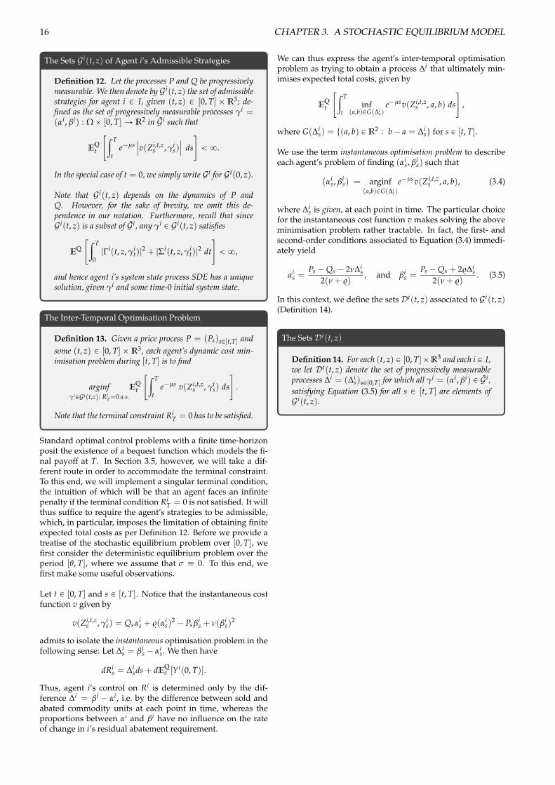
16 CHAPTER 3. A STOCHASTIC EQUILIBRIUM MODEL
The Sets G i(t, z) of Agent i’s Admissible Strategies
Definition 12. Let the processes P and Q be progressivelymeasurable. We then denote by G i(t, z) the set of admissiblestrategies for agent i P I, given (t, z) P [0, T] ˆ R3; de-fined as the set of progressively measurable processes g
i =(ai, b
i) : W ˆ [0, T] Ñ R2 in G i such that
EQt
"ª T
te´µs
ˇˇv(Zi,t,z
s , g
is)
ˇˇ ds
#† 8.
In the special case of t = 0, we simply write G i for G i(0, z).
Note that G i(t, z) depends on the dynamics of P andQ. However, for the sake of brevity, we omit this de-pendence in our notation. Furthermore, recall that sinceG i(t, z) is a subset of G i , any g
i P G i(t, z) satisfies
EQ
"ª T
0|Gi(t, z, g
it)|2 + |Si(t, z, g
it)|2 dt
#† 8,
and hence agent i’s system state process SDE has a uniquesolution, given g
i and some time-0 initial system state.
The Inter-Temporal Optimisation Problem
Definition 13. Given a price process P = (Ps)sP[t,T] andsome (t, z) P [0, T] ˆ R3, each agent’s dynamic cost min-imisation problem during [t, T] is to find
arginfg
iPG i(t,z): Ri
T=0 a.s.EQ
t
"ª T
te´µs v(Zi,t,z
s , g
is) ds
#.
Note that the terminal constraint RiT = 0 has to be satisfied.
Standard optimal control problems with a finite time-horizonposit the existence of a bequest function which models the fi-nal payoff at T. In Section 3.5, however, we will take a dif-ferent route in order to accommodate the terminal constraint.To this end, we will implement a singular terminal condition,the intuition of which will be that an agent faces an infinitepenalty if the terminal condition Ri
T = 0 is not satisfied. It willthus suffice to require the agent’s strategies to be admissible,which, in particular, imposes the limitation of obtaining finiteexpected total costs as per Definition 12. Before we provide atreatise of the stochastic equilibrium problem over [0, T], wefirst consider the deterministic equilibrium problem over theperiod [q, T], where we assume that s ” 0. To this end, wefirst make some useful observations.
Let t P [0, T] and s P [t, T]. Notice that the instantaneous costfunction v given by
v(Zi,t,zs , g
is) = Qsa
is + $(ai
s)2 ´ Psb
is + n(b
is)
2
admits to isolate the instantaneous optimisation problem in thefollowing sense: Let Di
s = b
is ´ a
is. We then have
dRis = Di
sds + dEQs [Yi(0, T)].
Thus, agent i’s control on Ri is determined only by the dif-ference Di = b
i ´ a
i, i.e. by the difference between sold andabated commodity units at each point in time, whereas theproportions between a
i and b
i have no influence on the rateof change in i’s residual abatement requirement.
We can thus express the agent’s inter-temporal optimisationproblem as trying to obtain a process Di that ultimately min-imises expected total costs, given by
EQt
"ª T
tinf
(a,b)PG(Dis)
e´µsv(Zi,t,zs , a, b) ds
#,
where G(Dis) = t(a, b) P R2 : b ´ a = Di
su for s P [t, T].
We use the term instantaneous optimisation problem to describeeach agent’s problem of finding (ai
s, b
is) such that
(ais, b
is) = arginf
(a,b)PG(Dis)
e´µsv(Zi,t,zs , a, b), (3.4)
where Dis is given, at each point in time. The particular choice
for the instantaneous cost function v makes solving the aboveminimisation problem rather tractable. In fact, the first- andsecond-order conditions associated to Equation (3.4) immedi-ately yield
a
is =
Ps ´ Qs ´ 2nDis
2(n + $), and b
is =
Ps ´ Qs + 2$Dis
2(n + $). (3.5)
In this context, we define the sets Di(t, z) associated to G i(t, z)(Definition 14).
The Sets Di(t, z)
Definition 14. For each (t, z) P [0, T]ˆ R3 and each i P I,we let Di(t, z) denote the set of progressively measurableprocesses Di = (Di
s)sP[0,T] for which all g
i = (ai, b
i) P G i ,satisfying Equation (3.5) for all s P [t, T] are elements ofG i(t, z).
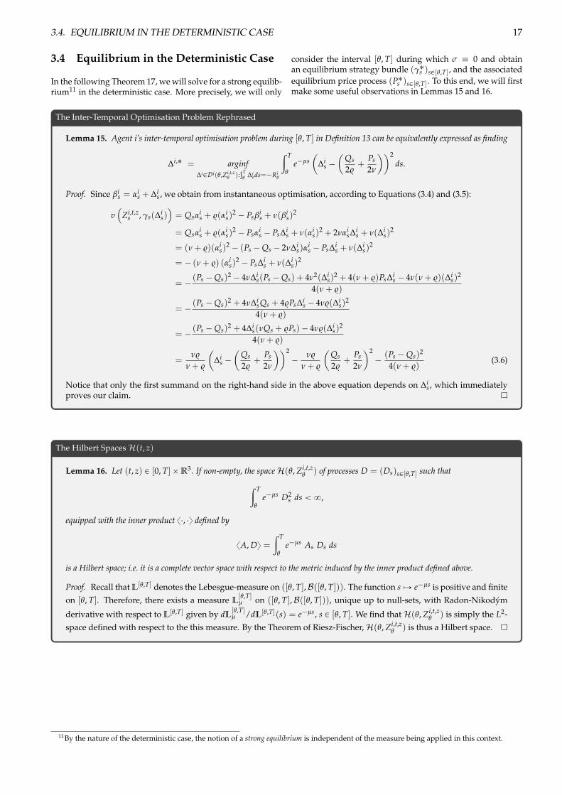
3.4. EQUILIBRIUM IN THE DETERMINISTIC CASE 17
3.4 Equilibrium in the Deterministic Case
In the following Theorem 17, we will solve for a strong equilib-rium11 in the deterministic case. More precisely, we will only
consider the interval [q, T] during which s ” 0 and obtainan equilibrium strategy bundle (g˚
s )sP[q,T], and the associatedequilibrium price process (P˚
s )sP[q,T]. To this end, we will firstmake some useful observations in Lemmas 15 and 16.
The Inter-Temporal Optimisation Problem Rephrased
Lemma 15. Agent i’s inter-temporal optimisation problem during [q, T] in Definition 13 can be equivalently expressed as finding
Di,˚ = arginfDi
PDi(q,Zi,t,zq
):≥T
q
Disds=´Ri
q
ª T
q
e´µs✓
Dis ´✓
Qs2$
+Ps2n
◆◆2ds.
Proof. Since b
is = a
is + Di
s, we obtain from instantaneous optimisation, according to Equations (3.4) and (3.5):
v⇣
Zi,t,zs , gs(Di
s)⌘= Qsa
is + $(ai
s)2 ´ Psb
is + n(b
is)
2
= Qsa
is + $(ai
s)2 ´ Psa
is ´ PsDi
s + n(ais)
2 + 2na
isDi
s + n(Dis)
2
= (n + $)(ais)
2 ´ (Ps ´ Qs ´ 2nDis)a
is ´ PsDi
s + n(Dis)
2
= ´ (n + $) (ais)
2 ´ PsDis + n(Di
s)2
= ´ (Ps ´ Qs)2 ´ 4nDis(Ps ´ Qs) + 4n
2(Dis)
2 + 4(n + $)PsDis ´ 4n(n + $)(Di
s)2
4(n + $)
= ´ (Ps ´ Qs)2 + 4nDisQs + 4$PsDi
s ´ 4n$(Dis)
2
4(n + $)
= ´ (Ps ´ Qs)2 + 4Dis(nQs + $Ps) ´ 4n$(Di
s)2
4(n + $)
=n$
n + $
✓Di
s ´✓
Qs2$
+Ps2n
◆◆2´ n$
n + $
✓Qs2$
+Ps2n
◆2´ (Ps ´ Qs)2
4(n + $)(3.6)
Notice that only the first summand on the right-hand side in the above equation depends on Dis, which immediately
proves our claim.
The Hilbert Spaces H(t, z)
Lemma 16. Let (t, z) P [0, T] ˆ R3. If non-empty, the space H(q, Zi,t,zq
) of processes D = (Ds)sP[q,T] such that
ª T
q
e´µs D2s ds † 8,
equipped with the inner product x¨, ¨y defined by
xA, Dy =ª T
q
e´µs As Ds ds
is a Hilbert space; i.e. it is a complete vector space with respect to the metric induced by the inner product defined above.
Proof. Recall that L[q,T] denotes the Lebesgue-measure on ([q, T],B([q, T])). The function s fiÑ e´µs is positive and finiteon [q, T]. Therefore, there exists a measure L
[q,T]µ
on ([q, T],B([q, T])), unique up to null-sets, with Radon-Nikodym
derivative with respect to L[q,T] given by dL[q,T]µ
/dL[q,T](s) = e´µs, s P [q, T]. We find that H(q, Zi,t,zq
) is simply the L2-space defined with respect to the this measure. By the Theorem of Riesz-Fischer, H(q, Zi,t,z
q
) is thus a Hilbert space.
11By the nature of the deterministic case, the notion of a strong equilibrium is independent of the measure being applied in this context.
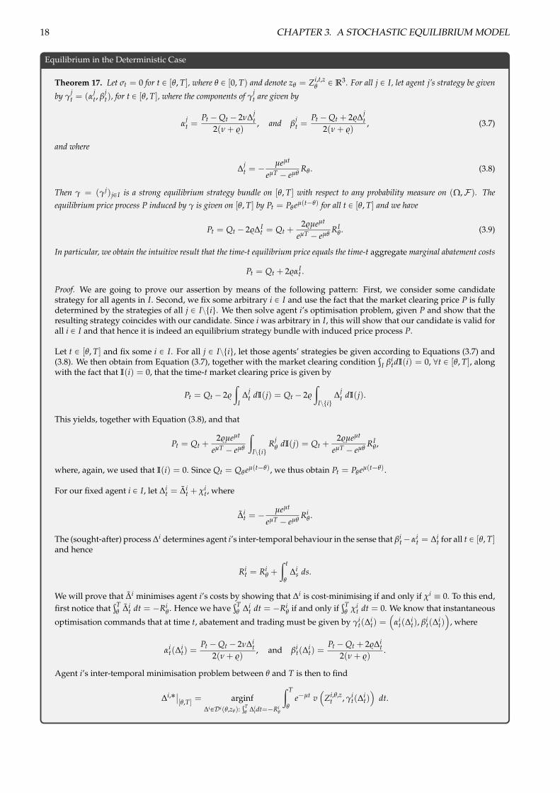
18 CHAPTER 3. A STOCHASTIC EQUILIBRIUM MODEL
Equilibrium in the Deterministic Case
Theorem 17. Let st = 0 for t P [q, T], where q P [0, T) and denote zq
= Zi,t,zq
P R3. For all j P I, let agent j’s strategy be givenby g
jt = (a
jt, b
jt), for t P [q, T], where the components of g
jt are given by
a
jt =
Pt ´ Qt ´ 2nDjt
2(n + $), and b
jt =
Pt ´ Qt + 2$Djt
2(n + $), (3.7)
and where
Djt = ´ µeµt
eµT ´ eµq
Rq
. (3.8)
Then g = (gj)jPI is a strong equilibrium strategy bundle on [q, T] with respect to any probability measure on (W,F ). Theequilibrium price process P induced by g is given on [q, T] by Pt = P
q
eµ(t´q) for all t P [q, T] and we have
Pt = Qt ´ 2$DIt = Qt +
2$µeµt
eµT ´ eµq
RIq
. (3.9)
In particular, we obtain the intuitive result that the time-t equilibrium price equals the time-t aggregate marginal abatement costs
Pt = Qt + 2$a
It .
Proof. We are going to prove our assertion by means of the following pattern: First, we consider some candidatestrategy for all agents in I. Second, we fix some arbitrary i P I and use the fact that the market clearing price P is fullydetermined by the strategies of all j P Iztiu. We then solve agent i’s optimisation problem, given P and show that theresulting strategy coincides with our candidate. Since i was arbitrary in I, this will show that our candidate is valid forall i P I and that hence it is indeed an equilibrium strategy bundle with induced price process P.
Let t P [q, T] and fix some i P I. For all j P Iztiu, let those agents’ strategies be given according to Equations (3.7) and(3.8). We then obtain from Equation (3.7), together with the market clearing condition
≥I b
itdI(i) = 0, @t P [q, T], along
with the fact that I(i) = 0, that the time-t market clearing price is given by
Pt = Qt ´ 2$
ª
IDj
t dI(j) = Qt ´ 2$
ª
IztiuDj
t dI(j).
This yields, together with Equation (3.8), and that
Pt = Qt +2$µeµt
eµT ´ eµq
ª
IztiuRj
q
dI(j) = Qt +2$µeµt
eµT ´ eµq
RIq
,
where, again, we used that I(i) = 0. Since Qt = Qq
eµ(t´q), we thus obtain Pt = Pq
eµ(t´q).
For our fixed agent i P I, let Dit = Di
t + c
it, where
Dit = ´ µeµt
eµT ´ eµq
Riq
.
The (sought-after) process Di determines agent i’s inter-temporal behaviour in the sense that b
it ´ a
it = Di
t for all t P [q, T]and hence
Rit = Ri
q
+ª t
q
Dis ds.
We will prove that Di minimises agent i’s costs by showing that Di is cost-minimising if and only if c
i ” 0. To this end,first notice that
≥Tq
Dit dt = ´Ri
q
. Hence we have≥T
q
Dit dt = ´Ri
q
if and only if≥T
q
c
it dt = 0. We know that instantaneous
optimisation commands that at time t, abatement and trading must be given by g
it(D
it) =
⇣a
it(D
it), b
it(D
it)⌘
, where
a
it(D
it) =
Pt ´ Qt ´ 2nDit
2(n + $), and b
it(D
it) =
Pt ´ Qt + 2$Dit
2(n + $).
Agent i’s inter-temporal minimisation problem between q and T is then to find
Di,˚ ˇ[q,T] = arginf
DiPDi(q,z
q
):≥T
q
Ditdt=´Ri
q
ª T
q
e´µt v⇣
Zi,q,zt , g
it(D
it)⌘
dt.
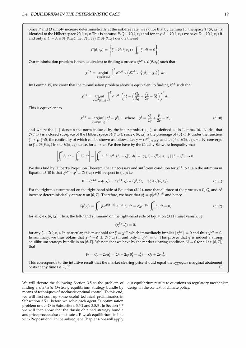
3.4. EQUILIBRIUM IN THE DETERMINISTIC CASE 19
Since P and Q simply increase deterministically at the risk-free rate, we notice that by Lemma 15, the space Di(q, zq
) isidentical to the Hilbert space H(q, z
q
): This is because P, Q P H(q, zq
) and for any A P H(q, zq
) we have D P H(q, zq
) ifand only if D ´ A P H(q, z
q
). Let C(q, zq
) Ñ H(q, zq
) denote the set
C(q, zq
) =
#z P H(q, z
q
) :ª T
q
zt dt = 0
+.
Our minimisation problem is then equivalent to finding a process c
i,˚ P C(q, zq
) such that
c
i,˚ = arginfc
iPC(q,z
q
)
ª T
te´µt v
⇣Zi,q,z
t , g
it(D
it + c
it)⌘
dt.
By Lemma 15, we know that the minimisation problem above is equivalent to finding c
i,˚ such that
c
i,˚ = arginfc
iPC(q,z
q
)
ª T
q
e´µt✓
c
it ´✓
Qt2$
+Pt2n
´ Dit
◆◆2dt.
This is equivalent to
c
i,˚ = arginfc
iPC(q,z
q
)}c
i ´ f
i}, where f
i =Q2$
+P2n
´ Di, (3.10)
and where the } ¨ } denotes the norm induced by the inner product x¨, ¨y, as defined as in Lemma 16. Notice thatC(q, z
q
) is a closed subspace of the Hilbert space H(q, zq
), since C(q, zq
) is the preimage of t0u Ä R under the functionz fiÑ ≥T
q
ztdt, the continuity of which can be shown as follows: Let h = (eµt)tP[q,T] and let z
n P H(q, zq
), n P N, convergeto z P H(q, z
q
) in the H(q, zq
)-sense, for n Ñ 8. We then have by the Cauchy-Schwarz Inequality thatˇˇˇ
ª T
q
zt dt ´ª T
q
z
nt dt
ˇˇˇ =
ˇˇˇ
ª T
q
e´µt eµt (zt ´ z
nt ) dt
ˇˇˇ = |xh, z ´ z
ny| § }h} }z ´ z
n} Ñ 0.
We thus find by Hilbert’s Projection Theorem, that a necessary and sufficient condition for c
i,˚ to attain the infimum inEquation 3.10 is that c
i,˚ ´ f
i K C(q, zq
) with respect to x¨, ¨y; i.e.
0 = xc
i,˚ ´ f
i, zy = xc
i,˚, zy ´ xf
i, zy, @z P C(q, zq
). (3.11)
For the rightmost summand on the right-hand side of Equation (3.11), note that all three of the processes P, Q, and Di
increase deterministically at rate µ on [q, T]. Therefore, we have that f
it = f
iq
eµ(t´q) and hence
xf
i, zy =ª T
q
f
q
eµ(t´q) e´µtzt dt = f
iq
e´µq
ª T
q
zt dt = 0, (3.12)
for all z P C(q, zq
). Thus, the left-hand summand on the right-hand side of Equation (3.11) must vanish; i.e.
xc
i,˚, zy = 0,
for any z P C(q, zq
). In particular, this must hold for z = c
i,˚ which immediately implies }c
i,˚} = 0 and thus c
i,˚ ” 0.In summary, we thus obtain that c
i,˚ ´ f K C(q, zq
) if and only if c
i,˚ ” 0. This proves that g is indeed a strongequilibrium strategy bundle in on [q, T]. We note that we have by the market clearing condition b
It = 0 for all t P [q, T],
that
Pt = Qt ´ 2$Djt = Qt ´ 2$(b
It ´ a
It ) = Qt + 2$a
It .
This corresponds to the intuitive result that the market clearing price should equal the aggregate marginal abatementcosts at any time t P [q, T].
We will devote the following Section 3.5 to the problem offinding a stochastic Q-strong equilibrium strategy bundle bymeans of techniques of stochastic optimal control. To this end,we will first sum up some useful technical preliminaries inSubsection 3.5.1, before we solve each agent i’s optimisationproblem under Q in Subsections 3.5.2 and 3.5.3 . In Section 3.7we will then show that the thusly obtained strategy bundleand price process also constitute a P-weak equilibrium, in linewith Proposition 7. In the subsequent Chapter 4, we will apply
our equilibrium results to questions on regulatory mechanismdesign in the context of climate policy.
20 CHAPTER 3. A STOCHASTIC EQUILIBRIUM MODEL
3.5 Strong Equilibrium under a Risk-Neutral Measure
We will now derive a strong equilibrium with respect to themeasure Q. In Subsection 3.7 we will then use the equilibriumdynamics obtained in the following, to present sufficient con-ditions under which Q „ P and hence the Q-strong equilib-rium is also a weak equilibrium under the objective measureP. In order to solve each agent’s optimisation problem, wewill first introduce some useful technical preliminaries fromthe theory of optimal stochastic control.
3.5.1 Technical Preliminaries: OptimalStochastic Control
Our treatise of technical preliminaries in this Subsection 3.5.1follows the presentation in [Pham, 2009], Chapter 3, the no-tation in which we amend to fit our purposes and which weaugment with explanatory details and economic intuition. Wefirst define the key notions necessary for our treatise. Foreach agent i, these are the cost function (Definition 18), whichsimply captures the expected future costs induced by a givenstrategy; and the associated value function (Definition 19)which captures how the infimum of future expected costs re-sponds to instantaneous changes in the agent’s state process.
Agent i’s Cost Functional
Definition 18. We define the agents’ cost functional J : [0, T] ˆ R3 ˆ R2 by
J(t, z, g
i) = EQt
"ª T
te´µs v(Zi,t,z
s , g
is) ds
#,
for all (t, z) P [0, T] ˆ R3 and all g
i P G i(t, z).
Agent i’s Value Function
Definition 19. We define the value function associated to each agent i’s optimisation problem by
wi,˚(t, z) = infg
iPG i(t,z)
J(t, z, g
i).
for all (t, z) P [0, T] ˆ R3.
The Dynamic Programming Principle In the followingwe will lay out ready a useful set of tools that we will use tosolve the problem of optimal stochastic control for each agent.Namely, these are the dynamic programming principle (DPP)and the Hamilton-Jacobi-Bellman (HJB) equation. Similar to
the discrete-time case, the solutions to continuous-time opti-mal stochastic control problems can often be found based onthe following Theorem 20 (cf. [Pham, 2009], Remark 3.3.3.), aproof of which we will provide further below
The Dynamic Programming Principle (DPP)
Theorem 20. Let t P [0, T]. For all g
i P G i(t, z) and all stopping times t P [t, T] we have
wi,˚(t, z) § EQt
ªt
te´µsv(Zi,t,z
s , g
i) ds + wi,˚(t, Zi,t,zt
)
�. (3.13)
Furthermore, for all e ° 0, there exists a strategy g
i P G i(t, z) such that for all stopping times t P [t, T] we have
wi,˚(t, z) + e • EQt
ªt
te´µsv(Zi,t,z
s , g
i) ds + wi,˚(t, Zi,t,zt
)
�. (3.14)
The natural interpretation of Equations (3.13) and (3.14) is thatthe optimisation can be ‘split in two’ with respect to the time-dimension at any random point t P [t, T]. That is, in analogyto dynamic programming in discrete time, where we can startthe optimisation at T using some terminal condition, and thenwork our way back towards t = 0, either algorithmically or inclosed-form, here we have a similar formulation in continuoustime: Once we know the optimal outcome over the remaining
timeframe [t, T] (i.e. wi,˚(t, Zi,t,zt
)), we have that, on the onehand, any control implemented over [t, t] will at best yield theoptimal outcome over the entire period (Equation (3.13)). Onthe other hand, such strategies can come arbitrarily close tothat optimal outcome (Equation (3.14)). Note that we have anequivalent formulation in the form of the following Corollary21 (cf. [Pham, 2009], Theorem 3.3.1).
3.5. STRONG EQUILIBRIUM UNDER A RISK-NEUTRAL MEASURE 21
Alternative Formulation of the DPP
Corollary 21. For (t, z) P [0, T] ˆ R3 we have
wi,˚(t, z) = infg
iPG i(t,z)
suptP[t,T]
EQt
ªt
te´µsv(Zi,t,z
s , g
is) ds + wi,˚(t, Zi,t,z
t
)
�
= infg
iPG i(t,z)
inftP[t,T]
EQt
ªt
te´µsv(Zi,t,z
s , g
is) ds + wi,˚(t, Zi,t,z
t
)
�. (3.15)
Even though the formulation in Corollary 21 is somewhatmore compact, the form presented in Theorem 20 is quite use-ful for the derivation of the Hamilton-Jacobi-Bellman equationas we shall see in the following. In the interest of complete-
ness, we will first provide a proof of Theorem 20, which, as aby-product yields a proof of Corollary 21, and the formulationprovided in Equation (3.15).
Proof of Theorem 20
Proof of Theorem 20. (i) We first prove Equation (3.13). We fix a control g
i P G i(t, z). The solution to the dynamics
dZit = Gi(t, Zi
t, g
it)dt + Si(t, Zi
t, g
it)dWQ
t (3.16)
with fixed initial value Zi0 is pathwise unique; i.e. any two of its solutions, Z and Z satisfy Q[Zs = Zs : s P
[0, T]] = 1. This implies that for any stopping time t P [t, T] we have
Zi,t,zs = Zi,t,Zi,t,z
t
s : s P [t, T].
That is, if we consider the solution (Zi,t,zs )sP[t,T] to the SDE (3.16) over [t, T] starting at z, and observe its value at
time t, i.e. Zi,t,zt
, then the process solving (3.16) over [t, T] with fixed initial value Zi,t,zt
at time t, is (a.s.) pathwiseidentical to the original solution (Zi,t,z
s )sP[t,T]. This Markovian structure yields by the law of iterated conditionalexpectation (‘tower property’) that
J(t, z, g
is) = EQ
t
"ª T
te´µsv(Zi,t,z
s , g
is) ds
#
= EQt
"ªt
te´µsv(Zi,t,z
s , g
is) ds +
ª T
t
e´µsv(Zi,t,zs , g
is) ds
#
= EQt
"ªt
te´µsv(Zi,t,z
s , g
is) ds + EQ
t
"ª T
t
e´µsv(Zi,t,zs , g
is) ds
##
= EQt
ªt
te´µsv(Zi,t,z
s , g
is) ds + J(t, Zi,t,z
t
, g
is)
�.
Since by definition of wi,˚ we have J(t, z, g
i) • wi,˚(t, z) for all t, z P [0, T] ˆ R3 and since t is arbitrary in [t, T] itfollows that
J(t, z, g
i) § suptP[t,T]
EQt
ªt
te´µsv(Zi,t,z
s , g
i) ds + wi,˚(t, Zi,t,zt
)
�
Taking the infimum over all admissible controls g
i P G i(t, z) on the left-hand side of the above inequality, weobtain
wi,˚(t, z) § infg
iPG i(t,z)
EQt
ªt
te´µsv(Zi,t,z
s , g
i) ds + wi,˚(t, Zi,t,zt
)
�,
which is the desired Equation (3.13).(ii) We now want to prove Equation (3.14). To this end we fix some arbitrary control g
i P G i(t, z) and some arbitrarystopping time t P [t, T]. By definition, wi,˚ is the infimum of the cost functional over the set of admissible controls.Hence for any deviation e ° 0 from that infimum and any w P W, there must exists a control g
i,e which improvesupon that deviation in the sense that
J⇣
t, Zi,t,zt
, g
i,e⌘
§ wi,˚⇣
t, Zi,t,zt
⌘+ e. (3.17)
We now define the process g
i by
g
is(w) =
#g
is(w) : 0 § s § t(w)
g
i,e,ws (w) : t(w) § s § T
for s P [t, T], w P W.
22 CHAPTER 3. A STOCHASTIC EQUILIBRIUM MODEL
The process g
i can be shown to be progressively measurable (see [Bertsekas and Shreve, 1978], Chapter 7) andthus is an element of G i(t, z). From Equation (3.17), and by the law of iterated conditional expectation we obtain
EQt
ªt
te´µs v(Zi,t,z
s , g
is) ds + wi,˚(t, Zi,t,z
t
)
�§EQ
t
ªt
te´µs v(Zi,t,z
s , g
is) ds + J(t, Zi,t,z
t
, g
i,e)
�
§EQt
ªt
te´µs v(Zi,t,z
s , g
is) ds + wi,˚(t, Zi,t,z
t
)
�+ e
Since g
i P G i(t, z) and t P [t, T] are arbitrary (in particular during [t, t]), we obtain the desired inequality (3.14),as well as Corollary 21.
Note that the statement in Theorem 20 and the equivalent for-mulation provided by Equation 3.15 is a stronger formulationof the statement that wi,˚(t, z) equals the expression
infgPG i(t,z)
EQt
ªt
te´µsv(s, Zi,t,z
s , g
i) ds + wi,˚(t, Zi,t,zt
)
�, (3.18)
for all stopping times t P [t, T], which is a common formula-tion of the Dynamic Programming Principle.
The Hamilton-Jacobi-Bellman Equation The DynamicProgramming Principle can be used to examine the local be-haviour of the value function at t+ for any time t P [0, T]:More precisely, by letting the stopping time t converge to t,we can examine the increment in wi,˚ for an infinitesimallysmall increment in time. We will use the DPP in the formof Equations (3.13) and (3.14) in order to formally derive theso-called Hamilton-Jacobi-Bellman (HJB) partial differential
equation, which characterises the local behaviour of the valuefunction at t+. As is customary, we will later use the HJB equa-tion to find a closed-form representation of the value function(by solving the HJB Equation associated to our equilibriumproblem explicitly) and, as a by-product, obtain an optimalstochastic control g
i,˚ for agent i. In the following, will heuris-tically derive that the value function should satisfy what iscalled the Hamilton-Jacobi-Bellman differential equation, whichis a partial differential equation of the form
0 = Dtw(t, z) + L(a,b)w(t, z) + e´µsv(s, z, a, b),
where w denotes a sufficiently smooth function. The func-tional L(a,b) will be specified in the following.
Note that throughout the text, we use the notation Dz, to de-note the differential operator with respect to z, and accord-ingly for other parameters.
Heuristic Derivation of the Hamilton-Jacobi-Bellman Equation
(1) We will first use Equation (3.13) to show that wi,˚ should satisfy a condition of the form
0 § Dtwi,˚(t, z) + L(a,b)wi,˚(t, z) + e´µsv(s, z, a, b).
To this end, consider some stopping time t valued in [t, T], and a constant control g
i ” (a, b) P R2. We then have byEquation (3.13) of the DPP:
wi,˚(t, z) § EQt
ªt
te´µsv(Zi,t,z
s , g
is) ds + wi,˚(t, Zi,t,z
t
)
�. (3.19)
If wi,˚ is smooth enough, i.e. if wi,˚ : [0, T]ˆ R3 Ñ R is at least once continuously differentiable in the first and at leasttwice continuously differentiable in the second argument, we can apply Ito’s Lemma (in integral form). Recalling thatG and S denote the drift and volatility term in the dynamics of Zi we obtain
wi,˚(t, Zi,t,zt
) = wi,˚(t, z) +ª
t
t
⇣Dtwi,˚ + L(a,b)
⌘(s, Zi,t,z
s ) ds + x
t
, (3.20)
where x is a local martingale starting in zero at time t and where L(a,b) is the infinitesimal generator associated to (a, b)and the dynamics dZi of Zi, defined as
L(a,b)wi,˚ = G(t, z, a, b).Dzwi,˚ +12
tr(S(t, z, a, b)S1(t, z, a, b)D2z wi,˚).
Here, the period operator ‘.’ denotes the vector product on R3, tr(¨) denotes the trace operator on the space of 3 ˆ 3-matrices and S1 denotes the transposition of S. The infinitesimal generator L(a,b) associated to (a, b) and dZi has astraightforward economic interpretation: First, consider the left-hand component G(t, z, a, b).Dzwi,˚. Here, the linearapproximation to z at the point (t, z) is scaled in each dimension by the drift component in the dynamics of Zi. Ac-cordingly, G(t, z, a, b).Dzwi,˚ is the linear approximation of the drift in the dynamics dwi,˚ of wi,˚. This, together withDtwi,˚ in Equation (3.20) forms the component referring to the deterministic derivative in Equation (3.20). The right-hand component of L(a,b)wi,˚, on the other hand, captures the effect of random perturbations during [t, q] on i’s valuefunction: Here, the quadratic approximation is scaled in each dimension with the respective element in the ‘covariance
3.5. STRONG EQUILIBRIUM UNDER A RISK-NEUTRAL MEASURE 23
matrix’ S(t, z, a, b).Equations (3.19) and (3.20) together yield
0 = wi,˚(t, z) ´ EQt [w
i,˚(t, z)]
=wi,˚(t, z) ´ EQt
wi,˚(t, Zi,t,z
t
) ´ª
t
t(Dtwi,˚ + L(a,b))(s, Zi,t,z
s ) ds + x
t
�
§EQt
ªt
te´µsv(s, Zi,t,z
s , g
is) ds + wi,˚(t, Zi,t,z
t
) ´ wi,˚(t, Zi,t,zt
) +ª
t
t(Dtwi,˚ + L(a,b))(s, Zi,t,z
s ) ds + x
t
�
=EQt
ªt
t
⇣Dtwi,˚ + L(a,b)wi,˚
⌘(s, Zi,t,z
s ) + e´µsv(Zi,t,zs , a, b) ds + x
t
�.
In order to get rid of the expectation EQt [xt
], we recall that since x is a local martingale, there exists a sequence (tn)nPN
of stopping times such that limnÑ8
tn = 8 a.s. and the stopped process x
tn is a martingale for all n P N. Lettn = (t + 1
n ) ^ tn. Then limnÑ8
tn = t and the stopped process x
tn is a martingale for all n and thus has vanishingtime-t conditional expectation. Hence we obtain
0 § EQt
ªtn
t
⇣Dtwi,˚ + L(a,b)wi,˚
⌘(s, Zi,t,z
s ) + e´µsv(Zi,t,zs , a, b) ds
�.
We want to transfer this inequality to the integrand on the right-hand side. To this end, first notice that the aboveinequality implies by the smoothness we posited that
0 § limnÑ8
EQt
1tn
ªtn
t
⇣Dtwi,˚ + L(a,b)wi,˚
⌘(s, Zi,t,z
s ) + e´µsv(Zi,t,zs , a, b) ds
�(3.21)
= Dtwi,˚(t, z) + L(a,b)wi,˚(t, z) + e´µsv(s, z, a, b). (3.22)
(2) In order to formally derive equality in Equation (3.21), let g
i,˚ be an optimal control for agent i. Then by (3.18) wehave for all n P N that
wi,˚ = EQt
ªtn
te´µs v(Zi,˚
s , g
i,˚s ) ds + wi,˚(tn, Zi,˚
tn )
�,
where Zi,˚ is the solution to the SDE governing the system dynamics starting from z at time t with control g
i,˚.By proceeding similarly as above, we obtain
Dtwi,˚(t, z) + Lg
i,˚t wi,˚(t, z) + e´µsv(s, z, g
i,˚t ) = 0.
This, together with Equation (3.22) suggests that wi,˚ should satisfy the partial differential equation
0 = Dtwi,˚(t, z) + infaPG
hL(a,b)wi,˚(t, z) + e´µtv(t, z, a, b)
i,
for all (t, z) P [0, T) ˆ R3, if the infimum is finite. 4
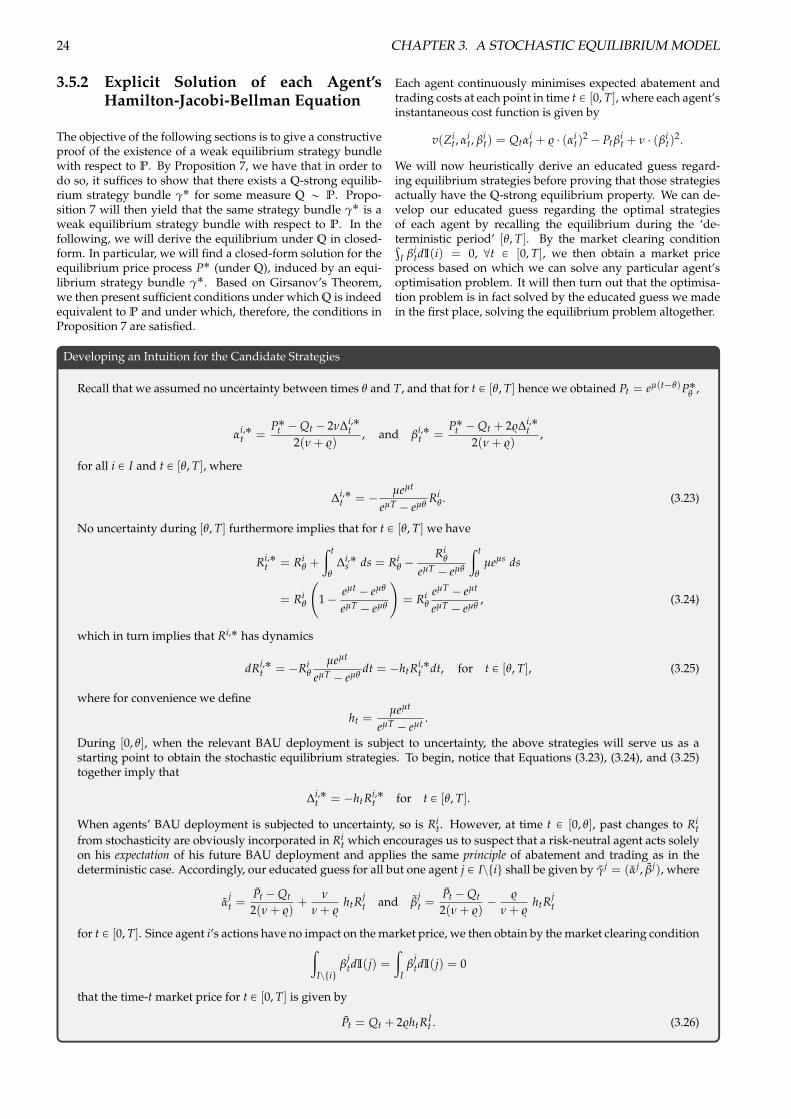
24 CHAPTER 3. A STOCHASTIC EQUILIBRIUM MODEL
3.5.2 Explicit Solution of each Agent’sHamilton-Jacobi-Bellman Equation
The objective of the following sections is to give a constructiveproof of the existence of a weak equilibrium strategy bundlewith respect to P. By Proposition 7, we have that in order todo so, it suffices to show that there exists a Q-strong equilib-rium strategy bundle g
˚ for some measure Q „ P. Propo-sition 7 will then yield that the same strategy bundle g
˚ is aweak equilibrium strategy bundle with respect to P. In thefollowing, we will derive the equilibrium under Q in closed-form. In particular, we will find a closed-form solution for theequilibrium price process P˚ (under Q), induced by an equi-librium strategy bundle g
˚. Based on Girsanov’s Theorem,we then present sufficient conditions under which Q is indeedequivalent to P and under which, therefore, the conditions inProposition 7 are satisfied.
Each agent continuously minimises expected abatement andtrading costs at each point in time t P [0, T], where each agent’sinstantaneous cost function is given by
v(Zit, a
it, b
it) = Qta
it + $ ¨ (ai
t)2 ´ Ptb
it + n ¨ (b
it)
2.
We will now heuristically derive an educated guess regard-ing equilibrium strategies before proving that those strategiesactually have the Q-strong equilibrium property. We can de-velop our educated guess regarding the optimal strategiesof each agent by recalling the equilibrium during the ‘de-terministic period’ [q, T]. By the market clearing condition≥
I b
itdI(i) = 0, @t P [0, T], we then obtain a market price
process based on which we can solve any particular agent’soptimisation problem. It will then turn out that the optimisa-tion problem is in fact solved by the educated guess we madein the first place, solving the equilibrium problem altogether.
Developing an Intuition for the Candidate Strategies
Recall that we assumed no uncertainty between times q and T, and that for t P [q, T] hence we obtained Pt = eµ(t´q)P˚
q
,
a
i,˚t =
P˚
t ´ Qt ´ 2nDi,˚t
2(n + $), and b
i,˚t =
P˚
t ´ Qt + 2$Di,˚t
2(n + $),
for all i P I and t P [q, T], where
Di,˚t = ´ µeµt
eµT ´ eµq
Riq
. (3.23)
No uncertainty during [q, T] furthermore implies that for t P [q, T] we have
Ri,˚t = Ri
q
+ª t
q
Di,˚s ds = Ri
q
´ Riq
eµT ´ eµq
ª t
q
µeµs ds
= Riq
1 ´ eµt ´ eµq
eµT ´ eµq
!= Ri
q
eµT ´ eµt
eµT ´ eµq
, (3.24)
which in turn implies that Ri,˚ has dynamics
dRi,˚t = ´Ri
q
µeµt
eµT ´ eµq
dt = ´htRi,˚t dt, for t P [q, T], (3.25)
where for convenience we define
ht =µeµt
eµT ´ eµt .
During [0, q], when the relevant BAU deployment is subject to uncertainty, the above strategies will serve us as astarting point to obtain the stochastic equilibrium strategies. To begin, notice that Equations (3.23), (3.24), and (3.25)together imply that
Di,˚t = ´htRi,˚
t for t P [q, T].
When agents’ BAU deployment is subjected to uncertainty, so is Rit. However, at time t P [0, q], past changes to Ri
tfrom stochasticity are obviously incorporated in Ri
t which encourages us to suspect that a risk-neutral agent acts solelyon his expectation of his future BAU deployment and applies the same principle of abatement and trading as in thedeterministic case. Accordingly, our educated guess for all but one agent j P Iztiu shall be given by g
j = (aj, b
j), where
a
jt =
Pt ´ Qt2(n + $)
+n
n + $
htRjt and b
jt =
Pt ´ Qt2(n + $)
´ $
n + $
htRjt
for t P [0, T]. Since agent i’s actions have no impact on the market price, we then obtain by the market clearing conditionª
Iztiub
jtdI(j) =
ª
Ib
jtdI(j) = 0
that the time-t market price for t P [0, T] is given by
Pt = Qt + 2$htRIt . (3.26)
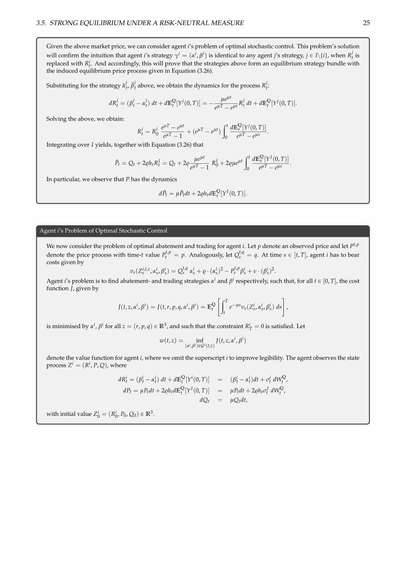
3.5. STRONG EQUILIBRIUM UNDER A RISK-NEUTRAL MEASURE 25
Given the above market price, we can consider agent i’s problem of optimal stochastic control. This problem’s solutionwill confirm the intuition that agent i’s strategy g
i = (ai, b
i) is identical to any agent j’s strategy, j P Iztiu, when Rjt is
replaced with Rit. And accordingly, this will prove that the strategies above form an equilibrium strategy bundle with
the induced equilibrium price process given in Equation (3.26).
Substituting for the strategy a
jt, b
jt above, we obtain the dynamics for the process Rj
t:
dRjt = (b
jt ´ a
jt) dt + dEQ
t [Yj(0, T)] = ´ µeµt
eµT ´ eµt Rjt dt + dEQ
t [Yj(0, T)].
Solving the above, we obtain:
Rjt = Rj
0eµT ´ eµt
eµT ´ 1+ (eµT ´ eµt)
ª t
0
dEQs [Yj(0, T)]eµT ´ eµs .
Integrating over I yields, together with Equation (3.26) that
Pt = Qt + 2$htRIt = Qt + 2$
µeµt
eµT ´ 1RI
0 + 2$µeµtª t
0
dEQs [YI(0, T)]eµT ´ eµs .
In particular, we observe that P has the dynamics
dPt = µPtdt + 2$htdEQt [Y
I(0, T)].
Agent i’s Problem of Optimal Stochastic Control
We now consider the problem of optimal abatement and trading for agent i. Let p denote an observed price and let Pt,p
denote the price process with time-t value Pt,pt = p. Analogously, let Qt,q
t = q. At time s P [t, T], agent i has to bearcosts given by
vs(Zi,t,zs , a
is, b
is) = Qt,q
s a
is + $ ¨ (ai
s)2 ´ Pt,p
s b
is + n ¨ (b
is)
2.
Agent i’s problem is to find abatement- and trading strategies a
i and b
i respectively, such that, for all t P [0, T], the costfunction J, given by
J(t, z, a
i, b
i) = J(t, r, p, q, a
i, b
i) = EQt
"ª T
te´µsvs(Zi
s, a
is, b
is) ds
#,
is minimised by a
i, b
i for all z = (r, p, q) P R3, and such that the constraint RiT = 0 is satisfied. Let
w(t, z) = inf(ai ,bi)PG i(t,z)
J(t, z, a
i, b
i)
denote the value function for agent i, where we omit the superscript i to improve legibility. The agent observes the stateprocess Zi = (Ri, P, Q), where
dRit = (b
it ´ a
it) dt + dEQ
t [Yi(0, T)] = (b
it ´ a
it)dt + s
it dWQ
t ,
dPt = µPtdt + 2$htdEQt [Y
I(0, T)] = µPtdt + 2$htsIt dWQ
t ,dQt = µQtdt,
with initial value Zi0 = (Ri
0, P0, Q0) P R3.
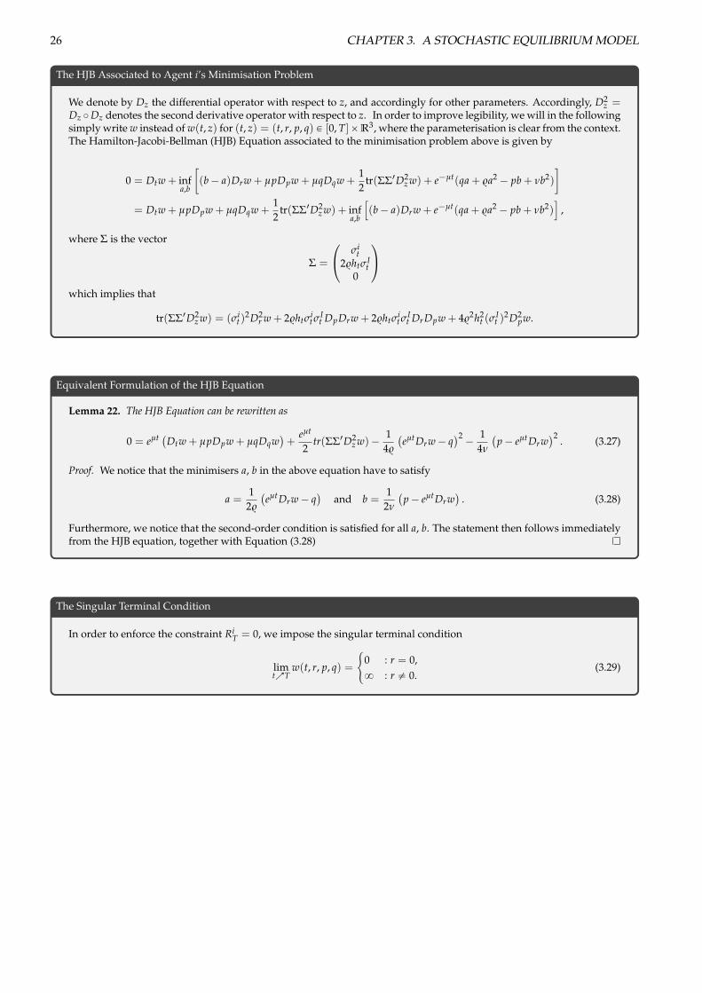
26 CHAPTER 3. A STOCHASTIC EQUILIBRIUM MODEL
The HJB Associated to Agent i’s Minimisation Problem
We denote by Dz the differential operator with respect to z, and accordingly for other parameters. Accordingly, D2z =
Dz ˝ Dz denotes the second derivative operator with respect to z. In order to improve legibility, we will in the followingsimply write w instead of w(t, z) for (t, z) = (t, r, p, q) P [0, T]ˆ R3, where the parameterisation is clear from the context.The Hamilton-Jacobi-Bellman (HJB) Equation associated to the minimisation problem above is given by
0 = Dtw + infa,b
(b ´ a)Drw + µpDpw + µqDqw +
12
tr(SS1D2z w) + e´µt(qa + $a2 ´ pb + nb2)
�
= Dtw + µpDpw + µqDqw +12
tr(SS1D2z w) + inf
a,b
h(b ´ a)Drw + e´µt(qa + $a2 ´ pb + nb2)
i,
where S is the vector
S =
0
@s
it
2$htsIt
0
1
A
which implies that
tr(SS1D2z w) = (si
t)2D2
r w + 2$htsit s
It DpDrw + 2$hts
it s
It DrDpw + 4$
2h2t (s
It )
2D2pw.
Equivalent Formulation of the HJB Equation
Lemma 22. The HJB Equation can be rewritten as
0 = eµt �Dtw + µpDpw + µqDqw�+
eµt
2tr(SS1D2
z w) ´ 14$
�eµtDrw ´ q
�2 ´ 14n
�p ´ eµtDrw
�2 . (3.27)
Proof. We notice that the minimisers a, b in the above equation have to satisfy
a =1
2$
�eµtDrw ´ q
�and b =
12n
�p ´ eµtDrw
�. (3.28)
Furthermore, we notice that the second-order condition is satisfied for all a, b. The statement then follows immediatelyfrom the HJB equation, together with Equation (3.28)
The Singular Terminal Condition
In order to enforce the constraint RiT = 0, we impose the singular terminal condition
limtÕT
w(t, r, p, q) =
#0 : r = 0,8 : r ‰ 0.
(3.29)
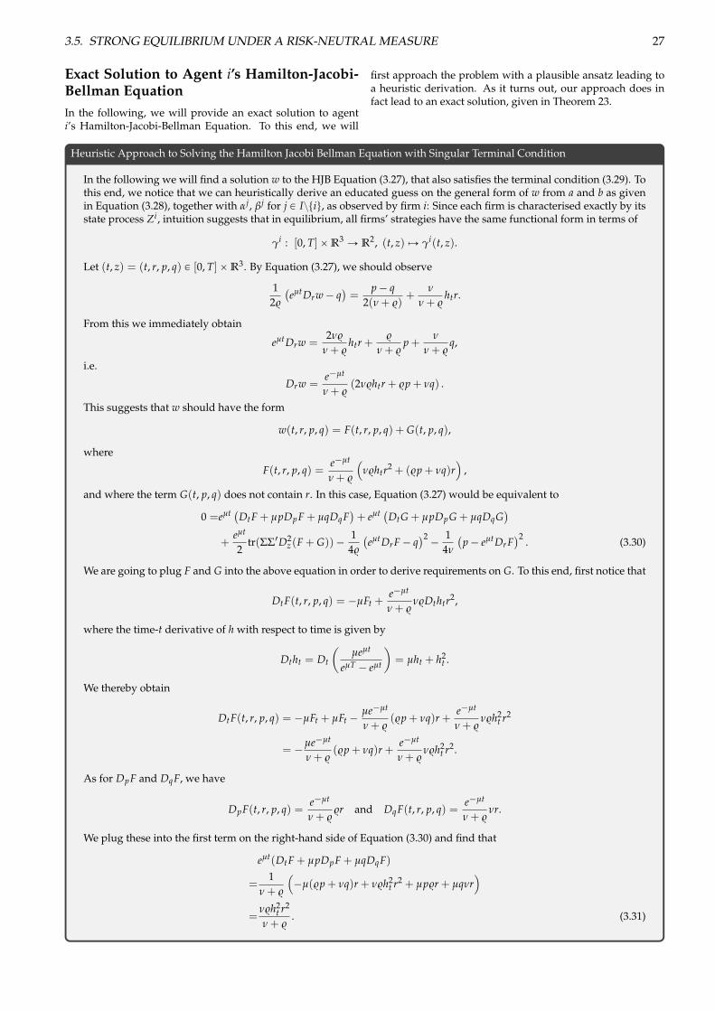
3.5. STRONG EQUILIBRIUM UNDER A RISK-NEUTRAL MEASURE 27
Exact Solution to Agent i’s Hamilton-Jacobi-Bellman EquationIn the following, we will provide an exact solution to agenti’s Hamilton-Jacobi-Bellman Equation. To this end, we will
first approach the problem with a plausible ansatz leading toa heuristic derivation. As it turns out, our approach does infact lead to an exact solution, given in Theorem 23.
Heuristic Approach to Solving the Hamilton Jacobi Bellman Equation with Singular Terminal Condition
In the following we will find a solution w to the HJB Equation (3.27), that also satisfies the terminal condition (3.29). Tothis end, we notice that we can heuristically derive an educated guess on the general form of w from a and b as givenin Equation (3.28), together with a
j, b
j for j P Iztiu, as observed by firm i: Since each firm is characterised exactly by itsstate process Zi, intuition suggests that in equilibrium, all firms’ strategies have the same functional form in terms of
g
i : [0, T] ˆ R3 Ñ R2, (t, z) fiÑ g
i(t, z).
Let (t, z) = (t, r, p, q) P [0, T] ˆ R3. By Equation (3.27), we should observe
12$
�eµtDrw ´ q
�=
p ´ q2(n + $)
+n
n + $
htr.
From this we immediately obtain
eµtDrw =2n$
n + $
htr +$
n + $
p +n
n + $
q,
i.e.
Drw =e´µt
n + $
(2n$htr + $p + nq) .
This suggests that w should have the form
w(t, r, p, q) = F(t, r, p, q) + G(t, p, q),
where
F(t, r, p, q) =e´µt
n + $
⇣n$htr2 + ($p + nq)r
⌘,
and where the term G(t, p, q) does not contain r. In this case, Equation (3.27) would be equivalent to
0 =eµt �DtF + µpDpF + µqDqF�+ eµt �DtG + µpDpG + µqDqG
�
+eµt
2tr(SS1D2
z (F + G)) ´ 14$
�eµtDrF ´ q
�2 ´ 14n
�p ´ eµtDrF
�2 . (3.30)
We are going to plug F and G into the above equation in order to derive requirements on G. To this end, first notice that
DtF(t, r, p, q) = ´µFt +e´µt
n + $
n$Dthtr2,
where the time-t derivative of h with respect to time is given by
Dtht = Dt
✓µeµt
eµT ´ eµt
◆= µht + h2
t .
We thereby obtain
DtF(t, r, p, q) = ´µFt + µFt ´ µe´µt
n + $
($p + nq)r +e´µt
n + $
n$h2t r2
= ´ µe´µt
n + $
($p + nq)r +e´µt
n + $
n$h2t r2.
As for DpF and DqF, we have
DpF(t, r, p, q) =e´µt
n + $
$r and DqF(t, r, p, q) =e´µt
n + $
nr.
We plug these into the first term on the right-hand side of Equation (3.30) and find that
eµt(DtF + µpDpF + µqDqF)
=1
n + $
⇣´µ($p + nq)r + n$h2
t r2 + µp$r + µqnr⌘
=n$h2
t r2
n + $
. (3.31)
28 CHAPTER 3. A STOCHASTIC EQUILIBRIUM MODEL
Furthermore, we have
14$
�eµtDrF ´ q
�2= $
✓p ´ q
2(n + $)+
n
n + $
htr◆2
=$
(n + $)2
✓(p ´ q)2
4+ (p ´ q)nhtr + n
2h2t r2◆
and analogously we have
14n
�p ´ eµtDrF
�2= n
✓p ´ q
2(n + $)´ $
n + $
htr◆2
=n
(n + $)2
✓(p ´ q)2
4´ (p ´ q)$htr + $
2h2t r2◆
.
Together, these equations yield
14$
�eµtDrF ´ q
�2+
14n
�p ´ eµtDrF
�2=
1n + $
✓(p ´ q)2
4+ n$h2
t r2◆
. (3.32)
We plug Equations (3.31) and (3.32) into the right-hand side of Equation (3.30) and obtain
0 = eµt(DtG + µpDpG + µqDqG) +eµt
2tr(SS1D2
z w) ´ (p ´ q)2
4(n + $). (3.33)
Consider the term eµt
2 tr(SS1D2z w) in Equation (3.30) and recall that
tr(SS1D2z w) = (si
t)2D2
r w + 2$htsit s
It DpDrw + 2$hts
it s
It DrDpw + 4$
2h2t (s
It )
2D2pw. (3.34)
With w(t, r, p, q) = F(t, r, p, q) + G(t, p, q), where G is independent of r, and recalling that
F(t, r, p, q) =e´µt
n + $
⇣n$htr2 + ($p + nq)r
⌘,
we obtain
D2r w = D2
r F =2e´µt
n$htn + $
, DpDrw = DrDpw = DpDrF =e´µt
$
n + $
,
as well asD2
pw = D2pG.
Plugging this into Equation (3.34) we obtain
tr(SS1D2z w) = (si
t)2 2e´µt
n$htn + $
+ 4$htsit s
It
e´µt$
n + $
+ 4$
2h2t (s
It )
2D2pw
and henceeµt
2tr(SS1D2
z w) =n$ht(si
t)2
n + $
+2$
2htsit s
It
n + $
+ 2$
2h2t (s
It )
2e´µtD2pw.
The above equation, together with Equation (3.33) suggests that the function G should satisfy
´ eµt(DtG + µpDpG + µqDqG) =n$ht(si
t)2
n + $
+2$
2htsit s
It
n + $
+ 2$
2h2t (s
It )
2e´µtD2pw ´ (p ´ q)2
4(n + $). (3.35)
In order to solve the HJB Equation, it would thus suffice to find a sufficiently smooth function G that satisfies the aboveequation. Considering the fact that the right-hand side of Equation (3.35) only contains terms that either only dependon time or are quadratic in p ´ q, it is natural to approach this problem with the ansatz
G(t, p, q) = Ht ¨ (p ´ q)2 +ª T
tCs ds,
where Ht is only time-dependent, and where ´eµtCt cancels out all terms that only depend on time; i.e.
Ct =n$ht(si
t)2e´µt
n + $
+2$
2htsit s
It e´µt
n + $
+ 4$
2h2t (s
It )
2Ht.
In summary, our deliberation suggest that w is of the form
w(t, r, p, q) = F(t, r, p, q) + Ht ¨ (p ´ q)2 +ª T
tCs ds,
3.5. STRONG EQUILIBRIUM UNDER A RISK-NEUTRAL MEASURE 29
with F and C as above. We then have that w as specified above satisfies the HJB Equation if
0 = eµt⇣
Dt Ht(p ´ q)2 + 2µpHt(p ´ q) ´ 2µqHt(p ´ q)⌘
´ (p ´ q)2
4(n + $)
= eµt⇣
Dt Ht(p2 ´ 2pq + q2) + 2µp2Ht ´ 2µpqHt ´ 2µqpHt + 2µq2Ht⌘
´ (p ´ q)2
4(n + $)
= eµt⇣(Dt Ht + 2µHt)p2 ´ 2(Dt Ht + 2µHt)pq + (Dt Ht + 2µHt)q2
⌘´ (p ´ q)2
4(n + $)
=
✓eµt(Dt Ht + 2µHt) ´ 1
4(n + $)
◆(p ´ q)2.
Since the above equation has to hold for any values of p and q, we arrive at the first-order linear ordinary differentialequation
Dt Ht + 2µHt =e´µt
4(n + $),
which can be solved using standard methods, by which we obtain
Ht =1 ´ ke´µt
4µeµt(n + $), for some k P R.
Notice that the singular terminal condition (3.29) is satisfied for k = eµT . By employing the above heuristics, we thusdo in fact find a solution to the HJB equation with terminal condition (3.29) given by
w(t, r, p, q) = F(t, r, p, q) + Ht ¨ (p ´ q)2 +ª T
tCs ds,
with the functions F, H and C given as above. We summarise our respective findings in Theorem 23. 4
Exact Solution to the Hamilton-Jacobi-Bellman Equation with Singular Terminal Condition
Theorem 23. The HJB Equation (3.27), together with the terminal condition (3.29) is solved by
w(t, r, p, q) =µn$r2
(eµT ´ eµt)(n + $)+ e´µt
✓q +
$(p ´ q)n + $
◆r +
(1 ´ eµ(T´t))(p ´ q)2
4µeµt(n + $)+
ª T
tCs ds
where
Cs =µn$(si
s)2
(eµT ´ eµs)(n + $)+
2$
2hss
iss
Is e´µs
n + $
+$
2h2s (s
Is )
2(1 ´ eµ(T´s))µeµs(n + $)
for t § s † T.
Proof. The statement follows from differentiation.
Agent i’s candidate strategies
Corollary 24. The candidate strategy associated to the solution of the HJB Equation obtained in Theorem 23 is given by g
i =(ai, b
i), where
a
it =
Pt ´ Qt2(n + $)
+n
n + $
htRit and b
it =
Pt ´ Qt2(n + $)
´ $
n + $
htRit.
The candidate aggregate abatement is given by
at = µeµt RI0
eµT ´ 1+ µeµt
ª t
0
dEQs [YI(0, T)]eµT ´ eµs
and accordingly, the candidate equilibrium price process is given by
Pt = Qt + 2$
µeµt
eµT ´ 1RI
0 + 2$µeµtª t
0
dEQs [YI(0, T)]eµT ´ eµs .
Proof. Plugging Drw as obtained from Theorem 23 into Equation (3.28) yields the result.
30 CHAPTER 3. A STOCHASTIC EQUILIBRIUM MODEL
3.5.3 Verification Theorem
In this section, we omit the superscript i for legibility. Allquantities depending on the agent index i are to be taken aswith respect to a single agent i P I. The respective aggregatequantities are still marked with the superscript I.
Note that w is merely a candidate for the value function w˚,just like (a, b) is merely a candidate for an optimal strategy(a˚, b
˚). We therefore conduct a verification in the sense ofthe following Theorem 25.
In order to prove Theorem 25, we are going to proceed asfollows: First we will show that w(t, z) does not exceed the
expected costs J(t, z, g) obtained for any arbitrary admissiblestrategy g P G i(t, z). That is, we will show that w § w˚, withw˚ established in Definition 19. Second, we will show that thecandidate control g lies in G i(t, z) and that the system stateSDE dZt = G(t, Zt, gt)dt + S(t, Zt, gt)dWQ
t has a unique solu-tion, given g = g = (a, b) and any initial value z. Third, wewill show that w equals the value function w˚ and that g isan optimal control. The proof consists, at its core, of an appli-cation of Ito’s Lemma and a localisation of the emerging localmartingale part to eliminate it in expectation. We then obtainour results by taking the limits with respect to our localisingsequences. This is possible due to the growths behaviour ofw and of total costs under any admissible strategies, which al-lows us to make use of the Dominated Convergence Theorem.
The Verification Theorem
Theorem 25. Let w for any starting values (t, z) = (t, r, p, q) P [0, T] ˆ R3, be given by
w(t, r, p, q) =µn$r2
(eµT ´ eµt)(n + $)+ e´µt
✓q +
$(p ´ q)n + $
◆r +
(1 ´ eµ(T´t))(p ´ q)2
4µeµt(n + $)+
ª T
tCs ds
and
Cs =µn$(ss)2
(eµT ´ eµs)(n + $)+
2$
2hssss
Is e´µs
n + $
+$
2h2s (s
Is )
2(1 ´ eµ(T´s))µeµs(n + $)
for t § s † T.
Then w equals the value function w˚ for agent i’s optimisation problem. That is
w(t, z) = infgPG i(t,z)
J(t, z, g) = infgPG i(t,z)
EQt
"ª T
te´µsv(Zt,z
s , gs) ds
#= w˚(t, z),
for all (t, z) P [0, T] ˆ R3. The optimal trading and abatement strategy, which attains the infimum in the above equation, is givenby g
˚ = (a˚, b
˚) = (a, b) = g, where
a(t, r, p, q) =1
2$
�eµtDrw(t, r, p, q) ´ q
�and b(t, r, p, q) =
12n
�p ´ eµtDrw(t, r, p, q)
�
for any (t, z) = (t, r, p, q) P [0, T] ˆ R3. Accordingly, we have w(t, z) = J(t, z, g).
First Lemma for the Verification Theorem
Lemma 26. Let (t, z) P [0, T] ˆ R3. For any admissible strategy g P G i(t, z) we have the inequality
w(t, z) § J(t, z, g) = EQt
"ª T
te´µsv(Zt,z
s , gs) ds
#,
where (Zt,zs )sP[t,T] denotes the state process obtained for g with time-t value Zt,z
t = z. That is, we have
w(t, z) § w˚(t, z) = infgPG i(t,z)
J(t, z, g).
Proof. Clearly, we have w P C1,2([0, T] ˆ R3). Consider any initial values (t, z) P [0, T] ˆ R3 and any arbitrary admissi-ble strategy g P G i(t, z). Let Zt,z be the state process obtained for the (arbitrary) strategy g with time-t value Zt,z
t = z.Let u P [t, T] and recall that dZt,z
u = G(u, Zt,zu , gu)du + S(u, Zt,z
u , gu)dWQu and
Lgu w(u, Zt,zu ) = G(u, Zt,z
u , gu).Dzw(u, Zt,zu ) +
12
tr⇣
S(u, Zt,zu , gu)S1(u, Zt,z
u , gu)D2z w(u, Zt,z
u )⌘
.
We then have by Ito’s Lemma that for any stopping time t valued in [t, T] and any s P [t, T]
w(s ^ t, Zt,zs^t
) = w(t, z) +ª s^t
tDtw(u, Zt,z
u ) + Lgu w(u, Zt,zu ) du
+ª s^t
tDzw(u, Zt,z
u )1S(u, Zt,uu , gu) dWQ
u , (3.36)
3.5. STRONG EQUILIBRIUM UNDER A RISK-NEUTRAL MEASURE 31
where s ^ t = mints, tu. We want to eliminate (in expectation) the local martingale on the rightmost end of the aboveequation. To this end, we replace the arbitrary stopping time above with the localising sequence (tn)nPN of stoppingtimes defined by
tn = inf"
s P [t, q] :ª s
t
ˇDzw(u, Zt,z
u )1S(u, Zt,zu , gu)
ˇ2 du • n*
for n P N,
where we use the convention that inf H = 8. We notice that limnÑ8
tn = 8. Let n be arbitrary in N. We notice thatthe stopped process ✓ª s^tn
tDzw(u, Zt,z
u )1S(u, Zt,zu , gu) dWQ
u
◆
sP[t,T]
is true martingale. We thus obtain from Equation (3.36) that
Ethw(s ^ tn, Zt,z
s^tn )i= w(t, z) + Et
ª s^tn
tDtw(u, Zt,z
u ) + Lgu w(u, Zt,zu ) du
�. (3.37)
Recall that w satisfies the HJB Equation
0 = Dtw(t, z) + inf(a,b)PR2
hL(a,b)w(t, z) + e´µtv(z, a, b)
i
for any (t, z) P [0, T] ˆ R3, from which we obtain for the arbitrary strategy g P G i(t, z), and any u P [t, s ^ tn]:
0 = Dtw(u, Zt,zu ) + inf
(a,b)PR2
hL(a,b)w(u, Zt,z
u ) + e´µuv(Zt,zu , a, b)
i
§ Dtw(u, Zt,zu ) + Lgu w(u, Zt,z
u ) + e´µuv(Zt,zu , gu)
This, together with Equation (3.37), yields that
Ethw(s ^ tn, Zt,z
s^tn )i
• w(t, z) ´ Et
ª s^tn
te´µuv(Zt,z
u , gu) du�
. (3.38)
We will use the Dominated Convergence Theorem to obtain the limits of the two expected value terms above for n Ñ 8and s Õ q. To this end, notice that for any s P [t, q] we have
ˇˇw((s ^ tn), R(s^tn), P(s^tn), Q(s^tn))
ˇˇ
§ˇˇˇ
µn$
(n + $)
R2(s^tn)
(eµT ´ eµ(s^tn))
ˇˇˇ +
ˇˇˇe
´µ(s^tn)
Q(s^tn) +
$(P(s^tn) ´ Q(s^tn))
n + $
!R(s^tn)
ˇˇˇ
+
ˇˇˇ(eµ(T´(s^tn)) ´ 1)(P(s^tn) ´ Q(s^tn))
2
4µeµ(s^tn)(n + $)
ˇˇˇ +
ˇˇˇ
ª T
(s^tn)Cu du
ˇˇˇ
§ˇˇˇ
µn$
(n + $)
R2(s^tn)
(eµT ´ eµ(s^tn))
ˇˇˇ +
ˇˇe´µ(s^tn)Q(s^tn)R(s^tn)
ˇˇ +
ˇˇ $
n + $
e´µ(s^tn)(P(s^tn) ´ Q(s^tn))R(s^tn)
ˇˇ
+
ˇˇˇ(eµ(T´(s^tn)) ´ 1)(P(s^tn) ´ Q(s^tn))
2
4µeµ(s^tn)(n + $)
ˇˇˇ +
ˇˇˇ
ª T
(s^tn)Cu du
ˇˇˇ . (3.39)
We are going to show that each of the terms on the right-hand side of the above inequality is dominated by a functionof finite expectation. For the first term, we have that
ˇˇˇ
µn$
(n + $)
R2(s^tn)
(eµT ´ eµ(s^tn))
ˇˇˇ =
µn$
(n + $)
ˇˇˇ
R2(s^tn)
(eµT ´ eµ(s^tn))
ˇˇˇ § µn$
(n + $)supnPN
ˇˇˇ
R2(s^tn)
(eµT ´ eµ(s^tn))
ˇˇˇ ,
where the supremum on the right-hand side is finite since g is an element of G i(t, z) and thus has the properties set outin Proposition 11. As for the second term on the right-hand side of Equation (3.39) we have
ˇˇe´µ(s^tn)Q(s^tn)R(s^tn)
ˇˇ =
ˇˇQ0R(s^tn)
ˇˇ § Q0 sup
nPN
ˇˇR(s^tn)
ˇˇ ,
where the finiteness of the supremum on the right-hand side again results from g P G i(t, z). We now turn to the third
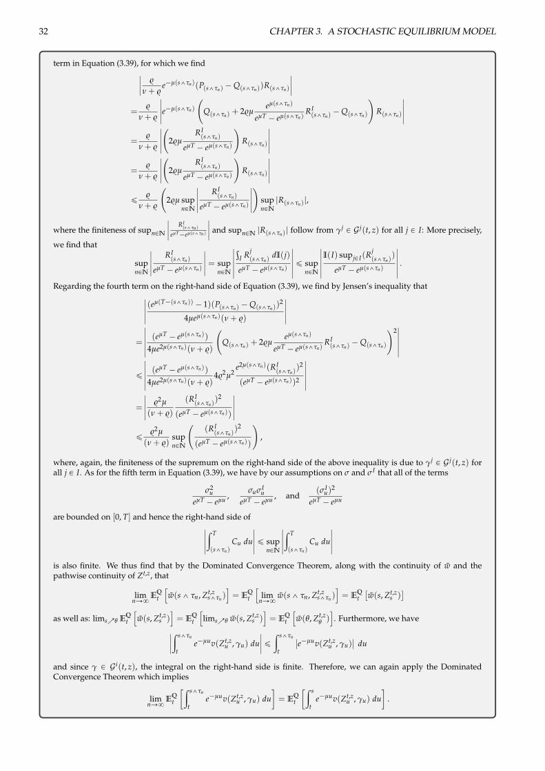
32 CHAPTER 3. A STOCHASTIC EQUILIBRIUM MODEL
term in Equation (3.39), for which we findˇˇ $
n + $
e´µ(s^tn)(P(s^tn) ´ Q(s^tn))R(s^tn)
ˇˇ
=$
n + $
ˇˇˇe
´µ(s^tn)
Q(s^tn) + 2$µ
eµ(s^tn)
eµT ´ eµ(s^tn)RI(s^tn)
´ Q(s^tn)
!R(s^tn)
ˇˇˇ
=$
n + $
ˇˇˇ
2$µ
RI(s^tn)
eµT ´ eµ(s^tn)
!R(s^tn)
ˇˇˇ
=$
n + $
ˇˇˇ
2$µ
RI(s^tn)
eµT ´ eµ(s^tn)
!R(s^tn)
ˇˇˇ
§ $
n + $
2$µ sup
nPN
ˇˇˇ
RI(s^tn)
eµT ´ eµ(s^tn)
ˇˇˇ
!supnPN
|R(s^tn)|,
where the finiteness of supnPN
ˇˇ RI
(s^tn )
eµT´eµ(s^tn )
ˇˇ and supnPN |R(s^tn)| follow from g
j P G j(t, z) for all j P I: More precisely,
we find that
supnPN
ˇˇˇ
RI(s^tn)
eµT ´ eµ(s^tn)
ˇˇˇ = sup
nPN
ˇˇˇ
≥I Rj
(s^tn)dI(j)
eµT ´ eµ(s^tn)
ˇˇˇ § sup
nPN
ˇˇˇI(I) supjPI(Rj
(s^tn))
eµT ´ eµ(s^tn)
ˇˇˇ .
Regarding the fourth term on the right-hand side of Equation (3.39), we find by Jensen’s inequality thatˇˇˇ(eµ(T´(s^tn)) ´ 1)(P(s^tn) ´ Q(s^tn))
2
4µeµ(s^tn)(n + $)
ˇˇˇ
=
ˇˇˇ(eµT ´ eµ(s^tn))
4µe2µ(s^tn)(n + $)
Q(s^tn) + 2$µ
eµ(s^tn)
eµT ´ eµ(s^tn)RI(s^tn)
´ Q(s^tn)
!2ˇˇˇ
§ˇˇˇ(eµT ´ eµ(s^tn))
4µe2µ(s^tn)(n + $)4$
2µ
2e2µ(s^tn)(RI
(s^tn))2
(eµT ´ eµ(s^tn))2
ˇˇˇ
=
ˇˇˇ
$
2µ
(n + $)
(RI(s^tn)
)2
(eµT ´ eµ(s^tn))
ˇˇˇ
§ $
2µ
(n + $)supnPN
(RI
(s^tn))2
(eµT ´ eµ(s^tn))
!,
where, again, the finiteness of the supremum on the right-hand side of the above inequality is due to g
j P G j(t, z) forall j P I. As for the fifth term in Equation (3.39), we have by our assumptions on s and s
I that all of the terms
s
2u
eµT ´ eµu ,sus
Iu
eµT ´ eµu , and(sI
u)2
eµT ´ eµu
are bounded on [0, T] and hence the right-hand side ofˇˇˇ
ª T
(s^tn)Cu du
ˇˇˇ § sup
nPN
ˇˇˇ
ª T
(s^tn)Cu du
ˇˇˇ
is also finite. We thus find that by the Dominated Convergence Theorem, along with the continuity of w and thepathwise continuity of Zt,z, that
limnÑ8
EQt
hw(s ^ tn, Zt,z
s^tn )i= EQ
t
hlim
nÑ8
w(s ^ tn, Zt,zs^tn )
i= EQ
t⇥w(s, Zt,z
s )⇤
as well as: limsÕq
EQt
hw(s, Zt,z
s )i= EQ
t
hlimsÕq
w(s, Zt,zs )i= EQ
t
hw(q, Zt,z
q
)i. Furthermore, we have
ˇˇª s^tn
te´µuv(Zt,z
u , gu) duˇˇ §
ª s^tn
t
ˇe´µuv(Zt,z
u , gu)ˇ
du
and since g P G i(t, z), the integral on the right-hand side is finite. Therefore, we can again apply the DominatedConvergence Theorem which implies
limnÑ8
EQt
ª s^tn
te´µuv(Zt,z
u , gu) du�= EQ
t
ª s
te´µuv(Zt,z
u , gu) du�
.
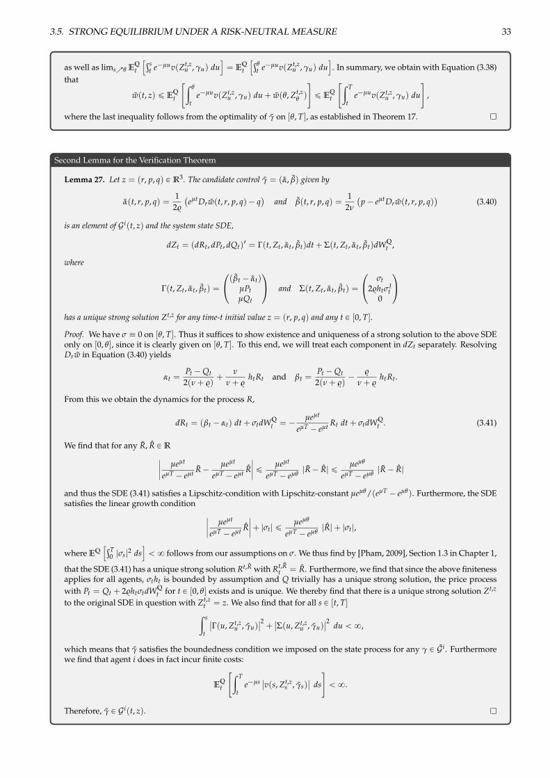
3.5. STRONG EQUILIBRIUM UNDER A RISK-NEUTRAL MEASURE 33
as well as limsÕq
EQt
h≥st e´µuv(Zt,z
u , gu) dui= EQ
t
h≥q
t e´µuv(Zt,zu , gu) du
i. In summary, we obtain with Equation (3.38)
that
w(t, z) § EQt
"ªq
te´µuv(Zt,z
u , gu) du + w(q, Zt,zq
)
#§ EQ
t
"ª T
te´µuv(Zt,z
u , gu) du
#,
where the last inequality follows from the optimality of g on [q, T], as established in Theorem 17.
Second Lemma for the Verification Theorem
Lemma 27. Let z = (r, p, q) P R3. The candidate control g = (a, b) given by
a(t, r, p, q) =1
2$
�eµtDrw(t, r, p, q) ´ q
�and b(t, r, p, q) =
12n
�p ´ eµtDrw(t, r, p, q)
�(3.40)
is an element of G i(t, z) and the system state SDE,
dZt = (dRt, dPt, dQt)1 = G(t, Zt, at, bt)dt + S(t, Zt, at, bt)dWQ
t ,
where
G(t, Zt, at, bt) =
0
@(bt ´ at)
µPtµQt
1
A and S(t, Zt, at, bt) =
0
@st
2$htsIt
0
1
A
has a unique strong solution Zt,z for any time-t initial value z = (r, p, q) and any t P [0, T].
Proof. We have s ” 0 on [q, T]. Thus it suffices to show existence and uniqueness of a strong solution to the above SDEonly on [0, q], since it is clearly given on [q, T]. To this end, we will treat each component in dZt separately. ResolvingDrw in Equation (3.40) yields
at =Pt ´ Qt2(n + $)
+n
n + $
htRt and bt =Pt ´ Qt2(n + $)
´ $
n + $
htRt.
From this we obtain the dynamics for the process R,
dRt = (bt ´ at) dt + stdWQt = ´ µeµt
eµT ´ eµt Rt dt + stdWQt . (3.41)
We find that for any R, R P R
ˇˇ µeµt
eµT ´ eµt R ´ µeµt
eµT ´ eµt Rˇˇ § µeµt
eµT ´ eµq
|R ´ R| § µeµq
eµT ´ eµq
|R ´ R|
and thus the SDE (3.41) satisfies a Lipschitz-condition with Lipschitz-constant µeµq/(eµT ´ eµq). Furthermore, the SDEsatisfies the linear growth condition
ˇˇ µeµt
eµT ´ eµt Rˇˇ + |st| § µeµq
eµT ´ eµq
|R| + |st|,
where EQh≥T
0 |ss|2 dsi
† 8 follows from our assumptions on s. We thus find by [Pham, 2009], Section 1.3 in Chapter 1,
that the SDE (3.41) has a unique strong solution Rt,R with Rt,Rt = R. Furthermore, we find that since the above finiteness
applies for all agents, stht is bounded by assumption and Q trivially has a unique strong solution, the price processwith Pt = Qt + 2$htstdWQ
t for t P [0, q] exists and is unique. We thereby find that there is a unique strong solution Zt,z
to the original SDE in question with Zt,zt = z. We also find that for all s P [t, T]
ª s
t
ˇG(u, Zt,z
u , gu)ˇ2+
ˇS(u, Zt,z
u , gu)ˇ2 du † 8,
which means that g satisfies the boundedness condition we imposed on the state process for any g P G i. Furthermorewe find that agent i does in fact incur finite costs:
EQt
"ª T
te´µs ˇ
v(s, Zt,zs , gs)
ˇds
#† 8.
Therefore, g P G i(t, z).
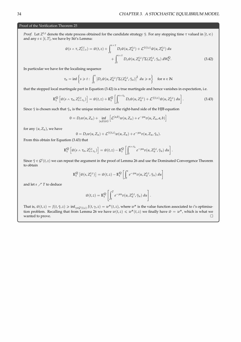
34 CHAPTER 3. A STOCHASTIC EQUILIBRIUM MODEL
Proof of the Verification Theorem 25
Proof. Let Zt,z denote the state process obtained for the candidate strategy g. For any stopping time t valued in [t, 8)and any s P [t, T], we have by Ito’s Lemma:
w(s ^ t, Zt,zs^t
) = w(t, z) +ª s^t
tDtw(u, Zt,z
u ) + Lg(t,z)w(u, Zt,zu ) du
+ª s^t
tDzw(u, Zt,z
u )1S(Zt,zu , gu) dWQ
u . (3.42)
In particular we have for the localising sequence
tn = inf"
s • t :ª s
t
ˇDzw(u, Zt,z
u )1S(Zt,zu , gu)
ˇ2 du • n*
for n P N
that the stopped local martingale part in Equation (3.42) is a true martingale and hence vanishes in expectation, i.e.
EQt
hw(s ^ tn, Zt,z
s^tn )i= w(t, z) + EQ
t
ª s^tn
tDtw(u, Zt,z
u ) + Lg(t,z)w(u, Zt,zu ) du
�. (3.43)
Since g is chosen such that gu is the unique minimiser on the right-hand side of the HJB equation
0 = Dtw(u, Zu) + inf(a,b)PG
hL(a,b)w(u, Zu) + e´µuv(u, Zu, a, b)
i
for any (u, Zu), we have0 = Dtw(u, Zu) + Lg(t,z)w(u, Zu) + e´µuv(u, Zu, gu).
From this obtain for Equation (3.43) that
EQt
hw(s ^ tn, Zt,z
s^tn )i= w(t, z) ´ EQ
t
ª s^tn
te´µuv(u, Zt,z
u , gu) du�
.
Since g P G i(t, z) we can repeat the argument in the proof of Lemma 26 and use the Dominated Convergence Theoremto obtain
EQt⇥w(s, Zt,z
s )⇤= w(t, z) ´ EQ
t
ª s
te´µuv(u, Zt,z
u , gu) du�
and let s Õ T to deduce
w(t, z) = EQt
"ª T
te´µuv(u, Zt,z
u , gu) du
#.
That is, w(t, z) = J(t, g, z) • infgPG i(t,z) J(t, g, z) = w˚(t, z), where w˚ is the value function associated to i’s optimisa-
tion problem. Recalling that from Lemma 26 we have w(t, z) § w˚(t, z) we finally have w = w˚, which is what wewanted to prove.
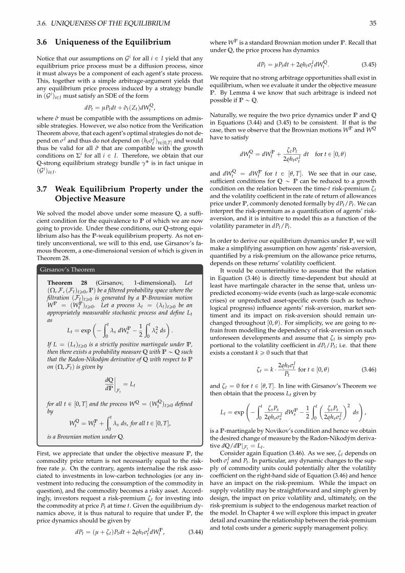
3.6. UNIQUENESS OF THE EQUILIBRIUM 35
3.6 Uniqueness of the Equilibrium
Notice that our assumptions on G i for all i P I yield that anyequilibrium price process must be a diffusion process, sinceit must always be a component of each agent’s state process.This, together with a simple arbitrage-argument yields thatany equilibrium price process induced by a strategy bundlein (G i)iPI must satisfy an SDE of the form
dPt = µPtdt + st(Zt)dWQt ,
where s must be compatible with the assumptions on admis-sible strategies. However, we also notice from the VerificationTheorem above, that each agent’s optimal strategies do not de-pend on s
I and thus do not depend on (htsIt )tP[0,T] and would
thus be valid for all s that are compatible with the growthconditions on Si for all i P I. Therefore, we obtain that ourQ-strong equilibrium strategy bundle g
˚ is in fact unique in(G i)iPI .
3.7 Weak Equilibrium Property under theObjective Measure
We solved the model above under some measure Q, a suffi-cient condition for the equivalence to P of which we are nowgoing to provide. Under these conditions, our Q-strong equi-librium also has the P-weak equilibrium property. As not en-tirely unconventional, we will to this end, use Girsanov’s fa-mous theorem, a one-dimensional version of which is given inTheorem 28.
Girsanov’s Theorem
Theorem 28 (Girsanov, 1-dimensional). Let(W,F , (Ft)t•0, P) be a filtered probability space where thefiltration (Ft)t•0 is generated by a P-Brownian motionWP = (WP
t )t•0. Let a process lt = (lt)t•0 be anappropriately measurable stochastic process and define Ltas
Lt = exp✓
´ª t
0ls dWP
s ´ 12
ª t
0l
2s ds
◆.
If L = (Lt)t•0 is a strictly positive martingale under P,then there exists a probability measure Q with P „ Q suchthat the Radon-Nikodym derivative of Q with respect to P
on (W,Ft) is given by
dQ
dP
ˇˇFt
= Lt
for all t P [0, T] and the process WQ = (WQt )t•0 defined
by
WQt = WP
t +ª t
0ls ds, for all t P [0, T],
is a Brownian motion under Q.
First, we appreciate that under the objective measure P, thecommodity price return is not necessarily equal to the risk-free rate µ. On the contrary, agents internalise the risk asso-ciated to investments in low-carbon technologies (or any in-vestment into reducing the consumption of the commodity inquestion), and the commodity becomes a risky asset. Accord-ingly, investors request a risk-premium zt for investing intothe commodity at price Pt at time t. Given the equilibrium dy-namics above, it is thus natural to require that under P, theprice dynamics should be given by
dPt = (µ + zt)Ptdt + 2$htsIt dWP
t , (3.44)
where WP is a standard Brownian motion under P. Recall thatunder Q, the price process has dynamics
dPt = µPtdt + 2$htsIt dWQ
t . (3.45)
We require that no strong arbitrage opportunities shall exist inequilibrium, when we evaluate it under the objective measureP. By Lemma 4 we know that such arbitrage is indeed notpossible if P „ Q.
Naturally, we require the two price dynamics under P and Q
in Equations (3.44) and (3.45) to be consistent. If that is thecase, then we observe that the Brownian motions WP and WQ
have to satisfy
dWQt = dWP
t +ztPt
2$htsIt
dt for t P [0, q)
and dWQt = dWP
t for t P [q, T]. We see that in our case,sufficient conditions for Q „ P can be reduced to a growthcondition on the relation between the time-t risk-premium ztand the volatility coefficient in the rate of return of allowancesprice under P, commonly denoted formally by dPt/Pt. We caninterpret the risk-premium as a quantification of agents’ risk-aversion, and it is intuitive to model this as a function of thevolatility parameter in dPt/Pt.
In order to derive our equilibrium dynamics under P, we willmake a simplifying assumption on how agents’ risk-aversion,quantified by a risk-premium on the allowance price returns,depends on these returns’ volatility coefficient.
It would be counterintuitive to assume that the relationin Equation (3.46) is directly time-dependent but should atleast have martingale character in the sense that, unless un-predicted economy-wide events (such as large-scale economiccrises) or unpredicted asset-specific events (such as techno-logical progress) influence agents’ risk-aversion, market sen-timent and its impact on risk-aversion should remain un-changed throughout [0, q). For simplicity, we are going to re-frain from modelling the dependency of risk-aversion on suchunforeseen developments and assume that zt is simply pro-portional to the volatility coefficient in dPt/Pt; i.e. that thereexists a constant k • 0 such that that
zt = k ¨ 2$htsIt
Ptfor t P [0, q) (3.46)
and zt = 0 for t P [q, T]. In line with Girsanov’s Theorem wethen obtain that the process Lt given by
Lt = exp
´
ª t
0
zsPs
2$hss
Is
dWPs ´ 1
2
ª t
0
✓zsPs
2$hss
Is
◆2ds
!,
is a P-martingale by Novikov’s condition and hence we obtainthe desired change of measure by the Radon-Nikodym deriva-tive dQ/dP|Ft = Lt.
Consider again Equation (3.46). As we see, zt depends onboth s
It and Pt. In particular, any dynamic changes to the sup-
ply of commodity units could potentially alter the volatilitycoefficient on the right-hand side of Equation (3.46) and hencehave an impact on the risk-premium. While the impact onsupply volatility may be straightforward and simply given bydesign, the impact on price volatility and, ultimately, on therisk-premium is subject to the endogenous market reaction ofthe model. In Chapter 4 we will explore this impact in greaterdetail and examine the relationship between the risk-premiumand total costs under a generic supply management policy.

36 CHAPTER 3. A STOCHASTIC EQUILIBRIUM MODEL
Chapter 4
Policy Relevance andApplication
In the following, we will focus our attention mainly on the en-tirety of regulated agents. In order to improve legibility, wethus omit the superscript I for aggregate quantities.
This chapter is devoted to extending our findings from Chap-ter 3 to a problem of optimal regulatory control that is partic-ularly relevant in the context of climate relevant resources. In-spired by the recent reform of the EU ETS to include a MarketStability Reserve (MSR) and the preceding political and aca-demic debate, we will consider a generic mechanism that ad-justs the supply of a resource in response to changes in agents’respective bank. We let f = ( ft)tP[0,T] denote the regulator’sex-ante allocation schedule. At each point in time t, the re-source allocation will be adjusted based on the bank Bt, whichitself is subject to exogenous shocks via the equilibrium dy-namics. Our mechanism will provide an abstraction of therules implemented by the EC MSR1.
The effects of any such and similar mechanism will depend onhow responsive it is in its operation. That is to say, how strongare the changes made to the regulatory environment whenchanges to exogenous factors occur? We want to concretisethe notion of responsiveness in order to gain an understand-ing of how a system can benefit in terms of cost-efficiency froma regulatory framework that can react to exogenous changes.In particular, we note that the effects of any mechanism simi-lar to the MSR depends on the degree by which the regulatoris willing to deviate from its ex-ante schedule f and, possi-bly, the ex-ante cap. We will find that the readiness to acceptex-post changes to the (expected) cap is intimately linked tothe responsiveness of the system – a phenomenon that we willexpound in some detail in the following section.
4.1 Cap Stringency and Responsiveness
Recall that in Section 3.5 we obtained a market equilibriumstrategy bundle (gi,˚)iPI where g
i,˚ = (ai,˚, b
i,˚), with
a
i,˚t =
Pt ´ Qt2(n + $)
+n
n + $
htRit
and b
i,˚t =
Pt ´ Qt2(n + $)
´ $
n + $
htRit,
for all t P [0, T]. Also recall that agent i’s time-t expected resid-ual abatement requirement is given by
Rit = EQ
t [Ei(t, T) ´ Ai(t, T)] ´ Bi
t + c.
Furthermore, recall that the induced equilibrium price processis given by
Pt = Qt + R02$µeµt
eµT ´ 1+ 2$µeµt
ª t
0
dxs
eµT ´ eµs ,
wheredxs = dEQ
s [E(0, T) ´ A(0, T)] .
The process x reflects changes in the agents’ expectationsabout their required abatement as a result of changes in theexpected total BAU deployment EQ
t [E(0, T)] and expected to-tal allocations EQ
t [A(0, T)]. With a supply adjustment mech-anism in place, changes to BAU deployment may partially orfully be offset by changes to the remaining expected alloca-tion: In case of an economic crisis such as most recently ob-served in 2007/08, we may witness (and indeed witnesses inthe example) a mounting bank of unused commodity unitsdue to a massive decline in expected production. Accordingly,the commodity’s market price dropped significantly and re-mained on a low level, causing doubt in the efficacy of thepolicy instrument altogether. In light of the long time hori-zons and substantial uncertainties on behalf of market partici-pants, these claims should not necessarily be rejected offhand.A responsive mechanism may compensate part of such shocksby reducing or increasing the resource allocation, such thatshocks are not transferred one-to-one onto the residual abate-ment requirement Rt and, as a side-effect, the price responseto unanticipated events may be mitigated.
Below, we will consider such a responsive mechanism, wherethe stringency by which the regulator adheres to the ex-antecap
≥T0 ftdt may be loosened in favour of regulatory respon-
siveness toward unanticipated events.2 In order to structureour analysis and interpretation, we will first establish someuseful notions and terminology. Firstly, consider the generalconcept of cap stringency: This term shall henceforth carry theconcept of how far the regulator is willing to deviate from theex-ante cap. In the example of emissions trading systems, theregulator may, depending on the bank of unused allowances,remove allowances from the allocation or introduce more al-lowances than previously planned. The higher the stringency,however, the less the regulator is willing to do so – a highercap stringency implies a lower propensity to deviate from theex-ante cap.
1Therein, less allowances will be made available next year than prescribed by the ex-ante schedule f , if the current year’s bank exceeds acertain threshold. Conversely, if the current bank has dropped below another (different) threshold, more allowances will be released to themarket than scheduled ex-ante. In our responsive mechanism, we do not assume any threshold levels but continuously adjust the allocationschedule for any values of Bi
t, i P I. However, we provide some insights into threshold levels later in the text.2Note that in climate relevant applications, the cap should typically only be altered within an acceptable range; i.e. up to a GHG limit that
prevents catastrophic damages to the environment. In the following we neglect this constraint for tractability reasons but note that within thisrange, the optimal instrument is not necessarily a border solution on the policy spectrum.
37
38 CHAPTER 4. POLICY RELEVANCE AND APPLICATION
Note that we will use the term cap stringency only in a quali-tative sense. In the interest of useful quantification, we intro-duce another notion, complementary to cap stringency: Eachtime the resource allocation is adjusted, we assume that theregulator does so based on a fixed set of rules and on the bankof unused commodity units. The farther the bank deviatesfrom the reference point c P R, the stronger the response willbe in absolute terms. However, we will let the regulator de-cide ex-ante on the relative strength of his response; that is tosay: the regulator may decide ex-ante how strong the responseis in relation to the difference |Bt ´ c|. A relatively ‘weak’ re-sponse will let the bank deviate more freely from the pointc, which preserves the ex-ante cap to a large extend. In thiscase, the mechanism is only slightly responsive, while the capstringency is rather high. In Section 4.2, we will quantify thisrelative responsiveness in terms of a parameter d • 0, labelledadjustment rate. With a high adjustment rate, the strength ofthe response, relative to the difference |Bt ´ c| will be high,which may require the regulator to deviate farther from theex-ante cap. In that sense, the terms cap stringency and respon-siveness, the latter being quantified by the adjustment rate, rep-resent complementary notions, which will be quite useful inthe following.
4.2 A Regulatory Mechanism with Ad-justable Responsiveness
In this section, we construct a responsive mechanism that cov-ers a spectrum of policies between a pure price instrumentand a pure quantity instrument by means of parameterisa-tion with an adjustment rate d. This will lay the ground forSection 4.3, where we will show how the regulator can iden-tify an adjustment rate that minimises expected aggregate to-tal abatement costs. In particular, we will identify a trade-offbetween a high responsiveness, which, as we shall see, lowersthe agents’ costs of adjusting to shocks on the one hand; and alow responsiveness, which yields potential for agents to bene-fit from inter-temporal cost-saving opportunities on the otherhand.
We begin by indexing the regulator’s allocation adjustments tothe aggregate bank of commodity units: At each time t P [0, T],if the current aggregate bank is above the fixed level c P R, welet a fraction ddt (where d • 0) of the difference |Bi
t ´ c| beinstantaneously removed from the allocation, for each i P I.Conversely, if the aggregate bank drops below the level c, theallocation is increased by d ¨ |Bi
t ´ c|dt, compared to the ex-ante schedule.3 Here, we abstract the workings of the MSR, inwhich allowances are removed from (or added to) next year’sallocation and set aside into (or taken from) a so-called ‘re-serve’. For the purpose of an analysis of the policy spectrumin our continuous-time setting, however, we opt for an instan-taneous allocation adjustment.
We point out that for each agent i’s optimisation problem inthe previous chapter to be applicable, any assumptions on theBAU deployment process, together with the aggregate systemdynamics, must admit a representation of x
i as dx
it = s
it dWQ
t ,where the process s
i is deterministic and bounded with s
i ” 0on [q, T]. Regarding the random perturbations of BAU deploy-ment, we here make a fairly simple assumption for the sakeof tractability: Let each agent i’s cumulated BAU deployment
process be given by
Ei(0, t) =ª t
0gi
s ds +ª t
0k
is dWQ
s ,
where gi and k
i shall be some deterministic and bounded pro-cesses and k
it = 0 for t P [q, T]. As we shall see as a by-
product of the following Proposition 29, our responsive mech-anism and the above assumption on BAU deployment are infact compatible with the assumption that dx
it = s
it dWQ
t ands
i will indeed turn out to be deterministic and bounded withs
i ” 0 on [q, T].
We can express the instantaneous change in the aggregatebank of commodity units by
dBt = ftdt + d(c ´ Bt)dt ´ gtdt ´ ktdWQt + atdt.
Note that in contrast to the EC MSR, there is neither an explicitnor an implicit announcement that those units removed fromthe allocation will be re-introduced to the market later-on, or(in case of additional allocation) vice-versa. With our mecha-nism, each adjustment to the allocation schedule carries withit an instantaneous deviation from the ex-ante cap at the sameamount, although the expected ex-post cap may be altered by adifferent amount, subject to the market’s endogenous reactionand future allocation adjustments. For example, an instan-taneous allocation adjustment may remove some commodityunits from the allocation, but future allocation adjustmentsare expected to re-introduce some of those units later-on. Ac-cordingly, the time-t instantaneous change dEQ
t [A(0, T)] to ex-pected total allocations may differ from d ¨ |Bt ´ c| dt and issubject to the equilibrium dynamics. We will solve this inter-dependency in Proposition 29, where we derive the aggregatebank’s dynamics in equilibrium, under the adjustment mech-anism. This step in our analysis will prove fundamental tothe quantification of aggregate expected compliance costs andhence for the design of an optimal policy, which we will dis-cuss in Section 4.3.
For the purpose of demonstration, first consider the case of arather large adjustment rate d, close to 100% per time-unit. Inthis case, almost the entire difference |Bt ´ c| is removed fromor added to the allocation, which tightens the bank closelyaround the level c. In this case, the cap may have to be ad-justed heavily, depending on the level of shocks to BAU de-ployment that the regulator has to compensate. Accordingly,we say that this case requires an almost fully floating cap. Andsince the price is effectively fixed, we are close to the pure priceextreme of the policy spectrum.
Towards the other end of the policy spectrum lies the casewhere the adjustment rate d is close to zero. Here, the allo-cation adjustments only partially compensate shocks to BAUdeployment, and only to a small extend. The bank thus fluc-tuates relatively freely from the level c, and agent’s abatementresponds heavily to changes in BAU deployment. Accord-ingly, those shocks are almost fully reflected in the marketprice. The small volume of allocation adjustments requiresthe regulator to alter the ex-ante cap only slightly and thus thepolicy instrument is close to a pure quantity instrument, suchas a ‘pure’ emissions trading system (e.g. the EU ETS beforethe introduction of additional measures like the MSR). When
3When discretising the model, the time increment dt may be replaced by some fixed timespan (e.g. a year) such that the following exemplaryintuition holds: d would correspond to the percentage of |Bt ´ c| that is added to or removed from next year’s allocation. In our continuous-timesetting, d is simply the adjustment rate of the regulator’s allocation.
4.2. A REGULATORY MECHANISM WITH ADJUSTABLE RESPONSIVENESS 39
d = 0, there are no adjustments to the allocation and, accord-ingly, no adjustments to the cap, which simply results in apure quantity instrument.
For a given adjustment rate level d • 0, consider the aggregateabatement in equilibrium:
at = µeµt R0(d)
eµT ´ 1+ µeµt
ª t
0
dxs(d)
eµT ´ eµs (4.1)
Recall that the process x represents changes to the agents’ ex-pectations of BAU deployment versus allocations. With theresponsive mechanism in place, x is subject to the adjustmentrate d, and the abatement curve responds to the mechanism,the allocation adjustments of which, in turn, respond to the ag-gregate abatement curve. (We will solve this inter-dependencyin Proposition 29.) Consider the first term on the right-handside of Equation (4.1), where R0(d) is the expected total re-quired abatement, given only the information present at time0. If no unanticipated events were to occur (that is to say, ifx ” 0) the second term in Equation (4.1) would vanish andagents would simply spread their abatement effort over time,taking into account the cost differences imposed by the inter-est rate µ.
When unanticipated changes to future required abatementoccur, the respective information is continuously incorporatedinto agents’ abatement behaviour, as represented by the sec-ond term on the right-hand side of Equation (4.1). At eachtime s P [0, t], any changes dxs to expected required abatementare spread over time, taking into account the interest rate µ.
Recall that unanticipated changes to the required abatement,given by dxs = dEQ
s [E(0, T) ´ A(0, T)], incorporate bothchanges to the expected total BAU deployment EQ
s [E(0, T)], aswell as changes to the expected total allocations EQ
s [A(0, T)].Obviously, when changes in expected total BAU deploymentwere perfectly compensated by matching changes in total ex-pected allocations (i.e. in the hypothetical4 case d Ñ 8), therewould be no changes to the expected required abatement. This
case would correspond to a perfectly responsive mechanism:The term dxs would vanish and the abatement would simplyincrease at the rate µ, just like in the deterministic case. Andsince, in equilibrium, the market price equals marginal abate-ment costs, the price would remain constant in discountedterms. If such a perfect compensation of dEQ
s [E(0, T)] bydEQ
s [A(0, T)] would be present throughout the entire regu-lated period [0, T], the mechanism would be fully responsiveand would, in fact, realise a pure price instrument, since themarket would effectively fix the price without any deviationsfrom external shocks. In terms of responsiveness, the mecha-nism would thus lie on what we refer to as the price extreme of apolicy spectrum, along which different degrees of responsive-ness may be realised. On the other end of this spectrum lies apure quantity instrument, where d = 0 and the cap is never re-laxed or tightened; and where , accordingly, there is no adjust-ment to expected total allocations EQ
s [A(0, T)]. In this case, theprice is effectively allowed to float freely, as the adjustment toshocks is fully borne by the agents, through their adjustmentin abatement.
Notice that a responsive mechanism can compensate some ofthe shocks to BAU deployment and thus may reduce costs ofadjustment on behalf of the agents. However, it also limits thetemporal flexibility provided to agents and may therefore re-duce the cost-efficiency of a quantity instrument such as emis-sions trading systems. In the extreme case of a fully responsivemechanism, the market priced is effectively fixed, turning thesystem into a de-facto tax. In what follows, we will examinethis trade-off more closely and show how it can be solved tothe end of inferring a mechanism that is optimal in terms ofagents’ expected aggregate total abatement costs.
The Bank under the Responsive MechanismWe will now derive a closed-form expression for the time-t(aggregate) bank of unused commodity units.
The Bank under the Responsive Mechanism in Closed-Form
Proposition 29. The time-t bank under the responsive mechanism is given in closed-form by
Bt = B0e´dt +µ(eµt ´ e´dt)
(d + µ)(eµT ´ 1)R0 ´ eµt
Vt(d, r)
ª t
0e´µs Vs(d, r)ks dWQ
s +ª t
0ed(s´t)( fs ´ gs + dc) ds,
where
R0 = EQ0 [Y(0, T)] = ´ (d + µ)(eµT ´ 1)
µ(eµT ´ e´dT)
B0e´dT +
ª T
0ed(s´T)( fs ´ gs + dc) ds ´ c
!.
Proof. For convenience, we define the process # = (#t)tP[0,T] by d#t = ktdWQt . We then have the dynamics of the
aggregate bank given bydBt = ftdt + d(c ´ Bt)dt ´ gtdt ´ d#t + atdt, (4.2)
which is solved by the following expression for the time-t bank:
Bt = B0e´dt +ª t
0ed(s´t)(as + fs + dc ´ gs) ds ´
ª t
0ed(s´t) d#s (4.3)
Notice that the above equation expresses Bt in terms of the (past and present) abatement (as)sP[0,t], which itself depends
on the dynamics of the (expected) bank through EQs [Y(0, T)], 0 § s § t. More precisely we have that
at = µeµt R0eµT ´ 1
+ µeµtª t
0
dEQs [Y(0, T)]
eµT ´ eµs ,
4We forego a rigorous treatment of the limit case in mathematical terms, since our interest lies on the spectrum of policies rather than theextreme case of a pure tax.
40 CHAPTER 4. POLICY RELEVANCE AND APPLICATION
where, in turn, the dynamics of dEQs [Y(0, T)] are given by
dEQt [Y(0, T)] = dEQ
t
"ª T
0d#s ´
ª T
0dBs ds
#= d#t + ddEQ
t
"ª T
0Bs ds
#.
In order to obtain at and Bt in closed-form, we thus need to solve the above interdependencies between the processesa and B. In order to simplify notation, we first recall that
ht =µeµt
eµT ´ eµt .
Using this notation, the dynamics of aggregate abatement can be expressed as
dat = µatdt + htdEQt [Y(0, T)]. (4.4)
We also recall that by the terminal constraint, we have that dEQt [BT ] = 0 is satisfied for all t P [0, T], which we apply to
Equation (4.3). Isolating the term depending on a then yields
dEQt
"ª T
0eds
as ds
#= dEQ
t
"ª T
0eds(gs ´ fs ´ dc) ds ´ B0 +
ª T
0eds d#s
#= edtd#t. (4.5)
We can make use of the dynamics of a in equation (4.4) in order to establish:ª t
0aseds ds =
edt
d + µ
✓at ´ a0e´dt ´
ª t
0ed(s´t)hs dEQ
s [Y(0, T)]◆
.
The above equation, together with Equation (4.5), then yields:
dEQt [Y(0, T)] =
Vt(d, µ)ht
d#t, (4.6)
where Vt(d, µ) = (d + µ)/(e(d+µ)(T´t) ´ 1). From this we finally obtain
Bt = B0e´dt +µ(eµt ´ e´dt)
(d + µ)(eµT ´ 1)R0 ´ eµt
Vt(d, µ)
ª t
0e´µs Vs(d, µ) d#s +
ª t
0ed(s´t)( fs ´ gs + dc) ds. (4.7)
Note that R0 = EQ0 [Y(0, T)]. Using the compliance condition BT = c, we can now derive the expression for EQ
0 [Y(0, T)]:
EQ0 [Y(0, T)] = ´ (d + µ)(eµT ´ 1)
µ(eµT ´ e´dT)
B0e´dT +
ª T
0ed(s´T)( fs ´ gs + dc) ds ´ c
!.
Thus, the time-t bank Bt is indeed determined in closed-form by Equation (4.7).
Notice that by Equation (4.6), the proof of Proposition 29yields as a by-product that dxt = stdWQ
t , where s is deter-ministic and bounded with st = 0 for t P [q, T]. Therefore,under the responsive mechanism, the optimisation problemfor each agent in the previous chapter is indeed valid and theequilibrium thus persists under this regulation.
In Figure 4.1 we showcase the relation between the adjustmentrate and the aggregate bank under an exemplary parameteri-sation. The figure exemplifies how the aggregate bank is dis-persed, according to its quantiles at 90% confidence level, withand without a positive adjustment rate. In both cases, we no-tice that by spreading their abatement effort over time, agentsstart to accumulate a bank of commodity units at the begin-ning of the regulated timeframe, and draw this bank down astime moves forward and the terminal constraint approaches.However, agents’ banking behaviour is noticeably influencedby whether or not the adjustment mechanism is in place: In theleft-hand diagram, the adjustment rate is set to zero. In thiscase, agents adjust their yearly abatement in response to un-compensated shocks, bearing the full costs of adjusting theirstrategy each time. Accordingly, the full extend of exogenous
shocks is reflected in the realised banking curves, illustratedin the respective quantiles.
The right-hand diagram illustrates the case where the adjust-ment rate is set to 5% per time-unit. In this case, the mecha-nism adjusts the allocation up or down, based on the aggre-gate bank. The realised banking curves in each scenario arethus dispersed more tightly, illustrated by their quantiles. Interms of the confidence level, we can thus say that the bankis kept within a ‘tighter’ band. Furthermore, the agents bearlower costs of adjusting to exogenous shocks, since their effectis partially compensated through adjustments to the alloca-tion (and the cap). Notice, however, that agents’ banking be-haviour is also affected by anticipated allocation adjustments,which influences the banking behaviour - even in the absenceof shocks. The regulator thus interferes with agents’ inter-temporal optimisation, potentially reducing the value of theirinter-temporal flexibility. We will examine this phenomenonmore closely in the next section, where we calculate total ag-gregate abatement costs as a function of the adjustment rate,in order to pick the most cost-efficient policy solution.
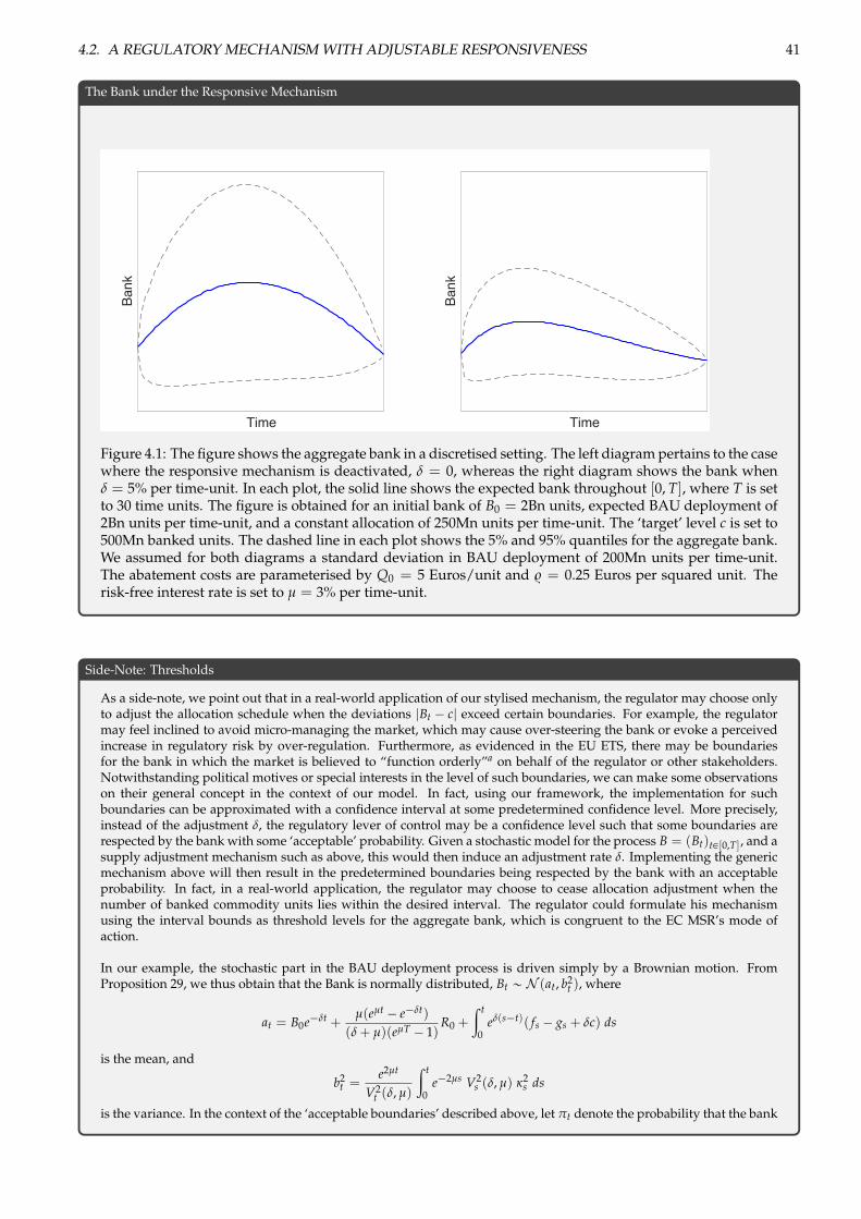
4.2. A REGULATORY MECHANISM WITH ADJUSTABLE RESPONSIVENESS 41
The Bank under the Responsive Mechanism
Time
Bank
Time
Bank
Figure 4.1: The figure shows the aggregate bank in a discretised setting. The left diagram pertains to the casewhere the responsive mechanism is deactivated, d = 0, whereas the right diagram shows the bank whend = 5% per time-unit. In each plot, the solid line shows the expected bank throughout [0, T], where T is setto 30 time units. The figure is obtained for an initial bank of B0 = 2Bn units, expected BAU deployment of2Bn units per time-unit, and a constant allocation of 250Mn units per time-unit. The ‘target’ level c is set to500Mn banked units. The dashed line in each plot shows the 5% and 95% quantiles for the aggregate bank.We assumed for both diagrams a standard deviation in BAU deployment of 200Mn units per time-unit.The abatement costs are parameterised by Q0 = 5 Euros/unit and $ = 0.25 Euros per squared unit. Therisk-free interest rate is set to µ = 3% per time-unit.
Side-Note: Thresholds
As a side-note, we point out that in a real-world application of our stylised mechanism, the regulator may choose onlyto adjust the allocation schedule when the deviations |Bt ´ c| exceed certain boundaries. For example, the regulatormay feel inclined to avoid micro-managing the market, which may cause over-steering the bank or evoke a perceivedincrease in regulatory risk by over-regulation. Furthermore, as evidenced in the EU ETS, there may be boundariesfor the bank in which the market is believed to “function orderly”a on behalf of the regulator or other stakeholders.Notwithstanding political motives or special interests in the level of such boundaries, we can make some observationson their general concept in the context of our model. In fact, using our framework, the implementation for suchboundaries can be approximated with a confidence interval at some predetermined confidence level. More precisely,instead of the adjustment d, the regulatory lever of control may be a confidence level such that some boundaries arerespected by the bank with some ‘acceptable’ probability. Given a stochastic model for the process B = (Bt)tP[0,T], and asupply adjustment mechanism such as above, this would then induce an adjustment rate d. Implementing the genericmechanism above will then result in the predetermined boundaries being respected by the bank with an acceptableprobability. In fact, in a real-world application, the regulator may choose to cease allocation adjustment when thenumber of banked commodity units lies within the desired interval. The regulator could formulate his mechanismusing the interval bounds as threshold levels for the aggregate bank, which is congruent to the EC MSR’s mode ofaction.
In our example, the stochastic part in the BAU deployment process is driven simply by a Brownian motion. FromProposition 29, we thus obtain that the Bank is normally distributed, Bt „ N (at, b2
t ), where
at = B0e´dt +µ(eµt ´ e´dt)
(d + µ)(eµT ´ 1)R0 +
ª t
0ed(s´t)( fs ´ gs + dc) ds
is the mean, and
b2t =
e2µt
V2t (d, µ)
ª t
0e´2µs V2
s (d, µ) k
2s ds
is the variance. In the context of the ‘acceptable boundaries’ described above, let pt denote the probability that the bank
42 CHAPTER 4. POLICY RELEVANCE AND APPLICATION
stays within the band [lt, ut]. We then have
pt = F⇣
d(1)t
⌘´ F
⇣d(2)t
⌘,
where F(¨) represents the cumulative distribution function of the standard normal distribution and the parameters d(1)t
and d(2)t are given by
d(1)t =ut ´ at
btand d(2)t =
lt ´ atbt
.
As anticipated, the probability pt can now be expressed as a function Ct(d) = pt. The respective bank interval can nowbe maintained with a confidence level pt if the adjustment rate d is set to C´1
t (pt) and vice-versa.
aSee [The European Commission, 2012].
4.3 Expected Total Abatement Costs andPolicy Implications
The objective of this section is to show how the regulator canselect an adjustment rate that minimises total aggregate abate-ment costs in expectation. Note that in the sense of regula-tory optimisation, our analysis ignores the societal benefit ofreducing the total aggregate deployment under the new regu-lation. That is, the benefit of implementing a specific expectedex-post cap is explicitly omitted in the optimisation problemand total economic costs are isolated. Our reason for doing sois based on our main application: Recall that CO2, as well ascomparable greenhouse gases are stock pollutants. As pointedout by [Newell and Pizer, 2008], the marginal benefit curve (ofreducing emissions) is flat compared to the marginal (aggre-gate) abatement cost curve (as long as total emissions do notexceed the boundary of catastrophic implications): The bene-fit of reducing e.g. 1 billion tonnes of GHG more than neces-sary for the avoidance of catastrophic damages is negligible,compared to the costs of implementing that additional restric-
tion.5 Hence, maximising societal benefits minus economiccosts can be well approximated by minimising only economiccosts (given the above boundary). In the interest of tractabil-ity, we ignore the ‘catastrophic’ boundary condition, but pointout that in a real-world application, some total cap should notbe exceeded by allocation adjustments. The EC MSR, for ex-ample, implements this condition by ceasing additional allo-cations, once a previously filled reserve runs empty.
In order to illustrate how different adjustment rates affect ex-pected total aggregate abatement costs, we first express thosecosts explicitly in Corollary 30. Note that we ignore total trad-ing costs for simplicity since this would not add any qualita-tive value to our discussion later-on. Furthermore, we calcu-late the expectation of costs under the risk-neutral measureQ, in order to first illustrate the effects of our mechanismirrespective of the level or functional representation of risk-aversion. In Section 4.3.2, we will then examine the effects ofrisk-aversion more closely by considering realised costs andrisk-premia under different levels for d.
Expected Total Aggregate Abatement Costs
Corollary 30. Expected total aggregate abatement costs are given by
EQ
"ª T
0e´µt
⇣Qtat + $a
2t
⌘dt
#= Q0R0 + $µ
R20
eµT ´ 1+ $µ
ª T
0
dxEQ [Y(0, T)]yt�eµT ´ eµt� ,
where x¨y refers to quadratic variation.
Proof. We first notice that we have
EQ
"ª T
0e´µt
⇣Qtat + $a
2t
⌘dt
#= EQ
"ª T
0e´µtQt at dt
#+ $ EQ
"ª T
0e´µt
a
2t dt
#
= Q0 EQ
"ª T
0at dt
#+ $ EQ
"ª T
0e´µt
a
2t dt
#. (4.8)
Also, recall that we have for all d
ª t
0eds
asds =1
d + µ
✓edt
at ´ a0 ´ª t
0edshsdEQ
s [Y(0, T)]◆
.
We can use the above equation with d = 0 and t = T to resolve the first term on the right-hand side of Equation (4.8):
Q0 EQ
"ª T
0at dt
#=
Q0µ
EQ [aT ] ´ a0 ´ EQ
"ª T
0htdEQ
t [Y(0, T)]
#!
=Q0µ
⇣EQ [aT ] ´ a0
⌘.
5Note, however, that an adjustment rate that benefits agents by making the system more responsive may, lead to a lower ex-post cap. Incontrast to societal benefits, the economic benefits in terms of cost reduction through responsiveness are included in our cost analysis.
4.3. EXPECTED TOTAL ABATEMENT COSTS AND POLICY IMPLICATIONS 43
By the expression for aggregate abatement we obtain
EQ [aT ] ´ a0 = µeµT R0eµT ´ 1
´ µ
R0eµT ´ 1
= µR0.
We thus arrive at
Q0 EQ
"ª T
0at dt
#= Q0R0. (4.9)
Regarding the second term on the right-hand side of Equation (4.8), we have
ª T
0e´µt
a
2t dt = ´ 1
µ
ª T
0a
2t de´µt =
1µ
a
20 ´ e´µT
a
2T +
ª T
0e´µtda
2t
!.
We can use the fact that
da
2t = 2atdat + dxayt = 2at(µatdt + htdEQ
t [Y(0, T)]) + h2t dxEQ [Y(0, T)]yt
= 2µa
2t dt + 2athtdEQ
t [Y(0, T)] + h2t dxEQ [Y(0, T)]yt
to deduce thatª T
0e´µt
a
2t dt
=1µ
a
20 ´ e´µT
a
2T +
ª T
0e´µt2µa
2t dt +
ª T
0e´µt2athtdEQ
t [Y(0, T)] +ª T
0e´µth2
t dxEQ [Y(0, T)]yt
!
=1µ
a
20 ´ e´µT
a
2T +
ª T
0e´µt2athtdEQ
t [Y(0, T)] +ª T
0e´µth2
t dxEQ [Y(0, T)]yt
!+ 2
ª T
0e´µt
a
2t dt.
This implies that
ª T
0e´µt
a
2t dt =
1µ
e´µT
a
2T ´ a
20 ´
ª T
0e´µt2athtdEQ
t [Y(0, T)] ´ª T
0e´µth2
t dxEQ [Y(0, T)]yt
!
and consequently
$ EQ
"ª T
0e´µt
a
2t dt
#=
$
µ
e´µT
✓VarQ [aT ] +
⇣EQ [aT ]
⌘2◆
´ a
20 ´
ª T
0e´µth2
t dxEQ [Y(0, T)]yt
!,
where we used, in particular, that dxEQ [Y(0, T)]yt/dt is deterministic. Since dEQt [Y(0, T)]/dWt is deterministic and
bounded in [0, T] we obtain
e´µTVarQ [aT ] = e´µTµ
2e2µTª T
0
dxEQ [Y(0, T)]yt�eµT ´ eµt�2 = µ
2ª T
0
eµTdxEQ [Y(0, T)]yt�eµT ´ eµt�2 .
Also notice that ª T
0e´µth2
t dxEQ [Y(0, T)]yt = µ
2ª T
0
eµtdxEQ [Y(0, T)]yt�eµT ´ eµt�2
and hence
e´µTVarQ [aT ] ´ª T
0e´µth2
t dxEQ [Y(0, T)]yt = µ
2ª T
0
dxEQ [Y(0, T)]yt�eµT ´ eµt� .
Furthermore,
e´µT⇣
EQ [aT ]⌘2 ´ a
20 = e´µT
µ
2e2µT R20
(eµT ´ 1)2 ´ µ
2 R20
(eµT ´ 1)2 = µ
2 R20
eµT ´ 1.
Together, we find that
$ EQ
"ª T
0e´µt
a
2t dt
#= $µ
R20
eµT ´ 1+ $µ
ª T
0
dxEQ [Y(0, T)]yt�eµT ´ eµt� . (4.10)
Equations (4.9) and (4.10) together yield
EQ
"ª T
0e´µt
⇣Qtat + $a
2t
⌘dt
#= Q0R0 + $µ
R20
eµT ´ 1+ $µ
ª T
0
dxEQ [Y(0, T)]yt�eµT ´ eµt� ,
which is what we wanted to prove.
44 CHAPTER 4. POLICY RELEVANCE AND APPLICATION
4.3.1 The Optimal Adjustment RateWe will now use our closed-form expression for expected totalaggregate abatement costs to discuss the trade-off the regula-tor faces when selecting a cost-minimising adjustment rate d.
On the one hand, recall that due to exogenous shocks to BAUdeployment, the agents continuously adapt their strategies,which increases their total costs. The total of necessary ad-justments can be reduced by the implementation of a positiveadjustment rate. And, with a very large adjustment rate, closeto 100% per time-unit, the regulator can almost fully eradi-cate any variation in agents’ expected abatement requirement,leading to a de-facto fixed price policy. It is therefore intuitivethat the higher the adjustment rate, the lower the cost of adjust-ments on behalf of agents should be.
On the other hand, agents use their ability to bank commodityunits throughout the regulated timeframe to minimise theirexpected total costs. The profitability or viability of inter-temporal cost-saving opportunities may be affected by a pos-itive adjustment rate: The higher the adjustment rate, the‘tighter’ the bank is forced to fluctuate around the level c, andinter-temporal cost-saving opportunities are more and morereduced as d increases.
Consider the total costs derived in Corollary 30; i.e.
Q0R0 + $µ
R20
eµT ´ 1+ $µ
ª T
0
dxxyt�eµT ´ eµt� , (4.11)
where xt = EQt [Y(0, T)].
Analytically, we can identify the above-mentioned trade-off inthe interaction of the three summands on the right-hand sideof Equation (4.11): The first two terms Q0R0 and $µR2
0/(eµT ´1) quantify the costs in the absence of uncertainty. Hereinwe can, in particular, isolate any effects the adjustment ratehas on total costs that are irrespective of responsiveness andits benefits. To that end, consider the initial expected abate-ment requirement R0 = E0 [E(0, T) ´ A(0, T)] ´ B0 + c. First,consider the case where the initial bank B0 is higher than c(e.g. B0 ° 0 and c = 0). In this case, if d ° 0, the mech-anism will, in expectation, decrease the total cap, comparedto the case where d = 0 – and this effect will intensify withan increasing adjustment rate. Accordingly, the first term inEquation (4.11), Q0R0, will increase due to an increasing ini-tial abatement requirement R0. Conversely, if B0 † c, the capwill increase with an increasing d ° 0, and the term Q0R0 willdecrease accordingly.
As for the second term on the right-hand side of Equation(4.11), i.e. $µR2
0/(eµT ´ 1), recall that the higher the adjust-
ment rate, the tighter the bank is kept around c. Accord-ingly, inter-temporal optimisation opportunities will be af-fected since strategies that entail a large bank are no longeras profitable or viable. Since $ parameterises the costs as-sociated to variations in abatement, agents have an incen-tive to spread their abatement across the regulated timeframe.This leads to the typical banking behaviour illustrated in Fig-ure 4.1: Agents first accumulate commodity units and thensteadily draw them down (cf. [Rubin, 1996] and [Schennach,2000]). The associated cost-saving opportunities, however,are affected by a positive adjustment rate, since the benefitsof such banking behaviour is partially offset by the mecha-nisms propensity to diminish a larger bank. Accordingly, thebanking curve is skewed, compared to the case where d = 0,increasing costs quadratically whenever R0 is increased byd ° 0.
As for the third term on the right-hand side of Equation(4.11), recall that dxxyt is the time-t quadratic variation ofthe expected total abatement requirement. Accordingly,$µ
≥T0
dxxyt(eµT
´eµt)captures costs due to agents’ strategy adjust-
ments. The regulator can reduce those costs by increasingthe adjustment rate d: The more responsive the system is, thesmaller the total adjustments become on behalf of the agents.The variability in expected required abatement is reduced byan increasing d, decreasing the above term in Equation (4.11).
As we can see, there is an inherent trade-off regarding ex-pected aggregate total abatement costs when selecting an ad-justment rate. We illustrate this trade-off in Figure 4.2, whichshows expected aggregate total abatement costs as a functionof the adjustment rate, computed for a set of illustrative pa-rameters.
Consider the results shown in Figure 4.2. For an adjustmentrate of zero (on the left end of the horizontal axis), whenthe cap is unaffected, the policy instrument lies at the fixed-cap end of the spectrum, as implemented in the former EUETS setup, before recent reforms took place. At this extreme,agents spread their abatement effort over time, taking into ac-count the risk-free rate µ. The presence of exogenous shocks,however, inflict costs through the adjustments that agentsmake in their response. When the adjustment rate is gradu-ally increased, these adjustments decrease, which in turn re-duces costs through strategy adjustments. Towards the fixed-price end of the spectrum (towards the right end of the hori-zontal axis), however, costs start to increase again: The costsof foregone cost savings from inter-temporal cost-saving op-portunities surpass the benefits from the mechanism’s respon-siveness. The loss of benefits from exploiting differences inmarginal abatement costs across time exceed the agents’ costsavings caused from shock-mitigation by the mechanism.
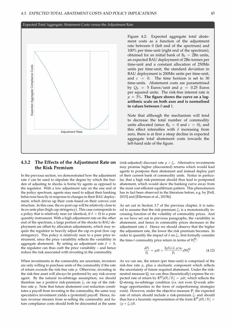
4.3. EXPECTED TOTAL ABATEMENT COSTS AND POLICY IMPLICATIONS 45
Expected Total Aggregate Abatement Costs versus the Adjustment Rate
Adjustment Rate
Expe
cted
Agg
rega
te C
ompl
ianc
e C
osts
Figure 4.2: Expected aggregate total abate-ment costs as a function of the adjustmentrate between 0 (left end of the spectrum) and100% per time-unit (right end of the spectrum),obtained for an initial bank of B0 = 2Bn units,an expected BAU deployment of 2Bn tonnes pertime-unit and a constant allocation of 250Mnunits per time-unit; the standard deviation inBAU deployment is 200Mn units per time-unit,and c = 0. The time horizon is set to 30time-units. Abatement costs are parametrisedby Q0 = 5 Euros/unit and $ = 0.25 Eurosper squared units. The risk-free interest rate isµ = 3%. The figure shows the curve on a log-arithmic scale on both axes and is normalisedto values between 0 and 1.
Note that although the mechanism will tendto decrease the total number of commodityunits allocated (since B0 ° 0 and c = 0), andthis effect intensifies with d increasing fromzero, there is at first a steep decline in expectedaggregate total abatement costs towards theleft-hand side of the figure.
4.3.2 The Effects of the Adjustment Rate onthe Risk Premium
In the previous section, we demonstrated how the adjustmentrate d can be used to stipulate the degree by which the bur-den of adjusting to shocks is borne by agents as opposed tothe regulator. With a low adjustment rate on the one end ofthe policy spectrum, agents may need to adjust their bankingbehaviour heavily in response to changes in their BAU deploy-ment, which drives up their costs based on their convex coststructure. In this case, the ex-post cap will be relatively close toits ex-ante plan (high cap stringency). This case corresponds toa policy that is relatively near (or identical, if d = 0) to a purequantity instrument. With a high adjustment rate on the otherend of the spectrum, a large portion of the shocks to BAU de-ployment are offset by allocation adjustments, which may re-quire the regulator to heavily adjust the cap ex-post (low capstringency). This policy is relatively near to a pure price in-strument, since the price variability reflects the variability inaggregate abatement. By setting an adjustment rate d ° 0,the regulator can thus curb the price variability – and hencereduce the risk associated with investing in the commodity.
When investments in the commodity are uncertain, investorsare only willing to purchase units of the commodity if the rateof return exceeds the risk-free rate µ: Otherwise, investing inthe risk-free asset will always be preferred by any risk-averseagent. By the natural no-arbitrage assumption, we shouldtherefore see a positive risk-premium zt on top of the risk-free rate µ. Note that future abatement cost reduction consti-tutes a payoff from investing in the commodity, the same wayspeculative investment yields a (potential) payoff. Hence, fu-ture revenue streams from re-selling the commodity and fu-ture compliance costs should both be discounted at the same
(risk-adjusted) discount rate µ + zt. Alternative investmentsmay promise higher (discounted) returns which would leadagents to postpone their abatement and instead deploy partof their current bank of commodity units. Notice in particu-lar, that a high risk-premium should thus lead to postponedabatement, which would skew the banking curve away fromthe most cost-efficient equilibrium pattern. This phenomenonhas in fact been observed in the literature before, e.g. by [Fell,2015] and [Ellerman et al., 2015b].
As set out in Section 3.7 of the previous chapter, it is natu-ral to assume that the risk-premium zt is a monotonically in-creasing function of the volatility of commodity prices. Andas we have set out in previous paragraphs, the variability inabatement, and hence in commodity prices decreases in theadjustment rate d. Hence we should observe that the higherthe adjustment rate, the lower the risk premium becomes. Inorder to quantify the impact of d on zt, first formally considerthe time-t commodity price return in terms of WQ
t :
dPtPt
= µdt +2$Vt(d, µ)kt
PtdWQ
t (4.12)
As we can see, the return (per time-unit) is comprised of therisk-free rate µ, plus a stochastic component which reflectsthe uncertainty of future required abatement. Under the risk-neutral measure Q, we can thus (heuristically) express the ex-pected rate of return by EQ [dPt/Pt] = µdt, which reflects theQ-strong no-arbitrage condition (i.e. not even Q-weak arbi-trage opportunities in the form of outperforming strategiesexist). However, under the objective measure P, the expectedrate of return should include a risk-premium zt and shouldthus have a heuristic representation of the form EP [dPt/Pt] =(µ + zt)dt.
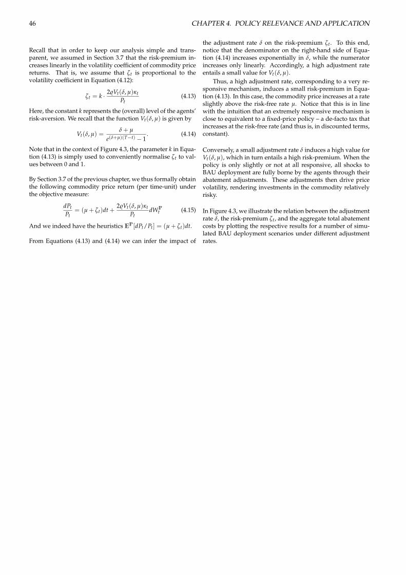
46 CHAPTER 4. POLICY RELEVANCE AND APPLICATION
Recall that in order to keep our analysis simple and trans-parent, we assumed in Section 3.7 that the risk-premium in-creases linearly in the volatility coefficient of commodity pricereturns. That is, we assume that zt is proportional to thevolatility coefficient in Equation (4.12):
zt = k ¨ 2$Vt(d, µ)ktPt
(4.13)
Here, the constant k represents the (overall) level of the agents’risk-aversion. We recall that the function Vt(d, µ) is given by
Vt(d, µ) =d + µ
e(d+µ)(T´t) ´ 1. (4.14)
Note that in the context of Figure 4.3, the parameter k in Equa-tion (4.13) is simply used to conveniently normalise zt to val-ues between 0 and 1.
By Section 3.7 of the previous chapter, we thus formally obtainthe following commodity price return (per time-unit) underthe objective measure:
dPtPt
= (µ + zt)dt +2$Vt(d, µ)kt
PtdWP
t (4.15)
And we indeed have the heuristics EP [dPt/Pt] = (µ + zt)dt.
From Equations (4.13) and (4.14) we can infer the impact of
the adjustment rate d on the risk-premium zt. To this end,notice that the denominator on the right-hand side of Equa-tion (4.14) increases exponentially in d, while the numeratorincreases only linearly. Accordingly, a high adjustment rateentails a small value for Vt(d, µ).
Thus, a high adjustment rate, corresponding to a very re-sponsive mechanism, induces a small risk-premium in Equa-tion (4.13). In this case, the commodity price increases at a rateslightly above the risk-free rate µ. Notice that this is in linewith the intuition that an extremely responsive mechanism isclose to equivalent to a fixed-price policy – a de-facto tax thatincreases at the risk-free rate (and thus is, in discounted terms,constant).
Conversely, a small adjustment rate d induces a high value forVt(d, µ), which in turn entails a high risk-premium. When thepolicy is only slightly or not at all responsive, all shocks toBAU deployment are fully borne by the agents through theirabatement adjustments. These adjustments then drive pricevolatility, rendering investments in the commodity relativelyrisky.
In Figure 4.3, we illustrate the relation between the adjustmentrate d, the risk-premium zt, and the aggregate total abatementcosts by plotting the respective results for a number of simu-lated BAU deployment scenarios under different adjustmentrates.
4.4. CONCLUSIONS 47
Realised Total Aggregate Abatement Costs versus Risk-Premia for Different Adjustment Rates
Risk Premium
Aggr
egat
e C
ompl
ianc
e C
osts
/=0/year
/=0.05/year
/=0.1/year
/=0.2/year
/=0.5/year
/=0.75/year
/=1/year
Figure 4.3: Realised total aggregate abatement costs and risk-premia for 500 simulated BAU deploymentpaths under different adjustment rates in a discretised setting; obtained for an initial bank of B0 = 2Bn units,an expected BAU deployment of 2Bn units per time-unit and a constant allocation of 250Mn units per time-unit; the standard deviation in BAU deployment is 200Mn units per time-unit, and c = 0. The time horizonis set to 30 time-units. Abatement costs are parameterised by Q0 = 5 Euros/unit and $ = 0.25 Euros persquared unit. The risk-free interest rate is µ = 3%. The figure shows a scatterplot on a logarithmic scaleon both axes, where both dimensions are normalised to values between 0 and 1.
We simulate 500 BAU deployment paths on a discretised time-grid, in order to illustrate the impact of d on risk-premiaand costs. Each dot in Figure 4.3 represents the outcomeof one simulation, where we selected seven different adjust-ment rates to illustrate the effect of the mechanism across thepolicy spectrum. The adjustment rate increases from d = 0(with respective results appearing in light grey in the upperright-corner) to 100% per time-unit6 (with results appearingin dark grey towards the left-hand side of the Figure). Therealised aggregate abatement costs (vertical axis) and risk-premia (horizontal axis) for each adjustment rate can be iden-tified as distinct clouds of scattered points across the figure,highlighted in different shadings. Note that the figure showsa plot with logarithmic scales on both axes. Accordingly, theresults for lower adjustment rates are scattered farther apartthan for higher adjustment rates, which corresponds to thefact that the variability in risk-premia and compliance costsdiminishes with increasing responsiveness.
Figure 4.3 confirms our previous intuition behind the decom-position of total aggregate abatement costs: The riskiness ofinvesting in the commodity decreases monotonically with anincreasing responsiveness. Accordingly, the cost of adjusting
to shocks on behalf of the agents is reduced when increasingd. However, this increase in responsiveness comes at the costof thinning out the profitability of inter-temporal cost-savingopportunities, and, in this example, an overall decreased cap.In this example we see that, beyond an adjustment rate ofabout 20% per time-unit, these effects override the benefitsassociated to the reduced uncertainty regarding the expectedabatement requirement.
4.4 Conclusions
By means of our generic responsive mechanism, we examineda spectrum of policies between a pure quantity instrument(such as emissions trading systems with a fixed cap) on theone hand, and pure price instruments (such as fixed taxes orfixed tax trajectories) on the other hand. Each point on thepolicy spectrum is characterised by a level of cap stringency,i.e. the degree of liberty by which the regulator allows thecap to respond to changes in the system due to shocks in thecommodity demand. We made this characterisation possibleby employing an adjustment rate d, which parameterises thestrength of the regulatory response. In that sense, this parame-ter d represents the converse notion to cap stringency, since the
6Note that in the discretised setting, allocation adjustments at each point in time are effective only at the respective next point in time.Hence, even for an adjustment rate of 100% per time-unit, some uncertainty remains.

48 CHAPTER 4. POLICY RELEVANCE AND APPLICATION
determination to carry out strong responses may require sub-stantial deviations from the ex-ante cap, whereas respondingonly weakly tends to require only minor deviations.
The system dynamics, which are subject to both uncertaintyand the responsive mechanism, depend upon the reciprocalresponses from the market and the regulator through time.Since the agents’ optimisation problem depends on the ex-pected future development of the system state, the problemof finding the equilibrium dynamics is subject to the com-plexities of solving the above reciprocity. In particular, when
agents are risk-averse, the stochastic behaviour of the entiresystem becomes an intriguing topic. In the present work, wesolved this inter-dependency and obtained the system’s Q-strong equilibrium dynamics in closed form. With the pricedynamics readily available, we then show that the obtainedequilibrium is also P-weak, and the risk-premia obtained un-der an exemplary linearity assumption (with respect to thefunctional representation of risk-aversion) are obtained as aby-product. Finally, we demonstrated that by choosing anoptimal adjustment rate, the regulator can maximise the cost-efficiency of the system in a stochastic setup.
Bibliography
[Bain, 1948] Bain, J. S. (1948). Output quotas in imperfect cartels. The Quarterly Journal of Economics, 62(4):617–622.
[Bertsekas and Shreve, 1978] Bertsekas, D. P. and Shreve, S. E. (1978). Stochastic optimal control: The discrete time case, volume 23.Academic Press New York.
[Doda, 2016] Doda, B. (2016). How to price carbon in good times... and bad! WIREs Climate Change, 7(7):135–144.
[Ellerman et al., 2015a] Ellerman, D., Valero, V., and Zaklan, A. (2015a). An analysis of allowance banking in the EU ETS. EUIWorking Paper RSCAS 2015/29.
[Ellerman et al., 2015b] Ellerman, D., Valero, V., and Zaklan, A. (2015b). An Analysis of Allowance Banking in the EU ETS.EUI Working Paper RSCAS 2015/29.
[Ellerman and Wing, 2003] Ellerman, D. and Wing, I. (2003). Absolute Versus Intensity-Based Emission Caps. Climate Policy,3(1):7–20.
[Fell, 2015] Fell, H. (2015). Comparing Policies to Confront Permit Over-allocation. Unpublished working paper.
[Fell and Morgenstern, 2010] Fell, H. and Morgenstern, R. (2010). Alternative Approaches to Cost Containment in a Cap-and-Trade System. Environmental and Resource Economics, 47(2):275–297.
[Fell et al., 2012] Fell, H., Morgenstern, R., and Palmer, K. (2012). Soft and hard price collars in a cap-and-trade system: Acomparative analysis. Journal of Environmental Economics and Management, 64:183–198.
[Frino et al., 2010] Frino, A., Kruk, J., and Lepone, A. (2010). Liquidity and Transaction Costs in the European Carbon FuturesMarket. Journal of Derivatives and Hedge Funds, 16(2):100–115.
[Golosov et al., 2014] Golosov, M., Hasslet, J., Krussell, P., and Tsyvinski, A. (2014). Optimal Taxes on Fossil Fuel in GeneralEquilibrium. Econometrica, 82:41–88.
[Grafton, 1996] Grafton, R. Q. (1996). Individual transferable quotas: theory and practice. Reviews in Fish Biology and Fisheries,6(1):5–20.
[Grosjean et al., 2014] Grosjean, G., Acworth, W., Flachsland, C., and Marschinski, R. (2014). After monetary policy, climatepolicy: is delegation the key to EU ETS reform? Climate Policy, 1:1–25.
[Grull and Taschini, 2011] Grull, G. and Taschini, L. (2011). Cap-and-Trade Properties under Different Hybrid Scheme designs.Journal of Environmental Economics and Management, 61(1):107–118.
[Hartley and Hartley, 2002] Hartley, J. E. and Hartley, J. E. (2002). The representative agent in macroeconomics. Routledge.
[Hepburn, 2006] Hepburn, C. (2006). Regulation by Prices, Quantities, or Both: A Review of Instrument Choice. Oxford Reviewof Economic Policy, 22(2):226–247.
[Heutel, 2012] Heutel, G. (2012). How should environmental policy respond to business cycles? Optimal policy under persis-tent productivity shocks. Review of Economic Dynamics, 15:244–264.
[Hotelling, 1931] Hotelling, H. (1931). The economics of exhaustible resources. Journal of political Economy, 39(2):137–175.
[Jotzo and Pezzey, 2007] Jotzo, F. and Pezzey, J. (2007). Optimal intensity targets for greenhouse gas emissions trading underuncertainty. Environmental and Resource Economics, 38(2):259–284.
[Kollenberg and Taschini, 2016a] Kollenberg, S. and Taschini, L. (2016a). Dynamic supply adjustment and banking underuncertainty: The market stability reserve. Available at SSRN.
[Kollenberg and Taschini, 2016b] Kollenberg, S. and Taschini, L. (2016b). Emissions trading systems with cap adjustments.Journal of Environmental Economics and Management, 80:20–36.
[Krylov, 2008] Krylov, N. V. (2008). Controlled diffusion processes, volume 14. Springer Science & Business Media.
[Landis, 2015] Landis, F. (2015). Interpolation of Abatement Cost According to PACE. Unpublished working paper.
[Medina et al., 2014] Medina, V., Pardo, A., and Pascual, R. (2014). The Timeline of Trading Frictions in the European CarbonMarket. Energy Economics, 42(3):378–394.
[Newell and Pizer, 2008] Newell, R. G. and Pizer, W. A. (2008). Regulating Stock Externalities under Uncertainty. Journal ofEnvironmental Economics and Management, 56:221–233.
[Perino and Willner, 2015] Perino, G. and Willner, M. (2015). The Price and Emission Effects of a Market Stability Reserve in aCompetitive Allowance Market. WiSo-HH Working Paper Series, No. 28.
49
50 BIBLIOGRAPHY
[Pham, 2009] Pham, H. (2009). Continuous-time stochastic control and optimization with financial applications, volume 61. SpringerScience & Business Media.
[Pizer, 2002] Pizer, W. A. (2002). Combining Price And Quantity Controls To Mitigate Global Climate Change. Journal of PublicEconomics, 85:409–434.
[Poundstone, 1992] Poundstone, W. (1992). Prisoner’s dilemma: John von neuman, game theory, and the puzzle of the bomb.
[Roberts and Spence, 1976] Roberts, M. J. and Spence, M. (1976). Effluent charges and licenses under uncertainty. Journal ofPublic Economics, 5(3):193–208.
[Rubin, 1996] Rubin, J. D. (1996). A model of intertemporal emission trading, banking, and borrowing. Journal of EnvironmentalEconomics and Management, 31:269–286.
[Schennach, 2000] Schennach, S. M. (2000). The economics of pollution permit banking in the context of title iv of the 1990clean air act amendments. Journal of Environmental Economics and Management, 40:189–210.
[Teeguarden, 1969] Teeguarden, D. E. (1969). Allocating public timber by transferable purchasing quotas: A policy analysis.Natural Resources Journal, 9(4):576–589.
[The European Commission, 2012] The European Commission (2012). Report from the Commission to the European Parlia-ment and the Council: The state of the European carbon market in 2012 . Technical report, The European Commission,Brussels.
[The European Parliament and Council, 2015] The European Parliament and Council (2015). Decision (EU) 2015/1814 of theEuropean Parliament and of the Council of 6 October 2015 concerning the establishment and operation of a market stabilityreserve for the Union greenhouse gas emission trading scheme and amending Directive 2003/87/EC.
[Unold and Requate, 2001] Unold, W. and Requate, T. (2001). Pollution control by options trading. Economics Letters, 73:353–358.
[Weitzman, 1974] Weitzman, M. L. (1974). Prices vs. Quantities. Review of Economic Studies, 41(4):683–691.