228

NATIONAL COOPERATIVE HIGHWAY RESEARCH PROGRAM REPORT 228

CALIBRATION OF RESPONSE-TYPE ROAD ROUGHNESS

MEASURING SYSTEMS

/

TRANSPORTATION RESEARCH BOARD NATIONAL RESEARCH COUNCIL

[ Idaho Transportation Department

L_RESEARCH LIBRARY

TRANSPORTATION RESEARCH BOARD 1980

Officers

CHARLEY V. WOOTAN, Chairman THOMAS D. LARSON, Vice Chairman

THOMAS B. DEEN, Executive Director

Executive Committee

LANGHORNE M. BOND, Federal Aviation Administrator, U.S. Department of Transportation (ex officio) FRANCIS B. FRANCOIS, Executive Director, American Assn. of State Highway and Transportation Officials (ex officio) WILLIAM J. HARRIS, JR., Vice President (Res. and Test Dept.), Association of American Railroads (ex officio) JOHN S. HASSELL, JR., Federal Highway Administrator, U.S. Department of Transportation (ex officio) PETER G. KOLTNOW, President, Highway Users Federation for Safety and Mobility (ex officio, Past Chairman 1979) A. SCHEFFER LANG, Consultant, Washington, D.C. (ex officio, Past Chairman 1978) THEODORE C. LUTZ, Urban Mass Transportation Administrator, U.S. Department of Transportation (ex officio) ELLIOTT W. MONTROLL, Chairman, Commission on Sociotechnical Systems, National Research Council (ex officio) JOHN M. SULLIVAN, Federal Railroad Administrator, U.S. Department of Transportation (ex officio) JOHN F. WING, Senior Vice President, Boo; Allen & Hamilton, Inc. (ex officio, MTRB liaison) GEORGE J. BEAN, Director of Aviation, Hillsborough County (Florida) Aviation Authority RICHARD P. BRAUN, Commissioner, Minnesota Department of Transportation LAWRENCE D. DAHMS, Executive Director, Metropolitan Transportation Commission, San Francisco Bay Area ARTHUR C. FORD, Assistant Vice President (Long-Range Planning), Delta Air Lines ADRIANA GIANTURCO, Director, California Department of Transportation WILLIAM C. HENNESSY, Commissioner, New York State Department of Transportation ARTHUR J. HOLLAND, Mayor, City of Trenton, N.J. JACK KINSTLINGER, Executive Director, Colorado Department of Highways THOMAS D. LARSON, Secretary, Pennsylvania Department of Transportation MARVIN L. MANHEIM, Professor of Civil Engineering, Massachusetts Institute of Technology DARRELL V MANNING, Director, Idaho Transportation Department THOMAS D. MORELAND, Commissioner and State Highway Engineer, Georgia Department of Transportation DANIEL MURPHY, County Executive, Oakland County Courthouse, Michigan RICHARD S. PAGE, General Manager, Washington (D.C.) Metropolitan Area Transit Authority PHILIP J. RINGO, Chairman of the Board, ATE Management & Service Co., Inc. MARK D. ROBESON, Chairman, Finance Committee, Yellow Freight Systems, inc. GUERDON S. SINES, Vice President (In formation and Control Systems) Missouri Pacific Railroad WILLIAM K. SMITH, Vice President (Transportation), General Mills, Inc. JOHN R. TABB, Director, Mississippi State Highway Department CHARLEY V. WOOTAN, Director, Texas Transportation Institute, Texas A&M University

NATIONAL COOPERATIVE HIGHWAY RESEARCH PROGRAM

Transportation Research Board Executive Committee Subcommittee for the NCHRP

CHARLEY V. WOOTAN, Texas A&M University (Chairman) JOHN S. HASSELL, JR., U.S. Dept. of Transp. THOMAS D. LARSON, Pennsylvania Dept. of Transportation ELLIOTT W. MONTROLL, National Research Council FRANCIS B. FRANCOIS, Amer. Assn. of State Hwy. and Transp. Officials PETER G. KOLTNOW, Hwy. Users Fed, for Safety & Mobility

THOMAS B. DEEN, Transportation Research Board

Field of Design Area of Pavements Project Panel, CI-18

ROLANDS L. RIZENBERGS, Kentucky Dept. of Transp. (Chairman) WOUTER GULDEN, Georgia Dept. of Transportation VERNON J. MARKS, Iowa Dept. of Transportation W. E. MEYER, The Pepinsylvania State Univ. FREDDY L. ROBERTS, ARE inc—Engineering Consultants

Program Stag

KRIEGER W. HENDERSON, JR., Director LOUIS M. MAcGREGOR, Administrative Engineer CRAWFORD F. JENCKS, Projects Engineer R. IAN KINGHAM, Projects Engineer

FREDERIC R. ROSS, Wisconsin Dept. of Transportation PAUL N. SONNENBURG, Construction Eng. Research Lab. ELSON B. SPANGLER, Consultant RUDOLPH R. HEGMON, Federal Highway Administration L. F. SPAINE, Transportation Research Board

ROBERT J. REILLY, Projects Engineer HARRY A. SMITH, Projects Engineer ROBERT E. SPICHER, Projects Engineer HELEN MACK, Editor

bi

NATIONAL COOPERATIVE HIGHWAY RESEARCH PROGRAM 228 REPORT

CALIBRATION OF RESPONSE-TYPE ROAD ROUGHNESS

MEASURING SYSTEMS

T. D. GILLESPIE, M. W. SAYERS, AND L SEGEL University of Michigan

Ann Arbor, Michigan

RESEARCH SPONSORED BY THE AMERICAN ASSOCIATION OF STATE HIGHWAY AND

TRANSPORTATION OFFICIALS IN COOPERATION I WITH THE FEDERAL HIGHWAY ADMINISTRATION

AREAS OF INTEREST:

PAVEMENT DESIGN AND PERFORMANCE

MAINTENANCE (HIGHWAY TRANSPORTATION)

TRANSPORTATION RESEARCH BOARD NATIONAL RESEARCH COUNCIL

WASHINGTON, D.C. DECEMBER 1980

NATIONAL COOPERATIVE HIGHWAY RESEARCH PROGRAM

Systematic, well-designed research provides the most ef-fective approach to the solution of many problems facing highway administrators and engineers. Often, highway problems are of local interest and can best be studied by highway departments individually or in cooperation with their state universities and others. However, the accelerat-ing growth of highway transportation develops increasingly complex problems of wide interest to highway authorities. These problems are best studied through a coordinated program of cooperative research. In recognition of these needs, the highway administrators of the American Association of State Highway and Trans-portation Officials initiated in 1962 an objective national highway research program employing modern scientific techniques. This program is supported on a continuing basis by funds from participating member states of the Association and it receives the full cooperation and support of the Federal Highway Administration, United States Department of Transportation. The Transportation Research Board of the National Re-search Council was requested by the Association to admin--ister --the- research --program -because of the Board's- recog-nized objectivity and understanding of modern research practices. The Board is uniquely suited for this purpose as: it maintains an extensive committee structure from which authorities on any highway transportation subject may be drawn; it possesses avenues of communications and cooperation with federal, state, and local governmental agencies, universities, and industry; its relationship to its parent organization, the National Academy of Sciences, a private, nonprofit institution, is an insurance of objectivity; it maintains a full-time research correlation staff of special-ists in highway transportation matters to bring the findings of research directly to those who are in a position to use them.

The program is developed on the basis of research needs identified by chief administrators of the highway and trans-portation departments and by committees of AASHTO. Each year, specific areas of research needs to be included in the program are proposed to the Academy and the Board by the American Association of State Highway and Trans-portation Officials. Research projects to fulfill these needs are defined by the Board, and qualified research agencies are selected from those that have submitted proposals. Ad-ministration and surveillance of research contracts are responsibilities of the Academy and its Transportation Research Board.

The needs for highway research are many, and the National Cooperative Highway Research Prograni can make signifi-cant contributions to the solution of highway transportation problems of mutual concern to many responsible groups. The program, however, is intended to complement rather than to substitute for or duplicate other highway research programs.

NCHRP Report 228

Project 1-18 FY '77

ISSN 0077-5614 ISBN 0-309-03034-X

L. C. Catalog Card No. 80-54 193

Price: $7.60

Notice

The project that is the subject of this report was a part of -the National Cooperative Highway Research Program conducted by the Transportation Research Board with the approval of the Governing Board of the National Research Council, acting in behalf of the National Academy of Sciences. Such approval reflects the Governing Board's judgment that the program concerned is of national impor-tance and appropriate with respect to both the purposes and re-sources of the National Research Council. - The members of the technical committee selected to monitor this project and to review this report were chosen for recognized scholarly competence and with due consideration for the balance of disciplines appropriate to the project. The opinions and con-clusions expressed or implied are those of the research agency that performed the research, and, while they have been accepted as appropriate by the technical committee, they are not necessarily those

- of the =Transportation Research--Board, the-National Research Coun- - cil, the National Academy of Sciences, or the program sponsors. Each report is reviewed and processed according to procedures established and monitored by the Report Review Committee of the National Academy of Sciences. Distribution of the report is ap-proved by the President of the Academy upon satisfactory comple- tion of the review process. - The National Research Council was established by the National Academy of Sciences in 1916 to associate the broad community of science and technology with the Academy's purposes of furthering knowledge and of advising - the federal government. The Council operates in accordance with _general policies determined by the Academy under the authority of its Congressional charter of 1863, which establishes the Academy as a private, non-profit, self-governing membership corporation. The Council has become the principal operating agency of both the Academy of Sciences and the National Academy of Engineering in the conduct of their services to the gov-ernment, the public, and the scientific and engineering communities. It is administered jointly by both Academies and the Institute of Medicine. The Academy of Engineering and the Institute of Medicine were established in 1964 and 1970, respectively, under the charter of the Academy of Sciences. The Transportation Research Board evolved from the 54-year-old Highway Research Board. The TRB incorporates all former HRB activities but also performs additional functions under a broader scope involving all modes of transportation and the interactions of transportation with society.

Published reports of the

NATIONAL COOPERATIVE HIGHWAY RESEARCH PROGRAM

are available from:

Transportation Research Board National Academy of Sciences 2101 Constitution Avenue, N.W. Washington, D.C. 20418

Printed in the United States of America.

FOREWORD This report contains the results of an intensive study of response-type road

- roughness measuring systems (primarily Mays- and PCA-type road meters) for the

By Staff purpose of developing calibration and correlation procedures. An artificial road

Transportation bump approach is described as a simplified method for a calibration check of road

Research Board meter systems. This method offers potential for calibrating systems over the moderate-to-rough range of the roughness scale. Currently available road meters are not generally suitable for assessing the roughness (smoothness) of newly con-structed roads. The findings of this study will be of particular interest to highway and airport personnel responsible for collection and analysis of data on pavement sUrface characteristics, pavement rehabilitation and management programs, and

testing and research activities.

Road roughness measuring systems used by many state highway and transpor-tation agencies are of the type that accumulate the displacement measurement between the rear axle housing and the body of the vehicle in which the instrument is mounted. The main advantages of these response-type systems are their relatively low cost, simplicity of operation, and high measuring speed. However, the measure-ments are influenced by the characteristics of the host vehicle. Time stability, cali-bration, and correlation with other similar and dissimilar systems are problems. The objective of this research was the development and verification of relatively rapid and inexpensive methods for the calibration and correlation of response-type road roughness measuring systems.

The research approach adopted by the University of Michigan's project staff included ( 1 ) a functional analysis of the components of a typical measurement sys-tem, (2) a dynamic analysis of the study measurement system (a vehicle contain-ing two response-type measuring instruments) mounted on a hydraulic road simu-lator, (3) field tests on local road sections with various degrees of roughness, (4) the development of an artificial road bump method for calibration, and (5) a

field evaluation of the artificial road bump calibration method. It was found that different response-type roughness measurement systems measure different roughness statistics (the combination of the amplitude and frequency of the recorded vertical displacement). The measurement instruments often exhibit hysteresis effects. The vehicles in which the instruments are installed contribute to the variation in measure-ments due to shock absorber type and condition, tire pressure, tire/wheel non-

uniformities, and weight changes. The diverse types of road roughness measuring systems (Mays roadmeter, PCA

roadmeter, CHLOE, BPR roughometer, and GMR-type profilometer) each mea-sure qualities of a surface that constitute different aspects of road roughness. Although these systems provide measurements that can be related to each other, comparison of measurements between users is not meaningful. This report con-tains recommendations for adoption of a national measurement scale for road rough-ness. To improve the calibration of measurement systems containing Mays- and PCA-type meters, the report recommends the following with regard to the host vehicle: (1) use of heavy-duty shock absorbers, (2) regular balancing of rear tire and wheel assemblies, and (3) maintenance of tire pressures within 1 psi (hot) when making measurements. The system should be operated at mean traffic speed during measurements. Primary calibration of the systems should be by correlation with roughness computed from a road profile, but the artificial road bump approach can be used as a simplified calibration check.

This report.provides individual highway and transportation agencies with rec-ommendations for calibrating road roughness measuring systems to maintain year-to-year continuity in measurement data and to standardize measurements from their different systems. Further research is recommended to improve comparability of measurements between agencies and to relate roughness measurements to pavement serviceability.

CONTENTS

1 SUMMARY

PARTI

2 CHAPTER ONE Introduction and Research Approach Problem Statement and Objectives Scope Research Approach

6 CHAPTER TWO Findings Theory of Operation RTRRM System Variable Sensitivities Evaluation of Calibration Methods

31 CHAPTER THREE Application of Research Results Pavement Serviceability Correlations Calibration Uses of RTRRM Systems Future Improvements to RTRRM Systems

38 CHAPTER FOUR Conclusions and Recommendations Conclusions and Recommendations Related to Current

Practice Conclusions and Recommendations Related to Future

Improvements

41 REFERENCES

PART II

42 APPENDIX A RTRRM System Calibration Methods

55 APPENDIX B Correlation Program

64 APPENDIX C Theory of Operation of Road Roughness Measur- ing Systems

75 APPENDIX 0 Dynamic Tests at the U.S. Army. Tank Auto-motive Research and Development Command

ACKNOWLEDGMENTS

/

The research reported herein was performed under NCHRP Project 1-18 by the Highway Safety Research Institute, The University of Michigan. Dr. Thomas D. Gillespie, Associate Research Scientist, served as the Principal Investigator. Pro-fessor Leonard Segel, Head of the Physical Factors Division, served as Project Director.

The work was done under the general supervision of Dr. Gillespie. Mr. Michael Sayers, Research Associate, performed most of the analysis and computer simulation and is a co-author of the report. Assistance in the experimental testing was ob-tained from Mr. Doug Brown, Engineer II, and from the Insti-tute's engineering shop facilities supervised by Mr. Joseph Bois-sonneault. Assistance in the general administrative operations of the project was provided by Ms. Jeannette Nafe.

The Michigan Department of Transportation, under a sub-contract arrangement, provided technical support through the services of Mr. John Darlington and Mr. Leo DeFrain, and the use of the Rapid Travel Profilometer. The U.S. Army Tank Automotive Research and Development Command, also under subcontract, provided use of their hydraulic road simulator fa-cilities coordinated through Dr. Richard Lee.

Finally, assistance was received from the Georgia Department of Transportation, Kentucky Department of Transportation, Ohio Department of Transportation, West Virginia Department of Highways, and K. J. Law Engineers, Inc., in the conduct of. a Correlation Program with road roughness measuring systems.

CALIBRATION OF RESPONSE-TYPE ROAD ROUGHNESS MEASURING SYSTEMS

SUMMARY The use of response-type road roughness measuring systems (RTRRM sys- tems) for road roughness surveys is complicated by a lack of understanding of their measurement function and means for calibration to obtain measurements with definable accuracy and consistency. The research conducted under NCHRP Project 1718 was directed toward answering those needs.

Analysis of Mays- and PCA-meter-based systems and comparison against other road roughness measurement systems show that they measure different characteristics of road roughness. The correlation among the diverse systems is a measure of the correlation between the different road roughness spectral charac-teristics. The simple measure of accrued axle-body motion on which the inches/ mile (I/M) statistic is based is the recommended roughness measure because of its relationship to serviceability and minimal sensitivity to vehicle variables. A more direct version of the I/M statistic, the average rectified velocity (ARV), is recommended, as the appropriate measure of this motIon on RTRRM systems. The ARV is a direct measure of vehicle response to road roughness regardless of operating speed and can be converted to inches/mile when desired.

Many sources of measurement variation are identified. The road meter instruments exhibit hysteresis and quantization effects, which if eliminated reduce sources of variation. The vehicles in which these meters are installed contribute many potential sources of variation. Rear suspension damping (shock absorber strength), tire pressure, tire/wheel nonuniformities, and vehicle weight changes are major sources of variation that necessitate careful operating and maintenance procedures. Recommended practices in the use of RTRRM systems are pro-vided, but ultimately more precise and frequent calibrations are needed to improve accuracy and consistency.

Various calibration methods were evaluated to identify those that would validly scale on-road measurements. A standards calibration scale was formulated using the ARV roughness measurement derived from a reference RTRRM system with defined dynamic response characteristics. The efforts to identify simple, inexpensive calibration methods—in the nature of simple mechanical tests or auxiliary instrumentation which could be installed temporarily for calibration—proved disappointing. Because of the high degree of nonlinearity in the systems, especially in the road meter instruments, calibration can only be accomplished by means of a full spectrum excitation as occurs on a road. Therefore the most rigorous calibration, designated as the primary method, is obtained by correlation of on-road measurements of an RTRRM system against the standard. The most practical means for obtaining the standard ARV roughness measurement con-sists of measuring the road profiles with an inertial profilometer (GMR-type) and inputting these profiles to a simulation of the reference RTRRM system. This method emerges from the research findings as the logical and inevitable choice once one has systematically identified all the factors that must be accommodated in the calibration process. Thus, the research has paid off in justifying the need

2

for this type of calibration equipment, and in refinement of the method relating to the effects of speed, in the choice of statistic, and in the choice of a reference quarter-car simulation. The primary calibration method and the quality of the standard were evaluated in a "Correlation Program" and found satisfactory. A second method of calibration, which uses road bumps equivalent to two standard roughness levels, was also evaluated. The method proved effective for most of the vehicles participating in the Correlation Program, but some problems remain.

Results obtained with the vehicles used in the Correlation Program show RTRRM systems to be capable of measuring road roughness on the reference ARV (RARV) scale with a nominal accuracy of 10 percent after primary cali-bration. The degradation of that accuracy with time will depend on the specific RTRRM system and the operating care exercised by each user. The limits on accuracy result from random errors due to the individual dynamic characteristics of each system responding to the road. The random error has no serious effect on highway network surveys in which it will average away in the summary sta-tistics describing the highway network condition. However, it does limit the utility of measurements on individual road sections as may be needed for maintenance decisions or evaluating the quality of new construction.

Finally; it is concluded (from the available data) that the measurement of reference ARV with properly calibrated RTRRM systems is related to pavement serviceability. Although the precise relationship is not established, the reference ARV can be used as a standard for the objective measurement of road surface roughness in lieu of the subjective pavement serviceability rating.

Ultimately, it is clear-that even though roughness measurements from RTRRM systems relate to serviceability, the attainable accuracy is not sufficient for many pavement management needs. Hence it is recommended that highway agencies encourage research to better relate pavement serviceability to the specific ampli-tude and wavelength content of road roughness, and encourage development of low-cost profile measurement/processing systems needed for the more precise measurement of the essential road roughness properties.

CHAPTER ONE

INTRODUCTION AND RESEARCH APPROACH

A primary responsibility of state highway departments and transportation agencies is maintenance of the highway surface. This activity is a critical function which by a recent estimate (1) was expected to consume more than $30 billion over a 20-year period. Of the total number of desired surface qualities, road roughness has a strong influence on the judgment of its serviceability by the using public. In the AASHO Road Test, the concept of pavement serviceability was devised as a temporal measure of pave-ment performance (2). In those tests, pavement roughness (quantified as the mean value of the profile slope variance measured by a CHLOE-type profilometer) was found to

be the primary correlate of the present serviceability index (PSI). Today, many state highway departments andtrans-portation agencies measure only road roughness for esti-mating the PSI.

An objective measurement of road roughness can serve several functions:

As a means of monitoring the overall condition of the road network.

As information needed for decisions on allocation of maintenance funds.

As a measure of the quality of new construction. As a historical measure of pavement performance

Display module

that can be used in evaluation of alternate construction designs.

On a national basis, the measurement of road roughness (as an information base for determining the allocation of highway trust funds for resurfacing, rehabilitation, and reconstruction) requires that comparable means be used for assessing surface roughness in the different states.

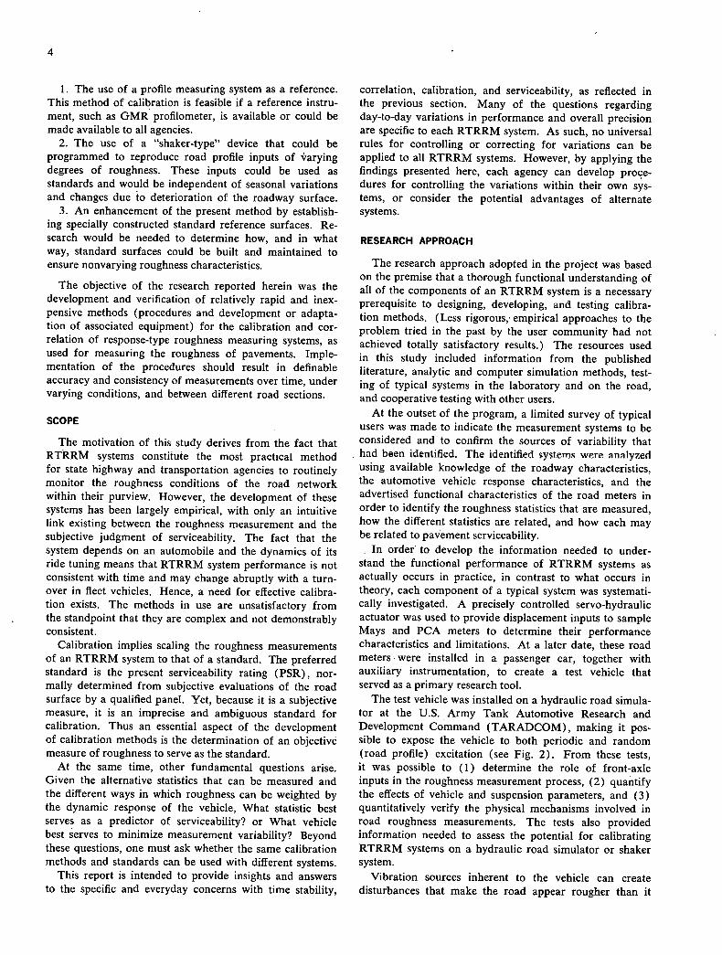
A number of different systems for measuring road roughness have been developed (3). They generally fall into two classes—systems that measure a longitudinal profile characteristic directly, and systems that measure a vehicle's response to the longitudinal profile. The latter type, generally classified as response-type road roughness measure systems (RTRRM systems), include the BPR roughometer (4), the Mays meter (5). and the PCA meter (6). The BPR roughometer is a single-wheel trailer on which an accumulated measure of the displacement of the road wheel relative to the sprung body of the trailer serves to indicate the roughness of the road. The Mays and PCA meters are commercially available instruments (see Fig. 1), which are installed in a conventional passenger car and determine roughness from a measure of the displacement between the rear-axle housing and the body of the auto-mobile.

PROBLEM STATEMENT AND OBJECTIVES

RTRRM systems are used by many state highway and transportation agencies to perform road roughness surveys. The main advantages of these systems are their relatively low cost, simplicity of operation, and high measuring speed. One of their disadvantages is the difficulty of correlating the measurements made by similar and dissimilar systems, and another is their susceptibility to changes that affect their time stability. Most users attempt to minimize the effect of these changes by periodic calibration.

Presently used calibration procedures typically consist of driving the measuring system over roads that have previ-ously been accepted as reference surfaces. The measure-ments obtained are then compared to the roughness values of the reference surfaces. On the basis of these compari-sons, a relationship is obtained which can be applied to measurements on other roads. There are two problems with this calibration method: (I) the roughness values of the reference surfaces are difficult to determine, and (2) once determined, these roughness values change with season, roadway age, and roadway use.

Clearly, there is a need for alternative methods of calibrating RTRRM systems. Some methods that have been suggested are:

Transducer

Optical sensor

\

Cable attached

to axle

PCA meter sanufactured by Soiltest, Inc.

Transducer with optical sensor

Linkage to a

leasured rou;hrmess (i

Strip chart module

tlavs meter

Figure 1. T)vo commercial road meters.

The use of a profile measuring system as a reference. This method of calibration is feasible if a reference instru-ment, such as GMR profilometer, is available or could be made available to all agencies.

The use of a "shaker-type" device that could be programmed to reproduce road profile inputs of ''arying degrees of roughness. These inputs could be used as standards and would be independent of seasonal variations and changes due to deterioration of the roadway surface.

An enhancement of the present method by establish-ing specially constructed standard reference surfaces. Re-search would be needed to determine how, and in what way, standard surfaces could be built and maintained to ensure nonvarying roughness characteristics.

The objective of the research reported herein was the development and verification of relatively rapid and inex-pensive methods (procedures and development or adapta-tion of associated equipment) for the calibration and cor-relation of response-type roughness measuring systems, as used for measuring the roughness of pavements. Imple-mentation of the procedures should result in definable accuracy and consistency of measurements over time, under varying conditions, and between different road sections.

SCOPE

The motivation of this study derives from the fact that RTRRM systems constitute the most practical method for state highway and transportation agencies to routinely monitor the roughness conditions of the road network within their purview. However, the development of these systems has been largely empirical, with only an intuitive link existing between the roughness measurement and the subjective judgment of serviceability. The fact that the system depends on an automobile and the dynamics of its ride tuning means that RTRRM system performance is not consistent with time and may change abruptly with a turn-over in fleet vehicles. Hence, a need for effective calibra-tion exists. The methods in use are unsatisfactory from the standpoint that they are complex and not demonstrably consistent.

Calibration implies scaling the roughness measurements of an RTRRM system to that of a standard. The preferred standard is the present serviceability rating (PSR), nor-mally determined from subjective evaluations of the road surface by a qualified panel. Yet, because it is a subjective measure, it is an imprecise and ambiguous standard for calibration. Thus an essential aspect of the development of calibration methods is the determination of an objective measure of roughness to serve as the standard.

At the same time, other fundamental questions arise. Given the alternative statistics that can be measured and the different ways in which roughness can be weighted by the dynamic response of the vehicle, What statistic best serves as a predictor of serviceability? or What vehicle best serves to minimize measurement variability? Beyond these questions, one must ask whether the same calibration methods and standards can be used with different systems.

This report is intended to provide insights and answers to the specific and everyday concerns with time stability,

correlation, calibration, and serviceability, as reflected in the previous section. Many of the questions regarding day-to-day variations in performance and overall precision are specific to each RTRRM system. As such, no universal rules for controlling or correcting for variations can be applied to all RTRRM systems. However, by applying the findings presented here, each agency can develop proce-dures for controlling the variations within their own sys-tems, or consider the potential advantages of alternate systems.

RESEARCH APPROACH

The research approach adopted in the project was based on the premise that a thorough functional understanding of all of the components of an RTRRM system is a necessary prerequisite to designing, developing, and testing calibra-tion methods. (Less rigorous, empirical approaches to the problem tried in the past by the user community had not achieved totally satisfactory results.) The resources used in this study included information from the published literature, analytic and computer simulation methods, test-ing of typical systems in the laboratory and on the road, and cooperative testing with other users.

At the outset of the program, a limited survey of typical users was made to indicate the measurement systems to be considered and to confirm the sources of variability that had been identified. The identified systems were analyzed using available knowledge of the roadway characteristics, the automotive vehicle response characteristics, and the advertised functional characteristics of the road meters in order to identify the roughness statistics that are measured, how the different statistics are related, and how each may be related to pavement serviceability.

In order to develop the information needed to under-stand the functional performance of RTRRM systems as actually occurs in practice, in contrast to what occurs in theory, each component of a typical system was systemati-cally investigated. A precisely controlled servo-hydraulic actuator was used to provide displacement inputs to sample Mays and PCA meters to determine their performance characteristics and limitations. At a later date, these road meters were installed in a passenger car, together with auxiliary instrumentation, to create a test vehicle that served as a primary research tool.

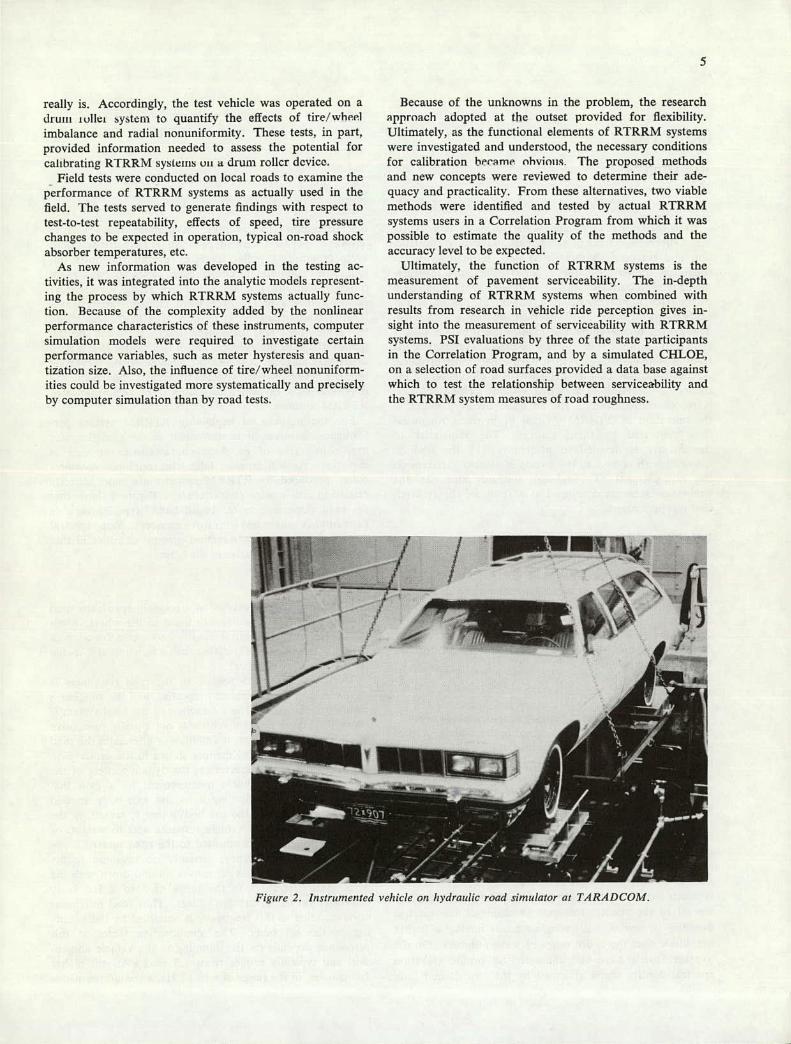
The test vehicle was installed on a hydraulic road simula-tor at the U.S. Army Tank Automotive Research and Development Command (TARADCOM), making it pos-sible to expose the vehicle to both periodic and random (road profile) excitation (see Fig. 2). From these tests, it was possible to (1) determine the role of front-axle inputs in the roughness measurement process, (2) quantify the effects of vehicle and suspension parameters, and (3) quantitatively verify the physical mechanisms involved in road roughness measurements. The tests also provided information needed to assess the potential for calibrating RTRRM systems on a hydraulic road simulator or shaker system.

Vibration sources inherent to the vehicle can create disturbances that make the road appear rougher than it

really is. Accordingly, the test vehicle was operated on a druiii wllei system to quantify the effects of tire/wheel imbalance and radial nonuniformity. These tests, in part, provided information needed to assess the potential for calibrating RTRRM systems on a drum rollcr device. - Field tests were conducted on local roads to examine the

performance of RTRRM systems as actually used in the field. The tests served to generate findings with respect to test-to-test repeatability, effects of speed, tire pressure changes to be expected in operation, typical on-road shock absorber temperatures, etc.

As new information was developed in the testing ac-tivities, it was integrated into the analytic models represent-ing the process by which RTRRM systems actually func-tion. Because of the complexity added by the nonlinear performance characteristics of these instruments, computer simulation models were required to investigate certain performance variables, such as meter hysteresis and quan-tization size. Also, the influence of tire/wheel nonuniform-ities could be investigated more systematically and precisely by computer simulation than by road tests.

Because of the unknowns in the problem, the research approach adopted at the outset provided for flexibility. Ultimately, as the functional elements of RTRRM systems were investigated and understood, the necessary conditions for calibration heeme nhvinns. The proposed methods and new concepts were reviewed to determine their ade-quacy and practicality. From these alternatives, two viable methods were identified and tested by actual RTRRM systems users in a Correlation Program from which it was possible to estimate the quality of the methods and the accuracy level to be expected.

Ultimately, the function of RTRRM systems is the measurement of pavement serviceability. The in-depth understanding of RTRRM systems when combined with results from research in vehicle ride perception gives in-sight into the measurement of serviceability with RTRRM systems. PSI evaluations by three of the state participants in the Correlation Program, and by a simulated CHLOE, on a selection of road surfaces provided a data base against which to test the relationship between serviceability and the RTRRM system measures of road roughness.

JUL- -A- //

lit\

fi

Figure 2. Instrumented vehicle on hydraulic road simulator (it TARA DCOM.

6

CHAPTER TWO

FINDINGS

Response-type road roughness measuring systems repre-sent a diverse spectrum of equipment, in terms of construc-tion and response characteristics and, ultimately, in the roughness numeric obtained. Nevertheless, the measure-ments tend to correlate with serviceability, with a potential existing for improvements in precision by use of proper calibration methods and informed operating personnel. The caliber of the roughness monitoring program in any state and transportation agency is directly related to the level of understanding grasped by the personnel involved. Accordingly, this chapter begins with a discussion of the theory of operation of RTRRM systems. This discussion is recommended reading for all those involved either in the operation of RTRRM systems or in using roughness data generated by these sources. The remainder of the chapter is devoted to presenting (1) the findings obtained with respect to the effects of system variables on the measurement of roughness statistics and (2) the calibration schemes developed as a result -of the research that was performed.

THEORY OF OPERATION

Measurements made by RTRRM systems are the result of the interactions of three basic components—the road, the vehicle, and the road meter instrument. To understand the significance of the measured roughness statistics, the contribution of each component must be known. Appendix C contains the analytic development needed to assess these contributions and the mathematical foundation for the following discussion.

Roads

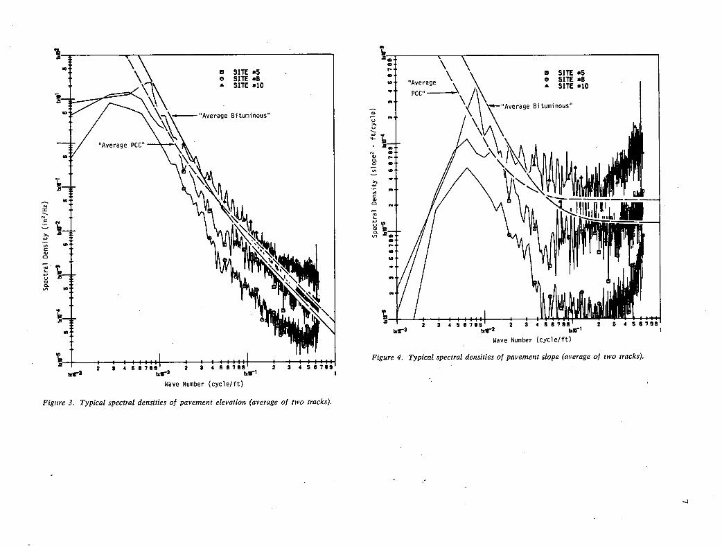
The qualities of a road that affect the perceived rough-ness are almost completely contained in the average vertical profile of the right and left wheel tracks. Because the profile is random in nature, its statistical properties can be conveniently represented by its spectral density. The spectral density is the distribution of profile variance (mean square of elevation = variance when mean elevation = 0) as a function of wave number (where wave number 1 / wavelength, cycle/ft). Roads, like many surfaces, have characteristic trends in the distribution of roughness with wave number. Figure 3 shows spectral densities for a number of different roads. Note that the roughness content is much higher at low wave numbers (long wavelengths) for all of the roads. The general shape of the spectral densities is similar, with rougher roads having a higher amplitude over the entire range of wave numbers. On the average, roads have the characteristic profile elevation spectral density shape indicated by the two dashed lines

that correspond to "average" bituminous roads and to "average" portland cement concrete (PCC) - roads. Both averages are for similar levels of overall roughness, al-though the bituminous construction tends to have more roughness in the low wave number (long wavelength) ranges and less in the high wave number (short wave-length) ranges than the PCC road. The figure 'also shows that none of the real roads have exactly the same spectral density shape as the average, and it is doubtful that a' road exists that perfectly matches the average road. Neverthe-less, the "average" road concept provides a convenient and important basis on which to compare the performance of RTRRM systems.

For the purpose of explaining RTRRM system per-formance, however, it is convenient to think of the road profile in terms of its slope characteristics as well as elevation. As will be seen later, the roughness measure-ments produced by RTRRM systems are more directly related to profile slope characteristics. Figure 4 shows that the road slope is a more "broad band" type of variable (amplitude changes less with wave number). Slope spectral densities are related to elevation spectral densities in that the former is the derivative of the latter.

Vehicle

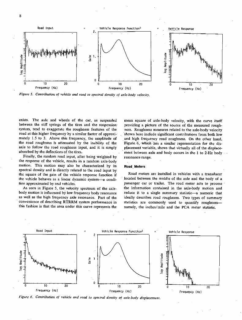
When the road is traversed at a constant speed, the road slope is perceived as a velocity input to the wheel. Simi-larly, the elevation spectral density becomes a function of temporal frequency (Hz) rather than a function of a spatial frequency (wave number).

The response of the vehicle to the road roughness is dependent on speed, vehicle properties, and the roughness content of the road. The interaction of the total system is shown in Figure 5. The vehicle is not equally responsive at all frequencies; rather, it amplifies or attenuates the road excitation in the general manner shown in the center plot. This response plot characterizes the dynamic effect of the vehicle in road roughness measurement by a gain that relates the road profile input to the axle-body motion (rear axle relative to the car body) that is sensed by the road meter. Thus the vehicle response acts to weight, or filter, the roughness transmitted to the road meter.

At very low frequency, virtually no response occurs because the body of the car moves up and down with the axle. At a frequency in the range of 1 to 2 Hz, body resonance on the suspension occurs. Thus road roughness corresponding to this frequency is amplified by the bounc-ing of the car body. The amplification factor at this resonance depends on the damping in the vehicle suspen-sion and typically ranges from 1.5 to 3. At still higher frequencies, in the range of 8 to 12 Hz, a second resonance

bW

Wave Number (cycle/ft)

Figure 3. Typical spectral densities of pavement elevation (average of two tracks).

Average \

PCCfl

C SITE .5 e SITE *8 a SITE .10

Average Bituminous

L11

2 3 4 5 6798 1 2 3 4 5 ties 2 3 4 5 6789'

Wave Number (cycle/ft)

Figure 4. Typical spectral densities of pavement slope (average of two tracks).

= - Vehicle Response

0 =

0

a, 0

Frequency (Hz)

8

Vehicle Response Function2

I OV 0 10 20 0 10 20

Frequency (Hz) Frequency (Hz)

Figure 5. Contribution of vehicle and road to spectral density of axle-body velocity.

Road Input

exists. The axle and wheels of the car, as suspended between the stiff springs of the tires and the suspension system, tend to exaggerate the roughness features of the road at this higher frequency by a similar factor of approxi-mately 1.5 to 3. Above this frequency, the amplitude of the road roughness is attenuated by the inability of the axle to follow the road roughness input, and it is simply absorbed by the deflections of the tires.

Finally, the random road input, after being weighted by the response of the vehicle, results in a random axle-body motion. This motion may also be characterized by its spectral density and is directly related to the road input by the square of the gain of the vehicle response function if the vehicle behaves as a linear dynamic system—a condi-tion approximated by real vehicles;

As seen in Figure 5, the velocity spectrum of the axle-body motion is influenced by low frequency body resonance as well as the high frequency axle resonance. Part of the convenience of describing RTRRM system performance in this fashion is that the area under this curve represents the

mean square of axle-body velocity, with the curve itself providing a picture of the source of the measured rough-ness. Roughness measures related to the axle-body velocity shown here include significant contributions from both low and high frequency road roughness; On the other hand, Figure 6, which has a similar representation for the dis-placement variable, shows that virtually all of the displace-ment between axle and body occurs in the -1 to 2-Hz body resonance range.

Road Meters

Road meters are installed in vehicles with a transducer located between the middle of the axle and the body of a passenger car or trailer. The road. meter acts to process the information contained in the axle-body motion and reduce it to a single summary statistic—a numeric that ideally describes road roughness. Two types of summary statistics are commonly used to quantify roughness—namely, the inches/mile and the PCA meter statistic.

Road Input

2

. 1 10

0

Vehicle Response Function2 Vehicle Response

0 10 20 0 10 20

0 10 20 Frequency (Hz) Frequency (Hz)

Frequency (Hz)

Figure 6. Contribution of vehicle and road to spectral density of axle-body displace,nent.

The inches/mile (I/M) statistic is a measure of accrued axle travel per mile of highway travel, obtained from a displacemenl transducer that detects small increments of axle movement relative to the body. Each increment of movement, whether positive or negative, produces a posi-tive increment of the measured statistic. This is the rough-ness measure normally associated with the Mays meter and BPR roughometer and may be obtained from PCA meters that display the counts accumulated in eah register. The Mays meter (see Fig. 1) advances a strip chart (with a stepper motor) Y64 in. for each detected axle movement of %o in. At the end of a test, the length of the paper that was advanced is multiplied by 6.4, giving inches of axle-body travel. The original BPR roughometer had a ratchet mechanism that advanced a marker when the axle-body travel was positive, but did not move the marker when the axle-body travel was negative. At the end of a test, the marker travel was multiplied by a mechanical scale factor, and then by 2, to account for the unmeasured negative axle travel. The PCA-Wisconsin meter (described in the following in more detail) has a bank of counting registers. Each increment of axle-body motion (typically Ys in.) causes one of the registers to increase its count by one. At the end of the test, the total number of counts may be multiplied by the resolution of the transducer (i.e., Y8 in.) to give the total axle travel. In each case, the inches of axle travel is flOtfiä1ized by dividing by - the length of the test section to give the statistic, I/M. Mathematically, the "true" measure of the I/M statistic (in the absence of nonlinear meter effects) is the average rectified velocity (ARV) of the axle-body motion, multiplied by the time needed to travel 1 mile at the test speed. (In other words, the inches accrued in a mile are proportional to the rate at which axle-body displacement changes.) ARV (and hence the I/M statistic) is proportional to root-meansquare (RMS) axle-body velocity on roads for which the rough-ness is both uniformly distributed along its length (statis-tically stationary) and Gaussian. The spectral density of the axle-body velocity indicates the frequency content of the square of the I/M statistic. From Figure 5 it can be seen that the mean square velocity is contained over the fairly broad frequency range of 1 to 15 Hz. Specifically, about 50 percent of the mean square velocity is in the frequency range of 0 to 4 Hz (body resonance), while the remaining 50 percent derives from frequencies above 4 Hz (axle resonance). On the other hand, 90 percent of the mean square displacement is contained in the narrow frequency range 0 to 1.8 Hz.

The PCA meter statistic (often called the "PCA sum of squares") is a weighted sum of counts with the units of in.2 /mile, or sometimes counts/mile. The PCA-Wisconsin meter is the name of a road meter designed by Brokow (6) of the Portland Cement Association and first used by the State of Wisconsin. The PCA meter, like the other road meters, has a transducer fixed between the vehicle axle and body that detects the position of the axle relative to its equilibrium position. The axle position is identified as being a certain number of increments (typically Y8 in.) from the equilibrium position. The transducer is connected to a bank of counting registers, such that each register is

connected to a different possible position. When the axle moves from one position to an adjacent position, the register associated with the "new" position adds one count. Thus, if the axle moves from —% in. to +Y2 in., one count will be added to the registers —2, —1, 0, 1, 2, 3, and 4. If the axle moves back to —% in., a count will be added to registers 3, 2, 1, 0, —1, —2, and —3. In practice, registers 1 and —1 are often connected to the same counter, as are 2, —2 and all other pairs. The 0 position is then not connected to a register. The PCA meter statistic is calcu-lated as:

1 PCA statistic =d2 i R. (1)

where d equals increment size, D equals distance traveled, i equals register number, N equals number of registers, and Ri equals counts in register i. When the d2 term is omitted, the measure of roughness will have the units counts/mile. During the development of the PCA meter, Brokow (6) showed that when the meter is given a signal that starts at zero, increases to an amplitude A, and then returns to zero, with only one reversal when the displace-ment equals A (a sine wave fits this description), the PCA statistic is equal to A 2. The analysis has often been incor-rectly assumed to apply to the random axle-body motion that OCCuis oii the road, leading to the erroneous conclusion that the PCA meter statistic is proportional to some con-ventional mean-square statistic. However, when the data from a road test accumulated in a PCA meter are reduced according to Eq. 1, the relation between the statistic and the vehicle response is fairly complicated. Under the ideal case when the quantization size is negligible, the actual statistic obtained is a function of the joint probability distribution of the axle-body displacement and velocity. When the excitation is stationary and Gaussian, and axle-body displacement and velocity are uncorrelated, the PCA meter statistic is proportional to the product of RMS axle-body velocity and RMS axle-body displacement. Be-cause of the dependence of the PCA meter statistic on RMS displacement, its statistic is strongly dependent on the low frequency (body resonance) portion of the vehicle frequency response and to the low wave number roughness content of the road.

Comparison of Different Road Roughness Measurement Systems

Different RTRRM systems that measure the same statis-tic use vehicles with similar, but not identical, response characteristics. Thus the axle-body motions generated by different systems are weighted somewhat differently and derive from slightly different portions of the road roughness frequency spectrum. Hence, as a minimum, the agreement between RTRRM systems is limited by the correlation between the road spectral density values at different wave numbers. If all roads had identical spectral characteristics, or all RTRRM systems had identical response character-istics, perfect correlation would be observed. Similar RTRRM systems are expected to have good, but imperfect, correlation because of the differences in their response

10

elicited by the particular roughness characteristics of each road.

On the other hand, RTRRM systems that employ different types of road meters, such as the Mays and PCA meters, are sensitive to different portions of the roughness spectrum that are substantially different, with the result that different types of road meter statistics will correlate more poorly. In addition, the differences between vehicles will have greater impact with meters that produce outputs that depend on different resonance characteristics; there-fore the correlation between different types of RTRRM systems will suffer further. Because the correlation depends on specific response characteristics of the vehicles and the statistical properties of the road roughness, no consistent, universal relationship can be expected. Although some correlation can be observed experimentally, there is no practical method by which the observation can be validly extended to other RTRRM systems or even other road systems.

To compare RTRRM systems with other roughness measuring systems, the response characteristics of the other systems must be known. Appendix C provides analyses of all of the measurement systems discussed next.

BPR Roughometer

As previously noted, the BPR roughometer provides an accrued axle travel, JIM statistic. The main differences between the roughometer and passenger-car-based RTRRM systems measuring the J/M statistic are the following. The frequency response of the BPR trailer can differ substan-tially from that of a normal passenger car. Figure 7 shows these differences in terms of the response function gain for a passenger-car simulation used by HSRI (the plot marked "reference"), along with the gain function exhibited by a BPR roughometer/quarter-car simulation based on a trailer owned by the State of Michigan (7) and the gain

2

KENTUCKT MICII!GRN REFERENCE

as

5al

. I

A

4.00 8.00 1200 l0 ftfl0 2A FREQUENCY (HZ)

Figure 7. Comparison of two stale-owned BPR roughometer si,nulations and reference car.

function for a BPR simulation that is implemented on the Kentucky profilomctcr (8). (Appendix C includes details of the BPR roughometer simulations that define the re-sponse functions shown in the figure.) Another difference stems from the fact that operating speed of the BPR roughometer is 20 mph in contrast to the 50-mph speed normally used for other RTRRM systems. At 50 mph, the 1 to 10-Hz frequency range corresponds to the wave num-ber range of 0.014 to 0.14 cycle/ft (wavelengths of 73 to 7.3 ft/cycle), but at 20 mph the same frequency range corresponds to the wave number range of 0.034 to 0.34 cycle/ft (wavelength of 29 to 2.9 ft/cycle). This effect is presented in Figure 8, which shows response functions plotted as functions of wave number (instead of the more conventional cycles/see) for a number of different systems.

In effect, these differences mean that the BPR rough-ometer, while measuring a similar statistic, derives it from a different part of the road spectrum with a different frequency weighting, as shown in Figure 8. Thus, although on the average the BPR roughometer can be correlated with its closest equivalent, the Mays meter, on individual roads a significant random error will result.

CHLOE Pro fi/ometer

The CHLOE is an absolute measuring device (not a response-type system) that holds an important place in the developiiient of the pavcmcnt serviceability conoopt (9). The measured statistic of the CHLOE is called "slope variance," which is calculated conventionally from a measured approximation of the true slope of the road. The CHLOE measures the difference in angles between a small beam with two wheels, 9 in. apart, and the much longer CHLOE trailer, measuring 25.5 ft in length. In order to eliminate any dynamic phenomena, the CHLOE must be towed at a low speed, typically 2 to 3 mph. The relationship between the slope of the profile and the measured slope can be described by the wave number response function. Figure 8 shows that for the CHLOE, the gain is near 1 for wave numbers between 0.02 and 30 cycle/ft (wavelengths from 50 to 3 ft/cycle). For wave numbers beyond this range, the measurement is smaller than the actual slope of the profile. Overall, the CHLOE measures road slope properties over a much different wave number range and with a much different weighting than is obtained with RTRRM systems.

GMR Pro filometer

The GMR profilometer (10) is a device that has been developed to measure the profile of one or two road tracks at speeds comparable to the speed of highway traffic. A small follower wheel is held in the track being profiled with a load of several hundred pounds. A displacement transducer measures the distance between ground and the vehicle supporting the follower wheel, and an accelerome-ter measures the vertical motion of the body of the vehicle. The profile is obtained by doubly integrating the accele-rometer signal and then subtracting the displacement signal to eliminate vehicle motion from the measurement. The

11

BPR R'METER CRR - KSVEL /

£ CRR - MSDIS I CHLOE

x 141CM DOT

111111 III 2 2 4 S RRR 2 2 4 S 8199 2 3 4 58189

W1VE NUMBER (CYCLE/FT)

Figure 8. Comparison of weighting functions inherent in various road roughness measuring systems.

(I) I-

C',

D

a: >

a: LD

U,

wave number content of the measured profile is limited at the low end, in part, by the difficulties of obtaining a reliable measure of the very low accelerations correspond-ing to long wavelengths. In practice, these low frequency signals are intentionally limited by a high pass filter selected to keep the profile amplitude within the range of. the instrumentation. The high wave number content is limited by the dynamic response of the follower wheel (which typically resonates near 100 Hz) and by the geometric effects of wheel curvature. Even with these limitations, GMR profilometers can measure profiles with accurate wave number content over the range of 0.001 to 1 cycle/ft (wavelengths 1000 to 1 ft/cycle), a range much broader than the range measured by any of the foregoing systems, and much broader than the range that normally affects vehicle ride. No standard exists for processing measured profiles to yield a roughness numeric, but some methods that are in use are as follows:

Spectral densities—Road profile spectral densities are used by the automotive industry and the research com-munity for studying vehicle ride and. vibration. Roads can be rated by fitting the measured spectral density to a model spectral density and using one of the model parameters as the.numeric. Road profile spectral densities are not rou-tinely computed, at present, by state road agencies.

Mean-square (or RMS) statistics—Measured .profiles have been used to calculate mean-square statistics of the elevation or slope. However, the resultant statistics depend strongly on the frequency response of the profilometers and on any filtering done during the data processing. As Figure 3 shows, elevation spectral density increases tre-mendously for low wave numbers. Thus measured mean-square elevations will vary directly with the cut-off frequency of the high pass filter. Figure 4 shows that the

slope spectral density is roughly constant for high wave numbers and increases with very low wave numbers. Therefore, a measured slope variance will also depend on the low frequency cut-off point of the high pass filter, as well as on the upper frequency cut-off point, arising from limitations of the follower wheel. Currently, the Michigan Department of Transportation (MDOT) uses a weighted mean-square elevation as a roughness numeric (11). The profile is filtered by a fourth-order band-pass filter, with cut-off frequencies set to correspond with wave numbers 0.02 and 0.5 cycle/ft (wavelengths 50 to 2 ft) as shown in Figure 8, thus creating a well-defined statistic that is inde-pendent of the measuring system. The statistic is then used to predict a ride quality index based on correlations de-veloped by MDOT in a study that collected road profiles and associated ride ratings.

Simulated RTRRM system measurements—A simu-lated vehicle response to a measured profile can be obtained by implementing a vehicle model, characterized by differ-ential equations, on an analog or digital computer. The simulated vehicle is, of course, constant with time and can be tailored to match any desired dynamic model. The model's response can then be summarized by any desired statistic such as I/M. Kentucky and West Virginia now use a simulated BPR roughometer based on differential equations that correspond to the response function shown in Figure 7 and replotted in Figure 8. West Virginia also has a simulation which employs the vehicle model devel-oped in this research as a reference vehicle to be used as a standard in the calibration of RTRRM systems.

All of the systems described produce a roughness statistic that derives from a weighted wave number range of the total road roughness. Figure 8 shows that not only do the

12

The discussion of RTRRM systems that was just pre-sented assumed "ideal" road meters that employ trans-ducers capable of sensing the axle-body motion exactly. In practice, the transducers used with Mays and PCA meters are not ideal but only follow the gross motion with the signal being modified by various effects as discussed indi-vidually in the following. In order to determine the prop-erties of road meters, three commercial meters were procured for laboratory testing along with a fourth meter (see App. B) which was fabricated at HSRI and is identi-fied in Table 2 as "Electronic." Table 2 summarizes the magnitude of each effect to be discussed in detail below.

Quantization

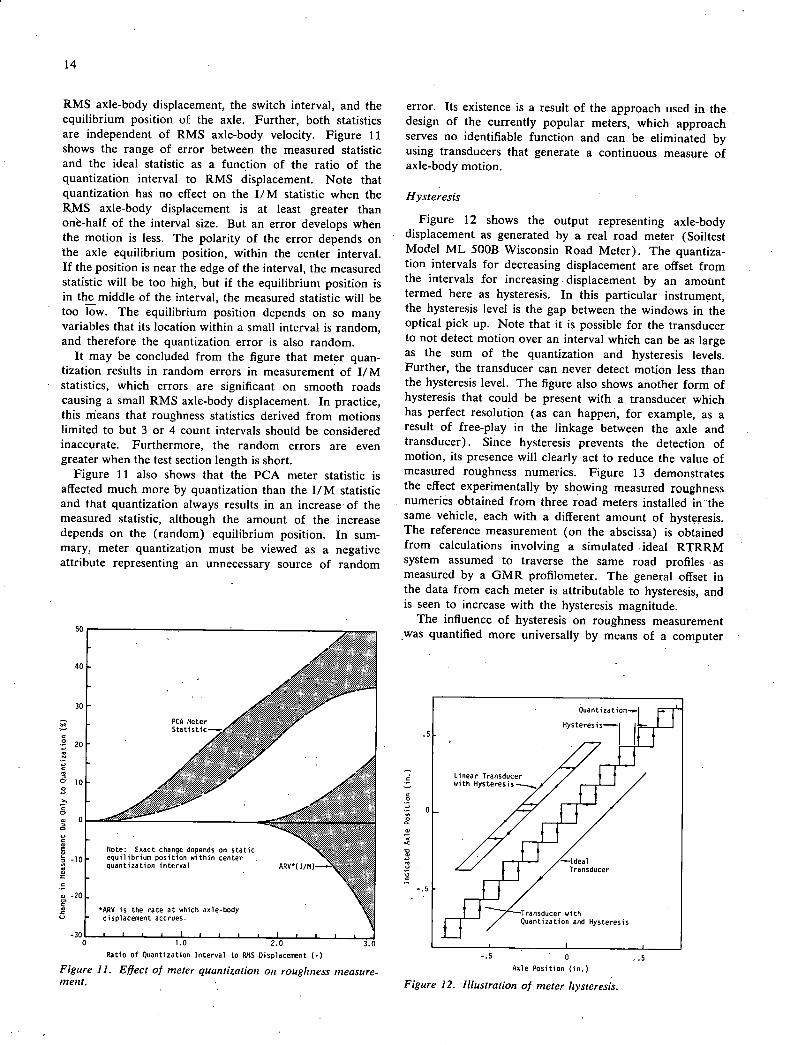
Figure 10 compares the output of an ideal transducer that continuously senses position to that of a transducer which quantizes the position in discrete steps. As shown, the transducer is capable of sensing motion from one interval of position to another, but cannot detect any motion within an interval. Modern road meters usually

RTRRMSYSTEMVARIABLE_SENSITIVITIES detect motion by employing an optical switch that is - triggered by moving an opaque film with rectangui

Understanding the effects of system variables on the windows past a light. The quantization level is then the

measured roughness statistics is necessary both to establish center-to-center distance between the rectangular windows. good procedures for the routine day-to-day use of RTRRM Because the axle-body motion is random, the effect of systems and to understand the role of the calibration quantization on the measurement of roughness numerics process in the use of these systems. The topics covered can be determined by calculating the expected number of here include the important effects deriving froth the road crossings of each of the quantization thresholds, from meters, operating conditions, and vehicles. Special atten- relations used in random signal analysis. The mathematics tion is given to the subject of vehicle damping, because the are contained in Appendix C and show that changes to information presented on this topic provides the basis for both IIM and PCA meter statistics are functions of the

TABLE I

COMPARISON OF DIFFERENT SYSTEM CHARACTERISTICS

System Type Measured Statistic Units of Statistic

Mays Meter, BPR Response Accrued axle travel divided by in/mile roughometer, Unweighted distance traveled (ideal)* sum of PCA meter counts

Profilometer with Absolute Accrued axle travel divided by in/mile simulated RTRRM distance traveled system

PCA meter Response PCA meter statistic (ideal)* in2/mile (or count/mi)

CHLOE Absolute Weighted slope variance slope2

Michigan DOT Absolute Weighted mean-square elevation in2 profilometer -

*Indjcates ideal statistic measured with a perfect meter (i.e., without nonlinearities of hysteresis and quantization).

weighting functions have different shapes, but they often cover different wave number ranges. It can be expected that correlations between measurements taken with the various systems will be poorest for those systems which respond to wave number ranges that overlap the least.

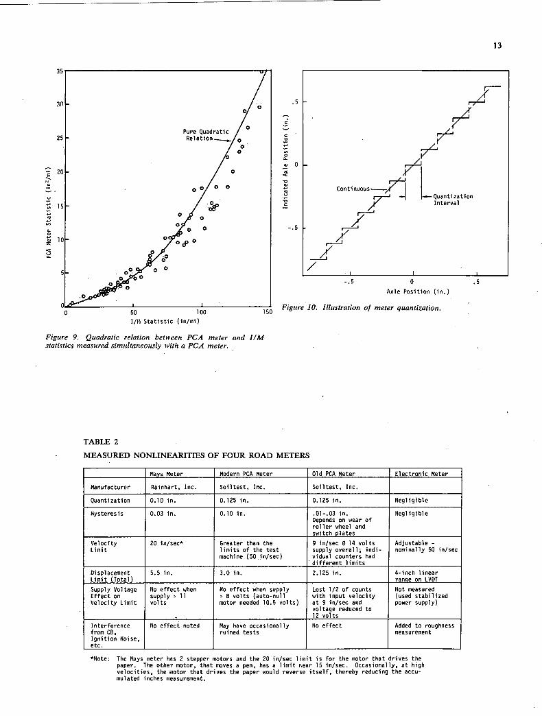
Although Figure 8 illustrates the relative wave number filtering effect associated with each type of roughness measuring system, their comparative performance also depends on the measured statistic obtained from each. Table 1 summarizes the numerics measured by the different systems. The units of the various measures suggest the type of relationship that should be expected between dissimilar systems operated at standard speeds. The PCA meter and CHLOE produce roughness numerics that are average squared measures. They are thus, ideally, linearly related to each other, and quadratically related to the JIM. But because any particular road will have individual peculiari-ties, the relationships between different statistics will be subject to random errors, or scatter. At best, the units of the measurements shown suggest the proper regression form that should be used when experimental correlation between two systems is required. Figure 9 shows the underlying quadratic relation between the JIM and PCA meter statistics. The two types of measurements were both produced by a PCA meter and were made simultaneously.

the recommendations (given later in this report) with respect to the shock absorbers used on vehicles constituting the vehicle part of an RTRRM system.

Road Meter Nonhinearities

Pure Quadratic / 0 Relation ______/

/ 0• /0

/0

oo/"o 0

/.. OJ o

5. /0 cp 0 oI

o oPb 0

.0

2

a

13

0 -5

C

/

7L

Continuous Quantization Interval

/

-.5

-.5 0 .5

Axle Position (in.)

0 50 100 150 Figure 10. Illustration of meter quantizat ion.

I/ti Statistic (in/mi)

Figure 9. Quadratic relation between PCA meter and JIM statistics measured simultaneously with a PCA meter.

TABLE 2

MEASURED NONLINEARITES OF FOUR ROAD METERS

Nays Meter Modern PCA Meter Old PCA Meter Electronic Meter

Manufacturer Rainhart, Inc. Soiltest, Inc. Soiltest, Inc.

Quantization 0.10 in. 0.125 in. 0.125 in. Negligible

Hysteresis 0.03 in. 0.10 in. .Ol-.O3 in. Negligible Depends on wear of roller wheel and switch_plates

Velocity 20 in/sec* Greater than the 9 in/sec @ 14 volts Adjustable - Limit limits of the test supply overall; mdi- nominally 50 in/sec

machine (50 in/sec) vidual counters had different limits

Displacement 5.5 in. 3.0 in. 2.125 in. 4-inch linear Limit (Total) range on LVDT

Supply Voltage No effect when No effect when supply Lost 1/2 of counts Not measured Effect on supply > 11 > 8 volts (auto-null with input velocity (used stabilized Velocity Limit volts motor needed 10.5 volts) at 9 in/sec and power supply)

voltage reduced to 12 volts

Interference No effect noted May have occasionally No effect Added to roughness from CB, ruined tests measurement Ignition Noise, etc.

*Note: The Nays meter has 2 stepper motors and the 20 in/sec limit is for the motor that drives the paper. The other motor, that moves a pen, has a limit rear 15 in/sec. Occasionally, at high velocities, the motor that drives the paper would reverse itself, thereby reducing the accu-mulated inches measurement.

50

40

30

xx

2 20

-30

14

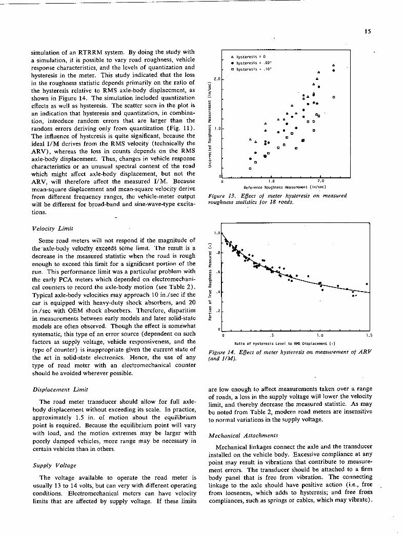
RMS axle-body displacement, the switch interval, and the equilibrium position of the axle. Further, both statistics are independent of RMS axle-body velocity. Figure 11 shows the range of error between the measured statistic and the ideal statistic as a function of the ratio of the quantization interval to RMS displacement. Note that quantization has no effect on the JIM statistic when the RMS axle-body displacement is at least greater than on'e-half of the interval size. But an error develops when the motion is less. The polarity of the error depends on the axle equilibrium position, within the center interval. lithe position is near the edge of the interval, the measured statistic will be too high, but if the equilibrium position is in the middle of the interval, the measured statistic will be too low. The equilibrium position depends on so many variables that its location within a small interval is random, and therefore the quantization error is also random.

It may be concluded from the figure that meter quan-tization results in random errors in measurement of JIM statistics, which errors are significant on smooth roads causing a small RMS axle-body displacement. In practice, this means that roughness statistics derived from motions limited to but 3 or 4 count intervals should be considered inaccurate. Furthermore, the random errors are even greater when the test section length is short.

Figure 11 also shows that the PCA meter statistic is affected much more by quantization than the J/M statistic and that qüantization always results in an increase ofthe measured statistic, although the amount of the increase depends on the (random) equilibrium position. In sum-mary, meter quantization must be viewed as a negative attribute representing an unnecessary source of random

Ratio of Quantization Interval to RMS Displacement (-)

Figure 11. Effect of meter quantization on roughness measure-ment.

error. Its existence is a result of the approach used in the - design of the currently popular meters, which approach serves no identifiable function and can be eliminated by using transducers that generate a continuous measure of axle-body motion.

Hysteresis

Figure 12 shows the output representing axle-body displacement as generated by a real road meter (Soiltest Model ML 500B Wisconsin Road Meter). The quantiza-tion intervals for decreasing displacement are offset from the intervals for increasing displacement by an amount termed here as hysteresis. In this particular instrument, the hysteresis level is the gap between the windows in the optical pick up. Note that it is possible for the transducer to not detect motion over an interval which can be as large as the sum of the quantization and hysteresis levels. Further, the transducer can never detect motion less than the hysteresis level. The figure also shows another form of hysteresis that could be present with a transducer which has perfect resolution (as can happen, for example, as a result of free-play in the linkage between the axle and transducer). Since hysteresis prevents the detection of motion, its presence will clearly act to reduce the value of measured roughness numerics. Figure 13 demonstrates the effect experimentally by showing measured roughness numerics obtained from three road meters installed in the same vehicle, each with a different amount of hysteresis. The reference measurement (on the abscissa) is obtained from calculations involving a simulated ideal RTRRM system assumed to traverse the same road profiles as measured by a GMR profilometer. The general offset in the data from each meter is attributable to hysteresis, and is seen to increase with the hysteresis magnitude.

The influence of hysteresis on roughness measurement was quantified more universally by means of a computer

- Quantization-..-

Hysteresis—1 .5

Linear Transducer with

C 0

0

C- 0 0 C

Ysteresis ,,,,,,//

2 C U Transducer

-.5

ansducer with Quantization and Hysteresis

-.5 0

Axle Position (in.)

Figure 12. Illustration of meter hysteresis.

simulation of an RTRRM system. By doing the study with a simulation, it is possible to vary road roughness, vehicle response characteristics, and the levels of quantization and hysteresis in the meter. This study indicated that the loss in the roughness statistic depends primarily on the ratio of the hysteresis relative to RMS axle-body displacement, as shown in Figure 14. The simulation included quantization effects as well as hysteresis. The scatter seen in the plot is an indication that hysteresis and quantization, in combina-tion, introduce random errors that are larger than the random errors deriving only from quantization (Fig. 11). The influence of hysteresis is quite significant, because the ideal J/M derives from the RMS velocity (technically the ARV), whereas the loss in counts depends on the RMS axle-body displacement. Thus, changes in vehicle response characteristics or an unusual spectral content of the road which might affect axle-body displacement, but not the ARV, will therefore affect the measured JIM. Because mean-square displacement and mean-square velocity derive from different frequency ranges, the vehicle-meter output will be different for broad-band and sine-wave-type excita-tions.

Velocity Limit

Some road meters will not respond if the magnitude of the -axle-body velocity exceeds Omë limit. The result is a decrease in the measured statistic when the road is rough enough to exceed this limit for a significant portion of the run. This performance limit was a particular problem with the early PCA meters which depended on electromechani-cal counters to record the axle-body motion (see Table 2). Typical axle-body velocities may approach 10 in./sec if the car is equipped with heavy-duty shock absorbers, and 20 in/sec with OEM shock absorbers. Therefore, disparities in measurements between early models and later solid-state models are often observed. Though the effect is somewhat systematic, this type of an error source (dependent on such factors as supply voltage, vehicle responsiveness, and the type of counter) is inappropriate given the current state of the art in solid-state electronics. Hence, the use of any type of road meter with an electromechanical counter should be avoided wherever possible.

Displacement Limit

The road meter transducer should allow for full axle-body displacement without exceeding its scale. In practice, approximately 1.5 in. of motion about the equilibrium point is required. Because the equilibrium point will vary with load, and the motion extremes may be larger with poorly damped vehicles, more range may be necessary in certain vehicles than in others.

Supply Voltage

The voltage available to operate the road meter is usually 13 to 14 volts, but can very with different operating conditions. Electromechanical meters can have velocity limits that are affected by supply voltage. If these limits

15

hysteresis 0

hysteresis .03 A

o hysteresis .10 A

A A

I

2A 0

A ••

A A I I Cb

AA 0 A I 0

A •I . 0

0 AA :1

0 0 0

I 0

0

01 1.0 2.0

Reference Roughness Measurement (in/sec)

Figure 13. Effect of meter hysteresis on measured roughness statistics for 18 roads.

0,

0 .5 1.0 1.5

Ratio of Hysteresis Level to RMS Displacement (.)

Figure 14. Effect of meter hysteresis on measurement of ARV (and JIM).

are low enough to affect measurements taken over a range of roads, a loss in the supply voltage will lower the velocity limit, and thereby decrease the measured statistic. As may be noted from Table 2, modern road meters are insensitive to normal variations in the supply voltage.

Mechanical Attachments

Mechanical linkages connect the axle and the transducer installed on the vehicle body. Excessive compliance at any point may result in vibrations that contribute to measure-ment errors. The transducer should be attached to a firm body panel that is free from vibration. The connecting linkage to the axle should have positive action (i.e., free from looseness, which adds to hysteresis; and free from comphiances, such as springs or cables, which may vibrate).

1.0

16

Missing Counter

Many PCA meters, by design, have the center interval at the nominal equilibrium point disconnected from the counters because this data point does not contribute to the calculated PCA meter statistic. However, for reasons detailed in Chapter Three, the J/M statistic is a better measure of roughness than the PCA meter statistic. PCA meter data can be converted to the J/M type of statistic by reducing the data as described in the "Theory of Opera-tion" section. With the missing counter, however, a portion of the roughness data is lost. An analysis in Appendix C shows that the percentage error depends on the (random) equilibrium position within the center switch interval. This error is very similar to the effect of hysteresis. Most PCA meters with disconnected center counters can be modified easily by wiring the sensor to an arbitrary register, thereby eliminating this error in future work.

Interference from Extraneous Electromagnetic Radiation

Meters using electronic components can react to electro-magnetic radiation (EMR) generated by power lines, CB radios, and other sources. The effect on the measurement depends on the electronic component that "receives" the interference. The electronic meter designed and fabricated in this project added the interference to the true measure-ment, resulting in slightly higher output numcrics; Occa-sionally, the ML 500B Wisconsin Soiltest meter would produce an inappropriately large number of counts in one or more registers which may have been due to EMR. The problem of extraneous EMR is usually corrected by shield-ing the affected circuits.

Summary of Meter Variables

Table 3 summarizes the effects of road meter variables on the statistics produced by an RTRRM system, as

previously discussed. The I/M statistic is actually a nor-malized version of ARV (the average rectified velocity of axle relative to body). Because the ARV is the more basic statistic, the effects that were discussed are related directly to this variable. With respect to the modern solid-state road meters that are available, quantization and hysteresis effects should be the primary variables with which the user must contend. When the measured numeric is J/M or ARV, the quantization adds a random error to the measure-ment, whereas the hysteresis adds a bias error that lowers the measurement. The relative magnitudes of these errors are, in turn, most significant on smooth roads.

Speed Effects

The roughness numerics measured by an RTRRM system and normalized to a "roughness/mile" statistic are affected by speed through two separate mechanisms, namely: (1) the time required to, traverse 1-mile changes with speed, and (2) the nature and the level of the road profile excitation to the vehicle changes with speed.

Speed effects could, of course, be completely eliminated by always measuring the roughness at a standard speed, such as 50 mph. But if the measurement methodology is to include city roads with reduced speed limits, a single standard speed is not practical, and an understanding of the speed effect is a prerequisite for the engineer who wishes to relite measUrements made at different speeds. -

The first of the two speed effects cited derives from the current convention of normalizing the roughness measure-ment by the length of the section. Obviously, more time is needed to travel 1 mile at a lowered speed, and therefore, the measured J/M and PCA meter statistics are decreased proportionately with speed if the statistics of the vehicle motion (RMS passenger acceleration, etc.) are unchanged. Therefore, the roughness measurements made at different speeds must be multiplied by the measurement speed in

TABLE 3

EFFECTS OF ROAD METER VARIABLES ON RTRRM SYSTEM PERFORMANCE

Effect on Effect on Measurement Variable Description of Effect ARV Measurement of PCA Meter Statistic

Quantization Axle-body displacement is quan- -None on rough roads -Increase in measured tized into discrete switch

-Increased random error statistic plus in- segments,

on smooth roads creased random error

-See_Fig. _11 -Worse on smooth roads

Hysteresis Meter does not respond to re- -Decrease -Decreases measurement versal in displacement motion until the hysteresis level has -Worse on smooth roads -Worse on smooth roads been traveled. ' -See Fig. 14

Velocity Limit Meter does not respond when -Decrease -Decrease axle-body velocity, exceeds limit. -Worse on rough roads -Worse on rough roads

Supply Voltages Decrease in voltage lowers -Decrease with voltage -Decrease with voltage velocity limit in electro- loss (only electro- loss (only electro- mechanical meters. mechanical meters) mechanical meters)

Mechanical Transducer can vibrate in- -Increase -Increase Attachments dependently of axle-body (Vibrations) motion.

Missing PCA meter, with disconnected -Similar to hysteresis -Does not apply Register middle register, is used to effect

measure_ARV.

17

order to compare them in terms of the actual roughness experienced by traffic at the different speeds. For example, if road A is traversed at 25 mph and road B at 50 mph by the same RTRRM system, and both resulted in a mea-sured numeric of 100 in./mile, the actual roughness experi-enced (i.e., the "ride") must be twice as rough on road B as on road A. Conversely, if road A at 25 mph and road B at 50 mph both excite the same level of ride motions, road A will yield a roughness statistic twice as large as road B, because a vehicle will take twice as long to cover the same distance on road A as on road B.

The speed effect described here has great impact on the meaningfulness of road roughness as conventionally nor-malized by distance. This convention is the rational choice for the direct and absolute measure of pavement properties such as the CHLOE slope variance. However, with the RTRRM systems, the measured roughness properties de-pend on speed and require a conversion to normalize to distance. Because the measured response (inches/second or ARV) that is yielded by RTRRM systems is a direct indication of "ride" motions, the conversion to the I/M statistic is superfluous. Hence, it is recommended that consideration be given to the adoption of the ARV (i.e., inches/second) statistic. This appropriately distinguishes it as an RTRRM statistic in contrast to an absolute, unweighted measure of the pavement surface such as could be obtained with a profilometer. Given that speed deter-mines the measured roughness level, a test speed should be associated with reported roughness statistics, as for example, by a subscript similar to that used in reporting skid numbers

Note that ARV is the fundamental inches/time measure of the vehicle's ride response relatable to the I/M statistic. It specifically quantifies response amplitude. Because road meters are nonlinear with response amplitude, it is more precise to describe their performance using the ARV statistic. Henceforth in this report, the ARV statistic will be used in lieu of I/M. The reader is reminded that the I/M statistic is obtained by simply dividing ARV by the test speed with an appropriate units conversion.

The second speed effect derives from the frequency content of the road which serves as a dynamic excitation to the RTRRM system, as described earlier under. "Theory of Operation." As speed increases, the excitation increases due to (1) the greater amplitude associated with ever smaller wave numbers (longer wavelengths) and (2) a speed effect arising from the fact that for a given road slope, the input velocity increases proportionately with speed. The explanation for these effects comes from the analysis and equations given in Appendix C.

On typical roads (see Figs. 3 and 4), mean-square axle-body displacement and velocity should always increase with speed. Figure 15 shows the effect of speed on rough-ness measurement as predicted from the analysis, along with verification from experimental data. Specifically, the figure shows the RMS velocity (labeled ARV in the figure), and the product of RMS displacement and RMS velocity (labeled PCA in the figure) as functions of speed for the reference vehicle (described in Figs. 5 and 6) traversing the average bituminous road defined in Figures 3 and 4.

(PCA) Surface I/M (ARV) C

- 02 (smooth) - S

- 08 (smooth) - U

C' - l(med.) - A - iSA (rough) -

/0 • /A

Theoretical Sensitivites for "ideal tters" and Average Bituminous" road

ARV

10 20 30 40 50 60 70

Speed (mph)

Figure 15. Comparison of experimental and theoretical eflects of speed on roughness measurements.

The experimental points were obtained with a real car mounted on the TARADCOM road simulator. The nu-merics generated by the Mays and PCA meters installed in this car, when "driven" over four different road profiles at five different speeds, are seen to support the explanations of RTRRM system interactions presented up to this point. Ideally, the Mays meter should produce the ARV statistic, and the data points would be scattered about the ARV curve with the scatter due only to the difference between real and "average" roads. However, the meter loses counts due to hysteresis (0.03 in.) and, as Figure 14 shows, this loss decreases when RMS displacement increases. Thus, when speed increases, this additional mechanism within the meter acts to increase the statistic measured - by the Mays meter, and the actual sensitivity to speed is greater than the sensitivity of an "ideal" meter. An ideal PCA meter should produce data points scattered about the PCA curve, but the actual meter has a 0.125-in. quantization increment that acts to increase the measured statistic, and a 0.10-in, hysteresis level that acts to decrease the measured statistic. Thus, on some roads the meter sensitivity to speed is greater than that of an ideal meter, and on other roads it is less. There is little hope of predicting this effect unless one has a detailed knowledge of the spectral char-acteristics of the pavement profile beforehand.

Pitch and Roll Effects

Road meter transducers are connected to the top of the rear axle midway between the two wheels. When the vehicle rolls, with the axle remaining stationary, it rolls about the center (the "roll center") determined by the kinematics of the suspension system. A road meter trans-ducer connected to the axle at this point will experience no motion during roll. It just so happens that nearly all

200

E C

100

18

cars with solid rear axles have their roll centers located near the most convenient point of attachment of the road meter transducer. As a result, measured roughness statistics are virtually unaffected by roll motions as caused by differ-ences in the elevations of the right and left tracks. For example, a sine wave input, with the input on the left and right side being 180 deg out of phase, produced only a minimal response in TARADCOM tests as compared to the response produced when these inputs were in phase (see, e.g., Fig. D-10). On the other hand, meters that are installed off-center in vehicles will be excited by roll dy-namics, such that roughness numerics obtained with these RTRRM systems will not correlate well with RTRRM systems that have the meter installed properly.

Excitation from the front axle can affect the axle-body motion at the rear, but this effect is usually small. The influence of front-axle excitation depends on the relation-ship of the moment of inertia of the body in pitch to the weight and location of the center of gravity (c.g.) of the body. Roughness excitation at the front axle will either amplify or attenuate the rear-axle-body motion, depending on frequency. Given typical roadway excitation, the fre-quency content of the mean-square axle-body velocity and displacement are changed, but gains at one frequency are offset by losses at another. The net effect is tiny with standard sized American-made cars, but sensitive to pecu-liarities of the particular road. However, with the eurient trend of down-sizing cars, front-axle inputs may become more important in the future. The tests at TARADCOM showed that removal of the excitation at the front axle in the road simulations caused the roughness measurement to change by a negligible amount.

In a similar manner, RTRRM systems installed on single-axle trailers should be made insensitive to motions of the hitch point on the towing vehicle. Whether this can be done in a practical manner has not been investigated in this particular study. Offhand, it would seem that such a trailer should have its c.g. lying on or near a vertical plane passing through the axle. However, a trailer with zero vertical load acting at the hitch can be unsatisfactory, in that the trailer will tend to sway if disturbed because the damping ratio of the so-called "trailer swing mode" will be very small. Irrespective of whether it proves to be practical to operate a trailer designed such as to decouple the vertical motion of the hitch from the motions at the trailer axle, the absence of this feature will mean that motions of the towing vehicle will add to or subtract from the roughness numeric generated by the trailer-mounted RTRRM system—de-pending on c.g. location, geometry, and frequency.

Variations in Vehicle Characteristics

Any variation in the mechanical and inertial properties of the vehicle used in an RTRRM system will affect its frequency response function, and therefore the axle-body motion that drives the road meter. Many of these varia-tions, as derive either from the initial design or the degradation/replacement of various components, affect the vehicle response function in ways that are well understood, as illustrated in Appendixes C and D.

RTRRM system performance is affected most by changes in the properties of the rear suspension. Table 4 provides an estimate of the effect on the ideal meter statistics—ARV and PCA meter statistic. The estimated effect of each parameter change was obtained from analyses involving typical vehicles traversing the "average" road model, with these results being backed up by experimental measure-ments on the TARADCOM facility. Two ranges of pa-rameter variation are shown—the long term, which applies to the life of the vehicle (even with a conscientious main-tenance program), and the short term, constituting the uncontrolled day-to-day variation. These effects can even be greater than shown in the table, if, for example, the roadway should have a peculiar spectral content. The figures given in Table 4 are merely intended to indicate average worst case changes in roughness numerics that would be encountered over a large number of roads.

The first three parameter changes shown in the table are straightforward. "Vehicle Loading" refers to instrumenta-tion, passengers, extra supplies, and gasoline. The ±5 percent figure corresponds to going from a full tank of gas to a quarter tank, with everything else kept the same. Vehicle loading, along with suspension spring rate and friction, determines the equilibrium position of the axle relative to the body, and a change in the equilibrium position introduces an additional error into the PCA meter statistic.

Tire spring rate changes with inflation pressure, and the ±3 percent short-term variation shown in the table corre-sponds to a change in pressure of ±½ psi. Tire spring rate is the primary distinction between radial and bias-ply tires with regard to their influence on RTRRM systems. Bias-ply tires tend to be 30 to 50 percent stiffer than radial tires (12) with greater influence from speed and inflation pressure. Tire pressure increases roughly by 0 to 6 psi from the "cold" pressure level during normal operation. Because the dynamic response of the vehicle depends on the "hot" tire pressure, care must be taken to maintain a constant "hot" pressure level.

The suspension spring rate is not likely to vary over the short term, but can change over the life of the car.

Damping Characteristics

The damping forces existing within an automotive sus-pension are much more complicated in their cause-effect relationship to RTRRM system performance than indicated by Table 4. The shock absorber (a complicated hydraulic mechanism with piston, valves, and orifices that act to-gether to provide a force that is a function of input ampli-tude and velocity) is the primary source of damping of both body and axle motion. Figure 16 shows force-velocity curves for a typical automotive shock absorber (13). It is seen that shock absorbers are asymmetric in their behavior and also exhibit a hysteresis that is frequency dependent. Thus the automotive shock absorber is not a simple linear viscous damper, but is rather a complex, nonlinear mecha-nism.

Even if shock absorbers were the simple, well-understood linear dampers that they are not, it would still be necessary

' gal

rid .0

-100

-200

-300

200

TABLE 4

SUMMARY OF KNOWN VEHICLE EFFECTS ON RTRRM SYSTEM MEASUREMENTS

Parameter

Average Effect of Maximum Change (Percent)

Long Term Short Term

Parameter Change ARV

PCA Meter Statistic

Parameter Change ARV

PCA Meter Statistic

Vehicle Loading + 25% + 9% + 100% + 5% + 2% + 205*

Inflation Pressure

New Tires

+5 psi + 3

+ 5-10

+5

+ 5-10

± 1 psi + 1 + 1

Suspension Spring Rate + 25% + .5 + 20

Friction + 50 lb + 10 + 20

Shock Absorbers Replace- I ment

-20 +30 I

-50 +100 Temp. Effects

+ 10 I

+ 20

*Wjth Auto-Null. Much larger changes can occur without the Auto-Null feature.

19

to address other nonlinear sources of vehicle damping. All vehicles have a certain amount of dry friction in their suspension systems that resists axle-body movement. Leaf springs exhibit anywhere from 30 to 200 lb (total) of friction force, a level that can vary.over the life of the car and over the short term as well, as a function of moisture, temperature, and exposure to the environment. Coil springs exhibit negligible friction, but typically require guiding links with pivots that have friction—usually from 10 to 40 lb measured at the wheel.

The rubber bushings that are installed between suspen-sion components (in particular, those connecting the shock absorbers to the axle and body) are also a contributor to suspension damping. These rubber components are visco-elastic, nonlinear, and exhibit free-play when worn.

As indicated, suspension damping forces derive mainly from the shock absorbers. The biggest change that can be made to a vehicle that will alter the response of an RTRRM system is a shock absorber replacement. Figure 17 shows the change in the response function measured (at TARAD-COM) for a vehicle equipped with "soft" and "stiff" shock absorbers. (Note that the names given different shocks by the manufacturer can be misleading. In this case, the shocks called "Grabbers," by Monroe, proved to have the least damping. The stiff shocks were labeled "Monroe-matics.") The most important observations to be drawn from the figure are that (1) the vehicle with soft shocks exhibits a higher gain within the 1 to 11-Hz frequency band, and (2) the vehicle with soft shocks "tunes in" to road roughness excitation corresponding to 'specific fre-quencies, in this case 1.4 Hz and 9 Hz.

The second observation constitutes the strongest argu-ment for equipping RTRRM system vehicles with the stiffest shocks available. Damping tends to "detune" a vehicle giving it a more uniform response to roughness. Although RTRRM systems mounted on two different, but well-damped, vehicles would not respond identically, they

-40 -20

20 40

Rebound

Compression

Piston Velocity (in/sec)

Note: Numbers indicate sinusoidal frequency, in Hz.

Figure 16. Comparison of shock absorber force-velocity dia-grams run wit/i sinusoidal excitation at various frequencies.

would, however, tend to average out the peaks and troughs in the spectral density of the road roughness (see Fig. 4). On the other hand, if one system, with low damping, tunes in on the roughness very near a wave number peak, its measurement would be higher than the average, whereas a

20

3.0

2.6

2.0

Stiff Shock Absorbers Soft Shock Absorbers

(J\

1.0

0 o 4 8 12 16 20 24 Frequency (Hz)

Figure 17. Effect of different shock absorbers on measured vehicle response function.

second lightly damped system that tunes in on roughness near a wave number trough would give a low measurement. Lightly damped systems have the potential to yield greater measurement differences than well-damped systems. The understanding of RTRRM systems that has been developed to this point necessitates the conclusion that correlation between different systems will improve when stiff shock absorbers are used. This conclusion is verified by the field data presented in the discussion of the Correlation Pro-gram. The question thus arises as to how an RTRRM system user can evaluate the effective suspension damping level that exists on a system. No adequate test methods are commercially available. Therefore, the user is urged to compare the responsiveness of his system to the refer-ence used in the calibration methods discussed in a later section of this report. Generally, damping to achieve roughness measurements less than or equal to that of the reference system is recommended.

Although shock absorbers are complex mechanisms, they are often the most easily controlled source of vehicle damping. The effects on response from other damping sources, such as the suspension bushings, are reduced proportionately when stiff shocks are used.

Because suspension damping is nonlinear, vehicle re-sponse will change with the type and level of excitation. Figure 18 shows the response gain measured in the

TARADCOM laboratory for a vehicle subjected to four levels of roadway roughness and various levels of sine-wave excitation. The response functions applicable to excitation from road profiles were obtained with a commercial two channel spectrum analyzer. The sinusoidal response func-tions were obtained by the classical method of ratioing the measured output amplitude to the known input amplitude, and then plotting these ratios as a function of frequency. The measured response function gain at the resonant fre-quencies is greater when the excitation level is increased, indicating a decrease in the effective damping. Note that a response function measured by the classical sinusoidal test method will not provide the response function that is correct for the type of excitation provided by a roadway unless the sine wave amplitude is changed for each fre-quency. Figure 18 indicates that a sine wave amplitude of % in. is appropriate near 1 Hz to achieve a response gain equivalent to on-road, but will result in a large, un-realistic resonance near 10 Hz. Near 10 Hz, the excitation amplitude would have to be reduced to about Mo in. to be representative.

The most important day-to-day change in shock absorber damping derives from temperature effects on the internal fluid and the rubber bushings. The operating temperature of a shock absorber is a function of ambient temperature, under-car heat build-up, humidity, and road roughness

2.0

1.0

3.0

/ \ 1/4 sine wave

I Smooth

Roads

\' 1/8 sine Rough

1/2 sine wave / \r/ wave Moderate

r' Rough —i— sine wave

¼

/ 0.0 10 20

Frequency (Hz)

21

Figure 18. Effect of different road roughness levels on measured vehicle response function.

levels. The temperature of a shock absorber (as measured externally) will typically run 20 F above ambient on relatively smooth roads and may heat up an additional 10 to 20 F on rough roads. Even higher temperatures may be found under vehicles with catalytic converters, espe-cially when idling or moving slowly. In general, shock absorber damping levels have a nonlinear dependence on temperature through its effect on the viscosity of the fluid, and are especially sensitive to fluid temperatures that fall below 60 F. The operating temperature of shock absorbers is specific to a given vehicle as well as being dependent on operating conditions. It is for this reason that a reliable calibration method (frequently applied) is so vital to RTRRM system use. A controlled study of the temperature sensitivity of individual RTRRM systems, especially under low ambient temperatures, is always highly recommended. Monitoring shock absorber surface temperature on RTRRM systems is a means to discover the significant temperature variations. The Minco Model S39A Thermal Ribbon (14) transducer has been used successfully in this research for measuring shock absorber temperature.

Road Construction

vehicle receives from the road. Figures 3 and 4 show that average bituminous roads have a higher proportion of their roughness contained at low wave numbers than is the case for PCC roads. Consider two roads, one bituminous and one PCC, that are equivalent in their roughness in that they both generate the same ideal ARV statistic. The roughness measurement produced by the bituminous road will derive more from low frequency body displacement. On actual meters, because of the presence of hysteresis, more counts will be lost on the PCC road than on the bituminous road, and the measured roughness will therefore be lower for the PCC road than for the bituminous road. In addition, the PCA meter statistic, which is more de-pendent on low wave number road roughness (through its proportionality to the product of RMS displacement and velocity), will be biased toward a much higher roughness figure for the bituminous road than for the equivalent PCC road. Thus, the actual percentage difference between measurements taken on equivalent roads that have different constructions is specific to a particular vehicle-meter com-bination and to the relative roughness of the road. Further, the differences due to meter hysteresis are more significant on smooth roads than on rough roads.

Because of the nonlinearities present in vehicles and road meters (of the current type), the response of an RTRRM system is dependent on the type of excitation that the

Tire/Wheel Nonuniformities

RTRRM systems respond to any relative motion between

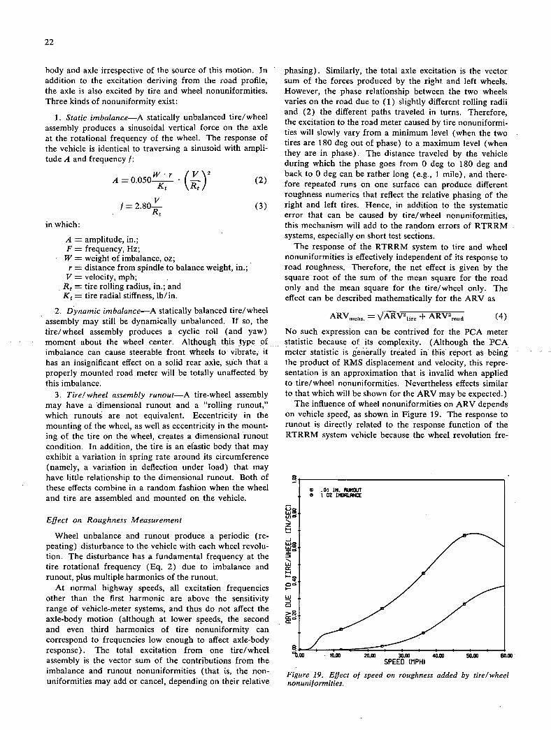
22

body and axle irrespective of the source of this motion. In addition to the excitation deriving from the road profile, the axle is also excited by tire and wheel nonuniformities. Three kinds of nonuniformity exist:

Static imbalance—A statically unbalanced tire/wheel assembly produces a sinusoidal vertical force on the axle at the rotational frequency of the wheel. The response of the vehicle is identical to traversing a sinusoid with ampli-tude A and frequency f:

A =0.O5Or . (±) (2)

(3)

in which:

A = amplitude, in.; F = frequency, Hz; W = weight of imbalance, oz;

r = distance from spindle to balance weight, in.; V = velocity, mph; Rt = tire rolling radius, in.; and K = tire radial stiffness, lb/in.

Dynamic imbalance—A statically balanced tire/wheel assembly may still be dynamically unbalanced. If so, the tire/wheel assembly produces a cyclic roll (and yaw) moment about the wheel center. Although this type of imbalance can cause steerable front wheels to vibrate, it has an insignificant effect on a solid rear axle, such that a properly mounted road meter will be totally unaffected by this imbalance.

Tire/wheel assembly runout—A tire-wheel assembly may have a dimensional runout and a "rolling runout," which runouts are not equivalent. Eccentricity in the mounting of the wheel, as well as eccentricity in the mount-ing of the tire on the wheel, creates a dimensional runout condition. In addition, the tire is an elastic body that may exhibit a variation in spring rate around its circumference (namely, a variation in deflection under load) that may have little relationship to the dimensional runout. Both of these effects combine in a random fashion when the wheel and tire are assembled and mounted on the vehicle.

Effect on Roughness Measurement

Wheel unbalance and runout produce a periodic (re-peating) disturbance to the vehicle with each wheel revolu-tion. The disturbance has a fundamental frequency at the tire rotational frequency (Eq. 2) due to imbalance and runout, plus multiple harmonics of the runout.

At normal highway speeds, all excitation frequencies other than the first harmonic are above the sensitivity range of vehicle-meter systems, and thus do not affect the axle-body motion (although at lower speeds, the second and even third harmonics of tire nonuniformity can correspond to frequencies low enough to affect axle-body response). The total excitation from one tire/wheel assembly is the vector sum of the contributions from the imbalance and runout nonuniformities (that is, the non-uniformities may add or cancel, depending on their relative

phasing). Similarly, the total axle excitation is the vector sum of the forces produced by the right and left wheels. However, the phase relationship between the two wheels varies on the road due to (1) slightly different rolling radii and (2) the different paths traveled in turns. Therefore, the excitation to the road meter caused by tire nonuniformi-ties will slowly vary from a minimum level (when the two tires are 180 deg out of phase) to a maximum level (when they are in phase). The distance traveled by the vehicle during which the phase goes from 0 deg to 180 deg and back to 0 deg can be rather long (e.g., 1 mile), and there-fore repeated runs on one surface can produce different roughness numerics that reflect the relative phasing of the right and left tires. Hence, in addition to the systematic error that can be caused by tire/wheel nonuniformities, this mechanism will add to the random errors of RTRRM systems, especially on short test sections.

The response of the RTRRM system to tire and wheel nonuniformities is effectively independent of its response to road roughness. Therefore, the net effect is given by the square root of the sum of the mean square for the road only and the mean square for the tire/wheel only. The effect can be described mathematically for the ARV as

ARVnieas = VARy2 tire road + ARV2 (4)

No such expression can be contrived for the PCA meter statistic because of its complexity. (Although the PCA meter statistic is generally treated in this report as being the product of RMS displacement and velocity, this repre-sentation is an approximation that is invalid when applied to tire/wheel nonuniformities. Nevertheless effects similar to that which will be shown for the ARV may be expected.)

The influence of wheel nonuniformities on ARV depends on vehicle speed, as shown in Figure 19. The response to runout is directly related to the response function of the RTRRM system vehicle because the wheel revolution fre-

8

.01 IN. RIIIWT e

10.8 20.03 30.8 40.8 50.8 60.8' SPEED (MPH)

Figure 19. Eftect of speed on roughness added by tire/wheel nonuniformities.

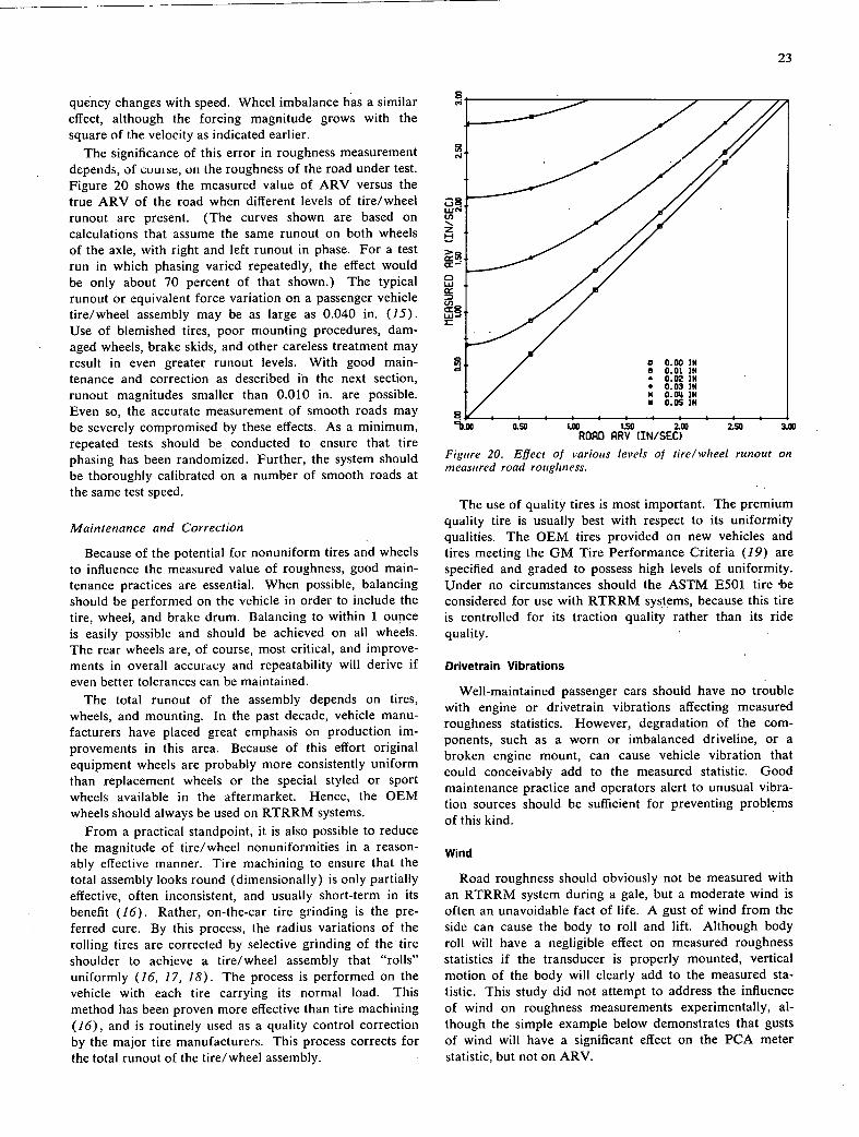
23

quency changes with speed. Wheel imbalance has a similar effect, although the forcing magnitude grows with the square of the velocity as indicated earlier.

The significance of this error in roughness measurement depends, of coutse, on the roughness of the road under test. Figure 20 shows the measured value of ARV versus the true ARV of the road when different levels of tire/wheel runout are present. (The curves shown are based on calculations that assume the same runout on both wheels of the axle, with right and left runout in phase. For a test run in which phasing varied repeatedly, the effect would be only about 70 percent of that shown.) The typical runout or equivalent force variation on a passenger vehicle tire/wheel assembly may be as large as 0.040 in. (15). Use of blemished tires, poor mounting procedures, dam-aged wheels, brake skids, and other careless treatment may result in even greater runout levels. With good main-tenance and correction as described in the next section, runout magnitudes smaller than 0.010 in. are possible. Even so, the accurate measurement of smooth roads may be severely compromised by these effects. As a minimum, repeated tests should be conducted to ensure that tire phasing has been randomized. Further, the system should be thoroughly calibrated on a number of smooth roads at the same test speed.

Maintenance and Correction

Because of the potential for nonuniform tires and wheels to influence the measured value of roughness, good main-tenance practices are essential. When possible, balancing should be performed on the vehicle in order to include the tire, wheel, and brake drum. Balancing to within 1 ounce is easily possible and should be achieved on all wheels. The rear wheels are, of course, most critical, and improve-ments in overall accuracy and repeatability will derive if even better tolerances can be maintained.

The total runout of the assembly depends on tires, wheels, and mounting. In the past decade, vehicle manu-facturers have placed great emphasis on production im-provements in this area. Because of this effort original equipment wheels are probably more consistently uniform than replacement wheels or the special styled or sport wheels available in the aftermarket. Hence, the OEM wheels should always be used on RTRRM systems.

From a practical standpoint, it is also possible to reduce the magnitude of tire/wheel nonuniformities in a reason-ably effective manner. Tire machining to ensure that the total assembly looks round (dimensionally) is only partially effective, often inconsistent, and usually short-term in its benefit (16). Rather, on-the-car tire grinding is the pre-ferred cure. By this process, the radius variations of the rolling tires are corrected by selective grinding of the tire shoulder to achieve a tire/wheel assembly that "rolls" uniformly (16, 17, 18). The process is performed on the vehicle with each tire carrying its normal load. This method has been proven more effective than tire machining (16), and is routinely used as a quality control correction by the major tire manufacturers. This process corrects for the total runout of the tire/wheel assembly.

Th.m 030 In 1.50 2.W 2.50 3.00 RORD RRV (IN/SEC)

Figure 20. E/Ject of various levels of tire/wheel runout on ,neasured road roughness.

The use of quality tires is most important. The premium quality tire is usually best with respect to its uniformity qualities. The OEM tires provided on new vehicles and tires meeting the GM Tire Performance Criteria (19) are specified and graded to possess high levels of uniformity. Under no circumstances should the ASTM E501 tire be considered for use with RTRRM systems, because this tire is controlled for its traction quality rather than its ride quality.

Drivetrain Vibrations

Well-maintained passenger cars should have no trouble with engine or drivetrain vibrations affecting measured roughness statistics. However, degradation of the com-ponents, such as a worn or imbalanced driveline, or a broken engine mount, can cause vehicle vibration that could conceivably add to the measured statistic. Good maintenance practice and operators alert to unusual vibra-tion sources should be sufficient for preventing problems of this kind.

Wind

Road roughness should obviously not be measured with an RTRRM system during a gale, but a moderate wind is often an unavoidable fact of life. A gust of wind from the side can cause the body to roll and lift. Although body roll will have a negligible effect on measured roughness statistics if the transducer is properly mounted, vertical motion of the body will clearly add to the measured sta-tistic. This study did not attempt to address the influence of wind on roughness measurements experimentally, al-though the simple example below demonstrates that gusts of wind will have a significant effect on the PCA meter statistic, but not on ARV.

24

Consider a gust of wind that lasts 20 sec, with the effect of raising the vehicle in., and then dropping it back. The effect on the ARV statistic is a simple increase of 1 in., divided by the time of the test. Over 1 mile, this is an error of 1 percent on a moderately rough road. The PCA meter statistic is affected in two ways: (1) six spurious counts are added to the registers (three up, three down); and (2) equilibrium position is shifted by 112 in. during the gust, or, for 1 mile at V = 50 mph, the average equilibrium position is shifted by 0.14 in. This latter effect would serve to increase the PCA meter statistic (on a moderately rough road) by nearly 40 percent.

EVALUATION OF CALIBRATION METHODS

With so many variables influencing the roughness mea-surements of RTRRM systems, accurate and frequent calibration is the only practical means of obtaining con-sistent performance from these devices. This section pre-sents the findings from the evaluation and development of appropriate calibration methods for RTRRM systems. Calibration of an instrument is normally performed by measuring an input with a known absolute numeric asso-ciated with it. But prior to this research, neither a "standard road," with an established roughness level, nor a method for assigning a standard roughness numeric to a measured profile was available. Accordingly, a standard roughness measurement was developed that is a rigorously defined property of the profile of a pavement, and has an accuracy limited only by the accuracy of the profile mea-surement. In addition, the "standard road" concept was pursued, with the result that an artificial surface that has an associated roughness value was designed and fabricated. Calibration methods using standard measurements of exist-ing pavements and using artificial surfaces were then devised and tested on in-use RTRRM systems from various agencies.

Because the definition of a standard roughness measure is the vital first step in developing calibration procedures, this section first addresses this need and discusses a sug-gested roughness standard. Next, the research findings on the reasons that RTRRM systems behave as they do are used to define the scope that a calibration procedure must cover. In this discussion, many calibration methods sug-gested in the past are seen to be inappropriate and the number of valid calibration approaches is vastly reduced. Finally, the development of two calibration methods is presented, along with the more significant findings of the testing of in-use systems applying these methods. For a detailed description of the two methods, the reader is referred to Appendix A.

Standard RTRRM System Measurement

The standard for RTRRM system calibration would ideally be the present serviceability rating developed with the AASHO Road Tests (2). However, that measure is obtained from the subjective evaluation of road roughness by a rating panel and is neither convenient to obtain nor amenable to precise determination. The use of such a

standard would factor a random error into the calibration process, reducing the precision with which it can be per-formed and reducing its effectiveness as a means of main-taining consistent performance from RTRRM systems. The slope variance as measured by the CHLOE is a second candidate with historical roots that merit its consideration. However, the CHLOE roughness measurement has been found to derive from a band of profile wave numbers much broader than is significant to an automotive vehicle and as a result introduces a random error that degrades the agree-ment between RTRRM system measurements and the CHLOE statistic. Correlations between PSI (derived from a simulated CHLOE) and ARV measurements from vari-ous RTRRM systems are presented in Appendix B, and generally show random errors between PSI and ARV that are twice as large as random errors between ARV measure-ments obtained from different RTRRM systems.

For maximum utility, the standard RTRRM system roughness statistic should be selected to best agree with measurements taken by the diverse population of RTRRM systems. Additionally, the measure of roughness should closely reflect the roughness features most critical to the public's judgment of the road.

Published data indicating the relative importance of roughness wave number on the ride acceptability of a roadway are sparse. A comprehensive subjective ride study was conducted by the Michigan Department of Transporta-tion with the purposeof identifying the relative importance of wave number on ride perception (11). In the study, 32 road surfaces were subjectively evaluated by 85 subjects in a variety of vehicles, answering the question, How is the road? The measured road profiles were then analyzed to determine a wave number weighting function that could be used to provide a weighted mean-square. elevation statistic that best correlates with subjective rating. The results indicated that the roughness contained in the wave numbers ranging between 0.02 and 0.5 cycle/ft (1.5 to 37 Hz at 50 mph) correlated the strongest with subjective rating. These data suggest that the higher frequency vibration that is associated with the axle resonance should be reflected in the roughness statistic in order to best agree with ride perception. Further, human sensitivity to vertical vibration is suspected to be maximum in the range of 5 to 6 Hz, decreasing at higher and lower frequencies. Figure 21 shows a typical acceleration spectrum measured on a passenger car by Smith (20) in a subjective ride study, along with ride comfort boundaries that have been adopted by the International Standard Organization (21). Typi-cally, vibrations in the region of the axle resonance fre-quency most closely and broadly encroach on the comfort boundary—a finding that supports the MDOT result. All in all, this type of evidence suggests that a relevant measure of road roughness must substantially reflect high frequency (high wave number) roughness content. Of the two popular RTRRM system roughness statistics in use, only the ARV (or I/M) statistic meets this requirement.

A reference RTRRM system measuring the ARV sta-tistic was therefore adopted as a calibration standard for this project, and is further recommended as a pavement serviceability standard in Chapters Three and Four.

b.00 4.00 8.00 12.00 16.00 20.00 24.00 FREQUENCY (HZ)

25

The reference system is defined in terms of its dynamic response characteristics, making it invariant with time, and a well-defined (although complicated) function of pave-ment profile. Its precision is limited only by the fidelity between the physical implementation of the system and its specifications. The essential components and response characteristics are shown in Figure 22. The system is linear and consists of a sprung and unsprung mass with suspension and tire springs and suspension damping. The average of the left and right wheel track profiles is the input, and the axle-body motion is the output. This HSRI reference system could be implemented in hardware but, as is the case with existing RTRRM systems, would present difficulties in achieving and maintaining the desired re-sponse characteristics. The vehicular components consti-tute the major problem, because the meter portion itself could be made as perfect and ideal as desired by use of electronic components (see App. B). In practice, the HSRI reference is most easily implemented as a system simulation linked to actual profile measurements, in which case the accuracy of a reference ARV (RARV) measure-ment is limited by the accuracy of the profile measurement. RARV is, in fact, a completely defined property of a pavement profile, and cannot actually be measured by a normal RTRRM system with different response properties. Rather, the RTRRM system produces measurements that correlate strongly enough with RARV statistics that they can be corrected to yield calibrated ARV (CARV) statis-tics that should agree well with the true RARV values.

This type of reference system is not new. In fact, it is similar to the quarter-car simulations of BPR roughometers or passenger cars, as used with profilometers in the past (8). However, the performance characteristics of the HSRI reference have been selected so as to minimize differences between RARV values and CARV mcasurc-ments taken with existing RTRRM systems. More im-portant, its quality as a reference for defining standard roughness values has been tested and found superior to all other proposed or existing systems, as is discussed later. Although it is true that RARV measurements will have some level of correlation with all of the other roughness statistics that are in use, different roughness statistics describe different qualities of pavement profile and are not deterministically related. Faced with a multitude of rough-ness statistics, the most straightforward and logical step towards promoting agreement between measurements made by different agencies is to adopt the best of the existing statistics, and abandon use of the rest for present and future work. At this time, the RARV appears to be the best statistic, although it is likely that future research will produce a better statistic that can then be adopted. Con-sequently, efforts were directed only towards calibrating RTRRM systems measuring ARV.

Conditions Required for Calibration

c'J9 I.

— I J

I b-i '

7b0 ' '''Ibi ' ' ' •

FREQUENCY (112) Figure 21. Comparison of measured spectral density of pas-senger acceleration with ISO vibration standards.

M5Z5 + C5(2545) + K5(Z5_Z) = 0

M525 + MZ + K t Z U = I(tL

Ks/Ms

Sprung Mass Kt/M5 653 1/sec2

= 62.3 1/sec2

115 U/Ms = .150

Dunper Suspension

C5/M5 = 6.00 1/sec

llll Cs Spring

92 K5

Acalibration is not valid unless it demonstrates the relationship of the system being calibrated to a standard AXLE-BODY RESPONSE FUNCTION OF NSA! REFERENCE SIMULATION over conditions encompassing the full intended measure- Figure 22. Dynamics of reference road roughness measurement ment range. system.

26

The earlier discussion of RTRRM system variables identifies the meters and rear suspension components as the elements directly influencing the measurement of road roughness. Hence their properties must be quantified in terms of ARV measurement during calibration. Prior to this research, there existed hope among RTRRM system users that there might be simple tests that adequately characterize the system response. For example, can re-sponse measures obtained on simple eccentric drum devices, or can separate tests of shock absorber damping, answer the need?

Response tests similar to that which would be performed with eccentric drum rollers or a simple hydraulic exciter were conducted at the TARADCOM facility. However, the understanding of RTRRM system function achieved over the course of this research has pointed out the diffi-culties of using these simple methods. First, vehicle re-sponse is nonlinear, depending on the frequency and amplitude of the roughness input, as was shown in Fig-ure 18. Hence, testing sufficient to characterize the vehicle response function must cover a range of amplitudes at a given frequency, with the appropriate amplitude range changing with frequency. At the axle-resonance frequency, amplitudes must be as small as 1A6 in. or less to be repre-sentative of real roads. Although the measurement of the vehicle response function will quickly identify any changes -in-the -vehicle--portion - ofanRTRRM system -(and, it is inevitable that changes will be observed), the effect on roughness measurement on-road is not easily obtained. (Tests at TARADCOM and measurements of separate vehicular component properties showed that response tests used together with a quarter-car model are not adequate for accurately predicting changes in on-road roughness measurements. As a minimum, a more complex vehicle model would be needed.) Secondly, road meter instru-ments, as presently limited by hysteresis and quantization effects, are inadequate for measuring vehicle response at the low amplitudes needed with sinusoidal excitation. Additional instrumentation in the nature of displacement transducers and recorders would be required.

Ultimately, it is the entire range of road roughness, acting simultaneously, that makes the systems function as they do. Hence, full spectrum roughness excitation is a necessary condition for calibration.

The most straightforward approach that guarantees full spectrum excitation to an RTRRM system is simply the use of real roads for calibration. Ideally, one rough road and one smooth road would be sufficient, but in practice such a small number is sure to bias the calibration. Even after the best calibration, different RTRRM systems tra-versing a road (that was not included in the calibration exercise) will yield a range of roughness measures for that road. This is because differences in the response character-istics of the RTRRM systems combine with peculiarities in the spectral content of the pavement to introduce a differ-ence between roughness measurements. The peculiarities are unique to each section of pavement; hence the resulting differences in measurement appear as random errors. To prevent this type of random error from biasing the calibra-tion—and later causing a systematic error when measure-

ments are corrected according to the calibration—the calibration should include a number of real roads. Given the existence of a random error after calibration, it is not cost effective to completely eliminate systematic errors; rather, they should be reduced to a level that is insignificant relative to the random error. For this purpose, about 10 roads of one construction type, spread over the roughness range of the calibration, appear to be adequate on the basis of the limited data acquired during the project.

If systems were to be used exclusively at 50 mph, calibra-tion at that speed only would be sufficient. However, they are frequently used at other speeds such that the contribu-tion of roughness from tire/wheel nonuniformities will vary, as will the perceived frequency content of the road excitation. Therefore, calibration should encompass not only a range of roughness conditions but also a range of speed conditions.

A second valid calibration approach is to excite the RTRRM system with full spectrum roughness from a source other than actual real roads. Here, the first question that must be addressed is, What spectrum should be used? While real roads have roughness properties that are char-acterized by unique spectral distributions, Appendix A shows that there is a commonality to roads that provides the basis for an "average road" concept (even though the "average bituminous road" differs slightly from the "aver-age- PCC road"), as discussed earlier in the section titled "Theory of Operation." In theory, calibration could be achieved with just several average roads because unknown errors resulting from peculiarities of actual individual roads would be eliminated.

Because RTRRM system measurements are increased by the response to tire/wheel nonuniformities, systematic errors can be introduced if the calibration excludes or distorts these effects by causing the wheels to rotate at a rate different from the rotational frequency during normal use (see Fig. 19). An example of this type of calibration is the use of hydraulic shakers to provide excitation, which calibration requires that the wheels not rotate at all. These errors have been shown to be more significant on smoother roads (see Fig. 20); hence such a calibration could be valid on medium and rough roads—but not on smooth roads.

Various Calibration Methods

Local Reference Surfaces

A series of local road surfaces is commonly in use today for running calibration checks of RTRRM systems. The method- is quite convenient, but involves an uncertainty because actual roads are constantly changing with time. For example, slab curl on PCC surfaces has been demon-strated to vary even over a one-day period (7). Ultimately, this method suffers, at present, from the inability to assign a precise standard value of roughness to the surfaces at any point in time, although an effective solution to this problem is to assign RARV values to the roads periodically with a profilometer/quarter-car simulation. On the basis of this solution, three slightly different applications of this method are described in Chapter Three.

27

Central Calibration Site

A series of surfaces at a central calibration site has been proposed. This scheme would parallel the Area Regional Reference Center approach to skid tester calibration. However, the surfaces would be substantially more expen-sive than surfaces with standardized skid numbers, and the logistical problems of going to the calibration center would preclude calibration as frequently as desired or needed. Altogether, this method does not appear to be cost effective in that the necessary funding would be better spent on obtaining profilometer calibration equipment.

Hydraulic Road Simulator

The hydraulic road simulator (or "shaker system") is potentially a precise means of subjecting an RTRRM sys-tem to specific road inputs which could be either a variety of real road profiles or several average road profiles. An adequate system, however, is potentially expensive ($30,000 to $50,000 just for the hardware) and requires trained operating personnel. Calibration could be obtained by comparing RTRRM system roughness measurements to the known roughness levels of recorded surfaces. However, the method is not foolproof in that, the dynamic stiffness and nonuniformity characteristics of rolling tires are not replicated. This method was not tested because the needed facilities were not available for day-to-day calibration. The high cost associated with a hydraulic shaker system forced the conclusion that cheaper methods, if developed, would be more acceptable to the highway community.

Drum Rollers

Drum rollers can be used to generate excitation at many frequencies with amplitudes selected to best represent road excitation, and include rolling tire effects. The lowest frequency component is determined by the rotational speed of the drum, with the opportunity for adding components of roadway roughness at each multiple of that frequency by choice of the actual surface profile of the drum. Of course, to replicate 50-mph operation with the necessary 1-Hz body resonance excitation, drums 70 ft in circum-ference (22 ft in diameter) would be required. On the other hand, to reduce the drum size while retaining the low frequency portion of the spectrum implies testing at lower speeds. Operations at low speed are limited, however, by the phenomenon of "tire envelopment" of high frequency roughness caused by the "swallowing" of small bumps within the tire contact patch. The practical limit on mini-mum test speed was found to be approximately 15 mph (App. A), thus requiring a drum at least 7 ft in diameter. At this low speed, effects of tire/wheel nonuniformities are distorted, but the most fundamental problem with this method is that the rotating drum provides a strictly periodic excitation, and the adequacy of this type of excitation for representing road excitation is unknown. The response of the vehicle will be overly sensitive to the relation between the body resonance frequency and the drum rotational frequency, and whether or not a procedure can be devised that reduces this sensitivity is uncertain. This method was

not pursued because its success was not guaranteed, and because 7-ft drums were not available for testing with real RTRRM systems. Note that earlier attempts ,involved only a single harmonic (e.g., Neal (22) tried an eccentric drum arrangement) and failed because they cannot be related to the full-spectrum excitation provided by roads.

Artificial Surfaces

Calibration can be achieved by adding a known profile (with a known RARV value) to an existing road surface. Conceptually, this method is similar to the drum roller method with the drum surface "unwrapped" and placed on a smooth surface. A drawback with this approach is that existing pavements are not as smooth as drums, but this method has the important advantage that the length of the surface need not be limited. This method also requires low calibration speeds, because the roughness of the underlying pavement then becomes less significant. Thus tire/wheel nonuniformities are not properly compensated by the calibration. Earlier attempts at calibrating RTRRM sys-tems by running the system over objects attached to a pavement (23, 24), such as pipes, rubber pads, etc., were inadequate because the bumps did not provide full spec-trum excitation representative of real roads. Even recog-nizing that a low-speed artificial surface calibration is not effective for roughness measurements of smooth' roads, its potential as a low-cost method of performing a calibration merited its examination in this study.

Evaluation of Two Calibration Methods

On the basis of the evaluation of different approaches to calibration considered, two methods of calibration were selected for testing in the project. Calibration by correla-tion of RTRRM system ARV measurements against simul-taneous RARV measurements on actual roads is the first method. The second method is calibration by traversing artificial bumps that have known absolute RARV rough-ness values. A test of these methods was obtained in the Correlation Program (see App. B). Both methods are developed in Appendix A, and the calibration procedures are described in the ASTM format for standard test meth-ods.

Calibration Against a Pro filometer

The basic process of calibrating against RARV measure-ments provided by a GMR profilometer with the HSRI reference simulation is straightforward and has already been described. The major development work consisted of selecting the ARV statistic as a standard and selecting the response properties of the reference simulation. Sub-sequent on-road testing served to provide data that quan-tifies the adequacy of these selections.

Eight RTRRM systems and the new West Virginia pro-filometer were brought to HSRI in order to conduct a Correlation Program. The West Virginia profilometer was a recent acquisition from K.J. Law Engineers, Inc. (Model 690D) and consisted of a conventional vehicle-mounted profilometer with two road-follower wheels used to sense

28

the road profile in the left and right wheel tracks. The system's performance is equivalent to that of earlier units, although data processing is handled in the digital rather than analog form. The digital system was programmed with the HSRI reference simulation defined earlier. Re-gardless of profilometer speed, the traversal speed of the quarter-car simulation was always set at that prescribed for RTRRM systems to produce the proper (speed de-pendent) RARV statistic for each of 24 road test sites. (The simulation, as implemented, actually produced the total cumulative axle-body displacement, which was later converted to the RARV statistic by dividing by time needed to traverse each section at the specific speed.)

The general agreement between the RTRRM test systems and the standard RARV measurements from the profilom-eter/quarter-car simulation is shown in Figure 23, which is a plot of the mean and spread of the ARV measurements of the eight RTRRM systems versus RARV. A well-defined relationship exists up through RARV levels of 2.75 in/sec. Above this level, the differences increase, and the RARV measurements tend to be higher than those of the actual RTRRM systems. The cause of this effect is uncertain. Bounce of the profilometer follower-wheel on these rougher surfaces was originally suspected as a cause, but later retests at lower speeds disproved this mechanism. The suspected reason is that the HSRI reference, as imple-mented, does not include tire-enveloping effects. For a variety of technical reasons, outlined in Appendix B, the data taken were not sufficient to determine whether or not tire enveloping caused the discrepancies shown in the figure.

Standard Deviation

Mean -

RARV (in/nec)

Figure 23. Comparison of measured ARV from eight uncali-brated RTRRM systems to the standard (24 surfaces).

Notwithstanding this limitation, these results are taken as an indication that the RARV statistics can be obtained validly with a profilometer! quarter-car simulation and then used as a basis for calibrating RTRRM systems. The validity is limited to the roughness range of 0 to 2.75-in.! sec RARV, with the further condition that the profilometer be operated at reduced speeds (this is reduced profilometer measurement speed, not reduced simulated HSRI reference speed) as necessary on the rougher surfaces to avoid follower-wheel bounce. The practical consequences of the limited roughness range are negligible in that the 2.75 in./sec RARV (equivalent to 200 in./mile at 50 mph) is at the reasonable limit of roughness acceptable to the motoring public for high-speed highways.

Differences between roughness measurements produced by an RTRRM system and the reference are due to both differences in the basic response functions and to peculiari-ties in the properties of individual sections of pavement. Those differences that are due solely to differences in the RTRRM system response properties are systematic and can hopefully be completely corrected by calibration. But the peculiarities of the individual pavements and RTRRM system response functions together result in differences that are effectively random and are not eliminated by calibra-tion. Differences between the standard RARV numerics and the corrected roughness numerics that are derived from RTRRM systems are, of course, the errors in the RTRRM system measurements, and the magnitude of these errors defines the precision of the RTRRM system. The magnitude of these random errors also serves to show the quality of the reference numeric. Although the total elimination of the random errors associated with RTRRM system measurement is impossible, given that no two RTRRM systems have identical response properties, the judicious selection of the reference can minimize these errors.

Each RTRRM system that participated in the Correla-tion Program was calibrated by linearly regressing the ARV measurements of the system with the corresponding RARV measurements. The regression line was then used to correct the ARV measurements, yielding CARV nu-merics. Figure 24 illustrates the accuracy of RTRRM systems calibrated in this fashion by showing the mean values and standard deviations of the calibrated measure-ments from the 8 systems versus RARV for the 18 surfaces. Comparing this plot to Figure 23 shows the improvement obtained from the calibration. Figure 24 reveals an important point about the errors obtained even after calibration—namely, that the errors tend to be con-sistent in magnitude over the entire roughness range. As a result, they tend to be percentage-wise much more signifi-cant on smoother roads.

In analyzing the results to determine the adequacy of the HSRI reference, each of the RTRRM systems was treated as a candidate reference, thus defining calibration by the linear regression correlation of the candidate refer-ence with each other system. The average random error using the HSRI reference was near the lowest of those produced, indicating that the HSRI reference is a good choice for an RTRRM reference. This finding is also

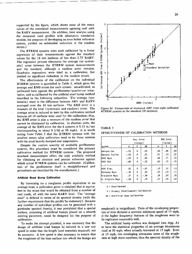
29

supported by the figure, which shows most of the mean values of the correlated measurements agreeing well with the RARV measurement. (In addition, later analysis using the measured road profiles with alternative simulation models, for purposes of developing an even better reference system, yielded no substantial reduction in the random errors.)

The RTRRM systems were each calibrated by a linear regression of their measurements against the standard values for the 18 test surfaces of less than 2.75 RARV. The regression process eliminates the average (or system-atic) error between the RTRRM system measurements and the standard, although a random error remains. Quadratic regressions were tried as a calibration, but yielded no significant reduction in the random errors.

The effectiveness of the calibration on the individual RTRRM systems is quantified in Table 5, which gives the average and RMS errors for each system: uncalibrated, as calibrated here against the profilo meter/ qu arter-car simu-lation, and as calibrated by the artificial road bump method described in the following subsection. The average (sys-tematic) error is the difference between ARV and RARV averaged over the 18 test surfaces. The RMS error is a measure of the total (systematic and random) error. The average error is reduced to zero by this calibration method because all 18 surfaces were used for the calibration; thus. the RMS error is also a measure of the random error that cannot be eliminated by calibration. In absolute units, the average of the RMS error for the 8 systems is 0.12 in./sec (corresponding to about 9 I/M at 50 mph). It is worth noting from Table 5 that the RTRRM systems with the smallest errors after calibration tend to be those systems with the most heavily damped rear suspensions.

Despite the current scarcity of available profilometer systems, this procedure must be considered the primary calibration method for RTRRM systems. The proposed standard measurement offers the only available method for obtaining an absolute and precise reference against which actual RTRRM systems can be calibrated. (Calibra-tion of the profilometer itself is straightforward and procedures are described by the manufacturer.)

Artificial Road Bump Calibration

By traversing on a roughness profile equivalent to an average road, a calibration point is obtained that is equiva-lent to the mean that would be obtained from a number of real roads, all with the same RARV level. The "average road" is defined in terms of its spectral density (with the further requirement that the profile be stationary). Because any number of individual profiles can be generated with a particular spectral density, it was postulated that a special surface, consisting of artificial bumps placed on a smooth existing pavement, could be designed for the purpose of calibration.

To make the attempt practical, it was necessary that the design of artificial road bumps be tailored to a low test speed in order that the length (and materials required) not be excessive. A low speed is also necessary to ensure that the roughness of the base surface (on which the bumps are

Mean

Standard Deviation

0 1

RARV (in/sec)

Figure 24. Comparison of measured ARV from eight calibrated RTRRM systems to the standard (18 surfaces).

TABLE 5

EFFECTIVENESS OF CALIBRATION METHODS

Ave. Error RMS Error

(in/sec) (in/sec)

U P AD U P I AD

Georgia Car -.25 0 .25 .26 .09 .29

Georgia Trailer -.50 0 .23 .51 .10 .27

HSRI Mays -.24 0 .04 .26 .11 .12

HSRI PCA -.60 0 -.02 .63 .15 .15

HSRI Elec. .02 0 -.01 .12 .12 .13

Kentucky Mays -.26 0 .05 .27 .10 .11

Wisconsin Mays .21 0 -.06 .24 .12 .15

W. Virginia Mays -.06 0 .14 .21 .15 .22

ii = Uncalibrated

P = Primary (Profilometer) Calibration

AD = Artificial Bump Calibration

emplaced) is insignificant. Tests of the enveloping proper-ties of tires dictated a nominal minimum speed of 15 mph, if the higher frequency features of the roughness wereto be replicated reasonably well.

The artificial bump surface was designed (see App. A) to have the statistical properties of an average bituminous road at 50 mph, when actually traversed at 15 mph. Even at 15 mph, tire enveloping attenuates some of the rough-ness at high wave numbers; thus the spectral density of. the

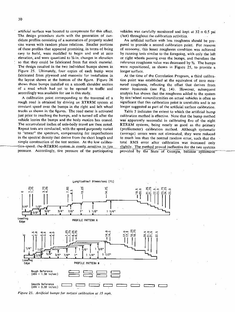
30

artificial surface was boosted to compensate for this effect. The design procedure starts with the generation of can-didate profiles consisting of a summation of properly scaled sine waves with random phase relations. Smaller portions of these profiles that appeared promising, in terms of being easy to build, were modified to begin and end at zero elevation, and were quantized to 1/8-in. changes in elevation so that they could be fabricated from flat stock material. The design resulted in the two individual bumps shown in Figure 25. Ultimately, four copies of each bump were fabricated from plywood and masonite for installation in the layout shown at the bottom of the figure. Figure 26 shows these bumps installed on a smooth shoulder section of a road which had yet to be opened to traffic and accordingly was available for use in this study.

A calibration point corresponding to the traversal of a rough road is obtained by driving an RTRRM system at constant speed over the bumps in the right and left wheel tracks as shown in the figures. The road meter is activated just prior to reaching the bumps, and is turned off after the vehicle leaves the bumps and the body motion has ceased. The accumulated inches of axle-body travel are then noted. Repeat tests are conducted, with the speed purposely varied to "smear" the spectrum, compensating -for imperfections in the spectral density that derive from the short length and simple construction of the test section. At the low calibra-

pressure. Accordingly, tire pressure of the participating

vehicles was carefully monitored and kept at 32 ± 0.5 psi (hot) throughout the calibration activities.

An artificial surface with less roughness should be pre-pared to provide a second calibration point. For reasons of economy, this lesser roughness condition was achieved by running tests similar to the foregoing, with only the left or right wheels passing over the bumps, and therefore the reference roughness value was decreased by . The bumps were repositioned, as shown in Figure 25, to provide a longer surface.

At the time of the Correlation Program, a third calibra-tion point was established at the equivalent of zero mea-sured roughness, reflecting the offset that derives from meter hysteresis (see Fig. 14). However, subsequent analysis has shown that the roughness added to the system by tire/wheel nonuniformities on actual vehicles is often so significant that this calibration point is unreliable and is no longer suggested as part of the artificial surface calibration.

Table 5 indicates the extent to which the artificial bump calibration method is effective. Note that the bump method was apparently successful in calibrating five of the eight RTRRM systems, being nearly as good as the primary (profilometer) calibration method. Although systematic (average) errors were not eliminated, they were reduced to much less than the normal random error, such that the total RMS error after calibration was increased only 1ightly. The method proved ineffective for the two systems provided by the

Longitudinal Dimensions.(ft)

In UI In 10 fl UI In In (fl C.J N. N. NI C) NJ CU Ul C) NJ I- UI C) N. NJ C) • . In . .

o .- r p.. . 0 010

1/4"

H ii

1

1/2

I jr

I I I 5/0 3/4" 7/0' 1" 1 1/0" 1 1/4"

LeadingEdge

PROFILE PATTERU A

100 010 UIO 001 (UP.. UI0UI UI

P-CU fifi NIp.- OC) 0-.- p.

'2'

71 1 1 11/2

Leadhg Edge PROFILE PATTERN B

Rough Reference F_1 ci L_ (ARV = 1.98 in/sec)

I I_111

Smooth Reference (ARV = 0.99 in/sec)

Figure 25. Artificial bumps for surface calibration at 15 mph.

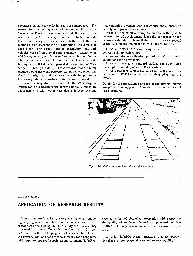
31

(average) errors near 0.25 in./sec were introduced. The reasons for this finding were not determined because the Correlation Program was conducted at the end of the research project. However, these two vehicles, as cali-brated, had nearly identical errors with the result that the method did an excellent job of "calibrating" the vehicles to each other. This result leads to speculation that both vehicles were affected by the same unknown phenomenon which may, or may not, be related to the calibration design. The method is also seen to have been ineffective in cali-brating the RTRRM system provided by the State of West Virginia. During the design, it was realized that the bump method would not work perfectly for all vehicle types, and the final design was tailored towards vehicles possessing heavy-duty shock absorbers. Simulations showed that errors of the magnitude introduced to the West Virginia system can be expected when lightly damped vehicles are calibrated with this method (see details in App. A) and

that equipping a vehicle with heavy-duty shock absorbers is likely to improve the calibration.,

All in all, the artificial bump calibration method, at its current state of development, lacks the confidence of the primary calibration. Nevertheless, it can serve several useful roles in the maintenance of RTRRM systems:

As a method for monitoring system performance between primary calibrations.

As an interim calibration procedure before primary calibrations can be available.

As a time-stable, standard surface for quantifying the long-term stability of an RTRRM system.

As a standard surface for investigating the sensitivity of individual RTRRM systems to variables other than tire effects.

Details for the construction and use of the artificial bumps are provided in Appendix A in the format of an ASTM test procedure.

/••• .1•' \••

Figure 26. Calibration surface with artificial bumps.

CHAPTER THREE

APPLICATION OF RESEARCH RESULTS

Given that roads exist to serve the traveling public, highway agencies have been increasingly' concerned in recent years about being able to quantify the serviceability of a road to its users. Generally, the ride quality of a road is foremost in the public judgment of serviceability. Hence the primary goal of agencies who measure road roughness with response-type road roughness measurement (RTRRM)

systems is that of obtaining information with respect to the quality of roadways defined as "pavement service-ability." This objective is impacted by concerns in many areas:

1. Which RTRRM systems measure roughness proper-ties that are most reasonably related to serviceability?

32

How do the RTRRM and dissimilar systems compare (correlate) in roughness measurements?

What calibration methods can be used for RTRRM systems, and what accuracy may be expected?

What are the appropriate applications and limitations of currently available RTRRM systems?

What improvements in roughness measurement can be implemented immmediately, and what future develop-ments can be anticipated?

This chapter summarizes the findings and suggestions (deriving from the research performed in this study) that provide answers to the previously posed questions.

PAVEMENT SERVICEABILITY

Roadway roughness spans a broad range of wave num-bers (wave number= 1/wavelength), but only a small portion affects the ride experienced by a user of the road in his/her vehicle. This portion is a function of the dy-namic properties and speed of the vehicle and the frequency sensitivity of human subjects to vibration. Ideally, a road roughness measuring system responds to the same portion of the total roughness and with the same weighting that determines a typical "ride." As seen in Figure 21, vehicle vibration on-road is broad band. The low frequency vibra-tions experienced from 0 to 20 Hz are caused primarily by the uneven road profile. Above this frequency range, the vibrations tend to be caused by excitations other than what is created by the macroscopic profile of the road—for example, the engine, the drive train, etc. RTRRM systems, being based on passenger vehicles, accordingly respond to that portion of the roughness spectrum to which passenger car occupants are exposed. The actual range and weighting of the roughness, though influenced by vehicle response, is dominantly established by the choice of measured statistic. Developing a system that would be exactly equivalent to the total ride process wherein a judgment is made is well beyond the current understanding of human response to vibration, and thus was not an objective of this research. However, the measurement performance of existing RTRRM systems was examined in the light of what is known about ride judgment in order to achieve better correlation to pavement serviceability.

The findings from the study have established that two basically different statistics are measured by RTRRM systems. The Mays meter measure is used to yield an approximation of inches/mile (I/M) where the "inches" refer to total accumulated axle motion relative to the car body. The PCA meter measures a unique statistic with units inches2/mile, which is amplitude weighted. No deterministic relationship exists between these statistics or with most of the many other roughness measurements now in use. Statistical correlations exist between them because of the correlation between the various portions of the overall road roughness measured by each type of system. In other words, high roughness content in one wave number range tends to be accompanied by high roughness content in another wave number range. (This relationship is, however, only a trend and is not consistently the case.) Whereas RTRRM systems are sensitive only to the wave

number range that affects the vehicles of the using public, the CHLOE measures over a much broader range. On the other hand, the range of the low speed BPR roughometer is offset to higher wave numbers because it operates below normal traffic speeds.

Given the multitude of roughness statistics now in use to estimate pavement serviceability, and given the lack of perfect agreement between them, the most practical first step towards meeting the goals of this program is the selection of the best measure for use by everyone and the abandonment of the rest. The recommended measure should be the one that best reflects pavement serviceability, but, at the same time, can be adopted by agencies using other measures, with a minimum of effort.

Recommended Roughness Statistic

The statistic measured by the Mays meter is derived from a relatively uniform weighting of frequencies in the range of 0 to 20 Hz, as shaped by the response of the vehicle. The PCA meter statistic is dominantly a measure of low frequency (0 to 2 Hz) response to road roughness. Of the two statistics, the I/M type of statistic is the more rational choice as a measure of road roughness closely related to serviceability because it includes the higher frequencies known to influence the judgment and reaction of the road. user. Fortuitously, it also appears less sensitive to vehicle variables. Further, this statistic can also be measured by a PCA meter by simplifying the manner in which the roughness data is summed (as described under "Theory of Operation" in Chapter Two and also in App. C).

The I/M statistic derives from early efforts to describe road roughness by summing the vertical deviations per unit of length. With the adoption of RTRRM systems, the more appropriate statistic is average rectified velocity (ARV) of the axle-body motion, which statistic is a com-parable measure of inches (of the axle-body motion) per unit time rather than per unit distance. The ARV divided by test speed, with appropriate unit conversion factors, is equal to I/M. The ARV statistic, as produced by RTRRM systems, is a preferred statistic for a number of reasons. First, ARV is a direct measure of the amplitude of vehicle response and is hence related to ride. Another advantage is that ARV measurements made at different speeds are comparable, unlike I/M measurements taken at different speeds. (A lower ARV measurement always indicates better ride, while I/M is both a function of ride and the time needed to travel 1 mile at the measuring speed.) Vehicle motion response is time- not distance-based. Scal-ing the vehicle response for calibration must be accom-plished at the level of ARV rather than I/M.

It is recommended that the PCA meter statistic be abandoned because of its sensitivity to variations in vehicle properties, the absence of sensitivity to high-frequency road roughness, its nonlinear properties, and its obscure rela-tionship to other recognized statistics. Commercial PCA meters can be used to measure ARV, usually with less effort than needed for the PCA meter statistic. Hence, old PCA meter data can be converted to yield ARV numerics to

33

provide Continuous records, through the years, of pavement roughness levels for particular roads. In the event that the old raw data—the counts in the individual regislers—are not available, the old PCA meter statistics would need to be converted to ARV via an empirical regression equation that would be determined by the agency for its particular RTRRM system, covering its normal range of operation.

Relationship to Serviceability

The current measure of pavement serviceability is a present serviceability rating (PSR) obtained by a method-ology developed by AASHO in the 1950's, which method requires a panel of highway users to individually assign PSR values to a specific road section. The relative error (taken as standard deviation of panel ratings, divided by mean panel rating) in the PSR statistics generated in the AASHO road tests averaged 19 percent, indicating that PSR has basic limitations in its precision.

In the AASHO program, the PSR figures were found to correlate well, but not perfectly, with the slope variance measured by AASHO profilometer (similar to the CHLOE profilometer) and, to a lesser extent, with other physical characteristics of the roads. These correlations were used to define a present serviceability index (PSI) based mainly on the CHLOE measurement, which can be used to esti-mate the PSR with a relative error of 15 poroont. Thco-retically, RTRRM systems can (now) be correlated with the CHLOE slope variance and related to PSI and PSR through the correlation curves developed by AASHO. But the separate correlations are sufficiently imperfect that the degree of correlation between an RTRRM system measure-ment and PSI involves significant uncertainty.

Figure 27 shows the PSI values determined for 18 road sections by (1) two of the state agencies participating in the Correlation Program who converted their RTRRM statistics to PSI and (2) a conversion of CHLOE slope variance to PSI by the AASHO formula where slope vari-ance was obtained from a simulation of the CHLOE profilometer traversing the profiles measured by the West Virginia profilometer. The resultant index was plotted as a function of the reference ARV (RARV) yielded by the reference RTRRM system suggested as a calibration standard. The scatter between PSI and RARV evident here is much greater than the scatter between calibrated (CARV) measurements made with different RTRRM systems (see App. B).

Notwithstanding this scatter, Figure 27 also shows a more or less linear trend between PSI and RARV, a finding that suggests that RARV is more or less a linear function of serviceability and therefore a reasonable statis-tic to be used until a better measure is developed. It should be noted that studies of ride perception (20) have indicated a linear relationship between subjective ratings and RMS acceleration over the normal range of vehicle vibration amplitudes. Hence a linear relationship between PSI and RARV would be expected.

The reduction of roughness measurements to corrected statistics by the means of the calibration procedures de-veloped in this project will provide a common basis for

. • U. U U U o • S 0

S

. S

000

d 0

U U

0 - based on CHLOE SV

- based on Kentucky meas.

- based on Wisconsin meas.

I I I

1.0 2.0 3.0

RARV (in/sec)

Figure 27. Comparison between PSI and ARV for three sources of PSI.

communication amongst the various practitioners. The perfect road (i.e., PSI = 5) is clearly equivalent to an RARV of zero. Figure 27 suggests that a marginal road (e.g., a PSI of 2.0) will yield an RARV of about 2.4 (170 I/M at 50 mph). Although an exact relationship between PSI and RARV cannot be defined on the basis of the data available at this time, it is expected that a common measurement language and a common calibration proce-dure will yield a better relationship, as user experience accrues. The practice of road roughness measurement, however, need not suffer in the meantime, because the RARV statistic appears to be adequate for ranking roads with respect to their roughness level and no significant advantage is gained from the additional conversion to PSI except as a link to past data.

CORRELATIONS

RTRRM Systems Measuring ARV

The agreement between individual instruments measur-ing the same physical parameter is never perfect, because the instruments can never be fabricated exactly to a given specification; but, ideally, it should be good enough such that random errors do not degrade the precision needed by the user. Measurement errors associated with RTRRM systems measuring the ARV statistic are currently high because of the individuality of the systems. Errors of 0.10 in./sec (approximately 10 percent of the RARV magnitude of a moderately rough road) appear to be the minimum that can be expected after calibrating typical systems now in use. (Correlations performed between

34

systems measuring dissimilar statistics are worse.) These errors derive from the individual nature of roads and of RTRRM systems and are, in essence, the random errors that remain after systematic errors have been, hopefully, removed by a calibration process involving a standard reference. It is unlikely that two RTRRM systems will yield comparable results if changes in operating conditions (tire pressure, air temperature, etc.) are not accounted for by frequent calibration.

The agreement between two RTRRM systems could be improved if the vehicle response characteristics and meter nonlinearities possessed by both systems are made similar. However, the response characteristics of vehicles are affected by so many operating variables that the efforts required to change the dynamic behavior of one vehicle to match that of another are far beyond the practical capabili-ties of the agencies that use RTRRM systems. In this particular context, shock absorbers constitute the most important elements affecting vericle response. Both experi-ments and calibrations have shown the agreement between any two RTRRM systems is improved when stiffer, heavy-duty shock absorbers are installed on vehicles. Further, the systems become less sensitive to unavoidable changes in operating conditions (e.g., tire pressure). Nevertheless, operators of RTRRM systems are sometimes reluctant to use stiff shock absorbers because the sensitivity of the system to road roughness is lowered, Overall, the research findings show that installation of soft shock absorbers increases errors in measurement of road roughness and should be discouraged.

A second important cause of poor agreement between RTRRM systems is meter hysteresis. Hysteresis results in a reduction of the measured roughness statistic, the extent of which is mainly sensitive to low frequency bouncing of the vehicle, which accounts for little of the total ARV measurement. Elimination of meter hysteresis should improve the correlation between different systems, namely, reducing the percent relative error from 10 percent to 5 percent (on a moderately rough road). The causes and amounts of meter hysteresis are generally specific to par-ticular instrument models. Consequently, agencies should examine their existing meters and, in consultation with the manufacturers, consider altering the meter to reduce hysteresis. When purchasing new meters, hysteresis levels should be specified and included in the criteria for selecting one instrument over another.

It is recommended that agencies abandon any efforts to correlate roughness measurements made at different speeds. Rather, measurements should always be made at a speed representative of normal mean traffic speeds, because it is the ride obtained by the users at normal traffic speeds that determines the serviceability of the pavement. Because ARV, and ride, change with speed, the measurement speed should be noted as part of the roughness numeric, perhaps as a subscript. Measurements that are made with the old BPR roughometer (at 20 mph) or with other RTRRM systems at reduced speeds should not be expected to corre-late well with RTRRM system measurements made at higher speeds, because different portions of the overall roughness spectrum are exciting the system.

Different Systems

The correlation between the ARV statistic and the CHLOE slope variance is of special interest because of the historical role of the CHLOE in the development of road roughness measuring systems and also because CHLOE slope variance is a direct measure of road profile. Ideally, the relationship between ARV and CHLOE is quadratic. (See "Theory of Operation" in Chap. Two and App. C for ideal relations between dissimilar systems.) Because less than 50 percent of the roughness measured by the CHLOE is measured by an RTRRM system, the relative error yielded by a correlation of these devices will generally be no better than 20 percent.

The correlation between ARV and the ideal PCA meter statistic should also be quadratic. In practice, the PCA meter statistic is also influenced by meter nonlinearities and is, itself, such a complicated nonlinear function of road roughness that the exact correlation relationship is un-known.

CALIBRATION

The calibration of an RTRRM system has not been a straightforward undertaking in that there are no surfaces of standard roughness that can be used to excite the system to check its measurement error. At best the RTRRM system can be exposed to a road with a known profile and its output compared to a well-defined statistical property of the profile. In correlating the output of RTRRM systems with a reference roughness numeric, systematic errors can be eliminated such that (over a broad range of roads) roughness numerics obtained by a calibrated RTRRM system will be neither high nor low on the aver-age. On the other hand, calibration cannot eliminate the random errors between a given RTRRM system and the reference statistic. Note that a major obstacle to achieving a precise calibration of RTRRM systems has been the ambiguous relationship between roughness statistics and the available standards (PSR, CHLOE slope variance, etc.). A significant result of this research has been the develop-ment of a standard of roughness defined in terms of a reference RTRRM system and the statistic to be measured. Additionally, a standard road for calibration of RTRRM systems was also developed to meet the needs of agencies with no immediate access to a profilometer who neverthe-less wish to calibrate their systems to a standard.

Good calibration practice serves two ends. First, users of RTRRM systems can compare measurements made by different agencies with different systems. For example, roads -in Georgia can be compared to roads in California. Second, and just as important, users of RTRRM systems can determine the sensitivities of their system to air tem-perature and other operating variables. Further, they can refine the general methodologies described in this report to suit their own requirements. Routine calibration activi-ties will enable system operators to improve their main-tenance practices and develop a full appreciation of the accuracy obtainable with such systems.

Reference System

A reference RTRRM system for calibration should

35

produce measurements that best reflect serviceability and, at the same time, correlate as well as possible with existing systems to reduce random errors. Insufficient data exist from which to optimize the reference system in its rela-tionship to serviceability, although a basis for the choice of the measurement statistic was developed, with the reference being selected so as to minimize the random errors.

The reference system is a linear quarter-car model of a representative passenger car. This model, defined by four parameter values, simulates the axle-body motion caused by the traversal of a road to yield the ARV statistic. The frequency response of the reference vehicle/simulation (the so-called HSRI reference) is typical of passenger cars equipped with heavy-duty shock absorbers. Because the response characteristics of the model are exact, the RARV is a completely deterministic function of the average pavement profile of the right- and left-hand wheel tracks, and its precision is limited only by the precision of the profile measurement.

An analysis of the data obtained in the Correlation Program, which included three profilometers and eight RTRRM systems, demonstrated (see App. B) that the HSRI reference is a better choice than the CHLOE slope variance or the old 1969 Impala quarter-car simulation, and provided measurements that correlated very well with measurements from the participating RTRRM systems. In the end, the correlation between RARV and ARV measurements from the other systems was generally better than the correlation between any two of the RTRRM systems.

The RARV of a surface can be calculated only if its profile is known. Although ARV measurements taken with RTRRM systems can be corrected after a calibration to agree better with the RARV values, they are not as precise. Hence, corrected ARV measurements are desig-nated as CARV.

Calibration Methods

Calibration with a Profilometer

The calibration method found to work best is the correla-tion (via linear regression) against a profilometer with the HSRI reference. The roads should include all levels of roughness and types of construction that will be rated with an RTRRM system. A separate calibration may be needed for roads of different construction and for different mea-surement speed, because the RTRRM system vehicle will respond differently to each. The calibration curve obtained generally does not pass through zero because of excess measured roughness deriving from tire/wheel nonuniformi-ties and/or losses in the measured statistic caused by hysteresis.

This calibration method is not new, but, as developed here, is the most effective method currently available. For this reason, it is referred to as the "primary" calibration. Clearly, the primary calibration should be used routinely by an agency that has a profilometer available. In agencies where a profilometer is not always available, other proce-dures may be used. Possible procedures and error sources are considered in the following and compared to the pri-

mary calibration in Table 6. Over the long term, a profile measurement capability must be acquired by agencies seriously intending to measure road roughness on a scale that is universally meaningful.

Secondary Vehicle Calibration

The simplest form of secondary calibration that could be used as an interim would involve the occasional calibra-tion of one RTRRM system and using it as a reference for other RTRRM systems, in more frequent calibrations. Any agency using this practice should be aware of two short-comings. (1) Measurement errors will be increased by 40 percent because of additional random errors. (Assum-ing the measurement errors from each system are inde-pendent, the expected RMS error is the orthogonal vector sum of the two errors. And if they are equal in magnitude,

this amounts to an increase by the ratio of V2, i.e., 40 percent.) (2) Undetected changes in the secondary refer-ence system will cause systematic errors in the calibration of other systems.

Calibration with Local Roads

Two calibration procedures that do not require continual access to a profilometer and use local roads may be con-sidered. The first procedure, local road calibration, re-quires selecting a test route involving local roads with various levels of roughness, and then conducting a primary calibration using a profilometer and reference system simulator. The roughuess numeric for each road is re-corded, and these figures are used for subsequent secondary calibrations without the profilometer. This method appears to be best for agencies that have limited access to a pro-filometer. Periodically, the profilometer must be brought back to check the roads for long-term changes. Clearly, the success of this procedure depends on the stability of the selected surfaces. At the time of their selection, the surfaces should be monitored extensively with a profilome-ter to identify the magnitude of variability resulting from daily and seasonal temperature changes, tailoring the selec-tion to minimize these errors.

The next procedure uses "average roads" as a means of minimizing the calibration time, but it requires occasional access to both a profilometer and a computer with spectral analysis software. The use of an arbitrary selection of local roads requires a fair number of roads in order to average out the unique peculiarities of each roadway, which peculiarities could bias the calibration. Two or three road sections could be used for calibration purposes, if it can be determined that these two sections have "average" properties; namely, they meet the following three condi-tions:

They cover the roughness range of interest to the user (as a minimum, one rough road and one fairly good road).

They have spectral densities that are close to the "average," within the range of wave numbers that influence the roughness statistic generated by an RTRRM system.

3 They are both statistically stationary, such that the

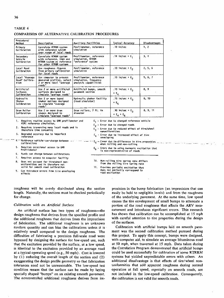
36

TABLE 6

COMPARISON OF ALTERNATIVE CALIBRATION PROCEDURES

Procedure/ Method Description Auxiliary Facilities jpjçal Accuracy Disadvantages

Primary Correlate RTRRM system Profilometer, reference .10 in/sec 1, 2 Calibration with reference system simulation

over range of local roads

Secondary Correlate RTRRM system Profilometer, reference .14 in/sec + E1 3, 4 Vehicle with reference, then use simulation, RTRRM Calibration RTRRM system as reference reference system

for other RTRRM systems

Local Road Use roughness figures Profilometer, reference .10 in/sec + E2 2, 5, 6 Calibration from primary calibration simulation

for local roads

Local Average Use computer to process Profilometer, reference .10 in/sec + E2 5, 6, 7 Road Calibra- omasured profiles, select simulation, frequency tion 2 or more local average analysis capabilities

roads

Artificial Use 2 or more artificial Artificial bumps, smooth .10 in/sec + E3 8, 9 Surfaces surfaces designed to pavement section + E Calibration simulate average roads' 4

Hydraulic Use 2 or more taped Hydraulic shaker facility .10 in/sec + C3 8, 10 Shaker shaker motions designed (road simulator) + E Calibration to simulate average 5 _______________ roads

Drum Roller Use 2 or more drum Drum rollers, 7 ft. in .1D in/sec + E3 8, 9, 11 Calibration shapes designed to diameter + E +

simulate 'average roads 4 6

Requires routine access to GMR profilometer and HSRI reference simulation.

Requires traversing many local roads and is therefore time consuming

Degraded accuracy due to imperfect reference

4Rêierhhce - - calibrations

Requires occasional access to GMR Profilometer

Roads can change between calibrations

Requires access to computer facility

Does not account for tire/wheel non-uniformities and is therefore not valid for smooth road calibration

Can introduce errors from tire enveloping effects

E1 - Error due to changed reference vehicle

- Error due to changed roads

E3 - Error due to reduced effect of tire/wheel nonuniformities

C4 - Error due to increased effect of tire enveloping

-E-Error-duc=to=difference in- tire-properties - - when rolling and non-rolling

E6 - Erors due to using harmonic excitation that is non-representative of roads

Non-rolling tire spring rate differs from the rolling tire spring rate

Provides periodic excitation that does not perfectly correspond to road excitation

roughness will be evenly distributed along the section length. Naturally, the sections must be checked periodically for change. -

Calibration with an Artificial Surface

An artificial surface has two types of roughness—the design roughness that derives from the specified profile and the additional roughness that derives from the imprecision of fabrication. The additional roughness is an unknown random quantity and can bias the calibrations unless it is relatively small compared to the design roughness. The difficulties of fabricating a precision fullscale road were bypassed by designing the surface for low-speed use, such that the excitation provided by the surface, at a low speed, is identical to the excitation provided by an average road at a typical operating speed (e.g., 50 mph). Cost is lowered by (1) reducing the overall length of the section and (2) exaggerating the design profile geometry so that fabrication tolerances need not be unreasonable. The low-speed test condition means that the surface can be made by laying specially shaped "bumps" on an existing smooth pavement. The noncontrolled additional roughness derives from im-

precision in the bump fabrication (an imprecision that can easily be held to negligible levels) and from the roughness of the underlying pavement. At the same time, low speed causes the tire envelopment of small bumps to attenuate a portion of the road roughness that affects the ARV mea-surement and introduces significant errors. This research has shown that calibration can be accomplished at 15 mph with careful attention to tire properties during the design of the surfaces.

Calibration with artificial bumps laid on smooth pave-ment was the second calibration method pursued during this project. To apply this concept, bumps were designed, with computer aid, to simulate an average bituminous road at 50 mph, when traversed at 15 mph. Data taken during the Correlation Program demonstrated that artificial bumps could be used successfully for calibration of some RTRRM systems but yielded unpredictable errors with others. An additional disadvantage is that effects of tire/wheel non-uniformities that add apparent roughness during normal operation at full speed, especially on smooth roads, are not included in the low-speed calibration. Consequently, the calibration is not valid for smooth roads.

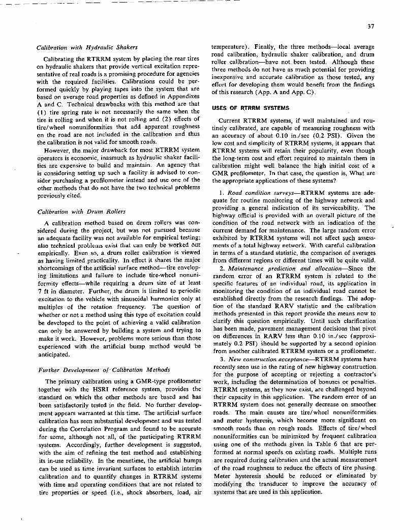
37

Calibration with Hydraulic Shakers

Calibrating the RTRRM system by placing the rear tires on hydraulic shakers that provide vertical excitation repre-sentative of real roads is a promising procedure for agencies with the required facilities. Calibrations could be per-formed quickly by playing tapes into the system that are based on average road properties as defined in Appendixes A and C. Technical drawbacks with this method are that (1) tire spring rate is not necessarily the same when the tire is rolling and when it is not rolling and (2) effects of tire/wheel nonuniformities that add apparent roughness on the road are not included in the calibration and thus the calibration is not valid for smooth roads.

However, the major drawback for most RTRRM system operators is economic, inasmuch as hydraulic shaker facili-ties are expensive to build and maintain. An agency that is considering setting up such a facility is advised to con-sider purchasing a profilometer instead and use one of the other methods that do not have the two technical problems previously cited.

Calibration with Drum Rollers

A calibration method based on drum rollers was con-sidered during the project, but was not pursued because an adequate facility was not available for empirical testing; al@o technical probleins cAist that can only be worked out empirically. Even so, a drum roller calibration is viewed as having limited practicality. In effect it shares the major shortcomings of the artificial surface method—tire envelop-ing limitations and failure to include tire-wheel nonuni-formity effects—while requiring a drum size of at least 7 ft in diameter. Further, the drum is limited to periodic excitation to the vehicle with sinusoidal harmonics only at multiples of the rotation frequency. The question of whether or not a method using this type of excitation could be developed to the point of achieving a valid calibration can only be answered by building a system and trying to make it work. However, problems more serious than those experienced with the artificial bump method would be anticipated.

Further Development of - Calibration Methods

The primary calibration using a GMR-type profilometer together with the HSRI reference system, provides the standard on which the other methods are based and has been satisfactorily tested in the field. No further develop-ment appears warranted at this time. The artificial surface calibration has seen substantial development and was tested during the Correlation Program and found to be accurate for some, although not all, of the participating RTRRM systems. Accordingly, further development is suggested, with the aim of refining the test method and establishing its in-use reliability. In the meantime, the artificial bumps can be used as time invariant surfaces to establish interim calibration and to quantify changes in RTRRM systems with time and operating conditions that are not related to tire properties or speed (i.e., shock absorbers, load, air

temperature). Finally, the three methods—local average road calibration, hydraulic shaker calibration, and drum roller calibration—have not been tested. Although these three methods do not have as much potential for providing inexpensive and accurate calibration as those tested, any effort for developing them would benefit from the findings of this research (App. A and App. Q.

USES OF RTRRM SYSTEMS

Current RTRRM systems, if well maintained and rou-tinely calibrated, are capable of measuring roughness with an accuracy of about 0.10 in./sec (0.2 PSI). Given the low cost and simplicity of RTRRM systems, it appears that RTRRM systems will retain their popularity, even though the long-term cost and effort required to maintain them in calibration might well balance the high initial cost of a GMR profilometer. In that case, the question is, What are the appropriate applications of these systems?

Road condition surveys—RTRRM systems are ade-quate for routine monitoring of the highway network and providing a general indication of its serviceability. The highway official is provided with an overall picture of the condition of the road network with an indication of the current demand for maintenance. The large random error exhibited by RTRRM systems will not affect such assess-ments of a total highway network. With careful calibration in terms of a standard statistic, the comparison of averages from different regions or different times will be quite valid.

Maintenance prediction and allocation—Since the random error of an RTRRM system is related to the specific features of an individual road, its application in monitoring the condition of an individual road cannot be established directly from the research findings. The adop-tion of the standard RARV statistic and the calibration methods presented in this report provide the means now to clarify this question empirically. Until such clarification has been made, pavement management decisions that pivot on differences in RARV less than 0.10 in./sec (approxi-mately 0.2 PSI) hould be supported by a second opinion from another calibrated RTRRM system or a profilometer.

New construction acceptance—RTRRM systems have recently seen use in the rating of new highway construction for the purpose of accepting or rejecting a contractor's work, including the determination of bonuses or penalties. RTRRM systems, as they now exist, are challenged beyond their capacity in this application. The random error of an RTRRM system does not generally decrease on smoother roads. The main causes are tire/wheel nonuniformities and meter hysteresis, which become more significant on smooth roads than on rough roads. Effects of tire/wheel nonuniformities can be minimized by frequent calibration using one of the methods given in Table 6 that are per-formed at normal speeds on existing roads. Multiple runs are required during calibration and the actual measurement of the road roughness to reduce the effects of tire phasing. Meter hysteresis should be reduced or eliminated by modifying the transducer to improve the accuracy of systems that are used in this application.

38

ness over a given band of wave numbers. The accuracy of RTRRM systems is limited by (1) the variations in the weighting that occurs with different vehicles and operating conditions; (2) the existence of on-board vibration sources, primarily the tires and wheels; and (3) the inadequacies of electromechanical measurement devices. The equivalent function is easily accomplished in a more perfect fashion by a profilometer with a simle quarter-car simulation. Yet, commercial profilometers are overly sophisticated and expensive for this application lecause of (1) their capa-bility for precision measurement of broadband roughness, (2) their sophisticated data processing and recording equipment, and (3) the custom installation of road-follow-ing wheels and other hardware elements on each vehicle. With the development of a noncontacting probe to replace the follower wheel, it will become feasible to develop a small profilometer instrumentation package that would replicate the RTRRM system function. Such a device, if provided only with the necessary capability, should be relatively inexpensive and amenable to simple installation in available vehicles. At that point, accuracy on the order of a few percent should be attainable with the certainty of long-term stability. Ultimately, with the eventual de-velopment of more meaningful ways to weight the impor- tant roughness characteristics of roads, these systems could

To recapitulate, RTRRM systems constitute a simple be updated with no more effort than a change of the =this& obtaining- a=weighted measure-of pavementrough-=. -electronicscomprisingthe simulation.

CHAPTER FOUR

CONCLUSIONS AND RECOMMENDATIONS

FUTURE IMPROVEMENTS TO RTRRM SYSTEMS

This chapter has suggested several practices that would enable RTRRM systems to measure pavement service-ability with improved levels of accuracy. The methods for long-term improvement in technology for pavement rough-ness evaluation are readily envisioned.

In the immediate future, existing RTRRM systems can be improved by:

Ensuring the system is well damped by the proper choice and maintenance of shock absorbers.

Minimizing errors from tire/wheel nonuniformities by mass balancing and grinding tires (on the car) to reduce force variations.

Minimizing hysteresis and improving the resolution of Mays and PCA meters by appropriate modifications or by resorting to simple electronic equivalents.

Standardizing vehicles wherever possible. (The cur-rent interest in two-wheel, trailer-type road meters offers the opportunity to progress in this direction. Definition of a standard vehicle under the auspices of the ASTM would make it practical to standardize on shock absorbers, tires, and other sensitive components in RTRRM systems.)

Conducting calibrations against a standard roughness numeric (RARV) on a regular basis.

During this study, RTRRM systems have been studied both analytically and experimentally to achieve an under-stan.ling of what they measure and what variables influence that measurement. A reference RTRRM system has been devisi,d to serve as a standard measurement of roughness, thereby providing the absolute roughness figure that is needed to calibrate RTRRM systems. Also, the measure-ment performance of representative in-use systems was evaluated in a Correlation Program in which these systems were calibrated by each of two methods derived in this research.

Specific conclusions and recommendations are set forth in the following—first, as they apply to current practice and, second, as they apply to future improvements and developments in the measurement of road roughness.

CONCLUSIONS AND RECOMMENDATIONS RELATED TO CURRENT PRACTICE

The diverse types of road roughness measuring systems

(Mays roadmeters, PCA roadmeters, CHLOE, BPR rough-ometer, GMR-type profilometer, and others) measure qualities of a road that constitute different aspects of road roughness. The measured correlation between the different types of systems is largely a measure of the correlation of the roughness in different wave number ranges on the roads tested (wave number = 1/wavelength). Although the vari- ous systems provide measurements that are related to one another, continued use of the different systems impedes progress towards obtaining comparable measurements of road roughness by the different users.

Recommendation: Similar systems should be adopted by all users. Although the inches/mile numeric is the best choice of the statistics now used (because of its closer relationship to serviceability and lower sensitivity to RTRRM system variables), average rectified velocity (ARV) of axle-body motion is a more appropriate sta-tistic for road roughness measurement with RTRRM systems. The ARV, as corrected by calibration and designated as CARV, is recommended as the national measurement scale for road roughness.

39

Adopting this common usage of RTRRM systems will result in all users attempting to measure more or less the same road roughness qualities. Still, differences in mea-surement will result from the differences in dynamic response characteristics of the host vehicles, although these differences can be minimized by the use of good practices and calibration procedures as described below.

The many esoteric aspects of RTRRM system perfor-mance examined in this study point to many areas where improvements can be made in the design and operation of these systems. Though the demonstrated calibration meth-ods can do much to improve the accuracy of measurement, many system variables must be controlled to maintain calibrated performance. Unfortunately, the effects of most variables on individual RTRRM systems are specific to the dynamics of the system, precluding the development of universal correction factors that can be shared by all users. In addition, the time stability of individual RTRRM sys-tems is a function of the care they receive in maintenance and use.

Recommendation: Users must learn the idiosyncracies of their individual systems, becoming aware of their sensitivities and the resultant impact on accuracy in use.

The available Mays and PCA meter systems include hysteresis and quantization efforts that compromise their accuracy of measurement.

Recommendation: Hysteresis should be reduced or eliminated, where possible, in existing meters. Quantiza-tion should be eliminated in future meter designs.

The other primary variables affecting the magnitude and consistency of measurement are associated with the host vehicle. The dynamics of the rear axle dominate the measurement of road roughness. Imbalance and runout of rear wheels add a random error to measurement, necessi-tating good wheel and tire maintenance practices. The changes in tire stiffness with variations in inflation pressure require careful control of this variable.

Recommendation: Rear tire and wheel assemblies should be routintly balanced. On-the-car grinding of tires should be performed periodically to minimize runout. Tire pressure should be maintained within I psi (hot) when making road roughness measurements. OEM wheel equipment provided by the vehicle manufacturer should be used together with premium quality tires. The E 501-76 standard tire should not be considered for use with RTRRM systems.

Damping is the major suspension system property influ-encing the roughness measurement. Shock absorbers are the major source of damping force. Heavy-duty shock absorbers providing large damping forces improve the correlation that can be obtained between RTRRM systems. Shock absorber fluid and rubber mounting bushings have an influence in damping that is sensitive to temperature. Hence, damping levels vary with ambient temperature (especially below 60 F) in a fashion individual to each RTRRM system, depending on the prevailing under-car temperatures and the dynamics of the vehicle.

Recommendation: Heavy-duty shock absorbers should be used on RTRRM systems. Periodic calibrations should be conducted to compensate for the effects of shock absorbers on individual RTRRM systems. Shock absorber temperature should be routinely monitored and

calibration exercises should be performed seasonally to discover sensitivities to ambient temperature conditions.

The vehicle body interacts with the dynamics of rough-ness measurement via its weight and mass distribution. Weight variations due to fuel consumption, number of passengers, and the like, although they result in large errors in the PCA meter statistic, have a minimal effect on the ARV.

An unnecessary speed effect is eliminated by normal-izing the road meter measurement by time, to produce the ARV statistic in units of in./sec. However, a fundamental sensitivity to speed remains.

Recommendation: Roughness measurements should always be made at speeds representative of normal mean traffic speeds. The roughness numeric (e.g. ARV) should be subscripted with the measuring speed.

RTRRM systems consisting of a road meter mounted on a two-wheel trailer are becoming popular as a way to avoid problems with changes in fleet vehicles and the future down-sizing of cars. Many of the major sources of varia-tion present in passenger-car based RTRRM systems can be reduced with the careful design of trailer-type systems. Typical design features to be attended to are: (1) weight, weight distribution, tires and shock absorbers; (2) shroud-ing as may influence aerodynamic effects and under-vehicle heat build-up; and (3) brake systems that can lock wheels and flat-spot tires. The proliferation of trailers without consideration of the physics that influence the measure-ment of road roughness can lead to a new population of vehicles with old problems.

Recommendation: Conversion to trailer-type RTRRM systems should be deferred until an ASTM standard can be formulated to guide their design.

RTRRM systems are unable to discriminate between axle-body motions caused by road roughness and motions caused by nonuniformities of the tires and wheels. Differ-ences between measured roughness statistics and reference roughness statistics attributable to tire and wheel nonuni-formities are most significant on smooth roads. The purely random errors that exist (even after calibration) are about the same magnitude for all levels of road roughness; thus, when they are expressed as percentage errors, they are greatest for smooth roads. Meter nonlinearities also have their greatest effect on smooth roads.

Recommendation: RTRRM systems should not be used to assess newly constructed roads. If they are used for this purpose, they must be calibrated against a pro-filometer on a number of new roads, as described in this report. The artificial bump method, as described herein, is inadequate for calibration at low roughness levels.

Development of calibration methods for RTRRM sys-tems has been hampered by lack of a well-defined, absolute measure of roughness that is compatible with RTRRM system measurements. The reference RTRRM system developed in the research satisfies this need very effectively by producing a reference ARV (RARV) statistic that is well defined

'and whose accuracy is limited only by the

accuracy of the profile measurement. Calibrated against this standard, the nominal accuracy achieved by RTRRM systems is about 0.10 in./sec of RARV (approximately 0.2 PSI).

40

Recommendation: All RTRRM systems should be given a primary calibration by correlating their output against the RARV measurements obtained (from a pro-filometer in conjunction with a simulation of the refer-ence RTRRM system) on a number of roads representing a range of appropriate roughness conditions. Calibrations should be conducted at speeds and ambient temperature conditions at which the RTRRM systems are to be used. Initially, calibrations should be performed as frequently as once per month with an RTRRM system until such time as its individual time stability justifies longer in-tervals.

Easily fabricated artificial bumps representing an abso-lute roughness level can be devised to serve as a secondary calibration standard. Although the errors caused by tire/ wheel nonuniformities at high speeds are not replicated when traversing the bumps at low speeds, this scheme proved to be a good calibration standard for some of the RTRRM systems. Whether or not this method can be further developed and validated as an absolute roughness standard, it still provides a means to assess the adequacy of suspension damping on RTRRM systems and constitutes a time invariant surface for system checks. The artificial bump method appears to yield about the same post-calibra-tion measurement accuracy as a primary calibration on some systems, although it is not equally (and predictably) effective with all systems.

Recommendation: Artificial road bumps should be used as. a calibration check of an RTRRM system when a prOfilometer is not available or when a-primary cali-bration would take too much time. The method offers potential for calibrating RTRRM systems over the moderate to rough range of the roughness scale, but further research is needed to fully validate its use.

The axle-body motion sensed on RTRRM systems is clearly related to the ride vibration response of passenger cars. The available information favors the use of the RARV statistic as the simplest measure of that motion which is most closely related to the factors influencing the public's judgment of ride vibrations caused by road rough-ness. On the basis of limited data, RARV measurements appear well related to serviceability. Data gathered during this study showed that in-use RTRRM systems correlate much better with RARV than with PSI. Whereas PSI is defined only in terms of an empirical regression equation found by AASHO to relate CHLOE slope variance to PSR, RARV is a rigorously defined property of pavement profile.

Recommendation: The RARV statistic should be adopted as an objective measurement of road roughness in lieu of PSI.

CONCLUSIONS AND RECOMMENDATIONS RELATED TO FUTURE IMPROVEMENTS

RTRRM systems measuring ARV have been found to be capable of measuring road roughness properties related to serviceability after they are corrected by a calibration procedure. The ARV statistic appears adequate and appro-

priate for the degree of accuracy available with current RTRRM systems. However, in order to advance road roughness measurement technology the relationship be-tween road profile and serviceability needs to be established in a rigorous manner. Considering the importance of this roadway quality to the using public and the massive fund-ing allocated for highway maintenance annually on the basis of road roughness measurements, a more precise relationship should be established.

Recommendation: Research should be undertaken to identify the relationship of the wavelength and amplitude content of road roughness on the subjective judgment of the driving public. The research should include both passenger cars and commercial vehicles, and should result in a carefully defined weighting formula by which road roughness can be interpreted on a national standard road roughness scale.

The measurements produced by RTRRM systems, in light of their dependence on the dynamics of the host vehicle, are prone to significant error. Systematic errors can be reduced or eliminated by calibration, but the num-ber and sensitivity of vehicle variables dictate a need for very frequent calibration. Calibration is a time-consuming endeavor with RTRRM systems because it must be effec-tively equivalent to a controlled road test. After calibra-tion, a significant random error remains because of the variations in dynamic response peculiar to each system. This random error is noncritical in road network surveys. because it - should average away in the development of summary statistics to describe the conditions of the road network. However, in the more critical functions of evaluating sections of individual roads (especially the rela-tively smooth surfaces represented by new construction), the remaining random error limits the usefulness of RTRRM systems. Accordingly, further development of these systems is not merited. The level of effort and opera-tional constraints that would be required to further control or compensate for the many confounding variables in operation would eliminate all advantages in cost and simplicity.

An easily calibrated, time-stable equivalent of an RTRRM system measurement is easily obtained by means of electronic processing of road profile measurements. The current high cost of sophisticated road profile measurement equipment is an impediment to this practice. Yet a system can be envisioned, which (1) is installed in a passenger car, (2) uses a noncontacting probe to measure body-to-ground distance, and (3) is limited to replication of RTRRM system measurements. Such a system, produced in reason-able numbers, should be obtainable at only a fraction of the cost of modern profilometers. Additionally, such sys-tems could be modified and updated by minor changes in electronic circuitry when new and better measures of road roughness are identified.

Recommendation: Federal and state highway agencies should encourage the development of low-cost profile measurement/processing systems either through spon-sored research or procurement of experimental systems.

REFERENCES

41

Federally Coordinated Program of Research and Development in Highway Transportation. PB 280705, Vol. 5 (Oct. 1977) p. 106. CAREY, W. N., JR. and IRICK, P. E., "The Pavement Serviceability-Performance Concept." HRB Bulletin 250 (1960) pp. 40-58. BALMER, G. G., "Road Roughness Measurement and Its Application." Public Roads, Vol. 39, No. 4 (Mar. 1976) pp. 148-153. MOYER, R. A., and AHLBORN, G., "New Developments in the BPR Roughness Indicator and Tests on Cali-fornia Pavements." HRB Bulletin 139 (1956). Mays Ride Meter Booklet. 3rd Edition, Rainhart Co., Austin, Tex. (1973) 23 pp. BROKOW, M. P., "Development of the PCA Road Meter; A Rapid Method for Measuring Slope Van-ance."HRR 189 (1967) pp. 137-149. DARLINGTON, J. R., "Evaluation and Application Study of the General Motors Corporation Rapid Travel Profilometer." Research Report No. R-731, Michigan Dept. of State Hwys. (Oct. 1970) 92 pp. BURCHETT, J. L., ET AL., "Surface Dynamics Pro-filometer and Quarter-Car Simulator: Description, Evaluation, and Adaptation." Research Report No. 465, Kentucky Dept. of Transp. (1977) 41 pp. "The AASHO Road Test, Report 5, Pavement Re-search." HRB Special Report 61E (1962) 352 pp. SPANGLER, E. B., ET AL., GMR Pro filometer Method for Measuring Road Profile. General Motors Research Publication GMR-452 (1964) 44 pp. DARLINGTON, J. R., A Roughness Wavelength Band Determined by Subjective Response. Unpublished Report, Michigan Dept. of State Hwys and Transp. (Feb. 1976) 6 pp. POTTS, G. R., ET , "Tire Vibration Studies: The State of the Art." Tire Science and Technology, Vol. 3, No. 3 (Aug. 1975) pp. 196-210. LANG, H. H., A Study of the Characteristics of Auto-motive Hydraulic Dampers at High Stroking Fre-quencies. Ph.D. Thesis, University of Michigan, Ann Arbor (1977) 231 pp. "Technical and Ordering Information for Minco Thermal-Ribbons." Bulletin TR-2, Minco Products, Inc., Minneapolis, Minn. HAMBURG, J., ET AL., "Reduction of Tire Nonuni-formities by Machining Techniques." SAE Paper No. 710089 (1971) 12 pp. CAULFIELD, R. J., ET AL., "On-Car Tire Grinder for Improved Ride Smoothness." SAE Paper No. 720465 (1972) 5pp.

NEILL, A. H., JR., ET AL., "Correcting Vehicle Shake." Tire Science and Technology, Vol. 2, No. 3 (Aug. 1974) pp. 179-194. Hunter Engineering Co. Tire Uniformity Equipment (For Diagnosis and Correction). Section 10, Hunter Automotive Service Equipment Catalog, Bridgeton, Mo., 63044. PETERSON, K. G., ET AL., "General Motors Tire Per-formance Criteria (TPC) Specification System." SAE Paper No. 741103 (1974) 11 pp. SMITH, C. C., ET AL., "The Prediction of Passenger Riding Comfort from Acceleration Data." Research Report 16, Council for Advanced Transportation Studies, University of exas at Austin (Mar. 1976) 107 pp. Guide for the Evaluation of Human Exposure to Whole Body Vibration. International Standard ISO 2631 (1974). NEAL, B. F., "Evaluation and Calibration of Road Meter Devices for Measuring Pavement Rideability." Report No. FHWA-CA-TL-79-14, California Depart-ment of Transportation (June 1979) 46 pp. HUDSON, W. R., ET AL., "Calibration and Use of BPR Roughometer at the AASHO Road Test." HRB Special Report No.66 (1961) pp. 19-38. KEYSER, J. H., ET AL., "Development of a Car Meter Calibration Method." 1976 Annual Meeting of the TRB (1976) 28 pp. HOUB0ULT, J. C., "Runway Roughness Studies in the Aeronautical Field." Transactions of the A.S.C.E., Vol. 127, Part IV, (1962) pp. 428-447. LABARRE, R. P., ET AL., "The Measurement and Analysis of Road Surface Roughness." Report 1970/5, The Motor Industry Research Association (Dec. 1969) 31 pp. HEALEY, A. J., ET AL., "An Analytical and Experi-mental Study of Automobile Dynamics with Random Roadway Inputs." Transactions of the ASME (Dec. 1977) pp. 284-292. LIPPMAN, S. A., ET AL., "A Quantitative Analysis of the Enveloping Forces of Passenger Tires." SAE Paper No. 6701 74 (1967) YODER, E. J., and MILHOUS, R. T., "Comparison of Different Methods of Measuring Pavement Condition -Interim Report." NCHRP Report 7 (1964) 29 pp. BENDAT, J. S., and PIERSOL, A. G., Random Data: Analysis and Measurement Procedures. John Wiley & Sons, New York (1971).

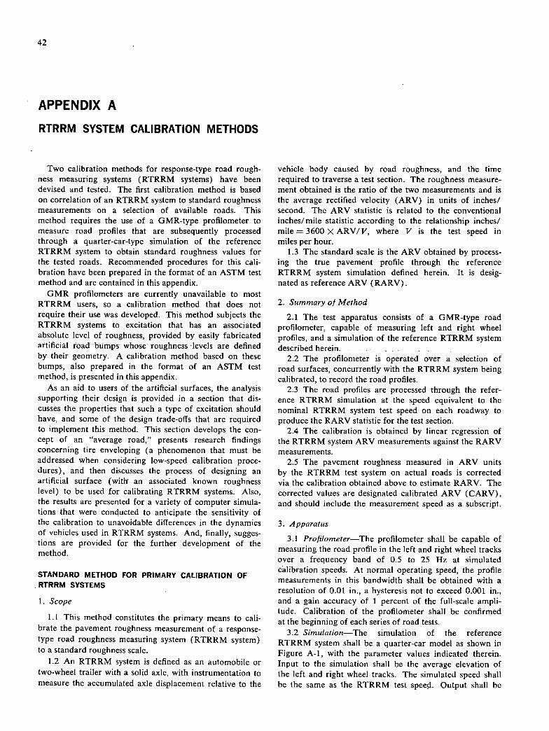
42

APPENDIX A

RTRRM SYSTEM CALIBRATION METHODS

Two calibration methods for response-type road rough-ness measuring systems (RTRRM systems) have been devised and tested. The first calibration method is based on correlation of an RTRRM system to standard roughness measurements on a selection of available roads. This method requires the use of a GMR-type profilometer to measure road profiles that are subsequently processed through a quarter-car-type simulation of the reference RTRRM system to obtain standard roughness values for the tested roads. Recommended procedures for this cali-bration have been prepared in the format of an ASTM test method and are contained in this appendix.

GMR profilometers are currently unavailable to most RTRRM users, so a calibration method that does not require their use was developed. This method subjects the RTRRM systems to excitation that has an associated absolute level of roughness, provided by easily fabricated artificial roadbunlpswhose roughness levels are defined by their geometry. A calibration method based on these bumps, also prepared in the format of an ASTM test method, is presented in this appendix.

As an aid to users of the artificial surfaces, the analysis supporting their design is provided in a section that dis-cusses the properties that such a type of excitation should have, and some of the design trade-offs that are required to implement this method. This section develops the con-cept of an "average road," presents research findings concerning tire enveloping (a phenomenon that must be addressed when considering low-speed calibration proce-dures), and then discusses the process of designing an artificial surface (with an associated known roughness level) to be used for calibrating RTRRM systems. Also, the results are presented for a variety of computer simula-tions that were conducted to anticipate the sensitivity of the calibration to unavoidable differences in the dynamics of vehicles used in RTRRM systems. And, finally, sugges-tions are provided for the further development of the method.

STANDARD METHOD FOR PRIMARY CALIBRATION OF RTRRM SYSTEMS

1. Scope

1.1 This method constitutes the primary means to cali-brate the pavement roughness measurement of a response-type road roughness measuring system (RTRRM system) to a standard roughness scale.

1.2 An RTRRM system is defined as an automobile or two-wheel trailer with a solid axle, with instrumentation to measure the accumulated axle displacement relative to the

vehicle body caused by road roughness, and the time required to traverse a test section. The roughness measure-ment obtained is the ratio of the two measurements and is the average rectified velocity (ARV) in units of inches/ second. The ARV statistic is related to the conventional inches/mile statistic according to the relationship inches! mile - 3600 X ARV/V, where V is the test speed in miles per hour.

1.3 The standard scale is the ARV obtained by process-ing the true pavement profile through the reference RTRRM system simulation defined herein. It is desig-nated as reference ARV (RARV).

Summary of Method

2.1 The test apparatus consists of a GMR-type road profilometer, capable of measuring left and right wheel profiles, and a simulation of the reference RTRRM system described herein.

2.2 The profilometer is operated over a selection of road surfaces, concurrently with the RTRRM system being calibrated, to record the road profiles.

2.3 The road profiles are processed through the refer-ence RTRRM simulation at the speed equivalent to the nominal RTRRM system test speed on each roadway to produce the RARV statistic for the test section.

2.4 The calibration is obtained by linear regression of the RTRRM system ARV measurements against the RARV measurements.

2.5 The pavement roughness measured in ARV units by the RTRRM test system on actual roads is corrected via the calibration obtained above to estimate RARV. The corrected values are designated calibrated ARV (CARV), and should include the measurement speed as a subscript.

Apparatus

3.1 Profilometer—The profilometer shall be capable of measuring the road profile in the left and right wheel tracks over a frequency band of 0.5 to 25 Hz at simulated calibration speeds. At normal operating speed, the profile measurements in this bandwidth shall be obtained with a resolution of 0.01 in., a hysteresis not to exceed 0.001 in., and a gain accuracy of 1 percent of the full-scale ampli-tude. Calibration of the profilometer shall be confirmed at the beginning of each series of road tests.

3.2 Simulation—The simulation of the reference RTRRM system shall be a quarter-car model as shown in Figure A-i, with the parameter values indicated therein. Input to the simulation shall be the average elevation of the left and right wheel tracks. The simulated speed shall be the same as the RTRRM test speed. Output shall be

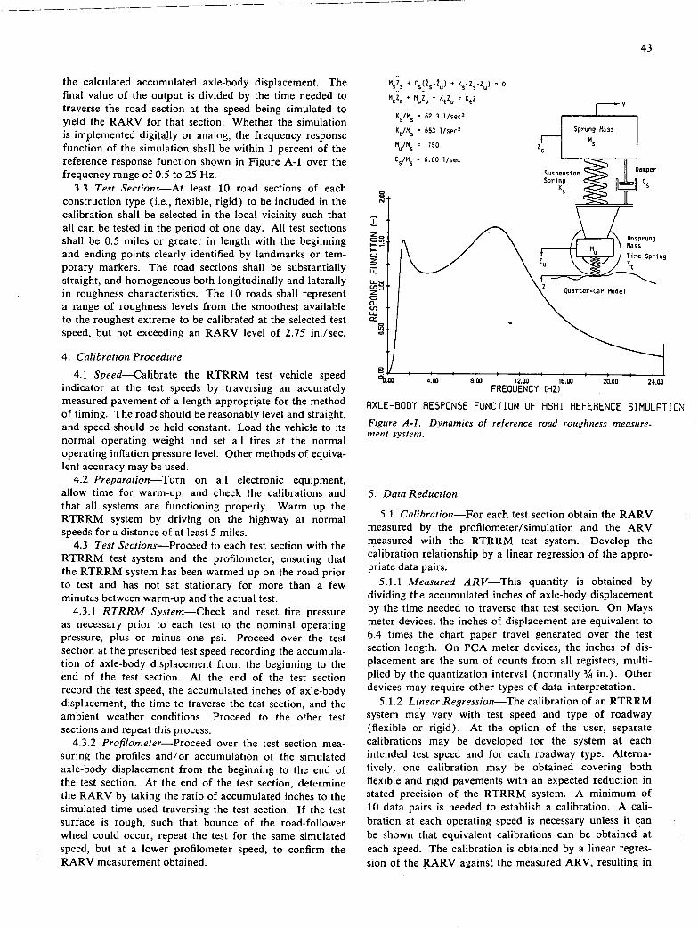
4.00 8.00 12.00 16.00 2010 24.00 FREQUENCY (HZ)

43

the calculated accumulated axle-body displacement. The final value of the output is divided by the time needed to traverse the road section at the speed being simulated to yield the RARV for that section. Whether the simulation is implemented digitally or analog, the frequency rcsponsc function of the simulation shall be within 1 percent of the reference response function shown in Figure A-i over the frequency range of 0.5 to 25 Hz.

3.3 Test Sections—At least 10 road sections of each construction type (i.e., flexible, rigid) to be included in the calibration shall be selected in the local vicinity such that all can be tested in the period of one day. All test sections shall be 0.5 miles or greater in length with the beginning and ending points clearly identified by landmarks or tem-porary markers. The road sections shall be substantially straight, and homogeneous both longitudinally and laterally in roughness characteristics. The 10 roads shall represent a range of roughness levels from the smoothest available to the roughest extreme to be calibrated at the selected test speed, but not exceeding an RARV level of 2.75 in./sec.

4. Calibration Procedure

4.1 Speed—Calibrate the RTRRM test vehicle speed indicator at the test speeds by traversing an accurately measured pavement of a length appropri$e for the method of timing. The road should be reasonably level and straight, and speed should be held constant. Load the vehicle to its normal operating weight and set all tires at the normal operating inflation pressure level. Other methods of equiva-lent accuracy may be used.

4.2 Preparation—Turn on all electronic equipment, allow time for warm-up, and check the calibrations and that all systems are functioning properly. Warm up the RTRRM system by driving on the highway at normal speeds for a distance of at least 5 miles.

4.3 Test Sections—Proceed to each test section with the RTRRM test system and the profilometer, ensuring that the RTRRM system has been warmed up on the road prior to test and has not sat stationary for more than a few minutes between warm-up and the actual test.

4.3.1 RTRRM System—Check and reset tire pressure as necessary prior to each test to the nominal operating pressure, plus or minus one psi. Proceed over the test section at the prescribed test speed recording the accumula-tion of axle-body displacement from the beginning to the end of the test section. At the end of the test section record the test speed, the accumulated inches of axle-body displacement, the time to traverse the test section, and the ambient weather conditions. Proceed to the other test sections and repeat this process.

4.3.2 Profilometer—Proceed over the test section mea-suring the profiles and/or accumulation of the simulated axle-body displacement from the beginning to the end of the test section. At the end of the test section, determine the RARV by taking the ratio of accumulated inches to the simulated time used traversing the test section. If the test surface is rough, such that bounce of the road-follower wheel could occur, repeat the test for the same simulated speed, but at a lower profilometer speed, to confirm the RARV measurement obtained.

M5Z5 + C5 (25_2) + K5(Z5_Z) 0

M5Z5 +MuZu + KtZU KtZ

Sprung M233 I 653 i/spr2

= 62.3 1/sec2

(t/M5

:-j

M5 MU/MS = . 150 Zs

6.00 i/Sec

uspension

II Damper

Spring JL Cs KS

I—I—

(2 z LL

LU2 (I, -

a- U, LU

U,

5. Data Reduction

5.1 Calibration—For each test section obtain the RARV measured by the profilometer/simulation and the ARV measured with the RTRRM test system. Develop the calibration relationship by a linear regression of the appro-priate data pairs.

5.1.1 Measured ARV—This quantity is obtained by dividing the accumulated inches of axle-body displacement by the time needed to traverse that test section. On Mays meter devices, the inches of displacement are equivalent to 6.4 times the chart paper travel generated over the test section length. On PCA meter devices, the inches of dis-placement are the sum of counts from all registers, multi- plied by the quantization interval (normally in.). Other devices may require other types of data interpretation.

5.1.2 Linear Regression—The calibration of an RTRRM system may vary with test speed and type of roadway (flexible or rigid). At the option of the user, separate calibrations may be developed for the system at each intended test speed and for each roadway type. Alterna-tively, one calibration may be obtained covering both flexible and rigid pavements with an expected reduction in stated precision of the RTRRM system. A minimum of 10 data pairs is needed to establish a calibration. A cali-bration at each operating speed is necessary unless it can be shown that equivalent calibrations can be obtained at each speed. The calibration is obtained by a linear regres-sion of the RARV against the measured ARV, resulting in

RXLE-BODY RESPONSE FUNCTION OF HSRI REFERENCE SIMULRTION

Figure A-i. Dynamics of reference road roughness measure-rnent system.

44

an equation of the form: RARV = Cl + C2 X ARV. The standard error, with the units inches/second, is calculated along with the regression equation and recorded with the calibration as an indication of its accuracy.

The calibration is recorded in the form of the foregoing derived equation, substituting the letters "CARV" for "RARV." The symbol CARV then denotes the calibrated ARV estimate of the reference ARV, based on measure-ments made with that system in subsequent road tests.

The calibration is identified by recording the date, RTRRM test system, tire inflation pressure, profilometer/ simulation system, actual and indicated test speed, pave-ment type(s), ambient weather conditions, and standard error. The calibration may be plotted on rectilinear graph paper as a straight line relating CARV to measured ARV for ease in subsequent use.

5.2 Pavement Roughness Measurement—The calibra-tion obtained above is used to convert on-road ARV rough-ness measurements to CARV units Because RTRRM systems may have varying degrees of sensitivity to test speed, pavement type, and ambient temperature, calibra-tions should be performed frequently to identify the particular sensitivities. The conversion of on-road measure-ments to CARV should then be obtained from the calibra-tion most closely related to the on-road conditions.

STANDARD METHOD FOR CALIBRATION OF RTRRM SYSTEMS ON AN ARTIFICIAL SURFACE

1. Scope

1.1 This method provides a means to calibrate the pavement roughness measurement of a response-type road-roughness measurement system (RTRRM system) to a standard roughness scale.

1.2 An RTRRM system is defined as an automobile or two-wheel trailer with a solid axle, with instrumentation to measure the accumulated axle displacement relative to the vehicle body caused by road roughness, and the time required to traverse a test section. The roughness measure-ment obtained is the ratio of the two measurements and is the average rectified velocity (ARV) in units of inches/ second. The ARV statistic is related to the conventional inches/mile statistic according to the relationship inches/ mile = 3600 x ARV/ V, where V is the test speed in miles per hour.

1.3 The standard scale is the ARV obtained by process-ing the true pavement profile through the reference RTRRM system simulation defined in the primary calibra-tion method. It is designated as reference ARV (RARV).

1.4 The method of calibrating on an artificial surface is an indirect method of calibrating that yields an estimate of the calibration that would be obtained by correlation of the subject RTRRM system against a profilometer/refer-ence RTRRM system simulation on a large sample of roads (i.e., the primary calibration). The calibration on an artificial surface is a means of estimating the primary calibration with sufficient accuracy to be useful in the absence of an available profilometer system, and is a means to monitor RTRRM system performance changes between primary calibrations due to changes in the vehicle, environ-

ment, etc. This calibration method does not include certain cffccts specific to vehicle speed and pavement types and hence has limited applicability.

Summary of Method

2.1 The test apparatus consists of a prepared surface fabricated from laminations of flat stock materials to yield a defined profile containing a relative roughness/wave number content that is related to the average properties of actual roads. The prepared surface is deployed on an existing base surface in a fashion to allow the RTRRM system (to be calibrated) to approach and drive over this surface with either both left and right wheels on the surface or just the wheels on the left or right side on the surface. The base surface is sufficiently smooth that the roughness level in the approach area, under the artificial surfaces, and in the departure area, is insignificant when compared to the roughness of the artificial surface.

2.2 The RTRRM system to be calibrated is driven five times over the test surface at each of five speeds by two methods as follows: (1) with both left and right wheels passing over the artificial surface simultaneously to yield a rough surface calibration point, and (2) with alternately the left wheels only and then the right wheels only passing over the artificial surface to yield a calibration point at a moderate roughness level. The inches of accumulated axle-body displacement, accrued during travel over the artificial surface and during the subsequent decay of vehicle bouncing after leaving the surface, are recorded.

2.3 A calibration plot for relating the subject RTRRM system to the standard scale is developed on rectilinear graph paper by plotting two points that are connected by a straight line. The two, points are: (1) the average measured roughness for all tests with both left and right wheels on the artificial surface corresponding to a given RARV value; and (2) the average measured roughness for all tests with the left and right wheels individually on the artificial surface corresponding to one-half the given RARV value.

2.4 The pavement roughness measured in ARV units by the subject RTRRM test system on actual roads is corrected via the calibration plot to obtain calibrated ARV (CARV) values.

Apparatus

3.1 Artificial Surfaces—The artificial surface is created by placing two basic profile patterns on an existing smooth pavement. The two patterns, designated A and B, are defined by the profile elevation views shown in Figure A-2. The surfaces must be of sufficient width to yield at least 12 in. (30 cm) of surface to the outside of the vehicle tires'to allow for tracking variations. The suggested width of the surface is 96 in. (2.44 m); or they may be con-structed of two pieces centered on the wheel tracks with a recommended width of at least 30 in. (76 cm).

3.2 Surface Installation—The artificial surface is pre-pared by construction and installation of profile segments as shown in the layout pattern of Figure A-3. The surface consists of four profile segments in the sequential series of

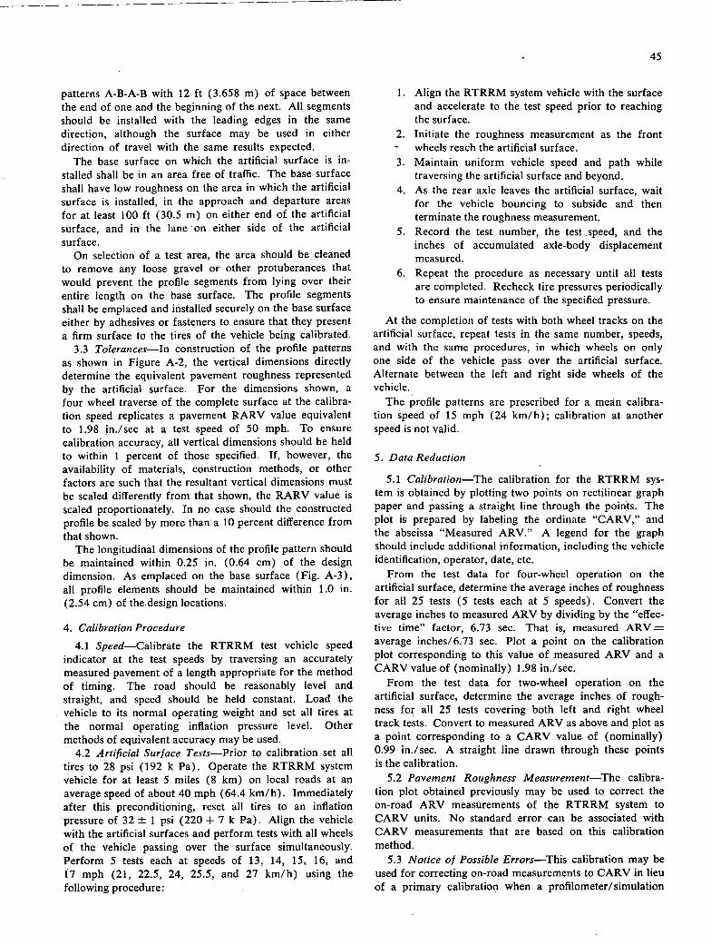
45

patterns A-B-A-B with 12 ft (3.658 m) of space between the end of one and the beginning of the next. All segments should be installed with the leading edges in the same direction, although the surface may be used in either direction of travel with the same results expected.

The base surface on which the artificial surface is in-stalled shall be in an area free of traffic. The base surface shall have low roughness on the area in which the artificial surface is installed, in the approach and departure areas for at least 100 ft (30.5 m) on either end of the artificial surface, and in the lane on either side of the artificial surface.

On selection of a test area, the area should be cleaned to remove any loose gravel or other protuberances that would prevent the profile segments from lying over their entire length on the base surface. The profile segments shall be emplaced and installed securely on the base surface either by adhesives or fasteners to ensure that they present a firm surface to the tires of the vehicle being calibrated.

3.3 Tolerances—In construction of the profile patterns as shown in Figure A-2, the vertical dimensions directly determine the equivalent pavement roughness represented by the artificial surface. For the dimensions shown, a four wheel traverse of the complete surface at the calibra-tion speed replicates a pavement RARV value equivalent to 1.98 in./sec at a test speed of 50 mph. To ensure calibration accuracy, all vertical dimensions should be held to within 1 percent of those specified. If, however, the availability of materials, construction methods, or other factors are such that the resultant vertical dimensions must be scaled differently from that shown, the RARV value is scaled proportionately. In no case should the constructed profile be scaled by more than a 10 percent difference from that shown.

The longitudinal dimensions of the profile pattern should be maintained within 0.25 in. (0.64 cm) of the design dimension. As emplaced on the base surface (Fig. A-3), all profile elements should be maintained within 1.0 in. (2.54 cm) of thedesign locations.

4. Calibration Procedure

4.1 Speed—Calibrate the RTRRM test vehicle speed indicator at the test speeds by traversing an accurately measured pavement of a length appropriate for the method of timing. The road should be reasonably level and straight, and speed should be held constant. Load the vehicle to its normal operating weight and set all tires at the normal operating inflation pressure level. Other methods of equivalent accuracy may be used.

4.2 Artijcial Surface Tests—Prior to calibration set all tires to 28 psi (192 k Pa). Operate the RTRRM system vehicle for at least 5 miles (8 km) on local roads at an average speed of about 40 mph (64.4 km/h). Immediately after this preconditioning, reset all tires to an inflation pressure of 32 ± 1 psi (220 + 7 k Pa). Align the vehicle with the artificial surfaces and perform tests with all wheels of the vehicle passing over the surface simultaneously. Perform 5 tests each at speeds of 13, 14, 15, 16, and 17 mph (21, 22.5, 24, 25.5, and 27 km/h) using the following procedure:

I. Align the RTRRM system vehicle with the surface and accelerate to the test speed prior to reaching the surface. Initiate the roughness measurement as the front

- wheels reach the artificial surface. Maintain uniform vehicle speed and path while traversing the artificial surface and beyond. As the rear axle leaves the artificial surface, wait for the vehicle bouncing to subside and then terminate the roughness measurement. Record the test number, the test speed, and the inches of accumulated axle-body displacement measured. Repeat the procedure as necessary until all tests are completed. Recheck tire pressures periodically to ensure maintenance of the specified pressure.

At the completion of tests with both wheel tracks on the artificial surface, repeat tests in the same number, speeds, and with the same procedures, in which wheels on only one side of the vehicle pass over the artificial surface. Alternate between the left and right side wheels of the vehicle.

The profile patterns are prescribed for a mean calibra-tion speed of 15 mph (24 km/h); calibration at another speed is not valid.

5. Data Reduction

5.1 Calibration—The calibration for the RTRRM sys-tem is obtained by plotting two points on rectilinear graph paper and passing a straight line through the points. The plot is prepared by labeling the ordinate "CARV," and the abscissa "Measured ARV." A legend for the graph should include additional information, including the vehicle identification, operator, date, etc.

From the test data for four-wheel operation on the artificial surface, determine the average inches of roughness for all 25 tests (5 tests each at 5 speeds). Convert the average inches to measured ARV by dividing by the "effec-tive time" factor, 6.73 sec. That is, measured ARV = average inches/6.73 sec. Plot a point on the calibration plot corresponding to this value of measured ARV and a CARV value of (nominally) 1.98 in/sec.

From the test data for two-wheel operation on the artificial surface, determine the average inches of rough-ness for all 25 tests covering both left and right wheel track tests. Convert to measured ARV as above and plot as a point corresponding to a CARV value of (nominally) 0.99 in./sec. A straight line drawn through these points is the calibration.

5.2 Pavement Roughness Measurement—The calibra-tion plot obtained previously may be used to correct the on-road ARV measurements of the RTRRM system to CARV units. No standard error can be associated with CARV measurements that are based on this calibration method.

5.3 Notice of Possible Errors—This calibration may be used for correcting on-road measurements to CARV in lieu of a primary calibration when a profilometer/simulation

46

Longitudinal Dimensions (ft)

tO to tO LI) 'tO 10' - It) In It) IC) It) CD 01 0

0 CD

l 1/2 I I

5/8 3/4' 7/6 1" 1 1/8 1 1/4'

LeadingEdge

PROFILE PATTERH A

'no . ' 0 01 ) Woo cD

Leading Edge PROFILE PATTERN B

Figure A-2. Elevation view of artificial surface profile patterns.

Longitudina1•Dirnensions(ft) ' -- ' --- ----

0 25 37' 59 1/2 71 j1/2 96 112

10811/2 131'

-- Tracks

Pattern Pattern Pa Pattern - - - A - - B

ttern B•

Leading Edge

Figure A-3. Layout plan for artificial surface profile elements.

is not available. However, the calibration accuracy is not assured. Insufficient damping in the rear suspension is a known cause of inaccuracy and is indicated when the average accumulated axle-body travel in a calibration exceeds the limit shown in Figure A-4. As shown, the limit depends on the level of meter hysteresis, which is found by measuring the difference in axle-body position when the meter enters a register (i.e., it "clicks") with motion in one direction, and leaves it with motion in the

other direction. The figure is valid for a surface RARV value of 1.98 in./sec; if the actual surface has a different RARV value, the ordinate should be rescaled accordingly.

Ultimately, the calibration obtained with this method may in some cases exhibit a systematic difference from that obtained in a primary calibration. Hence it should be used as a secondary calibration prior to, or between, primary calibrations. At such time that a primary calibration is obtained, the secondary calibration should be performed

47

concurrently to establish an individual "effective time" factor for each RTRRM system. This calibration does' not compensate for the effects of tire/wheel nonuniformities which strongly influence roughness measurements of smooth roads, such as new pavement constructions. Hence the calibration is not valid for road surfaces with CARV values less than 1.0 in./sec.

DEVELOPMENT OF ARTIFICIAL SURFACE

CALIBRATION METHOD

The calibration method presented in the preceding sec-tion follows the basic notion of calibrating an instrument by using the instrument to measure a standard unit of rough-ness. Because this approach presumes the existence of a standard unit of measure, the first step in the development of this method was the definition of a "standard road" that could provide the same calibration as the primary profilometer method presented earlier. The fabrication of a standardized surface is simplified if the calibration speed is reduced, such that the surface provides excitation at low speed that is typical of real roads being traversed by RTRRM systems at their normal operating speeds. The advantages are that the surface does not have to be as long and also that background roughness deriving from the underlying surface and from fabrication imprecision is easier to maintain at negligible levels. In effect, this is accomplished by compressing the profile in proportion to the ratio: (calibration speed)/(simulated operating speed).

The pneumatic tire is, however, unable to completely respond to changes in pavement elevation if they occur within distances that are comparable to the length of the contact patch between tire and pavement. Small surface features are "enveloped" by the tire, resulting in less force being transmitted to the vehicle. If the calibration speed is too low, the tire enveloping will attenuate too much of the roughness for the calibration to be valid. Thus the calibra-tion must be based on an adequate understanding of tire enveloping as well as on an understanding of the properties of normal roads. Accordingly, the phenomenon of tire enveloping was investigated, and the findings are presented in this section.

The actual design of an artificial surface used to calibrate RTRRM systems is the result of a number of trade-offs. The main concern during this project was to develop a surface that was easy and cheap to fabricate and to, devise a calibration method that was simple to follow and required no auxiliary instrumentation other than the road meter in the RTRRM system. As a result, the calibration method is subject to errors. Because of this, and the fact that the method has not been fully demonstrated in the field, some of the properties of the bumps are described to aid those users of RTRRM systems who might further develop the calibration methodology. Also, suggestions are made for the immediate direction that the further development should follow.

Properties of the Standard Road

Pavement elevation changes randomly along the length of most roads, requiring that descriptions of profile be

16

UNACCEPTABLE 15

14

Worse 13

12 ACCEPTABLE

11

10

8

statistical. In the past 20 years, spectral density functions have been found to be useful descriptors of highway and airfield runway pavements. The spectral density of an individual pavement section is generally unique, but when the spectral densities of a large number of roads are compared, they are seen to have similar shapes. The

- uniqueness of the spectral density of any given section of pavement is the reason that measurements made with different RTRRM systems do not agree perfectly, and why a large number of roads must be included in an on-road calibration. (On the other hand, the commonality between spectral densities of different pavement sections is the underlying reason that even dissimilar roughness measure-ments are correlated.) A calibration could be performed with just two surfaces if both were known to have only "average" properties and none of the unique features common to real roads which bias the calibration. Clearly the development of an artificial surface for calibration of RTRRM systems begins with the question, What is the spectral density of the average road?

Analytic expressions have been suggested by various researchers to use as a road model, for calculations, when measuredprofiles are not available. Houboult (25) sug-gested a model for airfield runways that is the most well-known road model and is defined as

Gz(v) = Go/v2 (A-i)

where Gz(v) is the (model) road spectral density, v is wave number (wave number= 1/wavelength), and Go, the sole parameter in the model, is a scaling factor that indicates the level of roughness. As more highway pave-ments were profiled, it became apparent that real road spectral densities have higher amplitudes at low wave numbers than predicted by the model. More recent models that have been suggested have included additional parame-ters to provide the capability for better matching measured spectral densities. But parameter values that allow..the models to represent average roads have not been estab-

0 .01 .02 .03 .04 .05 .06 .07 .08 .09 .10 .11 .12 .13 Meter Hysteresis (in)

Figure A-4. Shock absorber acceptability criterion.

48

.001 .01 .02 .1 1.0

Wave Number (cycle/ft)

Figure A-5. Normalized spectral densities of European con-crete roads.

1 .01 .05 .1 Wave Number (cycle/ft)

Figure A-6. Normalized spectral densities of European bi-tuminous roads.

lished. A suitable model should have just one parameter that establishes the roughncss, and the model should be validated by comparison with a large number of measured spectral densities. Given that highway personnel have traditionally differentiated between roughness measure-ments of flexible and rigid pavements, it is likely that separate models are needed for different construction types.

Figures A-S and A-6 show measured spectral densities of a number of European roads (26). The figures show slope spectral densities rather than elevation spectral densi-ties, because slope spectral densities do not change as much with wave number and peculiarities of individual spectra are thus easier to distinguish. Each measured curve was normalized (rescaled) in the figures to better show the common shape of the different curves. The heavy black lines depict an analytic spectral density function that was selected to best match the measured curves and define the average road model. The equation of each line is

Gz'(v) = Go[1 + (vo/v) 2] (ft/ft) 2ft/cycle (A-2)

The only difference between the models for rigid and flexible pavements is the value given to the parameter vo; a value of 0.02 cycle/ft is suggested for rigid constructions and a value of 0.05 cycle/ft is suggested for flexible construction. No trend is apparent that would indicate that the shape of the model spectral density should be different for smooth and rough roads; thus the single equation is offered for all levels of roughncss that were included in the survey. The model was found to also agree with measured spectra for Texas roads (27) and with the 18 Ann Arbor roads profiled during the Correlation Program.

When a road is traversed by a vehicle, it is perceived as a moving elevation. A standard calibration excitation should provide the same input to the RTRRM system vehicle as a road with properties specified by the foregoing equation, when said road is traversed at the normal RTRRM system measurement speed. On the basis of the transformations in Appendix C, the spatial spectral density of the calibration surface should be

Gz'(v) = GoC[1 + (Cvo/v) 2] (ft/ft) 2ft/cycle (A-3)

where C is the ratio of the simulated measurement speed to the calibration speed.

Tire Enveloping

Background

All of the forces that act on a vehicle in response to road roughness must be transmitted by the pneumatic tires, starting at the contact patch between tire and pavement. Although it is true that a tire acts much like a linear spring when the entire contact patch area is moved up and down, the force transmissibility actually varies throughout the contact patch. Thus, when the tire rolls over a bump or other pavement feature, the force transmitted to the spindle changes with the position of the bump within the contact patch. Figure A-7 illustrates the relationship between vertical spindle force and longitudinal position, when the tire is rolled over a very small cleat that extends across the width of the contact patch (perpendicular to the direction of travel) but is narrow compared to the length of the

20

10

-10

S..

49

contact patch. Lippman (28) has shown that tire envelop-ing can be treated as a linear behavior by successfully predicting force responses to various cleat shapes from the force responses to simple step inputs. (The response shown here would be predicted by adding the response to a positive step input with the response to a negative step input, with the two edges of the steps separated by the width of the cleat.)

Because the tire linearly relates spindle force to displace-ment throughout the contact patch, the simple concept of the tire as a linear spring need not be abandoned; rather it can be supplemented by the addition of a separate model of the contact patch enveloping. The displacement seen by the simple tire spring would still be a single-valued eleva-tion, but instead of being the pavement elevation at the center of the contact patch, it would be a weighted average of the profile under the entire contact patch. This weight-ing function can be measured by rolling the tire over a cleat narrow enough to approximate an impulse function input, as illustrated in the figure. (A more precise way of measuring the weighting function is by rolling the tire over a step, and then differentiating the response, because the derivative of a step input is an impulse function with a magnitude exactly equal to the height of the step.)

Tire enveloping can also be characterized as a wave number response function to better illustrate how the phenomenon affects RTRRM system calibration. The wave number response function is equivalent to a spatial fre-quency response function, obtained by calculating the Fourier transform of the weighting function. Figure A-8 shows the wave number response function calculated from the weighting function shown in the previous figure. The gain of the function is scaled to the unity for a wave num-ber of zero (a flat surface), under wIich condition changes in vertical spindle force are simply the result of the tire spring rate. But for increasing wave numbers, the envelop-ing function attenuates the input, such that the amplitude of variations in the vertical force will be less than predicted by the tire spring rate. And, at certain wave numbers, the enveloping completely attenuates the input such that no force variations would be observed if the tire were rolled over a sinusoidal surface having the "nodal" wave number indicated in the figure.

An artificial surface should not be designed to contain excitation vital for a valid calibration at wave numbers near the first node in the tire enveloping function. Ideally, all of the significant excitation should be at wave numbers that are low enough that the enveloping does little to attenuate the input. Alternatively, the input can be boosted at wave numbers near the first node, anticipating the attenuation. Thus the vehicle is ultimately given the proper excitation which corresponds to traversing an average road at the normal RTRRM system measurement speed.

The little published information on tire enveloping is not adequate to quantify the enveloping mechanism to the extent needed for proper design of a low-speed artificial surface for RTRRM system calibration. Measuring the weighting functions or wave number response- functions for a selection of tires -was beyond the scope of the re-search, but analysis of the enveloping phenomenon revealed

Distance S

Figure A-7. Illustration of tire envelopment.

1.0

C

1st Nodal Wave Number

Wave Number

Figure A-8. Fourier transform of weighting function shown in Figure A-7.

50

that the necessary information could be obtained with relatively few tests.

Tire Enveloping Tests

A tire rolling over a pavement irregularity generates vertical force that is perceived by the vehicle as a function of time. The weighting function and wave number response function, shown in Figures A-7 and A-8, are seen as functions of time and frequency, and are related to the spatial functions by the speed of the vehicle. The first nodal wave, number needs to be established to ensure that the calibration speed is selected to keep the corresponding frequency above the effective response limit of RTRRM systems.

Accordingly, a series of tests was designed and conducted to locate this node. The Highway Safety Research Institute test vehicle (1976 Pontiac station wagon) was instru-mented with necessary recording equipment, along with an accelerometer mounted on the rear axle, near the right-hand wheel. The car was then driven over small bumps, such as welding rods and pieces of angle iron attached to the pavement. The resulting axle motion was the combined result of the dynamic response to the bump and pavement and of the attenuation of the excitation due to tire envelop-ing. The signal from the accelerometer was processed by a real-time spectrum analyzer to determine the frequency cuittetil Uf the axle motion.

A number of tests were conducted, with speed (measured with a fifth wheel) and tire pressure varied. In all of the resulting frequency response plots, a node was evident. The node was seen to be at the same wave number when only the test speed was varied—evidence that it was caused by tire enveloping. As Figure A-9 shows, the nodal wave number was sensitive to tire pressure; hence, a (hot) tire pressure of 32 psi was selected and maintained for RTRRM system vehicles during calibration. (This corresponds approximately to a cold tire pressure of 28 psi.) At 32 psi, the nodal wavelength is 0.95 ft.

Tire Enveloping Model

A model of the tire-enveloping attenuation up to the first nodal wave number was needed for analysis and design of the artificial bumps. The simple model of a constant weighting function shown in Figure A-10 proved sufficient. In the model, the sensitivity of the tire to pavement irregu-larities is uniforñ'i for a certain length and zero elsewhere. The figure also shows the wave number response function that is associated with this assumed weighting function. The advantage of this model is that it is completely defined by a single parameter—the weighting function length—which is also the first nodal wavelength.

Analyses were made to estimate the magnitudes of errors that could be expected from using this model in lieu of the exact wave number response function. Published data indicate that a much better model of the tire-enveloping weighting function would be the difference between two uniform weighting functions. Figure A-il compares the two models with a real tire (28) by showing the vertical force resulting when the tire is rolled over a step input.

30

COD

- - Michelin 7815-R

20 Cib 0 Welding Rod

0 Angle Iron

10

0

90 Ii.. : CO

BOI 22 24 26 28 30 32 34 36 38 40

Tire Pressure (psi)

Figure A-9. Measured modal wavelengths.

l/Lc

0 _L/2 0 L/2

Distance

1.0

Sin(:vL)

l/Lc 2/Lc

Wave Number.

Figure A-b. Simple tire enveloping model.

The figure also shows the three weighting functions and the corresponding wave number response functions. Note that the more complex model requires three parameter values; thus perfect agreement between the two models is impossible. The fiequency response functions for a variety of parameter combinations were calculated and compared with the simple model. It was found that when the correct nodal wavelength is provided to the simple model, there is good agreement for wave numbers below the first node, as shown by the example in Figure A-il; accordingly, the,

C 0

0

a, C

4_I

a)

0

51

Complex Model

Simple Model

esntative eprTire

Distance

p 'o

A i—Complex Model

Representative Tire

Distance

ple

Tire

Sim

\dej~Representative

c 0m Model

1st Node\

Wave Number

Figure A-il. Comparison of two tire-enveloping models with representative ,neasurement.

simple model was used to predict tire-enveloping effects when needed during the project. (Agreement between the models suffers at wave numbers that are higher than the first node, but this wave number range has little effecLon RTRRM system performance.)

Design of Artificial Bumps

The artificial surface that was developed was intended to simulate a rough bituminous pavement being traversed at 50 mph. On the basis of the tire-enveloping data, a calibra-tion speed of 15 mph was selected. At this speed, the first node is at 23 Hz, which frequency is generally aboye the frequency range that affects RTRRM system measure-ments. The main consideration was keeping the attenuation less than 50 percent for frequencies less than 15 Hz, which resulted in the minimum speed of 15 mph. Still, 50 percent is a significant attenuation. Accordingly, the model road spectral density function was divided by the tire enveloping wave number response function for wave numbers up to 0.75, thereby boosting the high wave number roughness to compensate for the increased tire enveloping effects at the

low calibration speed. The road model shows large spectral density amplitudes at very low wave numbers, so the low frequency end was limited for wave numbers less than 0.023 cycle/ft, a value that corresponds to 0.5 Hz and is below the response limit of RTRRM system vehicles.

A spectral density function contains no phase informa-tion, and as a result any number of profiles could be con-structed to match the specified spectral density. A number of profiles were generated on the computer by summing a series of sine waves with very small amplitudes and with phase angles set randomly.

To simplify the task of fabricating an artificial surface, the different surface profiles generated on the computer were examined for sections that could be created by placing bumps on an existing smooth pavement. This required that the profile begin and end at a minimum elevation. It was also necessary that the roughness be more-or-less uniformly distributed over its length. For initial tests, a total length of 60 ft was desired. For ease of handling, candidate sections that could be provided by two bumps, 20 to 30 ft long, placed on an existing flat pavement were preferred. To further simplify the task of fabricating the bumps, the different candidate sections were quantized to changes in elevation of 1/8 in., so that they could be constructed from plywood and masonite or other flat stock materials.

An unwanted result of the modifications of the computer-generated surfaces is that the, actual spectral density of the artificial bumps does not match the design spectral density. In effect, the spectral density quality has been traded off to provide a bump design that is easier for the RTRRM system user to deal with. A variety of simple bumps designed as previously described were analyzed to select the pair that had a spectral density closest to the original design.

Preliminary testing, with just two bumps, showed that measurement precision was a problem. The source of this problem was the small amount of axle-body travel accumu-lated in a single pass together with the quantization levels in commercial road meters. Accordingly, a second set of bumps was fabricated to double the magnitude of the measurements from the road meters. However,' a random error still exists; thus the calibration procedure suggested in the previous section requires a number of passes to average out this error. More bumps could be added by users performing daily calibration checks in order to achieve a good calibration with fewer passes. Note that if a longer artificial surface is anticipated from the start, a larger set of unique bumps could be designed which would match the design spectral density better than the two bumps defined in Figure A-2.

Properties of the Artificial Bumps

Figure A-12 compares the actual spectral density of the artificial bumps with the design spectral density. Compar-ing this figure with Figures A-S and A-6 indicates that the artificial bumps deviate less from the average road curve than do most individual roads, although it is also clear that the match is not perfect. The notable peculiarities are that the bumps provide too much excitation at wave .numbers corresponding to frequencies of 0.7, 6, 11, and 13 Hz

w

(Note: Frequencies shown are for 15 mph)

' Reference Spectral vt Density

2.4 Hz 6 Hz 11 Hz 13 Hz

I \

Artificial Surface

'-.J....-4.5 Hz ' /

(Compensation for Tire Enveloping)

2 3 456789' txUi 2 Wave Number (cycle/ft) lxlO

52

Figure 4-12. Spectral densi:yof artificial surface.

(at 15 mph). But the proper excitation is providednear the body resonance of RTRRM system vehicles (1 to 1.5 Hz), and the excesses near the axle resonance are compensated by less excitation at adjacent frequencies also near the axle responance. To minimize the effects of these imperfections, the suggested calibration procedure requires testing at several speeds to effectively "smear" the peaks and troughs in the spectral density together.

The actual response of the HSRI reference to the arti-ficial bumps is shown in Figure A-13 (with the simulation modified to include the tire-enveloping model). The figure also breaks down the total simulated inches of axle-body travel as averaged over speeds of 13, 14, 15, 16, and 17 mph. These values can be used to calculate the accumu-lated inches that would be simulated for a different number of bumps, with the relation:

Inches of travel = 6.80 + (n-i) X 6.54 (A-4)

where n is the number of sets of bumps used (all spaced at 12-ft intervals). Thus, when two sets are used, as specified in the previous section, the HSRI reference should accumu-late 13.34 in. of axle-body travel. The design RARV value for the bumps is 1.98 in./sec. Inches of accrued axle-body travel that are measured with RTRRM systems are con-verted to ARV by dividing the measured value by an "effective time" that is found by ratioing the simulated inches of axle-body travel of the HSRI reference by the

RARV value. A time of 6.73 sec is obtained when two sets of bumps are used.

If the actual dimensions of the bumps differ from the specified geometry, the inches of travel, calculated by the foregoing equation, and the RARV value should be scaled accordingly. When only one side of the vehicle is driven over the bumps the RARV value should be reduced by 50 percent, but the "effective time" is unaffected.

RTRRM systems will display a speed sensitivity when operated on the bumps. Also, the measurements will be more sensitive to tire pressure than during on-road opera-tion, because the tire pressure affects not only the tire spring rate but also the tire-enveloping behavior. Table A-i gives the sensitivities of the HSRI reference simulation to both speed and the first nodal wavelength in the envelop-ing model described earlier to indicate the sensitivities that can be expected.

To estimate errors that could be obtained by calibrating RTRRM systems with vehicles that do not have response properties identical to the HSRI reference, a number of different vehicles were simulated on the bumps. Figure A-14 illustrates the response functions of the different simulated vehicles and also shows the measurements that would be obtained, along with the percent errors, if they were calibrated according to the method specified in the previous section. In general, the figure shows that the well-damped version of each of the five basic vehicle types is given a smaller error.

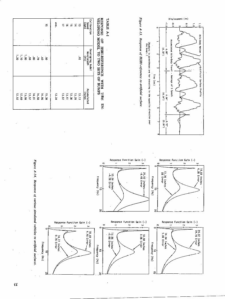
01 at -J CC 01 a to

C-, CD

, at 0. a)

0•

0 'C

CDCD •

tO .CDO -'0 0 0 0 0 0 0 0 01 C*CD - CO to 0- = 0 0. a,

0 Cc

11311) to to. a aol to to to to to toOC -'01001001)0W to a.' a to 113 - CD 113001 '.4-tOO.' 01 a 113-01 Olto 13W

C. CD 0.

tTlr1 1-1

V11 'S

CD

Wa,

- 17, ..a, .3

-1

I.

)isplacenent (in)

16 0

a,' c en—)

•

om 'C

a,.

00

C I-

- CC

0-' DCCC a to 1

1J C-, -I-

CD

0

0

FO CO

rD -n -S CD .0 = CD C 0 'C =

=

sponse Function Gain (-)

nse Function Gain 113 to

-1

2 C CD C

= N

,ponse Function Gai

Response Function Gain (-)

Response Function Gain (-) 0 - 113 to

0

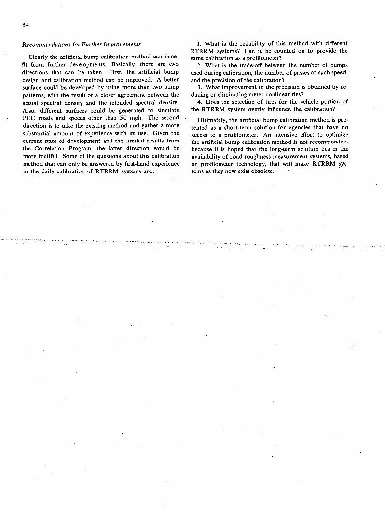
54

Recommendations for Further Improvements

Clearly the artificial bump calibration method can beiie-fit from further developments. Basically, there are two directions that can be taken. First, the artificial bump design and calibration method can be improved. A better surface could be developed by using more than two bump patterns, with the result of a closer agreement between the actual spectral density and the intended spectral density. Also, different surfaces could be generated to simulate PCC roads and speeds other than 50 mph. The second direction is to take the existing method and gather a more substantial amount of experience with its use. Given the current state of development and the limited results from the Correlation Program, the latter direction would be more fruitful. Some of the questions about this calibration method that can only be answered by first-hand experience in the daily calibration of RTRRM systems are:

What is the reliability of this method with different RTRRM systems? Can it be counted on to provide the same calibration as a profilometer?

What is the trade-off between the number of bumps used during calibration, the number of passes at each speed, and the precision of the calibration?

What improvement in the precision is obtained by re-ducing or eliminating meter nonlinèarities?

Does the selection of tires for the vehicle portion of the RTRRM system overly influence the calibration?

Ultimately, the artificial bump calibration method is pre-sented as a short-term solution for agencies that have no access to a profilometer. An intensive effort to optimize the artificial bump calibration method is not recommended, because it is hoped that the long-term solution lies in the availability of road roughness measurement systems, based on profilometer technology, that will make RTRRM sys-tems as they now exist obsolete.

APPENDIX B

55

CORRELATION PROGRAM

On October 8, 9, and 10, 1979, a Correlation Program was held at the Highway Safety Research Institute (HSRI) with the primary objective of assessing the accuracy with which in-use response type road-roughness measuring (RTRRM) systems could be calibrated. Six states partici-pated, yielding a total of 10 vehicles capable of 14 differ-ent measurements of pavement roughness. A new GMR-type profilometer system (Model 690D), recently built by K.J. Law for the State of West Virginia, was one of the participating systems and provided reference roughness values for local road sections that were used as test sites. The profilometer measured the elevations of both right-and left-hand wheel tracks, and besides simulating the ref-erence vehicle (described in App. A and Figure 22 in Chapter Two) the system stored the profiles on digital tape (with one elevation reading every 6 in.) for subsequent analyses. After the program was completed, these tapes were used ih èonjunction with computer models to produce measurements of various simulated systems, such as differ-ent reference configurations, CHLOE, etc.

Table B-i lists the participating agencies, their measure-ment systems, and also systems that were later simulated

using the profile tapes obtained by the West Virginia pro-filometer. One of the road meters, designated "electronic," was fabricated by HSRI during the research and is de-scribed at the end of this appendix.

The program was mainly concerned with evaluation of the artificial road bump and the primary profilometer cali-bration methods that are detailed in Appendix A. The first day of activity was devoted to calibration tests on the artificial road bumps. Speedometer and odometer calibra-tions were also performed. On the second day, the 10 vehicles convoyed to 24 preselected road sites at which on-road roughness measurements were made. The third day was used by each participant to reduce the artificial bump data to a calibration,, and then reduce the road test data. Some retesting was also conducted.

On-road roughness measurements were made in convoy fashion at preselected sites in the vicinity of Ann Arbor, Michigan. The sites included 19 bituminous surfaces rang-ing from very smooth to very rough. The remaining 5 surfaces were portland cement concrete slab construction ranging from new surfaces to older construction with con-siderable joint deterioration. The beginning and the end

TABLE B-I

ROAD ROUGHNESS MEASURING SYSTEMS EVALUATED IN THE CORRELATION PROGRAM

Vehicle Meter

Agency Model Suspension Tires Model Quantization Hysteresis Notes

Georgia DOT 1976 Ford Coil Spring Michelin Mays 0.10" 0.010 Car also had PCA Torino Wagon Delco Shocks HR78-14 Meter meter, not used

in_study

Mays Meter Coil Spring Michelin Mays 0.101, 0.027 Trailer Delco Shocks GR78-14 Meter

HSRI 1976 Pontiac Coil Spring Michelin Mays 0.10" 0.030 Station Wagon llnnroematic 215-156 Meter

Shocks

PCA Meter .125" 0.100" Roughness measured by surning counts (not_weighted)

Electronic Meter Hone None

Meter used LVDT transducer, was susceptible to CB interference

Kentucky DOT 1975 Plymouth Leaf Spring Goodyear Mays 0.10 0.040" PSI values determined

Wagon GR78-15 Meter

Profilometer Simulated BPR Roughometer Ideal" Data was not used Meter due to hardware

problem

Ohio DOT 1977 Ford Coil Spring 1178-14 Mays 0.101, 0.030 Data was notused LTD 11 "Heavy Duty Meter due to tire imbalance

Shocks"

Wisconsin 1976 Pontiac Coil Spring 8FG Mays 0.10" 0.023" DOT Catalina OEM "Heavy Duty" 11970-15 Meter

PCA Unknown Unknown Output of meter was Shocks

Meter "PSI," based on "PCA meter_statistic"

Michigan Profilometer Measured profile is

DOT ' processed to yield a Ride Quality lndeu (RQI)

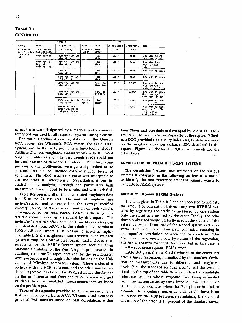
56

TABLE B-i

CONTINUED

Vehicle Meter

Agency Model Suspension Tires Model Quantization Hysteresis Notes

W. Virginia 1974 Oldsmobile Coil Spring Firestone Mays 0.101, 0.030" DOT, K.J. Law Cutlass Sedan 670-14 Meter Corp. and HSRI Profilometer Reference Vehicle

Simulation _________ Ideal Meter

.001" None Simulated dunn runs (real time

Profilometer Reference Vehicle Ideal .001" None Simulated from Digital Profile Tapes

Simulation Meter profile tapes later

Impala Ideal .001" None Used profile tapes Simulation Meter

Band Pass Filter Ideal .001" None Used profile tapes (0.8-15 Hz) Meter

Reference Vehicle Simulation

Simulated Mays Meter

.0011, 0.030" Used profile tapes Used 'average hysteresis effects

Reference Vehicle Simulation

. Simulated PCA Meter

.001' 0.100" Used profile tapes Used "average" hysteresis effects

Reference Vehicle Simulation

Envelop. Model

Ideal Meter

.001' None Used profile tapes -.

AASHO Profilo- .001" None Used profilometer meter Simulation (slope variance)

geometry from Fig. in (9), Used profile tape

of each site were designated by a marker, and a common test speed was used by all response-type measuring systems.

For various technical reasons, data from the Georgia PCA meter, the Wisconsin PCA meter, the Ohio DOT system, and the Kentucky profilometer have been excluded. Additionally, the roughness measurements with the West Virginia profilometer on the very rough roads could not be used because of damaged transducer. Therefore, com-parisons to the profilometer were generally limited to 18 surfaces and did not include extremely high levels of roughness. The HSRI electronic meter was susceptible to CB and other RF interference. Nevertheless it was in-cluded in the analysis, although one particularly high measurement was judged to be invalid and was excluded.

Table B-2 presents all of the uncorrected roughness data for 18 of the 24 test sites. The units of roughness are inches/second, and correspond to the average rectified velocity (ARV) of the axle-body motion of each vehicle, as measured by the road meter. (ARV is the roughness statistic recommended as a standard by this report. The inches/mile statistic often obtained from Mays meters can be calculated from ARV, via the relation inches/mile = 3600 X ARV/V, where V is measuring speed in mph.) The table lists the roughness measurements taken by each system during the Correlation Program, and includes mea-surements for the HSRI-reference system acquired from on-board simulation on the West Virginia profilometer. In addition, road profile tapes obtained by the profilometer were post-processed through other simulations on the Uni-versity of Michigan computer system. These included a recheck with the HSRI-reference and the other simulations listed. Agreement between the HSRI-reference simulations on the profilometer and from the tapes is excellent and validates the other simulated measurements that are based on the profile tapes.

Three of the agencies provided roughness measurements that cannot be converted to ARV. Wisconsin and Kentucky provided PSI statistics based on past correlations within

their States and correlations developed by AASHO. Their results are shown plotted in Figure 26 in the report. Michi-gan DOT provided ride quality index (RQI) statistics based on the weighted elevation variance, EV, described in the report. Figure B-i shows the RQI measurements for the 1-8 surfaces. - -

CORRELATION BETWEEN DIFFERENT SYSTEMS

The correlation between measurements of the various systems is compared in the following sections as a means to identify the best reference standard against which to calibrate RTRRM systems.

Correlation Between RTRRM Systems

The data given in Table B-2 can be processed to indicate the amount of correlation between any two RTRRM sys-tems by regressing the statistics measured by one system onto the statistics measured by the other. Ideally, the rela-tionship obtained would perfectly predict the statistic of the reference system from that of the second system and vice-versa. But in fact a random error still exists resulting in an imperfect correlation between the two systems. The error has a zero mean value, by nature of the regression, but has a nonzero standard deviation that in this case is also the root-mean-square (RMS) error.

Table B-3 gives the standard deviation of the errors left after a linear regression, normalized by the standard devia-tion of measurements due to different road roughness levels (i.e., the standard residual error). All the systems listed on the top of the table were considered as candidate reference systems whose responses are being estimated from the measurement systems listed on the left side of the table. For example, when the Georgia car is used to estimate the roughnes numerics that would have been measured by the HSRI-reference simulation, the standard deviation of the error is 19 percent of the standard devia-

0 1.0 2.0 3.0

Reference System ARV (in/sec)

Figure B-i. Comparison of Michigan RQI with reference ARV.

S

S

• . . • S

S S • S

S.

100

80

20

57

TABLE B-2

UNCORRECTED ROUGHNESS MEASUREMENTS FROM EACH SYSTEM ON THE 18 TEST SITES

Test Site Georgia HSRI W. Virginia Profilometer Tane HSRI Band Pass Ref. AASHO AASHO V Ky. Wis. W. Va. HSRI

o. Type (mpI) (ml.) Car Trailer Mays PCA Elect. jjg Ref. Ref. Impala Filter Mays PCA Env. /V PSI

1 Bit. 45 .81 1.53* 1.19* 1.51* 1.28* 1.81* 1.64* 2.31* 1.74* 1.92* 1.90* 2.91* 1.45* 1.58* 1.19* 1.85* 5.00** 2.41

2 Bit. 50 .84 1.07 0.88 1.10 0.82 1.31 1.13 1.49 1.08 1.31 1.32 1.83 1.02 1.04 0.72 1.30 2.50 3.34

3 Bit. 50 1.01 0.78 0.57 0.72 0.50 0.72 1.10 0.78 0.94 0.94 1.56 0.79 0.72 0.49 1 0.93 1.67 3.65

4 Bit. 45 1.30 1.26 0.99 1.24 0.76 1.61 1.29 1.88 1.39 1.65 1.65 2.54 1.29 1.29 0.89 1.60 • 4.47 2.61

5 Bit. 50 .90 1.07 0.71 0.96 0.67 1.18 0.96 1.50 1.42 1.26 1.29 2.27 1.03 1.03 0.72 1.26 2.82 3.22

7 PCC 50 1.01 1.46 1.24 1.53 1.14 1.71 1.44 1.88 1.81 1.85 1.82 2.57 1.42 1.47 1.07 1.77 5.12 2.59

8 Bit. 50 1.01 0.53 0.35 0.51 0.32 0.74 0.44 0.99 0.67 0.68 0.68 1.12 0.54 0.47 0.31 0.67 1.42 3.74

9 Bit. 50 1.05 0.44 0.25 0.39 0.19 0.78 0.36 1.06 0.43 0.57 0.58 0.98 0.48 0.39 0.24 0.57 1.29 3.79

10 PCC 50 1.01 1.92 1.61 2.18 1.64 2.29 2.06 , 2.49 2.39 2.26 2.24 3.09 1.75 1.83 1.35 2.18 5.59 2.19

11 Bit. 35 0.51 0.68 0.49 0.74 0.44 1.10 0.61 0.99 0.64 ' 0.88 0.85 1.24 0.67 0.63 0.32 0.83 1.95 3.54

12 Bit. 35 0.81 1.46 1.14' 1.50 1.11 1.65 1.61 1.82 1.58 1.74 1.78 2.49 1.40 1.44 1.00 1.70 4.69 2.53

13 Bit. 50 1.02 1.17 1.06 1.24 0.90 1.47 1.28 1.67 1.32 1.42 1.40 1.86 1.12 1.08 0.75 1.39 2.60 3.30

14 Bit. 50 ' 1.01 1.57 1.43 1.68 0.96 1.90 f.60 1.90 2.43 1.86 1.85 2.81 1.45 1.39 0.93 1.78 5.22 2.33

15 Bit. 50 1.50 1.89 1.42 1.85 1.26 2.15 1.79 2.18 2.15 1.96 1.96 3.06 1.47 1.61 1.18 1.92 3.54 2.95

19 Bit. 45 0.81 0.71 0.32 0.68 0.44 0.96 0.69 1 1.21 0.65 0.88 0.86 0.68 0.70 0.65 0.44 0.85 1.71 3.63

22 'PCC 50 0.91 1.42 1.13 1.38 0.96 1.68 1.35 1.89 1.53 1.64 1.64 2.35 1,25 1.25 0.85 1.60 3.11 3.43

23 PCC 50 1.04 0.99 0.78 0.93 0.61 1.18 0.90 1.32 1.03 1.14 1.15 1.56 0.93 0.85 0.56 1.13 2.61 3.64

24 PCC 50 1.06 1.10 0.92 1.01 0.60 1.31 0.97 1.58 1.39 1.50 1.46 2.04 , 1.14 1.03 0.67 1.42 3.90 3.10

ave 1.17 0.92 1.18 0.81 1.46 1.16 1.63 1.36 1.41 1.41 2.05 1.11 1.10 0.76 1.38 3.29 3.11

o 0.43 0.40 0.48 0.38 0.43 0.49 0.46 0.60 0.49 0.48 0.74 0.36 0.42 0.33 0.47 1.44 0.54

u/W 0.37 0.44 0.41 0.47 0.30 0.42 0.28 0.44 0.34 0.34 0.36 0.33 0.38 0.43 0.34 0.44 0.17

* Inches/Second x iOJ ft/ft rms

tion of the overall measurements. In this example, 3. percent (0.19 X 0.19 = 0.036) of the total variance of the estimated measurements is a random error, and the other 96.4 percent can be attributed to a correlation between the two systems (\/0.964 = 0.98 = correlation coefficient, r).

Most of the simulated systems involve linear vehicles, while real RTRRM systems employ vehicles that are known to be nonlinear. Therefore, a nonlinear regression was ex-pected to reduce the residual errors. Quadratic regressions

ere tried, but offered an improvement that was too slight to justify the higher order regression over the simpler linear regression. This observation may be due to the small sample size (18) and is not expected to apply in general. Future research that involves correlating RTRRM systems with known nonlinearities should consider higher order re-gressions, although linear regressions might again prove adequate.

Correlation with Proposed Reference Simulations

Table B-3 indicates that the proposed HSRI-reference simulation correlates nearly as well with all of the RTRRM systems as the best of the actual RTRRM systems, and better than most. Two other reference simulations were considered-the Impala and the band pass filter. The response functions for each are shown in Figure B-2. (Parameter values for these simulations are contained in Table C-2.) The Impala simulation, which has been im-plemented on profilometers in the past, is seen to be much

58

TABLE B-3

STANDARD RESIDUAL ERRORS AFTER LINEAR REGRESSION

Candidate Reference Sys tern

Georgia HSRI W. Virginia Profile Tapes

Ref. Impala Band Pass Filter Mays PCA

Ref. + env. /V P51* Measurement

System Car Trailer Nays PCA Elect.** Ky. Nays

Wis. Nays

W. a. Nays

HSRI Ref.

Georgia Car 0 .21 .16 .29 .17 .17 .28 .29 .19 .19 .32 .20 .18 .23 .17 .53 .54

Georgia Trailer .21 0 .20 .35 .23 .23 .36 .27 .21 .21 .35 .22 .27 .33 .21 .46 .48

SRI Nays .16 .20 0 .24 .15 .15 .32 .30 .22 .22 .39 .22 .22 .27 .22 .51 .48

IISRI PCA .29 .35 .24 0 .32_ .22 .32 .46 .31 .31 .45 .31 .24 .22 .30 .58 .56

HSRI Elec.** .17 .23 .15 .32 0 .20 .30 .34 .24 .24 .37 .27 .24 .30 .24 .55 .54

Kentucky Nays .17 .23 .15 .22 .20 0 .27 .35 .20 .20 .37 .19 .16 .20 .18 .53 .51•

Wisconsin Nays .28 .36 .32 .32 .30 .27 0 .41 .24 .24 .37 .28 .23 .21 .24 .52 .52

W. Virginia Nays .29 .27 .30 .46 .34 .35 .41 0 .31 .31 .34 .36 .40 .40 .32 .40 .36

Ave. .22 .27 .22 .31 .24 .23 .32 .35 .24 .24 .37 .25 .24 .27 .24 .51 .50

RNS Ave. .23 .28 .23 .32 .25 .24 .33 .35 .24 .24 .37 .25 .24 .28 .24 .51 .50

SRI Ref. .19 .21 .22 .31 .24 .20 .24 .31 0 .04 .28 .06 .11 .19 .42 .45

Note: Residual error = /li • r = correlation coefficient

*Only 50 mph data (13 runs)

**itted surface 3 (17 runs)

less damped than the reference suggested by HSRI. Hence, it has an exaggerated sensitivity to the portions of the overall roughness that excite the body and axle resonances. As a result of this "tuning" effect, this simulation exhibits large residual errors when correlated with other RTRRM systems, as seen in Table B-3, and is a poor choice for a reference.

Another, reference simulation that was considered is a simple band pass filter whose response function gain, shown in Figure B-2, is similar to a "maximally flat" quarter-car model, with large amounts of damping. Although the re-sponse function of the broad pass filter does not resemble that of the reference simulation or of measured vehicle response functions very closely, Table B-3 indicates that the band pass filter simulation correlates well with all of the participating RTRRM systems, and, furthermore, cor-relates extremely well with the reference simulation. This is further evidence that agreement between different RTRRM systems is improved by installing the stiffest shock absorbers on the vehicle that the user can find.

Effects of Meter Hysteresis on Correlation

The reference vehicle employs an "ideal" road meter, in that quantization and hysteresis effects are excluded. Because quantization introduces a random error (as speci-fied in App. C), there is clearly no reason to include this effect in the reference. But hysteresis introduces a more-or-less deterministic error that is a function of the ratio between the hysteresis level and the RMS axle-body dis-placement, as shown in Figure 14 in Chapter Two of the report. Although hysteresis is identified as an unwanted

1\

I' /\

I I HSRI

/

Reference

Impala

/

----- Band Pass Filter

.00 4.00 8.00 12.00 18.00 20.00 24.00

Frequency (liz)

Figure B-2. Response function gains of three possible reference simulations.

feature of current road meters that should be eliminated in the future, its existence is a fact that should not be com-pletely ignored. To address this effect, two levels of hyster-esis were added to the reference vehicle, as indicated in Table B-i. (Hysteresis and quantization act together to introduce a random error based on the unknown equi-librium position of the axle relative to the center quantiza-tion interval. This error was eliminated from the reference simulation by utilizing the average hysteretic losses defined by the solid line in Fig. 14.) The two levels correspond to measured levels in the Mays and PCA meter installed in the HSRI vehicle. Table B-3 demonstrates that, even though the participating RTRRM systems include meters with hysteresis, errors due to imperfect correlation are not reduced when hysteresis is added to the reference, and, additionally, residual errors are introduced between the reference simulations with and without hysteresis. A sig-nificant exception to this trend was the HSRI-PCA meter system, which included the highest level of meter hysteresis. In this case, the residual errors were significantly reduced, demonstrating that hysteresis is the main culprit in causing the residual errors with this system.

A final note on hysteretic effects is that the best correla-tion was between the well-damped reference and simple band pass simulations, neither of which included meter hysteresis. Ultimately, the precision obtainable from cali-brated RTRRM systems might be improved from the 20 percent residual errors shown for the well-damped systems (with 0.03 in hysteresis) to approximately half that, by eliminating meter hysteresis. (The electronic meter in-stalled in the HSRI vehicle and described at the end of this appendix had no hysteresis, but was prone to errors from CB interference that mitigated the improvements gained by eliminating the hysteresis. Table B-7 shows that when the 5 smoothest pavements having significant bias due to RE interference are excluded from the analysis, the electronic meter produces the least scatter.)

Tire-Enveloping Effects

Pneumatic tires tend to envelope features of the pave-ment that are small compared to the contact patch. The net result, described in detail in Appendix A, is that the force transmissibility of the tire is reduced for high wave numbers when wavelengths near the contact patch length. The proposed reference simulation assumes that the tire contacts the pavement at a single point, and therefore does not include the tire-enveloping effect. A tire-enveloping model was added to the HSRI-reference simulation to ex-amine the influence on the calculated RARV and the calibration obtained. Because of the relatively long dis-tance between samples on the profile tapes (6 in.) and 'the absence of anti-aliasing filtering, the effect of envelop-ing is not well quantified by these results. Nevertheless, the results merit presentation. Table B-2 indicates that when enveloping is added to the reference simulation, the measured ARV is reduced, with the reduction being greater on rougher roads. Table B-3 indicates that in some cases the correlation with other RTRRM systems is improved but that the improvement is minor and not really sufficient

to justify the extra complexity resulting from adding the enveloping to the reference simulation. The six rougher surfaces that are generally excluded from the Correlation Program results were profiled at low speed at a later time. The RARV calculated from the HSRI-reference on these surfaces generally exceeds those measured by actual RTRRM systems. The likely reason is the absence of the tire-enveloping effect in the simulation. It is suggested that the inclusion of a tire-enveloping model be considered in the event the reference simulation is to be used on roads with RARV measurements greater than 2.75 in./sec (ap-proximately 2.0 PSI). The moving average model, devel-oped in Appendix A, is a good approximate model when a tire contact length of 0.95 ft is used.

Correlation with CHLOE and PSI

Because of the major role of the AASHO (CHLOE) profilometer in the development of the pavement service-ability concept, slope variance numerics were prepared using a simulated CHLOE profilometer. Ideally, the CHLOE measures the angle between a short-wheelbase arm, 9 in. long, and the long-wheelbase trailer chassis, 25.5 ft long. This is exactly how the profile tapes were processed, using the average of the right- and left-hand track elevations. The proper regression form between an RTRRM system and the CHLOE slope variance, SV, at a given speed is quadratic (see App. C); hence, Tables B-2

and B-3 present numbers based on VSV for comparison to

the ARV measurements. Table B-3 shows the VSV statistic to be a poor reference for RTRRM systems—a conclusion that is predictable from the analyses in Appendix C in which it is found that only 50 percent of the SV derives from the portion of road roughness affecting the RTRRM measurements. The PSI figures displayed in the tables de-

rive from linear regressions with VSV developed in Yoder and Milhous (29). Different formulas are used for bitu-minous and PCC construction and exclude the additional measurements of cracking, rut depth, etc. that are required by the original AASHO study. (The variable log (SV +1) has also been used in the past for PSI regressions and has

about the same statistical significance as the VSV vari-

able—therefore, VSV was used in the tables because of

the underlying linear relation between VSV and ARV.) Correlations between ARV measurements and CHLOE-based PSI measurements are much poorer than correlations between different RTRRM systems measuring ARV, indi-cating that the PSI statistic is not a good choice for a calibration standard and that there is little utility in con-verting the ARV statistic to the PSI statisic. A similar conclusion was reached wih the RQI statistic measured by Michigan DOT. The RQI is ideally a linear function of ln(ARV), but the correlation between ARV and RQI was the same as the correlation between ln(ARV) and RQI—quantified by a standard error of 0.57. The main causes for the poor correlation are the difference in the wave number ranges of road roughness that contribute to each statistic and the fact that the Michigan system pro-files one wheel path, while the West Virginia machine pro-files both tracks.

60

CALIBRATION EFFECTIVENESS

Having established that the ARV produced by the HSRI-reference system (profilometer with quarter-car simula-tion), designated the RARV, constitutes a reasonable cali-bration standard, different methods for obtaining the cali-bration of an RTRRM system against the HSRI-reference can be evaluated.

Primary Calibration Against a Profilometer

The primary calibration curve for an RTRRM system is found simply by regressing RARV measures from a pro-filometer with HSRI-reference simulation against ARV measurements from the RTRRM system over a variety of roads. The regression curve is then used to correct the data to predict standard measurements that would have been made by the reference. Table B-4 gives all of the corrected roughness measurements for the 8 RTRRM sys-tems on the 18 test sites. The scatter is shown for each surface as the root-mean-square (RMS) error and as a relative error (ratio of the RMS error to the standard roughness measurement). Overall, the average RMS error is 0.11 in./sec, and the average percent error is 8.8 per-cent. Generally, the RMS error is more or less indepen-dent of roughness, and thus the percent error is greater on the smoother roads. Of the 18 test sites, only three result in bias crrors between the - standard and the average of 8 RTRRM systems that are greater than 0.10 in./sec. Hence it is concluded that the HSRI-reference does not discriminate for or against any simple category of roads. The scatter for each RTRRM system is given in Table B-3 (normalized by the 0.487 in./sec standard deviation

of the roughness measurements over the 18 test sites) in the HSRI-reference eoluinii. The scatter is given without being normalized in Table 5 of Chapter Two.

Calibration with Artificial Bumps

Measurements made during the artificial bump calibra-tion are summarized in Table B-5, and the calibration procedure is described in Appendix A. The average ac-cumulated inches per pass, over the 5 calibration speeds, was divided by an "effective time" of 6.73 sec for the rough surface, and 13.34 sec for the longer smooth sur-face, to yield two ARV values with units inches/second. These two ARV values are shown under the heading "Bump Cal" in the table. The plywood bumps have a design roughness of 1.98 in./sec and 0.99 in./sec for the rough and smooth versions, respectively, but because the thicknesses of the bumps, as fabricated, were greater than the design dimensions, the actual reference values were 2.08 in./sec and 1.04 in./sec. The calibration curve is made by plotting the reference values against the mea-sured values, and then connecting the two points with a strainght line. The regressions from the primary calibra-tion were used in conjunction with the reference values associated with the two surfaces to calculate the ARV values that should have been measured by each system on the two surfaces. These two values are given in the table under the heading "Prim. Cal." -

Discussion of Calibration Tests

One measure of the validity of this calibration method is the comparison of the ARV values in the Bump Cal

TABLE B-4

ROUGHNESS MEASUREMENTS AS CORRECTED FOR PRIMARY CALIBRATION

Test HSRI Georgia HSRI iy. Wisc. W. Va. RMS % RMS Site Ref. Car Trailer Mays PCA Elec. Ma s Ma s Mays Ave. Ref. -Ave. Error Error

1 1.92 1.81 1.74 1.74 1.98 1.81 1.89 2.12 1.71 1.85 .07 .16 8.3 2 1.31 1.31 1.37 1.34 1.43 1.28 1.39 1.28 1.20 1.32 -.01 .08 5.8 3 0.94 0.99 1.01 0.97 1.04 0.98 0.87 0.97 0.98 -.04 .06 6.5 4 1.65 1.51 1.50 1.48 1.35 1.60 1.54 1.68 1.44 1.51 .14 .17 10.3 5 1.26 1.31 1.17 1.20 1.24 1.15 1.22 1.29 1.46 1.25 .01 .10 8.3

7 1.85 1.73 1.80 1.76 1.81 1.71 1.69 1.68 1.76 1.74 .09 .10 5.6 8 0.68 0.71 0.75 0.76 0.82 0.68 0.70 0.76 0.88 0.75 -.07 .10 14.8 9 0.57 0.61 0.63 0.64 0.66 0.72 0.63 0.83 0.70 0.68 -.11 .13 23.0

10 2.26 2.24 2.73 2.40 2.42 2.32 2.30 2.31 2.21 2.30 -.04 .09 3.8 11 0,88 0.88 0.91 0.99 0.96 1.06 0.87 0.76 0.86 0.91 -.03 .09 10.2

12 1.74 1.73 1.68 1.73 1.78 1.64 1.86 1.62 1.59 1.70 .04 .10 5.8 13 1.42 1.42 1.59 1.48 1.52 1.45 1.53 1.46 1.39 1.48 -.06 .09 6.3 14 1.86 1.86 2.02 1.91 1.60 1.91 1.85 1.70 2.24 1.88 -.02 .20 10.5 15 1.96 2.21 2.01 2.08 1.96 2.17 2.04 1.99 2.02 2.06 -.10 .13 6.6 19 0.88 0.91 0.71 0.93 0.96 0.91 0.95 0.99 0.87 0.90 -.02 .09 10.0

22 1.64 1.69 1.67 1.62 1.60 1.67 1.60 1.69 1.55 1.63 .01 .05 3.1 23 1.14 1.22 1.26 1.17 1.17 1.15 1.16 1.10 1.16 1.17 -.03 .06 5.2 24 1.50 1.34 1.42 1.25 1.16 1.28 - 1.23 1.37 1.44 1.31 .19 .21 14.3

a 0.49 0.48 0.48 0.47 0.46 0.47 0.48 0.47 0.46 0.46 .08 .05 4.8

ave. .11 8.8

61

TABLE B-5

ARTIFICIAL SURFACE CAT.T1RATION RESULTS

Rough Surface - R (in) - Smooth Surface - S (in) Bump Cal Prim. Cal (in/sec) (In/sec) 13 14 15 16 17 13 14 15 16 17

System mph mph mph mph mph Ave. mph mph mph mph mph Ave. R S R S.

Reference 13.8 14.0 14.1 14.1 14.2 14.0 13.7 14.1 13.9 13.9 13.9 13.9 2.08 1.04 2.08 1.04

Ga. Car* 15.2 15.4 15.0 14.6 15.1 15.1 13.4 13.8 14.5 13.8 13.7 13.8 2.24 1.03

Ga. Car 14.9 15.4 14.4 15.1 15.0 15.0 13.8 13.9 14.1 14.2 13.3 13.9 2.23 1.04 1.77 0.82

Ga. Trailer 11.3 12.4 13.1 13.7 12.9 12.6 9.6 9.6 10.5 10.9 10.3 10.2 1.87 0.76 1.48 0.60

HSRI Mays 11.7 13.1 13.0 13.0 14.2 13.0 11.0 10.3 11.0 11.7 11.2 11.0 1.93 0.82 1.82 0.81

HSRI PCA 9.3 8.6 9.0 9.8 10.1 9.3 6.1 6.1 6.0 6.4 7.1 6.3 1.38 0.47 1.36 0.50

HSRI Elec. 14.5 14.6 14.4 14.7 15.1 14.7 13.4 13.4 13.8 13.8 13.9 13.7 2.19 1.02 2.10 1.00

Ky. Mays 12.8 12.4 12.7 12.2 13.0 12.6 9.9 11.0 11.6 12.0 11.3 11.2 1.87 0.84 1.83 0.78

Wis. Mays 15.3 16.1 15.5 15.7 15.9 15.7 16.0 14.6 15.0 15.0 14.6 14.9 2.33 1.12 1.26

W. Va. Mays 15.8 17.6 17.9 17.8 18.1 17.4 12.1 13.3 13.5 14.7 13.4 13.4 2.59 1.00

12.27

2.22 0.87

*Without trailer

and Prim. Cal columns in the table. The table shows that the method gives values that closely match those predicted by the primary calibration for the three HSRI systems, the Kentucky Mays meter system, and the Wisconsin Mays meter system. But the West Virginia values, from the bumps, are aboirt 15 percent too high, and the two Georgia vehicles respond about 25 percent more to the bumps than they should for agreement with the on-road data. The upward bias of the West Virginia figures is not really un-expected as the vehicle was underdamped. Computer simu-lations had indicated that lightly damped vehicles, with axle and body resonances at frequencies different from the HSRI-reference, could overrespond to the bumps (see App-A). The result is systematic error in this calibration and generally higher random error in normal use. This error can be reduced by installing stiff, heavy-duty shock ab-sorbers on the vehicle.

The cause of the poor performance of the calibration method for the two Georgia systems has not been deter-mined, and is addressed later in this appendix.

Effectiveness

Table B-6 gives the roughness measurements taken by the various systems over the 18 test sites after correction via the artificial bump method. The table shows the method to be a complete success for the three HSRI sys-tems and the Kentucky system. The systematic errors that are introduced by the calibration method are much smaller than the normal scatter that exists even after a primary calibration; thus, the RMS errors are increased only slightly. The method also worked for the Wisconsin sys-tem, but the RMS error was increased from 0.12-in./sec (primary calibration) to 0.15 in./sec (artificial bump cali-bration). RMS errors for the West Virginia system were 0.22 in./sec-actually higher than the RMS errors with-

out any calibration (0.21 in./sec). The two Georgia vehicles are both given biases of about +0.25 in./sec that result in RMS errors of Ahe same magnitude. Before cali-bration, bias errors were -0.25 in./sec for the car and -0.50 in./sec for the trailer. (That is, the artificial bump calibration method effectively calibrated the two systems against each other, but left a 0.25 in./sec error between the systems and the reference.)

Inadequacy of the Artificial Bump Calibration on the Georgia Systems

The inadequacy of the artificial bump method to cali-brate the Georgia systems has not been resolved. Further testing was not possible at the completion of the Correla-tion Program to investigate the underlying mechanisms that may have caused the Georgia systems to overrespond on the bumps. Several potential causes come to mind, but without any supporting data:

Vehicle response is more sensitive to tire enveloping during the calibration because of the low speeds involved. Differences between enveloping characteristics of individ-ual tires and the assumed characteristics of the reference would introduce errors. However, computer simulations of the reference with different enveloping characteristics indi-cate that a systematic error due to enveloping would be unlikely to exceed 10 percent (see App. A).

Pitch dynamics of the vehicle are exaggerated on the artificial bumps because of the low test speed. The pitch dynamics do not appear to be important for any of the other vehicles, and were shown to be negligible for the HSRI vehicle at TARADCOM (see App. D). Nonetheless, the subject of pitch dynamics was never examined with the same intensity as other aspects of RTRRM system operation, and it is conceivable that a certain vehicle type

62

TABLE B-6

ROUGHNESS MEASUREMENTS CORRECTED BY ARTIFICIAL SURFACE CALIBRATION

HSRI Georgia HSRI Ky. Wisc. W. Va.

Car Trailer Mays PCA Elect. Test Site Ref. Mays Mays Mays 1.92 1.47 1.44 1.69 1.97 1.74 1.85 2.06 1.52

2 1.31 1.07 1.15 1.30 1.44 1.30 1.33 1.36 1.09 3 0.94 0.81 0.86 0.95 1.07 0.92 1.02 0.90 4 1.65 1.23 1.26 1.43 1.37 1.56 1.49 1.69 1.30 5 1.26 1.07 0.99 1.17 1.27 1.18 1.16 1.37 1.31

7 1.85 1.41 1.49 1.71 1.81 1.65 1.65 1.69 1.57 8 0.68 0.59 0.66 0.75 0.87 0.79 0.64 0.93 0.82 9 0.57 0.52 0.56 0.64 0.72 0.83 0.56 0.99 0.67

10 2.26 1.81 1.84 2.31 2.38 2.17 2.27 2.22 1.95 11 0.88 0.73 0.79 0.97 1.01 1.11 0.81 0.93 0.80

12 1.74 1.41 1.40 1.68 1.77 1.60 1.82 1.64 1.42 13 1.42 1.15 1.32 1.43 1.53 1.44 1.48 1.51 1.25 14 1.86 1.50 1.67 1.85 1.60 1.82 1.81 1.71 1.98 15 1.96 1.78 1.66 2.01 1.94 2.04 2.00 1.95 1.79 19 0.88 0.75 0.63 0.91 1.01 0.99 0.89 1.12 0.81

22 1.64 1.37 1.39 1.56 1.60 1.63 1.55 1.70 1.39 23 1.14 1.00 1.06 1.14 1.20 1.18 1.10 1.21 1.06 24 1.50 1.09 1.19 1.22 1.19 1.30 1.17 1.44 1.30

Ave. Error .25 .23 .04 -.02 .01 .05 -.06 .14 RMS Error .29 .27 .12 .15 .13 .11 .15 .22 Stand. Res. 1 .59 1 .55 .24 .31 1 .28 .23 .31 .44

would overrespond on the bumps because of exaggerated pitch motions. A related notion, that an unrealistic cou-pling between the motions of a trailer and towing vehicle exists, is discounted because, as indicated by Table B-5, when the calibration runs were repeated by the Georgia car without the trailer, virtually identical results were ob-tained.

3. Because of the simple construction of the bumps, the spectral content is not perfectly smooth and vehicles can "tune in" and measure an overly high roughness. Even so, the tuning effect is only significant with lightly damped vehicles, and the on-road data indicate that the Georgia vehicles were both well damped.

Although the artificial bump calibration method was in-adequate for calibrating the two Georgia systems to the HSRI-reference, it was extremely successful in determining the correlation between them. Table B-6 indicates that the corrected on-road measurements from the two systems are always close to each other. Overall, the average dif-ference was 0.04 in./sec, and the RMS difference was 0.09 in./sec. When normalized by the standard deviation of the roads (0.43 for the car and 0.40 for the trailer), the error is only slightly higher than the standard residual error left after a linear regression (see Table B-3). In other words, the calibration method did a nearly perfect job of calibrating the Georgia vehicles to each other. This leads to the concern that some type of operational error could have been involved in the calibration procedure with these vehicles.

ELECTRONIC ROAD METER

Early in the research, the significance of meter non-linearities became apparent. The two commercial meters purchased for this project had different levels of quantiza-tion and hysteresis that could, to some extent, demonstrate the effects of these two variables on a relative level. But a means for experimentally determining absolute changes in the measured statistics because of these effects was not possible. Hence, a road meter was designed and fabricated to measure the actual ARV without hysteresis or quantiza-tion effects.

Description of Meter

The meter was designed to complement existing instru-mentation in the vehicle and would not be suitable for general use; however, the general operation is described here to give the RTRRM users an idea of an instrument without hysteresis and quantization limitations.

Figure B-3 shows a simplified version of the two circuits that constituted the meter. The incoming voltage from the LVDT demodulator is differentiated to yield a voltage proportional to the axle-body velocity. This stage was needed because the existing transducer measured displace-ment, but would be unnecessary if a velocity transducer were installed (a recommended substitution in light of the fact that velocity transducers are generally cheaper than LVDT's and more durable than potentiometers). The first stage acted like a differentiator at low frequencies,

LVDT Signal

Differentiator I y 'I Rectifier I lyl integrator

63

Constant Voltage p

1 Integrator Or

ARV = IIdt

Figure B-3. Operation of electronic road meter.

but had a unit gain at high frequencies (the cut-off fre-quency was 50 Hz) to avoid saturating the op-amps with differentiated noise. The second stage used several op-amps and diodes to rectify the velocity signal, while the, third stage was a simple open-loop integrator. The output of the integrator wac read with a voltmeter at the end of a test. The "clock" was simply a constant supply voltage fed into an integrator. The output of the second integrator was also read at the end of a run, and divided into the first reading to yield a ratio proportional to ARV.

The circuit was controlled by the operator with three switches. The first switch selected four different gain levels to be used for different roughness levels or test times. The second had three positions and controlled the mode of operation. In the first position all values are initialized before test by grounding the input and output voltages of each circuit. At the start of test the switch is moved to the second position and the circuits operate as shown in the figure—that is, the axle-body motion is accrued and the "clock" voltage is ramped with time. At the end of test the switch was put in the third position, the inputs were grounded, thereby "freezing" the output levels, which could then be read with a voltmeter. The third switch had two positions, and connected one or the other of the two circuit outputs to an external jack for reading on a voltmeter. Another feature of the meter was a small speaker that was connected to "chirp" whenever an op-amp saturated. This indicated to the operator that the gain setting was too high for the current magnitude of the axle-body motion.

Effectiveness of Meter

Tables B-3, B-6, and Table 5 in Chapter Two indicate that the electronic meter performed comparably with the other road meters. A susceptibility of the meter to inter-ference from CB and other extraneous RF signals was, however, discovered. The signals were received and added to the measured axle-body motion of the vehicle, increasing the apparent ARV. This effect appeared to be similar to

the effect of added tire roughness, and had the greatest effect on measurements on smooth pavements (see Fig. 13 in Chap. Two). Hence, results on only the rougher roads were examined. Table B-7 summarizes results for the 13 rougher surfaces whose reference ARV values were greater than 1.00 in.!sec. Over this range, the scatter for the HSRI vehicle-electronic meter system was less than that for the other 7 RTRRM systems. This clearly indicates that the concept of a simple electronic road meter is worthwhile, although development is needed to make it practical for everyday use.

The close comparison between the reference system and the simple band pass filter can be noted in Table B-3. The main distinctions between these and other systems are (1) relatively high damping levels in the dynamic response functions of the vehicle and (2) no hysteresis. Hence further development of a road meter with negligible hys-teresis is recommended as a means to reduce random error with RTRRM systems.

TABLE B-7

SCATFER BETWEEN REFERENCE AND RTRRM SYS-TEMS ON 13 PAVEMENTS WITH ARV VALUES LARGER THAN 1.0 IN./SEC

Scatter (After Linear Regression)

Measurement System RMS Error (in/sec) Standard Residual (-)

Georgia Car .10 .32

Georgia Trailer .11 .35

HSRI Mays .10 .32

HSRI PCA .14 .44

HSRI Electronic .09 .29

Kentucky Mays .11 .33

Wisconsin Mays .10 .30

West Virginia Mays .15 .47

64

APPENDIX C

THEORY OF OPERATION OF ROAD ROUGHNESS MEASURING SYSTEMS

Prior to the research documented in this report, the understanding of road roughness measurement systems was largely intuitive and based on direct experience of the users with their systems. The purpose of this appendix is to supplement the analyses presented in the report with the theoretical findings that require more detail than could conveniently be included in the main text. Taken together, the analyses can answer such questions as, Exactly what quantities are measured by different road roughness mea-surement systems? What kinds of correlations should be expected between measurements made with different sys-tems? How and why do measurements made with response-type road roughness measuring (RTRRM) systems vary with operating conditions and system variables?

The content of this appendix is geared towards those readers who would benefit most from gaining a solid and detailed understanding of the various mechanisms that cause road roughness measurement systems to behave as they do. This appendix is intended for designers of road roughness measurement systems, engineers who must use roughness measurements to predict related physical phe-nomena (e.g., vehicle ride engineers), and operators of road roughness measuring systems who desire a more thor-ough understanding of the behavior of their systems than can be gained through in-use experience or by reading the main body of this report.

The first section develops mathematical models of Mays and PCA meters and includes assumptions that simplify their descriptions. The CHLOE profilometer is also mod-eled. The next section, covering vehicle and road char-acteristics, discusses vehicle dynamics, the relationship be-tween road excitation and motion of the axle relative to the vehicle body, and the perception of the road profile as excitation by the moving vehicle. The average road model, developed in Appendix A, is also included. Cor-relation of dissimilar measurements is discussed in another section. Most of the road meter variables and their influ-ences on road roughness measurements were presented in the report. But two of the effects require a substantial mathematical development, which is included as the final section in this appendix. The remaining sections use the mathematical models to contrast and compare different measurements and to predict their sensitivities to system variables.

Symbols that are used throughout this appendix are listed and defined in Table C-l.

IDEAL ROAD ROUGHNESS MEASUREMENT SYSTEMS

Mays Meter

The Mays meter is a commercial instrument manu-

factured by Rainhart, Inc., that is installed by the user in a passenger car or single-axle trailer. (Rainhart also manufactures a trailer with a Mays meter installed.) A transducer that uses an optical position sensor is mounted between the center of the solid rear axle and the body of the vehicle, and is electrically connected to a second unit that produces a sort of strip chart, powered by two stepper motors (see Fig. 1 in the report). One motor con-trols a pen, causing it to move back and forth to indicate the axle-body motion. The record of the pen movement indicates the magnitude of the axle-body motion, but is not actually used as a road roughness measurement. The second motor advances the paper one increment (Y64 in.) for every detected incremental movement of the axle, rela-tive to. the body ('/io in. = distance between windows in opaque film that is moved past a light beam); that is,

Paper length = C (C-i)

where C is a scale factor (1/6.4) and 8, is an increment of axle-body motion detected by the transducer. While the axle moves up and down, relative to the body, the paper is always advanced—hence the absolute value symbol in the equation. If the meter is "ideal" in that the transducer quantization is small relative to the general magnitude of the signal, then

Paper length C dt Cf IIdt (C-2) Jo

where T is the time duration of the test. The direct mea-sure of roughness is the average rate that the paper advances,

Paper rate =

IIt (C-3)

The right-hand side of Eq. C-3 is the average of J, or the average rectified velocity (ARV) of the axle-body motion (multiplied by the scale factor, C). Current practice is to normalize this measurement by the length of the test site, in miles, and by the scale factor, C, to produce a statistic with the units inches/mile (referred to in the report as 1/ M) that is the total accrued axle-body travel per road mile. The relation between ARV and I/M is:

I/M = ARV(in./sec) . 3600(sec/hr)

(C-4) V(mile/hr)

If the input to the Mays meter, the axle-body position, y, is a random, stationary, Gaussian signal, the ARV is proportional to the root-mean-square (RMS) value of the velocity of the input; that is,

TABLE C-I

SYMBOL DEFINITIONS

Y!IP2J. Units Definition

A length Sine wave amplitude

ARV in/sec Average Rectified Velocity

a length Threshold level

D Hz Bandwidth

C none Scale factor

D length Distance traveled by RTRRM system

d length Quantization interval

dy length Incremental displacement

EV length2 Weighted elevation variance measured by MOOT

F(f) percent Frequency distribution function

f cycle/sec Frequency

f cycle/sec Average frequency of crossing threshold with + slope

G units2/frequency Spectral density of subscripted variable

H none Response function

none index

none OCT

R1 counts Counts in register i

SV slope2 x 106 CHLOE slope variance

Symbol Units Definition

time Time duration of test

t time Instantaneous time

V velocity RTRRM system speed

x length Longitudinal location

y length Axle-body displacement

z length Pavement elevation

z ,z U s

length Vertical location of unsprung and sprung mass

o none Relative location of axle-body equilibrium position within center quantization interval

at time Time interval between numbers in string

time Duniny variable

o varied Standard duration of subscripted variable

cycle/length Wave number (spatial frequency)

a rad/length Spatial frequency

rod/time Frequency

(.) 1/time d/dt

(') 1/length dldx

65

ARV=Vo (Gaussian) (C-5)

ir

If the input is sinusoidal, with amplitude A (inches) and frequency f (Hz), the ARV is:

ARV = 4 - f A (sinusoidal) (C-6)

PCA Meter

The PCA meter consists of a displacement transducer that is similar to the Mays meter transducer, is also fixed between the center of the rear axle and the vehicle body, and is electrically connected to a bank of counters. The transducer used in early models was actually a series of switches, consisting of a metal roller running over copper plates. Modern versions use a piece of film with trans-parent windows moving past a light beam. The film is located such that the light beams through the center window when the vehicle is in a static equilibrium position. The task of relocating the film with changes in the equi-librium position is often performed automatically by an electric motor (usually called an auto null feature) that is geared to have a very slow response time such that it responds to changes in vehicle trim due to loading, but not to axle motion caused by road roughness.

Each window is associated with a counting register that is actuated when the window reads the light beam. The windows are numbered 0 for the center window, ±1 for the window on either side of the center, ±2 for the next pair of adjacent windows, etc. Usually, the windows on either side of the center activate the same register. At the

end of a test, the number of counts in each register is multiplied by the number of the register, and the resulting products are summed; that is,

IV

Weighted sum = R (C-7)

where N is the number of registers and R is the number of counts in register i. Ideally, each count corresponds to a detected motion equal to the quantization interval—that is, the distance between windows, d. The actual PCA meter statistic—the so-called D2—is defined as:

2N 3600 2N PCA meter statistic = R =VT'57 iR (C-8)

with the units in.2/mile, where D is the road distance in miles. Some users delete the d2 (in .2/count) term and use numerics with the units "counts/mile."

AlthoUgh the PCA meter statistic is a bit complicated, the meter response to periodic excitation (sine wave, square wave, etc.) is straightforward. A periodic input, with frequency, 1 (Hz), and peak amplitude, A (in.), goes from —A to +A and back in one cycle. The highest register that is affected is the Ntb, where N = A/d. This register is activated twice—once when the input hits +A, and once when it hits —A. All of the other registers are activated four times (for example, the ith register is incre-mented once as y goes from 0 toA, once when y goes from A to 0, and then twice as the other window in the trans-ducer that corresponds to the register is passed when y goes from 0 to —A and back). Because this happens f

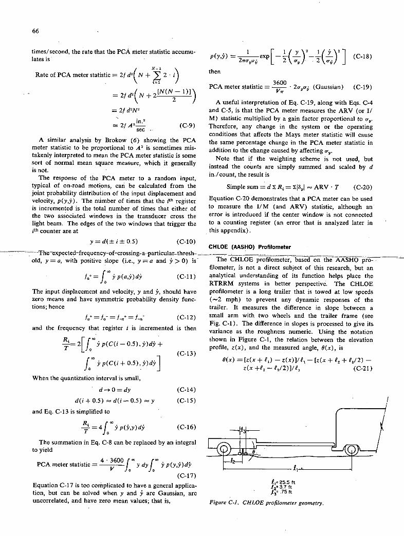
66

times/second, the rate that the PCA meter statistic accumu-latesis

Rate of PCA meter statistic = 2/ d2(N + 2

2/ d2(N + 2 1)])

= 2/ d2N2

2/ A 2 inL (C-9) sec

A similar analysis by Brokow (6) showing the PCA meter statistic to be proportional to A2 is sometimes mis-takenly interpreted to mean the PCA meter statistic is some sort of normal mean square measure, which it generally is not.

The response of the PCA meter to a random input, typical of on-road motions, can be calculated from the joint probability distribujion of the input displacement and velocity, p(y,'). The number of times that the jth register is incremented is the total number of times that either of the two associated windows in the transducer cross the light beam. The edges of the two windows that trigger the th counter are at

1 r l

yi

/y\ 1f\1 p(y,') exP

2[—.-(--;j —T(;ç;)

2

] (C-18) 2iw-u-

then

PCA3600

meter statistic = (Gaussian) (C-19) VIT

A useful interpretation of Eq. C-19, along with Eqs. C-4 and C-5, is that the PCA meter measures the ARV (or I! M) statistic multiplied by a gain factor proportional to os,. Therefore, any change in the system or the operating conditions that affects the Mays meter statistic will cause the same percentage change in the PCA meter statistic in addition to the change caused by affecting

Note that if the weighting scheme is not used, but instead the counts are simply summed and scaled by d in./count, the result is

Simple sum = d R= ARV T (C-20)

Equation C-20 demonstrates that a PCA meter can be used to measure the J/M (and ARV) statistic, although an error is introduced if the center window is not connected to a counting register (an error that is analyzed later in this appendix).

y=d(±i±0.5) (C-b) CHLOE (AASHO) Profilometer

old, y = a, with positive slope (i.e., y = a and > 0) is The CHLOE profilometcr, based iihe AASHO filometer, is not a direct subject of this research, but an

p

= J ) p(a,)d' (C-li) analytical understanding of its function helps place the

° RTRRM systems in better perspective. The CHLOE

The input displacement and velocity, y and 5', should have profilometer is a long trailer that is towed at low speeds

zero means and have symmetric probability density func- (-2 mph) to prevent any dynamic responses of the tions; hence trailer. It measures the difference in slope between a

(C-l2) small arm with two wheels and the trailer frame (see Fig. C-i). The difference in slopes is processed to give its

and the frequency that register i is incremented is then variance as the roughness numeric. Using the notation r

f p(C(i —0.5), 5')d5' + shown in Figure C-i, the relation between the elevation

T L o = 21 5' proffle, z(x), and the measured angle, 0(x), is

(C-i 3)

/ 5' p(C(i + 0.5), 5')d5'] 0(x) = [z(x + 1) — z(x)1/81 — [z(x + 12 + 13/2) — z(x +19 - 13/2)1/13 (C-21)

When the quantization interval is small,

d-0=dy (C-i4)

d(i + 0.5) - d(i —0.5) y (C-is)

and Eq. C-13 is simplified to

— = 4 I 5' p(5',y)d5' ((>16) T Jo

The summation in Eq. C-8 can be replaced by an integral to yield

PCA meter statistic =

3600j00 y dyf 5' p(y,$')d5'

(C-17)

Equation C-i 7 is too complicated to have a general applica-tion, but can be solved when y and 5' are Gaussian, are uncorrelated, and have zero mean values; that is,

25.5 ft 1? 3.7 ft /3- .75 ft.

Figure C-i. CHLOE profilometer geometry.

67

where x is the distance traveled from an arbitrary fixed reference point. The slope variance, SV, is then

1 ' SV = 106 . 02 (x)dx (C-22)

ff0

where D is the distance traveled and the 106 factor is traditionally included for convenience in scaling. Equation C-22 is transformed to a complex spatial frequency response function by making the substitutions

z(x) =z()e1 (C-23)

z(x + a) = z(fL)e5) = z(x)e (C-24)

where ( is spatial frequency with units radian/ft and a is an arbitrary distance. The road slope is then

dz(x) =z (x) =jciz(x) (C-25)

dx

The response function between the CHLOE measurement and the actual road slope is found by combining Eqs. C-21 and C-23—C-25 to yield:

H - -

0(2) = ein

-ine,

ei - 1 2eo sin(l'3 /2 z'()

(C-26)

The gain of this response function, JHaJ, is plotted in Figure 8 as a function of wave number (wave number, v/21r = 1/wavelength).

VEHICLE-ROAD CHARACTERISTICS

Vehicle Dynamics

By definition, RTRRM systems measure the response of a host vehicle to road roughness. The different RTRRM systems all involve a measurement of the axle-body motion of the vehicle, and therefore characteristics of the vehicle that affect this motion need to be included in analyses of RTRRM systems. A vehicle ride model can have virtually any conceivable level of complexity—from the minimal, so-called "quarter-car model" with two degrees of freedom (d.o.f.) corresponding to motions of a sprung and unsprung mass—to a complete finite element model with thousands of degrees of freedom, capable of predicting complicated structural resonance characteristics. Discussion in this appendix is limited to the quarter-car model—a limitation justified by the following facts:

Tests conducted with a real passenger car in the laboratory showed little effect of front-axle excitation or rear-axle roll excitation on road meter measurements (see App. D).

A quarter-car simulation, implemented on a GMR profilometer, provided roughness values that correlated as strongly with measurements from in-use RTRRM systems as the systems correlated with each other (see App. B).

Road meter transducers are attached to the axle at a point that is within inches of the roll center (the roll center is a point, determined by suspension kinematics, that does not move relative to the body when the axle is rolled) of virtually all vehicles and theoretically cannot respond to roll movement of that axle.

A 4 d.o.f. model that included front-axle excitation

and body pitch motions was adopted earlier in the research. Predictions from the 4 d.o.f. model concerning changes in measured roughness statistics closely matched those from the 2 d.o.f. model.

The parameters and differential equations that constitute the quarter-car model are shown in Figure 22. The two differential equations are integrated numerically for time-based digital computer studies, or implemented as a similar electronic circuit for analog computer studies. The fre-quency-domain version of the model, namely, the complex response functions, are:

;K1 (K, +JCco) (C-27)

D

= K1(K - u + IC (u)

z D

y - - z8 - K1co2

ZD D

where

K1 = K/M8 ;

K0 = K8 /M8 ;

C = = M,,/M8 ; and

D = pwl - [K1 + K0(1 + ,L)]02 + K1K, + jCoj[K1 +

0 ±/L)w9 (C-30)

In following discussions, the response function of the axle-body motion is designated as H(w) or H(f). The two undamped natural frequencies of this dynamic system are

2 K1 + ( 1 +p)K2 ±V[K j + (1 +i)K2 ] 2 -4aKiK2 2

(C-31)

where the lower natural frequency is usually identified as the body resonance and the higher frequency is the axle resonance. Table C-2 gives the parameter values that define various simulated vehicles, and their response func-tion gains are plotted in Figure B-i and in Figure 7.

Vehicle-Road Interactions

Vehicle ride motions are generally random in nature and thus must be described statistically. The statistical description used for most engineering applications is the spectral density function, which is the partial derivative of the mean-square statistic with respect to frequency. The reason that ride motions are random is, of course, that changes in pavement elevation to which the vehicle re-sponds are random. The basic relationship between spec-tral densities of the input and output of a dynamic system is

G011 (f) = IH(t) 1 2 . G1(f) (C-32)

In the context of this appendix, G0(f) is the spectral density of either axle-body displacement, G0(f), or of axle-body velocity, Gñ(f). Also, G1(f) is either the spectral density of the road elevation, G..(/), or of its vertical velocity, G2(f). (In practice, G00 is usually larger than predicted by Eq. C-32 because of nonlinearities in the system and to other sources of excitation. The equation is

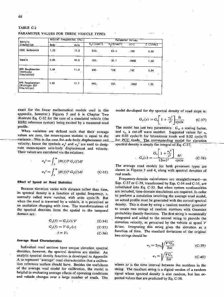
68

TABLE C-2

PARAMETER VALUES FOR THREE VEHICLE TYPES

Natural Frequencies (Hz) Parameter Values __________________________________________ Vehicle

Body Axle K1(l/sec2) K2(l/sec1) u(-) C (1/sec) Simulation

HSRI Reference 1.20 11.0 653. 63.3 .150 6.00

Impala 0.84 10.6 352. 30.1 .0858 1.60

BPR Roughometer 1.64 11.0 640. 128. .162 3.84 (Kentucky Simulation)

BPR Roughometer (Michigan DOT

1.82 17.7 943. 152. .0882 1.05

Simulation)

exact for the linear mathematical models used in this appendix, however.) Figures 5 and 6 in Chapter Two illustrate Eq. C-32 for the case of a simulated vehicle (the HSRI reference system) being excited by a measured road profile.

model developed for the spectral density of road slope is:

G2,(v) = G0[ 1 + _ ft

(C-37) ,2 jcycle

The model has just two ormptprc t c,lin, r--"'" 0 ''""S

When variables are defined such that their average and v0, a cut-off wave number. Suggested values for v0 values are zero, the mean-square statistic is equal to the are 0.05 cycle/ft for bituminous roads and 0.02 cycle/ft

~--~--~variance~T-his=is=the-case~for~axle-body~displacement.arid-----for-F!C~C~-roads. The corresponding model for elevation velocity; hence the symbols 0,2 and are used to desig- spectral density is simply the integral of Eq C-37, nate mean-square axle-body displacement and velocity. r 2 Their values are calculated via the relations: I 1 4.

v2 L IH(f)12 G2(f)df

o.2 = 10 00 111(1)12 G1(f)df

Effect of Speed on Road Statistics

Because elevation varies with distance rather than time, its spectral density is a function of spatial frequency, v, normally called wave number, with units cycle/ft. But when the road is traversed by a vehicle, it is perceived as an excitation changing with time. The transformations of the spectral densities from the spatial to the temporal domain are:

G2(f) = G(v)/V (C-34)

G(/) = V G...(v) (C-35)

f=Vv (C-36)

Average Road Characteristics

Individual road sections have unique elevation spectral densities; however

'the spectral densities are similar. An

analytic spectral density function is developed in Appendix A to represent "average" road characteristics that a calibra-tion reference surface should have. Besides the usefulness of the average road model for calibration, the model is helpful in evaluating average effects of operating conditions and vehicle changes over a large number of roads. The

_°L v2J ft3 - (2irv)2 cyc-;;j (C-38)

The average road models for both pavement types are shown in Figures.3 and 4, along with spectral densities of real roads.

Frequency-domain calculations are straightforward—as Eqs. C-37 or C-38, transformed by Eqs. C-34 and C-35, are substituted into Eq. C-33. But when system nonlinearities are included, time-domain simulations are required. In order to perform a simulation involving the average road model, an actual profile must be generated with the correct spectral density. This is done by using a random number generator to create two strings of random numbers with Gaussian probability density functions. The first string is numerically integrated and added to the second string to provide the elevation velocity, as perceived by the vehicle at speed V ft/sec. Integrating this string gives the elevation as a function of time. The standard deviations of the original two strings should be

O1 2?TVoV__ .

(C-40)

where it is the time interval between the numbers in the string. The resultant string is a digital version of a random signal whose spectral density is also random, but has ex-pected values that are predicted by Eq. C-38.

69

CORRELATION

Measurements made with different instruments can be correlated for two reasons; namely: (1) both instruments measure the same physical quality, although the measure-ment includes a random error due to the limited precision of the instruments; and (2) the instruments measure differ-ent physical qualities, but the two qualities are correlated over a range of measurements.

A simple example of the second reason is the strong correlation between automobile measurements taken with a scale (vehicle weight) and measurements taken with a yardstick (wheelbase). Although the two instruments used have little in common, it is a fact that longer automobiles tend to weigh more, and therefore the measurements are correlated. Similarly, various road roughness measuring systems measure different physical qualities, and correla-tion between the different roughness statistics is largely due to correlation between the different qualities that are measured.

Appendix A describes the similarities between spectral densities of different roads, and then uses them to develop the average road models described by Eqs. C-37 and C-38. Such models have validity only because road roughness levels at different wave numbers are correlated. That is, a road with high roughness content in the low wave number range is likely to have high roughness content in the high wave number range. The practical result of this tendency is that virtually any instrument that produces a measure-ment in some way related to road roughness will correlate to some extent with other systems.

Although roads have spectral densities similar to the model, the spectral density of any particular length of pave-ment is still unique. A characteristic of spectral densities is that the variance of a measured spectral density function at one frequency is large, but when the function is averaged over a frequency interval, the variance decreases according to the relation:

G

_ 2 (f)

Variance - (C-41) BT

where B is the frequency bandwidth (30). (This is only valid for broadband type variables—a category that in-cludes the elevation and slope of most roads.) This characteristic can be observed in the measured spectral densities shown in Figures 3 and 4 and in Figures A-5 and A-6. Although the curves have underlying shapes over the entire wave number range, they vary tremendously over limited wave number intervals. (The figures do not show this completely, because some frequency averaging had been done prior to the plotting of the functions to reduce the visible "hash" in the curves.) The practical effect of this characteristic is that measurements deriving from a narrow band of wave numbers are more subject to these variances and will correlate more poorly with mea-surements from different systems than will measurements deriving from a broader band of wave numbers.

COMPARISON OF DIFFERENT ROAD ROUGHNESS

MEASUREMENT SYSTEMS

Having presented mathematical models of the different

road meters, the CHLOE, and the vehicle, the question, "What quantity is measured by different road roughness measuring ,systems?" can be addressed. Table C-3 gives the responses of the various systems to sinusoidal excita-tion and to random, stationary, Gaussian excitation. As previously noted, perfect correlation cannot be expected between the different systems because a deterministic relationship does not exist. Nevertheless, when the average road model (Eqs. C-34—C-38) is used in place of the road spectral densities in the table, the underlying relationships between the different roughness statistics are evident. The Mays meter and BPR roughometer systems then produce statistics proportional to 'VG0, while all the other statistics are proportional to G0. Thus, over a large number of roads, linear trends should relate the PCA meter, CHLOE, and Michigan DOT statistics, which should all then be related 'to the Mays meter and BPR roughometer statistics by a quadratic trend.

Frequency Content of Roughness Statistics

The frequency content of a mean-square statistic is seen from the spectral density, but the frequency distribution curve, defined as

[ F(f)

= Jo (C-42)

1,0 G()d is a more convenient function for presenting the frequency content of a mean-square statistic, because the portion of the overall statistic deriving from the frequency range, f :!~ / :!~ /2 is simply F(f 2) - F(f 1) percent.

Figure C-2 shows frequency distribution curves for the case of the HSRI-reference system subject to excitation from the average bituminous road model when traversed at 50 mph. Note that about 93 percent of the mean-square axle-body displacement, o,2, derives from frequencies less than 2.0 Hz, whereas only 35 percent of the mean-square axle-body velocity, 02, is contained in this range (o,2 is seen to be fairly well spread out over the frequency range of 1-15 Hz). Under the ideal conditions of a stationary and Gaussian road, linear vehicle, and perfect road meter, the Mays meter statistic is proportional to (ri and the PCA meter statistic is proportional to Figure C-2 can thus be interpreted to show the frequency distribution of the square of the Mays meter statistic and the frequency distri-bution of the two factors of the squared PCA meter statis-tic. Although a precise description of the direct frequency content of the roughness statistic is not possible, it is clear that the Mays meter statistic is sensitive to vibrations in the frequency range of 1-15 Hz, whereas the PCA meter statistic—which is also dependent on the vibrations in the same 1-15-Hz range—at the same time is much more sensitive to the vibrations in the 0-2-Hz range.

Although RTRRM systems do, by definition, measure the dynamic response of the 'host vehicle, system users are really concerned with the physical features of the road. Figure C-3 shows frequency distribution curves for various

-- /

/ /

/ Axle-Body Displacement

Axle-Body Velocity

/ I I I I

I I I I I I I I I

70

TABLE C-3

COMPARISON OF IDEAL ROAD ROUGHNESS MEASUREMENT SYSTEMS

Sine Wave Response A = amplitude Response To

System Type Units Roughness Numeric f,v = frequency* Gaussian Excitation

1/2 Mays meter Response in/mi average rectified 4fAIH(f)I 1

11J IH(f)I 20.(f)df] and BPR velocity of axle- V V [ii roughometer body motion, di-

vided by vehicle j speed =

PCA meter Response in/mi 2 PCA meter statistic 2fA2 IH(f)I 2

1f H(f)I2G(f)df V

1/2

f H(f)t2G(f)df] Vii

CHLOE Absolute slope2 frequency weighted IHc(v)12A2(211v)2 (AASHO) x 106 slope variance 106 = SV Profilo- meter

Michigan Absolute in2 frequency weighted A2 < < .02 DOT Pro- elevation variance 2 ' - - G (v)dv EV filometer (see Ch. 0 otherwise 02

2in report)

*f is temporal frequency, in Hz, while v is spatial frequency, in cycle/ft. Note: In this table, speed (v) has the units mile/sec.

100 -- ___— --,s— -

::

80

CLOESV — — — MOOT EV

60

40 II I y/

20

I

0 I i I I 1111. 0.O0 4.00 8.00 12.00 16.00 20.00 24.00 .001 Wave Number (cycle/ft)

FrequenCy (Hz)

Figure C-2. Frequency distribution curves for axle-body dis- Figure C-3. Wave number content of various road roughness placement and velocity for the reference system traversing an statistics. average bituminous road at 50 mph.

mean-square roughness statistics as functions of wave RTRRM system is 50 mph (73.7 ft/sec); thus the fre- number vf/V cycle/ft. Using the figure as a reference, quency range 1-15 Hz that contains most of the o the frequency-wave number content of the various statistics statistic corresponds to the wave number range 0.014— can be discussed. 0.205 cycle/ft.

Mays Meter PCA Meter

Normal measurement speed for a Mays-meter-based One component of the squared PCA meter statistic is

71

which has the same wave number content as the square of the Mays meter statistic. The second component,

is seen to derive mostly from the wave number range 0.005-0.025 cycle/ft. Because this range accounts for only 30 percent of the correlation between PCA meter statistic and Mays meter statistic is limited by the correla-tion in the roughness levels of the different wave number ranges.

BPR Roughometer

BPR roughometer trailers have dynamic characteristics that may or may not resemble those of passenger cars, as shown in Figure 7. But an unavoidable difference is that BPR roughometers are operated at 20 mph instead of the nominal 50-mph speed associated with Mays- and PCA-meter-based systems. The result is that a BPR roughometer is excited by a different portion of the road roughness, deriving from higher wave numbers (see Eq. C-36 for the transformation). Figure C-3 shows that the Kentucky BPR roughometer simulation is virtually unaffected by roughness distributed over wave numbers less than 0.05 cycle/ft, even though nearly half of 02 for the HSRI-reference system is due to this portion of the road rough-ness. The reference system does not respond to roughness distributed over wave numbers greater than 0.25 cycle/ft; yet, over half of the response of the BPR roughometer derives from that range. Clearly, the correlation between a BPR roughometer and a Mays meter system is com-promised because the overlap in the wave number range that affects each system accounts for only half of each (squared) measurement. Note that virtually no overlap exists between the wave number ranges that excite BPR roughometer o.,2 and HSRI-reference system o- 2--thereby implying that BPR roughometer and PCA meter measure-ments should not correlate as well as BPR roughometer and Mays meter measurements.

CHLOE Pro filometer

The CHLOE slope variance, SV, is influenced by rough-ness distributed even beyond the wave number range 0.001-1 cycle/ft shown in the figure. The best match with the CHLOE appears to be the HSRI-reference which is a response to roughness in the wave number range of 0.05-0.5 cycle/ft—a range that accounts for about 50 percent of SV. The total range of the BPR roughometer

2 accounts for 45 percent of SV, and the portion of overall roughness that causes the response accounts for about 20 percent of SV.

Michigan DOT

The weighted elevation variance, EV, described in the report, is intentionally limited to the wave number range 0.02-0.5 cycle/ft. Because it is a mean-square measure of elevation, it mostly reflects the high-amplitude, low-wave number portion of that range. The EV is seen to measure a portion of the overall roughness that just barely overlaps the portions that contribute to the squared BPR roughometer measurement and the HSRI-reference

The 0.02-0.07 cycle/ft range, which contains 90 percent of the EV, contributes about 33 percent of the HSRI reference and about 15 percent of the CHLOE SV.

EFFECTS OF VARIABLES ON RTRRM SYSTEM PERFORMANCE

Operating Speed

Operating speed has been shown to affect roughness statistics from RTRRM systems in two ways. First, the current practice of normalizing the road meter output by the length of the test section introduces a speed effect, evidenced by the 1/V scaling factor in the mathematical descriptions of the statistics (see Eqs. C-4 and C-8, and Table C-3). This effect is eliminated by normalizing the meter outputs to the time duration of the test—a practice recommended in the report for a variety of reasons. When the Mays meter measurement is normalized by time, the resultant statistic is simply the ARV of the axle-body motion. The PCA meter statistic remains complicated no matter how it is normalized. The remainder of this appen-dix discusses the rate of the statistics, designated ARV and PCA rate, to exclude this first speed effect.

The second speed effect is the changing perception of the road (as a time varying input) with speed, an effect specified by Eqs. C-34—C-36 and discussed to some extent in the comparison of the BPR roughometer to the Mays meter system. Figure C-4 shows the speed sensitivities of the ARV and PCA rate statistics, based on the HSRI-reference simulation, by using Eqs. C-33--C-38 and the Gaussian input assumption. The speed sensitivity results partially from the high roughness content in the low wave number region, with the result that speed effects are greater for bituminous roads than for PCC roads, and are greater for the PCA rate than the ARV.

ARV (a;) on PCC Road

ARV (a;) on Bituminous Road

PCA-Rate (oyop) on PCC Road

PCA-Rate (no.) on Bituminous Road

10 20 30 40 50 60 70

Speed (mph)

Figure C-4. Speed eflect on ARV and PCA meter rate.

200

C

100

r

72

Vehicle Parameters

The simple quarter-car model shown in Figure 22 was proved to be a reasonable predictor of the dynamic re-sponse of real passenger cars, as they affect RTRRM-system performance. A good understanding of the quarter-car model is a solid step towards understanding the behavior of real vehicles. The model is defined by just four parameter values, which have been normalized by the sprung mass value; but, because the sprung mass is a variable of interest, it is also considered here.

Figure C-S shows the effect that changes in each parame-ter have on the vehicle response function, by showing the response functions for both an increase of 25 percent and a decrease of 25 percent of each parameter from its base-line value given in Table C-2. Changes that increase the gain of the response function will act to increase the roughness statistics. Changes that. broaden the band of frequencies contributing to the mean-square statistic will also act to increase the measurements. Because axle-body velocity has contributions over the frequency range 1-15 Hz (see Fig. C-2), oj,2—and hence ARV—will be affected by any changes in the response function within this range. But the axle-body displacement just has frequency content from 0-2 Hz, so 0 2—ánd hence o-,a- and PCA rate—are more sensitive to changes involving the body resonance.

Combining the changes in response function with the road • gives the changes to u-11 and o- . Figure C-6 shows the sensitivities of .o (ARV) and (PCA rate) for two vehicle types; namely, the HSRI-reference and the Impala (see Table C-2 and Fig. B-i), responding to rough-ness from the average bituminous road model. The figures are fairly self-explanatory, so the trends are just briefly summarized in the following.

Damping Rate

The damper, C8, is seen to affect the roughness statistics more than any of the other vehicle parameters. Increasing C8 acts to move the body- and axle-resonance frequencies in towards each other, away from the undamped natural frequencies defined by Eq. C-3 1. More importantly, increasing C8 reduces the gain at the two peaks, thereby flattening the response function curve. As a result, the roughness statistics are decreased, and the frequency con-tent of the squared statistics is not as sensitive to the road roughness contained in the narrow wave number bands near the two resonances. Based on the earlier discussion, correlation between measurements of the different RTRRM systems would be expected to improve when the C. value for one or both of the systems is increased.

An interesting aspect of the response sensitivity to C. is

Vary Mu

Vary K5

0 10 20

10

I0

0

Vary K

Th'0 26 0 10 20

Frequency (Hz)

+25% Baseline Value

-25% Baseline Value

72

/\

, U / rVaryCs

0010

Frequency (Hz)

Figure C-5. Effect of parameter variation on the reference vehicle re-sponse function.

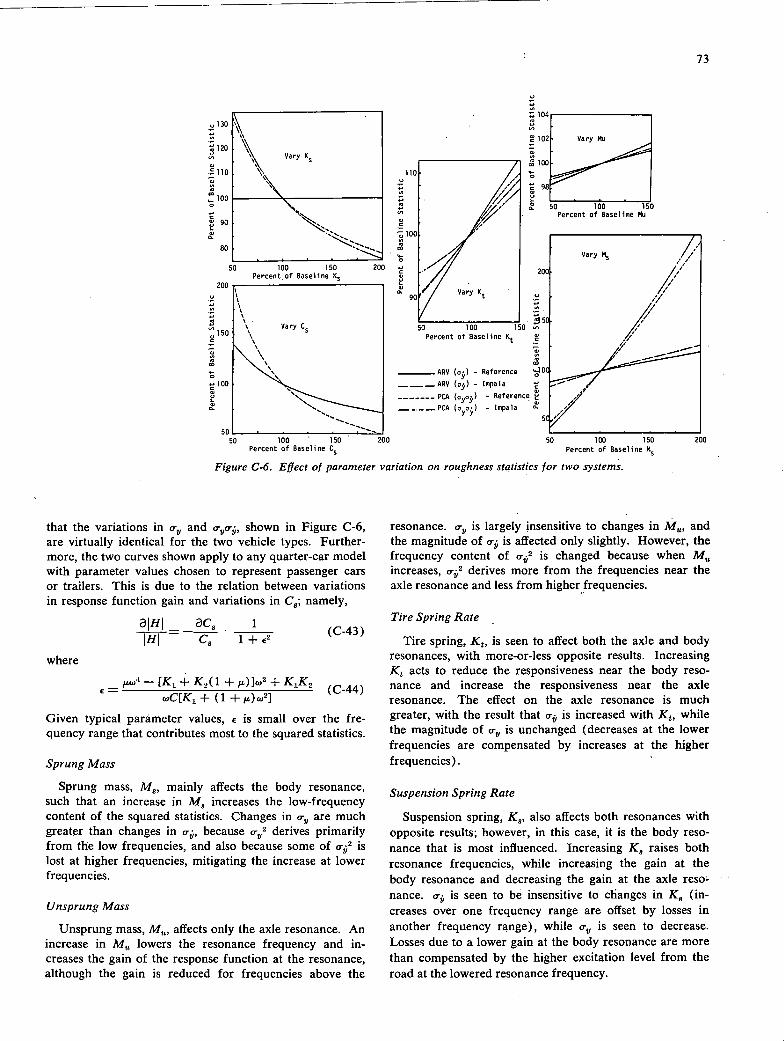
Vary KS

100 150 200 Percent of Baseline K5

Vary C. 7

50 L 50

100 150 200 Percent of Baseline C5

73

10

102 Vary Ma

100

110

98

50 100 150 Percent of Baseline Mu

100

Vary M5 /

200

90

-15

/ Percent of Baseline Kt .

ARV (o;) - Reference

___ARV (op) - impala 1.

PCA (nyu;) - Reference ul

__...._PCA (no;) - impala .

50 100 150 200 Percent of Baseline Ms

130

120

. 110

100

90

80

50

200

150

.-. 100

Figure C-6. Eftect of parameter variation on roughness statistics for two systems.

that the variations in cry and shown in Figure C-6, are virtually identical for the two vehicle types. Further-more, the two curves shown apply to any quarter-car model with parameter values chosen to represent passenger cars or trailers. This is due to the relation between variations in response function gain and variations in Ca; namely,

aIHI aCa . i'r c8

where

- [K1 + K2(1 + LL)])2 + K1K2

coC[K1+ (1 +,$)caZ]

Given typical parameter values, € is small over the fre-quency range that contributes most to the squared statistics.

Sprung Mass

Sprung mass, M3, mainly affects the body resonance, such that an increase in M3 increases the low-frequency content of the squared statistics. Changes in a-8 are much greater than changes in because 09,2 derives primarily from the low frequencies, and also because some of 02 is lost at higher frequencies, mitigating the increase at lower frequencies.

Unsprung Mass

Unsprung mass, M,4, affects only the axle resonance. An increase in M55 lowers the resonance frequency and in-creases the gain of the response function at the resonance, although the gain is reduced for frequencies above the

resonance. cr, is largely insensitive to changes in M, and the magnitude of o- is affected only slightly. However, the frequency content of is changed because when M increases, derives more from the frequencies near the axle resonance and less from higher frequencies.

Tire Spring Rate

Tire spring, K, is seen to affect both the axle and body resonances, with more-or-less opposite results. Increasing Kt acts to reduce the responsiveness near the body reso-nance and increase the responsiveness near the axle resonance. The effect on the axle resonance is much greater, with the result that crj is increased with K, while the magnitude of o- , is unchanged (decreases at the lower frequencies are compensated by increases at the higher frequencies).

Suspension Spring Rate

Suspension spring, Ka, also affects both resonances with opposite results; however, in this case, it is the body reso-nance that is most influenced. Increasing K3 raises both resonance frequencies, while increasing the gain at the body resonance and decreasing the gain at the axle reso- nance. is seen to be insensitive to changes in Ka (in- creases over one frequency range are offset by losses in another frequency range), while a-8 is seen to decrease. Losses due to a lower gain at the body resonance are more than compensated by the higher excitation level from the road at the lowered resonance frequency.

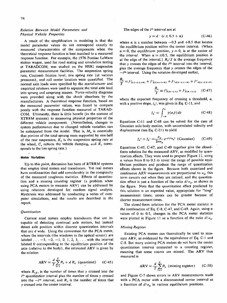
74

Relation Between Model Parameters and Physical Vehicle Properties

A result of the simplification in modeling is that the model parameter values do not correspond exactly to measured characteristics of the components when the theoretical response function is best matched to a measured response function. For example, the 1976 Pontiac LeMans station wagon, used for road testing and simulation testing at TARADCOM, was studied on the HSRI suspension parameter measurement facilities. The suspension spring rate, Coulomb friction level, tire spring rate (at various pressures), and roll center location were quantified. The normal axle loads were specified by the manufacturer and empirical relations were used to separate the total axle load into sprung and unsprung masses. Force-velocity diagrams were provided along with the shock absorbers by the manufacturers. A theoretical response function, based on the measured parameter values, was found to compare poorly with the response function measured at TARAD-COM. Ultimately, there is little benefit (in the context of RTRRM systems) to measuring physical properties of the different vehicle components. (Nevertheless, changes in system performance due to changed vehicle variables can be anticipated from the model. That is, M8 is essentially that portion of the total sprung mass supported by one-half of the rear suspension, K8 is the suspension spring rate at the wheel, C8 reflects the vehicle darripitig, and Kt corrc-sponds to the tire spring rate.)

Meter Variables

Up to this point, discussion has been of RTRRM systems that employ ideal meters and transducers. Yet real meters have nonlinearities that add considerably to the complexity of the measured roughness statistics. Effects of quantiza-tion and a missing counting register (a problem when using PCA meters to measure ARV) can be addressed by using relations developed for random signal analysis. Hysteresis was addressed by conducting a series of com-puter simulations, and the results are described in the report.

Quantization

Current road meters employ transducers that are in-capable of detecting continual axle motion, but instead detect axle position within discrete quantization intervals that are d wide. Using the convention for the PCA meter, where the intervals (the windows in the optical sensor) are labeled . . . —3, —2, —I, 0, 1, 2, 3, . . . with the interval labeled 0 corresponding to the equilibrium position of the axle (relative to the body), the estimated ARV is given by the relation

ARV = 4-R + d R0 (quantized) (C-45)

where Ri p is the number of times that y crossed into the ith quantization interval plus the number of times y crossed into the _ith interval, and R0 is the number of times that y crossed into the center interval.

The edges of the jth interval are at

y = d (i ± 0.5 + a) (C-46)

where a is a number between —0.5 and +0.5 that locates the equilibrium position within the center interval. (When a = 0, the equilibrium position, y = 0, is at the center of the interval. When a = ±0.5, the equilibrium position is at the edge of the interval.) R/ T is the average frequency that y crosses the edges of the jtli interval into the interval, plus the average frequency that y crosses the edges of the _ith interval. Using the notation developed earlier,

— f1(i-0.5+a) + I (+oF+a) + I-d(i-0.5-) + ttd(+0.5-a)

= Ia-o. + Id(+0.5) (C-47)

where the expected frequency of crossing a threshold, a, with a positive slope, /, was given in Eq. C-il, and

Ia f (a,) d? (C-48) J -

Equations C-il and C-48 can be solved for the case of Gaussian axle-body motion, with uncorrelated velocity and displacement (see Eq. C-21) to yield

- fa -' e'212°i (Gaussian) (C-49) - Equations C-45, C-47, and C-49 together give the closed-form solution for the measured ARV, as modified by quan-tization effects. They were used to prepare Figure 11, using a values from 0 to 0.5 to cover the range of possible equi-librium positions and produce the range of quantization effects shown in the figure. Because both quantized and continuous ARV measurements are proportional to o, this term cancels out when they are ratioed, and the quantiza-tion effect is just a function of the ratio d/cr, as shown in the figure. Note that the quantization effect predicted by this solution is an expected value, appropriate for "long" measurement times; errors can be greater because of shorter measurement times.

The closed-form solution for the PCA meter statistic is the combination of Eq. C-8, C-47, and C-49. Again, using a

values of 0 to 0.5, changes in the PCA meter statistics were plotted in Figure 11 as a function of the ratio dl o.

Missing Register

Existing PCA meters can theoretically be used to mea-sure ARV, as evidenced by the equivalence of Eq. C-I and C-8. But many existing PCA meters do not have the center quantization interval connected to a counting register, meaning that some counts are missed. The ARV thus measured is

ARV =.4_R (missing register) (C-SO)

and Figure C-7 shows errors in ARV measurements made with a PCA meter with a disconnected center interval as a function of d/o- in various equilibrium positions.

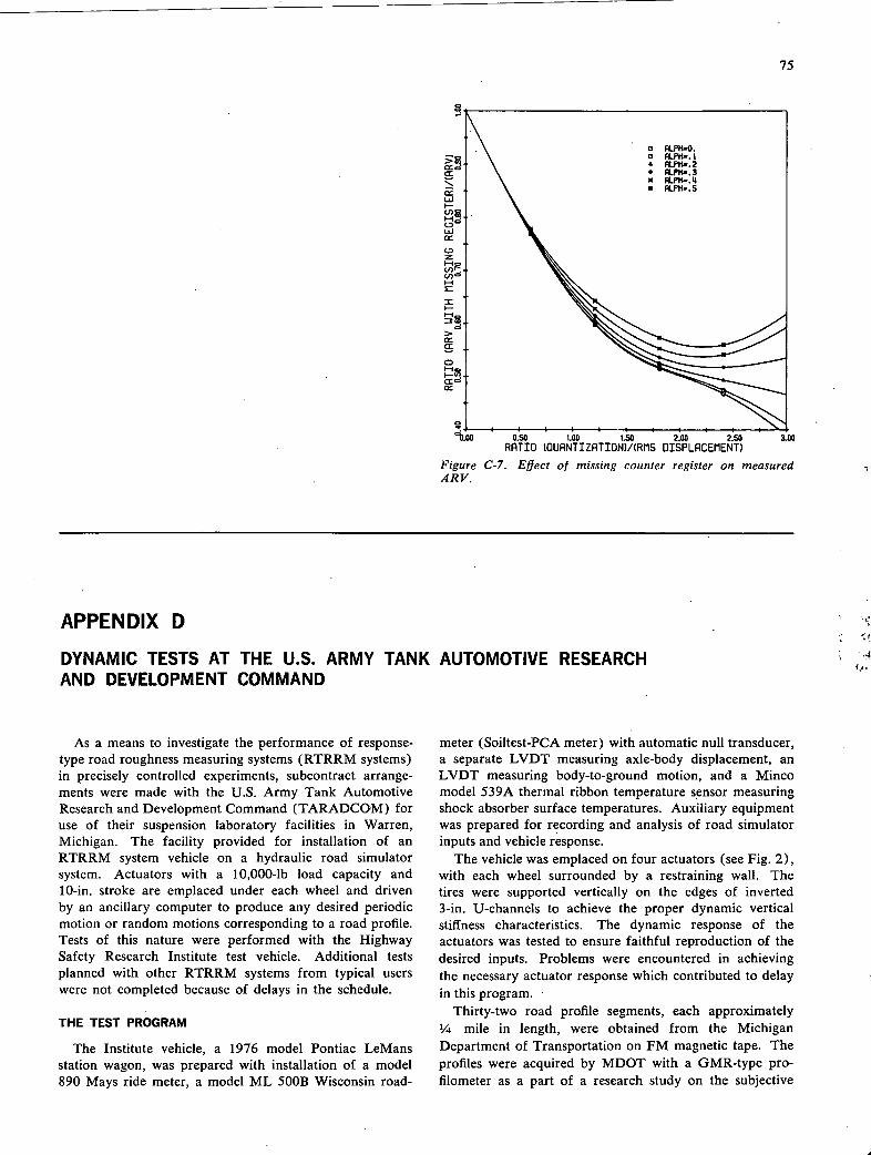
75

RATIO (OIJANTIZATION)/(RrIS DISPLACEMENT)

Figure C-7. Eflect of missing counter register on measured ARV.

DYNAMIC TESTS AT THE U.S. ARMY TANK AUTOMOTIVE RESEARCH AND DEVELOPMENT COMMAND

As a means to investigate the performance of response-type road roughness measuring systems (RTRRM systems) in precisely controlled experiments, subcontract arrange-ments were made with the U.S. Army Tank Automotive Research and Development Command (TARADCOM) for use of their suspension laboratory facilities in Warren, Michigan. The facility provided for installation of an RTRRM system vehicle on a hydraulic road simulator system. Actuators with a 10,000-lb load capacity and 10-in, stroke are emplaced under each wheel and driven by an ancillary computer to produce any desired periodic motion or random motions corresponding to a road profile. Tests of this nature were performed with the Highway Safety Research Institute test vehicle. Additional tests planned with other RTRRM systems from typical users were not completed because of delays in the schedule.

THE TEST PROGRAM

The Institute vehicle, a 1976 model Pontiac LeMans station wagon, was prepared with installation of a model 890 Mays ride meter, a model ML 500B Wisconsin road-

meter (Soiltest-PCA meter) with automatic null transducer, a separate LVDT measuring axle-body displacement, an LVDT measuring body-to-ground motion, and a Minco model 539A thermal ribbon temperature sensor measuring shock absorber surface temperatures. Auxiliary equipment was prepared for recording and analysis of road simulator inputs and vehicle response.

The vehicle was emplaced on four actuators (see Fig. 2), with each wheel surrounded by a restraining wall. The tires were supported vertically on the edges of inverted 3-in. U-channels to achieve the proper dynamic vertical stiffness characteristics. The dynamic response of the actuators was tested to ensure faithful reproduction of the desired inputs. Problems were encountered in achieving the necessary actuator response which contributed to delay in this program.

Thirty-two road profile segments, each approximately ¼ mile in length, were obtained from the Michigan Department of Transportation on FM magnetic tape. The profiles were acquired by MDOT with a GMR-type pro-filometer as a part of a research study on the subjective

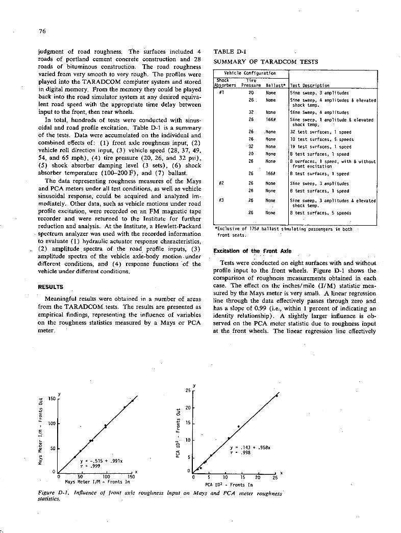
V

150 0

4-, S 0 I-

100

a) 50

(0

0

y 25

. 20 0

15 0 I. 'S.

10 0

C, 0 5

0 x

76

judgment of road roughness. The surfaces included 4 roads of portland cement concrete construction and 28 roads of bituminous constructiOn. The road roughness varied from very smooth to very rough. The profiles were played into the TARADCOM computer system and stored in digital memory. From the memory they could be played back into the road simulator system at any desired equiva-lent road speed with the appropriate time delay between input to the front, then rear wheels;

In total, hundreds of tests were conducted with sinus-oidal and road profile excitation. Table D-1 is a summary of the tests. Data were accumulated on the individual and combined effects of: (1) front axle roughness input, (2) vehicle roll direction input, (3) vehicle speed (28, 37, 49, 54, and 65 mph), (4) tire pressure (20, 26, and 32 psi), (5) shock absorber damping level (3 sets), (6) shock absorber temperature (100-200 F), and (7) ballast.

The data representing roughness measures of the Mays and PCA meters under all test conditions, as well as vehicle sinusoidal response, could be acquired and analyzed im-mediately. Other data, such as vehicle motions under road profile excitation, were recorded on an FM magnetic tape recorder and were returned to the Institute for further reduction and analysis. At the Institute, a Hewlett-Packard spectrum analyzer was used with the recorded information to evaluate (1) hydraulic actuator response characteristics, (2) amplitude, spectra of the road profile inputs, (3) amplitude spectra of the vehicle axle-body motion under different conditions, and (4) response functions 'of the vehicle under different conditions.

RESULTS

Meaningful results were obtained in a number of areas from the TARADCOM tests. The results are presented as empirical findings, representing the influence of variables on the roughness statistics measured by a Mays or PCA meter.

TABLE D-1

SUMMARY OF TARADCOM TESTS

Vehicle Configuration

Shock Tire Absorbers Pressure Ballast* Test Description

#1 20 None Sine sweep, 3 amplitudes

26 , None Sine sweep, 4 amplitudes & elevated shock temp.

32 None Sine Sweep, 4 amplitudes

26 166# Sine sweep, 1 amplitude & elevated shock temp.

26 None 32 test surfaces, 1 speed

26 None 10 test surfaces, 5. speeds

'32 None 19 test surfaces, 1 speed

20 None 8 test surfaces, 1 speed

26 None 8 surfaces, 1 speed, with & without front excitation

26 166# 8 test surfaces, 1 speed

#2 26 None Sine sweep, 3 amplitudes

26 None 8 test surfaces, 1 speed

#3 26 None Sine sweep, 3 amplitudes & elevated shock temp.

26 None 8 test surfaces, 5 speeds

*Exclusive of 175# ballast simulating passengers in both

front seats.

Excitation of the Front Axle

Tests were conducted on eight surfaces with and without profile input to the front wheels. Figure D-1 shows the comparison of roughness measurements obtained in each case. The effect on the inches/mile (I/M) statistic mea-sured by the Mays meter is very small. A linear regression line through the data effectively passes'through zero and has a slope of 0.99 (i.e., within 1 percent of indicating an identity relationship). A slightly larger influence is ob-served on the PCA meter statistic due to roughness input at the front wheels. The linear regression line effectively

Mays Meter JIM - Fronts In DrA 2 r..,....... ,.

Figure D-1. Influence of front axle roughness input on Mays and PCA meter roughness statistics.

77

passes through zero and has a 0.96 slope (i.e., within 4 percent of an identity relationship). These results are in agreement with the observations made in sinusoidal testing —namely, that front-axle excitation produced negligible response of the rear axle-body displaccmcnt. It is felt that these findings provide the basis for discounting the need for calibrating the front suspension of a vehicle used for roughness measurements. Hence, the only attention needed on the front suspension of such vehicles is normal main-tenance as required to ensure proper wheel balance, align- ment, etc. -

Tire Pressure

Rear tire inflation pressure has a significant effect on vehicle response and roughness measurement. This conclu-sion is drawn from sinusoidal response tests and tests in which the vehicle was "operated" with different inflation pressures over the same set of eight road profiles. Pressure in the vehicle's HR 78-15 steel-belted radial tires was varied from the normal value of 26 psi, to 20 psi, and to 32 psi. Figure D-2 shows the effect of rear tire pressure changes on the vehicle's sinusoidal response. The tire pressure has its strongest effect on rear axle resonance by its influence on the effective stiffness of the tire. Figure D-3 shows the trend of effects on the JIM statistic gen-erated by the Mays meter and the PCA meter statistic. For the JIM statistic, the relationship is well represented by linear regression lines that pass through the origin and indicate a slope or gain factor equivalent to +4 percent! 6 psi increase in tire pressure. Correlation coefficients greater than 0.99 are obtained.

The PCA meter statistic shows a comparable influence of tire pressure, although the effect is about twice as large.

.2 2

Jo 20 Frequency (Hz)

Figure D-2. Effect of tire pressure on vehicle response.

Specifically, a 7 percent increase in the statistic occurs with a 6-psi increase (26 to 32 psi) in pressure, and a 9 percent decrease with a 6-psi decrease (26 to 20 psi) in pressure.

y y A 25 /

/

20 32PS1. / /

CD 150 32 PSI / y = -.14 + 1 07x /

y=-.31+i.04x / r = .999

r = .999

: '::PSIo

20 PSIo

50f +96x

y = .20 + .91x a- 5 r=.998

r::996

•

x 0 50 100 150 0 5 10 15 20 25

Mays Meter I/M (26 psi) PCA Meter ED2 (26 psi)

Figure D-3. influence of rear-axle tire pressure on Mays and PCA meter roughness statistics.

V 50 100 150 200 Mays Meter !/M - Unballasted

0 5 10 15 20 25 30

PCA 02 - Unballasted

200 35

30

10

78

Ballast

The sprung mass of a vehicle is a variable of concern because of the differences associated with vehicle type and the miscellaneous load carried on-board. TARADCOM tests were designed to quantify the influence of vehicle - Ballasted Vehicle

mass on roughness measurement. When set up in the S Unballasted Vehicle

facility, the test vehicle was ballasted with 175 lb of sand- -

bags in each front seat, simulating the driver and a pas-senger. In subsequent testing, steel ballast totaling 166 lb (equivalent to 20 gal of fuel and a 36-lb suitcase) were placed in the trunk of the vehicle, and sinusbidal tests were conducted along with runs on eight road surfaces.

Figure D-4 shows the effect of ballast load on the vehicle response. The dominant effect is the reduction of the body

1 -

bounce frequency and a reduction of damping ratio. \ Figure D-5 shows the influence of ballast on Mays and I

PCA meter roughness statistics. The influence on both I

1 statistics is represented by the slope of the linear regression lines, which is the effective sensitivity or gain. The J/M

I

statistic proves to be least influenced by ballast, a result 00 I 10

I

that supports the analytical findings in Appendix C. The " Frequency (liz) 20

plotted data indicate a 4 percent increase in I/M with the Figure D-4. Eftect of ballast on vehicle response. 166 lb of - ballast.

The influence of ballast on the PCA meter statistics, as expected from the analysis in Appendix C, is much

levels of damping. Comparative tests were performed at stronger. The data show a 41 percent increase with the TARADCOM to measure the influence of these shock absorbers- on~thc~roughnessstatistics=generated-by the-Mays variable with PCA meter systems. and PCA meters. In total, three sets of shock absorbers

Shock Absorber Damping Level were tested:

Perhaps the most influential and difficult variable to be controlled is the damping within the suspension. Earlier tests on the Institute vehicle established that shock absorb-ers were clearly the dominant source of damping on the rear suspension. Through the cooperation of the Monroe Auto Equipment Company, two pretested' sets of shock absorbers were obtained to represent typical high and low

Set #1—Monroe-Matics (Part No. 3082) Set #2—Delco Big D (Part No. 22002586) Set #3—Monroe Grabbers (Part No. 1351177)

The shock absorbers, through their damping, affect vehicle response directly. Figure D-6 contrasts the response changes with shock absorber sets #1 and #3. The effect on roughness measurement is as shown in Figure D-7.

Figure D-5. Influence of vehicle sprung mass (ballast) on Mays and PCA meter roughness statistics.

Set 1

Set 3

PJ

8 12 16 20 24 rrequency (Hz)

Figure D-6. Effect of different shock absorbers on measured vehicle response junction.

The relationship for the JIM statistic is characterized by a 30 percent difference in slope, plus an offset that is more significant than was observed with other variables. The offset is the result of meter hysteresis. With a decrease in damping, the greater vehicle response diminishes the mea-surement losses due to hysteresis, creating the offset shown. The PCA meter statistic is influenced even more, with this statistic changing by a factor of two.

Less directly, the operating temperature affects shock absorber damping. No provisions were made for con-

79

trolling shock absorber temperature to assess the effect at TARADCOM. Nevertheless, elevated temperatures could be achieved in the sinusoidal response tests. Figure D-8 shows the change in response function when the shock absorbers were allowed to heat up to approximately 200 F. Because the strongest influence occurs at body resonance, temperature would be expected to have a greater effect on the PCA meter statistic.

The nonlinerity of shock absorber damping effects became quite evident in the TARADCOM tests. Response measures at different tire input amplitudes strongly affected the relative response obtained. Figure 18 in Chapter Two shows measured response at different input amplitude compared to the equivalent response with road profile inputs. The comparison vividly shows that true and valid measures of vehicle response are only obtained with sinusoidal inputs at appropriate excitation amplitudes.

Speed

Characterizing the effects of test speed was an issue vital to the research project. The TARADCOM tests provided the opportunity to examine the influence of speed on the roughness statistic obtained, in the absence of vehicle specific effects such as tire and driveline imbalance, aero-dynamic disturbances, etc.

Uiider these ofltf011ed conditions, speed variations produced diverse changes in the roughness statistic ob-tained, reflecting different vehicle tuning to the wavelength content of each road at each speed. Figure D-9 shows the effect of speed observed on eight different surfaces. The IIM statistic is shown rather than the ARV statistic dis-cussed in the main report. The effect of speed on the JIM, as shown, derives from two mechanisms—increasing ARV and decreasing travel time. These tend 'to cancel, resulting in less apparent speed sensitivity to the JIM than the ARV statistic. These data show that the influence of test speed is specific to each surface, as well as to the statistic being

200

0

0 150

I- 100

0)

>

50

60

50

0,

4-) o 40

U 0

30

a

20 0

10

Mays Meter I/M - Shock Set #1

PCA tD - Shock Set #1

Figure D-7. Influence of typical rear-axle shock absorbers on the measured Mays and PCA meter roughness statistics.

80

Roll inputs-are not expected to produce significant influ- ' cncc on roughness measurement because the transducers

are normally attached near the roll center of the vehicle , suspension. Roll response was measured by sinusoidal excitation at the rear wheels with the inputs out of phase at each wheel by 180 degrees. Figure D-10 shows the roll response obtained, in comparison to the normal bounce response when the wheel inputs are in phase. No equiva-lent tests with road profile excitation could be conducted.

measured. The trends that occur are evident in both types of statistics shown, but are not predictable on a particular road without detailed knowledge of the pavement surface. The effects observed here support the general conclusions as to speed effects, that:

The roughness statistic generated by a given • road surface can very significantly with speed. Hence, the test speed should be selected such that the roughness measure-ment reflects that seen by normal traffic, and should be an integral part of the data obtained. (As with the Skid Number designation used in highway friction testing, it is suggested that the roughness statistic be subscripted with the test speed.)

The specific influence of speed on the roughness statistic is dependent on the road surface. The effect can be predicted on the average (see Fig. 15 in Chap. Two). Yet a correction factor for individual roads is not appro-priate.

Roughness statistics may change by more than 100 percent as a result of a 10-mph speed change (worst case data from Fig. D-9). Accurate control of test speed is essential to minimize data variations.

VEHICLE ROLL EFFECTS

CONCLUSION

With completion of the testing on the Institute vehicle, the TARADCOM tests were discontinued. The tests pro-vided very important data contributing to the understanding of RTRRM systems.

'/ h1 x— 200F

Mibient

1

0 10

Frequency (Hz)

Figure D-8. Changes in sinusoidal response at elevated rear shock absorber temperature.

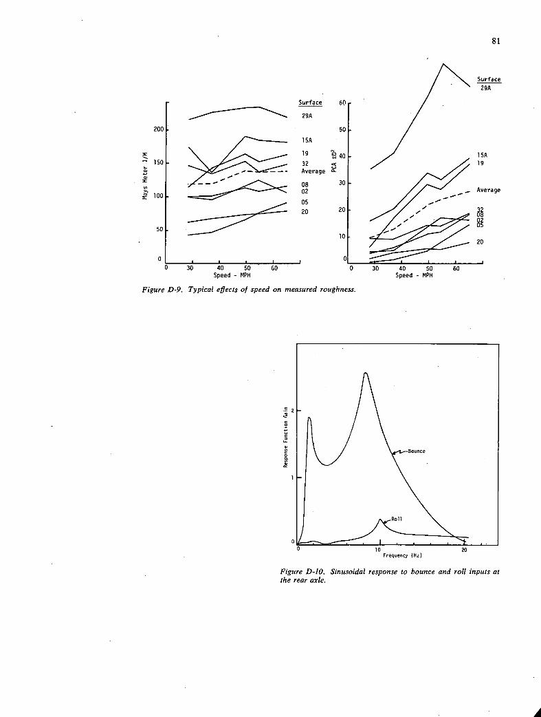
irf ace

9A

Surface

29A

200

- 150 S.- U U

>, 100

50

0

erage

15A

19 41 32

(-S Average -

08 31

02

05

20 21

81

'C

U 30 40 50 60 0 30 40 50

Speed - MPH Speed - MPH

Figure D-9. Typical effects of speed on measured roughness.

60

0 10 20 Frequency (Hz)

Figure D-10. Sinusoidal response to bounce and roll inputs at the rear axle.

THE TRANSPORTATION RESEARCH BOARD is an agency of the National Research. Council, which serves the National Academy of Sciences and the National Academy of Engineering. The Board's purpose is to stimulate research concerning the nature and performance of transportation systems, to disseminate information that the research produces, and to encourage the application of appropriate research findings. The Board's program is carried out by more than 250 committees, task forces, and panels composed of more than 3100 administrators, engineers, social scientists, attorneys, edu-cators, and others concerned with transportation; they serve without compensation. The program is supported by state transportation and highway departments, the modal ad-ministrations of the U.S. Department of Transportation, the Association of American Railroads, and other organizations and individuals interested in the development of transportation.

The Transportation Research Board operates within the Commission on Sociotechnical Systems of the National Research Council. The National Research Council was estab-lished by the National Academy of Sciences in 1916 to associate the broad community of science and technology with the Academy's purposes of furthering knowledge and of advising the Federal Government. The Council operates in accordance with general policies determined by the Academy under the authority of its congressional charter of 1863, which establishes the Academy as a private, nonprofit, self-governing membership corporation. The Council has become the principal operating agency of both the National Academy, of Sciences and the National Academy of Engineering in the con-duct of their services to the government, the public, and the scientific and engineering communities. It is administered jointly by both Academies and. the Institute of Medicine.

The National Academy of Sciences was established in 1863 by Act of Congress as a private, nonprofit, self-governing membership corporation for the furtherance of science and technology, required to advise the Federal. Government upon request within its fields of competence. Under its corporate charter the Academy established the National Research Council in 1916, the National, Academy of Engineering, in 1964,, and the. Institute of Medicine in 1970.

TRANSPORTATION RESEARCH BOARD National Research Council

2101 Constitution Avenue, N.W.

Washington, D.C. 20418

NON-PROFIT ORG.

U.S. POSTAGE

P A I D

WASHINGTON, D.C.

PERMIT NO. 42970 ADDRESS CORRECTION REQUESTED

0